Embed Size (px)
Citation preview
Benchmarking full-body inertial motion capture for clinical gait
analysis
Teunis Cloete
Final MSc Thesis Report
Department of Mechanical and Mechatronic Engineering
University of Stellenbosch
29 January 2009
- II -
Benchmarking full-body inertial motion capture for
clinical gait analysis
Final MSc Thesis Report
Teunis Cloete
Department of Mechanical and Mechatronic Engineering
Stellenbosch University
2nd
Edition
29 January 2009
Benchmarking full-body inertial motion capture for clinical gait analysis
Final MSc Thesis Report
Author: Mr. T. Cloete
Supervisor: Prof. C. Scheffer
Department of Mechanical and Mechatronic Engineering
University of Stellenbosch
2nd
Edition
29 January 2009
- I -
SUMMARY
Clinical gait analysis has been proven to greatly improve treatment planning and
monitoring of patients suffering from neuromuscular disorders. Despite this fact, it
was found that gait analysis is still largely underutilised in general patient-care due to
limitations of gait measurement equipment. Inertial motion capture (IMC) is able to
overcome many of these limitations, but this technology is relatively untested and is
therefore viewed as adolescent.
This study addresses this problem by evaluating the validity and repeatability of gait
parameters measured with a commercially available, full-body IMC system by
comparing the results to those obtained with alternative methods of motion capture.
The IMC system’s results were compared to a trusted optical motion capture (OMC)
system’s results to evaluate validity. The results show that the measurements for the
hip and knee obtained with IMC compares well with those obtained using OMC –
with coefficient-of-correlation (R) values as high as 0.99. Some discrepancies were
identified in the ankle-joint validity results. These were attributed to differences
between the two systems with regard to the definition of ankle joint and to non-ideal
IMC system foot-sensor design.
The repeatability, using the IMC system, was quantified using the coefficient of
variance (CV), the coefficient of multiple determination (CMD) and the coefficient of
multiple correlation (CMC). Results show that IMC-recorded gait patterns have high
repeatability for within-day tests (CMD: 0.786-0.984; CMC: 0.881-0.992) and
between-day tests (CMD: 0.771-0.991; CMC: 0.872-0.995). These results compare
well with those from similar studies done using OMC and electromagnetic motion
capture (EMC), especially when comparing between-day results.
Finally, to evaluate the measurements from the IMC system in a clinically useful
application, a neural network was employed to distinguish between gait strides of
stroke patients and those of able-bodied controls. The network proved to be very
successful with a repeatable accuracy of 99.4% (1/166 misclassified). The study
concluded that the full-body IMC system produces sufficiently valid and repeatable
gait data to be used in clinical gait analysis, but that further refinement of the ankle-
joint definition and improvements to the foot sensor are required.

- II -
OPSOMMING
Dit is bewys dat kliniese gang-analise tot groot verbeterings lei in die
versorgingsbeplanning en monitering van pasiënte wat aan neuromuskulêre siektes ly.
Ten spyte hiervan word daar gevind dat gang-analise steeds onderbenut word in
algemene pasiëntesorg vanweë tekortkominge in gang-opnametoerusting. Inersie-
bewegingsopname (IBO) bied oplossings vir vele van hierdie tekortkominge, maar
die tegnologie is steeds relatief ongetoets en word dus as onvolwasse beskou.
In hierdie studie word dié probleem aangespreek deur die geldigheid en
herhaalbaarheid van gang-parameters, wat met behulp van ’n kommersieel beskikbare
IBO-stelsel gemeet is, te ondersoek deur die resultate met alternatiewe
bewegingsopnamemetodes te vergelyk. Die IBO-stelsel is vergelyk met ’n betroubare
optiese bewegingsopname (OBO)-stelsel om die geldigheid te bepaal. Resultate toon
dat IBO-opnames goed vergelyk met dié van OBO wat geneem is van die heup en
knie met waardes van koëffisiënt van korrelasie (R) wat strek tot 0.99.
Geldigheidsresultate van die enkelgewrig toon swakker waardes. Die probleme word
toegeskryf aan verskille in die definisie van die enkelgewrig en die nie-ideale
ontwerp van die IBO-stelsel se voetsensor.
Die herhaalbaarheid van die IBO-resultate is gekwantifiseer met behulp van die
koëffisiënt van variasie (KV), koëffisiënt van veelvoudige determinasie (KVD) en die
koëffisiënt van veelvoudige korrelasie (KVK). Resultate het getoon dat gang-
opnames met behulp van die IBO-stelsel goeie herhaalbaarheid toon vir sowel
dieselfde-dag-toetse (KVD: 0.786-0.984; KVK: 0.881-0.992) en verskillende-dag-
toetse (KVD: 0.771-0.991 ; KVK: 0.872-0.995). Resultate vergelyk goed met dié van
soortgelyke studies wat gedoen is met behulp van OBO en elektromagnetiese
bewegingsopname (EBO), veral vir verskillende-dag resultate.
Om gang-opnames van die IBO-stelsel in ’n nuttige kliniese toepassing te ondersoek,
is ’n neurale netwerk ingespan om te onderskei tussen gang-opnames van pasiënte
met beroerte en gang-opnames van ’n kontrolegroep. Die netwerk het goeie resultate
getoon met ’n herhaalbare akkuraatheid van 99.4% (1/166 vals geklassifiseer). Die
gevolgtrekking van hierdie studie is dus dat die IBO-stelsel voldoende geldigheid en
herhaalbaarheid toon om van nut te wees vir kliniese gang-analise. Verdere verfyning
van die enkelgewrig-definisie en verbetering van die voetsensors is egter nodig.

- III -
ACKNOWLEDGEMENTS
To God goes all the Glory for without Him this project would not have been possible.
The author would like to give special thanks to Dr. Regan Arendse of the University
of Stellenbosch, Dept. of Medicine, for his help in the capture and processing of data
from the VICON optical motion capture system and to the University of Cape Town,
Dept. of Sport Science for the use of their VICON laboratory.
Thank you also to Mr Wasim Labban of the University of Stellenbosch, Dept. of
Physiotherapy, for his help with the recording and analysis of stroke patient data as
well as his help in the analysis of gait patterns.
Thank you also to the Biomedical Engineering Research Group at the University of
Stellenbosch, Dept. of Mechanical and Mechatronic Engineering, for their financial
support in this project.

- IV -
DECLARATION
I, the undersigned, hereby declare that the work contained in this thesis is my own
original work and that I have not previously in its entirety or in part submitted it at
any university for a degree.
Signature: ……………………………………………………
Teunis Cloete
Date: …………………………………………………………..
Copyright © 2008 Stellenbosch University.
All Rights reserved.
- V -
TABLE OF CONTENTS
Page
TABLE OF CONTENTS ................................................................................................................... V
NOMENCLATURE ........................................................................................................................ VII
LIST OF ABREVIATIONS ............................................................................................................ VII
LIST OF SYMBOLS ......................................................................................................................VIII
LIST OF UNITS .............................................................................................................................VIII
LIST OF FIGURES ........................................................................................................................... IX
LIST OF TABLES .............................................................................................................................. X
1. INTRODUCTION ..................................................................................................................... 1
1.1. INTRODUCTION ...................................................................................................................... 1 1.2. PROBLEM STATEMENT ........................................................................................................... 2 1.3. MOTIVATION ......................................................................................................................... 2 1.4. OBJECTIVES ........................................................................................................................... 3 1.5. SCOPE OF WORK .................................................................................................................... 4
2. LITERATURE REVIEW ......................................................................................................... 6
2.1. WHAT IS GAIT ANALYSIS? ..................................................................................................... 6 2.1.1. Pathological gait ........................................................................................................... 7 2.1.2. History of kinematic gait measurement ......................................................................... 8 2.1.3. Methods of quantifying human gait ............................................................................. 10
2.2. RELATED RESEARCH............................................................................................................ 19 2.2.1. Using motion capture for clinical gait analysis ........................................................... 19 2.2.2. Verification of inertial motion capture ........................................................................ 19 2.2.3. Repeatability in gait patterns ....................................................................................... 21
3. VALIDITY STUDY ................................................................................................................. 22
3.1. TEST PARTICIPATION ........................................................................................................... 22 3.1.1. Inclusion criteria ......................................................................................................... 22 3.1.2. Ethical approval / Protocol ......................................................................................... 22
3.2. APPARATUS ......................................................................................................................... 22 3.2.1. Vicon – Optical motion capture system ....................................................................... 22 3.2.2. Moven – Inertial motion capture system ...................................................................... 23
3.3. DATA ACQUISITION AND PROCESSING ................................................................................. 26 3.3.1. Test protocol ................................................................................................................ 26 3.3.2. File format ................................................................................................................... 29
3.4. DATA ANALYSIS .................................................................................................................. 30 3.4.1. Gait data representation .............................................................................................. 30 3.4.2. Graphical user interface .............................................................................................. 32 3.4.3. Synchronizing IMC and OMC data ............................................................................. 34 3.4.4. Statistical approach ..................................................................................................... 35
3.5. RESULTS .............................................................................................................................. 36 3.5.1. Temporal-spatial comparison ...................................................................................... 36 3.5.2. Joint angle comparison ............................................................................................... 36
3.6. DISCUSSION ......................................................................................................................... 42
- VI -
4. REPEATABILITY STUDY .................................................................................................... 45
4.1. TEST PARTICIPATION ........................................................................................................... 45 4.2. APPARATUS ......................................................................................................................... 45 4.3. DATA ACQUISITION AND PROCESSING ................................................................................. 45 4.4. DATA ANALYSIS .................................................................................................................. 46
4.4.1. Gait data representation .............................................................................................. 46 4.4.2. Statistical approach ..................................................................................................... 46
4.5. RESULTS .............................................................................................................................. 47 4.5.1. Temporal-spatial repeatability .................................................................................... 47 4.5.2. Joint angle repeatability .............................................................................................. 49
4.6. DISCUSSION ......................................................................................................................... 55
5. NEURAL NETWORK ............................................................................................................ 57
5.1. INTRODUCTION .................................................................................................................... 57 5.2. OBJECTIVES ......................................................................................................................... 57 5.3. PROCEDURE ......................................................................................................................... 57
5.3.1. Data collection ............................................................................................................ 57 5.3.2. Network input parameters ........................................................................................... 58 5.3.3. Training and testing the model .................................................................................... 62 5.3.4. Network training function selection ............................................................................. 62
5.4. RESULTS .............................................................................................................................. 64 5.5. DISCUSSION ......................................................................................................................... 66
6. CONCLUSION ........................................................................................................................ 68
6.1. USING FULL-BODY IMC IN EVERYDAY ACTIVITIES .............................................................. 68 6.2. TELEMEDICINE .................................................................................................................... 69 6.3. INERTIAL MOTION CAPTURE FOR CLINICAL GAIT ANALYSIS ................................................. 69 6.4. RECOMMENDATIONS ........................................................................................................... 70 6.5. FUTURE WORK ..................................................................................................................... 71
7. REFERENCES ........................................................................................................................ R1
8. APPENDICES ......................................................................................................................... A1
8.1. APPENDIX A: GAIT PARAMETERS ....................................................................................... A1 8.1.1. Temporal parameters .................................................................................................. A1 8.1.2. Spatial parameters ....................................................................................................... A2 8.1.3. Joint angles .................................................................................................................. A3
8.2. APPENDIX B: PATHOLOGICAL GAIT .................................................................................... A4 8.3. APPENDIX C: GAIT PARAMETER CALCULATION SCRIPT ...................................................... A5 8.4. APPENDIX D: VALIDITY STUDY RESULTS ........................................................................... A8
8.4.1. Temporal-spatial validity results ................................................................................. A8 8.4.2. Joint angle validity results ........................................................................................... A9 8.4.3. Joint angle validity results - Suit vs. straps ............................................................... A11
8.5. APPENDIX E: NEURAL NETWORK RESULTS ....................................................................... A12 8.5.1. TRAINLM .................................................................................................................. A12 8.5.2. TRAINGDM ............................................................................................................... A14 8.5.3. TRAINGDX ................................................................................................................ A16

- VII -
NOMENCLATURE
Normal gait Stride of an able-bodied human
Pathological gait Stride patterns showing locomotive irregularities
Orthopaedics A branch of surgery related to musculoskeletal injuries
Ambulation Movement related to walking (while walking)
Hemiparesis Loss of control of feeling in one half of the body
LIST OF ABREVIATIONS
IMC Inertial motion capture
OMC Optical motion capture
EMC Electromagnetic motion capture
MEM Microelectromechanical
GCS Global coordinate system
BCS Body coordinate system
JCS Joint coordinate system
AL Anatomical landform
ROM Range of motion
PD Parkinson’s disease
HS Heel-strike
TO Toe-off
DOF Degrees of freedom
R Correlation coefficient
CMD Coefficient of multiple determination
CMC Coefficient of multiple correlation
SD Standard deviation

- VIII -
LIST OF SYMBOLS
φ Roll
θ Elevation
ψ Azimuth
φh Hip abduction-adduction
θh Hip flexion-extension
ψh Hip internal-external rotation
φk Knee varus-valgus
θk Knee flexion-extension
ψk Knee internal-external rotation
φa Ankle eversion-inversion
θa Ankle plantar-dorsiflexion
ψa Ankle supination-pronation
M Total number of days (Section 4.4.2)
N Total number of runs (Section 4.4.2)
T Total stride-time (Section 4.4.2)
LIST OF UNITS
Hz Hertz
ms Milliseconds
g Gravitational acceleration
m/s Meters per second
kg Kilogram

- IX -
LIST OF FIGURES
Figure 1: Gait cycle ................................................................................................................... 6
Figure 2: Division of gait cycle ................................................................................................. 7
Figure 3: "The Human Figure in Motion" by Muybridge (1878) ............................................. 9
Figure 4: Braune and Fischer’s subject wearing the experimental suit ................................... 10
Figure 5: Mechanical motion capture devices......................................................................... 12
Figure 6: Electromagnetic motion capture system .................................................................. 13
Figure 7: Optical motion capture - Vicon Oxford Metrics Ltd. .............................................. 14
Figure 8: Markerless optical Mocap ....................................................................................... 15
Figure 9: Structure of Kalman filter estimation. ..................................................................... 16
Figure 10: Inertial motion sensors ........................................................................................... 16
Figure 11: Moven motion capture system ............................................................................... 23
Figure 12: Body segment coordinate system in global coordinate system ............................. 24
Figure 13: Marker and sensor placement ................................................................................ 27
Figure 14: OMC calibration procedures ................................................................................. 28
Figure 15: IMC calibration procedures ................................................................................... 28
Figure 16: Schematic of gait parameter calculation script ...................................................... 32
Figure 17: Graphical user interface ......................................................................................... 33
Figure 18: Heel-strike identification ....................................................................................... 35
Figure 19: Comparative data validity for the left side of a representative subject .................. 40
Figure 20: Comparative data validity for the right side of a representative subject ............... 42
Figure 21: Foot sensor position ............................................................................................... 44
Figure 22: Mean and standard deviation of temporal-spatial parameter repeatability for a
representative subject .............................................................................................................. 48
Figure 23: Mean and variance of joint angle motion of the right side for the representative
subject over nine runs ............................................................................................................. 53
Figure 24: Mean and variance of joint angle motion of the left side for the representative
subject over nine runs ............................................................................................................. 55
Figure 25: Scatter plots of neural network input variables ..................................................... 59
Figure 26: Temporal gait parameters ..................................................................................... A1
Figure 27: Spatial gait parameters .......................................................................................... A2
Figure 28: Schematic of gait parameter calculation script ..................................................... A5
- X -
LIST OF TABLES
Table 1: Summary of motion capture technologies ................................................................ 18
Table 2: Joint angles evaluated ............................................................................................... 31
Table 3: Temporal-spatial results - Normal walk .................................................................... 36
Table 4: Joint angle validity results - Normal walk (Straps) ................................................... 37
Table 5: Joint angle validity results - Normal walk (Suit) ...................................................... 37
Table 6: Difference between joint angle validity results of suit and straps - Normal walk .... 38
Table 7: Difference between joint angle validity results of suit and straps - Fast walk .......... 38
Table 8: Test subject characteristics (repeatability study) ...................................................... 45
Table 9: Comparison of intra-subject repeatability of temporal-spatial parameters ............... 48
Table 10: Within-day repeatability of joint angles – IMC vs. OMC ...................................... 49
Table 11: Within-day repeatability of joint angles – IMC vs. EMC ....................................... 49
Table 12: Between-day repeatability of joint angles – IMC vs. OMC.................................... 50
Table 13: Between-day repeatability of joint angles with mean of each day removed – IMC
vs. OMC .................................................................................................................................. 51
Table 14: Between-day repeatability of joint angles with mean of each day removed – IMC
vs. EMC .................................................................................................................................. 51
Table 15: Neural network input parameters ............................................................................ 60
Table 16: Average false instances of neural network results over 15 identical runs .............. 64
Table 17: Standard deviation of neural network results over 15 identical runs ...................... 64
Table 18: Average goal tolerance of neural network results over 15 identical runs ............... 65
Table 19: Standard deviation in goal tolerance of neural network results over 15 identical
runs .......................................................................................................................................... 65
Table 20: Selection of neural network input variable ............................................................. 66
Table 21: Temporal-spatial validity results - Slow walk (Suit) ............................................. A8
Table 22: Temporal-spatial validity results - Normal walk (Suit) ......................................... A8
Table 23: Temporal-spatial validity results - Slow walk (Straps) .......................................... A8
Table 24: Temporal-spatial validity results - Normal walk (Straps) ...................................... A8
Table 25: Slow walk joint angle validity results (Suit) .......................................................... A9
Table 26: Normal walk joint angle validity results (Suit) ...................................................... A9
Table 27: Fast walk joint angle validity results (Suit) ........................................................... A9
Table 28: Slow walk joint angle validity results (Straps) .................................................... A10
Table 29: Normal walk joint angle validity results (Straps) ................................................ A10
Table 30: Fast walk joint angle validity results (Straps) ...................................................... A10
- XI -
Table 31: Difference between joint angle validity results of suit and straps - Slow walk ... A11
Table 32: Difference between joint angle validity results of suit and straps - Normal walk A11
Table 33: Difference between joint angle validity results of suit and straps - Fast walk ..... A11
Table 34: Average false instances of neural network results over 15 identical runs ........... A12
Table 35: Standard deviation of neural network results over 15 identical runs ................... A12
Table 36: Average goal tolerance of neural network results over 15 identical runs ............ A13
Table 37: Standard deviation in goal tolerance of neural network results over 15 identical
runs ....................................................................................................................................... A13
Table 38: Average false instances of neural network results over 15 identical runs ........... A14
Table 39: Standard deviation of neural network results over 15 identical runs ................... A14
Table 40: Average goal tolerance of neural network results over 15 identical runs ............ A15
Table 41: Standard deviation in goal tolerance of neural network results over 15 identical
runs ....................................................................................................................................... A15
Table 42: Average false instances of neural network results over 15 identical runs ........... A16
Table 43: Standard deviation of neural network results over 15 identical runs ................... A16
Table 44: Average goal tolerance of neural network results over 15 identical runs ............ A17
Table 45: Standard deviation in goal tolerance of neural network results over 15 identical
runs ....................................................................................................................................... A17
BENCHMARKING FULL-BODY INERTIAL MOTION CAPTURE FOR CLINICAL GAIT ANALYSIS
TEUNIS CLOETE - 29 JANUARY 2009
DEPARTMENT OF MECHANICAL AND MECHATRONIC ENGINEERING - STELLENBOSCH UNIVERSITY
- 1 -
1. INTRODUCTION
1.1. Introduction
The analysis of human motion has progressed leaps and bounds from its origin in the
times of Aristotle and Borelli (Baker, 2007). Gait analysis is used to quantify the
mobility state of a person (Simon, 2004). This biomechanical information is useful in
several fields and applications, including: the ongoing pursuit for improved
performance and reduced injuries in athletes, the quest to make more believable
humanoid characters in computer graphics and virtual reality, the planning of
treatment protocols such as effective surgical intervention or orthopaedic prescription
(Roetenberg, 2006, Steinwender et al., 2000). Gait analysis also offers insight into the
development of motor learning skills in children, training development, rehabilitation
monitoring and the effect of neuromuscular injuries on a patient’s daily living
(Bronner, undated). The clinical applications mentioned are of greatest importance to
this study.
Current diagnostic observations of posture and movement made by physicians are
subjective and dependent on their judgment and experience (Lee et al., 2000, Mackey
et al., 2005). With the backing of several examples, Simon (2004) found that gait
analysis supplies a confidence not provided by regular clinical examination, that the
correct number and selection of surgical procedures can be chosen in patients with
cerebral palsy. This is also the case for patients with other neuromuscular disorders.
In spite of obvious advantages, gait analysis has nevertheless seen hampered
popularity and is still rarely used as a means of clinical diagnosis (Simon, 2004). The
limited utilization has been attributed to factors such as ineffective application of
current technologies and poor lab organization, test procedure, result interpretation
and report generation as well as the high cost associated with most gait studies. There
is often a need for gait analysis to be conducted outside of a laboratory environment
as in-lab walking differs from everyday walking (Simon, 2004). This attribute is also
a requirement in the field of telemedicine where doctors are unable to meet the
demand of patients in rural areas. Most gait labs are however unequipped to satisfy
this requirement.
In recent decades improvements in the field of photography have allowed researchers
to conduct frame-by-frame analyses of the mechanics of human motion. Ever-
increasing revelation of the clinical potential of gait analysis has united the medical
and engineering communities in efforts to fashion more efficient, accurate and
versatile ways of capturing and analysing human motion. Although originating from
clinical studies, the industry of motion capture (Mocap) has seen noticeable growth
with the more recent popularity of life-like computer animations in television and
computer gaming. This has birthed a variety of methods of Mocap, each with their
own advantages and limitations (as discussed in Section 2.1.3.2). The most common

BENCHMARKING FULL-BODY INERTIAL MOTION CAPTURE FOR CLINICAL GAIT ANALYSIS
TEUNIS CLOETE - 29 JANUARY 2009
DEPARTMENT OF MECHANICAL AND MECHATRONIC ENGINEERING - STELLENBOSCH UNIVERSITY
- 2 -
limitation in Mocap systems is their high cost and spatial restrictions. In almost all
cases Mocap is conducted indoors and within limited spatial boundaries (Vlasic et al.,
2007). Only recently has technology allowed for the development of untethered
Mocap such as magnetic and inertial motion capture (IMC). This is largely because of
recent advances in Micro Electro Mechanical System (MEMS) technologies
encouraging the development of small and inexpensive sensors such as
accelerometers, gyroscopes and magnetometers which form the key components of
inertial motion sensor units. These sensors allow researchers to determine orientation
based on passive measurements of physical quantities directly related to the motion
and orientation of rigid bodies to which the sensors are attached (Bachmann, 2000).
These, along with powerful microcontrollers, small batteries and high storage
capacities directly facilitate long term, portable recordings of ambulatory
measurements (Dejnabadi et al., 2005).
With evident versatility and cost advantages over alternative, laboratory-based
optical, acoustic and mechanical systems, it would seem that IMC offers solutions to
several of the before-mentioned hampering factors. It is thus applicable to ask why
IMC is still largely underutilized for clinical gait analysis. A possible answer lies in
the adolescence of the technology in practice, and therefore the lack of confidence in
its measurement accuracy. This study aims to address this hindrance by investigating
the validity and repeatability of results obtained from a commercially available, full-
body IMC system, by comparing them to results obtained from a proven and
commonly used optical motion capture (OMC) system. Various studies have been
conducted to compare these technologies (Dejnabadi et al., 2005, Dejnabadi et al.,
2006, Favre et al., 2006, Roetenberg, 2006, Simon, 2004), however the author has
found no evidence of such a comparison done during a routine ambulatory gait
analysis.
1.2. Problem statement
Mocap methods currently used for clinical gait analysis are sufficiently accurate and
well accepted among professionals in the field. However, these Mocap systems often
lack spatial versatility and are relatively costly. Cheaper, more flexible methods of
recording motion have emerged in recent years, but these are relatively untested in
relevant applications and therefore invoke uncertainties among physicians.
1.3. Motivation
As mentioned above, there are several factors which limit the widespread utilization
of gait analysis as an everyday clinical tool. These are summarized below:
i. Gait analysis is primarily considered by most physicians to be a research
tool rather than an aid to clinical decision-making. This view is often

BENCHMARKING FULL-BODY INERTIAL MOTION CAPTURE FOR CLINICAL GAIT ANALYSIS
TEUNIS CLOETE - 29 JANUARY 2009
DEPARTMENT OF MECHANICAL AND MECHATRONIC ENGINEERING - STELLENBOSCH UNIVERSITY
- 3 -
supported by the fact that medical insurance companies do not cover gait
analysis in their policies (Simon, 2004).
ii. Gait laboratories are viewed as inefficient, unproductive and
uneconomical because:
o The laboratory setup and calibration procedures vary from test-to-test
and patient-to-patient, making the procedure time consuming and
therefore limiting the daily patient throughput.
o In most cases trained professionals are employed to acquire process
and interpret gait data. Associated labour costs are considered as the
major contributor to the relatively high cost of gait tests.
o Gait test reports, generated for physicians, are often tardy and contain
vast amounts of unnecessary data (Simon, 2004).
iii. Gait parameters are calculated using assumptions of skin movement and
anatomical parameters to estimate joint angle centres rather than actual
measured data (Simon, 2004). According to White et al. (1989) there are
inherent errors associated with anatomical variability in bony contours and
muscle attachment (White et al., 1989). This forces physicians to question
the validity of measured gait parameters.
iv. Most gait analyses are conducted within laboratories which limits both the
range of motion and duration of tests. In several applications, including
rehabilitation and sports performance analysis, it may be necessary that
gait recordings be done in larger and more versatile locations. Long term
gait assessments are often required for patients with neuromuscular
disorders and ideally in the patient’s everyday home environments (refer
to Section 2.1.1).
v. Economic as well as logistical reasons cause trained physicians to be
predominantly based in urban areas. This relates to hampered health care
(such as gait analysis) for patients restricted to rural areas.
vi. Current methods of recording the 3D kinematics suffer from several
problems which cause uncertainty about their validity. According to
Bachmann (2000) these include: Marginal accuracy, user encumbrance,
range restrictions, susceptibility to interference, noise, poor registration,
occlusion difficulties and high latency. These limitations in Mocap
technologies are further discussed in Section 2.1.3.2
1.4. Objectives
In order to address the listed factors which have curbed gait analysis from becoming a
commonly used diagnostic tool, the following objectives can be suggested:

BENCHMARKING FULL-BODY INERTIAL MOTION CAPTURE FOR CLINICAL GAIT ANALYSIS
TEUNIS CLOETE - 29 JANUARY 2009
DEPARTMENT OF MECHANICAL AND MECHATRONIC ENGINEERING - STELLENBOSCH UNIVERSITY
- 4 -
i. To identify the most significant limitations to current means of conducting
3D kinematic gait analysis.
ii. To identify and define the requirements of a full-body motion capture
system necessary for accurate and reliable gait analysis.
iii. To both qualitatively and quantitatively test whether IMC offers a solution
to the above-mentioned limitations.
iv. To test the use of IMC in a clinical application through implementing a
neural network, using IMC collected gait data, to distinguish between able-
bodied subjects and stroke patients.
v. To discuss the aptness of IMC as a telemedicine tool.
vi. To suggest possible improvements to current methods of Mocap and
subsequent gait data acquisition and analysis.
1.5. Scope of work
This study consists of four major sections, namely: 1) A literature review in which
the current state of the art in motion capture methods are compared to the current
requirements of clinical gait analysis. 2) A validity study in which inertial motion
capture is compared to a generally accepted “gold standard” Mocap system on the
grounds of statistical accuracy and precision. 3) A repeatability study in which the
within-day and between test day repeatability is evaluated for both able-bodied and
gait impaired ambulators. 4) The application of a neural network to test IMC
collected gait data in a clinical application. This thesis represents the study findings
and is organized as follows:
Chapter 2 defines and describes gait analysis and its historical background and
continues with a look at its application in the diagnosis, assessment and treatment of
patients with pathological (abnormal) gait. In Section 2.1.3.2, a qualitative
comparison is drawn between the advantages and shortcomings of the most popular
methods of Mocap. This includes an investigation into the ways in which gait
parameters are acquired, calculated and represented. Finally, Section 2.2 contains a
discussion of the procedures and findings of other studies related to this one.
Chapter 3 and 4 include the objectives, procedure, statistical approach and post-
processing of the validity and repeatability studies respectively, as well as discussions
on their findings with reference to related literature.
Chapter 5 discusses the planning, implementation, analysis and results of the neural
network.

BENCHMARKING FULL-BODY INERTIAL MOTION CAPTURE FOR CLINICAL GAIT ANALYSIS
TEUNIS CLOETE - 29 JANUARY 2009
DEPARTMENT OF MECHANICAL AND MECHATRONIC ENGINEERING - STELLENBOSCH UNIVERSITY
- 5 -
Chapter 6 examines IMC in everyday activities and considers its usefulness in
telemedicine. The chapter then concludes the thesis by holistically discussing the
results with reference to the objectives listed in Section 1.4 and, with these in mind,
provides recommendations for future studies.
BENCHMARKING FULL-BODY INERTIAL MOTION CAPTURE FOR CLINICAL GAIT ANALYSIS
TEUNIS CLOETE - 29 JANUARY 2009
DEPARTMENT OF MECHANICAL AND MECHATRONIC ENGINEERING - STELLENBOSCH UNIVERSITY
- 6 -
2. LITERATURE REVIEW
2.1. What is gait analysis?
Ambulation in humans can be defined as upright, bipedal locomotion, or gait
(Whiting and Rugg, 2006). According to Whiting and Rugg (2006), gait analysis is
the study of a particular form of human or animal1 locomotion. Gait is typically used
to describe a walking or running movement. Han, et al. (2006) describes gait as a
cyclic movement of the feet in which one or the other alternate in contact with the
ground. Gait analysis forms part of the field of biomechanics which includes statics
and dynamics, the latter comprising of kinetic and kinematic parameter (Bronner,
undated). Kinematic parameters may be further sub-divided into temporal-spatial and
3D joint angles. A human stride can be quantified by what is commonly referred to as
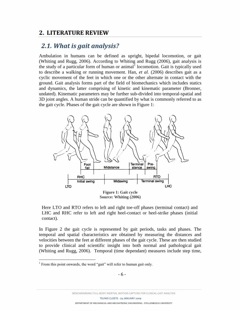
the gait cycle. Phases of the gait cycle are shown in Figure 1:
Figure 1: Gait cycle
Source: Whiting (2006)
Here LTO and RTO refers to left and right toe-off phases (terminal contact) and
LHC and RHC refer to left and right heel-contact or heel-strike phases (initial
contact).
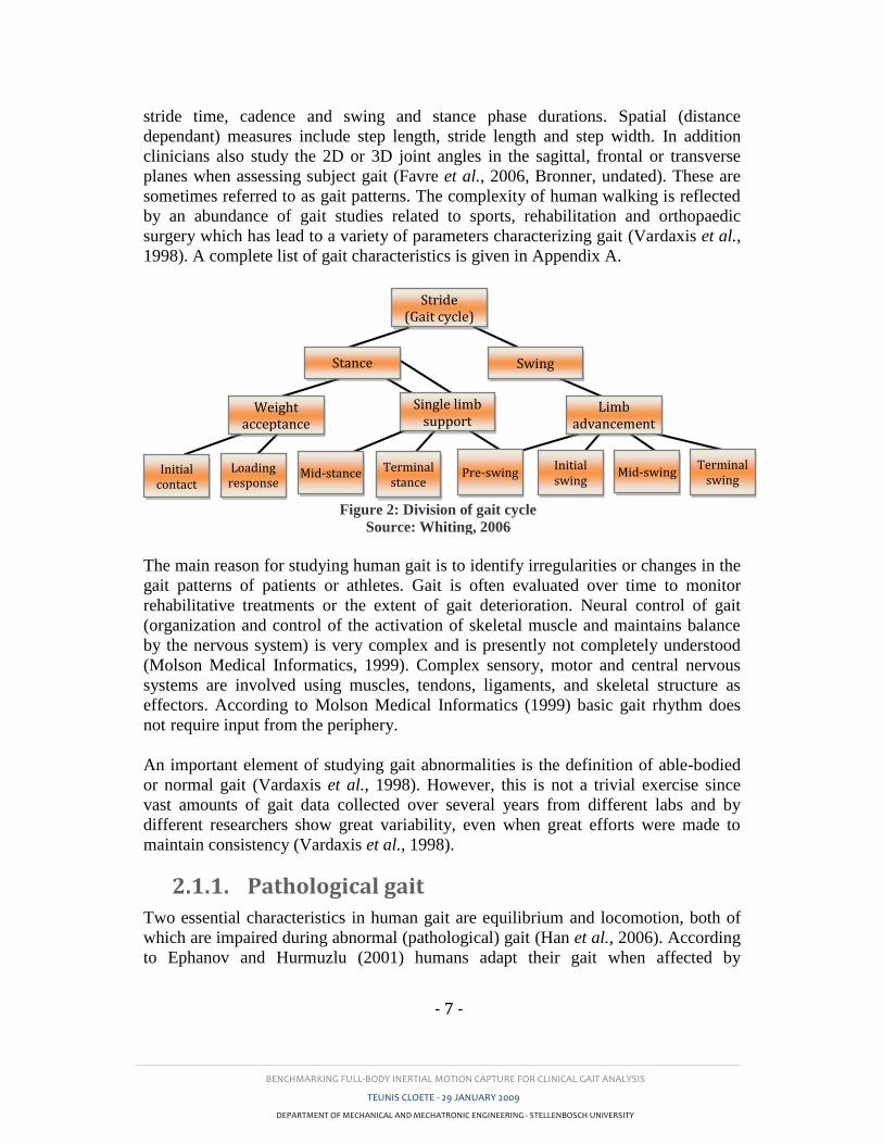
In Figure 2 the gait cycle is represented by gait periods, tasks and phases. The
temporal and spatial characteristics are obtained by measuring the distances and
velocities between the feet at different phases of the gait cycle. These are then studied
to provide clinical and scientific insight into both normal and pathological gait
(Whiting and Rugg, 2006). Temporal (time dependant) measures include step time,
1 From this point onwards, the word “gait” will refer to human gait only.
BENCHMARKING FULL-BODY INERTIAL MOTION CAPTURE FOR CLINICAL GAIT ANALYSIS
TEUNIS CLOETE - 29 JANUARY 2009
DEPARTMENT OF MECHANICAL AND MECHATRONIC ENGINEERING - STELLENBOSCH UNIVERSITY
- 7 -
stride time, cadence and swing and stance phase durations. Spatial (distance
dependant) measures include step length, stride length and step width. In addition
clinicians also study the 2D or 3D joint angles in the sagittal, frontal or transverse
planes when assessing subject gait (Favre et al., 2006, Bronner, undated). These are
sometimes referred to as gait patterns. The complexity of human walking is reflected
by an abundance of gait studies related to sports, rehabilitation and orthopaedic
surgery which has lead to a variety of parameters characterizing gait (Vardaxis et al.,
1998). A complete list of gait characteristics is given in Appendix A.
The main reason for studying human gait is to identify irregularities or changes in the
gait patterns of patients or athletes. Gait is often evaluated over time to monitor
rehabilitative treatments or the extent of gait deterioration. Neural control of gait
(organization and control of the activation of skeletal muscle and maintains balance
by the nervous system) is very complex and is presently not completely understood
(Molson Medical Informatics, 1999). Complex sensory, motor and central nervous
systems are involved using muscles, tendons, ligaments, and skeletal structure as
effectors. According to Molson Medical Informatics (1999) basic gait rhythm does
not require input from the periphery.
An important element of studying gait abnormalities is the definition of able-bodied
or normal gait (Vardaxis et al., 1998). However, this is not a trivial exercise since
vast amounts of gait data collected over several years from different labs and by
different researchers show great variability, even when great efforts were made to
maintain consistency (Vardaxis et al., 1998).
2.1.1. Pathological gait
Two essential characteristics in human gait are equilibrium and locomotion, both of
which are impaired during abnormal (pathological) gait (Han et al., 2006). According
to Ephanov and Hurmuzlu (2001) humans adapt their gait when affected by
Figure 2: Division of gait cycle
Source: Whiting, 2006
Stride (Gait cycle)
Single limb support
Initial swing
Mid-swing Terminal
swing
Limb advancement
Swing Stance
Weight acceptance
Initial contact
Loading response
Mid-stance Terminal stance
Pre-swing
BENCHMARKING FULL-BODY INERTIAL MOTION CAPTURE FOR CLINICAL GAIT ANALYSIS
TEUNIS CLOETE - 29 JANUARY 2009
DEPARTMENT OF MECHANICAL AND MECHATRONIC ENGINEERING - STELLENBOSCH UNIVERSITY
- 8 -
pathological conditions to preserve their locomotive functionality. This is usually on
a subconscious level. Adaptive mechanisms such as reduced stride length and gait
cycle period are used by patients to reduce pain caused by joint moments (Gök et al.,
2002). This is exhibited by patients with Parkinson’s disease (PD) who tend to walk
slowly with short shuffling steps, reduced arm swing, stooped posture (Salarian et al.,
2004).
Stroke is a localized loss of brain function caused by a sudden lack of blood supply to
an area in the brain. Stroke may occur as a result of an embolism or haemorrhage.
Hemiparetic-stroke ambulation is characterised by asymmetry of temporal-spatial
parameters and joint angles between the paretic and non-paretic sides. One example
may be a lower hip extension measured on the paretic side compared to the
unaffected side. Other factors such as muscle or tendon infection, disease, paralysis,
injury and anatomical defects may also lead to abnormal gait. Gait disorders with
varying severity and blatancy have been extensively studied, but despite this, gait
analysis is rarely used to diagnose gait disorders (Simon, 2004). A list of structural
and neurological gait disturbances is given in Appendix B.
In recent years healthcare systems have promoted the idea of patient monitoring in
their own home environments (Roetenberg, 2006). This is particularly advantageous
when monitoring patients with Parkinson’s disease whose gait measurements are
significantly affected by the amount of medication in their bodies at the time (Han et
al., 2006). Several studies have emerged focusing on portable, comfortable and user-
friendly monitoring systems for stroke patients and patients suffering from
Parkinson’s disease and cerebral palsy (von Acht et al., 2007, Zhou and Hu, 2004,
Aminian et al., 2001, Han et al., 2006, Salarian et al., 2004). These, along with
statistical diagnostic algorithms could see future patient monitoring become both
simple and affordable. Simon (2004) suggested the use of advanced semi-automated-
diagnosis tools such as neural networks to assist in making gait analysis a part of a
physician’s referral process. With this in mind the focus must turn to optimizing
current methods of gait measurement and analysis.
2.1.2. History of kinematic gait measurement
The earliest recorded comments of human walking characteristics can be dated back
to Aristotle, who lived 384-322 BC. He stated that:
“If a man were to walk on the ground alongside a wall with a reed dipped in ink
attached to his head the line traced by the reed would not be straight but zig-zag,
because it goes lower when he bends and higher when he stands upright and raises
himself” (Baker, 2007).
Further progress only continued with experiments by Giovanni Borelli (1608–1679).
Several scientists wrote about walking through the enlightenment period, but it was
BENCHMARKING FULL-BODY INERTIAL MOTION CAPTURE FOR CLINICAL GAIT ANALYSIS
TEUNIS CLOETE - 29 JANUARY 2009
DEPARTMENT OF MECHANICAL AND MECHATRONIC ENGINEERING - STELLENBOSCH UNIVERSITY
- 9 -
the brothers Willhelm (1804–1891) and Eduard (1806–1871) Weber who made the
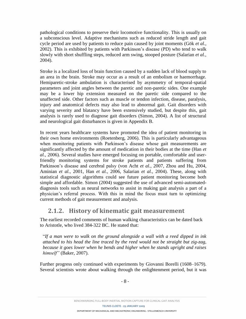
next significant contribution based on very simple measurements. Advancements in
gait measuring technologies were made in the early 1900s by Eadweard Muybridge in
California and Étienne-Jules Marey in Paris using still cameras. Refer to Figure 3
below.
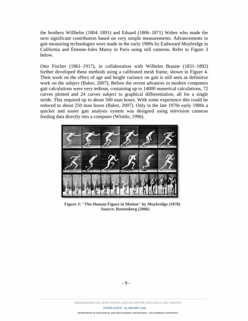
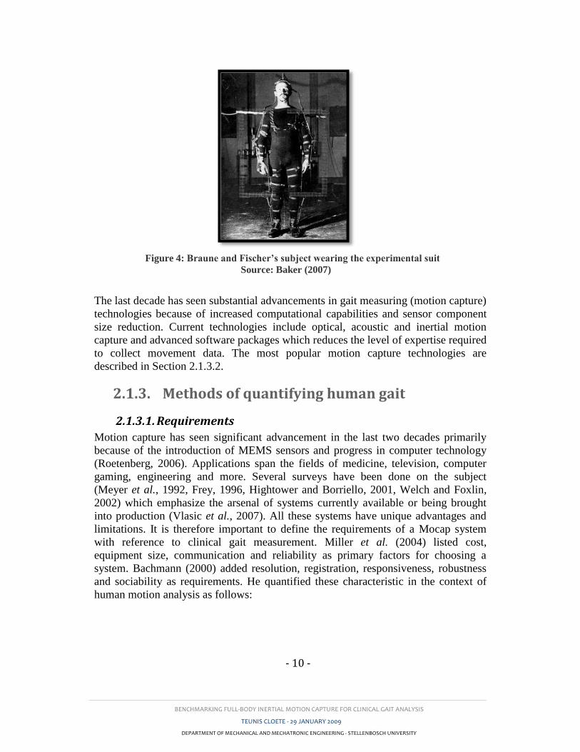
Otto Fischer (1861–1917), in collaboration with Wilhelm Braune (1831–1892)
further developed these methods using a calibrated mesh frame, shown in Figure 4.
Their work on the effect of age and height variance on gait is still seen as definitive
work on the subject (Baker, 2007). Before the recent advances in modern computers
gait calculations were very tedious, containing up to 14000 numerical calculations, 72
curves plotted and 24 curves subject to graphical differentiation, all for a single
stride. This required up to about 500 man hours. With some experience this could be
reduced to about 250 man hours (Baker, 2007). Only in the late 1970s early 1980s a
quicker and easier gait analysis system was designed using television cameras
feeding data directly into a computer (Whittle, 1996).
Figure 3: "The Human Figure in Motion" by Muybridge (1878)
Source: Roetenberg (2006)
BENCHMARKING FULL-BODY INERTIAL MOTION CAPTURE FOR CLINICAL GAIT ANALYSIS
TEUNIS CLOETE - 29 JANUARY 2009
DEPARTMENT OF MECHANICAL AND MECHATRONIC ENGINEERING - STELLENBOSCH UNIVERSITY
- 10 -
Figure 4: Braune and Fischer’s subject wearing the experimental suit
Source: Baker (2007)
The last decade has seen substantial advancements in gait measuring (motion capture)
technologies because of increased computational capabilities and sensor component
size reduction. Current technologies include optical, acoustic and inertial motion
capture and advanced software packages which reduces the level of expertise required
to collect movement data. The most popular motion capture technologies are
described in Section 2.1.3.2.
2.1.3. Methods of quantifying human gait
2.1.3.1. Requirements
Motion capture has seen significant advancement in the last two decades primarily
because of the introduction of MEMS sensors and progress in computer technology
(Roetenberg, 2006). Applications span the fields of medicine, television, computer
gaming, engineering and more. Several surveys have been done on the subject
(Meyer et al., 1992, Frey, 1996, Hightower and Borriello, 2001, Welch and Foxlin,
2002) which emphasize the arsenal of systems currently available or being brought
into production (Vlasic et al., 2007). All these systems have unique advantages and
limitations. It is therefore important to define the requirements of a Mocap system
with reference to clinical gait measurement. Miller et al. (2004) listed cost,
equipment size, communication and reliability as primary factors for choosing a
system. Bachmann (2000) added resolution, registration, responsiveness, robustness
and sociability as requirements. He quantified these characteristic in the context of
human motion analysis as follows:
BENCHMARKING FULL-BODY INERTIAL MOTION CAPTURE FOR CLINICAL GAIT ANALYSIS
TEUNIS CLOETE - 29 JANUARY 2009
DEPARTMENT OF MECHANICAL AND MECHATRONIC ENGINEERING - STELLENBOSCH UNIVERSITY
- 11 -
o The hand is viewed as the part of the body that experiences the greatest
motion and therefore governs the speed, force, frequency and precision
requirements.
o Fast hand motions occur at an average frequency of approximately 5 Hz.
Based on the Nyquist sampling theorem a 10 Hz sampling frequency should
be sufficient. However with the addition of noise from low cost sensors, and
thus applying a low pass filter and a rule of thumb of 20 times over-sampling,
the required sampling frequency is 100 Hz.
o Under normal circumstances the hand reaches a velocity of 3 m/s, but under
extreme conditions (such as throwing a baseball) it can reach up to 37 m/s.
o Normal hand movements generate accelerations of between 5 and 6 g, but
this may reach up to 25 g.
o The minimum changes in rotation angles perceivable to humans are
approximately 2.5°, 2° and 0.8° for the fingers, wrist and shoulders
respectively. An angular precision of 0.5° should therefore suffice.
o In applications where real-time movements are required (such as for patient
feedback) it was found that a lag of greater than 100 ms will degrade response
performance.
Sociability refers to the ability of the Mocap system to be used with other applicable
equipment. This could include physiological measurement devices such as EMG
force plates, or it may refer to equipment, such as a treadmill, sometimes necessary to
fully analyse a person’s gait. Frey et al. (1996) stated that a minimum of 15 body
segments have to be tracked to achieve full-body tracking. Untracked segments may
be added, but the kinematics of these would have to be calculated using reverse
kinematics which is computationally demanding (Frey et al., 1996).
2.1.3.2. Motion capture technologies
Some of the most popular Mocap technologies along with their relevant advantages
and limitations are described below:
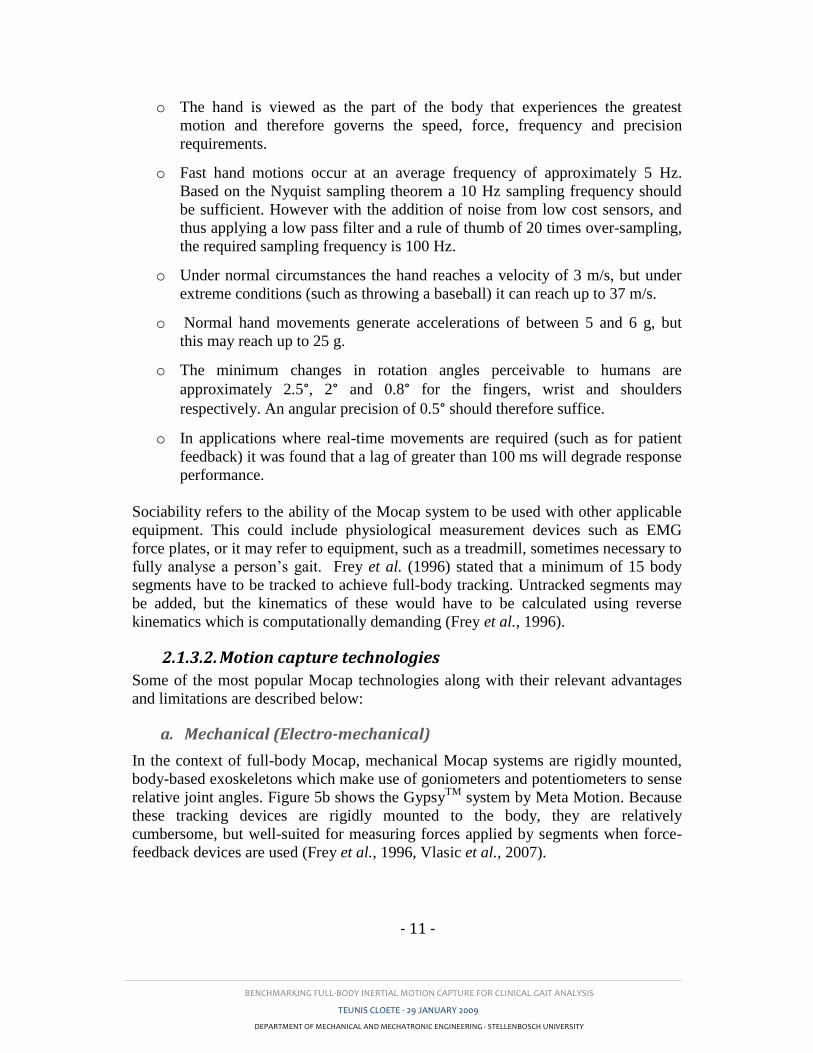
a. Mechanical (Electro-mechanical)
In the context of full-body Mocap, mechanical Mocap systems are rigidly mounted,
body-based exoskeletons which make use of goniometers and potentiometers to sense
relative joint angles. Figure 5b shows the GypsyTM
system by Meta Motion. Because
these tracking devices are rigidly mounted to the body, they are relatively
cumbersome, but well-suited for measuring forces applied by segments when force-
feedback devices are used (Frey et al., 1996, Vlasic et al., 2007).
BENCHMARKING FULL-BODY INERTIAL MOTION CAPTURE FOR CLINICAL GAIT ANALYSIS
TEUNIS CLOETE - 29 JANUARY 2009
DEPARTMENT OF MECHANICAL AND MECHATRONIC ENGINEERING - STELLENBOSCH UNIVERSITY
- 12 -
These systems are low in cost, and because no trigonometric calculations are
required, they are able to track the body segment orientation in real time (Bronner,
undated). These systems do not suffer from shadowing or interference problems
associated with other methods. On the downside, mechanical Mocap systems are
sensitive to soft-tissue artefacts and need a supplementary system to determine
segment position in a global coordinate system (GCS) (Roetenberg et al., 2007,
Bronner, undated).
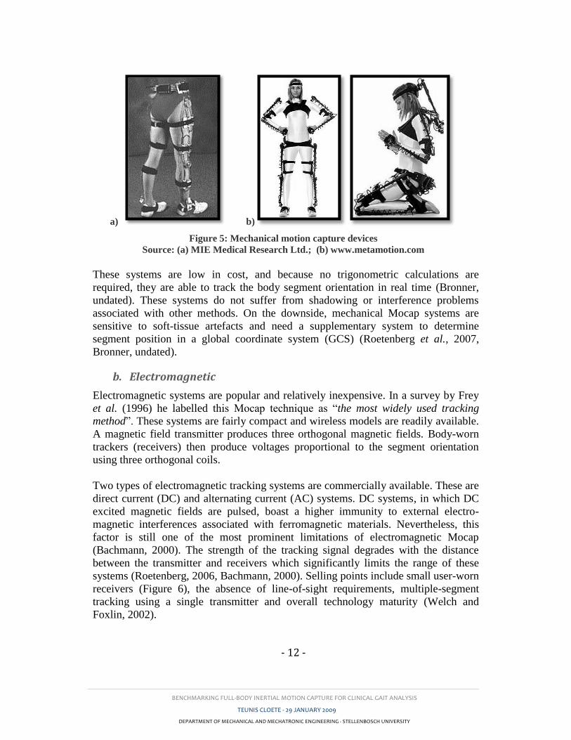
b. Electromagnetic
Electromagnetic systems are popular and relatively inexpensive. In a survey by Frey
et al. (1996) he labelled this Mocap technique as “the most widely used tracking
method”. These systems are fairly compact and wireless models are readily available.
A magnetic field transmitter produces three orthogonal magnetic fields. Body-worn
trackers (receivers) then produce voltages proportional to the segment orientation
using three orthogonal coils.
Two types of electromagnetic tracking systems are commercially available. These are
direct current (DC) and alternating current (AC) systems. DC systems, in which DC
excited magnetic fields are pulsed, boast a higher immunity to external electro-
magnetic interferences associated with ferromagnetic materials. Nevertheless, this
factor is still one of the most prominent limitations of electromagnetic Mocap
(Bachmann, 2000). The strength of the tracking signal degrades with the distance
between the transmitter and receivers which significantly limits the range of these
systems (Roetenberg, 2006, Bachmann, 2000). Selling points include small user-worn
receivers (Figure 6), the absence of line-of-sight requirements, multiple-segment
tracking using a single transmitter and overall technology maturity (Welch and
Foxlin, 2002).
a) b)
Figure 5: Mechanical motion capture devices
Source: (a) MIE Medical Research Ltd.; (b) www.metamotion.com
BENCHMARKING FULL-BODY INERTIAL MOTION CAPTURE FOR CLINICAL GAIT ANALYSIS
TEUNIS CLOETE - 29 JANUARY 2009
DEPARTMENT OF MECHANICAL AND MECHATRONIC ENGINEERING - STELLENBOSCH UNIVERSITY
- 13 -
a) b) Figure 6: Electromagnetic motion capture system
Source: Ascension Technology Corporation (2007)
c. Acoustic
Two methods of acoustic tracking are commonly in practice. The first employs the
time-of-flight (TOF) of sound waves where the body or segment is tracked by
measuring the distance between an acoustic pulse transmitter and a receiver at
different intervals in time. The speed of sonic or ultrasonic sound waves is used to
compute relative distances. Triangulation is used to track a relative position of a
segment. Where the position of more than one segment needs to be tracked
simultaneously, either a separate transmitter and receiver are required for every
segment or multiple frequency acoustics are used. To track the orientation of a
segment, two tracked points are required for each segment.
The second acoustic tracking technique uses the phase difference between incident
and returning sound waves to determine the position and orientation of the segment.
This technique is more accurate than TOF tracking, but is limited to calculating only
relative positions between points in contrast to full 3D position in the GCS which
TOF tracking is able to do (Frey et al., 1996), (Welch and Foxlin, 2002).
Acoustic tracking demonstrate superior range to electromagnetic tracking, but
requires a line-of-sight between emitters and receivers. Interference from echoing and
environmental noise deteriorates measurement quality.
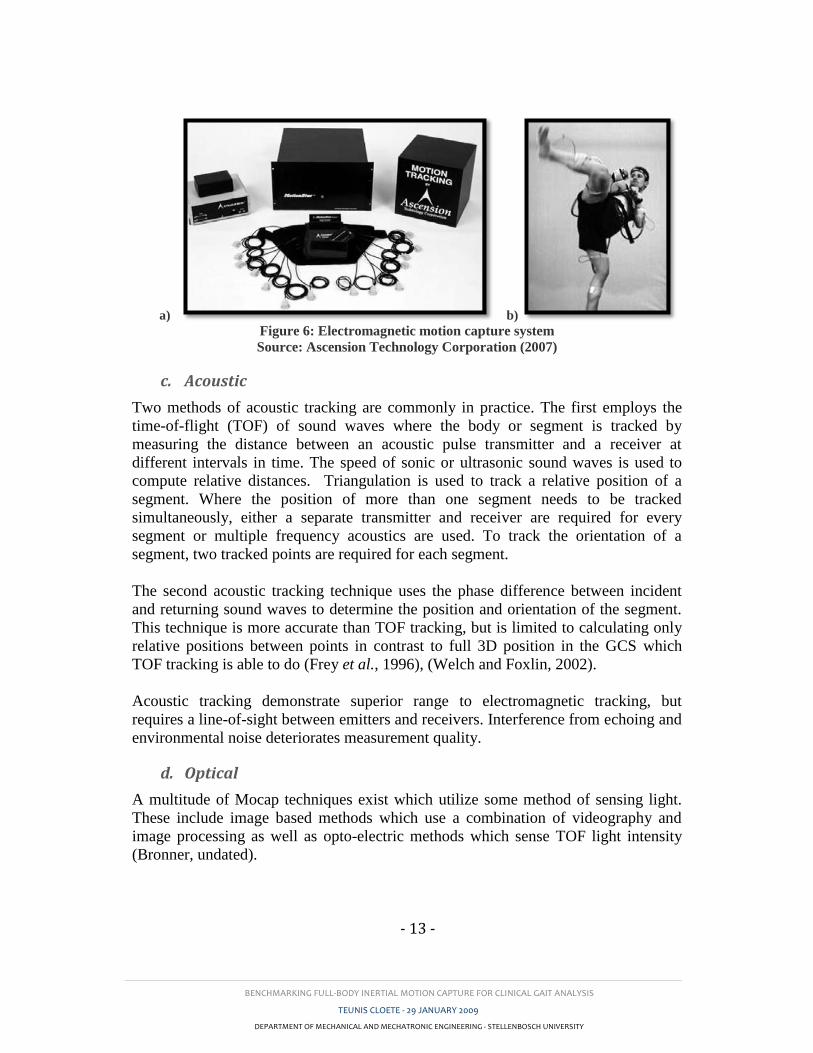
d. Optical
A multitude of Mocap techniques exist which utilize some method of sensing light.
These include image based methods which use a combination of videography and
image processing as well as opto-electric methods which sense TOF light intensity
(Bronner, undated).
BENCHMARKING FULL-BODY INERTIAL MOTION CAPTURE FOR CLINICAL GAIT ANALYSIS
TEUNIS CLOETE - 29 JANUARY 2009
DEPARTMENT OF MECHANICAL AND MECHATRONIC ENGINEERING - STELLENBOSCH UNIVERSITY
- 14 -
a) b)
Figure 7: Optical motion capture - Vicon Oxford Metrics Ltd.
Source: (a) www.bbc.co.uk; (b) www.rehabtrials.org
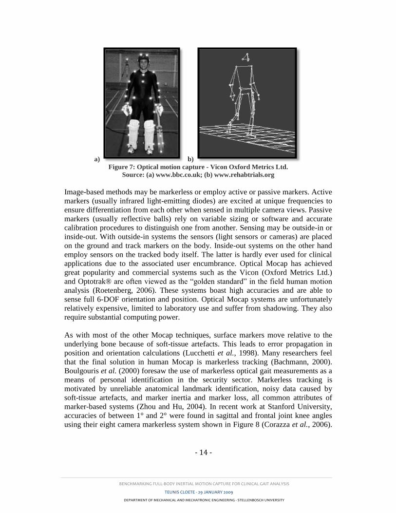
Image-based methods may be markerless or employ active or passive markers. Active
markers (usually infrared light-emitting diodes) are excited at unique frequencies to
ensure differentiation from each other when sensed in multiple camera views. Passive
markers (usually reflective balls) rely on variable sizing or software and accurate
calibration procedures to distinguish one from another. Sensing may be outside-in or
inside-out. With outside-in systems the sensors (light sensors or cameras) are placed
on the ground and track markers on the body. Inside-out systems on the other hand
employ sensors on the tracked body itself. The latter is hardly ever used for clinical
applications due to the associated user encumbrance. Optical Mocap has achieved
great popularity and commercial systems such as the Vicon (Oxford Metrics Ltd.)
and Optotrak® are often viewed as the “golden standard” in the field human motion
analysis (Roetenberg, 2006). These systems boast high accuracies and are able to
sense full 6-DOF orientation and position. Optical Mocap systems are unfortunately
relatively expensive, limited to laboratory use and suffer from shadowing. They also
require substantial computing power.
As with most of the other Mocap techniques, surface markers move relative to the
underlying bone because of soft-tissue artefacts. This leads to error propagation in
position and orientation calculations (Lucchetti et al., 1998). Many researchers feel
that the final solution in human Mocap is markerless tracking (Bachmann, 2000).
Boulgouris et al. (2000) foresaw the use of markerless optical gait measurements as a
means of personal identification in the security sector. Markerless tracking is
motivated by unreliable anatomical landmark identification, noisy data caused by
soft-tissue artefacts, and marker inertia and marker loss, all common attributes of
marker-based systems (Zhou and Hu, 2004). In recent work at Stanford University,
accuracies of between 1° and 2° were found in sagittal and frontal joint knee angles
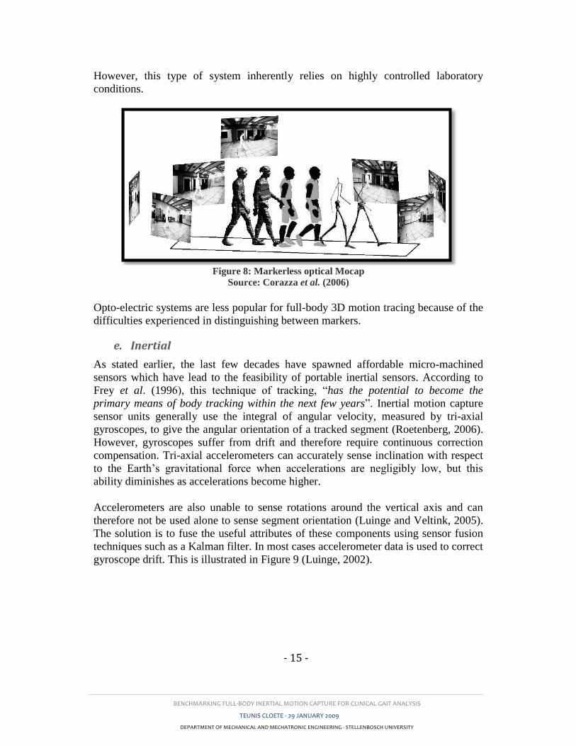
using their eight camera markerless system shown in Figure 8 (Corazza et al., 2006).
BENCHMARKING FULL-BODY INERTIAL MOTION CAPTURE FOR CLINICAL GAIT ANALYSIS
TEUNIS CLOETE - 29 JANUARY 2009
DEPARTMENT OF MECHANICAL AND MECHATRONIC ENGINEERING - STELLENBOSCH UNIVERSITY
- 15 -
However, this type of system inherently relies on highly controlled laboratory
conditions.
Figure 8: Markerless optical Mocap
Source: Corazza et al. (2006)
Opto-electric systems are less popular for full-body 3D motion tracing because of the
difficulties experienced in distinguishing between markers.
e. Inertial
As stated earlier, the last few decades have spawned affordable micro-machined
sensors which have lead to the feasibility of portable inertial sensors. According to
Frey et al. (1996), this technique of tracking, “has the potential to become the
primary means of body tracking within the next few years”. Inertial motion capture
sensor units generally use the integral of angular velocity, measured by tri-axial
gyroscopes, to give the angular orientation of a tracked segment (Roetenberg, 2006).
However, gyroscopes suffer from drift and therefore require continuous correction
compensation. Tri-axial accelerometers can accurately sense inclination with respect
to the Earth’s gravitational force when accelerations are negligibly low, but this
ability diminishes as accelerations become higher.
Accelerometers are also unable to sense rotations around the vertical axis and can
therefore not be used alone to sense segment orientation (Luinge and Veltink, 2005).
The solution is to fuse the useful attributes of these components using sensor fusion
techniques such as a Kalman filter. In most cases accelerometer data is used to correct
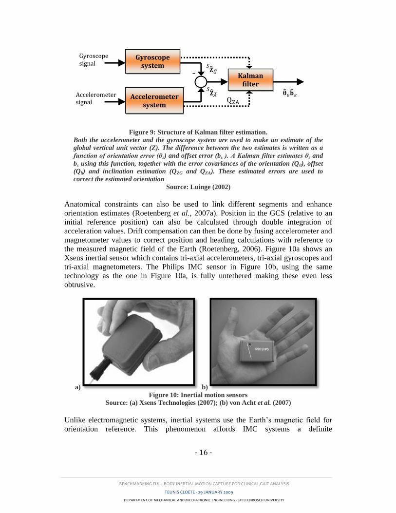
gyroscope drift. This is illustrated in Figure 9 (Luinge, 2002).
BENCHMARKING FULL-BODY INERTIAL MOTION CAPTURE FOR CLINICAL GAIT ANALYSIS
TEUNIS CLOETE - 29 JANUARY 2009
DEPARTMENT OF MECHANICAL AND MECHATRONIC ENGINEERING - STELLENBOSCH UNIVERSITY
- 16 -
Figure 9: Structure of Kalman filter estimation.
Both the accelerometer and the gyroscope system are used to make an estimate of the
global vertical unit vector (Z). The difference between the two estimates is written as a
function of orientation error (θε) and offset error (bε ). A Kalman filter estimates θε and
bε using this function, together with the error covariances of the orientation (Qθ), offset
(Qb) and inclination estimation (QZG and QZA). These estimated errors are used to
correct the estimated orientation
Source: Luinge (2002)
Anatomical constraints can also be used to link different segments and enhance
orientation estimates (Roetenberg et al., 2007a). Position in the GCS (relative to an
initial reference position) can also be calculated through double integration of
acceleration values. Drift compensation can then be done by fusing accelerometer and
magnetometer values to correct position and heading calculations with reference to
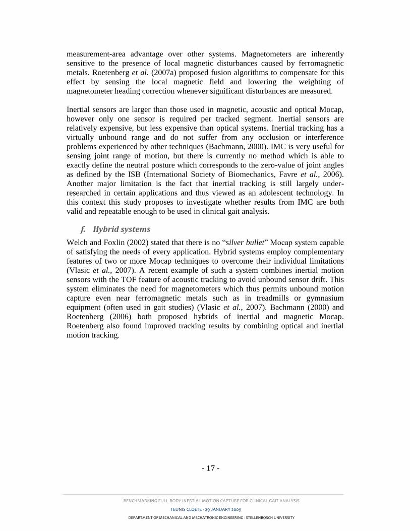
the measured magnetic field of the Earth (Roetenberg, 2006). Figure 10a shows an
Xsens inertial sensor which contains tri-axial accelerometers, tri-axial gyroscopes and
tri-axial magnetometers. The Philips IMC sensor in Figure 10b, using the same
technology as the one in Figure 10a, is fully untethered making these even less
obtrusive.
a) b)
Figure 10: Inertial motion sensors
Source: (a) Xsens Technologies (2007); (b) von Acht et al. (2007)
Unlike electromagnetic systems, inertial systems use the Earth’s magnetic field for
orientation reference. This phenomenon affords IMC systems a definite
Kalman filter
Accelerometer system
Gyroscope system
Gyroscope signal
Accelerometer signal
BENCHMARKING FULL-BODY INERTIAL MOTION CAPTURE FOR CLINICAL GAIT ANALYSIS
TEUNIS CLOETE - 29 JANUARY 2009
DEPARTMENT OF MECHANICAL AND MECHATRONIC ENGINEERING - STELLENBOSCH UNIVERSITY
- 17 -
measurement-area advantage over other systems. Magnetometers are inherently
sensitive to the presence of local magnetic disturbances caused by ferromagnetic
metals. Roetenberg et al. (2007a) proposed fusion algorithms to compensate for this
effect by sensing the local magnetic field and lowering the weighting of
magnetometer heading correction whenever significant disturbances are measured.
Inertial sensors are larger than those used in magnetic, acoustic and optical Mocap,
however only one sensor is required per tracked segment. Inertial sensors are
relatively expensive, but less expensive than optical systems. Inertial tracking has a
virtually unbound range and do not suffer from any occlusion or interference
problems experienced by other techniques (Bachmann, 2000). IMC is very useful for
sensing joint range of motion, but there is currently no method which is able to
exactly define the neutral posture which corresponds to the zero-value of joint angles
as defined by the ISB (International Society of Biomechanics, Favre et al., 2006).
Another major limitation is the fact that inertial tracking is still largely under-
researched in certain applications and thus viewed as an adolescent technology. In
this context this study proposes to investigate whether results from IMC are both
valid and repeatable enough to be used in clinical gait analysis.
f. Hybrid systems
Welch and Foxlin (2002) stated that there is no “silver bullet” Mocap system capable
of satisfying the needs of every application. Hybrid systems employ complementary
features of two or more Mocap techniques to overcome their individual limitations
(Vlasic et al., 2007). A recent example of such a system combines inertial motion
sensors with the TOF feature of acoustic tracking to avoid unbound sensor drift. This
system eliminates the need for magnetometers which thus permits unbound motion
capture even near ferromagnetic metals such as in treadmills or gymnasium
equipment (often used in gait studies) (Vlasic et al., 2007). Bachmann (2000) and
Roetenberg (2006) both proposed hybrids of inertial and magnetic Mocap.
Roetenberg also found improved tracking results by combining optical and inertial
motion tracking.
BENCHMARKING FULL-BODY INERTIAL MOTION CAPTURE FOR CLINICAL GAIT ANALYSIS
TEUNIS CLOETE - 29 JANUARY 2009
DEPARTMENT OF MECHANICAL AND MECHATRONIC ENGINEERING - STELLENBOSCH UNIVERSITY
- 18 -
g. Summary
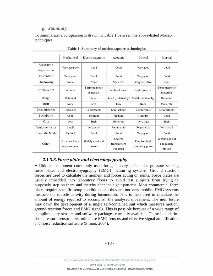
To summarize, a comparison is drawn in Table 1 between the above-listed Mocap
techniques:
Table 1: Summary of motion capture technologies
Mechanical Electromagnetic Acoustic Optical Inertial
Accuracy /
registration Very accurate Good Good Very good Good
Resolution Very good Good Good Very good Good
Shadowing None None Sensitive Very sensitive None
Interference Immune Ferromagnetic
materials Ambient noise Light sources
Ferromagnetic
materials
Range Unbound Small Small (In-lab only) Small (In-lab only) Unbound
Drift None Low Low None Moderate
Encumbrance Obtrusive Comfortable Comfortable Comfortable Comfortable
Sociability Good Medium Medium Medium Good
Cost Low High Moderate Very high High
Equipment size Small Very small Require lab Require lab Very small
Kinematic Model Limited Good Good Very good Good
Other Accurate force
measurement
Widely used and
proven
Several
transmitters
required
Requires high
computing power
Technology not
adequately
proven
2.1.3.3. Force plate and electromyography
Additional equipment commonly used for gait analysis includes pressure sensing
force plates and electromyography (EMG) measuring systems. Ground reaction
forces are used to calculate the moment and forces acting on joints. Force plates are
usually imbedded into laboratory floors to avoid test subjects from trying to
purposely step on them and thereby alter their gait patterns. Most commercial force
plates require specific setup conditions and thus are not very mobile. EMG systems
measure the muscle activity during locomotion. This is then used to calculate the
amount of energy required to accomplish the analysed movement. The near future
may dawn the development of a single self-contained suit which measures motion,
ground reaction forces and EMG signals. This is possible because of a wide range of
complimentary sensors and software packages currently available. These include in-
shoe pressure sensor units, miniature EMG sensors and effective signal amplification
and noise reduction software (Simon, 2004).
BENCHMARKING FULL-BODY INERTIAL MOTION CAPTURE FOR CLINICAL GAIT ANALYSIS
TEUNIS CLOETE - 29 JANUARY 2009
DEPARTMENT OF MECHANICAL AND MECHATRONIC ENGINEERING - STELLENBOSCH UNIVERSITY
- 19 -
2.2. Related research
2.2.1. Using motion capture for clinical gait analysis
The utilization of gait analysis in patient care was questioned by Simon (2004) who
cited findings by DeLuca, et al. (1997) showing that in a test of 91 children with
cerebral palsy, experienced clinicians changed their initial opinions in 52% of cases
after viewing quantitative gait analysis results. He still found gait analysis to lack
popularity.
According to measurements by Salarian et al. (2004) gait phases in PD patients
deviate significantly from able-bodied gait. They found that patients exhibit 52%
slower step velocity, 60% shorter step length, 40% longer gait cycle and 59% longer
double-stance than those with able-bodies. Han et al. (2006) found difficulty in
detecting gait in patients with PD. They also used only able-bodied subjects during
data acquisition. Lackovic et al. (2000) went further by using simplified gait cycle
analyses in distinguishing between able-bodied subjects and those with gait disorders.
In other studies such as those by Ebersbach et al. (1999) and Stolze et al. (2001),
attempts were made to use gait patterns to diagnose and/or distinguish between
certain movement disorders. Salarian et al. (2004) viewed the effect of deterioration
of gait patterns with increased progression of Parkinson’s disease. Finally, Lee et al.
(2000) went as far as to use a neural network combined with video analysis to
diagnose the presence of movement disorders. They employed only simple spatial
parameters and attained accurate diagnoses of between 82.5% and 85% for the patient
group. This study is still limited to only distinguishing between able-bodied persons
and those with movement abnormalities. Studies such as those by Han et al. (2006)
and Aminian et al. (2001) investigated autonomous gait cycle detection methods but
these studies do not give sufficient gait information for detecting more complex gait
abnormalities.
2.2.2. Verification of inertial motion capture
From studies conducted in the last decade it is apparent that IMC is continuously
evolving. Some researchers made use of gyroscopes alone to determine temporal and
spatial parameters (Aminian et al., 2001, Salarian et al., 2004). Salarian et al. (2004)
used their own peak detection algorithm to identify toe-off and heel-strike gait cycle
stages and a double pendulum anatomical model to determine the stride and step
lengths. Aminian et al. (2001) were only interested in temporal parameters and used
footswitches to correlate their results. They tested ten able-bodies subjects and ten
subjects with PD. Spatial parameters were normalized to height to test inter subject
variation. Han et al. (2006) found temporal parameters in PD patients using tri-axial
accelerometers. They achieved automated gait disorder detection accuracies in excess
of 90%.
BENCHMARKING FULL-BODY INERTIAL MOTION CAPTURE FOR CLINICAL GAIT ANALYSIS
TEUNIS CLOETE - 29 JANUARY 2009
DEPARTMENT OF MECHANICAL AND MECHATRONIC ENGINEERING - STELLENBOSCH UNIVERSITY
- 20 -
Accelerometers and gyroscopes were combined by Dejnabadi et al. (2005), Favre
(2006) and Luinge and Veltink (2005). Dejnabadi et al. (2005) proposed a new
method of estimating flexion angles. They created algorithms which eliminated the
need for integration in finding absolute joint angles in real time. Their results required
no filtering, were free from drift and made no cyclic assumptions. Compared to an
ultrasonic reference system (Zebris), their results showed excellent accuracy.
However, they only considered 2D sagittal plane knee angles which are the most
repeatable and easily measured of the nine lower-body joint angles. They furthered
their research by developing an algorithm in which accelerometer inclination
measurements were used to compensate for drift (Dejnabadi et al., 2006). As stated in
Section 2.1.3.2, accelerometers only sense inclination accurately when accelerations
are infinitesimal. For this reason they created a means of compensation correction
during the stance phase when accelerations are lowest and interpolation of the
compensation function during other gait cycle phases. They also found excellent
correlation with the ultrasonic reference system, but again only assessed knee flexion-
extension angles. Favre et al. (2006) went further by looking at 3D joint angles of the
knee. They used an electromagnetic Mocap system as reference (Polhemus Liberty®)
and found differences ranging from 1.2° to 12°. Again sagittal plane knee angles
showed the least difference. Luinge and Veltink (2005) used a Kalman filter to fuse
sensor types and compared their results with those obtained from using gyroscopes
alone. As expected, the Kalman filter significantly reduced the drift error found in
gyroscope readings. They used an optical Mocap system (Vicon) as baseline and
concluded that achieved accuracies were inadequate for applications where heading is
important.
Thies et al. (2007) investigated linear acceleration measurements from inertial
sensors during “reach and grasp” movements of two different manufacturers
compared to a Vicon (Oxford Metrics Ltd.) optical Mocap system. They found
exceptional correlations between all three systems which prove the repeatability and
validity of acceleration measurements. They also confirmed the existence of bias
errors due to misalignment of sensors and differences in calibration procedures. In
2000 Bachmann proposed a filter which used magnetometers and accelerometers to
determine orientation when movement frequency is low and gyroscopes for higher
frequency motion. It was tested for 2D motion and proved robust and accurate with
reference to results obtained using a Vicon system (Bachmann, 2000). Inertial sensors
have thus evolved to a point where drift-free tracking is possible using accelerometers
gyroscopes and magnetometers. As gait analysis is often conducted near
ferromagnetic materials such as in a gymnasium, it was necessary to come up with
solutions for subsequent drift errors. Roetenberg et al. (2007a) proposed a filter
which lowered such errors from 50° to 3.6°. They achieved this by lowering the
compensation weighting from magnetometers whenever the measured local magnetic
disturbances became significant. However this approach only remains valid for short
periods. Long term magnetic disturbances, such as those present when driving in a
BENCHMARKING FULL-BODY INERTIAL MOTION CAPTURE FOR CLINICAL GAIT ANALYSIS
TEUNIS CLOETE - 29 JANUARY 2009
DEPARTMENT OF MECHANICAL AND MECHATRONIC ENGINEERING - STELLENBOSCH UNIVERSITY
- 21 -
car, requires another solution. Vlasic et al. (2007) eliminated the need for
magnetometers by using ultrasonic sensors. These sensors use the measured absolute
distance between sensors to reduce orientation drift. This method showed great
promise but is still relatively untested.
2.2.3. Repeatability in gait patterns
Repeatability is one of the most important attributes of gait analysis equipment. In the
case of rehabilitation monitoring or intervention evaluation, a physician often looks at
relative gait parameter ranges as opposed to absolute angles, times or distances. Here
it is of paramount importance that an identical parameter, measured using an identical
test procedure, reflects the actual changes in that parameter without a significant
equipment measurement variability error. Several studies have looked at the
repeatability of gait patterns measure using an OMC system: (Yavuzer et al., 2006,
Besier et al., 2003, Mackey et al., 2005, Kadaba et al., 1989).
Mills et al. (2007) tested the within- and between-day repeatability and the inter- and
intra-tester repeatability of ten able-bodied adults using an electromagnetic Mocap
(EMC) system. Most of the above-mentioned studies used the approach presented by
Kadaba et al. (1989) to quantify temporal-spatial and joint angle repeatability.
Mackey et al. (2005) investigated the difference in gait repeatability between ten
able-bodied children and ten children with cerebral palsy. He used an optical Mocap
system and found acceptable and comparable and repeatability. In Section 4,
repeatability values obtained using the IMC system are compared to results obtained
by Kadaba et al. (1989) and Mills et al. (2005).
BENCHMARKING FULL-BODY INERTIAL MOTION CAPTURE FOR CLINICAL GAIT ANALYSIS
TEUNIS CLOETE - 29 JANUARY 2009
DEPARTMENT OF MECHANICAL AND MECHATRONIC ENGINEERING - STELLENBOSCH UNIVERSITY
- 22 -
3. VALIDITY STUDY
According to Favre, et al. (2006), no existing Mocap system produces sensor or
marker orientation measurements which exactly reflect the underlying bone
orientation. It is however important that the results from the chosen system
adequately exceeds the measuring error (Yavuzer et al., 2006). This concept is
evaluated in this section by comparing of results obtained by the IMC system gait
recording with those measured using a trusted OMC system.
3.1. Test participation
3.1.1. Inclusion criteria
Routine gait assessments were conducted on 14 able-bodied male subjects. Test
subjects were chosen under the condition that they do not suffer from any
neurological pathology and/or have not experienced any injury which may affect gait
function. Subjects were male and aged between 20 and 27 years. All the subjects
were fairly fit. This reduced the prevalence of sensor movement which was the main
concern when concurrently comparing the two systems.
3.1.2. Ethical approval / Protocol
Test subjects were used as controls in a separate study by Dr. Regan Arendse of the
faculty of Health Sciences at the University of Stellenbosch. Ethical approval was
obtained for this study. All subjects gave informed consent before being tested.
3.2. Apparatus
3.2.1. Vicon – Optical motion capture system
The Vicon OMC system (Oxford Metrics Ltd.) has been used for clinical gait analysis
for many years. It uses high-resolution, high-speed CMOS VICON cameras specially
designed for motion tracking. These cameras boast a resolution of up to 1280 × 1024
pixels and sampling rates of between 200 and 1000 Hz. Reflective markers are placed
on the objects (segments) to be tracked. Vicon Tracker software automatically
calculates the centres of each marker and reconstructs their position in the GCS.
Markers are combined to model the 3D spatial orientation and position of body
segments. This is usually accomplished in less than 7 ms. (Zhou and Hu, 2004)
In this study eight Vicon cameras were set up and calibrated within a 6 × 11 m
laboratory space. Reflective markers, of diameter 10 mm were used.
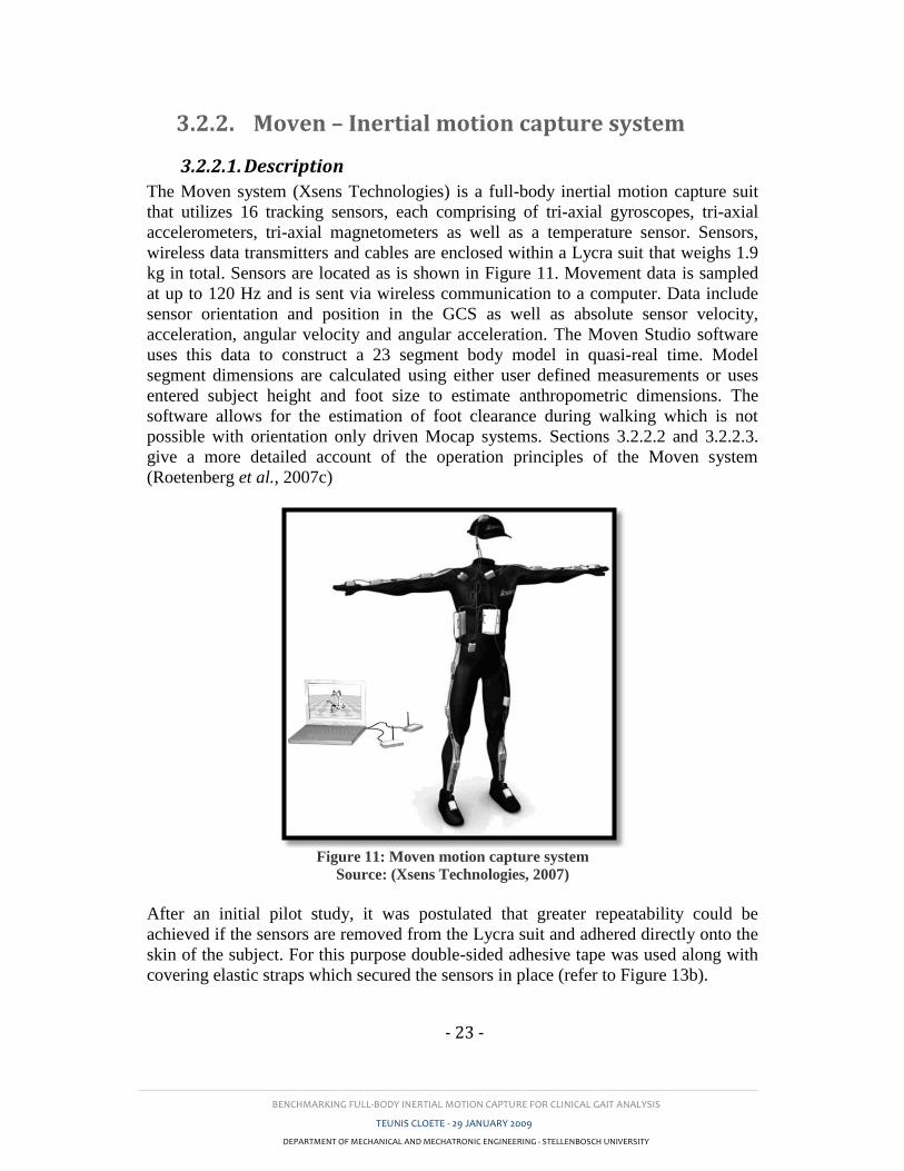
BENCHMARKING FULL-BODY INERTIAL MOTION CAPTURE FOR CLINICAL GAIT ANALYSIS
TEUNIS CLOETE - 29 JANUARY 2009
DEPARTMENT OF MECHANICAL AND MECHATRONIC ENGINEERING - STELLENBOSCH UNIVERSITY
- 23 -
3.2.2. Moven – Inertial motion capture system
3.2.2.1. Description
The Moven system (Xsens Technologies) is a full-body inertial motion capture suit
that utilizes 16 tracking sensors, each comprising of tri-axial gyroscopes, tri-axial
accelerometers, tri-axial magnetometers as well as a temperature sensor. Sensors,
wireless data transmitters and cables are enclosed within a Lycra suit that weighs 1.9
kg in total. Sensors are located as is shown in Figure 11. Movement data is sampled
at up to 120 Hz and is sent via wireless communication to a computer. Data include
sensor orientation and position in the GCS as well as absolute sensor velocity,
acceleration, angular velocity and angular acceleration. The Moven Studio software
uses this data to construct a 23 segment body model in quasi-real time. Model
segment dimensions are calculated using either user defined measurements or uses
entered subject height and foot size to estimate anthropometric dimensions. The
software allows for the estimation of foot clearance during walking which is not
possible with orientation only driven Mocap systems. Sections 3.2.2.2 and 3.2.2.3.
give a more detailed account of the operation principles of the Moven system
(Roetenberg et al., 2007c)
Figure 11: Moven motion capture system
Source: (Xsens Technologies, 2007)
After an initial pilot study, it was postulated that greater repeatability could be
achieved if the sensors are removed from the Lycra suit and adhered directly onto the
skin of the subject. For this purpose double-sided adhesive tape was used along with
covering elastic straps which secured the sensors in place (refer to Figure 13b).
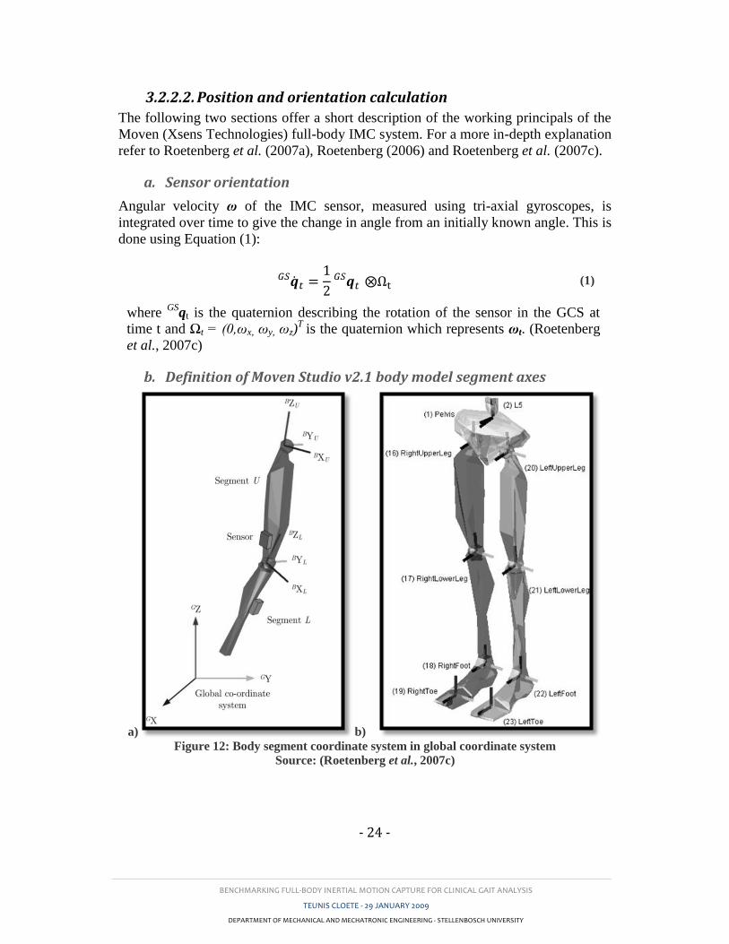
BENCHMARKING FULL-BODY INERTIAL MOTION CAPTURE FOR CLINICAL GAIT ANALYSIS
TEUNIS CLOETE - 29 JANUARY 2009
DEPARTMENT OF MECHANICAL AND MECHATRONIC ENGINEERING - STELLENBOSCH UNIVERSITY
- 24 -
3.2.2.2. Position and orientation calculation
The following two sections offer a short description of the working principals of the
Moven (Xsens Technologies) full-body IMC system. For a more in-depth explanation
refer to Roetenberg et al. (2007a), Roetenberg (2006) and Roetenberg et al. (2007c).
a. Sensor orientation
Angular velocity ω of the IMC sensor, measured using tri-axial gyroscopes, is
integrated over time to give the change in angle from an initially known angle. This is
done using Equation (1):
(1)
where GS
qt is the quaternion describing the rotation of the sensor in the GCS at
time t and Ωt = (0,ωx, ωy, ωz)T
is the quaternion which represents ωt. (Roetenberg
et al., 2007c)
b. Definition of Moven Studio v2.1 body model segment axes
a) b) Figure 12: Body segment coordinate system in global coordinate system
Source: (Roetenberg et al., 2007c)
BENCHMARKING FULL-BODY INERTIAL MOTION CAPTURE FOR CLINICAL GAIT ANALYSIS
TEUNIS CLOETE - 29 JANUARY 2009
DEPARTMENT OF MECHANICAL AND MECHATRONIC ENGINEERING - STELLENBOSCH UNIVERSITY
- 25 -
As shown in Figure 12, Moven Studio software defines the x-axis in the anterior-
posterior direction (anterior as positive), the y-axis in the medial-lateral direction (left
as positive) and the z-axis as vertically (up as positive). This is similar to the joint
coordinate system (described in Section 3.4.1) except that the x- and y-axes are
switched.
c. Sensor position
The position of the IMC sensor in the GCS (with reference to a calibrated starting
point) is calculated with the help of recordings from both linear accelerometers and
the gyroscopes used in orientation calculation. After removing the gravitational
component from acceleration signals using Equation (2) the sensor position in the
GCS is calculated by Equation (3).
(2)
(3)
where Gat and
Gg are the linear acceleration and gravity vectors in the GCS
respectively and pt is the position vector. (Roetenberg et al., 2007c)
d. Segment orientation and position
The body model, of which the lower body is depicted in Figure 12b, is comprised of
23 segments each considered as rigid bodies linked by joints. The sensors are
assumed to be rigidly attached to these segments.
The orientation of each segment is therefore assumed to be that of the corresponding
sensor with the exception of the spine, torso and toes which use a biomechanical
model to determine their orientation. Moven Studio defines contact points between
the body and the xy-plane of the GCS. These are used to determine the toe segment
orientations
Finding the position of each segment requires a bit more work. Because of sensor
drift it is necessary to limit the freedom of movement of each sensor relative to their
original calibration position. To accomplish this, segments are assumed to be joined
in a kinematic chain with the pelvis defined as the primary reference position. The
joint centres between proximal and distal segments now form the new reference
position for the distal segment. This joint centre position is calculated from the
proximal segment reference position, the segment (sensor) orientation and the
segment length (user-defined or anthropometrically calculated). This is achieved by
using Equation (4) below.
BENCHMARKING FULL-BODY INERTIAL MOTION CAPTURE FOR CLINICAL GAIT ANALYSIS
TEUNIS CLOETE - 29 JANUARY 2009
DEPARTMENT OF MECHANICAL AND MECHATRONIC ENGINEERING - STELLENBOSCH UNIVERSITY
- 26 -
(4)
where GpU1 and
GpU0 are the reference positions of the distal and proximal
segments at time t = 0. Here the orientation GB
qU and length sU of the proximal
segment U are known.
Because the segments considered are not in fact rigid bodies as is assumed by the
body model, statistical constraints are applied to avoid unlikely joint motions (e.g.
large varus-valgus of the knee). Each joint is constrained using its own characteristic
properties. (Roetenberg et al., 2007c)
3.2.2.3. Drift and magnetic interference compensation
The Moven IMC system uses complimentary sensor components and a Kalman filter
approach to correct propagating errors caused by sensor drift and/or magnetic field
interference. Using a Kalman filter update, joint position uncertainties are reduced by
correcting the drift. The sensor-noise, as well as statistical information about the joint
constraints is used to determine the Kalman gain. (Roetenberg et al., 2007c)
The segment orientation error is corrected by entering information about the heading
and gravitational vector components from magnetometers and accelerometers into a
Kalman filter. This is similar to the one illustrated in Figure 9 (refer to Section
2.1.3.2) which uses accelerometer measurements to correct orientation values.
According to Roetenberg et al. (2007c), local magnetic interferences from metallic
objects easily disturb the Earth’s magnetic field which in turn causes inaccurate
magnetometer readings. A compensation algorithm is therefore employed to reduce
these errors. This algorithm uses measurements of local magnetic disturbances to
reduce the weighting of the magnetometer component of the drift compensation filter.
This naturally increases the uncertainty of segment orientation calculations, but
according to a study by Roetenberg et al. (2007a), this method practically eliminated
the error caused by short term magnetic interferences.
3.3. Data acquisition and processing
3.3.1. Test protocol
Validity tests were conducted in a Mocap laboratory at the University of Cape Town,
in their Department of Sport Science. The following section discusses the procedure
followed during each gait assessment.
3.3.1.1. Sensor and marker application
Moven sensors were worn in a Lycra suit (Figure 13a) by 8 of the 14 test subjects.
For the remaining six subjects, sensors were applied using double-sided adhesive tape
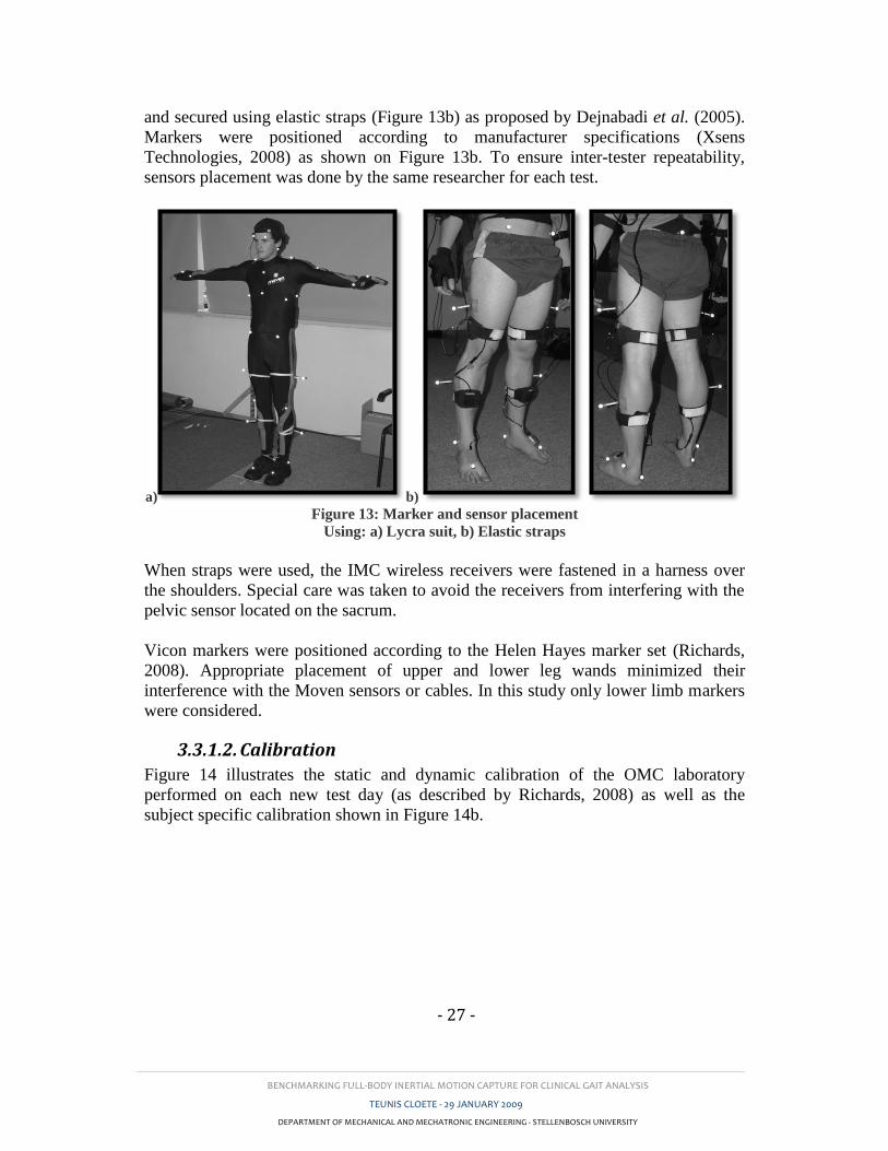
BENCHMARKING FULL-BODY INERTIAL MOTION CAPTURE FOR CLINICAL GAIT ANALYSIS
TEUNIS CLOETE - 29 JANUARY 2009
DEPARTMENT OF MECHANICAL AND MECHATRONIC ENGINEERING - STELLENBOSCH UNIVERSITY
- 27 -
and secured using elastic straps (Figure 13b) as proposed by Dejnabadi et al. (2005).
Markers were positioned according to manufacturer specifications (Xsens
Technologies, 2008) as shown on Figure 13b. To ensure inter-tester repeatability,
sensors placement was done by the same researcher for each test.
a) b) Figure 13: Marker and sensor placement
Using: a) Lycra suit, b) Elastic straps
When straps were used, the IMC wireless receivers were fastened in a harness over
the shoulders. Special care was taken to avoid the receivers from interfering with the
pelvic sensor located on the sacrum.
Vicon markers were positioned according to the Helen Hayes marker set (Richards,
2008). Appropriate placement of upper and lower leg wands minimized their
interference with the Moven sensors or cables. In this study only lower limb markers
were considered.
3.3.1.2. Calibration
Figure 14 illustrates the static and dynamic calibration of the OMC laboratory
performed on each new test day (as described by Richards, 2008) as well as the
subject specific calibration shown in Figure 14b.
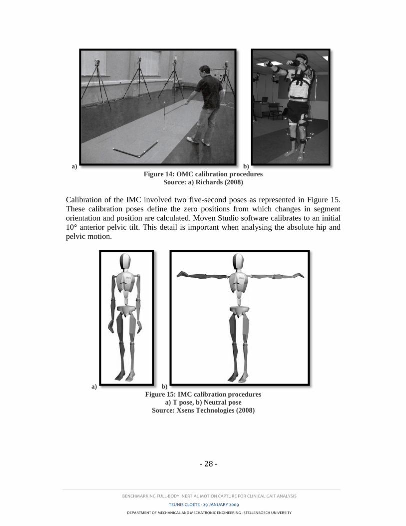
BENCHMARKING FULL-BODY INERTIAL MOTION CAPTURE FOR CLINICAL GAIT ANALYSIS
TEUNIS CLOETE - 29 JANUARY 2009
DEPARTMENT OF MECHANICAL AND MECHATRONIC ENGINEERING - STELLENBOSCH UNIVERSITY
- 28 -
a) b) Figure 14: OMC calibration procedures
Source: a) Richards (2008)
Calibration of the IMC involved two five-second poses as represented in Figure 15.
These calibration poses define the zero positions from which changes in segment
orientation and position are calculated. Moven Studio software calibrates to an initial
10° anterior pelvic tilt. This detail is important when analysing the absolute hip and
pelvic motion.
a) b) Figure 15: IMC calibration procedures
a) T pose, b) Neutral pose
Source: Xsens Technologies (2008)

BENCHMARKING FULL-BODY INERTIAL MOTION CAPTURE FOR CLINICAL GAIT ANALYSIS
TEUNIS CLOETE - 29 JANUARY 2009
DEPARTMENT OF MECHANICAL AND MECHATRONIC ENGINEERING - STELLENBOSCH UNIVERSITY
- 29 -
3.3.1.3. Procedure
Each gait assessment included the following steps:
1. Static calibration of the OMC system (Vicon)
2. Dynamic calibration of the OMC system
3. IMC (Moven) sensors applied to the subject (refer to 3.3.1.1)
4. Wires secured to avoid interference with OMC markers
5. OMC markers applied
6. Subject calibration of the OMC system
7. Subject calibration of the IMC system
8. Two unrecorded runs at a self-selected speed
9. Two runs recorded at a fast walking speed
10. Two runs recorded at a slow walking speed
11. Two runs recorded at a normal walking speed
12. Sensors and markers removed
Steps 3 to 12 were repeated for all test subjects tested on a single test day.
3.3.2. File format
IMC data was recorded in a proprietary *.MVN file format and converted to *.MVNx
file format which contains position and orientation data in ASCII format.
All kinematic data in the *.MVNx file is expressed in the global coordinates system
with the positive Z-axis defined as vertically up. The file contains calibration,
anthropometric scaling and recording setting information followed by a data matrix
which contains the orientation and position data of each segment for each sample
frame. This is illustrated on the abstract below taken from the Moven user manual:
Here GB
qseg is the quaternion vector (q0, q1, q2, q3) describing the rotation of the
segment in the global frame and Gposseg is the position vector (x,y,z) of the
segment from the origin in the global frame (Xsens Technologies, 2008).
OMC data was recorded in the more widely used *.C3D format. Gait data was
calculated within the Vicon software and exported in *.TXT format.
Sample 1 <F v=" GBqseg1 Gposseg1 GBqseg2 Gposseg2 …
GBqseg23 Gposseg23 " />
Sample 2 <F v=" GBqseg1 Gposseg1 GBqseg2 Gposseg2 …
GBqseg23 Gposseg23 " />
… Sample n <F v=" GBqseg1 Gposseg1 GBqseg2
Gposseg2 … GBqseg23
Gposseg23 " />
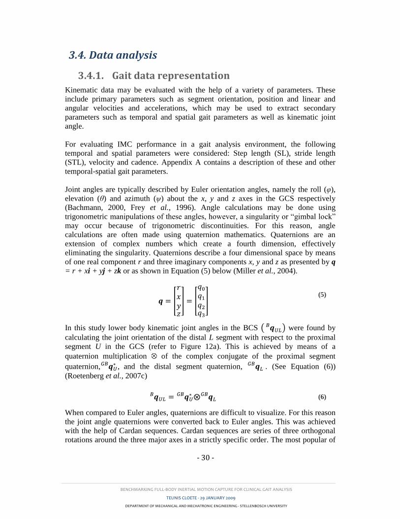
BENCHMARKING FULL-BODY INERTIAL MOTION CAPTURE FOR CLINICAL GAIT ANALYSIS
TEUNIS CLOETE - 29 JANUARY 2009
DEPARTMENT OF MECHANICAL AND MECHATRONIC ENGINEERING - STELLENBOSCH UNIVERSITY
- 30 -
3.4. Data analysis
3.4.1. Gait data representation
Kinematic data may be evaluated with the help of a variety of parameters. These
include primary parameters such as segment orientation, position and linear and
angular velocities and accelerations, which may be used to extract secondary
parameters such as temporal and spatial gait parameters as well as kinematic joint
angle.
For evaluating IMC performance in a gait analysis environment, the following
temporal and spatial parameters were considered: Step length (SL), stride length
(STL), velocity and cadence. Appendix A contains a description of these and other
temporal-spatial gait parameters.
Joint angles are typically described by Euler orientation angles, namely the roll (φ),
elevation (θ) and azimuth (ψ) about the x, y and z axes in the GCS respectively
(Bachmann, 2000, Frey et al., 1996). Angle calculations may be done using
trigonometric manipulations of these angles, however, a singularity or “gimbal lock”
may occur because of trigonometric discontinuities. For this reason, angle
calculations are often made using quaternion mathematics. Quaternions are an
extension of complex numbers which create a fourth dimension, effectively
eliminating the singularity. Quaternions describe a four dimensional space by means
of one real component r and three imaginary components x, y and z as presented by q
= r + xi + yj + zk or as shown in Equation (5) below (Miller et al., 2004).
(5)
In this study lower body kinematic joint angles in the BCS were found by
calculating the joint orientation of the distal L segment with respect to the proximal
segment U in the GCS (refer to Figure 12a). This is achieved by means of a
quaternion multiplication of the complex conjugate of the proximal segment
quaternion, ,
and the distal segment quaternion, . (See Equation (6))
(Roetenberg et al., 2007c)
(6)
When compared to Euler angles, quaternions are difficult to visualize. For this reason
the joint angle quaternions were converted back to Euler angles. This was achieved
with the help of Cardan sequences. Cardan sequences are series of three orthogonal
rotations around the three major axes in a strictly specific order. The most popular of

BENCHMARKING FULL-BODY INERTIAL MOTION CAPTURE FOR CLINICAL GAIT ANALYSIS
TEUNIS CLOETE - 29 JANUARY 2009
DEPARTMENT OF MECHANICAL AND MECHATRONIC ENGINEERING - STELLENBOSCH UNIVERSITY
- 31 -
these sequences is the Joint Coordinate System (JCS) proposed by Grood and Suntay
(1983) and used in the majority of gait research publications. If the axes are chosen
as: x – medial-lateral, y – anterior and z – up, then the JCS is defined as the sequence
xyz. Richards (2008) reported significant errors occurring when these sequences are
interchanged. It was therefore important to ensure that the same Cardan sequence was
used in IMC calculations as was employed by the OMC software.
The joint angles of the IMC system were therefore calculated using the JCS
(employed by the OMC software) with the aid of Equation (7) below as proposed by
Diebel (2006). These angles, representing rotations in the sagittal, frontal and
transverse planes, are used by most physicians or researchers to describe the gait of a
subject.
(7)
Here atan2 and asin are MATLAB (Mathworks, Natick, MA) commands for the
four quadrant inverse tangent and the inverse sine respectively.
Because of the difference in x- and y-axis definition between the JCS and that of the
IMC software, φ and ψ are then simply interchanged. The following joint angles
(Table 2) were calculated and used for both the validity and repeatability studies as
well as in training and testing a diagnostic neural network presented in Section 5.
Note the symbols in the first column as these are used in the result tables in later
sections: Table 2: Joint angles evaluated
Symbol Description Proximal segment Distal segment
φh
θh
ψh
Hip abduction-adduction
Hip flexion-extension
Hip internal-external rotation
Pelvis
(Sacral sensor)
Femur
(upper leg sensor)
φk
θk
ψk
Knee varus-valgus
Knee flexion-extension
Knee internal-external rotation
Femur
(upper leg sensor)
Tibia
(lower leg sensor)
φa
θa
ψa
Ankle eversion-inversion
Ankle plantar-dorsiflexion
Ankle supination-pronation
Tibia
(lower leg sensor)
Calcaneus and Metatarsal
(foot sensor)
φ, θ and ψ in Table 2 represent Euler angles in the frontal, sagittal and transverse
planes, respectively.
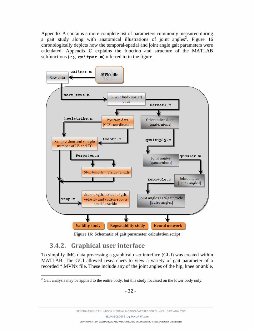
BENCHMARKING FULL-BODY INERTIAL MOTION CAPTURE FOR CLINICAL GAIT ANALYSIS
TEUNIS CLOETE - 29 JANUARY 2009
DEPARTMENT OF MECHANICAL AND MECHATRONIC ENGINEERING - STELLENBOSCH UNIVERSITY
- 32 -
Appendix A contains a more complete list of parameters commonly measured during
a gait study along with anatomical illustrations of joint angles2. Figure 16
chronologically depicts how the temporal-spatial and joint angle gait parameters were
calculated. Appendix C explains the function and structure of the MATLAB
subfunctions (e.g. gaitpar.m) referred to in the figure.
Figure 16: Schematic of gait parameter calculation script
3.4.2. Graphical user interface
To simplify IMC data processing a graphical user interface (GUI) was created within
MATLAB. The GUI allowed researchers to view a variety of gait parameter of a
recorded *.MVNx file. These include any of the joint angles of the hip, knee or ankle,
2 Gait analysis may be applied to the entire body, but this study focussed on the lower body only.
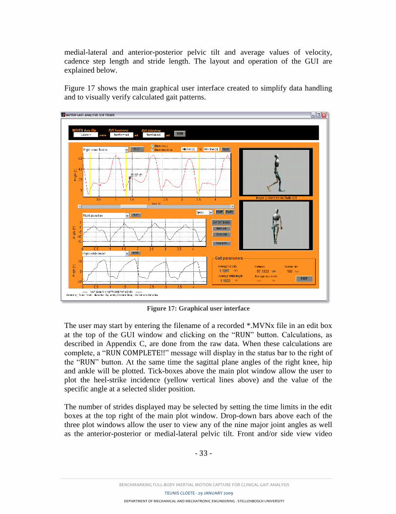
BENCHMARKING FULL-BODY INERTIAL MOTION CAPTURE FOR CLINICAL GAIT ANALYSIS
TEUNIS CLOETE - 29 JANUARY 2009
DEPARTMENT OF MECHANICAL AND MECHATRONIC ENGINEERING - STELLENBOSCH UNIVERSITY
- 33 -
medial-lateral and anterior-posterior pelvic tilt and average values of velocity,
cadence step length and stride length. The layout and operation of the GUI are
explained below.
Figure 17 shows the main graphical user interface created to simplify data handling
and to visually verify calculated gait patterns.
Figure 17: Graphical user interface
The user may start by entering the filename of a recorded *.MVNx file in an edit box
at the top of the GUI window and clicking on the “RUN” button. Calculations, as
described in Appendix C, are done from the raw data. When these calculations are
complete, a “RUN COMPLETE!!” message will display in the status bar to the right of
the “RUN” button. At the same time the sagittal plane angles of the right knee, hip
and ankle will be plotted. Tick-boxes above the main plot window allow the user to
plot the heel-strike incidence (yellow vertical lines above) and the value of the
specific angle at a selected slider position.
The number of strides displayed may be selected by setting the time limits in the edit
boxes at the top right of the main plot window. Drop-down bars above each of the
three plot windows allow the user to view any of the nine major joint angles as well
as the anterior-posterior or medial-lateral pelvic tilt. Front and/or side view video
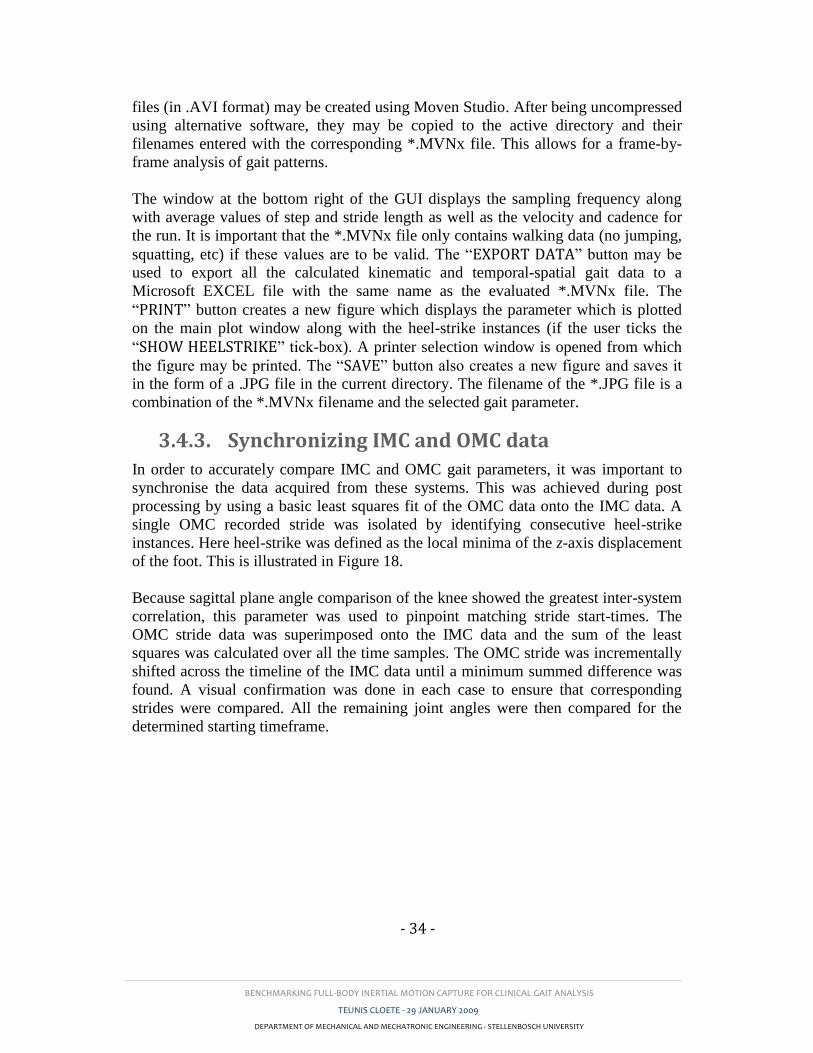
BENCHMARKING FULL-BODY INERTIAL MOTION CAPTURE FOR CLINICAL GAIT ANALYSIS
TEUNIS CLOETE - 29 JANUARY 2009
DEPARTMENT OF MECHANICAL AND MECHATRONIC ENGINEERING - STELLENBOSCH UNIVERSITY
- 34 -
files (in .AVI format) may be created using Moven Studio. After being uncompressed
using alternative software, they may be copied to the active directory and their
filenames entered with the corresponding *.MVNx file. This allows for a frame-by-
frame analysis of gait patterns.
The window at the bottom right of the GUI displays the sampling frequency along
with average values of step and stride length as well as the velocity and cadence for
the run. It is important that the *.MVNx file only contains walking data (no jumping,
squatting, etc) if these values are to be valid. The “EXPORT DATA” button may be
used to export all the calculated kinematic and temporal-spatial gait data to a
Microsoft EXCEL file with the same name as the evaluated *.MVNx file. The
“PRINT” button creates a new figure which displays the parameter which is plotted
on the main plot window along with the heel-strike instances (if the user ticks the
“SHOW HEELSTRIKE” tick-box). A printer selection window is opened from which
the figure may be printed. The “SAVE” button also creates a new figure and saves it
in the form of a .JPG file in the current directory. The filename of the *.JPG file is a
combination of the *.MVNx filename and the selected gait parameter.
3.4.3. Synchronizing IMC and OMC data
In order to accurately compare IMC and OMC gait parameters, it was important to
synchronise the data acquired from these systems. This was achieved during post
processing by using a basic least squares fit of the OMC data onto the IMC data. A
single OMC recorded stride was isolated by identifying consecutive heel-strike
instances. Here heel-strike was defined as the local minima of the z-axis displacement
of the foot. This is illustrated in Figure 18.
Because sagittal plane angle comparison of the knee showed the greatest inter-system
correlation, this parameter was used to pinpoint matching stride start-times. The
OMC stride data was superimposed onto the IMC data and the sum of the least
squares was calculated over all the time samples. The OMC stride was incrementally
shifted across the timeline of the IMC data until a minimum summed difference was
found. A visual confirmation was done in each case to ensure that corresponding
strides were compared. All the remaining joint angles were then compared for the
determined starting timeframe.
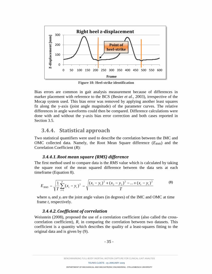
BENCHMARKING FULL-BODY INERTIAL MOTION CAPTURE FOR CLINICAL GAIT ANALYSIS
TEUNIS CLOETE - 29 JANUARY 2009
DEPARTMENT OF MECHANICAL AND MECHATRONIC ENGINEERING - STELLENBOSCH UNIVERSITY
- 35 -
Figure 18: Heel-strike identification
Bias errors are common in gait analysis measurement because of differences in
marker placement with reference to the BCS (Besier et al., 2003), irrespective of the
Mocap system used. This bias error was removed by applying another least squares
fit along the y-axis (joint angle magnitude) of the parameter curves. The relative
differences in angle waveforms could then be compared. Difference calculations were
done with and without the y-axis bias error correction and both cases reported in
Section 3.5.
3.4.4. Statistical approach
Two statistical quantifiers were used to describe the correlation between the IMC and
OMC collected data. Namely, the Root Mean Square difference (ERMS) and the
Correlation Coefficient (R):
3.4.4.1. Root mean square (RMS) difference
The first method used to compare data is the RMS value which is calculated by taking
the square root of the mean squared difference between the data sets at each
timeframe (Equation 8).
T
yxyxyxyx
TE tt
T
t
ttRMS
22
22
2
11
1
2 )(...)()()(
1
(8)
where xt and yt are the joint angle values (in degrees) of the IMC and OMC at time
frame t, respectively.
3.4.4.2. Coefficient of correlation
Weisstein (2008), proposed the use of a correlation coefficient (also called the cross-
correlation coefficient), R, in comparing the correlation between two datasets. This
coefficient is a quantity which describes the quality of a least-squares fitting to the
original data and is given by (9).
0
100
200
300
0 50 100 150 200 250 300 350 400 450 500 550 600
Z-d
isp
lace
me
nt
[mm
]
Frame
Right heel z-displacement
Point of heel-strike
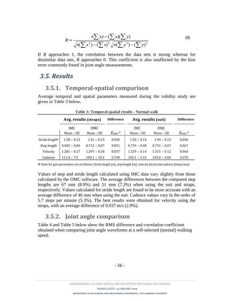
BENCHMARKING FULL-BODY INERTIAL MOTION CAPTURE FOR CLINICAL GAIT ANALYSIS
TEUNIS CLOETE - 29 JANUARY 2009
DEPARTMENT OF MECHANICAL AND MECHATRONIC ENGINEERING - STELLENBOSCH UNIVERSITY
- 36 -
2222 )()()()(
))((
yynxxn
yxxynR
(9)
If R approaches 1, the correlation between the data sets is strong whereas for
dissimilar data sets, R approaches 0. This coefficient is also unaffected by the bias
error commonly found in joint angle measurements.
3.5. Results
3.5.1. Temporal-spatial comparison
Average temporal and spatial parameters measured during the validity study are
given in Table 3 below.
Table 3: Temporal-spatial results - Normal walk
Avg. results (straps) Difference Avg. results (suit) Difference
IMC OMC
IMC OMC
Mean ± SD Mean ± SD ERMS # Mean ± SD Mean ± SD ERMS #
Stride length# 1.38 ± 0.12 1.41 ± 0.13
0.045 1.50 ± 0.14 1.49 ± 0.13
0.046
Step length 0.685 ± 0.06 0.713 ± 0.07
0.051 0.759 ± 0.08 0.751 ± 0.07
0.067
Velocity 1.281 ± 0.17 1.297 ± 0.18
0.037 1.329 ± 0.14 1.315 ± 0.12
0.060
Cadence 111.9 ± 7.5 109.1 ± 10.1
5.749 105.1 ± 5.15 105.0 ± 4.00
5.670
# Units for gait parameters are as follows: Stride length [m], step length [m], velocity [m/s] and cadence [steps/min]
Values of step and stride length calculated using IMC data vary slightly from those
calculated by the OMC software. The average differences between the compared step
lengths are 67 mm (8.9%) and 51 mm (7.3%) when using the suit and straps,
respectively. Values calculated for stride length are found to be more accurate with an
average difference of 46 mm when using the suit. Cadence values vary in the order of
5.7 steps per minute (5.3%). The best results were obtained for velocity using the
straps, with an average difference of 0.037 m/s (2.9%).
3.5.2. Joint angle comparison
Table 4 and Table 5 below show the RMS difference and correlation coefficient
obtained when comparing joint angle waveforms at a self-selected (normal) walking
speed.
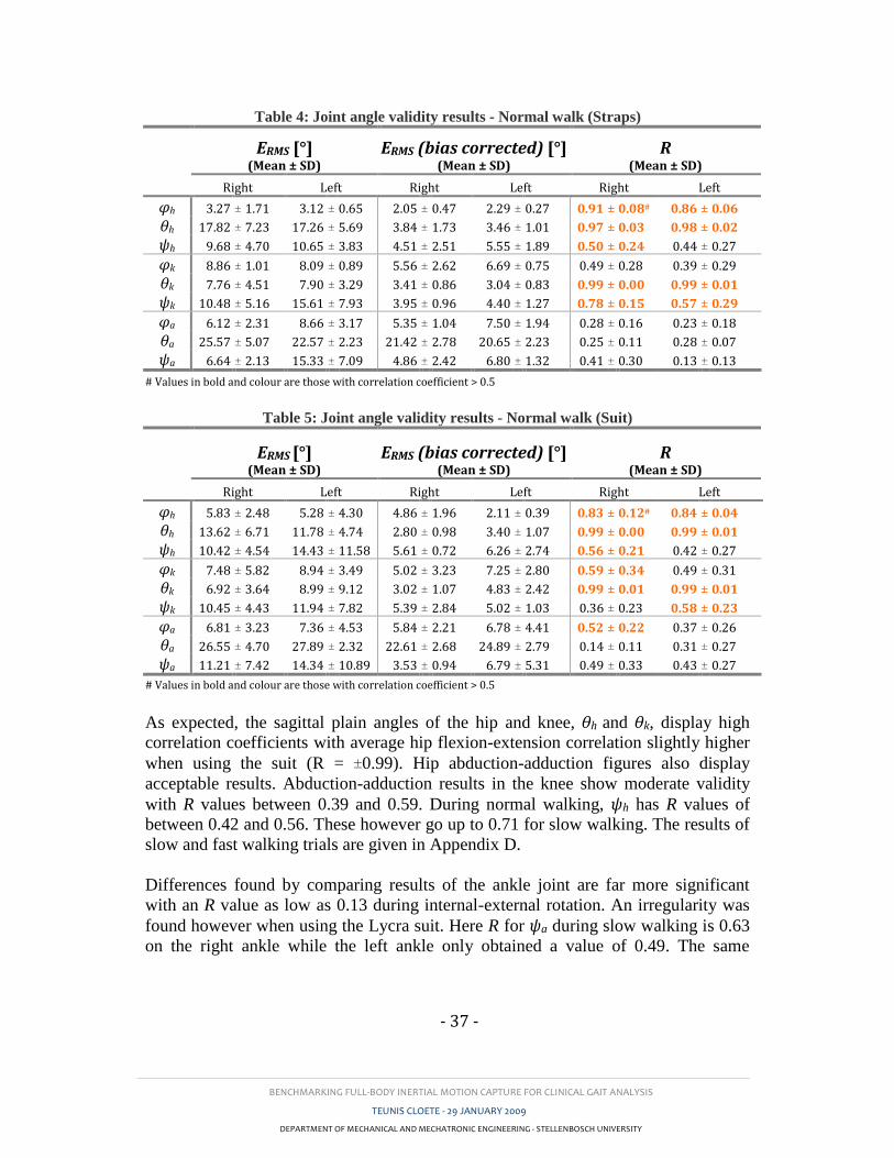
BENCHMARKING FULL-BODY INERTIAL MOTION CAPTURE FOR CLINICAL GAIT ANALYSIS
TEUNIS CLOETE - 29 JANUARY 2009
DEPARTMENT OF MECHANICAL AND MECHATRONIC ENGINEERING - STELLENBOSCH UNIVERSITY
- 37 -
Table 4: Joint angle validity results - Normal walk (Straps)
ERMS [°] (Mean ± SD)
ERMS (bias corrected) [°] (Mean ± SD)
R (Mean ± SD)
Right Left Right Left Right Left
φh 3.27 ± 1.71 3.12 ± 0.65 2.05 ± 0.47 2.29 ± 0.27 0.91 ± 0.08# 0.86 ± 0.06
θh 17.82 ± 7.23 17.26 ± 5.69 3.84 ± 1.73 3.46 ± 1.01 0.97 ± 0.03 0.98 ± 0.02
ψh 9.68 ± 4.70 10.65 ± 3.83 4.51 ± 2.51 5.55 ± 1.89 0.50 ± 0.24 0.44 ± 0.27
φk 8.86 ± 1.01 8.09 ± 0.89 5.56 ± 2.62 6.69 ± 0.75 0.49 ± 0.28 0.39 ± 0.29
θk 7.76 ± 4.51 7.90 ± 3.29 3.41 ± 0.86 3.04 ± 0.83 0.99 ± 0.00 0.99 ± 0.01
ψk 10.48 ± 5.16 15.61 ± 7.93 3.95 ± 0.96 4.40 ± 1.27 0.78 ± 0.15 0.57 ± 0.29
φa 6.12 ± 2.31 8.66 ± 3.17 5.35 ± 1.04 7.50 ± 1.94 0.28 ± 0.16 0.23 ± 0.18
θa 25.57 ± 5.07 22.57 ± 2.23 21.42 ± 2.78 20.65 ± 2.23 0.25 ± 0.11 0.28 ± 0.07
ψa 6.64 ± 2.13 15.33 ± 7.09 4.86 ± 2.42 6.80 ± 1.32 0.41 ± 0.30 0.13 ± 0.13
# Values in bold and colour are those with correlation coefficient > 0.5
Table 5: Joint angle validity results - Normal walk (Suit)
ERMS [°] (Mean ± SD)
ERMS (bias corrected) [°] (Mean ± SD)
R (Mean ± SD)
Right Left Right Left Right Left
φh 5.83 ± 2.48 5.28 ± 4.30 4.86 ± 1.96 2.11 ± 0.39 0.83 ± 0.12# 0.84 ± 0.04
θh 13.62 ± 6.71 11.78 ± 4.74 2.80 ± 0.98 3.40 ± 1.07 0.99 ± 0.00 0.99 ± 0.01
ψh 10.42 ± 4.54 14.43 ± 11.58 5.61 ± 0.72 6.26 ± 2.74 0.56 ± 0.21 0.42 ± 0.27
φk 7.48 ± 5.82 8.94 ± 3.49 5.02 ± 3.23 7.25 ± 2.80 0.59 ± 0.34 0.49 ± 0.31
θk 6.92 ± 3.64 8.99 ± 9.12 3.02 ± 1.07 4.83 ± 2.42 0.99 ± 0.01 0.99 ± 0.01
ψk 10.45 ± 4.43 11.94 ± 7.82 5.39 ± 2.84 5.02 ± 1.03 0.36 ± 0.23 0.58 ± 0.23
φa 6.81 ± 3.23 7.36 ± 4.53 5.84 ± 2.21 6.78 ± 4.41 0.52 ± 0.22 0.37 ± 0.26
θa 26.55 ± 4.70 27.89 ± 2.32 22.61 ± 2.68 24.89 ± 2.79 0.14 ± 0.11 0.31 ± 0.27
ψa 11.21 ± 7.42 14.34 ± 10.89 3.53 ± 0.94 6.79 ± 5.31 0.49 ± 0.33 0.43 ± 0.27
# Values in bold and colour are those with correlation coefficient > 0.5
As expected, the sagittal plain angles of the hip and knee, θh and θk, display high
correlation coefficients with average hip flexion-extension correlation slightly higher
when using the suit (R = ±0.99). Hip abduction-adduction figures also display
acceptable results. Abduction-adduction results in the knee show moderate validity
with R values between 0.39 and 0.59. During normal walking, ψh has R values of
between 0.42 and 0.56. These however go up to 0.71 for slow walking. The results of
slow and fast walking trials are given in Appendix D.
Differences found by comparing results of the ankle joint are far more significant
with an R value as low as 0.13 during internal-external rotation. An irregularity was
found however when using the Lycra suit. Here R for ψa during slow walking is 0.63
on the right ankle while the left ankle only obtained a value of 0.49. The same
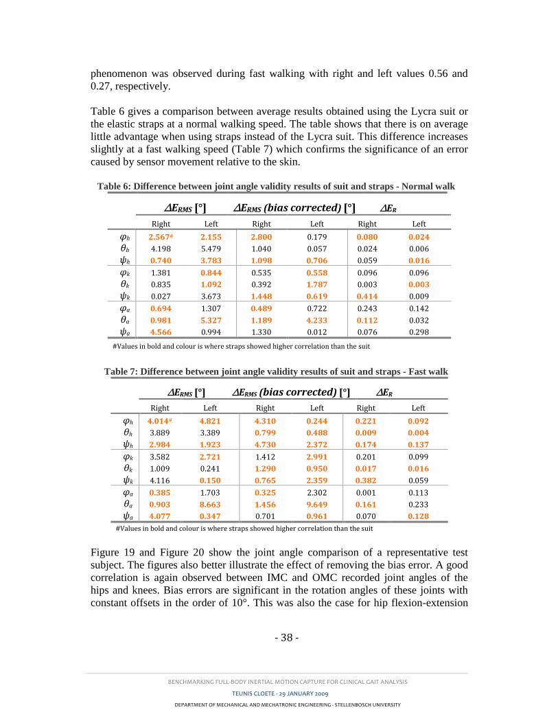
BENCHMARKING FULL-BODY INERTIAL MOTION CAPTURE FOR CLINICAL GAIT ANALYSIS
TEUNIS CLOETE - 29 JANUARY 2009
DEPARTMENT OF MECHANICAL AND MECHATRONIC ENGINEERING - STELLENBOSCH UNIVERSITY
- 38 -
phenomenon was observed during fast walking with right and left values 0.56 and
0.27, respectively.
Table 6 gives a comparison between average results obtained using the Lycra suit or
the elastic straps at a normal walking speed. The table shows that there is on average
little advantage when using straps instead of the Lycra suit. This difference increases
slightly at a fast walking speed (Table 7) which confirms the significance of an error
caused by sensor movement relative to the skin.
Table 6: Difference between joint angle validity results of suit and straps - Normal walk
∆ERMS [°] ∆ERMS (bias corrected) [°] ∆ER
Right Left Right Left Right Left
φh 2.567# 2.155 2.800 0.179 0.080 0.024
θh 4.198 5.479 1.040 0.057 0.024 0.006
ψh 0.740 3.783 1.098 0.706 0.059 0.016
φk 1.381 0.844 0.535 0.558 0.096 0.096
θk 0.835 1.092 0.392 1.787 0.003 0.003
ψk 0.027 3.673 1.448 0.619 0.414 0.009
φa 0.694 1.307 0.489 0.722 0.243 0.142
θa 0.981 5.327 1.189 4.233 0.112 0.032
ψa 4.566 0.994 1.330 0.012 0.076 0.298
#Values in bold and colour is where straps showed higher correlation than the suit
Table 7: Difference between joint angle validity results of suit and straps - Fast walk
∆ERMS [°] ∆ERMS (bias corrected) [°] ∆ER
Right Left Right Left Right Left
φh 4.014# 4.821 4.310 0.244 0.221 0.092
θh 3.889 3.389 0.799 0.488 0.009 0.004
ψh 2.984 1.923 4.730 2.372 0.174 0.137
φk 3.582 2.721 1.412 2.991 0.201 0.099
θk 1.009 0.241 1.290 0.950 0.017 0.016
ψk 4.116 0.150 0.765 2.359 0.382 0.059
φa 0.385 1.703 0.325 2.302 0.001 0.113
θa 0.903 8.663 1.456 9.649 0.161 0.233
ψa 4.077 0.347 0.701 0.961 0.070 0.128
#Values in bold and colour is where straps showed higher correlation than the suit
Figure 19 and Figure 20 show the joint angle comparison of a representative test
subject. The figures also better illustrate the effect of removing the bias error. A good
correlation is again observed between IMC and OMC recorded joint angles of the
hips and knees. Bias errors are significant in the rotation angles of these joints with
constant offsets in the order of 10°. This was also the case for hip flexion-extension
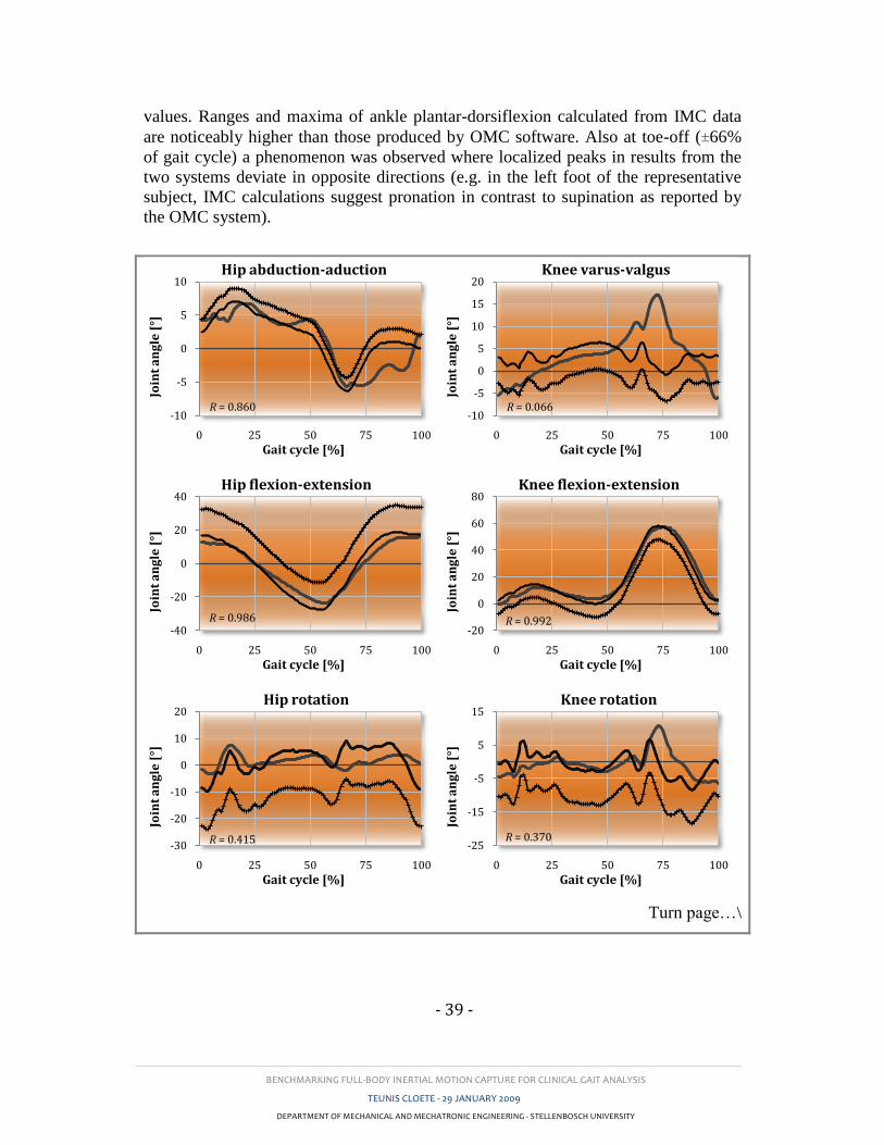
BENCHMARKING FULL-BODY INERTIAL MOTION CAPTURE FOR CLINICAL GAIT ANALYSIS
TEUNIS CLOETE - 29 JANUARY 2009
DEPARTMENT OF MECHANICAL AND MECHATRONIC ENGINEERING - STELLENBOSCH UNIVERSITY
- 39 -
values. Ranges and maxima of ankle plantar-dorsiflexion calculated from IMC data
are noticeably higher than those produced by OMC software. Also at toe-off (±66%
of gait cycle) a phenomenon was observed where localized peaks in results from the
two systems deviate in opposite directions (e.g. in the left foot of the representative
subject, IMC calculations suggest pronation in contrast to supination as reported by
the OMC system).
Turn page…\
-10
-5
0
5
10
0 25 50 75 100
Join
t a
ng
le [
°]
Gait cycle [%]
Hip abduction-aduction
R = 0.860 -10
-5
0
5
10
15
20
0 25 50 75 100
Join
t a
ng
le [
°]Gait cycle [%]
Knee varus-valgus
R = 0.066
-40
-20
0
20
40
0 25 50 75 100
Join
t a
ng
le [
°]
Gait cycle [%]
Hip flexion-extension
R = 0.986 -20
0
20
40
60
80
0 25 50 75 100
Join
t a
ng
le [
°]
Gait cycle [%]
Knee flexion-extension
R = 0.992
-30
-20
-10
0
10
20
0 25 50 75 100
Join
t a
ng
le [
°]
Gait cycle [%]
Hip rotation
R = 0.415 -25
-15
-5
5
15
0 25 50 75 100
Join
t a
ng
le [
°]
Gait cycle [%]
Knee rotation
R = 0.370
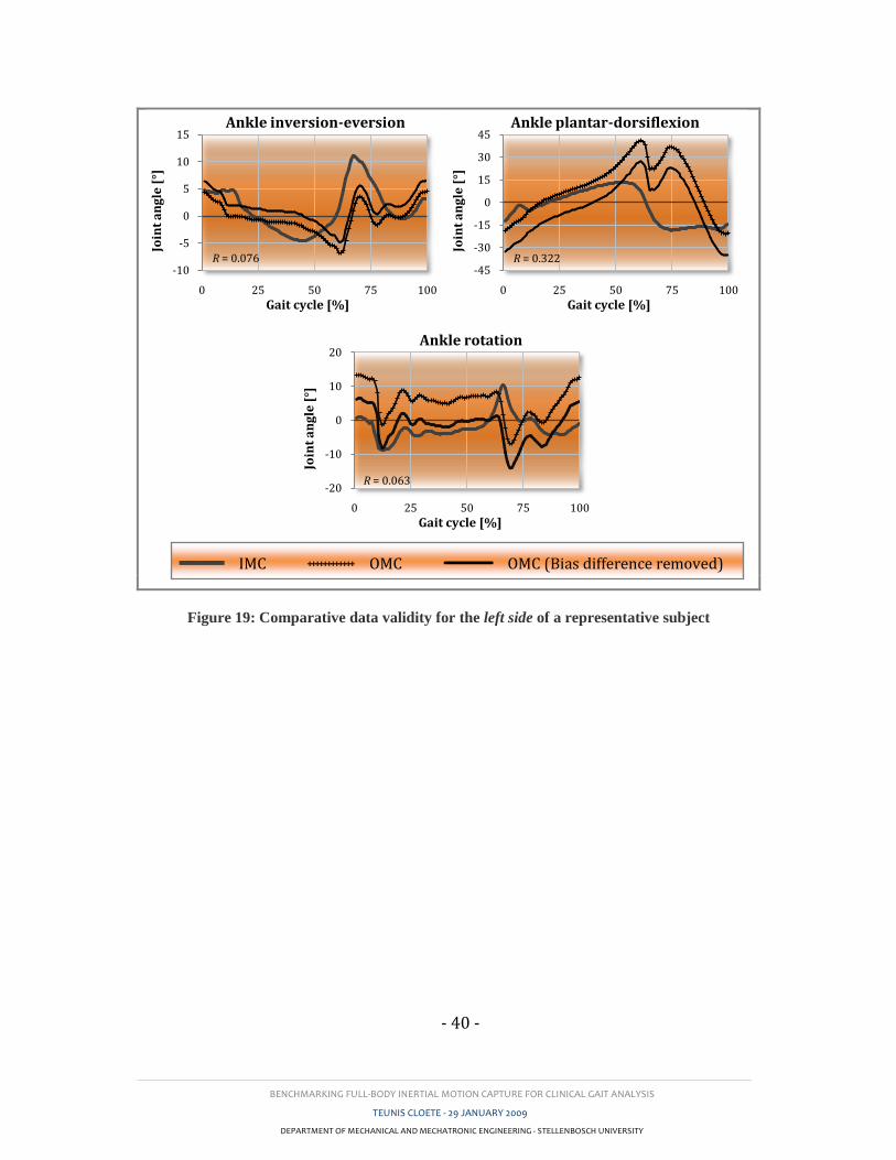
BENCHMARKING FULL-BODY INERTIAL MOTION CAPTURE FOR CLINICAL GAIT ANALYSIS
TEUNIS CLOETE - 29 JANUARY 2009
DEPARTMENT OF MECHANICAL AND MECHATRONIC ENGINEERING - STELLENBOSCH UNIVERSITY
- 40 -
Figure 19: Comparative data validity for the left side of a representative subject
-10
-5
0
5
10
15
0 25 50 75 100
Join
t a
ng
le [
°]
Gait cycle [%]
Ankle inversion-eversion
R = 0.076 -45
-30
-15
0
15
30
45
0 25 50 75 100
Join
t a
ng
le [
°]
Gait cycle [%]
Ankle plantar-dorsiflexion
R = 0.322
-20
-10
0
10
20
0 25 50 75 100
Join
t a
ng
le [
°]
Gait cycle [%]
Ankle rotation
R = 0.063
IMC ++++++++++++ OMC OMC (Bias difference removed)
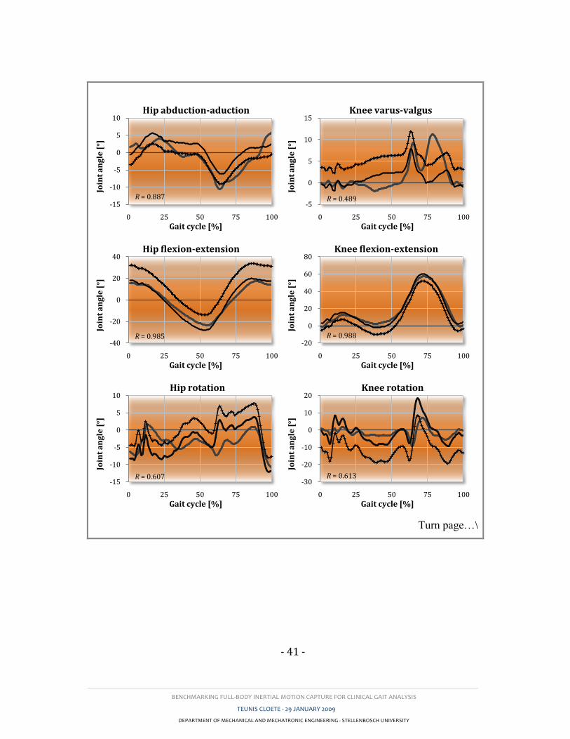
BENCHMARKING FULL-BODY INERTIAL MOTION CAPTURE FOR CLINICAL GAIT ANALYSIS
TEUNIS CLOETE - 29 JANUARY 2009
DEPARTMENT OF MECHANICAL AND MECHATRONIC ENGINEERING - STELLENBOSCH UNIVERSITY
- 41 -
Turn page…\
-15
-10
-5
0
5
10
0 25 50 75 100
Join
t a
ng
le [
°]
Gait cycle [%]
Hip abduction-aduction
R = 0.887 -5
0
5
10
15
0 25 50 75 100
Join
t a
ng
le [
°]
Gait cycle [%]
Knee varus-valgus
R = 0.489
-40
-20
0
20
40
0 25 50 75 100
Join
t a
ng
le [
°]
Gait cycle [%]
Hip flexion-extension
R = 0.985 -20
0
20
40
60
80
0 25 50 75 100
Join
t a
ng
le [
°]
Gait cycle [%]
Knee flexion-extension
R = 0.988
-15
-10
-5
0
5
10
0 25 50 75 100
Join
t a
ng
le [
°]
Gait cycle [%]
Hip rotation
R = 0.607 -30
-20
-10
0
10
20
0 25 50 75 100
Join
t a
ng
le [
°]
Gait cycle [%]
Knee rotation
R = 0.613
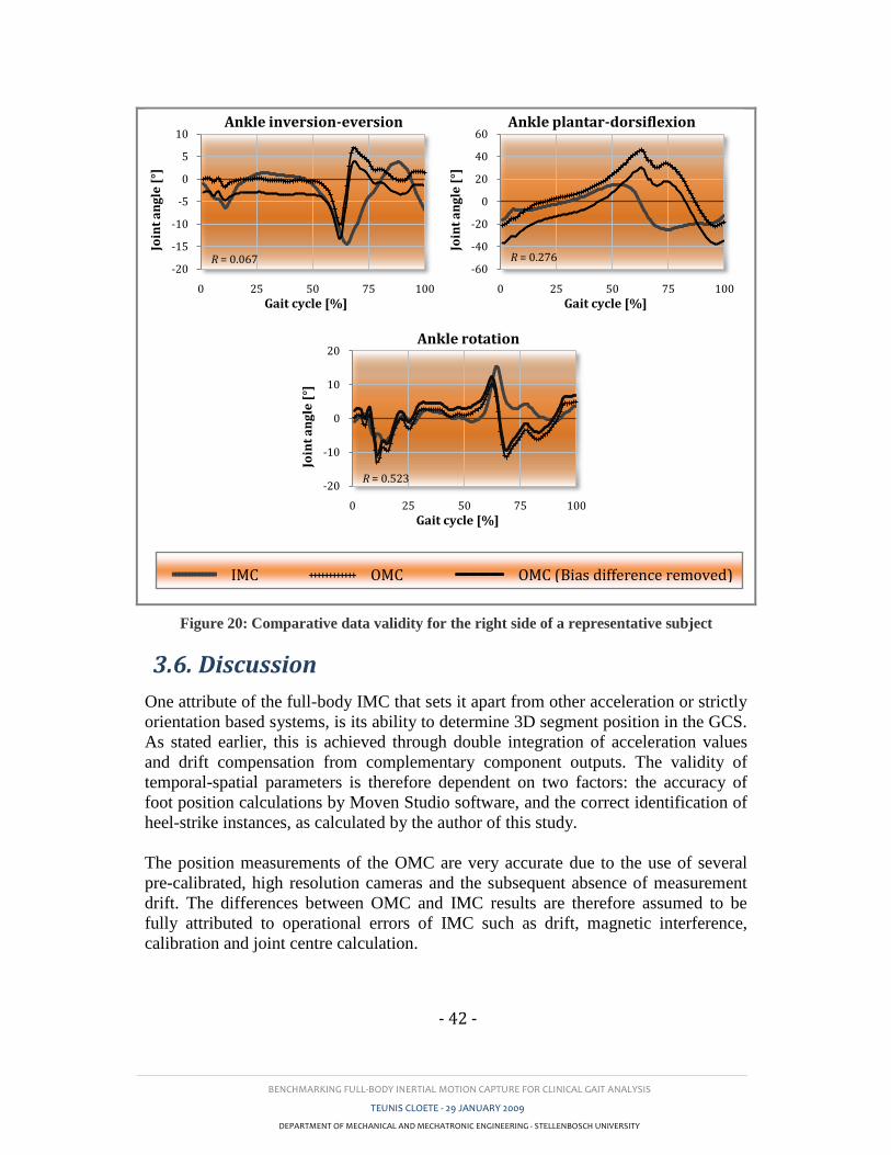
BENCHMARKING FULL-BODY INERTIAL MOTION CAPTURE FOR CLINICAL GAIT ANALYSIS
TEUNIS CLOETE - 29 JANUARY 2009
DEPARTMENT OF MECHANICAL AND MECHATRONIC ENGINEERING - STELLENBOSCH UNIVERSITY
- 42 -
Figure 20: Comparative data validity for the right side of a representative subject
3.6. Discussion
One attribute of the full-body IMC that sets it apart from other acceleration or strictly
orientation based systems, is its ability to determine 3D segment position in the GCS.
As stated earlier, this is achieved through double integration of acceleration values
and drift compensation from complementary component outputs. The validity of
temporal-spatial parameters is therefore dependent on two factors: the accuracy of
foot position calculations by Moven Studio software, and the correct identification of
heel-strike instances, as calculated by the author of this study.
The position measurements of the OMC are very accurate due to the use of several
pre-calibrated, high resolution cameras and the subsequent absence of measurement
drift. The differences between OMC and IMC results are therefore assumed to be
fully attributed to operational errors of IMC such as drift, magnetic interference,
calibration and joint centre calculation.
-20
-15
-10
-5
0
5
10
0 25 50 75 100
Join
t a
ng
le [
°]
Gait cycle [%]
Ankle inversion-eversion
R = 0.067 -60
-40
-20
0
20
40
60
0 25 50 75 100
Join
t a
ng
le [
°]
Gait cycle [%]
Ankle plantar-dorsiflexion
R = 0.276
-20
-10
0
10
20
0 25 50 75 100
Join
t a
ng
le [
°]
Gait cycle [%]
Ankle rotation
R = 0.523
IMC ++++++++++++ OMC OMC (Bias difference removed)
BENCHMARKING FULL-BODY INERTIAL MOTION CAPTURE FOR CLINICAL GAIT ANALYSIS
TEUNIS CLOETE - 29 JANUARY 2009
DEPARTMENT OF MECHANICAL AND MECHATRONIC ENGINEERING - STELLENBOSCH UNIVERSITY
- 43 -
Velocity was calculated using the total distance displaced by the pelvic sensor
divided by the time between consecutive heel-strike instances of one side (over one
stride). This value therefore indicates the average velocity between two positional
points in time and is therefore considered good indication of the position validity of
Moven Studio results.
As discussed in Appendix C, step and stride length calculations relied upon the
definition of a direction vector. Step lengths were calculated as the vector
components parallel to the direction vector, whereas stride length utilized the absolute
distance between foot coordinates at consecutive heel-strike instances. Lower average
differences of stride length (Straps: 3.2%, Suit: 4.5%) to step length (Straps: 8.9%,
Suit: 7.3%) indicate that position calculations are acceptable and that the directional
vector approach of calculating step length requires refinement. Even with the current
software, however, the temporal-spatial parameters show acceptable validity.
Besier et al. (2003) cited Della Croce et al. (1999) in saying that the errors associated
with the imprecise location of anatomical landforms (ALs) are noted to be the
greatest source of error in motion analysis compared to instrument error and skin
artefacts. Whether it is the inaccurate positioning of markers or the miscalculation of
joint centres, this is the case for all motion analysis systems. Besier et al. (2003) went
on to state that the greatest error in AL location occurs in the foot. This was
confirmed by the validity results in Section 3.5.2. Unlike with temporal-spatial
parameters, the OMC values also suffer from errors such as marker vibration and
inertia (especially in the wands). Keeping this in mind, the OMC was still considered
as the “golden standard” because of its widespread use and acceptance.
High correlation values in sagittal joint angles were found in the hips and knees. This
suggests that the validity of joint angles, calculated from IMC data, may be affected
by the rotational freedom of the joint around non-primary rotation axes and/or the
range of motion around the primary axis, as both these characteristics are more
prevalent in sagittal plane angles. Acceptable correlation values were recorded for hip
and knee abduction-adduction. Differences may stem from a misalignment of IMC
sensors or inaccurate positioning of OMC markers leading to mismatched rotation
centres or axes. A higher R value for knee rotation during slow walking suggests that
sensor or marker movement relative to the BCS adds to errors in this plane.
Low correlation values in the ankle joints could be as a result of the following
factors:
o Incorrect allocation or calculation of angle axes (e.g. the OMC software uses a
marker on the lateral malleoli and an estimation based on a measured ankle
width to calculate the sagittal plane angle of the ankle, while the IMC
software uses an axis defined during static calibration).
o Movement of the IMC sensor on the soft tissue on top of the foot.
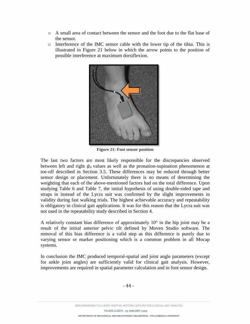
BENCHMARKING FULL-BODY INERTIAL MOTION CAPTURE FOR CLINICAL GAIT ANALYSIS
TEUNIS CLOETE - 29 JANUARY 2009
DEPARTMENT OF MECHANICAL AND MECHATRONIC ENGINEERING - STELLENBOSCH UNIVERSITY
- 44 -
o A small area of contact between the sensor and the foot due to the flat base of
the sensor.
o Interference of the IMC sensor cable with the lower tip of the tibia. This is
illustrated in Figure 21 below in which the arrow points to the position of
possible interference at maximum dorsiflexion.
Figure 21: Foot sensor position
The last two factors are most likely responsible for the discrepancies observed
between left and right ψa values as well as the pronation-supination phenomenon at
toe-off described in Section 3.5. These differences may be reduced through better
sensor design or placement. Unfortunately there is no means of determining the
weighting that each of the above-mentioned factors had on the total difference. Upon
studying Table 6 and Table 7, the initial hypothesis of using double-sided tape and
straps in instead of the Lycra suit was confirmed by the slight improvements in
validity during fast walking trials. The highest achievable accuracy and repeatability
is obligatory in clinical gait applications. It was for this reason that the Lycra suit was
not used in the repeatability study described in Section 4.
A relatively constant bias difference of approximately 10° in the hip joint may be a
result of the initial anterior pelvic tilt defined by Moven Studio software. The
removal of this bias difference is a valid step as this difference is purely due to
varying sensor or marker positioning which is a common problem in all Mocap
systems.
In conclusion the IMC produced temporal-spatial and joint angle parameters (except
for ankle joint angles) are sufficiently valid for clinical gait analysis. However,
improvements are required in spatial parameter calculation and in foot sensor design.
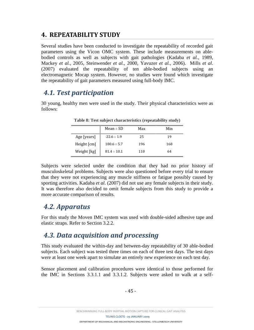
BENCHMARKING FULL-BODY INERTIAL MOTION CAPTURE FOR CLINICAL GAIT ANALYSIS
TEUNIS CLOETE - 29 JANUARY 2009
DEPARTMENT OF MECHANICAL AND MECHATRONIC ENGINEERING - STELLENBOSCH UNIVERSITY
- 45 -
4. REPEATABILITY STUDY
Several studies have been conducted to investigate the repeatability of recorded gait
parameters using the Vicon OMC system. These include measurements on able-
bodied controls as well as subjects with gait pathologies (Kadaba et al., 1989,
Mackey et al., 2005, Steinwender et al., 2000, Yavuzer et al., 2006). Mills et al.
(2007) evaluated the repeatability of ten able-bodied subjects using an
electromagnetic Mocap system. However, no studies were found which investigate
the repeatability of gait parameters measured using full-body IMC.
4.1. Test participation
30 young, healthy men were used in the study. Their physical characteristics were as
follows:
Table 8: Test subject characteristics (repeatability study)
Mean ± SD Max Min
Age [years] 22.6 ± 1.9 25 19
Height [cm] 180.6 ± 5.7 196 168
Weight [kg] 81.4 ± 10.1 110 64
Subjects were selected under the condition that they had no prior history of
musculoskeletal problems. Subjects were also questioned before every trial to ensure
that they were not experiencing any muscle stiffness or fatigue possibly caused by
sporting activities. Kadaba et al. (2007) did not use any female subjects in their study.
It was therefore also decided to omit female subjects from this study to provide a
more accurate comparison of results.
4.2. Apparatus
For this study the Moven IMC system was used with double-sided adhesive tape and
elastic straps. Refer to Section 3.2.2.
4.3. Data acquisition and processing
This study evaluated the within-day and between-day repeatability of 30 able-bodied
subjects. Each subject was tested three times on each of three test days. The test days
were at least one week apart to simulate an entirely new experience on each test day.
Sensor placement and calibration procedures were identical to those performed for
the IMC in Sections 3.3.1.1 and 3.3.1.2. Subjects were asked to walk at a self-
BENCHMARKING FULL-BODY INERTIAL MOTION CAPTURE FOR CLINICAL GAIT ANALYSIS
TEUNIS CLOETE - 29 JANUARY 2009
DEPARTMENT OF MECHANICAL AND MECHATRONIC ENGINEERING - STELLENBOSCH UNIVERSITY
- 46 -
selected speed along a 12 m walkway. The first two runs were not recorded. This
allowed the subject to become comfortable with the surroundings and procedure.
Seven runs were recorded in the same direction for each subject on each test day. A
tape line was made on the walkway, 5 m from the start position. Using the Moven
Studio software a time marker was inserted when the subject passed over this line. At
this point the subject would have achieved a uniform walking pattern and velocity.
Three strides were isolated after the time marker and from these; the middle stride on
each side was used in calculating gait repeatability.
4.4. Data analysis
4.4.1. Gait data representation
As in Section 3.4.1, SL, STL, velocity, cadence and the same nine joint angles were
analysed for repeatability.
4.4.2. Statistical approach
All of the abovementioned studies done on gait parameters repeatability (Besier et al.,
2003, Mackey et al., 2005, Yavuzer et al., 2006, Mills et al., 2007, Steinwender et
al., 2000, Kadaba et al., 1989), use repeatability quantifiers as proposed by Kadaba,
et al. (1989). They employed the coefficient of variance (CV) for temporal-spatial
parameters and either the coefficient of multiple determination (CMD) or the
coefficient of multiple correlation (CMC) for evaluating joint angle kinematics. The
coefficient of variance is defined as the ratio of standard deviation (SD) to the mean,
expressed as a percentage. CV will approach zero as values of SD decrease, thus
implying repeatability between values. The CMC, or also sometimes written as r, is
the positive square root of the adjusted R-squared ( 2
aR ) statistic also called the CMD
(Besier et al., 2003). Equation (10) shows the calculation of the adjusted R-squared
for within-day repeatability while Equation (13) is used for between-day repeatability
(Kadaba et al., 1989). Here M is the total number of days, N is the total number of
runs (strides) and T is the total stride-time of a specific stride.
M
i
N
j
T
t
iijt
M
i
N
j
T
t
itijt
a
NTMYY
NMTYY
R
1 1 1
2
1 1 1
2
2
)1(/)(
)1(/)(
1 (10)
Here ijtY is the tth
time point of the jth
run on the ith
test day, itY is the average at
time point t on the ith
test day given by Equation (11)
BENCHMARKING FULL-BODY INERTIAL MOTION CAPTURE FOR CLINICAL GAIT ANALYSIS
TEUNIS CLOETE - 29 JANUARY 2009
DEPARTMENT OF MECHANICAL AND MECHATRONIC ENGINEERING - STELLENBOSCH UNIVERSITY
- 47 -
N
j
ijtit YN
Y1
1
(11)
and iY is the grand mean on the ith
day and given by Equation (12)
N
j
T
t
ijti YNT
Y1 1
1
(12)
For between-day repeatability, mean values of gait parameters were calculated for
each subject for each of the three test days.
M
i
N
j
T
t
ijt
M
i
N
j
T
t
tijt
a
MNTYY
MNTYY
R
1 1 1
2
1 1 1
2
2
)1/()(
)1(/)(
1 (13)
Here tY , given by (14), is the average at time point t over NM gait cycles andY ,
given by (15), is the grand mean over time.
M
i
N
j
ijtt YMN
Y1 1
1
(14)
M
i
N
j
T
t
ijtYMNT
Y1 1 1
1
(15)
The CMCs of these values were then calculated by taking the positive square root of
Equations (10) and (13). Another quantifier often used to analyse repeatability is the
interclass correlation coefficient which presents increasing repeatability on a scale
from of 0 to 1. The CMC value was preferred in this study because (unlike the ICC) it
allowed the author to compare more than two data sets or joint angle curves.
4.5. Results
4.5.1. Temporal-spatial repeatability
Table 9 contains the temporal and special gait parameter repeatability results for the
IMC system along with results obtained by Kadaba et al. (1989) using the Vicon
OMC system. Results show that the OMC system produces more repeatable results in
all but one of the calculated parameters. The within-day coefficient of variance for
the IMC recorded velocity is almost double what was presented by Kadaba et al.
(1989) Between-day repeatability of cadence is slightly better than that of the OMC
system.
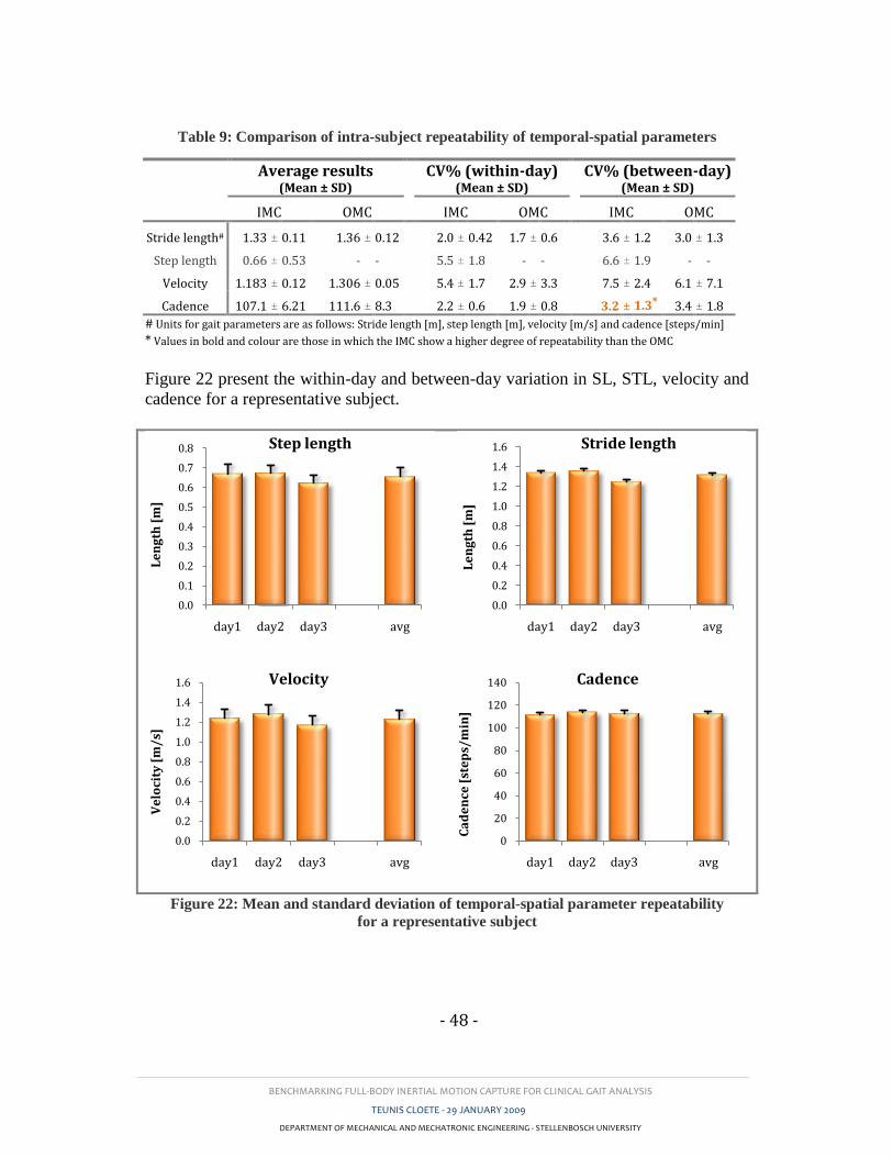
BENCHMARKING FULL-BODY INERTIAL MOTION CAPTURE FOR CLINICAL GAIT ANALYSIS
TEUNIS CLOETE - 29 JANUARY 2009
DEPARTMENT OF MECHANICAL AND MECHATRONIC ENGINEERING - STELLENBOSCH UNIVERSITY
- 48 -
Table 9: Comparison of intra-subject repeatability of temporal-spatial parameters
Figure 22 present the within-day and between-day variation in SL, STL, velocity and
cadence for a representative subject.
Figure 22: Mean and standard deviation of temporal-spatial parameter repeatability
for a representative subject
0.0
0.1
0.2
0.3
0.4
0.5
0.6
0.7
0.8
day1 day2 day3 avg
Le
ng
th [
m]
Step length
0.0
0.2
0.4
0.6
0.8
1.0
1.2
1.4
1.6
day1 day2 day3 avg
Le
ng
th [
m]
Stride length
0.0
0.2
0.4
0.6
0.8
1.0
1.2
1.4
1.6
day1 day2 day3 avg
Ve
loci
ty [
m/
s]
Velocity
0
20
40
60
80
100
120
140
day1 day2 day3 avg
Ca
de
nce
[st
ep
s/m
in]
Cadence
Average results
(Mean ± SD) CV% (within-day)
(Mean ± SD) CV% (between-day)
(Mean ± SD)
IMC OMC IMC OMC IMC OMC
Stride length# 1.33 ± 0.11 1.36 ± 0.12
2.0 ± 0.42 1.7 ± 0.6
3.6 ± 1.2 3.0 ± 1.3
Step length 0.66 ± 0.53 - -
5.5 ± 1.8 - -
6.6 ± 1.9 - -
Velocity 1.183 ± 0.12 1.306 ± 0.05
5.4 ± 1.7 2.9 ± 3.3
7.5 ± 2.4 6.1 ± 7.1
Cadence 107.1 ± 6.21 111.6 ± 8.3
2.2 ± 0.6 1.9 ± 0.8
3.2 ± 1.3* 3.4 ± 1.8
# Units for gait parameters are as follows: Stride length [m], step length [m], velocity [m/s] and cadence [steps/min]
* Values in bold and colour are those in which the IMC show a higher degree of repeatability than the OMC
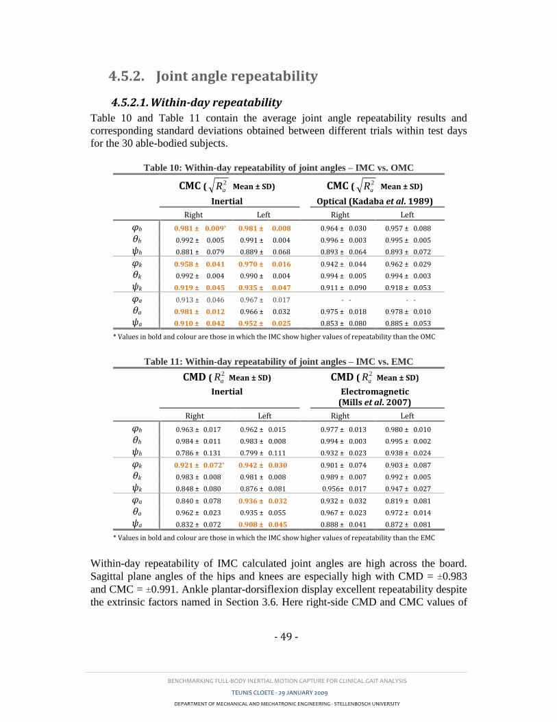
BENCHMARKING FULL-BODY INERTIAL MOTION CAPTURE FOR CLINICAL GAIT ANALYSIS
TEUNIS CLOETE - 29 JANUARY 2009
DEPARTMENT OF MECHANICAL AND MECHATRONIC ENGINEERING - STELLENBOSCH UNIVERSITY
- 49 -
4.5.2. Joint angle repeatability
4.5.2.1. Within-day repeatability
Table 10 and Table 11 contain the average joint angle repeatability results and
corresponding standard deviations obtained between different trials within test days
for the 30 able-bodied subjects.
Table 10: Within-day repeatability of joint angles – IMC vs. OMC
CMC ( 2
aR Mean ± SD)
Inertial
CMC ( 2
aR Mean ± SD)
Optical (Kadaba et al. 1989)
Right Left Right Left
φh 0.981 ± 0.009* 0.981 ± 0.008 0.964 ± 0.030 0.957 ± 0.088
θh 0.992 ± 0.005 0.991 ± 0.004 0.996 ± 0.003 0.995 ± 0.005
ψh 0.881 ± 0.079 0.889 ± 0.068 0.893 ± 0.064 0.893 ± 0.072
φk 0.958 ± 0.041 0.970 ± 0.016 0.942 ± 0.044 0.962 ± 0.029
θk 0.992 ± 0.004 0.990 ± 0.004 0.994 ± 0.005 0.994 ± 0.003
ψk 0.919 ± 0.045 0.935 ± 0.047 0.911 ± 0.090 0.918 ± 0.053
φa 0.913 ± 0.046 0.967 ± 0.017 - - - -
θa 0.981 ± 0.012 0.966 ± 0.032 0.975 ± 0.018 0.978 ± 0.010
ψa 0.910 ± 0.042 0.952 ± 0.025 0.853 ± 0.080 0.885 ± 0.053
* Values in bold and colour are those in which the IMC show higher values of repeatability than the OMC
Table 11: Within-day repeatability of joint angles – IMC vs. EMC
CMD ( 2
aR Mean ± SD)
Inertial
CMD ( 2
aR Mean ± SD)
Electromagnetic (Mills et al. 2007)
Right Left Right Left
φh 0.963 ± 0.017 0.962 ± 0.015 0.977 ± 0.013 0.980 ± 0.010
θh 0.984 ± 0.011 0.983 ± 0.008 0.994 ± 0.003 0.995 ± 0.002
ψh 0.786 ± 0.131 0.799 ± 0.111 0.932 ± 0.023 0.938 ± 0.024
φk 0.921 ± 0.072* 0.942 ± 0.030 0.901 ± 0.074 0.903 ± 0.087
θk 0.983 ± 0.008 0.981 ± 0.008 0.989 ± 0.007 0.992 ± 0.005
ψk 0.848 ± 0.080 0.876 ± 0.081 0.956± 0.017 0.947 ± 0.027
φa 0.840 ± 0.078 0.936 ± 0.032 0.932 ± 0.032 0.819 ± 0.081
θa 0.962 ± 0.023 0.935 ± 0.055 0.967 ± 0.023 0.972 ± 0.014
ψa 0.832 ± 0.072 0.908 ± 0.045 0.888 ± 0.041 0.872 ± 0.081
* Values in bold and colour are those in which the IMC show higher values of repeatability than the EMC
Within-day repeatability of IMC calculated joint angles are high across the board.
Sagittal plane angles of the hips and knees are especially high with CMD = ±0.983
and CMC = ±0.991. Ankle plantar-dorsiflexion display excellent repeatability despite
the extrinsic factors named in Section 3.6. Here right-side CMD and CMC values of
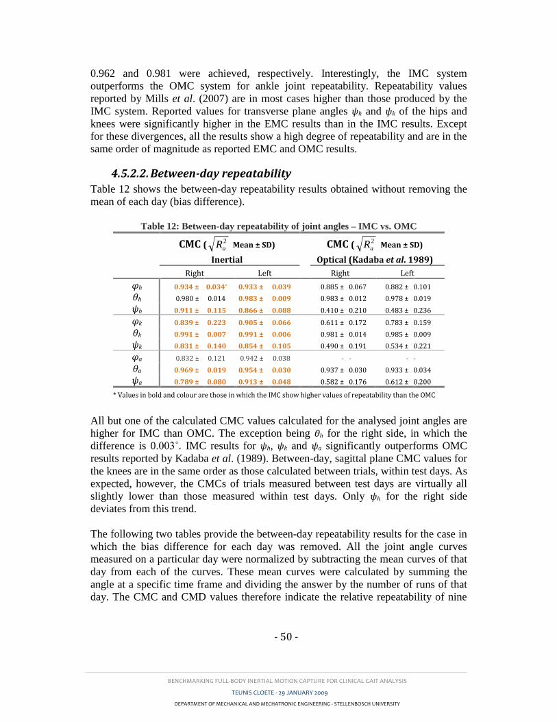
BENCHMARKING FULL-BODY INERTIAL MOTION CAPTURE FOR CLINICAL GAIT ANALYSIS
TEUNIS CLOETE - 29 JANUARY 2009
DEPARTMENT OF MECHANICAL AND MECHATRONIC ENGINEERING - STELLENBOSCH UNIVERSITY
- 50 -
0.962 and 0.981 were achieved, respectively. Interestingly, the IMC system
outperforms the OMC system for ankle joint repeatability. Repeatability values
reported by Mills et al. (2007) are in most cases higher than those produced by the
IMC system. Reported values for transverse plane angles ψh and ψk of the hips and
knees were significantly higher in the EMC results than in the IMC results. Except
for these divergences, all the results show a high degree of repeatability and are in the
same order of magnitude as reported EMC and OMC results.
4.5.2.2. Between-day repeatability
Table 12 shows the between-day repeatability results obtained without removing the
mean of each day (bias difference).
Table 12: Between-day repeatability of joint angles – IMC vs. OMC
CMC ( 2
aR Mean ± SD)
Inertial
CMC ( 2
aR Mean ± SD)
Optical (Kadaba et al. 1989)
Right Left Right Left
φh 0.934 ± 0.034* 0.933 ± 0.039 0.885 ± 0.067 0.882 ± 0.101
θh 0.980 ± 0.014 0.983 ± 0.009 0.983 ± 0.012 0.978 ± 0.019
ψh 0.911 ± 0.115 0.866 ± 0.088 0.410 ± 0.210 0.483 ± 0.236
φk 0.839 ± 0.223 0.905 ± 0.066 0.611 ± 0.172 0.783 ± 0.159
θk 0.991 ± 0.007 0.991 ± 0.006 0.981 ± 0.014 0.985 ± 0.009
ψk 0.831 ± 0.140 0.854 ± 0.105 0.490 ± 0.191 0.534 ± 0.221
φa 0.832 ± 0.121 0.942 ± 0.038 - - - -
θa 0.969 ± 0.019 0.954 ± 0.030 0.937 ± 0.030 0.933 ± 0.034
ψa 0.789 ± 0.080 0.913 ± 0.048 0.582 ± 0.176 0.612 ± 0.200
* Values in bold and colour are those in which the IMC show higher values of repeatability than the OMC
All but one of the calculated CMC values calculated for the analysed joint angles are
higher for IMC than OMC. The exception being θh for the right side, in which the
difference is 0.003˚. IMC results for ψh, ψk and ψa significantly outperforms OMC
results reported by Kadaba et al. (1989). Between-day, sagittal plane CMC values for
the knees are in the same order as those calculated between trials, within test days. As
expected, however, the CMCs of trials measured between test days are virtually all
slightly lower than those measured within test days. Only ψh for the right side
deviates from this trend.
The following two tables provide the between-day repeatability results for the case in
which the bias difference for each day was removed. All the joint angle curves
measured on a particular day were normalized by subtracting the mean curves of that
day from each of the curves. These mean curves were calculated by summing the
angle at a specific time frame and dividing the answer by the number of runs of that
day. The CMC and CMD values therefore indicate the relative repeatability of nine
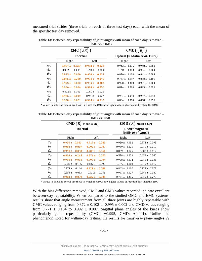
BENCHMARKING FULL-BODY INERTIAL MOTION CAPTURE FOR CLINICAL GAIT ANALYSIS
TEUNIS CLOETE - 29 JANUARY 2009
DEPARTMENT OF MECHANICAL AND MECHATRONIC ENGINEERING - STELLENBOSCH UNIVERSITY
- 51 -
measured trial strides (three trials on each of three test days) each with the mean of
the specific test day removed.
Table 13: Between-day repeatability of joint angles with mean of each day removed –
IMC vs. OMC
CMC ( 2
aR )
Inertial
CMC ( 2
aR )
Optical (Kadaba et al. 1989)
Right Left Right Left
φh 0.964 ± 0.028* 0.958 ± 0.023 0.943 ± 0.035 0.948 ± 0.062
θh 0.992 ± 0.003 0.991 ± 0.004 0.994± 0.003 0.994 ± 0.004
ψh 0.975 ± 0.020 0.950 ± 0.037 0.820 ± 0.100 0.841 ± 0.084
φk 0.875 ± 0.200 0.934 ± 0.040 0.737 ± 0.197 0.858 ± 0.106
θk 0.995 ± 0.002 0.995 ± 0.002 0.990 ± 0.009 0.991 ± 0.004
ψk 0.906 ± 0.084 0.910 ± 0.056 0.844 ± 0.086 0.849 ± 0.091
φa 0.872 ± 0.103 0.960 ± 0.025 - - - -
θa 0.976 ± 0.017 0.964± 0.027 0.964 ± 0.018 0.967 ± 0.013
ψa 0.950 ± 0.021 0.965 ± 0.015 0.834 ± 0.074 0.858 ± 0.055
* Values in bold and colour are those in which the IMC show higher values of repeatability than the OMC
Table 14: Between-day repeatability of joint angles with mean of each day removed –
IMC vs. EMC
CMD ( 2
aR Mean ± SD)
Inertial
CMD ( 2
aR Mean ± SD)
Electromagnetic (Mills et al. 2007)
Right Left Right Left
φh 0.930 ± 0.053* 0.919 ± 0.043 0.929 ± 0.052 0.871 ± 0.093
θh 0.984 ± 0.007 0.992 ± 0.007 0.969 ± 0.021 0.970 ± 0.019
ψh 0.951 ± 0.038 0.903 ± 0.068 0.839 ± 0.126 0.806 ± 0.112
φk 0.804 ± 0.265 0.874 ± 0.073 0.598 ± 0.220 0.659 ± 0.260
θk 0.991 ± 0.004 0.990 ± 0.004 0.988 ± 0.012 0.978 ± 0.036
ψk 0.827 ± 0.135 0.832 ± 0.099 0.877± 0.108 0.849 ± 0.112
φa 0.771 ± 0.164 0.921 ± 0.048 0.863 ± 0.102 0.722 ± 0.273
θa 0.953 ± 0.033 0.930± 0.051 0.967 ± 0.027 0.946 ± 0.080
ψa 0.903 ± 0.039 0.932 ± 0.029 0.731 ± 0.255 0.719 ± 0.273
* Values in bold and colour are those in which the IMC show higher values of repeatability than the EMC
With the bias difference removed, CMC and CMD values recorded indicate excellent
between-day repeatability. When compared to the studied OMC and EMC systems,
results show that angle measurement from all three joints are highly repeatable with
CMC values ranging from 0.872 ± 0.103 to 0.995 ± 0.002 and CMD values ranging
from 0.771 ± 0.164 to 0.992 ± 0.007. Sagittal plane angles of the knees show
particularly good repeatability (CMC: ±0.995, CMD: ±0.991). Unlike the
phenomenon noted for within-day testing, the results for transverse plane angles ψh
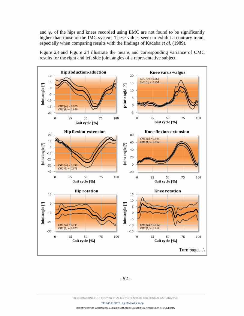
BENCHMARKING FULL-BODY INERTIAL MOTION CAPTURE FOR CLINICAL GAIT ANALYSIS
TEUNIS CLOETE - 29 JANUARY 2009
DEPARTMENT OF MECHANICAL AND MECHATRONIC ENGINEERING - STELLENBOSCH UNIVERSITY
- 52 -
and ψk of the hips and knees recorded using EMC are not found to be significantly
higher than those of the IMC system. These values seem to exhibit a contrary trend,
especially when comparing results with the findings of Kadaba et al. (1989).
Figure 23 and Figure 24 illustrate the means and corresponding variance of CMC
results for the right and left side joint angles of a representative subject.
Turn page…\
-20
-15
-10
-5
0
5
10
0 25 50 75 100
Join
t a
ng
le [
°]
Gait cycle [%]
Hip abduction-aduction
CMC (w) = 0.985CMC (b) = 0.959
-5
0
5
10
15
20
0 25 50 75 100
Join
t a
ng
le [
°]Gait cycle [%]
Knee varus-valgus
CMC (w) = 0.962CMC (b) = 0.951
-40
-30
-20
-10
0
10
20
0 25 50 75 100
Join
t a
ng
le [
°]
Gait cycle [%]
Hip flexion-extension
CMC (w) = 0.990CMC (b) = 0.973
-20
0
20
40
60
80
0 25 50 75 100
Join
t a
ng
le [
°]
Gait cycle [%]
Knee flexion-extension
CMC (w) = 0.989CMC (b) = 0.982
-30
-20
-10
0
10
0 25 50 75 100
Join
t a
ng
le [
°]
Gait cycle [%]
Hip rotation
CMC (w) = 0.944CMC (b) = 0.829
-15
-10
-5
0
5
10
15
0 25 50 75 100
Join
t a
ng
le [
°]
Gait cycle [%]
Knee rotation
CMC (w) = 0.902CMC (b) = 0.660

BENCHMARKING FULL-BODY INERTIAL MOTION CAPTURE FOR CLINICAL GAIT ANALYSIS
TEUNIS CLOETE - 29 JANUARY 2009
DEPARTMENT OF MECHANICAL AND MECHATRONIC ENGINEERING - STELLENBOSCH UNIVERSITY
- 53 -
Figure 23: Mean and variance of joint angle motion of the right side for the
representative subject over nine runs (three runs on each of the three days)
-15
-10
-5
0
5
0 25 50 75 100
Join
t a
ng
le [
°]
Gait cycle [%]
Ankle inversion-eversion
CMC (w) = 0.882CMC (b) = 0.730
-20
-10
0
10
20
30
0 25 50 75 100
Join
t a
ng
le [
°]
Gait cycle [%]
Ankle plantar-dorsiflexion
CMC (w) = 0.989CMC (b) = 0.982
-30
-20
-10
0
10
20
0 25 50 75 100
Join
t a
ng
le [
°]
Gait cycle [%]
Ankle rotation
CMC (w) = 0.952CMC (b) = 0.768
Average joint angle Variance over nine runs
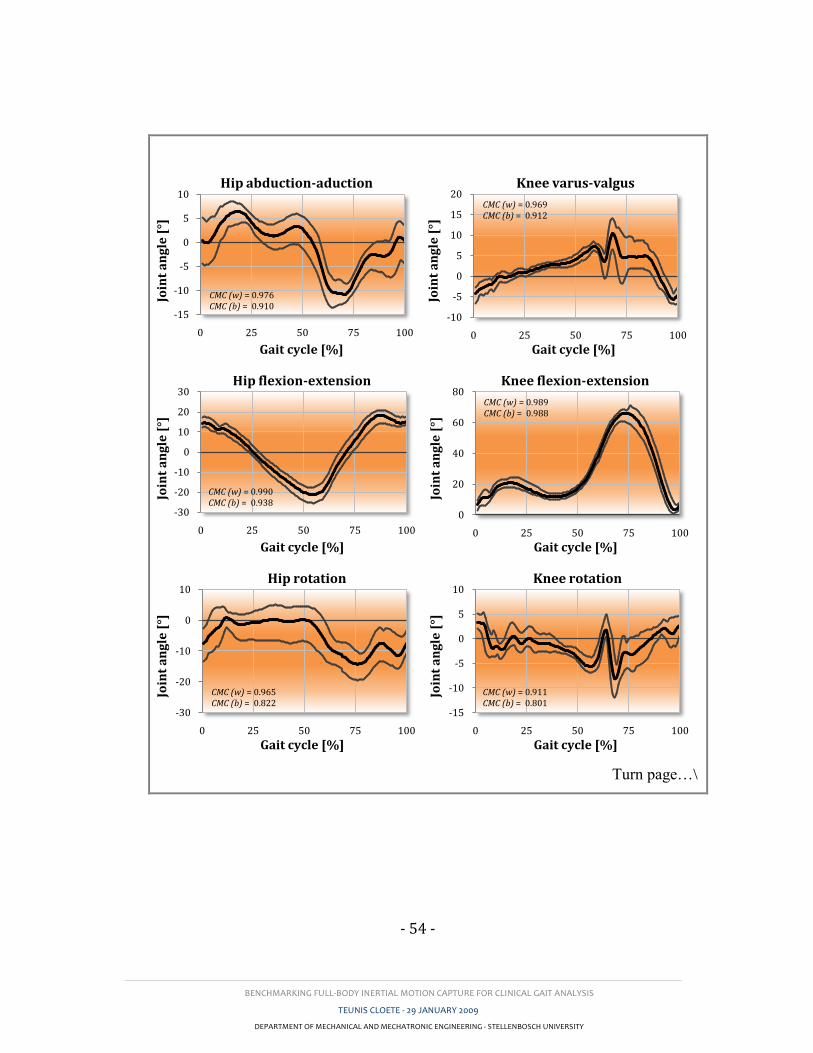
BENCHMARKING FULL-BODY INERTIAL MOTION CAPTURE FOR CLINICAL GAIT ANALYSIS
TEUNIS CLOETE - 29 JANUARY 2009
DEPARTMENT OF MECHANICAL AND MECHATRONIC ENGINEERING - STELLENBOSCH UNIVERSITY
- 54 -
Turn page…\
-15
-10
-5
0
5
10
0 25 50 75 100
Join
t a
ng
le [
°]
Gait cycle [%]
Hip abduction-aduction
CMC (w) = 0.976CMC (b) = 0.910
-10
-5
0
5
10
15
20
0 25 50 75 100
Join
t a
ng
le [
°]
Gait cycle [%]
Knee varus-valgus
CMC (w) = 0.969CMC (b) = 0.912
-30
-20
-10
0
10
20
30
0 25 50 75 100
Join
t a
ng
le [
°]
Gait cycle [%]
Hip flexion-extension
CMC (w) = 0.990CMC (b) = 0.938
0
20
40
60
80
0 25 50 75 100
Join
t a
ng
le [
°]
Gait cycle [%]
Knee flexion-extension
CMC (w) = 0.989CMC (b) = 0.988
-30
-20
-10
0
10
0 25 50 75 100
Join
t a
ng
le [
°]
Gait cycle [%]
Hip rotation
CMC (w) = 0.965CMC (b) = 0.822
-15
-10
-5
0
5
10
0 25 50 75 100
Join
t a
ng
le [
°]
Gait cycle [%]
Knee rotation
CMC (w) = 0.911CMC (b) = 0.801
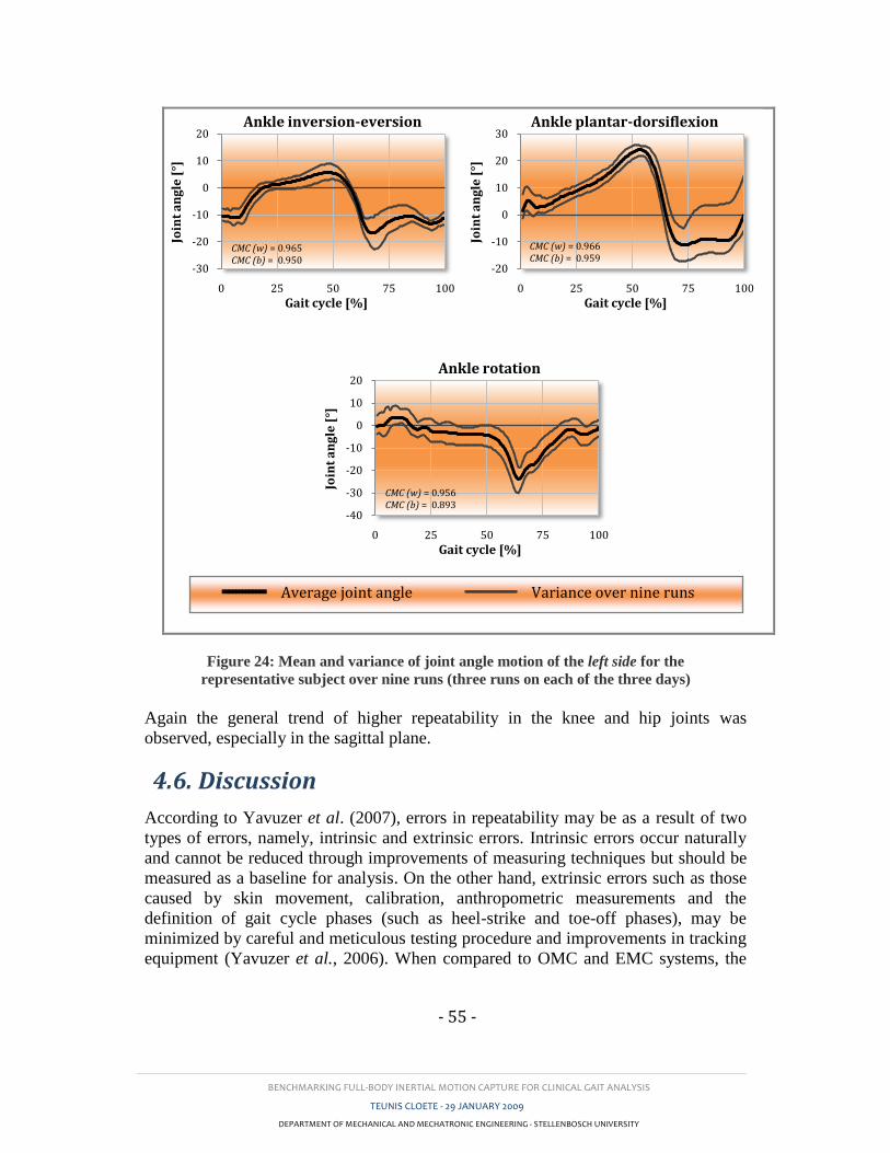
BENCHMARKING FULL-BODY INERTIAL MOTION CAPTURE FOR CLINICAL GAIT ANALYSIS
TEUNIS CLOETE - 29 JANUARY 2009
DEPARTMENT OF MECHANICAL AND MECHATRONIC ENGINEERING - STELLENBOSCH UNIVERSITY
- 55 -
Figure 24: Mean and variance of joint angle motion of the left side for the
representative subject over nine runs (three runs on each of the three days)
Again the general trend of higher repeatability in the knee and hip joints was
observed, especially in the sagittal plane.
4.6. Discussion
According to Yavuzer et al. (2007), errors in repeatability may be as a result of two
types of errors, namely, intrinsic and extrinsic errors. Intrinsic errors occur naturally
and cannot be reduced through improvements of measuring techniques but should be
measured as a baseline for analysis. On the other hand, extrinsic errors such as those
caused by skin movement, calibration, anthropometric measurements and the
definition of gait cycle phases (such as heel-strike and toe-off phases), may be
minimized by careful and meticulous testing procedure and improvements in tracking
equipment (Yavuzer et al., 2006). When compared to OMC and EMC systems, the
-30
-20
-10
0
10
20
0 25 50 75 100
Join
t a
ng
le [
°]
Gait cycle [%]
Ankle inversion-eversion
CMC (w) = 0.965CMC (b) = 0.950
-20
-10
0
10
20
30
0 25 50 75 100
Join
t a
ng
le [
°]
Gait cycle [%]
Ankle plantar-dorsiflexion
CMC (w) = 0.966CMC (b) = 0.959
-40
-30
-20
-10
0
10
20
0 25 50 75 100
Join
t a
ng
le [
°]
Gait cycle [%]
Ankle rotation
CMC (w) = 0.956CMC (b) = 0.893
Average joint angle Variance over nine runs
BENCHMARKING FULL-BODY INERTIAL MOTION CAPTURE FOR CLINICAL GAIT ANALYSIS
TEUNIS CLOETE - 29 JANUARY 2009
DEPARTMENT OF MECHANICAL AND MECHATRONIC ENGINEERING - STELLENBOSCH UNIVERSITY
- 56 -
IMC sensors are quite large (38 × 53 × 21 mm, 0.030 kg). This causes more sensor
inertia and subsequent increased skin artefacts, especially during faster ambulation.
On the other hand, a greater area of contact between the sensors and skin was
possible which ensured negligible sensor-to-skin movement. Heel-strike and toe-off
identification differences played a definite role, and further refinement of these
calculations is still required. Finally, calibration and anthropometric measurement
errors were minimized by using a single trained researcher to conduct segment
measurement and calibration for all the tests. Tester-tester effects were studied by
Besier et al. (2003) and Mills et al. (2007). Besier et al. concluded that the
repeatability results were fairly independent of the examiner.
Variation in marker reapplication also leads to an extrinsic bias error (Kadaba et al.,
1989). According to Mackey et al. (2005), small changes in marker positioning of
knee and ankle markers lead to noticeable differences in transverse plane kinematics.
This is consistent with findings by other researchers and apparent in the
comparatively lower between-day repeatability. In general however the between-day
repeatability results were high for both bias-uncorrected (CMC: 0.789 – 0.991) and
bias-corrected (CMC: 0.872 – 0.995) cases and comparable to those by Kadaba et al.
(1989) (CMC: 0.410 – 0.985 and 0.737 – 0.994) and Mills et al. (2005) (CMD: 0.598
– 0.988). This implies that marker reapplication errors were acceptably low.
Kadaba et al. (1989) stated that lower repeatability in the pelvic tilt was as a result of
both small range of motion (ROM) and the lack of a well defined pattern of
movement. This statement is true for most joint angles which display these
characteristics. Sagittal plane angles have higher ranges of motion and well defined
motion patterns (refer to Figure 23 and Figure 24). As expected these angles show the
highest CMCs. This is true for other studies (Kadaba et al., 1989, Mills et al., 2007).
Since the study conducted by Kadaba et al. (1989) OMC systems may have
improved, hence their reported values of repeatability may be slightly lower than
those achievable by present OMC systems, but to the knowledge of the author, no
such results have been reported.
Based on repeatability results obtained, this study has proven that researchers and/or
physicians can base diagnosis about the gait of a test subject or patient on a single
IMC-recorded gait analysis. Kadaba et al. (1989) however aptly stated that the
repeatability of pathological gait patient may decrease from those recorded from able-
bodied subjects, particularly because of greater skin looseness and a higher average
body-fat index often found in stroke and Parkinson’s disease sufferers.
BENCHMARKING FULL-BODY INERTIAL MOTION CAPTURE FOR CLINICAL GAIT ANALYSIS
TEUNIS CLOETE - 29 JANUARY 2009
DEPARTMENT OF MECHANICAL AND MECHATRONIC ENGINEERING - STELLENBOSCH UNIVERSITY
- 57 -
5. NEURAL NETWORK
5.1. Introduction
The aim, in earlier sections, was to show that IMC (more specifically full-body IMC)
exhibits sufficient accuracy and repeatability to be utilized for clinical gait analysis.
The results obtained in Sections 3 and 4 indicate that this is indeed the case. This
section aims to compliment these findings by employing and evaluating IMC in a
clinical application namely to train and test a neural network using IMC collected
data, to distinguish between stroke patients and able-bodied controls. Although a
seemingly trivial problem, human gait is observed to be very complex and variable,
even within an able-bodied group. Subjects from one group may display
characteristics common to the other group.
The use of semi-automated-diagnosis tools such as neural networks has seen a
continual growth in popularity because of their clinical potential and diagnostic
success. As will be shown in later sections, it is often very difficult to provide
accurate diagnoses by looking at only a few parameters at a time. However, a neural
network is able to perform a weighted comparison of several input parameters
simultaneously to distinguish between known output groups. This aids medical
professionals with patient assessment by supplying a primary diagnosis, which may
provide both an increase in the number of patients that a doctor is able to treat as well
as improve the choice and quality of treatment.
5.2. Objectives
In this section the author aims to prove, through the use a neural network in a specific
clinical application, the usefulness of employing a neural network for gait analysis
over the use of conventional qualitative or quantitative statistical methods. This
section also aims to highlight the present and future advantages of combining IMC
and semi-automated-diagnosis tools (e.g. neural networks or fuzzy logic) in gait
analysis. Such advantages may be especially useful in telemedicine.
5.3. Procedure
5.3.1. Data collection
5.3.1.1. Inclusion criteria
Sufficient pathologic and normal gait data was required to train and test a chosen
neural network. Data from the 30 able-bodied subjects used in the repeatability study
(Section 4) was re-used for the required normal input data. Stroke patient data was
recorded in a collaborative study done in cooperation with Mr Wasim Labban from
BENCHMARKING FULL-BODY INERTIAL MOTION CAPTURE FOR CLINICAL GAIT ANALYSIS
TEUNIS CLOETE - 29 JANUARY 2009
DEPARTMENT OF MECHANICAL AND MECHATRONIC ENGINEERING - STELLENBOSCH UNIVERSITY
- 58 -
the Department of Physiotherapy of the University of Stellenbosch. Ethical approval
for this study was obtained from the Committee for Human Research of the
University of Stellenbosch, Faculty of Life Sciences. Written informed consent was
obtained from each patient prior to their participation in the study. Routine gait
analysis was conducted on 28 hemiparetic stroke patients with varying degrees of
locomotive dysfunction. The stoke-patient group were aged between 25 and 64 years
with a mean (STD) of 51.2 (±10.1) compared to the control group who were aged
between 19 and 25 with a mean of 22.6 (±1.9). Also, the stroke-patient group
contained 40 % female subjects compared to the control group who were exclusively
male.
5.3.1.2. Gait assessment
Tests were conducted with the aid of Mr Labban at the Western Cape Rehabilitation
Centre. All test subjects were asked to walk at a self-selected speed along a 10 m
walkway. Measurements were recorded in one direction only. Stroke patients were
given sufficient opportunity to rest between trials. This minimized the effect of
fatigue on gait recordings. At least five trials, each with at least four full strides, were
recorded for each subject. 375 strides3 from 25 of the able-bodied subjects and 327
strides3 from 22 of the stroke patients were isolated as train data and 73 strides
3 from
the remaining five able-bodied subjects and 66 strides3 from the remaining five stroke
patients were used as test data for the neural network. All strides were re-sampled to
100 data points which represent 100% of the gait cycle.
5.3.2. Network input parameters
This section deals with the selection of input parameters with which the neural
network was trained. The first step was to calculate the Statistical Overlap Factor
(SOF) as proposed by Mdlanzi et al. (2007). The SOF between two variable
distributions is a calculation of the ratio of the distance between the averages of the
two distributions, to the mean of the two standard deviations. This is represented by
Equation (16) below:
2/)( 21
21 xxSOF
(16)
where 1x and 2x are the averages of the distributions and 1 and 2 are their
respective standard deviations (Mdlanzi et al., 2007).
High SOF values indicate a greater degree of separation between the respective
distributions. This is indicated in Figure 25 which shows the stroke-patient and able-
bodied control group distributions for the input parameters having the ten highest
calculated SOF values.
3 In this context, the term “strides”, refers to a combination of concurrent left and right-side strides.
This was necessary to calculate parameters such as SL and double-stance and swing phases.
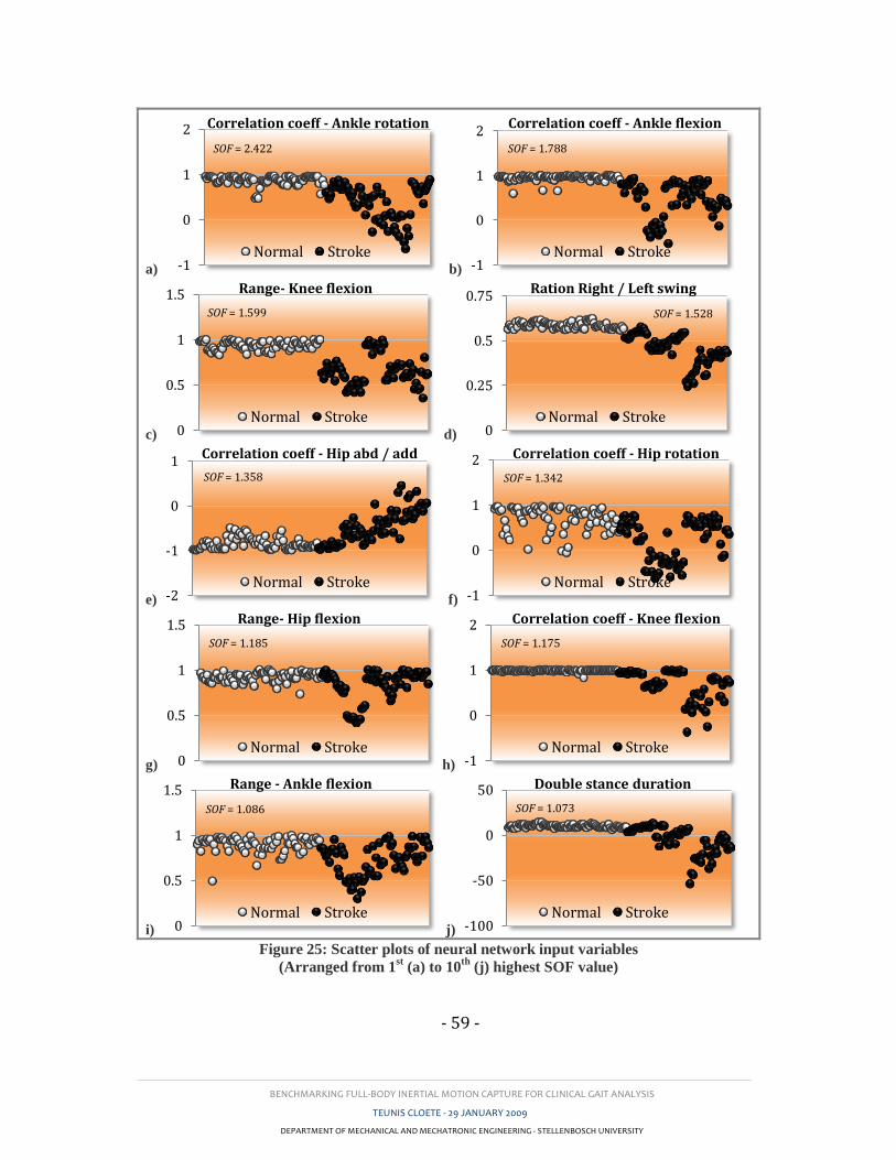
BENCHMARKING FULL-BODY INERTIAL MOTION CAPTURE FOR CLINICAL GAIT ANALYSIS
TEUNIS CLOETE - 29 JANUARY 2009
DEPARTMENT OF MECHANICAL AND MECHATRONIC ENGINEERING - STELLENBOSCH UNIVERSITY
- 59 -
a) b)
c) d)
e) f)
g) h)
i) j)
Figure 25: Scatter plots of neural network input variables
(Arranged from 1st (a) to 10
th (j) highest SOF value)
-1
0
1
2 Correlation coeff - Ankle rotation
Normal Stroke
SOF = 2.422
-1
0
1
2Correlation coeff - Ankle flexion
Normal Stroke
SOF = 1.788
0
0.5
1
1.5 Range- Knee flexion
Normal Stroke
SOF = 1.599
0
0.25
0.5
0.75Ration Right / Left swing
Normal Stroke
SOF = 1.528
-2
-1
0
1Correlation coeff - Hip abd / add
Normal Stroke
SOF = 1.358
-1
0
1
2 Correlation coeff - Hip rotation
Normal Stroke
SOF = 1.342
0
0.5
1
1.5 Range- Hip flexion
Normal Stroke
SOF = 1.185
-1
0
1
2 Correlation coeff - Knee flexion
Normal Stroke
SOF = 1.175
0
0.5
1
1.5 Range - Ankle flexion
Normal Stroke
SOF = 1.086
-100
-50
0
50 Double stance duration
Normal Stroke
SOF = 1.073
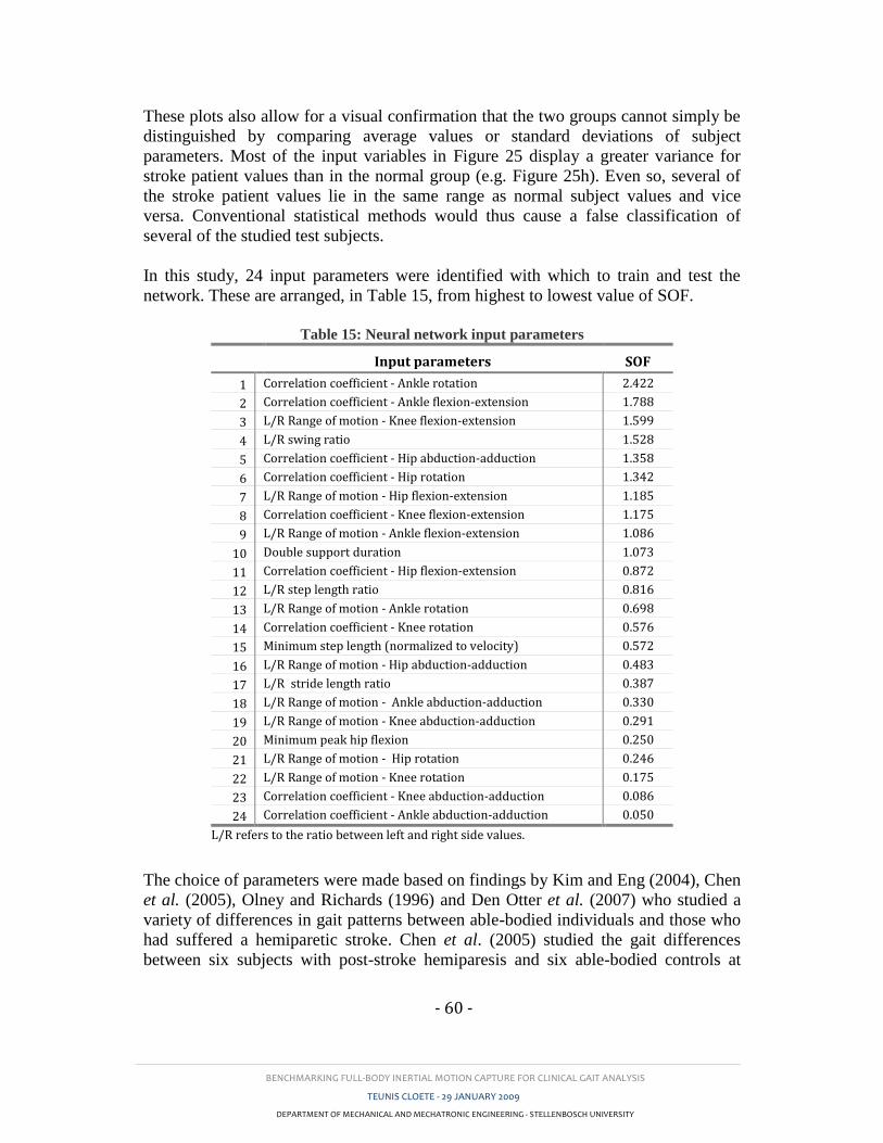
BENCHMARKING FULL-BODY INERTIAL MOTION CAPTURE FOR CLINICAL GAIT ANALYSIS
TEUNIS CLOETE - 29 JANUARY 2009
DEPARTMENT OF MECHANICAL AND MECHATRONIC ENGINEERING - STELLENBOSCH UNIVERSITY
- 60 -
These plots also allow for a visual confirmation that the two groups cannot simply be
distinguished by comparing average values or standard deviations of subject
parameters. Most of the input variables in Figure 25 display a greater variance for
stroke patient values than in the normal group (e.g. Figure 25h). Even so, several of
the stroke patient values lie in the same range as normal subject values and vice
versa. Conventional statistical methods would thus cause a false classification of
several of the studied test subjects.
In this study, 24 input parameters were identified with which to train and test the
network. These are arranged, in Table 15, from highest to lowest value of SOF.
Table 15: Neural network input parameters
Input parameters SOF
1
2
3
4
5
6
7
8
9
10
11
12
13
14
15
16
17
18
19
20
21
22
23
24
Correlation coefficient - Ankle rotation
Correlation coefficient - Ankle flexion-extension
L/R Range of motion - Knee flexion-extension
L/R swing ratio
Correlation coefficient - Hip abduction-adduction
Correlation coefficient - Hip rotation
L/R Range of motion - Hip flexion-extension
Correlation coefficient - Knee flexion-extension
L/R Range of motion - Ankle flexion-extension
Double support duration
Correlation coefficient - Hip flexion-extension
L/R step length ratio
L/R Range of motion - Ankle rotation
Correlation coefficient - Knee rotation
Minimum step length (normalized to velocity)
L/R Range of motion - Hip abduction-adduction
L/R stride length ratio
L/R Range of motion - Ankle abduction-adduction
L/R Range of motion - Knee abduction-adduction
Minimum peak hip flexion
L/R Range of motion - Hip rotation
L/R Range of motion - Knee rotation
Correlation coefficient - Knee abduction-adduction
Correlation coefficient - Ankle abduction-adduction
2.422
1.788
1.599
1.528
1.358
1.342
1.185
1.175
1.086
1.073
0.872
0.816
0.698
0.576
0.572
0.483
0.387
0.330
0.291
0.250
0.246
0.175
0.086
0.050
L/R refers to the ratio between left and right side values.
The choice of parameters were made based on findings by Kim and Eng (2004), Chen
et al. (2005), Olney and Richards (1996) and Den Otter et al. (2007) who studied a
variety of differences in gait patterns between able-bodied individuals and those who
had suffered a hemiparetic stroke. Chen et al. (2005) studied the gait differences
between six subjects with post-stroke hemiparesis and six able-bodied controls at
BENCHMARKING FULL-BODY INERTIAL MOTION CAPTURE FOR CLINICAL GAIT ANALYSIS
TEUNIS CLOETE - 29 JANUARY 2009
DEPARTMENT OF MECHANICAL AND MECHATRONIC ENGINEERING - STELLENBOSCH UNIVERSITY
- 61 -
matched speeds and found a noticeable distinction between swing-time and step-
length asymmetry of the left and right sides. Asymmetry of swing-time in post-stroke
subjects was found to be more than 40% higher than the average value calculated for
the able-bodied group (Chen et al., 2005). Otter et al. (2007) analysed temporal gait
in 24 hemiparetic stroke patients and 14 able-bodied controls and found significant
differences in double-stance and single-stance values. Olney and Richards (1996)
stated that only 23 - 37% of persons having suffered hemiparetic stroke are able to
walk independently within the first week. This value increases to between 50 - 80%
after 3 weeks.
Notice that the asymmetry between the left and right side ankle joint angles in the
transverse and sagittal planes produce the highest values of SOF. The asymmetry was
calculated by taking the correlation coefficient of the left and right side joint-angle
curves. Other input parameters include: the ratio between the left and right side
maximum range of motion (ROM) for all nine joint angles, the ratio of left and right
swing phase to gait cycle, the double-support duration, the minimum step length, the
minimum peak hip flexion-extension and the ratio of left to right step and stride
lengths. The ROM was calculated from the displacement between the minimum and
maximum joint angles measured during a single gait cycle for a specific side. The
ratio of left to right side ROMs were then taken as input parameters. The term L/R in
Table 15 refers to the ratio between the left and right side values. However, since
different stroke patients exhibit hemiparesis in different sides of the body, the ratio of
L/R was corrected to represent the ratio of the lower of the two values to the higher.
These values are therefore always equal to, or lower than one, where a value of one
implies perfect symmetry between the left and right sides. Figure 25 clearly illustrates
this feature. The swing phase for a specific side is the time period between the toe-off
instance and the following heel-strike instance. This parameter was chosen because
stroke patients tend to display a shorter swing phase in their unaffected side than on
their affected side. Similarly stroke patients tend to exhibit a prolonged double-
support to aid in their stability. The double-support phase is calculated as the period
between the heel-strike instance of one side and the toe-off instance of the other side.
During this phase both feet are in contact with the ground.
Stroke patients have a tendency to walk at a lower average velocity than able-bodied
subjects. Although this attribute is significant and fairly consistent, a possibility is
there that an able-bodied subject walks at a slow speed or that a stroke patient walks
at a near normal speed. It was therefore decided to eliminate the effect of velocity by
normalizing the step length and evaluating the minimum normalized step length.
Stroke patients demonstrate a significantly reduced hip extension. To compensate for
this they often exhibit a decrease in hip flexion on the affected side. This
characteristic was employed by comparing the minimum peak hip flexion of the two
sides. Finally the asymmetries of the step and stride lengths were assessed by taking
the ratio between the left and right side lengths.
BENCHMARKING FULL-BODY INERTIAL MOTION CAPTURE FOR CLINICAL GAIT ANALYSIS
TEUNIS CLOETE - 29 JANUARY 2009
DEPARTMENT OF MECHANICAL AND MECHATRONIC ENGINEERING - STELLENBOSCH UNIVERSITY
- 62 -
5.3.3. Training and testing the model
Neural network training and testing parameter matrices were prepared as instructed
by the MATLAB2007b neural network toolbox. To achieve the best possible
diagnostic performance, network variables such as the goal function (tolerance), the
number of hidden-layer neurons and the number of input parameters were optimized.
This was accomplished by varying these values within pilot-test-determined ranges
and comparing the number of misclassified strides. The goal function was varied
between 0.025 and 0.2 in increments of 0.025. The number of input parameters was
incrementally decreased from 24 to 4. The parameter with the lowest SOF value was
eliminated after each iteration. A rule-of-thumb is that the number of hidden-layer
neurons be twice the number of input parameters. This was taken as a reference point
around which the number of neurons was varied from seven less to seven more than
this point. This is illustrated in the tables shown in Section 5.4.
It was found that the network was unstable at certain combinations of these
parameters. It was therefore necessary to test the repeatability of the network at
different input scenarios. This was achieved by running the same optimization
procedure, mentioned above, 15 times. By doing so, the mean and standard deviation
of each scenario could be evaluated over 15 identical runs in order to find the
optimum combination of neural network input variables. Optimization results are
shown in Section 5.4.
5.3.4. Network training function selection
The MATLAB 2007b neural network toolbox contains several network training
functions to choose from. To select the most apt of these functions for the gait data
used, three functions were tested using the optimization technique described above.
Results were then tabulated as shown in Appendix E. This section will provide a
short description of each of the tested training functions followed by a discussion of
the selection process used to identify the most apt function for gait data:
5.3.4.1. TRAINLM
The network training function, trainlm.m, uses Levenberg-Marquardt
optimization to update weight and bias values. This function can train any network
provided its net input, weight, and transfer functions have derivative functions.
According to the MATLAB Help-menu, this train function assumes that the network
has the mse performance function which is a basic assumption of the Levenberg-
Marquardt algorithm.
The Jacobian (jX) of performance (perf) is calculated using back-propagation with
respect to the weight and bias variables (X) and each variable is adjusted according to
the Levenberg-Marquardt optimization as shown below:
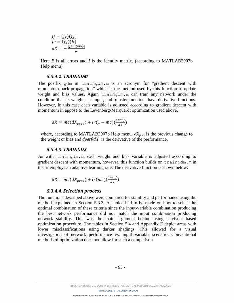
BENCHMARKING FULL-BODY INERTIAL MOTION CAPTURE FOR CLINICAL GAIT ANALYSIS
TEUNIS CLOETE - 29 JANUARY 2009
DEPARTMENT OF MECHANICAL AND MECHATRONIC ENGINEERING - STELLENBOSCH UNIVERSITY
- 63 -
Here E is all errors and I is the identity matrix. (according to MATLAB2007b
Help menu)
5.3.4.2. TRAINGDM
The postfix gdm in traingdm.m is an acronym for “gradient descent with
momentum back-propagation” which is the method used by this function to update
weight and bias values. Again traingdm.m can train any network under the
condition that its weight, net input, and transfer functions have derivative functions.
However, in this case each variable is adjusted according to gradient descent with
momentum in appose to the Levenberg-Marquardt optimization used above.
where, according to MATLAB2007b Help menu, dXprev is the previous change to
the weight or bias and dperf/dX is the derivative of the performance.
5.3.4.3. TRAINGDX
As with traingdm.m, each weight and bias variable is adjusted according to
gradient descent with momentum, however, this function builds on traingdm.m in
that it employs an adaptive learning rate. The derivative function is shown below:
5.3.4.4. Selection process
The functions described above were compared for stability and performance using the
method explained in Section 5.3.3. A choice had to be made on how to select the
optimal combination of these criteria since the input-variable combination producing
the best network performance did not match the input combination producing
network stability. This was the main argument behind using a visual based
optimization procedure. The tables in Section 5.4 and Appendix E depict areas with
lower misclassifications using darker shadings. This allowed for a visual
investigation of network performance vs. input variable scenario. Conventional
methods of optimization does not allow for such a comparison.
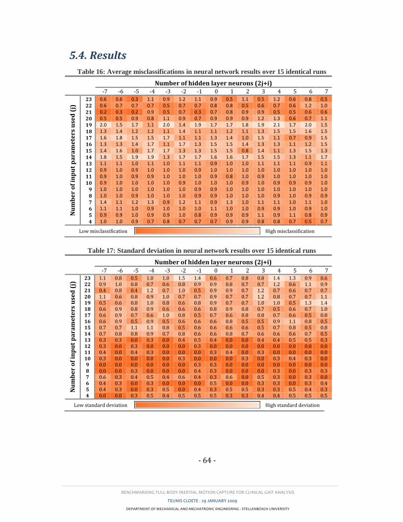
BENCHMARKING FULL-BODY INERTIAL MOTION CAPTURE FOR CLINICAL GAIT ANALYSIS
TEUNIS CLOETE - 29 JANUARY 2009
DEPARTMENT OF MECHANICAL AND MECHATRONIC ENGINEERING - STELLENBOSCH UNIVERSITY
- 64 -
5.4. Results
Table 16: Average misclassifications in neural network results over 15 identical runs
Number of hidden layer neurons (2j+i)
-7 -6 -5 -4 -3 -2 -1 0 1 2 3 4 5 6 7
Nu
mb
er
of
inp
ut
pa
ram
ete
rs u
sed
(j)
23 0.6 0.6 0.3 1.1 0.9 1.2 1.1 0.9 0.5 1.1 0.5 1.2 0.6 0.8 0.5
22 0.6 0.7 0.7 0.7 0.5 0.7 0.7 0.8 0.8 0.5 0.6 0.7 0.6 1.2 1.0
21 0.2 0.3 0.2 0.9 0.5 0.7 0.3 0.7 0.8 0.9 0.9 0.5 0.5 0.6 0.6
20 0.5 0.5 0.9 0.8 1.1 0.9 0.7 0.9 0.9 0.9 1.2 1.3 0.6 0.7 1.1
19 2.0 1.5 1.7 1.1 2.0 1.4 1.9 1.7 1.7 1.8 1.9 2.1 1.7 2.0 1.5
18 1.3 1.4 1.2 1.2 1.1 1.4 1.1 1.1 1.2 1.1 1.3 1.5 1.5 1.6 1.5
17 1.6 1.8 1.5 1.5 1.7 1.1 1.1 1.3 1.4 1.0 1.5 1.1 0.7 0.9 1.5
16 1.3 1.3 1.4 1.7 1.1 1.7 1.3 1.5 1.5 1.4 1.3 1.3 1.1 1.2 1.5
15 1.4 1.6 1.0 1.7 1.7 1.3 1.3 1.5 1.5 0.8 1.4 1.1 1.3 1.5 1.3
14 1.8 1.5 1.9 1.9 1.3 1.7 1.7 1.6 1.6 1.7 1.5 1.5 1.3 1.1 1.7
13 1.1 1.1 1.0 1.1 1.0 1.1 1.1 0.9 1.0 1.0 1.1 1.1 1.1 0.9 1.1
12 0.9 1.0 0.9 1.0 1.0 1.0 0.9 1.0 1.0 1.0 1.0 1.0 1.0 1.0 1.0
11 0.9 1.0 0.9 0.9 1.0 1.0 1.0 0.9 0.8 1.0 0.9 1.0 1.0 1.0 1.0
10 0.9 1.0 1.0 1.0 1.0 0.9 1.0 1.0 1.0 0.9 1.0 0.9 0.9 0.9 1.0
9 1.0 1.0 1.0 1.0 1.0 1.0 0.9 0.9 1.0 1.0 1.0 1.0 1.0 1.0 1.0
8 1.0 1.0 0.9 1.0 1.0 1.0 0.9 0.9 1.0 1.0 1.0 0.9 1.0 0.9 0.9
7 1.4 1.1 1.2 1.3 0.9 1.2 1.1 0.9 1.3 1.0 1.1 1.1 1.0 1.1 1.0
6 1.1 1.1 1.0 0.9 1.0 1.0 1.0 1.1 1.0 1.0 0.9 0.9 1.0 0.9 1.0
5 0.9 0.9 1.0 0.9 0.9 1.0 0.8 0.9 0.9 0.9 1.1 0.9 1.1 0.8 0.9
4 1.0 1.0 0.9 0.7 0.8 0.7 0.7 0.7 0.9 0.9 0.8 0.8 0.7 0.5 0.7
Low misclassification High misclassification
Table 17: Standard deviation in neural network results over 15 identical runs
Number of hidden layer neurons (2j+i)
-7 -6 -5 -4 -3 -2 -1 0 1 2 3 4 5 6 7
Nu
mb
er
of
inp
ut
pa
ram
ete
rs u
sed
(j)
23 1.1 0.8 0.5 1.0 1.0 1.5 1.4 0.6 0.7 0.8 0.8 1.4 1.3 0.9 0.6 22 0.9 1.0 0.8 0.7 0.6 0.8 0.9 0.9 0.8 0.7 0.7 1.2 0.6 1.1 0.9 21 0.4 0.8 0.4 1.2 0.7 1.0 0.5 0.9 0.9 0.7 1.2 0.7 0.6 0.7 0.7 20 1.1 0.6 0.8 0.9 1.0 0.7 0.7 0.9 0.7 0.7 1.2 0.8 0.7 0.7 1.1 19 0.5 0.6 0.8 1.0 0.8 0.6 0.8 0.9 0.7 0.7 1.0 1.0 0.5 1.3 1.4 18 0.6 0.9 0.8 0.9 0.6 0.6 0.6 0.8 0.9 0.8 0.7 0.5 0.6 0.7 1.0 17 0.6 0.9 0.7 0.6 1.0 0.8 0.5 0.7 0.6 0.8 0.8 0.7 0.6 0.5 0.8 16 0.6 0.9 0.5 0.9 0.5 0.6 0.6 0.6 0.8 0.5 0.5 0.9 1.1 0.8 0.5 15 0.7 0.7 1.1 1.1 0.8 0.5 0.6 0.6 0.6 0.6 0.5 0.7 0.8 0.5 0.8 14 0.7 0.8 0.8 0.9 0.7 0.8 0.6 0.6 0.8 0.7 0.6 0.6 0.6 0.7 0.5 13 0.3 0.3 0.0 0.3 0.0 0.4 0.5 0.4 0.0 0.0 0.4 0.4 0.5 0.5 0.3 12 0.3 0.0 0.3 0.0 0.0 0.0 0.3 0.0 0.0 0.0 0.0 0.0 0.0 0.0 0.0 11 0.4 0.0 0.4 0.3 0.0 0.0 0.0 0.3 0.4 0.0 0.3 0.0 0.0 0.0 0.0 10 0.3 0.0 0.0 0.0 0.0 0.3 0.0 0.0 0.0 0.3 0.0 0.3 0.4 0.3 0.0 9 0.0 0.0 0.0 0.0 0.0 0.0 0.3 0.3 0.0 0.0 0.0 0.0 0.0 0.0 0.0 8 0.0 0.0 0.3 0.0 0.0 0.0 0.4 0.3 0.0 0.0 0.0 0.3 0.0 0.3 0.3 7 0.6 0.3 0.4 0.5 0.4 0.6 0.4 0.3 0.6 0.0 0.5 0.3 0.0 0.3 0.0 6 0.4 0.3 0.0 0.3 0.0 0.0 0.0 0.5 0.0 0.0 0.3 0.3 0.0 0.3 0.4 5 0.4 0.3 0.0 0.3 0.5 0.0 0.4 0.3 0.5 0.5 0.3 0.3 0.5 0.4 0.3 4 0.0 0.0 0.3 0.5 0.4 0.5 0.5 0.5 0.3 0.3 0.4 0.4 0.5 0.5 0.5
Low standard deviation High standard deviation
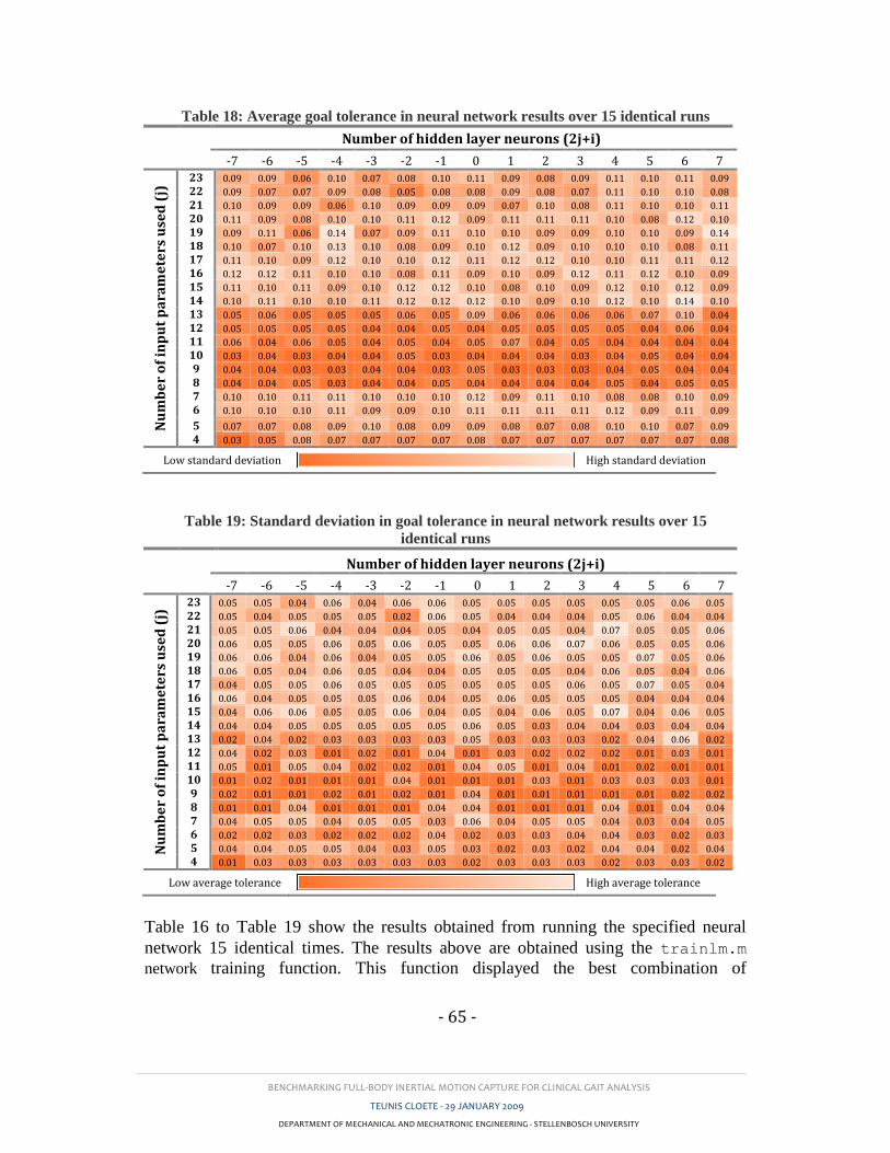
BENCHMARKING FULL-BODY INERTIAL MOTION CAPTURE FOR CLINICAL GAIT ANALYSIS
TEUNIS CLOETE - 29 JANUARY 2009
DEPARTMENT OF MECHANICAL AND MECHATRONIC ENGINEERING - STELLENBOSCH UNIVERSITY
- 65 -
Table 18: Average goal tolerance in neural network results over 15 identical runs
Number of hidden layer neurons (2j+i)
-7 -6 -5 -4 -3 -2 -1 0 1 2 3 4 5 6 7
Nu
mb
er
of
inp
ut
pa
ram
ete
rs u
sed
(j)
23 0.09 0.09 0.06 0.10 0.07 0.08 0.10 0.11 0.09 0.08 0.09 0.11 0.10 0.11 0.09
22 0.09 0.07 0.07 0.09 0.08 0.05 0.08 0.08 0.09 0.08 0.07 0.11 0.10 0.10 0.08
21 0.10 0.09 0.09 0.06 0.10 0.09 0.09 0.09 0.07 0.10 0.08 0.11 0.10 0.10 0.11
20 0.11 0.09 0.08 0.10 0.10 0.11 0.12 0.09 0.11 0.11 0.11 0.10 0.08 0.12 0.10
19 0.09 0.11 0.06 0.14 0.07 0.09 0.11 0.10 0.10 0.09 0.09 0.10 0.10 0.09 0.14
18 0.10 0.07 0.10 0.13 0.10 0.08 0.09 0.10 0.12 0.09 0.10 0.10 0.10 0.08 0.11
17 0.11 0.10 0.09 0.12 0.10 0.10 0.12 0.11 0.12 0.12 0.10 0.10 0.11 0.11 0.12
16 0.12 0.12 0.11 0.10 0.10 0.08 0.11 0.09 0.10 0.09 0.12 0.11 0.12 0.10 0.09
15 0.11 0.10 0.11 0.09 0.10 0.12 0.12 0.10 0.08 0.10 0.09 0.12 0.10 0.12 0.09
14 0.10 0.11 0.10 0.10 0.11 0.12 0.12 0.12 0.10 0.09 0.10 0.12 0.10 0.14 0.10
13 0.05 0.06 0.05 0.05 0.05 0.06 0.05 0.09 0.06 0.06 0.06 0.06 0.07 0.10 0.04
12 0.05 0.05 0.05 0.05 0.04 0.04 0.05 0.04 0.05 0.05 0.05 0.05 0.04 0.06 0.04
11 0.06 0.04 0.06 0.05 0.04 0.05 0.04 0.05 0.07 0.04 0.05 0.04 0.04 0.04 0.04
10 0.03 0.04 0.03 0.04 0.04 0.05 0.03 0.04 0.04 0.04 0.03 0.04 0.05 0.04 0.04
9 0.04 0.04 0.03 0.03 0.04 0.04 0.03 0.05 0.03 0.03 0.03 0.04 0.05 0.04 0.04
8 0.04 0.04 0.05 0.03 0.04 0.04 0.05 0.04 0.04 0.04 0.04 0.05 0.04 0.05 0.05
7 0.10 0.10 0.11 0.11 0.10 0.10 0.10 0.12 0.09 0.11 0.10 0.08 0.08 0.10 0.09
6 0.10 0.10 0.10 0.11 0.09 0.09 0.10 0.11 0.11 0.11 0.11 0.12 0.09 0.11 0.09
5 0.07 0.07 0.08 0.09 0.10 0.08 0.09 0.09 0.08 0.07 0.08 0.10 0.10 0.07 0.09
4 0.03 0.05 0.08 0.07 0.07 0.07 0.07 0.08 0.07 0.07 0.07 0.07 0.07 0.07 0.08
Low standard deviation High standard deviation
Table 19: Standard deviation in goal tolerance in neural network results over 15
identical runs
Number of hidden layer neurons (2j+i)
-7 -6 -5 -4 -3 -2 -1 0 1 2 3 4 5 6 7
Nu
mb
er
of
inp
ut
pa
ram
ete
rs u
sed
(j)
23 0.05 0.05 0.04 0.06 0.04 0.06 0.06 0.05 0.05 0.05 0.05 0.05 0.05 0.06 0.05
22 0.05 0.04 0.05 0.05 0.05 0.02 0.06 0.05 0.04 0.04 0.04 0.05 0.06 0.04 0.04
21 0.05 0.05 0.06 0.04 0.04 0.04 0.05 0.04 0.05 0.05 0.04 0.07 0.05 0.05 0.06
20 0.06 0.05 0.05 0.06 0.05 0.06 0.05 0.05 0.06 0.06 0.07 0.06 0.05 0.05 0.06
19 0.06 0.06 0.04 0.06 0.04 0.05 0.05 0.06 0.05 0.06 0.05 0.05 0.07 0.05 0.06
18 0.06 0.05 0.04 0.06 0.05 0.04 0.04 0.05 0.05 0.05 0.04 0.06 0.05 0.04 0.06
17 0.04 0.05 0.05 0.06 0.05 0.05 0.05 0.05 0.05 0.05 0.06 0.05 0.07 0.05 0.04
16 0.06 0.04 0.05 0.05 0.05 0.06 0.04 0.05 0.06 0.05 0.05 0.05 0.04 0.04 0.04
15 0.04 0.06 0.06 0.05 0.05 0.06 0.04 0.05 0.04 0.06 0.05 0.07 0.04 0.06 0.05
14 0.04 0.04 0.05 0.05 0.05 0.05 0.05 0.06 0.05 0.03 0.04 0.04 0.03 0.04 0.04
13 0.02 0.04 0.02 0.03 0.03 0.03 0.03 0.05 0.03 0.03 0.03 0.02 0.04 0.06 0.02
12 0.04 0.02 0.03 0.01 0.02 0.01 0.04 0.01 0.03 0.02 0.02 0.02 0.01 0.03 0.01
11 0.05 0.01 0.05 0.04 0.02 0.02 0.01 0.04 0.05 0.01 0.04 0.01 0.02 0.01 0.01
10 0.01 0.02 0.01 0.01 0.01 0.04 0.01 0.01 0.01 0.03 0.01 0.03 0.03 0.03 0.01
9 0.02 0.01 0.01 0.02 0.01 0.02 0.01 0.04 0.01 0.01 0.01 0.01 0.01 0.02 0.02
8 0.01 0.01 0.04 0.01 0.01 0.01 0.04 0.04 0.01 0.01 0.01 0.04 0.01 0.04 0.04
7 0.04 0.05 0.05 0.04 0.05 0.05 0.03 0.06 0.04 0.05 0.05 0.04 0.03 0.04 0.05
6 0.02 0.02 0.03 0.02 0.02 0.02 0.04 0.02 0.03 0.03 0.04 0.04 0.03 0.02 0.03
5 0.04 0.04 0.05 0.05 0.04 0.03 0.05 0.03 0.02 0.03 0.02 0.04 0.04 0.02 0.04
4 0.01 0.03 0.03 0.03 0.03 0.03 0.03 0.02 0.03 0.03 0.03 0.02 0.03 0.03 0.02
Low average tolerance High average tolerance
Table 16 to Table 19 show the results obtained from running the specified neural
network 15 identical times. The results above are obtained using the trainlm.m
network training function. This function displayed the best combination of
BENCHMARKING FULL-BODY INERTIAL MOTION CAPTURE FOR CLINICAL GAIT ANALYSIS
TEUNIS CLOETE - 29 JANUARY 2009
DEPARTMENT OF MECHANICAL AND MECHATRONIC ENGINEERING - STELLENBOSCH UNIVERSITY
- 66 -
performance and repeatability. The results for the other tested training functions are
given in Appendix E.
Table 17 to Table 19 clearly indicates that at least eight input parameters are to be
considered in order to produce a satisfactory network performance. The network
seems to show the highest degree of stability between 8 and 13 input parameters but
the highest classification performance between 20 and 23 input parameters. The best
performance occurred when using 21 input parameters and either 35 or 33 hidden-
layer neurons. Here 12 out of the 15 runs produced 100% correct-classification.
However, the goal function at these points showed some variance leading to a
reasonable degree of uncertainty. The number of hidden-layer neurons does not seem
to play a significant role on either performance or repeatability.
5.5. Discussion
The results showed that at certain combinations of input parameter and hidden-layer-
node numbers, the network produced a 100% correct classification of the 166 test
strides. At these combinations however, the goal function value varied. At other
combinations the network was stable, producing a repeatable accuracy of 99.4% (1
misclassified stroke patient stride in 166 test strides). Upon visual investigation of the
misclassified stride (using MOVEN Studio software) it was found that that particular
patient displayed very little deviation from those of a typical control group stride.
This patient has therefore recovered to a point of quasi-normal gait. This occurrence
acts as further motivation for the use of a neural network in this type of application.
In a case such as this it might be worth analysing the upper-body gait patterns as
these may aid in the classification.
Due to limited numbers of suitable stroke patients and limited time to source and test
matching able-bodied subjects, an error could have occurred due to differences in the
age and sex demographic between the two subject groups. However, only further
testing would reveal if these differences in fact plays a significant role in the accuracy
of the network results.
As mentioned earlier, one of the main factors hampering the use of IMC in gait
analysis is the lack of confidence in its accuracy only because of the relative
adolescence of the technology. Physicians require a tested and trusted system with
minimal subjectivity in results. With this in mind, it was decided to place a higher
worth on network stability which would imply a greater confidence in results. The
combination of network and input variables were therefore selected as in Table 20.
The selected network training function and input variables produced a stable
diagnostic accuracy of 99.4%. In a study by Lee et al. (2000) an accuracy of between
82.5% and 85% was achieved by their neural network. They used a general
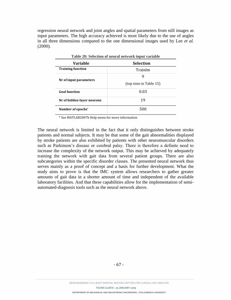
BENCHMARKING FULL-BODY INERTIAL MOTION CAPTURE FOR CLINICAL GAIT ANALYSIS
TEUNIS CLOETE - 29 JANUARY 2009
DEPARTMENT OF MECHANICAL AND MECHATRONIC ENGINEERING - STELLENBOSCH UNIVERSITY
- 67 -
regression neural network and joint angles and spatial parameters from still images as
input parameters. The high accuracy achieved is most likely due to the use of angles
in all three dimensions compared to the one dimensional images used by Lee et al.
(2000).
Table 20: Selection of neural network input variable
Variable Selection Training function Trainlm
Nr of input parameters 9
(top nine in Table 15)
Goal function 0.03
Nr of hidden-layer neurons 19
Number of epochs* 500
* See MATLAB2007b Help menu for more information
The neural network is limited in the fact that it only distinguishes between stroke
patients and normal subjects. It may be that some of the gait abnormalities displayed
by stroke patients are also exhibited by patients with other neuromuscular disorders
such as Parkinson’s disease or cerebral palsy. There is therefore a definite need to
increase the complexity of the network output. This may be achieved by adequately
training the network with gait data from several patient groups. There are also
subcategories within the specific disorder classes. The presented neural network thus
serves mainly as a proof of concept and a basis for further development. What the
study aims to prove is that the IMC system allows researchers to gather greater
amounts of gait data in a shorter amount of time and independent of the available
laboratory facilities. And that these capabilities allow for the implementation of semi-
automated-diagnosis tools such as the neural network above.
BENCHMARKING FULL-BODY INERTIAL MOTION CAPTURE FOR CLINICAL GAIT ANALYSIS
TEUNIS CLOETE - 29 JANUARY 2009
DEPARTMENT OF MECHANICAL AND MECHATRONIC ENGINEERING - STELLENBOSCH UNIVERSITY
- 68 -
6. CONCLUSION
6.1. Using full-body IMC in everyday activities
From Section 2.1.3.2 and Appendix C it is apparent that the IMC system is slightly
sensitive to local magnetic disturbances. Built-in algorithms are only able to
compensate for these disturbances for short periods of time by reducing the work of
the magnetometer readings in the correction filter. It is therefore essential to ask what
effect this limitation has on the use of IMC in clinical gait analysis.
Firstly, the environments in which clinical gait analysis is employed and the
associated equipment were considered. In most cases gait studies are performed
within laboratories, hospitals or clinics. Gait laboratories often contain specially
adapted walkways in which force-plates are housed. These housings may be
constructed using ferrous metal which will lead to EMI. Force plates may also affect
readings. These problems can however be eliminated by employing wooden floor
mountings and special non interfering force-plates. Most hospitals and clinics contain
equipment which may cause EMI. Wires, metal water pipes and steel construction
material inside floors are also cause for concern. In both the validity and repeatability
studies conducted with the IMC system, steps were taken to avoid the presence of
magnetic disturbances. This included removing any metal and electrical objects
within a 3 m radius of the test area. Before testing commenced the area was tested for
EMI using the IMC system which displays a red dot on the screen if there are
significant magnetic disturbances.
The evaluated IMC system also compensates for magnetic interference for periods of
up to 30 seconds. In a normal gait analysis this would be sufficient. It must however
be stated that the calibration procedure should be done in an EMI-free area. Also
between trials, uncompensated orientation drift may diminish the accuracy of the
system calibration which would lead to reduced between-trial repeatability. These
errors were avoided by frequent recalibration of the IMC system.
Another consideration is that of the gait analysis itself. Clinicians often require the
use of stairs, chairs and treadmills to assess the gait of a patient. The latter is of most
concern as they make use of electric motors to drive the belt. These motors use
electromagnetic fields to drive the motors which lead to definite disturbances in local
magnetic fields. Mills et al. (2007) conducted gait analysis on ten subjects using a
treadmill and EMC which is more sensitive to magnetic disturbances than IMC. They
used a specially designed treadmill with non-metallic rollers and with the motor
located away from the walking surface.
In all the above-mentioned scenarios, careful planning of the measuring environment
and appropriate selection of apparatus could eliminate the limitations associated with
BENCHMARKING FULL-BODY INERTIAL MOTION CAPTURE FOR CLINICAL GAIT ANALYSIS
TEUNIS CLOETE - 29 JANUARY 2009
DEPARTMENT OF MECHANICAL AND MECHATRONIC ENGINEERING - STELLENBOSCH UNIVERSITY
- 69 -
IMC. Force-plates and EMG equipment exist, which could easily be combined with
the IMC system.
What sets IMC apart from other technologies however, is its ability to measure
patients in any environment, inside and outside. This opens the door for its usefulness
in the patient’s everyday living environment as well as in telemedicine applications
which are discussed in the next section.
6.2. Telemedicine
Telemedicine is a term which describes the idea of taking medical services to areas
and communities who are unable to travel to urban areas. This concept is of special
importance to a country such as South Africa in which this study was conducted. The
use of IMC in clinical gait analysis would mean that persons who were previously
unable to afford the use of gait laboratories can now be analysed in their local clinic
or even at home. The IMC system used is compact, lightweight and relatively
affordable. A physician is therefore able to go to a specific area and conduct gait
studies on several patients in a relatively short period of time. Alternatively, rural
clinics may acquire an IMC system with which unskilled clinicians may make gait
recordings and send these via internet streaming or email to a qualified physician.
6.3. Inertial motion capture for clinical gait analysis
To conclude, the objectives of this study were to investigate the validity and
repeatability of IMC in the context of clinical gait analysis. This is motivated by the
fact that this technology is still largely untested and therefore underutilized in clinical
applications. It was found that currently used kinematic gait measuring systems are
mostly bound to laboratory use and therefore relatively costly and time consuming.
They lack versatility and mobility which is increasingly required from such a system.
In order to gain the trust in IMC from physicians and researchers, research studies
such as this one is required which quantitatively compare IMC to proven and mature
technologies.
To this end, validity and repeatability studies were conducted using a commercially
available full-body IMC system. Validity study results showed good correlation
between kinematic joint angles in the sagittal and frontal planes for the knees and
hips and acceptable comparison in the transverse planes of these joints. The ankle
joint angles proved less comparable with average validly results. Discrepancies were
accounted to a combination of factors including a misalignment of rotation axes and
non-ideal design of the IMC system foot sensor.
Repeatability study results on the other hand were excellent when compared to
similar studies using OMC and EMC. Within-day repeatability of IMC measured
BENCHMARKING FULL-BODY INERTIAL MOTION CAPTURE FOR CLINICAL GAIT ANALYSIS
TEUNIS CLOETE - 29 JANUARY 2009
DEPARTMENT OF MECHANICAL AND MECHATRONIC ENGINEERING - STELLENBOSCH UNIVERSITY
- 70 -
results was higher than that recorded using OMC for both frontal and transverse plane
angles of all three joint pairs. The sagital plane repeatability performed slightly better
in OMC tests. Within-day values recorded using EMC were in most cases slightly
higher than those recoded for the IMC system, however the within-day repeatability
using IMC was high across the board. Between-day repeatability seems to be where
the strength of the IMC system lies. Results show that the IMC system has, for most
of the analysed joint angles, superior between-day repeatability when compared to
both the OMC and EMC systems. It may therefore be concluded that the IMC system
produces repeatable kinematic joint angles patterns from one test day to the next. This
is of greater use in rehabilitation studies where changes in gait patterns due to
improvements in locomotion are generally small.
Temporal-spatial repeatability was not as good as that of the joint kinematics because
of limitations in gait phase identification algorithms, however repeatability values
were acceptable for use in clinical gait analysis. Again, a greater degree of
repeatability was found in between-day tests than in within-day tests.
Finally an ealuation was made in Section 5 of the diagnostic potential of IMC in a
clinical application. Here a neural network was trained and tested using gait
parameters from stroke patients and able-bodied subjects in an attempt to
automatically distinguish between these two groups. The selected network was tested
for repeatability and based on this the network input variables were selected. The
result section was a neural network that was 99.4% accurate in determining whether a
measured stride came from an able-bodied subject or a stroke patient.
It is therefore concluded that the commercially available, full-body IMC system is
suited for use in clinical gait assessments, not only in conventional laboratory tests
but also in adverse and rural environments. The tested system is user-friendly,
requires little time for calibration and testing, is relatively inexpensive and can easily
be combined with semi-automatic diagnosis methods. These aspects address
limitations stated by Simon (2004) which have lead to the under-utilization of gait
analysis in general patient care.
6.4. Recommendations
Further analysis into the definition of the ankle joint axis is required for both the
OMC and IMC systems to determine the root of this difference. In the same context,
refinement of the spatial gait phase identification algorithm should be done to better
match the heel-strike and toe-off instances found with real values. This may also lead
to improved step length calculation.
BENCHMARKING FULL-BODY INERTIAL MOTION CAPTURE FOR CLINICAL GAIT ANALYSIS
TEUNIS CLOETE - 29 JANUARY 2009
DEPARTMENT OF MECHANICAL AND MECHATRONIC ENGINEERING - STELLENBOSCH UNIVERSITY
- 71 -
Improvements of the IMC system foot sensor may include: reducing the sensor size,
creating a rounded sensor base adapted to the shape of the foot, or placing the sensor
cable attachment on another side of the sensor.
6.5. Future work
The IMC system allows for relatively quick and simple collection of vast amounts of
gait data. This includes data from patients and controls. With this in mind a study
may be conducted in which a neural network may be trained and tested for a wider
variety of gait pathologies. The network could for example distinguish between
patients with CP, PD or stroke. A network such as that would be of great use in
telemedicine to determine the treatment required for patients without them having to
incur the costs involved in travelling to urban areas and seeing a specialist face-to-
face.
Another study may combine motion capture with the measure of other physiological
parameters in a self-contained bio-measurement suit. The applications of such a suit
are endless, especially in sports, medicine and ergonomic studies.

BENCHMARKING FULL-BODY INERTIAL MOTION CAPTURE FOR CLINICAL GAIT ANALYSIS
TEUNIS CLOETE - 29 JANUARY 2009
DEPARTMENT OF MECHANICAL AND MECHATRONIC ENGINEERING - STELLENBOSCH UNIVERSITY
- 72 -
References
BENCHMARKING FULL-BODY INERTIAL MOTION CAPTURE FOR CLINICAL GAIT ANALYSIS
TEUNIS CLOETE - 29 JANUARY 2009
DEPARTMENT OF MECHANICAL AND MECHATRONIC ENGINEERING - STELLENBOSCH UNIVERSITY
- R1 -
7. REFERENCES
Aminian, K., Najafi, B., Büla, C., Leyvraz, P., and Robert, P. (2001). Ambulatory gait
analysis using gyroscopes. In: American Society of Biomechanics Annual Meeting, 2001.
San Diego.
Ascension Technology Corporation. (2007). MotionStar Wireless® 2. [online]. [Accessed 17
September 2008]. Available form World Wide Web: http://www.ascension-
tech.com/products/motionstarwireless.php
Bachmann, E. R. (2000). Inertial and Magnetic Tracking of Limb Segment Orientation for
Inserting Humans Into Synthetic Environments.,. Monterey, California.
Baker, R. (2007). The history of gait analysis before the advent of modern computers. Gait
and Posture,Vol. 26(3), pp.331-342.
Besier, T. F., Sturnieks, D. L., Alderson, J. A., and Lloyd, D. G. (2003). Repeatability of gait
data using a functional hip joint centre and a mean helical knee axis. Journal of
Biomechanics,Vol. 36, pp.1159-1168.
Boulgouris, N. V., Hatzinakos, D., and Plataniotis, K. N. (2005). Gait Recognition: A
challenging signal processing technology for biometric identification. IEEE Signal
Processing Magazine, November, pp.78-90.
Bronner, S. (undated). Instrumented Analysis of Human Motion. [online]. [Accessed 2
November 2007].
Chen, G., Patten, C., Kothari, D. H., and Zajac, F. E. (2005). Gait differences between
individuals with post-stroke hemiparesis and non-disabled controls at matched speeds. Gait
& Posture,Vol. (22), pp.51-56.
Corazza, S., Mündermann, L., and Andriacchi, T. (2006). Markerless Motion Capture
Methods for Estimation of Human Body Kinematics. In: International symposium on the
3D analysis of human motion, 2006. Valenciennes, France.
Dejnabadi, H., Jolles, B. M., and Aminian, K. (2005). A New Approach to Accurate
Measurement of Uniaxial Joint Angles Based on a Combination of Accelerometers and
Gyroscopes. In: IEEE, (ed). IEEE Transactions on Biomechanical Engineering, 2005.,
pp.1478-1484.
Dejnabadi, H., Jolles, B. M., Casanova, E., Fua, P., and Aminian, K. (2006). Estimation and
Visualization of Sagittal Kinematics of Lower Limb Orientation Using Body-Fixed
Sensors. In: IEEE, (ed). IEEE Transactions on Biomechanical Engineering, 2006., pp.1385-
1393.
BENCHMARKING FULL-BODY INERTIAL MOTION CAPTURE FOR CLINICAL GAIT ANALYSIS
TEUNIS CLOETE - 29 JANUARY 2009
DEPARTMENT OF MECHANICAL AND MECHATRONIC ENGINEERING - STELLENBOSCH UNIVERSITY
- R2 -
Den Otter, A. R., Geurts, A. C. H., Mulder, T., and Duysens, J. (2007). Abnormalities in the
temporal patterning of lower extremity muscle activity in hemiparetic gait. Gait &
Posture,Vol. (25), pp.342-352.
Diebel, J. (2006). Representing Attitude: Euler Angles, Unit Quaternions, and Rotation
Vectors. Stanford: Stanford University.
Ebersbach, G., Sojer, M., Valleoriola, F., Wissel, J., Müller, J., Tolosa, E., and Poewe, W.
(1999). Comparitive analysis of gait in Parkinson's disease, cerebellar ataxia and subcortical
arterioscerotic encephalopathy. Brain,Vol. 122, pp.1349-1355.
Ephanov, A. and Hurmuzlu, Y. (2001). Generating Pathological Gait Patterns via the Use of
Robotic Locomotion Models. [online]. [Accessed 19 January 2007]. Available form World
Wide Web: http://engr.smu.edu/me/syslab/papers/Simul_Pathology.pdf
Favre, J., Aissaoui, R., Jolles, B. M., Siegrist, O., de Gruise, J. A., and Aminian, K. (2006).
3D joint rotation measurement using MEMs inertial sensors: Application to the knee joint.
In: International symposium on the 3D analysis of human motion , 2006. Valenciennes,
France.
Flavin, P. (1999). Bipedal Human Gait: A 3d Interactive Model with Animation. [online].
[Accessed 2 January 2007].
Frey, W., Zyda, M., Mcghee, R., and Cockayne, B. (1996). Off-the-shelf, real-time, human
body motion capture for synthetic environments. California.
Garg, V. (undated). Gait disturbances. [online]. [Accessed 31 May 2007]. Available form
World Wide Web: http://pain.health.ivillage.com/armlegpain/gaitdisturbances3.cfm
Gök, H., Ergin, S., and Yavuzer, G. (2002). Kinetic and kinematic characteristics of gait in
patients with medial knee arthrosis. Acta Orthop Scand,Vol. 73(6), pp.647-652.
Han, J., Jeon, H. S., Jeon, B. S., and Park, K. S. (2006). Gait detection from three dimentional
acceleration signals of ankles for tha patient with Parkinson's disease. In: ITAB, 2006.
Ioannina, Epirus.
Huhn, K. (undated). An overview of instrumentad gait analysis. [online]. [Accessed 20 June
2007]. Available form World Wide Web:
http://www.umdnj.edu/idsweb/tech_reviews/Karen/.
International Society of Biomechanics. (2002). Letter to the editor. Journal of
Biomechanics,Vol. 35, pp.543-548.
Kadaba, M. P., Ramakrishnan, H. K., Wootten, M. E., Gainey, J., Gorton, G., and Cochran,
G. V. B. (1989). Repeatability of Kinematic, Kinetic, and Elevtromyographic Data in
Normal Adult Gait. Journal of Orthopedic Research,Vol. 7, pp.849-860.

BENCHMARKING FULL-BODY INERTIAL MOTION CAPTURE FOR CLINICAL GAIT ANALYSIS
TEUNIS CLOETE - 29 JANUARY 2009
DEPARTMENT OF MECHANICAL AND MECHATRONIC ENGINEERING - STELLENBOSCH UNIVERSITY
- R3 -
Kim, C. M. and Eng, J. J. (2004). Magnitude and pattern of 3D kinematic and kinetic gait
profiles in persons with stroke: relationship to walking speed. Gait and Posture,Vol. (20),
pp.140-146.
Lackovic, I., Bilas, V., Santic, A., and Nikolic, V. (2000). Measuring of gait parameters from
free moving subjects. Measurement,Vol. 27, pp.121-131.
Lee, H., Guan, L., and Burne, J. A. (2000). Human gait and posture analysis for diagnosing
neurological disorders. In: International Conference on Image Processing, 2000., pp.435-
438.
Lucchetti, L., Cappozzo, A., Cappello, A., and Della Croce, U. (1998). Skin movement
artifact assessment and compensation in the estimation of knee-joint kinematics. Journal of
Biomechanics,Vol. 31, pp.977-984.
Luinge, H. J. (2002). Inertial Sensing of Human Movement. Twente: Univercity of Twente.
Luinge, H. J. and Veltink, P. H. (2005). Measuring orientation of human body segmants
using miniature gyroscopes and accelerometers. Medical and Biological Engineering and
Computing,Vol. 43, pp.273-282.
Mackey, A. H., Walt, S. E., Lobb, G. A., and Stott, N. S. (2005). Reliability of upper and
lower limb three-dimentional kinematics in children with hemiplegia. Gait and
Posture,Vol. 22, pp.1-9.
Mdlanzi, L., Marwala, T., Stander, C. J., Scheffer, C., and Heyns, P. S. (2007). Principal
component analysis and automatic relevance determination in damage identification.
[online]. [Accessed 29 September 2008]. Available form World Wide Web:
http://arxiv.org/abs/0705.1672
MIE Medical Research Ltd. (undated). Gait analysis system. [online]. [Accessed 3 April
2007]. Available form World Wide Web: http://www.mie-uk.com/gait/index.htm
Miller, N., Jenkins, O. C., Kallmann, M., and Matarić, M. J. (2004). Motion capture from
inertial sensing for untethered humanoid teleoperation. In: 4th IEEE/RAS International
Conference on Humanoid Robots, 10 Nov 2004. World Scientific Publishing Company,
pp.547-565.
Mills, P. M., Morrison, S., Lloyd, D. G., and Barrett, R. S. (2007). Repeatability of 3D gait
kinematics obtained from an electromagnetid tracking system during treadmill locomotion.
Journal of Biomechanics,Vol. (40), pp.1504-1511.
Molson Medical Informatics. (1999). Normal Gait. [online]. [Accessed 3 April 2007].
Available form World Wide Web: http://sprojects.mmi.mcgill.ca/gait/normal/intro.asp

BENCHMARKING FULL-BODY INERTIAL MOTION CAPTURE FOR CLINICAL GAIT ANALYSIS
TEUNIS CLOETE - 29 JANUARY 2009
DEPARTMENT OF MECHANICAL AND MECHATRONIC ENGINEERING - STELLENBOSCH UNIVERSITY
- R4 -
Mulroy, S., Gronley, J., Weiss, W., Newsam, C., and Perry, J. (2003). Use of cluster analysis
for gait pattern classification of patients in the early and late recovery phases following
stroke. Gait and Posture,Vol. (18), pp.114-125.
Olney, J. and Richards, C. (1996). Hemiparetic gait following stroke. Part I: Characteristics.
Gait & Posture,Vol. (4), pp.136-148.
Richards, J. (2008). Biomechanics in Clinic and Research. Preston: Elsevier.
Roetenberg, D. (2006). Inertial and Magnetic Sensing of Human Motion. Twente.
Roetenberg, D., Baten, C. T. M., and Veltink, P. H. (2007a). Estimating body segment
orientation by applying inertial and magnetic sensing near ferromagnetic materials. IEEE
Trans Neural Syst Rehabil Eng,Vol. 15(3), pp.469-471.
Roetenberg, D., Luinge, H., and Slycke, P. (2007b). Moven: Full 6DOF Human Motion
Tracking Using Miniture Inertial Sensors. Unpublished.
Roetenberg, D., Slycke, P. J., and Veltink, P. H. (2007c). Ambulatory Position and
Orientation Tracking Fusing Magnetic and Inertial Sensing. IEEE Trans of Biomedical
Engineering,Vol. 54(5), pp.883-890.
Salarian, A., Russmann, H., Vingerhoets, F. J., Dehollain, C., Blanc, Y., Burkhard, P. R., and
Aminian, K. (2004). Gait Assessment in Parkinson's Disease: Toward an Ambulatory
System for Long-Term Monitoring. In: IEEE Transactions on Biomechanical Engineering,
2004., pp.1434-1443.
Simon, S. R. (2004). Quantification of human motion: gait analysis-benefits and limitations
to its application to clinical problems. Journal of Biomechanics,Vol. 37, pp.1869-1880.
Steinwender, G., Saraph, V., Scheiber, S., Zwick, E. B., Uitz, C., and Hackl, K. (2000).
Intrasubject repeatability of gait analysis data in normal and spastic children. Clinical
Biomechanics,Vol. 15, pp.134-139.
Stolse, H., Kuhtz-Buschbeck, J. P., Drücke, H., Jöhnk, K., Illert, M., and Deuschl, G. (2001).
Comparitive analysis of the gait disorder of normal pressure hydrocephalus and Parkinson's
disease. Journal for Neurology, Neurosurgery and Psychiatry,Vol. 70, pp.289-297.
Su, F.-C. and Wu, W.-L. (2000). Design and testing of a generic algorithm neural network in
the assessment of gait patterns. Medical Engineering & Physics,Vol. (22), pp.67-74.
Thies, S. B., Tresadern, P., Kenney, L., Howard, D., Goulermas, J. Y., Smith, C., and Rigby,
J. (2007). Comparison of linear accelerations from three measurement systems during 'reach
& grasp'. Medical Engineering and Physics,Vol. 29(9), pp.967-972.

BENCHMARKING FULL-BODY INERTIAL MOTION CAPTURE FOR CLINICAL GAIT ANALYSIS
TEUNIS CLOETE - 29 JANUARY 2009
DEPARTMENT OF MECHANICAL AND MECHATRONIC ENGINEERING - STELLENBOSCH UNIVERSITY
- R5 -
Vardaxis, V. G., Allard, P., Lachance, R., and Duhaime, M. (1998). Classification of able-
bodied gait using 3-D muscle powers. Human Movement Science,Vol. 17, pp.121-136.
Vlasic, D., Adelsberger, R., Vannucci, G., Barnwell, J., Gross, M., Matusik, W., and
Popović, J. (2007). Practical Motion Capture in Everyday Surroundings. In: ACM
Transactions on Graphics, 2007.
von Acht, V., Bongers, E., Lambert, N., and Verberne, R. (2007). Miniature Wireless Inertial
Sensors for Measuring Human Motion. In: 29th Annual International Conference of the
IEEE EMBS, 2007. Lyon:, pp.6278-6281.
Weisstein, E. W. (undated). Correlation Coefficient. [online]. Available form World Wide
Web: http://mathwolrd.wolfram.com/CorrelationCoefficient.html
Welch, G. and Foxlin, E. (2002). Motion Tracking: No Silver Bullet, but a Respectable
Arsenal. IEEE Computer Graphics and Applications,Vol. 22(6), pp.24-38.
White, S. C., Yack, H. J., and Winter, D. (1989). A three-dimensional musculoskeletal model
for gait analysis. Anatomical variability estimates. Journal of Biomechanics,Vol. 22(8-9),
pp.885-893.
Whiting, W. C. and Rugg, S. (2006). Dynatomy: Dynamic Human Anatomy. USA: Human
Kinematics.
Whittle, M. W. (1996). Clinical gait analysis: A review. Human Motion Science,Vol. 15,
pp.369-387.
Xsens Technologies. (2007). Moven - Inertial motion capturing. [online]. [Accessed 16
March 2007]. Available form World Wide Web:
http://www.xsens.com/index.php?mainmenu=products&submenu=human_motion&subsub
menu=Moven
Xsens Technologies. (2008). Moven. Enschede.
Yavuzer, G., Öken, Ö., Elhan, A., and Stam, H. J. (2006). Repeatability of lower limb three-
dimensional kinematics in patients with stroke. Gait & Posture,Vol. 24(2), pp.S188 - S190.
Zhou, H. and Hu, H. (2004). A Survey - Human Tracking and Stroke Rehabilitation. Essex.

BENCHMARKING FULL-BODY INERTIAL MOTION CAPTURE FOR CLINICAL GAIT ANALYSIS
TEUNIS CLOETE - 29 JANUARY 2009
DEPARTMENT OF MECHANICAL AND MECHATRONIC ENGINEERING - STELLENBOSCH UNIVERSITY
- R6 -
Appendices
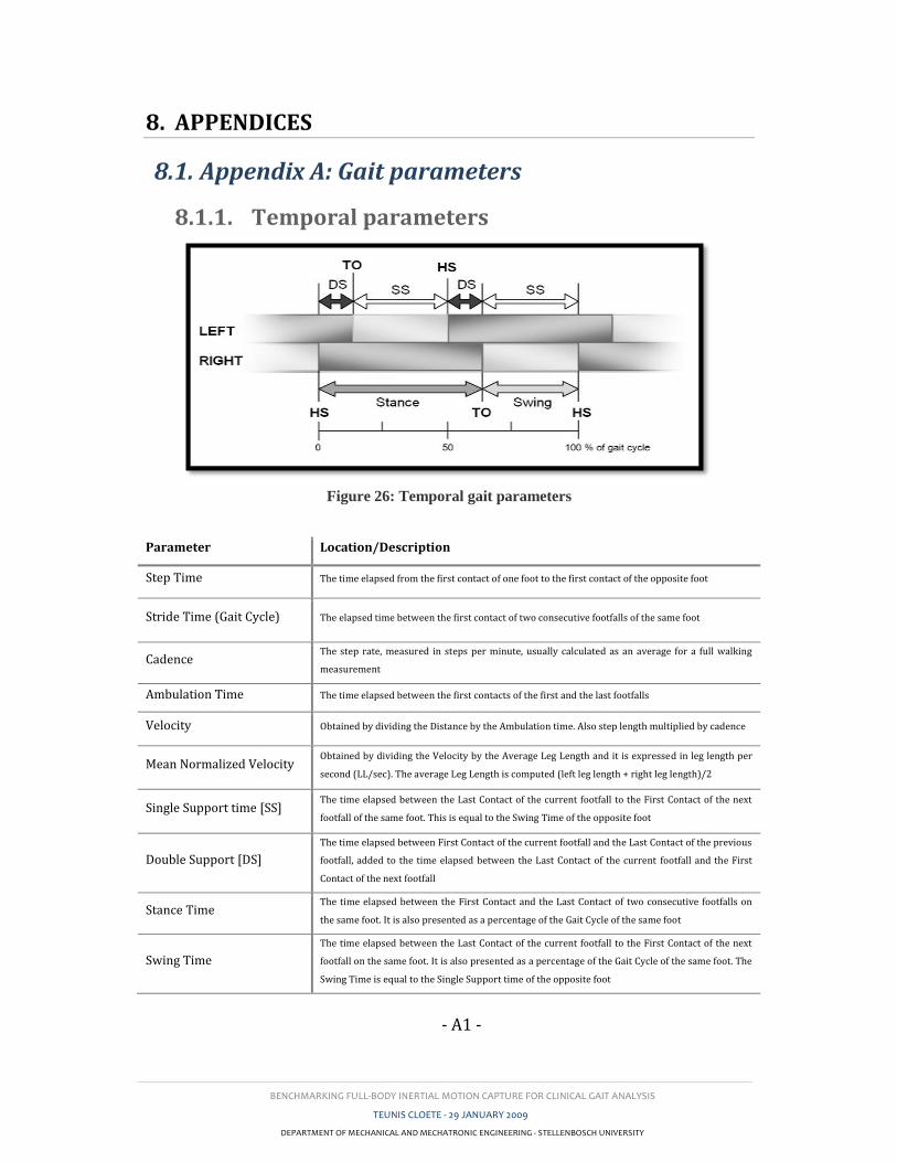
BENCHMARKING FULL-BODY INERTIAL MOTION CAPTURE FOR CLINICAL GAIT ANALYSIS
TEUNIS CLOETE - 29 JANUARY 2009
DEPARTMENT OF MECHANICAL AND MECHATRONIC ENGINEERING - STELLENBOSCH UNIVERSITY
- A1 -
8. APPENDICES
8.1. Appendix A: Gait parameters
8.1.1. Temporal parameters
Figure 26: Temporal gait parameters
Parameter Location/Description
Step Time The time elapsed from the first contact of one foot to the first contact of the opposite foot
Stride Time (Gait Cycle) The elapsed time between the first contact of two consecutive footfalls of the same foot
Cadence The step rate, measured in steps per minute, usually calculated as an average for a full walking
measurement
Ambulation Time The time elapsed between the first contacts of the first and the last footfalls
Velocity Obtained by dividing the Distance by the Ambulation time. Also step length multiplied by cadence
Mean Normalized Velocity Obtained by dividing the Velocity by the Average Leg Length and it is expressed in leg length per
second (LL/sec). The average Leg Length is computed (left leg length + right leg length)/2
Single Support time [SS] The time elapsed between the Last Contact of the current footfall to the First Contact of the next
footfall of the same foot. This is equal to the Swing Time of the opposite foot
Double Support [DS]
The time elapsed between First Contact of the current footfall and the Last Contact of the previous
footfall, added to the time elapsed between the Last Contact of the current footfall and the First
Contact of the next footfall
Stance Time The time elapsed between the First Contact and the Last Contact of two consecutive footfalls on
the same foot. It is also presented as a percentage of the Gait Cycle of the same foot
Swing Time
The time elapsed between the Last Contact of the current footfall to the First Contact of the next
footfall on the same foot. It is also presented as a percentage of the Gait Cycle of the same foot. The
Swing Time is equal to the Single Support time of the opposite foot
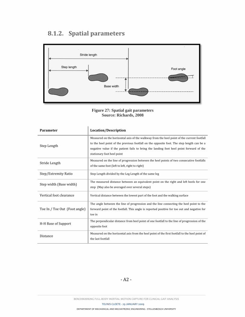
BENCHMARKING FULL-BODY INERTIAL MOTION CAPTURE FOR CLINICAL GAIT ANALYSIS
TEUNIS CLOETE - 29 JANUARY 2009
DEPARTMENT OF MECHANICAL AND MECHATRONIC ENGINEERING - STELLENBOSCH UNIVERSITY
- A2 -
8.1.2. Spatial parameters
Figure 27: Spatial gait parameters
Source: Richards, 2008
Parameter Location/Description
Step Length
Measured on the horizontal axis of the walkway from the heel point of the current footfall
to the heel point of the previous footfall on the opposite foot. The step length can be a
negative value if the patient fails to bring the landing foot heel point forward of the
stationary foot heel point
Stride Length Measured on the line of progression between the heel points of two consecutive footfalls
of the same foot (left to left, right to right)
Step/Extremity Ratio Step Length divided by the Leg Length of the same leg
Step width (Base width) The measured distance between an equivalent point on the right and left heels for one
step (May also be averaged over several steps)
Vertical foot clearance Vertical distance between the lowest part of the foot and the walking surface
Toe In / Toe Out (Foot angle)
The angle between the line of progression and the line connecting the heel point to the
forward point of the footfall. This angle is reported positive for toe out and negative for
toe in
H-H Base of Support The perpendicular distance from heel point of one footfall to the line of progression of the
opposite foot
Distance Measured on the horizontal axis from the heel point of the first footfall to the heel point of
the last footfall
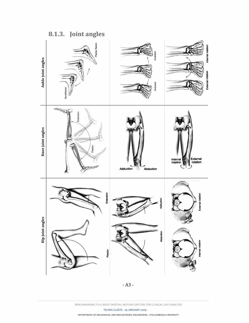
BENCHMARKING FULL-BODY INERTIAL MOTION CAPTURE FOR CLINICAL GAIT ANALYSIS
TEUNIS CLOETE - 29 JANUARY 2009
DEPARTMENT OF MECHANICAL AND MECHATRONIC ENGINEERING - STELLENBOSCH UNIVERSITY
- A3 -
8.1.3. Joint angles A
nk
le j
oin
t a
ng
les
Kn
ee
jo
int
an
gle
s
Hip
jo
int
an
gle
s
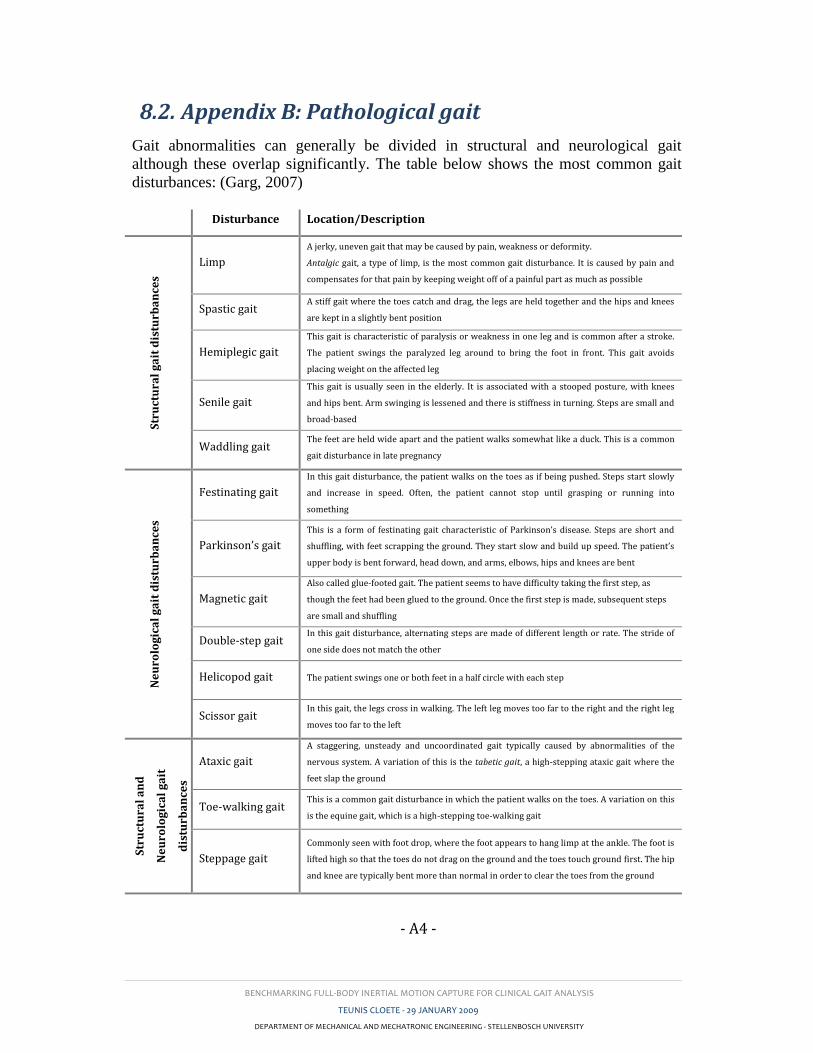
BENCHMARKING FULL-BODY INERTIAL MOTION CAPTURE FOR CLINICAL GAIT ANALYSIS
TEUNIS CLOETE - 29 JANUARY 2009
DEPARTMENT OF MECHANICAL AND MECHATRONIC ENGINEERING - STELLENBOSCH UNIVERSITY
- A4 -
8.2. Appendix B: Pathological gait
Gait abnormalities can generally be divided in structural and neurological gait
although these overlap significantly. The table below shows the most common gait
disturbances: (Garg, 2007)
Disturbance Location/Description
Str
uct
ura
l g
ait
dis
turb
an
ces
Limp
A jerky, uneven gait that may be caused by pain, weakness or deformity.
Antalgic gait, a type of limp, is the most common gait disturbance. It is caused by pain and
compensates for that pain by keeping weight off of a painful part as much as possible
Spastic gait A stiff gait where the toes catch and drag, the legs are held together and the hips and knees
are kept in a slightly bent position
Hemiplegic gait
This gait is characteristic of paralysis or weakness in one leg and is common after a stroke.
The patient swings the paralyzed leg around to bring the foot in front. This gait avoids
placing weight on the affected leg
Senile gait
This gait is usually seen in the elderly. It is associated with a stooped posture, with knees
and hips bent. Arm swinging is lessened and there is stiffness in turning. Steps are small and
broad-based
Waddling gait The feet are held wide apart and the patient walks somewhat like a duck. This is a common
gait disturbance in late pregnancy
Ne
uro
log
ica
l g
ait
dis
turb
an
ces
Festinating gait
In this gait disturbance, the patient walks on the toes as if being pushed. Steps start slowly
and increase in speed. Often, the patient cannot stop until grasping or running into
something
Parkinson’s gait
This is a form of festinating gait characteristic of Parkinson’s disease. Steps are short and
shuffling, with feet scrapping the ground. They start slow and build up speed. The patient’s
upper body is bent forward, head down, and arms, elbows, hips and knees are bent
Magnetic gait
Also called glue-footed gait. The patient seems to have difficulty taking the first step, as
though the feet had been glued to the ground. Once the first step is made, subsequent steps
are small and shuffling
Double-step gait In this gait disturbance, alternating steps are made of different length or rate. The stride of
one side does not match the other
Helicopod gait The patient swings one or both feet in a half circle with each step
Scissor gait In this gait, the legs cross in walking. The left leg moves too far to the right and the right leg
moves too far to the left
Str
uct
ura
l a
nd
Ne
uro
log
ica
l g
ait
dis
turb
an
ces
Ataxic gait
A staggering, unsteady and uncoordinated gait typically caused by abnormalities of the
nervous system. A variation of this is the tabetic gait, a high-stepping ataxic gait where the
feet slap the ground
Toe-walking gait This is a common gait disturbance in which the patient walks on the toes. A variation on this
is the equine gait, which is a high-stepping toe-walking gait
Steppage gait
Commonly seen with foot drop, where the foot appears to hang limp at the ankle. The foot is
lifted high so that the toes do not drag on the ground and the toes touch ground first. The hip
and knee are typically bent more than normal in order to clear the toes from the ground
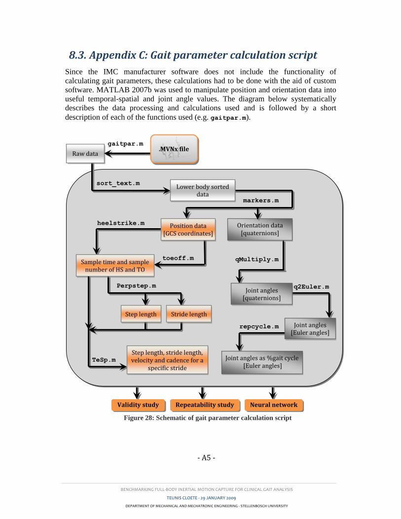
BENCHMARKING FULL-BODY INERTIAL MOTION CAPTURE FOR CLINICAL GAIT ANALYSIS
TEUNIS CLOETE - 29 JANUARY 2009
DEPARTMENT OF MECHANICAL AND MECHATRONIC ENGINEERING - STELLENBOSCH UNIVERSITY
- A5 -
8.3. Appendix C: Gait parameter calculation script
Since the IMC manufacturer software does not include the functionality of
calculating gait parameters, these calculations had to be done with the aid of custom
software. MATLAB 2007b was used to manipulate position and orientation data into
useful temporal-spatial and joint angle values. The diagram below systematically
describes the data processing and calculations used and is followed by a short
description of each of the functions used (e.g. gaitpar.m).
sort_text.m
markers.m
Lower body sorted data
gaitpar.m
heelstrike.m
toeoff.m qMultiply.m
q2Euler.m Joint angles
[quaternions]
Position data [GCS coordinates]
repcycle.m
Perpstep.m
Joint angles as %gait cycle [Euler angles]
Sample time and sample number of HS and TO
Orientation data [quaternions]
Step length Stride length
TeSp.m
Step length, stride length, velocity and cadence for a
specific stride
Validity study Repeatability study Neural network
Raw data .MVNx file
Joint angles [Euler angles]
Figure 28: Schematic of gait parameter calculation script
BENCHMARKING FULL-BODY INERTIAL MOTION CAPTURE FOR CLINICAL GAIT ANALYSIS
TEUNIS CLOETE - 29 JANUARY 2009
DEPARTMENT OF MECHANICAL AND MECHATRONIC ENGINEERING - STELLENBOSCH UNIVERSITY
- A6 -
gaitpar.m
This function was used in each of the three main sections to calculate the required
gait parameters from a specific *.MVNx file. The function controls several sub-
functions as shown in Figure 28. These are described below. Some calculations such
as those for step and stride lengths are completed within this function.
sort_text.m
The Xsens proprietary MVNx file described in Appendix C contains several lines of
initialization parameters as well as miscellaneous data such as the date of recording.
Following these lines of information is a large matrix containing position and
orientation data of each of the 23 body model segments. This function reads this
matrix along with the number of recorded frames and the recording frame-rate.
markers.m
To simplify orientation and position data handling, these values were sorted into
manageable variables named according to the specific segment and a hyphenated p or
q for position and orientation respectively (e.g. the left-foot-segment position and
orientation variables are LF_p and LF_q. Here position variables are three-column
matrices with each row containing the segment position components in the GCS for
each time frame. Orientation variables consist of four-column matrices with each row
consisting of four unit quaternions also in the GCS). As this study focused only on
the lower body gait parameters, only these were sorted for further use.
heelstrike.m
This function uses the position vectors of the feet to calculate the heel-strike
instances. x- and y-plane coordinates are differentiated over time to show when the
respective foot is in motion at a specific time frame. These values of and are
multiplied to produce a plot of velocity vs. time. Values are then forced into binary
form by taking the twelfth power of velocity and then applying a threshold filter. The
exponential multiplication was done to force low values to zero and higher values to
very high values. A threshold was applied with the aid of the peakdet.m built-in
MATLAB function. After this step a running loop was created to find the rising edges
which were taken as the points of heel-strike. This is similar to the approach followed
by Han et al. (2006).
toeoff.m
This function is identical to heelstrike.m except that the falling edges are found and
taken as the points of toe-off.

BENCHMARKING FULL-BODY INERTIAL MOTION CAPTURE FOR CLINICAL GAIT ANALYSIS
TEUNIS CLOETE - 29 JANUARY 2009
DEPARTMENT OF MECHANICAL AND MECHATRONIC ENGINEERING - STELLENBOSCH UNIVERSITY
- A7 -
PerpStep.m
The Vicon OMC calibrates its spatial test volume in such a way that the subject walks
parallel to the y-axis. This simplifies step length calculations as the x-coordinates can
be employed directly. The Moven IMC calibrates to a pose which faces in the
direction of magnetic north. For this reason, a direction vector (simulating the y-axis
of the Vicon) had to be determined. The step and stride lengths were then found by
taking the component of foot displacement parallel to the direction vector.
TeSp.m
As mentioned above, step and stride lengths are calculated within PerpStep.m.
These lengths are calculated for the entire recording. From these values TeSp.m
isolates the step and stride length for a specific studied stride. It also calculates the
velocity and cadence for that specific stride. Velocity is taken as the absolute
displacement of the pelvis from one heel-strike to the next divided by the time
between these consecutive instances. From this cadence is calculated by Cadence =
(Velocity x 60) / Step length.
qMultiply.m
In order to find the segment orientation, the formula, as proposed by Roetenberg,
Luinge and Slycke (2007), was used. In this formula the quaternion multiplication of
the complex conjugate of the proximal segment and the distal segments are calculated
producing the BCS joint angle in quaternion form.
q2Euler.m
Most commercial gait packages represent measured parameters by means of Euler
angles as discussed in Section 3.4.1. This function was therefore employed to convert
joint angles from quaternions to Euler angles using the formula given in Section 3.4.1
by Diebel (2006). The formula was derived for the xyz Cardan sequence also known
as the JCS as proposed by Grood and Suntay (1983).
repcycle.m
Finally a function was required to normalize the joint angles of any given isolated
stride to a percentage of the gait cycle. The function repcycle.m uses the
MATLAB function resample to resample the isolated stride to 100 data point, each
representing 1% of the gait cycle.
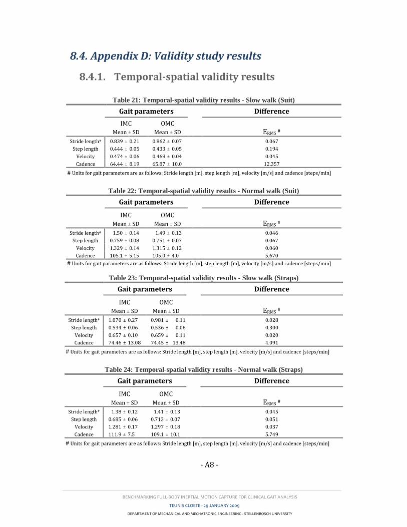
BENCHMARKING FULL-BODY INERTIAL MOTION CAPTURE FOR CLINICAL GAIT ANALYSIS
TEUNIS CLOETE - 29 JANUARY 2009
DEPARTMENT OF MECHANICAL AND MECHATRONIC ENGINEERING - STELLENBOSCH UNIVERSITY
- A8 -
8.4. Appendix D: Validity study results
8.4.1. Temporal-spatial validity results
Table 21: Temporal-spatial validity results - Slow walk (Suit)
Gait parameters
Difference
IMC OMC
Mean ± SD Mean ± SD ERMS #
Stride length# 0.839 ± 0.21 0.862 ± 0.07 0.067
Step length 0.444 ± 0.05 0.433 ± 0.05 0.194
Velocity 0.474 ± 0.06 0.469 ± 0.04 0.045
Cadence 64.44 ± 8.19 65.87 ± 10.0 12.357
# Units for gait parameters are as follows: Stride length [m], step length [m], velocity [m/s] and cadence [steps/min]
Table 22: Temporal-spatial validity results - Normal walk (Suit)
Gait parameters
Difference
IMC OMC
Mean ± SD Mean ± SD ERMS #
Stride length# 1.50 ± 0.14 1.49 ± 0.13 0.046
Step length 0.759 ± 0.08 0.751 ± 0.07 0.067
Velocity 1.329 ± 0.14 1.315 ± 0.12 0.060
Cadence 105.1 ± 5.15 105.0 ± 4.0 5.670
# Units for gait parameters are as follows: Stride length [m], step length [m], velocity [m/s] and cadence [steps/min]
Table 23: Temporal-spatial validity results - Slow walk (Straps)
Gait parameters
Difference
IMC OMC
Mean ± SD Mean ± SD ERMS #
Stride length# 1.070 ± 0.27 0.981 ± 0.11 0.028
Step length 0.534 ± 0.06 0.536 ± 0.06 0.300
Velocity 0.657 ± 0.10 0.659 ± 0.11 0.020
Cadence 74.46 ± 13.08 74.45 ± 13.48 4.091
# Units for gait parameters are as follows: Stride length [m], step length [m], velocity [m/s] and cadence [steps/min]
Table 24: Temporal-spatial validity results - Normal walk (Straps)
Gait parameters
Difference
IMC OMC
Mean ± SD Mean ± SD ERMS #
Stride length# 1.38 ± 0.12 1.41 ± 0.13 0.045
Step length 0.685 ± 0.06 0.713 ± 0.07 0.051
Velocity 1.281 ± 0.17 1.297 ± 0.18 0.037
Cadence 111.9 ± 7.5 109.1 ± 10.1 5.749
# Units for gait parameters are as follows: Stride length [m], step length [m], velocity [m/s] and cadence [steps/min]
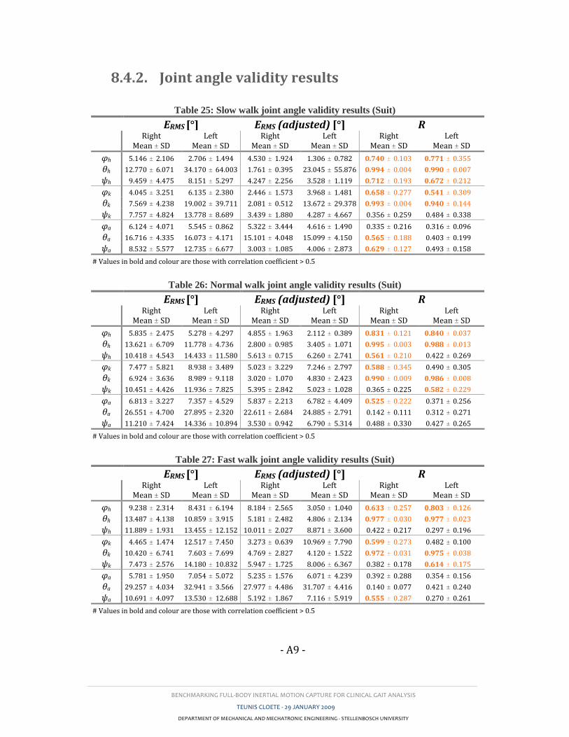
BENCHMARKING FULL-BODY INERTIAL MOTION CAPTURE FOR CLINICAL GAIT ANALYSIS
TEUNIS CLOETE - 29 JANUARY 2009
DEPARTMENT OF MECHANICAL AND MECHATRONIC ENGINEERING - STELLENBOSCH UNIVERSITY
- A9 -
8.4.2. Joint angle validity results
Table 25: Slow walk joint angle validity results (Suit)
ERMS [°] ERMS (adjusted) [°] R
Right Mean ± SD
Left Mean ± SD
Right Mean ± SD
Left Mean ± SD
Right Mean ± SD
Left Mean ± SD
φh 5.146 ± 2.106 2.706 ± 1.494 4.530 ± 1.924 1.306 ± 0.782 0.740 ± 0.103 0.771 ± 0.355
θh 12.770 ± 6.071 34.170 ± 64.003 1.761 ± 0.395 23.045 ± 55.876 0.994 ± 0.004 0.990 ± 0.007
ψh 9.459 ± 4.475 8.151 ± 5.297 4.247 ± 2.256 3.528 ± 1.119 0.712 ± 0.193 0.672 ± 0.212
φk 4.045 ± 3.251 6.135 ± 2.380 2.446 ± 1.573 3.968 ± 1.481 0.658 ± 0.277 0.541 ± 0.309
θk 7.569 ± 4.238 19.002 ± 39.711 2.081 ± 0.512 13.672 ± 29.378 0.993 ± 0.004 0.940 ± 0.144
ψk 7.757 ± 4.824 13.778 ± 8.689 3.439 ± 1.880 4.287 ± 4.667 0.356 ± 0.259 0.484 ± 0.338
φa 6.124 ± 4.071 5.545 ± 0.862 5.322 ± 3.444 4.616 ± 1.490 0.335 ± 0.216 0.316 ± 0.096
θa 16.716 ± 4.335 16.073 ± 4.171 15.101 ± 4.048 15.099 ± 4.150 0.565 ± 0.188 0.403 ± 0.199
ψa 8.532 ± 5.577 12.735 ± 6.677 3.003 ± 1.085 4.006 ± 2.873 0.629 ± 0.127 0.493 ± 0.158
# Values in bold and colour are those with correlation coefficient > 0.5
Table 26: Normal walk joint angle validity results (Suit)
ERMS [°] ERMS (adjusted) [°] R
Right Mean ± SD
Left Mean ± SD
Right Mean ± SD
Left Mean ± SD
Right Mean ± SD
Left Mean ± SD
φh 5.835 ± 2.475 5.278 ± 4.297 4.855 ± 1.963 2.112 ± 0.389 0.831 ± 0.121 0.840 ± 0.037
θh 13.621 ± 6.709 11.778 ± 4.736 2.800 ± 0.985 3.405 ± 1.071 0.995 ± 0.003 0.988 ± 0.013
ψh 10.418 ± 4.543 14.433 ± 11.580 5.613 ± 0.715 6.260 ± 2.741 0.561 ± 0.210 0.422 ± 0.269
φk 7.477 ± 5.821 8.938 ± 3.489 5.023 ± 3.229 7.246 ± 2.797 0.588 ± 0.345 0.490 ± 0.305
θk 6.924 ± 3.636 8.989 ± 9.118 3.020 ± 1.070 4.830 ± 2.423 0.990 ± 0.009 0.986 ± 0.008
ψk 10.451 ± 4.426 11.936 ± 7.825 5.395 ± 2.842 5.023 ± 1.028 0.365 ± 0.225 0.582 ± 0.229
φa 6.813 ± 3.227 7.357 ± 4.529 5.837 ± 2.213 6.782 ± 4.409 0.525 ± 0.222 0.371 ± 0.256
θa 26.551 ± 4.700 27.895 ± 2.320 22.611 ± 2.684 24.885 ± 2.791 0.142 ± 0.111 0.312 ± 0.271
ψa 11.210 ± 7.424 14.336 ± 10.894 3.530 ± 0.942 6.790 ± 5.314 0.488 ± 0.330 0.427 ± 0.265
# Values in bold and colour are those with correlation coefficient > 0.5
Table 27: Fast walk joint angle validity results (Suit)
ERMS [°] ERMS (adjusted) [°] R
Right Mean ± SD
Left Mean ± SD
Right Mean ± SD
Left Mean ± SD
Right Mean ± SD
Left Mean ± SD
φh 9.238 ± 2.314 8.431 ± 6.194 8.184 ± 2.565 3.050 ± 1.040 0.633 ± 0.257 0.803 ± 0.126
θh 13.487 ± 4.138 10.859 ± 3.915 5.181 ± 2.482 4.806 ± 2.134 0.977 ± 0.030 0.977 ± 0.023
ψh 11.889 ± 1.931 13.455 ± 12.152 10.011 ± 2.027 8.871 ± 3.600 0.422 ± 0.217 0.297 ± 0.196
φk 4.465 ± 1.474 12.517 ± 7.450 3.273 ± 0.639 10.969 ± 7.790 0.599 ± 0.273 0.482 ± 0.100
θk 10.420 ± 6.741 7.603 ± 7.699 4.769 ± 2.827 4.120 ± 1.522 0.972 ± 0.031 0.975 ± 0.038
ψk 7.473 ± 2.576 14.180 ± 10.832 5.947 ± 1.725 8.006 ± 6.367 0.382 ± 0.178 0.614 ± 0.175
φa 5.781 ± 1.950 7.054 ± 5.072 5.235 ± 1.576 6.071 ± 4.239 0.392 ± 0.288 0.354 ± 0.156
θa 29.257 ± 4.034 32.941 ± 3.566 27.977 ± 4.486 31.707 ± 4.416 0.140 ± 0.077 0.421 ± 0.240
ψa 10.691 ± 4.097 13.530 ± 12.688 5.192 ± 1.867 7.116 ± 5.919 0.555 ± 0.287 0.270 ± 0.261
# Values in bold and colour are those with correlation coefficient > 0.5
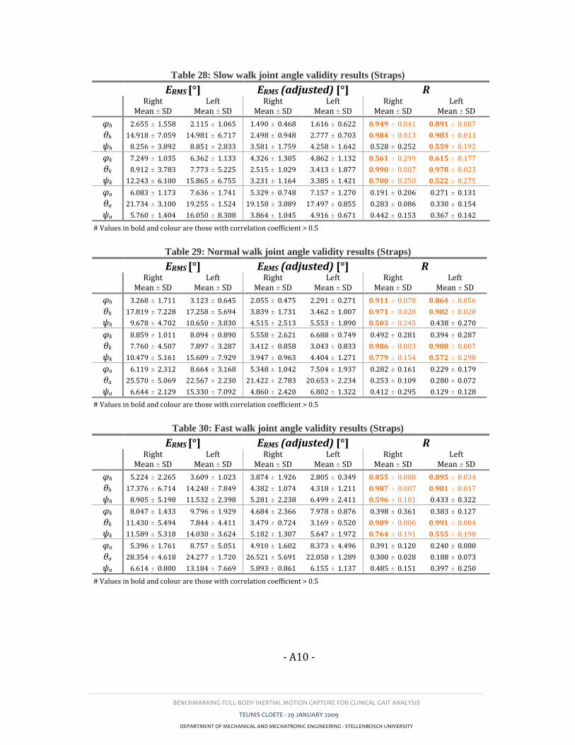
BENCHMARKING FULL-BODY INERTIAL MOTION CAPTURE FOR CLINICAL GAIT ANALYSIS
TEUNIS CLOETE - 29 JANUARY 2009
DEPARTMENT OF MECHANICAL AND MECHATRONIC ENGINEERING - STELLENBOSCH UNIVERSITY
- A10 -
Table 28: Slow walk joint angle validity results (Straps)
ERMS [°] ERMS (adjusted) [°] R
Right Mean ± SD
Left Mean ± SD
Right Mean ± SD
Left Mean ± SD
Right Mean ± SD
Left Mean ± SD
φh 2.655 ± 1.558 2.115 ± 1.065 1.490 ± 0.468 1.616 ± 0.622 0.949 ± 0.041 0.891 ± 0.087
θh 14.918 ± 7.059 14.981 ± 6.717 2.498 ± 0.948 2.777 ± 0.703 0.984 ± 0.013 0.983 ± 0.011
ψh 8.256 ± 3.892 8.851 ± 2.833 3.581 ± 1.759 4.258 ± 1.642 0.528 ± 0.252 0.559 ± 0.192
φk 7.249 ± 1.035 6.362 ± 1.133 4.326 ± 1.305 4.862 ± 1.132 0.561 ± 0.299 0.615 ± 0.177
θk 8.912 ± 3.783 7.773 ± 5.225 2.515 ± 1.029 3.413 ± 1.877 0.990 ± 0.007 0.978 ± 0.023
ψk 12.243 ± 6.100 15.865 ± 6.755 3.231 ± 1.164 3.385 ± 1.421 0.700 ± 0.250 0.522 ± 0.275
φa 6.083 ± 1.173 7.636 ± 1.741 5.329 ± 0.748 7.157 ± 1.270 0.191 ± 0.206 0.271 ± 0.131
θa 21.734 ± 3.100 19.255 ± 1.524 19.158 ± 3.089 17.497 ± 0.855 0.283 ± 0.086 0.330 ± 0.154
ψa 5.760 ± 1.404 16.050 ± 8.308 3.864 ± 1.045 4.916 ± 0.671 0.442 ± 0.153 0.367 ± 0.142
# Values in bold and colour are those with correlation coefficient > 0.5
Table 29: Normal walk joint angle validity results (Straps)
ERMS [°] ERMS (adjusted) [°] R
Right Mean ± SD
Left Mean ± SD
Right Mean ± SD
Left Mean ± SD
Right Mean ± SD
Left Mean ± SD
φh 3.268 ± 1.711 3.123 ± 0.645 2.055 ± 0.475 2.291 ± 0.271 0.911 ± 0.078 0.864 ± 0.056
θh 17.819 ± 7.228 17.258 ± 5.694 3.839 ± 1.731 3.462 ± 1.007 0.971 ± 0.028 0.982 ± 0.020
ψh 9.678 ± 4.702 10.650 ± 3.830 4.515 ± 2.513 5.553 ± 1.890 0.503 ± 0.245 0.438 ± 0.270
φk 8.859 ± 1.011 8.094 ± 0.890 5.558 ± 2.621 6.688 ± 0.749 0.492 ± 0.281 0.394 ± 0.287
θk 7.760 ± 4.507 7.897 ± 3.287 3.412 ± 0.858 3.043 ± 0.833 0.986 ± 0.003 0.988 ± 0.007
ψk 10.479 ± 5.161 15.609 ± 7.929 3.947 ± 0.963 4.404 ± 1.271 0.779 ± 0.154 0.572 ± 0.290
φa 6.119 ± 2.312 8.664 ± 3.168 5.348 ± 1.042 7.504 ± 1.937 0.282 ± 0.161 0.229 ± 0.179
θa 25.570 ± 5.069 22.567 ± 2.230 21.422 ± 2.783 20.653 ± 2.234 0.253 ± 0.109 0.280 ± 0.072
ψa 6.644 ± 2.129 15.330 ± 7.092 4.860 ± 2.420 6.802 ± 1.322 0.412 ± 0.295 0.129 ± 0.128
# Values in bold and colour are those with correlation coefficient > 0.5
Table 30: Fast walk joint angle validity results (Straps)
ERMS [°] ERMS (adjusted) [°] R
Right Mean ± SD
Left Mean ± SD
Right Mean ± SD
Left Mean ± SD
Right Mean ± SD
Left Mean ± SD
φh 5.224 ± 2.265 3.609 ± 1.023 3.874 ± 1.926 2.805 ± 0.349 0.855 ± 0.088 0.895 ± 0.034
θh 17.376 ± 6.714 14.248 ± 7.849 4.382 ± 1.074 4.318 ± 1.211 0.987 ± 0.007 0.981 ± 0.017
ψh 8.905 ± 5.198 11.532 ± 2.398 5.281 ± 2.238 6.499 ± 2.411 0.596 ± 0.181 0.433 ± 0.322
φk 8.047 ± 1.433 9.796 ± 1.929 4.684 ± 2.366 7.978 ± 0.876 0.398 ± 0.361 0.383 ± 0.127
θk 11.430 ± 5.494 7.844 ± 4.411 3.479 ± 0.724 3.169 ± 0.520 0.989 ± 0.006 0.991 ± 0.004
ψk 11.589 ± 5.318 14.030 ± 3.624 5.182 ± 1.307 5.647 ± 1.972 0.764 ± 0.191 0.555 ± 0.198
φa 5.396 ± 1.761 8.757 ± 5.051 4.910 ± 1.602 8.373 ± 4.496 0.391 ± 0.120 0.240 ± 0.080
θa 28.354 ± 4.618 24.277 ± 1.720 26.521 ± 5.691 22.058 ± 1.289 0.300 ± 0.028 0.188 ± 0.073
ψa 6.614 ± 0.800 13.184 ± 7.669 5.893 ± 0.861 6.155 ± 1.137 0.485 ± 0.151 0.397 ± 0.250
# Values in bold and colour are those with correlation coefficient > 0.5
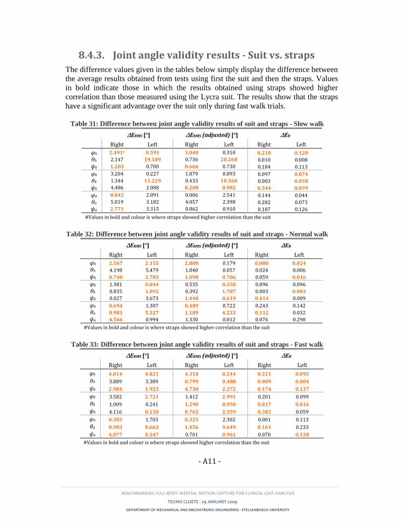
BENCHMARKING FULL-BODY INERTIAL MOTION CAPTURE FOR CLINICAL GAIT ANALYSIS
TEUNIS CLOETE - 29 JANUARY 2009
DEPARTMENT OF MECHANICAL AND MECHATRONIC ENGINEERING - STELLENBOSCH UNIVERSITY
- A11 -
8.4.3. Joint angle validity results - Suit vs. straps
The difference values given in the tables below simply display the difference between
the average results obtained from tests using first the suit and then the straps. Values
in bold indicate those in which the results obtained using straps showed higher
correlation than those measured using the Lycra suit. The results show that the straps
have a significant advantage over the suit only during fast walk trials.
Table 31: Difference between joint angle validity results of suit and straps - Slow walk
∆ERMS [°] ∆ERMS (adjusted) [°] ∆ER
Right Left Right Left Right Left
φh 2.491# 0.591 3.040 0.310 0.210 0.120
θh 2.147 19.189 0.736 20.268 0.010 0.008
ψh 1.203 0.700 0.666 0.730 0.184 0.113
φk 3.204 0.227 1.879 0.893 0.097 0.074
θk 1.344 11.229 0.433 10.260 0.003 0.038
ψk 4.486 2.088 0.208 0.902 0.344 0.039
φa 0.042 2.091 0.006 2.541 0.144 0.044
θa 5.019 3.182 4.057 2.398 0.282 0.073
ψa 2.771 3.315 0.862 0.910 0.187 0.126
#Values in bold and colour is where straps showed higher correlation than the suit
Table 32: Difference between joint angle validity results of suit and straps - Normal walk
∆ERMS [°] ∆ERMS (adjusted) [°] ∆ER
Right Left Right Left Right Left
φh 2.567 2.155 2.800 0.179 0.080 0.024
θh 4.198 5.479 1.040 0.057 0.024 0.006
ψh 0.740 3.783 1.098 0.706 0.059 0.016
φk 1.381 0.844 0.535 0.558 0.096 0.096
θk 0.835 1.092 0.392 1.787 0.003 0.003
ψk 0.027 3.673 1.448 0.619 0.414 0.009
φa 0.694 1.307 0.489 0.722 0.243 0.142
θa 0.981 5.327 1.189 4.233 0.112 0.032
ψa 4.566 0.994 1.330 0.012 0.076 0.298
#Values in bold and colour is where straps showed higher correlation than the suit
Table 33: Difference between joint angle validity results of suit and straps - Fast walk
∆ERMS [°] ∆ERMS (adjusted) [°] ∆ER
Right Left Right Left Right Left
φh 4.014 4.821 4.310 0.244 0.221 0.092
θh 3.889 3.389 0.799 0.488 0.009 0.004
ψh 2.984 1.923 4.730 2.372 0.174 0.137
φk 3.582 2.721 1.412 2.991 0.201 0.099
θk 1.009 0.241 1.290 0.950 0.017 0.016
ψk 4.116 0.150 0.765 2.359 0.382 0.059
φa 0.385 1.703 0.325 2.302 0.001 0.113
θa 0.903 8.663 1.456 9.649 0.161 0.233
ψa 4.077 0.347 0.701 0.961 0.070 0.128
#Values in bold and colour is where straps showed higher correlation than the suit
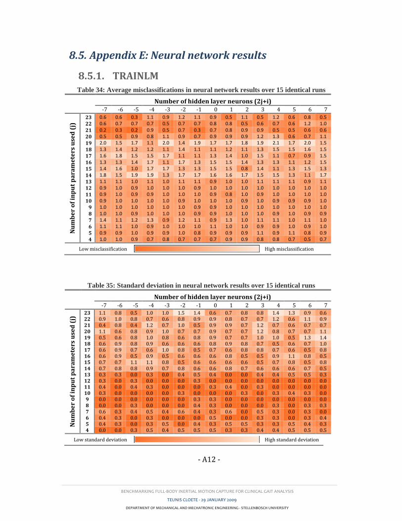
BENCHMARKING FULL-BODY INERTIAL MOTION CAPTURE FOR CLINICAL GAIT ANALYSIS
TEUNIS CLOETE - 29 JANUARY 2009
DEPARTMENT OF MECHANICAL AND MECHATRONIC ENGINEERING - STELLENBOSCH UNIVERSITY
- A12 -
8.5. Appendix E: Neural network results
8.5.1. TRAINLM Table 34: Average misclassifications in neural network results over 15 identical runs
Number of hidden layer neurons (2j+i)
-7 -6 -5 -4 -3 -2 -1 0 1 2 3 4 5 6 7
Nu
mb
er
of
inp
ut
pa
ram
ete
rs u
sed
(j)
23 0.6 0.6 0.3 1.1 0.9 1.2 1.1 0.9 0.5 1.1 0.5 1.2 0.6 0.8 0.5
22 0.6 0.7 0.7 0.7 0.5 0.7 0.7 0.8 0.8 0.5 0.6 0.7 0.6 1.2 1.0
21 0.2 0.3 0.2 0.9 0.5 0.7 0.3 0.7 0.8 0.9 0.9 0.5 0.5 0.6 0.6
20 0.5 0.5 0.9 0.8 1.1 0.9 0.7 0.9 0.9 0.9 1.2 1.3 0.6 0.7 1.1
19 2.0 1.5 1.7 1.1 2.0 1.4 1.9 1.7 1.7 1.8 1.9 2.1 1.7 2.0 1.5
18 1.3 1.4 1.2 1.2 1.1 1.4 1.1 1.1 1.2 1.1 1.3 1.5 1.5 1.6 1.5
17 1.6 1.8 1.5 1.5 1.7 1.1 1.1 1.3 1.4 1.0 1.5 1.1 0.7 0.9 1.5
16 1.3 1.3 1.4 1.7 1.1 1.7 1.3 1.5 1.5 1.4 1.3 1.3 1.1 1.2 1.5
15 1.4 1.6 1.0 1.7 1.7 1.3 1.3 1.5 1.5 0.8 1.4 1.1 1.3 1.5 1.3
14 1.8 1.5 1.9 1.9 1.3 1.7 1.7 1.6 1.6 1.7 1.5 1.5 1.3 1.1 1.7
13 1.1 1.1 1.0 1.1 1.0 1.1 1.1 0.9 1.0 1.0 1.1 1.1 1.1 0.9 1.1
12 0.9 1.0 0.9 1.0 1.0 1.0 0.9 1.0 1.0 1.0 1.0 1.0 1.0 1.0 1.0
11 0.9 1.0 0.9 0.9 1.0 1.0 1.0 0.9 0.8 1.0 0.9 1.0 1.0 1.0 1.0
10 0.9 1.0 1.0 1.0 1.0 0.9 1.0 1.0 1.0 0.9 1.0 0.9 0.9 0.9 1.0
9 1.0 1.0 1.0 1.0 1.0 1.0 0.9 0.9 1.0 1.0 1.0 1.0 1.0 1.0 1.0
8 1.0 1.0 0.9 1.0 1.0 1.0 0.9 0.9 1.0 1.0 1.0 0.9 1.0 0.9 0.9
7 1.4 1.1 1.2 1.3 0.9 1.2 1.1 0.9 1.3 1.0 1.1 1.1 1.0 1.1 1.0
6 1.1 1.1 1.0 0.9 1.0 1.0 1.0 1.1 1.0 1.0 0.9 0.9 1.0 0.9 1.0
5 0.9 0.9 1.0 0.9 0.9 1.0 0.8 0.9 0.9 0.9 1.1 0.9 1.1 0.8 0.9
4 1.0 1.0 0.9 0.7 0.8 0.7 0.7 0.7 0.9 0.9 0.8 0.8 0.7 0.5 0.7
Low misclassification High misclassification
Table 35: Standard deviation in neural network results over 15 identical runs
Number of hidden layer neurons (2j+i)
-7 -6 -5 -4 -3 -2 -1 0 1 2 3 4 5 6 7
Nu
mb
er
of
inp
ut
pa
ram
ete
rs u
sed
(j)
23 1.1 0.8 0.5 1.0 1.0 1.5 1.4 0.6 0.7 0.8 0.8 1.4 1.3 0.9 0.6 22 0.9 1.0 0.8 0.7 0.6 0.8 0.9 0.9 0.8 0.7 0.7 1.2 0.6 1.1 0.9 21 0.4 0.8 0.4 1.2 0.7 1.0 0.5 0.9 0.9 0.7 1.2 0.7 0.6 0.7 0.7 20 1.1 0.6 0.8 0.9 1.0 0.7 0.7 0.9 0.7 0.7 1.2 0.8 0.7 0.7 1.1 19 0.5 0.6 0.8 1.0 0.8 0.6 0.8 0.9 0.7 0.7 1.0 1.0 0.5 1.3 1.4 18 0.6 0.9 0.8 0.9 0.6 0.6 0.6 0.8 0.9 0.8 0.7 0.5 0.6 0.7 1.0 17 0.6 0.9 0.7 0.6 1.0 0.8 0.5 0.7 0.6 0.8 0.8 0.7 0.6 0.5 0.8 16 0.6 0.9 0.5 0.9 0.5 0.6 0.6 0.6 0.8 0.5 0.5 0.9 1.1 0.8 0.5 15 0.7 0.7 1.1 1.1 0.8 0.5 0.6 0.6 0.6 0.6 0.5 0.7 0.8 0.5 0.8 14 0.7 0.8 0.8 0.9 0.7 0.8 0.6 0.6 0.8 0.7 0.6 0.6 0.6 0.7 0.5 13 0.3 0.3 0.0 0.3 0.0 0.4 0.5 0.4 0.0 0.0 0.4 0.4 0.5 0.5 0.3 12 0.3 0.0 0.3 0.0 0.0 0.0 0.3 0.0 0.0 0.0 0.0 0.0 0.0 0.0 0.0 11 0.4 0.0 0.4 0.3 0.0 0.0 0.0 0.3 0.4 0.0 0.3 0.0 0.0 0.0 0.0 10 0.3 0.0 0.0 0.0 0.0 0.3 0.0 0.0 0.0 0.3 0.0 0.3 0.4 0.3 0.0 9 0.0 0.0 0.0 0.0 0.0 0.0 0.3 0.3 0.0 0.0 0.0 0.0 0.0 0.0 0.0 8 0.0 0.0 0.3 0.0 0.0 0.0 0.4 0.3 0.0 0.0 0.0 0.3 0.0 0.3 0.3 7 0.6 0.3 0.4 0.5 0.4 0.6 0.4 0.3 0.6 0.0 0.5 0.3 0.0 0.3 0.0 6 0.4 0.3 0.0 0.3 0.0 0.0 0.0 0.5 0.0 0.0 0.3 0.3 0.0 0.3 0.4 5 0.4 0.3 0.0 0.3 0.5 0.0 0.4 0.3 0.5 0.5 0.3 0.3 0.5 0.4 0.3 4 0.0 0.0 0.3 0.5 0.4 0.5 0.5 0.5 0.3 0.3 0.4 0.4 0.5 0.5 0.5
Low standard deviation High standard deviation
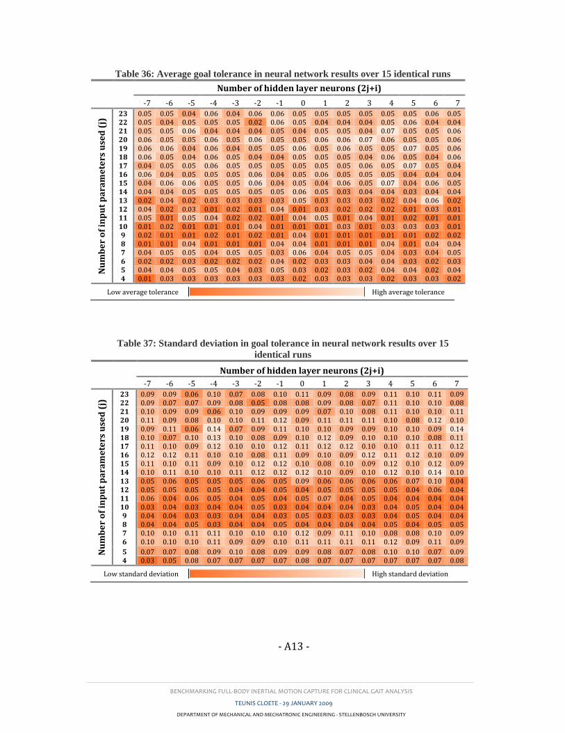
BENCHMARKING FULL-BODY INERTIAL MOTION CAPTURE FOR CLINICAL GAIT ANALYSIS
TEUNIS CLOETE - 29 JANUARY 2009
DEPARTMENT OF MECHANICAL AND MECHATRONIC ENGINEERING - STELLENBOSCH UNIVERSITY
- A13 -
Table 36: Average goal tolerance in neural network results over 15 identical runs
Number of hidden layer neurons (2j+i)
-7 -6 -5 -4 -3 -2 -1 0 1 2 3 4 5 6 7
Nu
mb
er
of
inp
ut
pa
ram
ete
rs u
sed
(j)
23 0.05 0.05 0.04 0.06 0.04 0.06 0.06 0.05 0.05 0.05 0.05 0.05 0.05 0.06 0.05 22 0.05 0.04 0.05 0.05 0.05 0.02 0.06 0.05 0.04 0.04 0.04 0.05 0.06 0.04 0.04 21 0.05 0.05 0.06 0.04 0.04 0.04 0.05 0.04 0.05 0.05 0.04 0.07 0.05 0.05 0.06 20 0.06 0.05 0.05 0.06 0.05 0.06 0.05 0.05 0.06 0.06 0.07 0.06 0.05 0.05 0.06 19 0.06 0.06 0.04 0.06 0.04 0.05 0.05 0.06 0.05 0.06 0.05 0.05 0.07 0.05 0.06 18 0.06 0.05 0.04 0.06 0.05 0.04 0.04 0.05 0.05 0.05 0.04 0.06 0.05 0.04 0.06 17 0.04 0.05 0.05 0.06 0.05 0.05 0.05 0.05 0.05 0.05 0.06 0.05 0.07 0.05 0.04 16 0.06 0.04 0.05 0.05 0.05 0.06 0.04 0.05 0.06 0.05 0.05 0.05 0.04 0.04 0.04 15 0.04 0.06 0.06 0.05 0.05 0.06 0.04 0.05 0.04 0.06 0.05 0.07 0.04 0.06 0.05 14 0.04 0.04 0.05 0.05 0.05 0.05 0.05 0.06 0.05 0.03 0.04 0.04 0.03 0.04 0.04 13 0.02 0.04 0.02 0.03 0.03 0.03 0.03 0.05 0.03 0.03 0.03 0.02 0.04 0.06 0.02 12 0.04 0.02 0.03 0.01 0.02 0.01 0.04 0.01 0.03 0.02 0.02 0.02 0.01 0.03 0.01 11 0.05 0.01 0.05 0.04 0.02 0.02 0.01 0.04 0.05 0.01 0.04 0.01 0.02 0.01 0.01 10 0.01 0.02 0.01 0.01 0.01 0.04 0.01 0.01 0.01 0.03 0.01 0.03 0.03 0.03 0.01 9 0.02 0.01 0.01 0.02 0.01 0.02 0.01 0.04 0.01 0.01 0.01 0.01 0.01 0.02 0.02 8 0.01 0.01 0.04 0.01 0.01 0.01 0.04 0.04 0.01 0.01 0.01 0.04 0.01 0.04 0.04 7 0.04 0.05 0.05 0.04 0.05 0.05 0.03 0.06 0.04 0.05 0.05 0.04 0.03 0.04 0.05 6 0.02 0.02 0.03 0.02 0.02 0.02 0.04 0.02 0.03 0.03 0.04 0.04 0.03 0.02 0.03 5 0.04 0.04 0.05 0.05 0.04 0.03 0.05 0.03 0.02 0.03 0.02 0.04 0.04 0.02 0.04 4 0.01 0.03 0.03 0.03 0.03 0.03 0.03 0.02 0.03 0.03 0.03 0.02 0.03 0.03 0.02
Low average tolerance High average tolerance
Table 37: Standard deviation in goal tolerance in neural network results over 15
identical runs
Number of hidden layer neurons (2j+i)
-7 -6 -5 -4 -3 -2 -1 0 1 2 3 4 5 6 7
Nu
mb
er
of
inp
ut
pa
ram
ete
rs u
sed
(j)
23 0.09 0.09 0.06 0.10 0.07 0.08 0.10 0.11 0.09 0.08 0.09 0.11 0.10 0.11 0.09 22 0.09 0.07 0.07 0.09 0.08 0.05 0.08 0.08 0.09 0.08 0.07 0.11 0.10 0.10 0.08 21 0.10 0.09 0.09 0.06 0.10 0.09 0.09 0.09 0.07 0.10 0.08 0.11 0.10 0.10 0.11 20 0.11 0.09 0.08 0.10 0.10 0.11 0.12 0.09 0.11 0.11 0.11 0.10 0.08 0.12 0.10 19 0.09 0.11 0.06 0.14 0.07 0.09 0.11 0.10 0.10 0.09 0.09 0.10 0.10 0.09 0.14 18 0.10 0.07 0.10 0.13 0.10 0.08 0.09 0.10 0.12 0.09 0.10 0.10 0.10 0.08 0.11 17 0.11 0.10 0.09 0.12 0.10 0.10 0.12 0.11 0.12 0.12 0.10 0.10 0.11 0.11 0.12 16 0.12 0.12 0.11 0.10 0.10 0.08 0.11 0.09 0.10 0.09 0.12 0.11 0.12 0.10 0.09 15 0.11 0.10 0.11 0.09 0.10 0.12 0.12 0.10 0.08 0.10 0.09 0.12 0.10 0.12 0.09 14 0.10 0.11 0.10 0.10 0.11 0.12 0.12 0.12 0.10 0.09 0.10 0.12 0.10 0.14 0.10 13 0.05 0.06 0.05 0.05 0.05 0.06 0.05 0.09 0.06 0.06 0.06 0.06 0.07 0.10 0.04 12 0.05 0.05 0.05 0.05 0.04 0.04 0.05 0.04 0.05 0.05 0.05 0.05 0.04 0.06 0.04 11 0.06 0.04 0.06 0.05 0.04 0.05 0.04 0.05 0.07 0.04 0.05 0.04 0.04 0.04 0.04 10 0.03 0.04 0.03 0.04 0.04 0.05 0.03 0.04 0.04 0.04 0.03 0.04 0.05 0.04 0.04 9 0.04 0.04 0.03 0.03 0.04 0.04 0.03 0.05 0.03 0.03 0.03 0.04 0.05 0.04 0.04 8 0.04 0.04 0.05 0.03 0.04 0.04 0.05 0.04 0.04 0.04 0.04 0.05 0.04 0.05 0.05 7 0.10 0.10 0.11 0.11 0.10 0.10 0.10 0.12 0.09 0.11 0.10 0.08 0.08 0.10 0.09 6 0.10 0.10 0.10 0.11 0.09 0.09 0.10 0.11 0.11 0.11 0.11 0.12 0.09 0.11 0.09
5 0.07 0.07 0.08 0.09 0.10 0.08 0.09 0.09 0.08 0.07 0.08 0.10 0.10 0.07 0.09 4 0.03 0.05 0.08 0.07 0.07 0.07 0.07 0.08 0.07 0.07 0.07 0.07 0.07 0.07 0.08
Low standard deviation High standard deviation
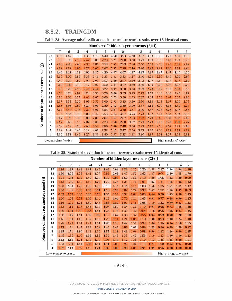
BENCHMARKING FULL-BODY INERTIAL MOTION CAPTURE FOR CLINICAL GAIT ANALYSIS
TEUNIS CLOETE - 29 JANUARY 2009
DEPARTMENT OF MECHANICAL AND MECHATRONIC ENGINEERING - STELLENBOSCH UNIVERSITY
- A14 -
8.5.2. TRAINGDM Table 38: Average misclassifications in neural network results over 15 identical runs
Number of hidden layer neurons (2j+i)
-7 -6 -5 -4 -3 -2 -1 0 1 2 3 4 5 6 7
Nu
mb
er
of
inp
ut
pa
ram
ete
rs u
sed
(j)
23 4.13 4.47 5.33 4.33 4.73 4.40 4.60 3.93 4.20 3.87 4.53 5.00 4.27 3.60 4.13
22 3.33 3.93 2.73 2.47 3.87 2.73 3.27 2.80 3.20 3.73 3.80 3.80 3.13 3.33 3.20
21 2.80 2.80 2.60 2.33 2.80 3.13 2.53 2.93 2.60 2.60 2.60 3.00 2.20 2.07 2.67
20 2.53 2.53 2.07 2.27 2.07 2.67 2.53 2.20 2.40 2.80 2.20 2.67 2.20 2.53 2.60
19 4.40 4.13 4.33 4.00 3.87 4.20 4.07 4.07 4.67 4.67 3.87 4.67 3.47 4.40 4.20
18 3.00 3.00 3.53 3.33 3.40 3.33 3.33 3.33 3.27 3.40 3.20 2.80 3.40 3.00 2.87
17 3.47 3.20 3.07 2.93 2.93 3.67 3.40 2.87 3.20 3.53 3.87 3.67 3.67 2.67 2.87
16 3.00 2.80 3.73 3.47 3.07 3.60 3.47 3.27 3.20 3.60 3.60 3.20 3.07 3.27 3.20
15 2.73 3.20 2.73 2.40 2.40 3.27 3.07 3.00 3.00 3.33 2.73 3.07 3.53 2.53 3.33
14 2.53 3.73 2.87 3.20 3.33 3.20 3.80 3.33 3.13 2.73 3.60 3.33 3.33 3.20 3.07
13 3.00 2.80 3.27 2.40 2.87 3.00 3.73 3.20 2.93 2.87 3.33 2.73 2.47 2.67 2.80
12 3.07 3.33 3.20 2.93 2.53 3.00 2.93 3.13 3.20 2.80 3.20 3.13 2.67 3.00 2.73
11 2.53 2.93 2.60 3.20 3.00 2.80 3.13 3.20 3.00 2.67 3.13 3.00 3.13 2.60 2.27
10 3.07 2.40 2.73 2.20 3.00 3.53 2.87 2.20 2.67 3.00 2.87 3.07 2.73 3.07 2.53
9 3.13 3.53 3.73 3.00 3.27 3.53 3.13 3.07 3.93 2.73 3.07 3.07 2.87 2.93 3.13
8 3.47 2.93 3.33 3.00 2.87 2.87 2.67 2.87 2.53 1.67 2.73 2.40 2.87 2.67 2.80
7 2.67 3.40 3.13 2.87 3.07 2.73 2.60 2.60 3.67 2.73 2.73 3.13 2.73 1.87 2.47
6 3.53 3.13 3.20 2.60 2.53 2.80 2.40 2.40 3.00 2.73 2.47 2.60 2.67 2.73 3.00
5 4.33 4.47 4.47 4.13 4.00 3.33 3.13 3.47 3.00 3.53 3.47 3.00 2.53 2.53 2.33
4 5.00 4.53 3.40 3.27 3.80 3.40 3.07 3.33 3.13 3.60 2.87 2.93 3.27 2.93 2.93
Low misclassification High misclassification
Table 39: Standard deviation in neural network results over 15 identical runs
Number of hidden layer neurons (2j+i)
-7 -6 -5 -4 -3 -2 -1 0 1 2 3 4 5 6 7
Nu
mb
er
of
inp
ut
pa
ram
ete
rs u
sed
(j)
23 1.36 1.88 1.68 1.63 1.62 1.64 2.06 1.39 1.37 2.20 1.88 2.17 2.66 1.64 1.19
22 1.80 2.05 1.28 1.41 1.77 0.88 2.05 1.47 1.52 1.62 1.37 0.94 2.20 1.45 1.70
21 1.21 1.32 1.12 1.45 1.78 1.19 0.83 1.62 1.50 1.18 1.30 1.96 1.42 1.28 0.90
20 1.13 1.36 1.16 1.16 1.22 1.72 1.36 1.26 1.18 1.01 1.82 1.11 1.15 1.06 1.12
19 1.30 2.03 1.23 1.36 1.46 2.40 1.44 1.44 1.11 1.88 1.60 1.35 1.51 1.45 1.47
18 1.00 1.36 0.92 1.05 0.91 1.18 0.90 0.82 1.22 0.99 1.47 1.32 1.50 0.93 0.83
17 0.83 0.68 0.80 0.96 0.70 1.35 0.91 0.99 0.86 0.83 0.64 0.90 1.45 0.98 1.13
16 1.00 1.08 0.59 1.06 1.16 1.18 1.46 0.70 1.21 1.45 0.91 0.77 0.88 0.96 1.15
15 1.16 1.01 1.22 1.30 1.45 0.88 0.80 1.07 0.76 1.68 1.10 1.22 0.99 0.83 1.23
14 1.13 1.10 1.06 1.32 1.72 1.08 1.52 1.35 1.30 1.10 0.91 0.98 0.72 1.26 1.16
13 1.20 0.94 0.88 0.63 1.51 1.25 1.16 1.32 1.22 0.64 1.18 0.96 1.06 0.82 1.15
12 1.58 1.45 1.61 1.39 0.99 1.13 1.62 1.36 1.32 0.56 0.94 0.99 0.90 1.20 1.28
11 1.46 1.33 1.45 1.37 1.36 1.26 0.74 1.21 0.85 1.18 1.30 0.93 1.30 1.24 1.10
10 1.28 0.99 1.44 1.21 1.51 1.96 1.13 1.42 1.50 0.93 1.06 1.16 0.96 1.10 1.55
9 1.13 1.51 1.44 1.56 1.28 1.46 1.41 0.96 2.05 0.96 1.33 0.96 0.99 1.39 0.92
8 1.85 1.71 1.80 1.46 1.30 1.55 1.18 1.41 1.06 0.98 0.96 1.12 1.46 0.90 1.15
7 1.45 1.35 1.19 1.85 1.53 1.39 1.45 1.35 1.63 1.58 1.10 1.13 1.39 1.30 1.13
6 2.13 2.10 1.21 1.35 1.13 0.94 1.18 1.12 1.36 1.10 1.13 1.45 1.35 0.88 1.51
5 1.63 1.30 1.64 0.83 1.41 1.11 0.83 0.92 1.20 1.13 0.74 1.00 0.83 0.92 0.90
4 1.07 2.13 0.99 1.16 1.21 0.83 0.80 0.98 0.83 0.91 0.99 0.96 0.88 0.88 0.80
Low average tolerance High average tolerance
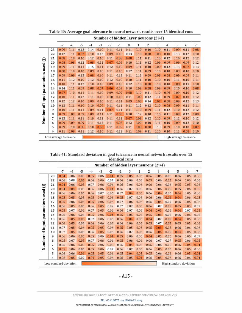
BENCHMARKING FULL-BODY INERTIAL MOTION CAPTURE FOR CLINICAL GAIT ANALYSIS
TEUNIS CLOETE - 29 JANUARY 2009
DEPARTMENT OF MECHANICAL AND MECHATRONIC ENGINEERING - STELLENBOSCH UNIVERSITY
- A15 -
Table 40: Average goal tolerance in neural network results over 15 identical runs
Number of hidden layer neurons (2j+i)
-7 -6 -5 -4 -3 -2 -1 0 1 2 3 4 5 6 7 N
um
be
r o
f in
pu
t p
ara
me
ters
use
d (
j)
23 0.09 0.11 0.13 0.14 0.10 0.11 0.11 0.11 0.10 0.10 0.10 0.11 0.09 0.11 0.08
22 0.12 0.11 0.07 0.10 0.13 0.09 0.10 0.13 0.10 0.08 0.08 0.10 0.13 0.12 0.10
21 0.08 0.10 0.10 0.12 0.10 0.11 0.08 0.08 0.11 0.11 0.10 0.12 0.10 0.12 0.12
20 0.08 0.08 0.12 0.08 0.11 0.07 0.09 0.10 0.11 0.12 0.09 0.09 0.09 0.09 0.12
19 0.09 0.11 0.11 0.15 0.11 0.12 0.10 0.09 0.11 0.10 0.09 0.12 0.13 0.07 0.13
18 0.08 0.10 0.10 0.09 0.10 0.11 0.10 0.12 0.11 0.09 0.10 0.10 0.09 0.10 0.10
17 0.09 0.09 0.12 0.08 0.10 0.11 0.12 0.11 0.12 0.09 0.08 0.08 0.09 0.09 0.11
16 0.11 0.12 0.10 0.12 0.10 0.12 0.10 0.10 0.11 0.10 0.10 0.10 0.11 0.10 0.11
15 0.10 0.11 0.12 0.10 0.10 0.09 0.10 0.12 0.10 0.08 0.10 0.10 0.08 0.11 0.10
14 0.14 0.11 0.09 0.08 0.07 0.06 0.09 0.10 0.09 0.08 0.09 0.09 0.10 0.10 0.08
13 0.07 0.10 0.11 0.11 0.10 0.09 0.09 0.08 0.10 0.11 0.10 0.09 0.09 0.10 0.12
12 0.10 0.11 0.12 0.11 0.10 0.10 0.10 0.11 0.09 0.12 0.11 0.09 0.07 0.10 0.12
11 0.12 0.12 0.10 0.09 0.10 0.11 0.11 0.09 0.08 0.14 0.07 0.08 0.09 0.12 0.13
10 0.12 0.11 0.10 0.10 0.09 0.11 0.11 0.11 0.12 0.12 0.10 0.08 0.09 0.11 0.11
9 0.10 0.11 0.11 0.09 0.11 0.07 0.11 0.11 0.10 0.09 0.11 0.12 0.10 0.12 0.12
8 0.09 0.09 0.09 0.09 0.11 0.11 0.08 0.10 0.12 0.10 0.10 0.11 0.09 0.12 0.09
7 0.13 0.11 0.11 0.10 0.12 0.11 0.11 0.07 0.09 0.12 0.10 0.09 0.12 0.10 0.12
6 0.09 0.09 0.09 0.11 0.12 0.11 0.08 0.12 0.09 0.10 0.11 0.10 0.09 0.12 0.10
5 0.09 0.10 0.08 0.10 0.06 0.11 0.09 0.11 0.08 0.08 0.13 0.09 0.10 0.10 0.07
4 0.11 0.09 0.11 0.12 0.10 0.11 0.12 0.11 0.09 0.11 0.10 0.10 0.11 0.08 0.10
Low average tolerance High average tolerance
Table 41: Standard deviation in goal tolerance in neural network results over 15
identical runs
Number of hidden layer neurons (2j+i)
-7 -6 -5 -4 -3 -2 -1 0 1 2 3 4 5 6 7
Nu
mb
er
of
inp
ut
pa
ram
ete
rs u
sed
(j)
23 0.04 0.06 0.05 0.05 0.06 0.04 0.05 0.05 0.06 0.06 0.05 0.06 0.06 0.06 0.06
22 0.06 0.08 0.05 0.06 0.06 0.07 0.06 0.06 0.06 0.05 0.06 0.05 0.06 0.06 0.06
21 0.04 0.06 0.05 0.07 0.06 0.06 0.06 0.06 0.06 0.06 0.06 0.06 0.05 0.05 0.06
20 0.04 0.04 0.06 0.06 0.06 0.04 0.06 0.07 0.06 0.06 0.06 0.05 0.05 0.06 0.05
19 0.06 0.06 0.06 0.06 0.07 0.06 0.07 0.04 0.05 0.06 0.04 0.06 0.04 0.06 0.06
18 0.05 0.05 0.05 0.05 0.05 0.06 0.05 0.07 0.06 0.06 0.06 0.04 0.04 0.06 0.05
17 0.05 0.06 0.05 0.05 0.06 0.06 0.07 0.06 0.06 0.06 0.05 0.07 0.06 0.06 0.06
16 0.06 0.05 0.06 0.06 0.05 0.07 0.07 0.07 0.06 0.06 0.07 0.05 0.05 0.05 0.07
15 0.05 0.07 0.06 0.07 0.05 0.06 0.06 0.07 0.06 0.04 0.05 0.06 0.04 0.07 0.05
14 0.06 0.06 0.06 0.05 0.06 0.04 0.05 0.05 0.06 0.05 0.05 0.06 0.06 0.06 0.06
13 0.06 0.05 0.05 0.07 0.06 0.06 0.06 0.04 0.06 0.04 0.07 0.05 0.04 0.06 0.06
12 0.06 0.05 0.06 0.06 0.06 0.06 0.06 0.06 0.06 0.05 0.07 0.05 0.05 0.05 0.06
11 0.07 0.05 0.06 0.05 0.05 0.06 0.05 0.05 0.05 0.05 0.03 0.05 0.06 0.06 0.06
10 0.07 0.05 0.06 0.06 0.05 0.06 0.06 0.07 0.06 0.06 0.04 0.05 0.04 0.06 0.06
9 0.06 0.06 0.05 0.05 0.06 0.04 0.05 0.06 0.06 0.04 0.05 0.06 0.06 0.06 0.07
8 0.05 0.07 0.05 0.07 0.06 0.06 0.05 0.06 0.06 0.06 0.07 0.07 0.05 0.06 0.05
7 0.06 0.06 0.05 0.05 0.06 0.06 0.06 0.04 0.06 0.06 0.06 0.06 0.06 0.04 0.04
6 0.05 0.06 0.06 0.05 0.06 0.07 0.06 0.07 0.06 0.06 0.05 0.06 0.06 0.06 0.06
5 0.06 0.06 0.04 0.05 0.05 0.06 0.05 0.04 0.05 0.05 0.06 0.06 0.06 0.05 0.04
4 0.06 0.05 0.07 0.04 0.05 0.06 0.06 0.05 0.04 0.06 0.05 0.06 0.06 0.06 0.04
Low standard deviation High standard deviation
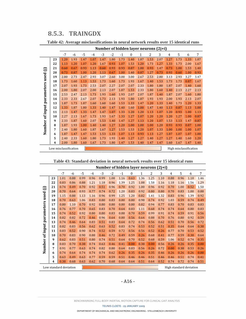
BENCHMARKING FULL-BODY INERTIAL MOTION CAPTURE FOR CLINICAL GAIT ANALYSIS
TEUNIS CLOETE - 29 JANUARY 2009
DEPARTMENT OF MECHANICAL AND MECHATRONIC ENGINEERING - STELLENBOSCH UNIVERSITY
- A16 -
8.5.3. TRAINGDX Table 42: Average misclassifications in neural network results over 15 identical runs
Number of hidden layer neurons (2j+i)
-7 -6 -5 -4 -3 -2 -1 0 1 2 3 4 5 6 7
Nu
mb
er
of
inp
ut
pa
ram
ete
rs u
sed
(j)
23 1.20 1.93 1.47 1.07 1.47 1.80 1.73 1.40 1.87 1.53 2.07 1.27 1.73 1.33 1.87
22 1.13 1.20 1.07 1.20 1.67 0.93 1.07 1.53 1.20 1.73 1.27 1.33 1.73 2.00 1.67
21 0.60 0.67 0.93 1.13 0.60 0.93 0.93 0.87 1.00 0.93 1.47 0.73 1.00 1.53 1.40
20 0.73 0.87 1.00 1.20 1.13 0.67 1.00 1.40 0.87 1.27 0.73 0.93 0.60 1.00 0.93
19 2.80 2.73 2.47 2.93 3.07 2.60 3.00 3.00 2.67 2.53 2.80 3.13 2.93 3.27 3.47
18 1.73 1.60 1.13 1.53 1.73 1.60 1.73 1.93 1.67 1.40 1.53 1.73 1.73 0.87 1.67
17 2.07 1.93 1.73 2.53 2.07 2.27 2.07 2.07 2.33 1.80 1.80 1.87 2.07 1.40 1.60
16 2.00 1.80 2.07 2.00 2.13 2.07 1.87 1.53 2.33 1.80 1.60 1.40 2.13 2.27 2.13
15 2.53 2.47 2.13 1.73 1.93 1.60 1.93 2.07 2.07 1.87 1.40 1.87 2.07 1.60 1.80
14 2.33 2.33 2.67 2.07 1.73 2.13 1.93 1.80 1.87 1.93 1.93 2.00 1.93 2.13 2.07
13 1.87 1.73 1.87 1.60 1.60 1.60 1.53 1.33 1.47 1.20 1.33 1.40 1.73 1.20 1.33
12 1.33 1.87 1.80 1.33 1.40 1.47 1.40 1.60 1.00 1.47 1.40 1.13 0.87 1.13 1.00
11 2.13 1.47 1.33 1.47 1.47 1.07 1.33 1.20 1.20 1.13 1.07 1.20 0.93 1.00 1.13
10 2.27 2.13 1.67 1.73 1.93 1.67 1.33 1.27 1.07 1.20 1.20 1.20 1.27 1.00 0.87
9 2.33 1.87 1.60 2.07 1.53 1.40 1.47 1.27 1.13 1.20 1.07 1.53 1.13 1.47 0.87
8 1.87 1.93 1.00 1.40 1.40 1.27 1.20 1.00 1.00 1.00 1.20 0.93 0.93 0.87 1.00
7 2.40 1.80 1.60 1.87 1.67 1.27 1.53 1.53 1.20 1.07 1.33 1.00 1.00 1.00 1.07
6 1.87 1.47 1.47 1.53 1.53 1.33 1.07 1.13 0.93 1.13 1.27 1.07 1.07 1.07 1.00
5 2.40 2.33 1.60 1.80 1.73 1.93 1.40 1.27 1.27 1.40 1.27 1.27 1.40 1.60 1.20
4 2.00 1.80 1.60 1.67 1.73 1.80 1.47 1.53 1.40 1.47 1.47 1.60 1.67 1.47 1.40
Low misclassification High misclassification
Table 43: Standard deviation in neural network results over 15 identical runs
Number of hidden layer neurons (2j+i)
-7 -6 -5 -4 -3 -2 -1 0 1 2 3 4 5 6 7
Nu
mb
er
of
inp
ut
pa
ram
ete
rs u
sed
(j)
23 1.01 0.88 0.99 0.96 0.99 1.08 1.16 0.63 1.36 1.25 1.10 0.88 0.96 1.18 1.46
22 0.83 0.86 0.88 1.21 1.18 0.96 1.39 1.25 1.08 1.58 1.16 1.18 1.16 1.56 1.29
21 0.74 0.49 0.70 0.92 0.51 0.96 0.70 0.92 1.00 0.96 0.92 0.70 1.00 0.52 1.50
20 0.70 0.64 0.93 0.77 0.74 0.72 1.20 0.83 0.92 0.80 0.80 0.70 0.83 1.00 0.88
19 1.15 0.88 1.13 1.16 0.96 0.99 1.25 1.20 0.82 1.41 1.32 0.83 0.96 1.39 0.92
18 0.70 0.63 1.06 0.83 0.80 0.83 0.80 0.80 0.98 0.74 0.92 1.03 0.59 0.74 0.49
17 0.80 1.10 0.70 0.92 0.80 0.80 0.80 0.80 0.82 0.94 0.77 0.83 0.70 0.83 0.83
16 0.76 0.77 0.70 0.65 0.83 0.70 0.64 0.83 1.11 0.68 0.74 0.74 0.64 0.80 0.83
15 0.74 0.52 0.92 0.80 0.80 0.83 0.88 0.70 0.59 0.99 0.91 0.74 0.59 0.91 0.56
14 0.82 0.82 0.72 0.46 0.96 0.64 0.80 0.56 0.64 0.88 0.70 0.76 0.80 0.92 0.59
13 0.74 0.46 0.64 0.83 0.51 0.83 0.64 0.72 0.74 0.56 0.62 0.51 0.70 0.56 0.72
12 0.82 0.83 0.56 0.62 0.63 0.52 0.83 0.74 0.53 0.52 0.51 0.35 0.64 0.64 0.38
11 0.83 0.52 0.90 0.74 0.52 0.59 0.72 0.56 0.56 0.52 0.26 0.77 0.70 0.53 0.52
10 0.70 0.83 0.90 0.88 0.46 0.72 0.49 0.59 0.26 0.68 0.41 0.77 0.59 0.38 0.64
9 0.62 0.83 0.51 0.80 0.74 0.51 0.64 0.70 0.52 0.68 0.59 1.06 0.52 0.74 0.35
8 0.83 0.70 0.38 0.74 0.63 0.46 0.41 0.00 0.38 0.00 0.56 0.26 0.26 0.35 0.00
7 0.91 0.77 0.63 0.74 0.82 0.80 0.64 0.83 0.56 0.26 0.72 0.00 0.38 0.53 0.26
6 0.74 0.64 0.74 0.74 0.74 0.62 0.26 0.35 0.26 0.35 0.46 0.26 0.26 0.26 0.00
5 0.63 0.49 0.63 0.77 0.59 0.59 0.51 0.46 0.46 0.51 0.46 0.46 0.51 0.74 0.41
4 0.38 0.68 0.63 0.62 0.70 0.68 0.64 0.64 0.51 0.64 0.52 0.74 0.72 0.74 0.51
Low standard deviation High standard deviation
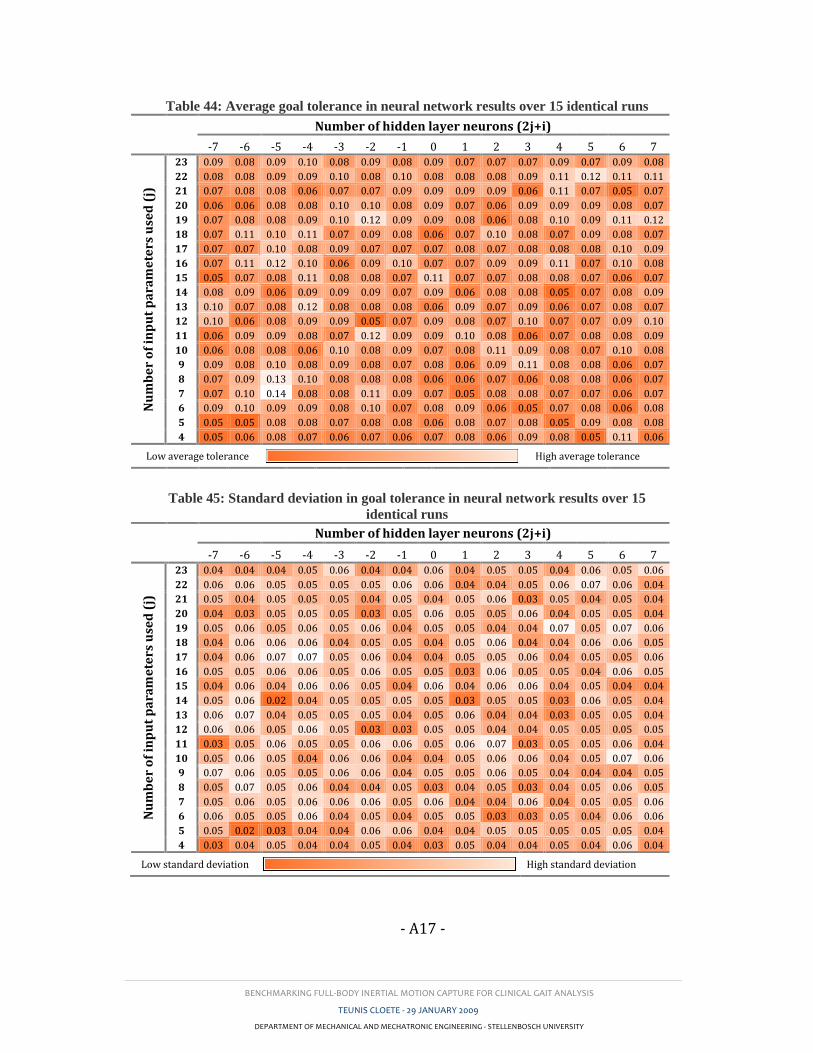
BENCHMARKING FULL-BODY INERTIAL MOTION CAPTURE FOR CLINICAL GAIT ANALYSIS
TEUNIS CLOETE - 29 JANUARY 2009
DEPARTMENT OF MECHANICAL AND MECHATRONIC ENGINEERING - STELLENBOSCH UNIVERSITY
- A17 -
Table 44: Average goal tolerance in neural network results over 15 identical runs
Number of hidden layer neurons (2j+i)
-7 -6 -5 -4 -3 -2 -1 0 1 2 3 4 5 6 7 N
um
be
r o
f in
pu
t p
ara
me
ters
use
d (
j)
23 0.09 0.08 0.09 0.10 0.08 0.09 0.08 0.09 0.07 0.07 0.07 0.09 0.07 0.09 0.08
22 0.08 0.08 0.09 0.09 0.10 0.08 0.10 0.08 0.08 0.08 0.09 0.11 0.12 0.11 0.11
21 0.07 0.08 0.08 0.06 0.07 0.07 0.09 0.09 0.09 0.09 0.06 0.11 0.07 0.05 0.07
20 0.06 0.06 0.08 0.08 0.10 0.10 0.08 0.09 0.07 0.06 0.09 0.09 0.09 0.08 0.07
19 0.07 0.08 0.08 0.09 0.10 0.12 0.09 0.09 0.08 0.06 0.08 0.10 0.09 0.11 0.12
18 0.07 0.11 0.10 0.11 0.07 0.09 0.08 0.06 0.07 0.10 0.08 0.07 0.09 0.08 0.07
17 0.07 0.07 0.10 0.08 0.09 0.07 0.07 0.07 0.08 0.07 0.08 0.08 0.08 0.10 0.09
16 0.07 0.11 0.12 0.10 0.06 0.09 0.10 0.07 0.07 0.09 0.09 0.11 0.07 0.10 0.08
15 0.05 0.07 0.08 0.11 0.08 0.08 0.07 0.11 0.07 0.07 0.08 0.08 0.07 0.06 0.07
14 0.08 0.09 0.06 0.09 0.09 0.09 0.07 0.09 0.06 0.08 0.08 0.05 0.07 0.08 0.09
13 0.10 0.07 0.08 0.12 0.08 0.08 0.08 0.06 0.09 0.07 0.09 0.06 0.07 0.08 0.07
12 0.10 0.06 0.08 0.09 0.09 0.05 0.07 0.09 0.08 0.07 0.10 0.07 0.07 0.09 0.10
11 0.06 0.09 0.09 0.08 0.07 0.12 0.09 0.09 0.10 0.08 0.06 0.07 0.08 0.08 0.09
10 0.06 0.08 0.08 0.06 0.10 0.08 0.09 0.07 0.08 0.11 0.09 0.08 0.07 0.10 0.08
9 0.09 0.08 0.10 0.08 0.09 0.08 0.07 0.08 0.06 0.09 0.11 0.08 0.08 0.06 0.07
8 0.07 0.09 0.13 0.10 0.08 0.08 0.08 0.06 0.06 0.07 0.06 0.08 0.08 0.06 0.07
7 0.07 0.10 0.14 0.08 0.08 0.11 0.09 0.07 0.05 0.08 0.08 0.07 0.07 0.06 0.07
6 0.09 0.10 0.09 0.09 0.08 0.10 0.07 0.08 0.09 0.06 0.05 0.07 0.08 0.06 0.08
5 0.05 0.05 0.08 0.08 0.07 0.08 0.08 0.06 0.08 0.07 0.08 0.05 0.09 0.08 0.08
4 0.05 0.06 0.08 0.07 0.06 0.07 0.06 0.07 0.08 0.06 0.09 0.08 0.05 0.11 0.06
Low average tolerance High average tolerance
Table 45: Standard deviation in goal tolerance in neural network results over 15
identical runs
Number of hidden layer neurons (2j+i)
-7 -6 -5 -4 -3 -2 -1 0 1 2 3 4 5 6 7
Nu
mb
er
of
inp
ut
pa
ram
ete
rs u
sed
(j)
23 0.04 0.04 0.04 0.05 0.06 0.04 0.04 0.06 0.04 0.05 0.05 0.04 0.06 0.05 0.06
22 0.06 0.06 0.05 0.05 0.05 0.05 0.06 0.06 0.04 0.04 0.05 0.06 0.07 0.06 0.04
21 0.05 0.04 0.05 0.05 0.05 0.04 0.05 0.04 0.05 0.06 0.03 0.05 0.04 0.05 0.04
20 0.04 0.03 0.05 0.05 0.05 0.03 0.05 0.06 0.05 0.05 0.06 0.04 0.05 0.05 0.04
19 0.05 0.06 0.05 0.06 0.05 0.06 0.04 0.05 0.05 0.04 0.04 0.07 0.05 0.07 0.06
18 0.04 0.06 0.06 0.06 0.04 0.05 0.05 0.04 0.05 0.06 0.04 0.04 0.06 0.06 0.05
17 0.04 0.06 0.07 0.07 0.05 0.06 0.04 0.04 0.05 0.05 0.06 0.04 0.05 0.05 0.06
16 0.05 0.05 0.06 0.06 0.05 0.06 0.05 0.05 0.03 0.06 0.05 0.05 0.04 0.06 0.05
15 0.04 0.06 0.04 0.06 0.06 0.05 0.04 0.06 0.04 0.06 0.06 0.04 0.05 0.04 0.04
14 0.05 0.06 0.02 0.04 0.05 0.05 0.05 0.05 0.03 0.05 0.05 0.03 0.06 0.05 0.04
13 0.06 0.07 0.04 0.05 0.05 0.05 0.04 0.05 0.06 0.04 0.04 0.03 0.05 0.05 0.04
12 0.06 0.06 0.05 0.06 0.05 0.03 0.03 0.05 0.05 0.04 0.04 0.05 0.05 0.05 0.05
11 0.03 0.05 0.06 0.05 0.05 0.06 0.06 0.05 0.06 0.07 0.03 0.05 0.05 0.06 0.04
10 0.05 0.06 0.05 0.04 0.06 0.06 0.04 0.04 0.05 0.06 0.06 0.04 0.05 0.07 0.06
9 0.07 0.06 0.05 0.05 0.06 0.06 0.04 0.05 0.05 0.06 0.05 0.04 0.04 0.04 0.05
8 0.05 0.07 0.05 0.06 0.04 0.04 0.05 0.03 0.04 0.05 0.03 0.04 0.05 0.06 0.05
7 0.05 0.06 0.05 0.06 0.06 0.06 0.05 0.06 0.04 0.04 0.06 0.04 0.05 0.05 0.06
6 0.06 0.05 0.05 0.06 0.04 0.05 0.04 0.05 0.05 0.03 0.03 0.05 0.04 0.06 0.06
5 0.05 0.02 0.03 0.04 0.04 0.06 0.06 0.04 0.04 0.05 0.05 0.05 0.05 0.05 0.04
4 0.03 0.04 0.05 0.04 0.04 0.05 0.04 0.03 0.05 0.04 0.04 0.05 0.04 0.06 0.04
Low standard deviation High standard deviation

BENCHMARKING FULL-BODY INERTIAL MOTION CAPTURE FOR CLINICAL GAIT ANALYSIS
TEUNIS CLOETE - 29 JANUARY 2009
DEPARTMENT OF MECHANICAL AND MECHATRONIC ENGINEERING - STELLENBOSCH UNIVERSITY
- A18 -


![Inertial Navigation Systems - Indico [Home]indico.ictp.it/event/a12180/session/23/contribution/14/material/0/... · Inertial Navigation Systems. Inertial Navigation Systems ... •](https://img.pdfslide.us/doc/110x75/5a94bdc87f8b9a451b8c1652/inertial-navigation-systems-indico-home-navigation-systems-inertial-navigation.jpg)