Ben M. Chen Associate Professor Office: E4-6-7 Phone: 874 ...uav.ece.nus.edu.sg/~bmchen/courses/ee2462-ppt.pdf · ... solution of Bessel′s equation in terms of Gamma ... wave equation;

1

EE2462 Engineering Math III (Part 1)

Ben M. ChenAssociate Professor

Office: E4-6-7Phone: 874-2289

Email: [email protected]://vlab.ee.nus.edu.sg/~bmchen

2

Course Outline

Series and Power Series: Sequences and series; convergence and

divergence; a test for divergence; comparison tests for positive series; the

ratio test for positive series; absolute convergence; power series.

Special Functions: Bessel′s equation and Bessel functions; the Gamma

function; solution of Bessel′s equation in terms of Gamma function;

Modified Bessel′s equations; Applications of Bessel′s functions;

Legendr′s equation; Legendre polynomials and their properties.

Partial Differential Equations: Boundary value problem in partial

differential equations; wave equation; heat equation; Laplace equation;

Poisson′s equation; Dirichlet and Nuemann Problems. Solutions to wave

and heat equations using method of separation of variables.

Prepared by Ben M. Chen

3

Lectures

Lectures will follow closely (but not 100%) the materials in the lecture

notes (available at http://vlab.ee.nus.edu.sg/~bmchen).

However, certain parts of the lecture notes will not be covered and

examined and this will be made known during the classes.

Attendance is essential.

ASK any question at any time during the lecture.


4

Tutorials

The tutorials will start on Week 4 of the semester (again, tutorial sets can

be downloaded from http://vlab.ee.nus.edu.sg/~bmchen).

Solutions to Tutorial Sets 1, 3 and 4 will be available from my web site

one week after they are conducted. Tutorial Set 2 is an interactive one.

Although you should make an effort to attempt each question before the

tutorial, it is not necessary to finish all the questions.

Some of the questions are straightforward, but quite a few are difficult

and meant to serve as a platform for the introduction of new concepts.

ASK your tutor any question related to the tutorials and the course.


5

Reference Textbooks

• P. V. O′Neil, Advanced Engineering Mathematics, Any Ed., PWS.

• E. Kreyszig, Advanced Engineering Mathematics, Any Ed., Wiley.


6

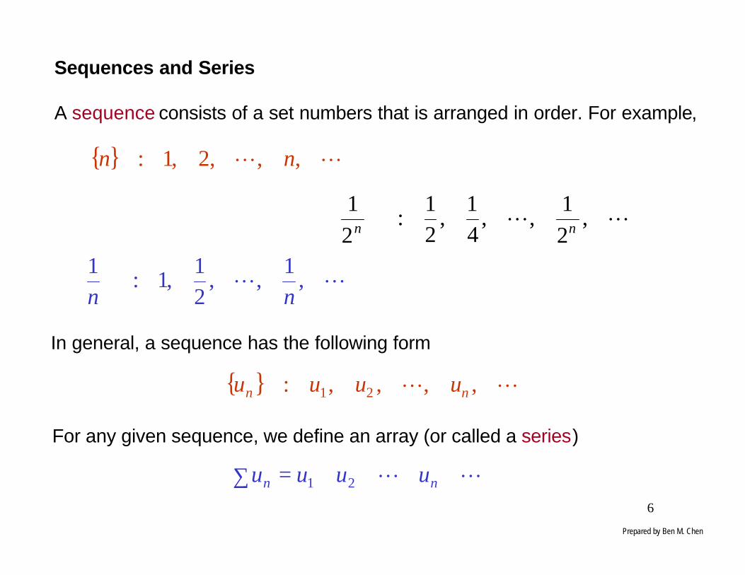
Sequences and Series

A sequence consists of a set numbers that is arranged in order. For example,

{ } LL ,,,2,1: nn

LL ,2

1,,

41

,21

:2

1nn

LL ,1

,,21

,1:1

nn

{ } LL ,,,,: 21 nn uuuu

In general, a sequence has the following form

∑ ++++= LL nn uuuu 21

For any given sequence, we define an array (or called a series)


7

Let us define

This partial sum forms a new sequence { sn }. If, as n increases and tends to

infinity the sequence of numbers sn approaches a finite limit L, we say that

the series

converges. And we write

We say that the infinite series converges to L and that L is the value of the

series. If the sequence does not approach a limit, the series is divergent

and we do not assign any value to it.

n

n

iin uuuus +++== ∑

=L21

1

LL ++++=∑ ni uuuu 21

.lim1

Lusi

inn

== ∑∞

=∞→


8

A Divergence Test

Consider a series

If it converges, then we have

and hence

Thus, if un does not tend to zero as n becomes infinite, the series

is divergent.


.limandlim 1 LsLs nn

nn

== −∞→∞→

0limlim)(limlim 11 =−=−=−= −∞→∞→−∞→∞→LLssssu n

nn

nnn

nn

n


nnnn

n

iin usuuuuus +=++++== −−

=∑ 1121

1

L


9

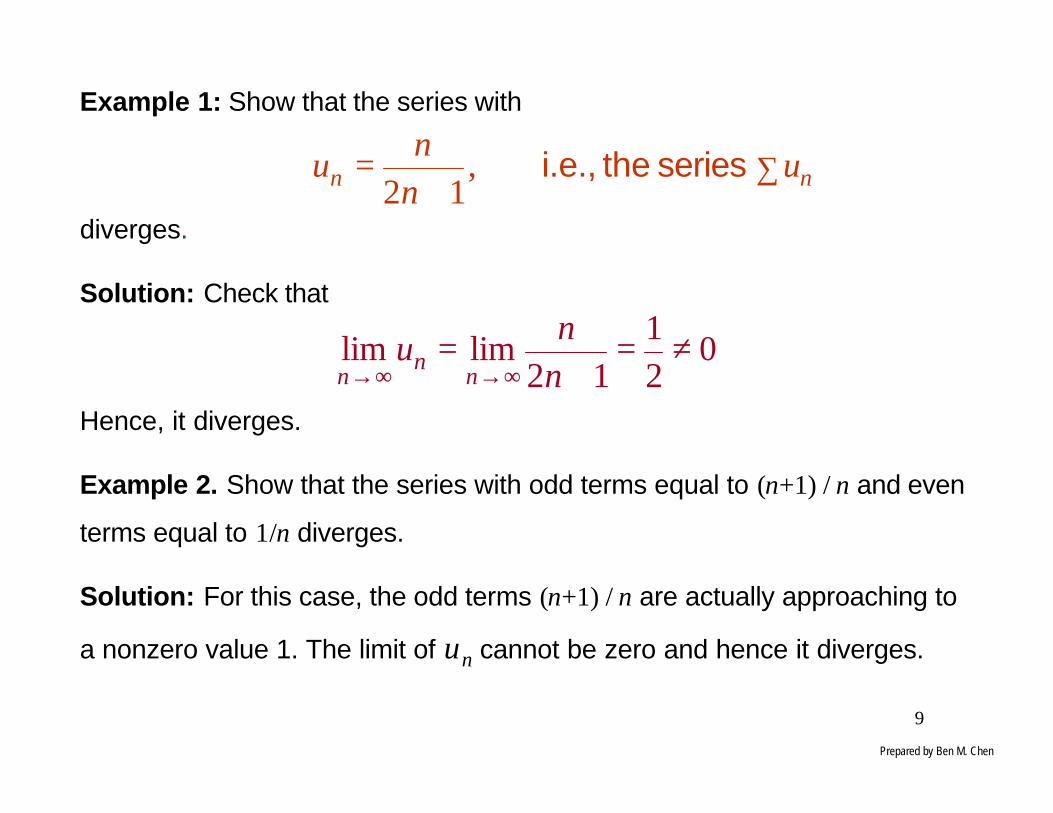
Example 1: Show that the series with

diverges.

Solution: Check that

Hence, it diverges.

Example 2. Show that the series with odd terms equal to (n+1) / n and even

terms equal to 1/n diverges.

Solution: For this case, the odd terms (n+1) / n are actually approaching to

a nonzero value 1. The limit of un cannot be zero and hence it diverges.

∑+

= nn unn

u ,12

series the i.e.,

021

12limlim ≠=

+=

∞→∞→ nn

un

nn


10

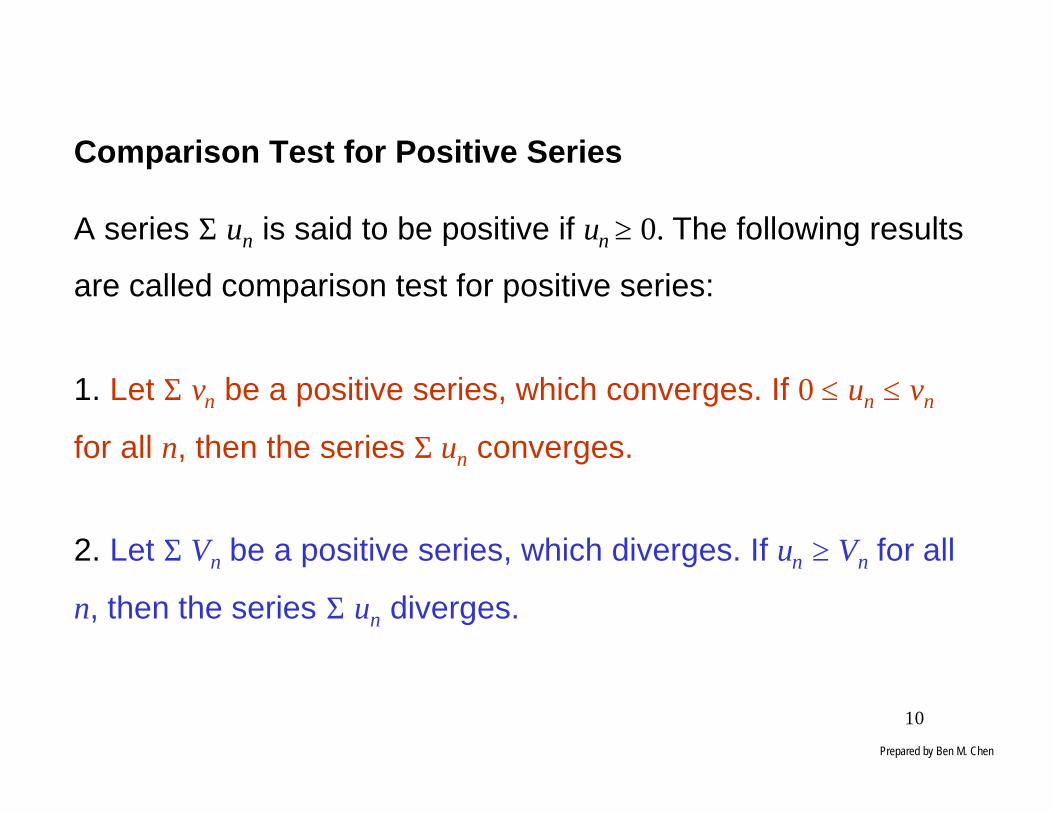
Comparison Test for Positive Series

A series Σ un is said to be positive if un ≥ 0. The following results

are called comparison test for positive series:

1. Let Σ vn be a positive series, which converges. If 0 ≤ un ≤ vn

for all n, then the series Σ un converges.

2. Let Σ Vn be a positive series, which diverges. If un ≥ Vn for all

n, then the series Σ un diverges.


11

Ratio Test for Positive Series

For positive series Σ un with

then

1. The series converges if T < 1.

2. The series diverges if T > 1.

3. No conclusion can be made if T = 1. Further test is needed.

Tu

u

n

n

n=+

∞→1lim

1

)!1(−

−=nn

nnuExample: Test the series with for convergence.

11

)/11(

1lim

)1(lim

)!1()1(

!limlim

11 <=

+=

+=

−⋅

+=

∞→∞→

−

∞→+

∞→ ennn

nn

nn

uu

nnn

n

n

n

nnn

n

n

Hence, it converges.Prepared by Ben M. Chen

12

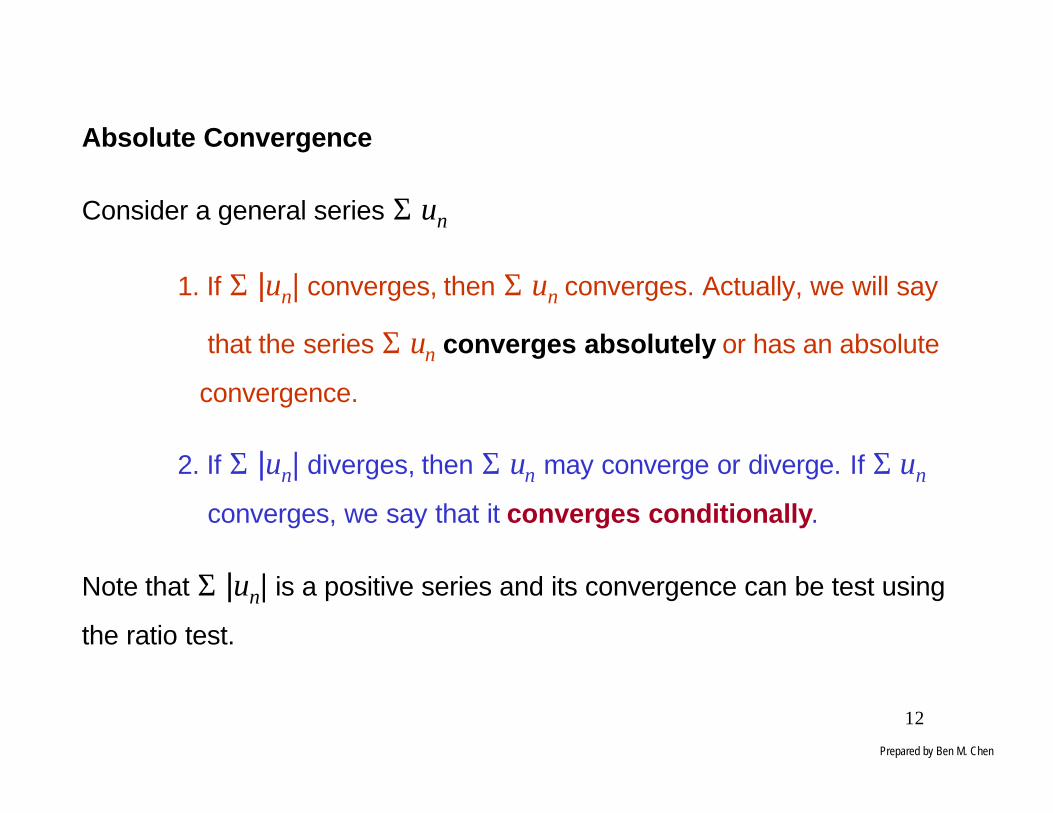
Absolute Convergence

Consider a general series Σ un

1. If Σ |un| converges, then Σ un converges. Actually, we will say

that the series Σ un converges absolutely or has an absolute

convergence.

2. If Σ |un| diverges, then Σ un may converge or diverge. If Σ un

converges, we say that it converges conditionally.

Note that Σ |un| is a positive series and its convergence can be test using

the ratio test.


13

Power Series

Any infinite series of the form

is called a power series, which can be written as a normal series,

LL +−++−+−+ nn axAaxAaxAA )()()( 2

210

∑∞

=−=

0)()( where)(

n

nnnn axAxuxu

Theorem (see lecture notes for proof): Consider the above power series. If

then the power series converges absolutely for any x such that

and the power series diverges for any x such that .

0lim 1 ≠=+∞→

LA

A

n

n

n

Lax

1<−

Lax

1>−


14

Example: Find the open interval of absolute convergence of the power series

LL +++++nxxx

xn

32

32

Solution: Using the theorem for power series, we have

Hence, the power series converges absolutely for all

and diverges for all

Ln

nA

Aa

nA

nn

n

nn ==

+=⇒==

∞→+

∞→1

1limlim0and

1 1

11or1 <<−< xx

1>x


15

Bessel′s Equation

The following second order differential equation,

is called Bessel′s equation of order v. Note that Bessel′s equation is a 2nd

order differential equation. It can be used to model quite a number of

problems in engineering such as the model of the displacement of a

suspended chain, the critical length of a vertical rod, and the skin effect

of a circular wire in AC circuits. The first application will be covered in

details in the class later on.

In general, it is very difficult to derive a closed-form solutions to differential

equations. As expected, the solution to the above Bessel′s equation cannot

be expressed in terms of some “nice” forms.

( ) 0222 =−+′+′′ yvxyxyx


16

Solution to Bessel′s Equation (Bessel Function of the First Kind)

The solution to the Bessel′s equation is normally expressed in terms of a power

series, which has a special name called Frobenius series. Such a method is

called Method of Frobenius. We define a power series (a Frobenius series),

where r and cn are free parameters. Without loss of any generality, let c0 ≠ 0.

Next, we will try to determine these parameters r and cn such that the above

Frobenius series is a solution of the Bessel′s equation, i.e., it will satisfy the

Bessel′s equation,

∑=∞

=

+

0)(

n

rnn xcxy

( ) 0222 =−+′+′′ yvxyxyx


17

Now, assume that the Frobenius series y(x) is indeed a solution to the

Bessel′s equation. We compute

Then, the Bessel′s equation gives

∑ +=′∞

=

−+

0

1)(n

rnn xrncy ∑ −++=′′

∞

=

−+

0

2)1)((n

rnn xrnrncy

( )

∑+∑−

∑ ++

∑ −++=

−+′+′′=

∞

=

++∞

=

+

∞

=

+

∞

=

+

0

2

0

2

0

0

222

)(

)1)((

0

n

rnn

n

rnn

n

rnn

n

rnn

xcxvc

xrnc

xrnrnc

yvxyxyx 22 −=⇒+= mnnm

Let

∑=

∑=∑

∞

=

+−

∞

=

+−

∞

=

++

22

22

0

2

n

rnn

m

rmm

n

rnn

xc

xcxc

20 =⇒= mn

∞=⇒∞= mn


18

Thus,

( )∑+∑−∑ ++∑ −++=

−+′+′′=∞

=

+−

∞

=

+∞

=

+∞

=

+

22

0

2

00

222

)()1)((

0

n

rnn

n

rnn

n

rnn

n

rnn xcxvcxrncxrnrnc

yvxyxyx

[ ] ( )[ ] 1221

220

22

22 1)()( +∞

=

+− −++−+∑ +−+= rr

n

rnnnn xvrcxvrcxcvcrnc

∑+∑−∑ +=∞

=

+−

∞

=

+∞

=

+

22

0

2

0

2)(n

rnn

n

rnn

n

rnn xcxvcxrnc

zero! toequal bemust tscoefficien theseAll

0)( 220 =− vrc ( ) 0]1[ 22

1 =−+ vrc 0)( 222 =+−+ −nnn cvcrnc


19

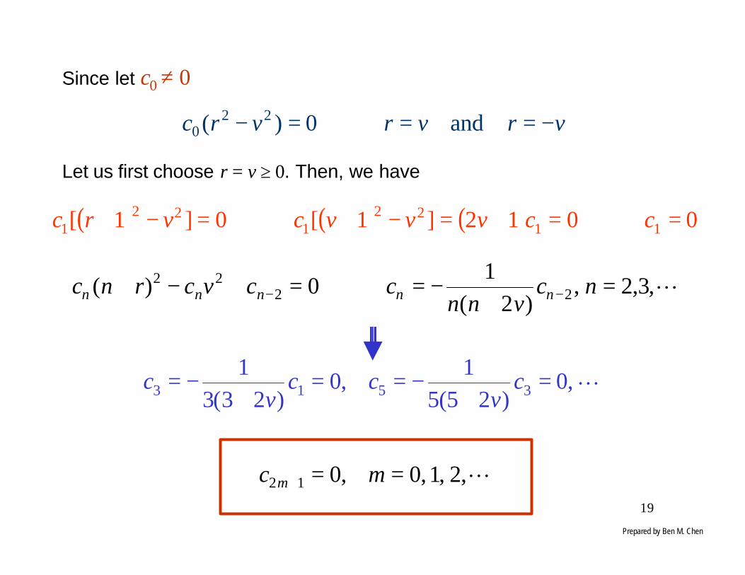
Since let c0 ≠ 0

Let us first choose r = v ≥ 0. Then, we have

vrvrvrc −==⇒=− and0)( 220

( ) ( ) ( ) 0012]1[0]1[ 1122

122

1 =⇒=+=−+⇒=−+ ccvvvcvrc

L,3,2,)2(

10)( 22

22 =+

−=⇒=+−+ −− ncvnn

ccvcrnc nnnnn

L,0)25(5

1,0

)23(3

13513 =

+−==

+−= c

vcc

vc

L,2,1,0,012 ==+ mc m


20

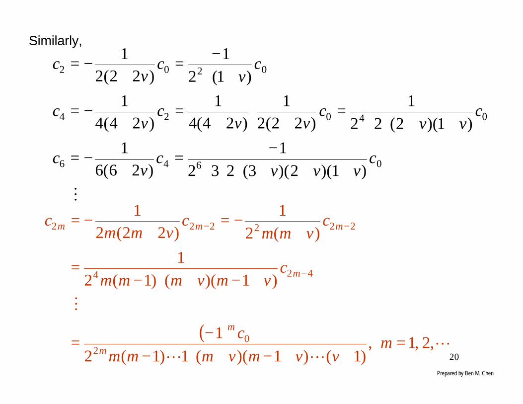
Similarly,

M

0646

04024

0202

)1)(2)(3(232

1)26(6

1

)1)(2(22

1)22(2

1)24(4

1)24(4

1

)1(2

1)22(2

1

cvvv

cv

c

cvv

cvv

cv

c

cv

cv

c

+++⋅⋅⋅−=

+−=

++⋅⋅=

+⋅

+=

+−=

+⋅−=

+−=

( )L

LL

M

,2,1,)1()1)((1)1(2

1

)1)(()1(2

1

)(2

1)22(2

1

20

424

222222

=++−+⋅−

−=

+−+⋅−=

+−=

+−=

−

−−

mvvmvmmm

c

cvmvmmm

cvmm

cvmm

c

m

m

m

mmm


21

Thus, we obtain a solution to the Bessel′s equation of order v,

( ) vm

mm

m

xvvmvmm

cxy +∞

=∑

++−+⋅−= 2

0201 )1()1)((!2

1)(

L

( )∑

++−+⋅−=

∞

=

+

02

2

01 )1()1)((!2

1)(

nn

vnn

vvnvnnx

cxyL

We need two linearly independent solutions to the Bessel′s equation in

order to characterized all its solutions as Bessel′s equation is a 2nd order

differential equation. We need to find another solution.

But, we will first introduce a Gamma function such that the above solution

to the Bessel′s equation y1(x) can be re-written in a neater way.


22

Gamma Function

For x > 0, we define a so-called Gamma function

If x > 0, then Γ(x+1) = x Γ(x).

For any positive integer n,

∫=Γ∞

−−

0

1)( dtetx tx

)(

)1(

0

1

0

1

0

00

xxdtetx

dtextet

detdtetx

tx

txtx

txtx

Γ==

+−=

−==+Γ

∫

∫

∫∫

∞−−

∞−−∞−

∞−

∞−

( ) !1!!!

)1(1)1()1()1()()1(

00

nnendten

nnnnnnnn

tt =⋅=−=∫=

Γ⋅−=−Γ−=Γ=+Γ∞−

∞−

L

0)1(

)1(

1,

lim

lim

lim

limlim1

=+−=

+−=

==

≤≤−=

−∞→

−

∞→

−

∞→

∞→

−

∞→

txkt

t

kx

t

t

x

t

t

x

t

tx

t

etkxx

etkxx

ext

kxket

et

L

L

L


23

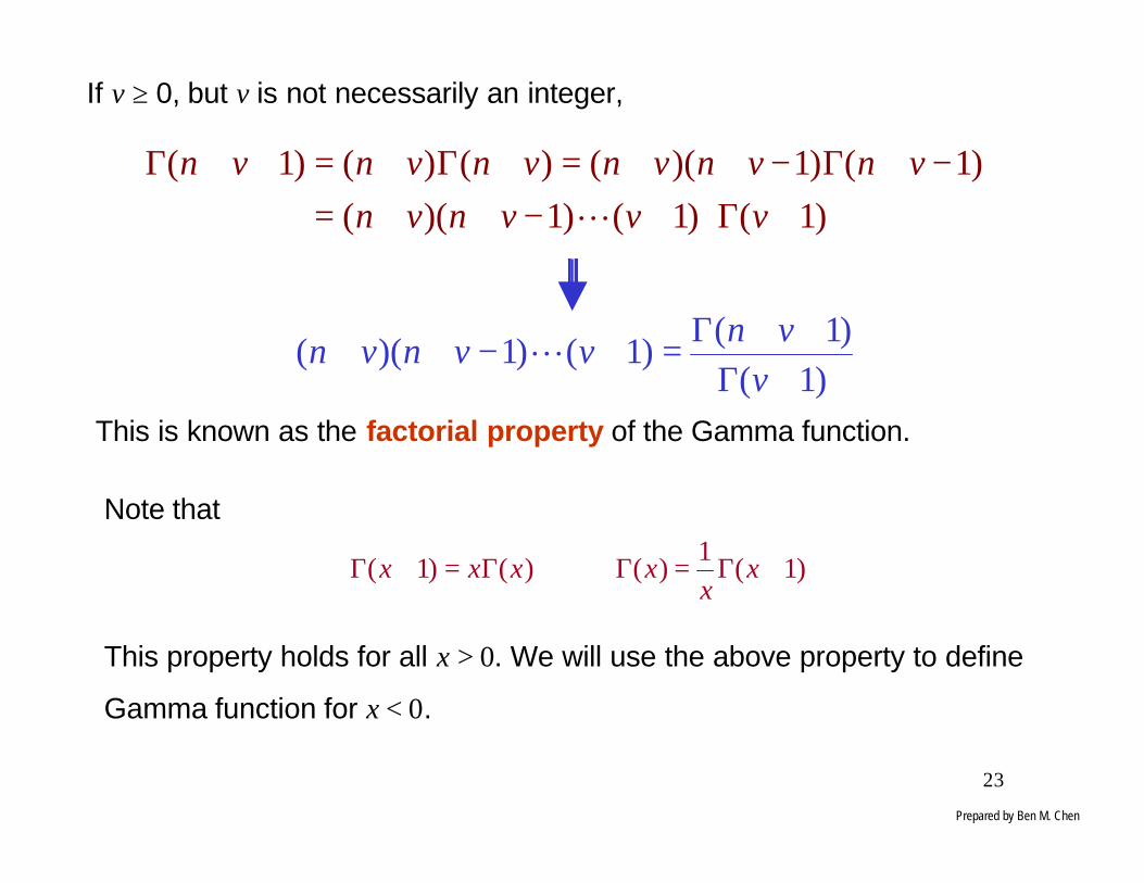
If v ≥ 0, but v is not necessarily an integer,

)1()1()1)((

)1()1)(()()()1(

+Γ⋅+−++=−+Γ−++=+Γ+=++Γ

vvvnvn

vnvnvnvnvnvn

L

)1(

)1()1()1)((

+Γ++Γ=+−++

vvn

vvnvn L

This is known as the factorial property of the Gamma function.

)1(1

)()()1( +Γ=Γ⇒Γ=+Γ xx

xxxx

Note that

This property holds for all x > 0. We will use the above property to define

Gamma function for x < 0.


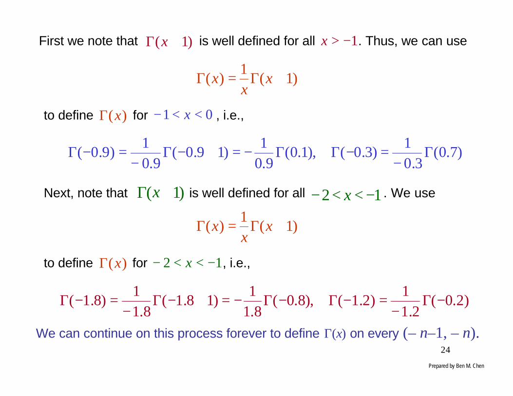
24

)1( +Γ xFirst we note that is well defined for all . Thus, we can use1−>x

)1(1

)( +Γ=Γ xx

x

to define for , i.e.,)(xΓ 01 <<− x

)7.0(3.0

1)3.0(),1.0(

9.01

)19.0(9.0

1)9.0( Γ

−=−ΓΓ−=+−Γ

−=−Γ

)1( +Γ xNext, note that is well defined for all . We use12 −<<− x

)1(1

)( +Γ=Γ xx

x

to define for , i.e.,)(xΓ 12 −<<− x

)2.0(2.1

1)2.1(),8.0(

8.11

)18.1(8.1

1)8.1( −Γ

−=−Γ−Γ−=+−Γ

−=−Γ

We can continue on this process forever to define Γ(x) on every (– n–1, – n).


25-4 -3 -2 -1 0 1 2 3 4

-20

-15

-10

-5

0

5

10

15

20

The Gamma Function

The Gamma function


26

Solution of Bessel′′s Equation in terms of Gamma Function

Recall that the first solution we have obtained for the Bessel′s equation, i.e.,

( )( )( ) ( )

( ) ( )( )

∑ ↵++Γ⋅⋅

+Γ−=

∑+⋅⋅⋅−++⋅⋅

−=

∞

=

+

∞

=

+

02

2

0

02

2

01

property factorial1!2

11

11!2

1)(

nn

vnn

nn

vnn

vnn

xvc

vvnvnn

xcxy

( )( ) ( ) ( )( )1

111

+Γ++Γ=+⋅⋅⋅−++

vvn

vvnvnLet us choose

( )12

10 +Γ

=v

c v ( ) ( ) ( )( )∑

∞

=+

+

++Γ⋅⋅−

==0

2

2

1 1!2

1

nvn

vnn

v vnnx

xJxy

Jv(x) is called a Bessel Function of the 1st kind of order v. This power series

converges for all positive x (prove it yourself).Prepared by Ben M. Chen

27

Exercise Problem: Verify that

( ) ( ) ( )[ ]xJxJxJ vvv 112

1+− −=′

Solution:

( ) ( )( )

( ) ( )( )

( ) ( )( )

( )( )( )∑∑

∑

∑

∞

=+

−+∞

=−+

−+

−

∞

=+

−+

∞

=+

+

++Γ−+=

+Γ−=

⇓

++Γ−+=

⇓

++Γ−=

02

12

012

12

1

02

12

02

2

1!2

12

!2

1x

1!2

1)2('

1!2

1

nvn

vnn

nvn

vnn

v

nvn

vnn

v

nvn

vnn

v

vnnxvn

vnnx

J

vnnxvn

xJ

vnnx

xJ

Γ(n+v+1) = (n+v) Γ(n+v)

( ) ( )xJxJ vv 121

−−′


28

( ) ( ) ( )( )

( )( ) ( )

( )( )

( )( )

( )xJ

vnnx

vnnx

vnnx

vnnxn

xJxJ

v

nvn

vnn

nvn

vnn

nvn

vnn

nvn

vnn

vv

1

012

12

022

121

12

12

02

12

1

2

1

2!2

1

2

1

2!2

1

1!12

10

1!2

1

2

1'

+

∞

=++

++

∞

=++

+++

∞

=+

−+

∞

=+

−+

−

−=

++Γ−

−=

++Γ−=

++Γ−−+=

++Γ−=−

∑

∑

∑

∑

n := n – 1

( ) ( ) ( )[ ]xJxJxJ vvv 112

1' +− −=


29

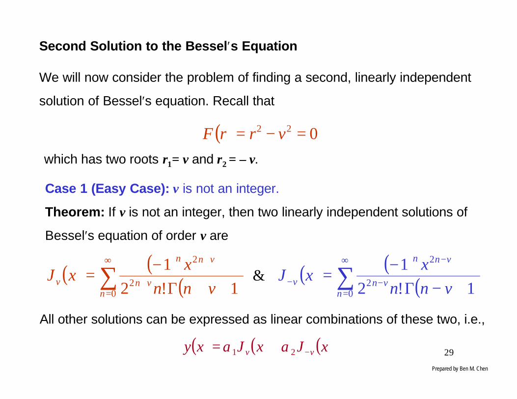
Second Solution to the Bessel′s Equation

We will now consider the problem of finding a second, linearly independent

solution of Bessel′s equation. Recall that

( ) 022 =−= vrrF

which has two roots r1= v and r2 = – v.

Case 1 (Easy Case): v is not an integer.

Theorem: If v is not an integer, then two linearly independent solutions of

Bessel′s equation of order v are

( ) ( )( )∑

∞

=+

+

++Γ−=

02

2

1!2

1

nvn

vnn

v vnnx

xJ ( ) ( )( )∑

∞

=−

−

− +−Γ−=

02

2

1!2

1

nvn

vnn

v vnnx

xJ&

All other solutions can be expressed as linear combinations of these two, i.e.,

( ) ( ) ( )xJxJxy vv −+= 21 ααPrepared by Ben M. Chen

30

Case 2 (Complicated Case): v is a nonnegative integer

If v is a nonnegative integer, say v = k. In this case, Jv(x) and J–v(x) are

solutions of Bessel′s equation of order v, but they are NOT linearly

independent. This fact can be verified from the following arguments: First

note that

( ) ( )( )∑

∞

=−

−

− +−Γ−=

02

2

1!2

1

nkn

knn

k knnx

xJ

Observing the values of Gamma function at 0, –1, – 2, ..., they go to infinity.

Thus we have

( ) ( ) 01

1or 1 →

+−Γ∞→+−Γ

knkn

for n – k + 1 = 0, – 1, – 2, …, or n = k – 1, k – 2, k – 3, …, 0


31

-4 -3 -2 -1 0 1 2 3 4-20

-15

-10

-5

0

5

10

15

20

The Gamma Function

The Gamma function


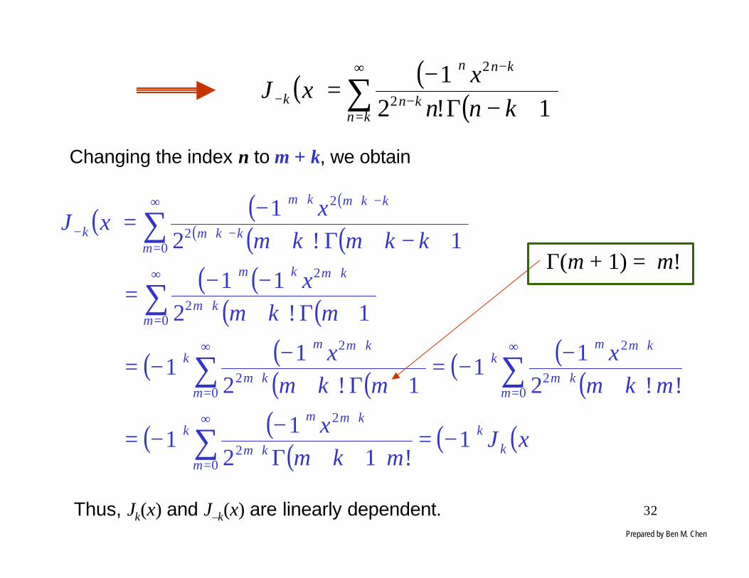
32

( ) ( )( )∑

∞

=−

−

− +−Γ−=

knkn

knn

k knnx

xJ1!2

12

2

( ) ( ) ( )

( ) ( ) ( )( ) ( )

( ) ( )

( ) ( )( ) ( ) ( ) ( )

( )

( ) ( )( ) ( ) ( )xJ

mkmx

mkmx

mkmx

mkmx

kkmkmx

xJ

kk

mkm

kmmk

mkm

kmmk

mkm

kmmk

mkm

kmkm

mkkm

kkmkm

k

1!12

11

!!2

11

1!2

11

1!2

11

1!2

1

02

2

02

2

02

2

02

2

02

2

−=++Γ

−−=

+−−=

+Γ+−−=

+Γ+−−=

+−+Γ+−=

∑

∑∑

∑

∑

∞

=+

+

∞

=+

+∞

=+

+

∞

=+

+

∞

=−+

−++

−

Changing the index n to m + k, we obtain

Thus, Jk(x) and J–k(x) are linearly dependent.

Γ(m + 1) = m!


33

Summary of results obtained so far:

We deal with Bessel′s equation in this topic,

We have shown that it has a solution,

If v is not an integer, we have Jv(x) and J–v(x) being linearly independent.

Hence, all its solution can be expressed as,

( ) 0,0''' 222 ≥=−++ vyvxxyyx

( ) ( )( )∑

∞

=+

+

++Γ−=

02

2

1!2

1

nvn

vnn

v vnnx

xJ

( ) ( ) ( )xJxJxy vv −+= 21 αα

If v is an integer, Jv(x) and J–v(x) are linearly dependent and we need to

search for a new solution …….Prepared by Ben M. Chen

34

A 2nd Solution to Bessel′′s Equation for Case v = k = 0

Let us try a solution of the following format (why? Only God knows.)

( ) ( ) ( ) n

nn xcxxyxy ∑

∞

=

+=1

*12 ln ( ) ( ) ( )

( )∑∞

=

−==0

22

2

01!2

1

nn

nn

nx

xJxywhere

( ) ( ) ( ) ( ) 1

1

*002

1ln'' −

∞

=∑++= n

nn xncxJ

xxxJxy

( ) ( ) ( ) ( ) ( ) ( )∑∞

=

−−+−+=1

2*02002 1

1'

2ln''''

n

nn xcnnxJ

xxJ

xxxJxy

If y2(x) is a solution to the Bessel′s equation of order 0, it must satisfy its

differential equation….


35

Substituting the above equations into Bessel′s equation of order 0, i.e.,

( ) 0'''0''' 222 =++=−++ xyyxyyxxyyx

( ) ( ) ( ) ( ) ( )

( ) ( ) ( )

( ) ( ) ∑

∑

∑

∞

=

+

∞

=

−

∞

=

−

++

+++

−+−+=

1

1*0

1

1*00

1

1*000

ln

1ln'

11

'2ln''0

n

nn

n

nn

n

nn

xcxxJx

xncxJx

xxJ

xcnnxJx

xJxxJx

( ) ( ) ( ) ( )[ ]xJxxJxJxx 000 '''ln0 ++=

1*

1

2 −∞

=∑ n

nn

xcn

( ) 0'21

1*

1

1*20 =++ ∑∑

∞

=

+∞

=

−

n

nn

n

nn xcxcnxJ


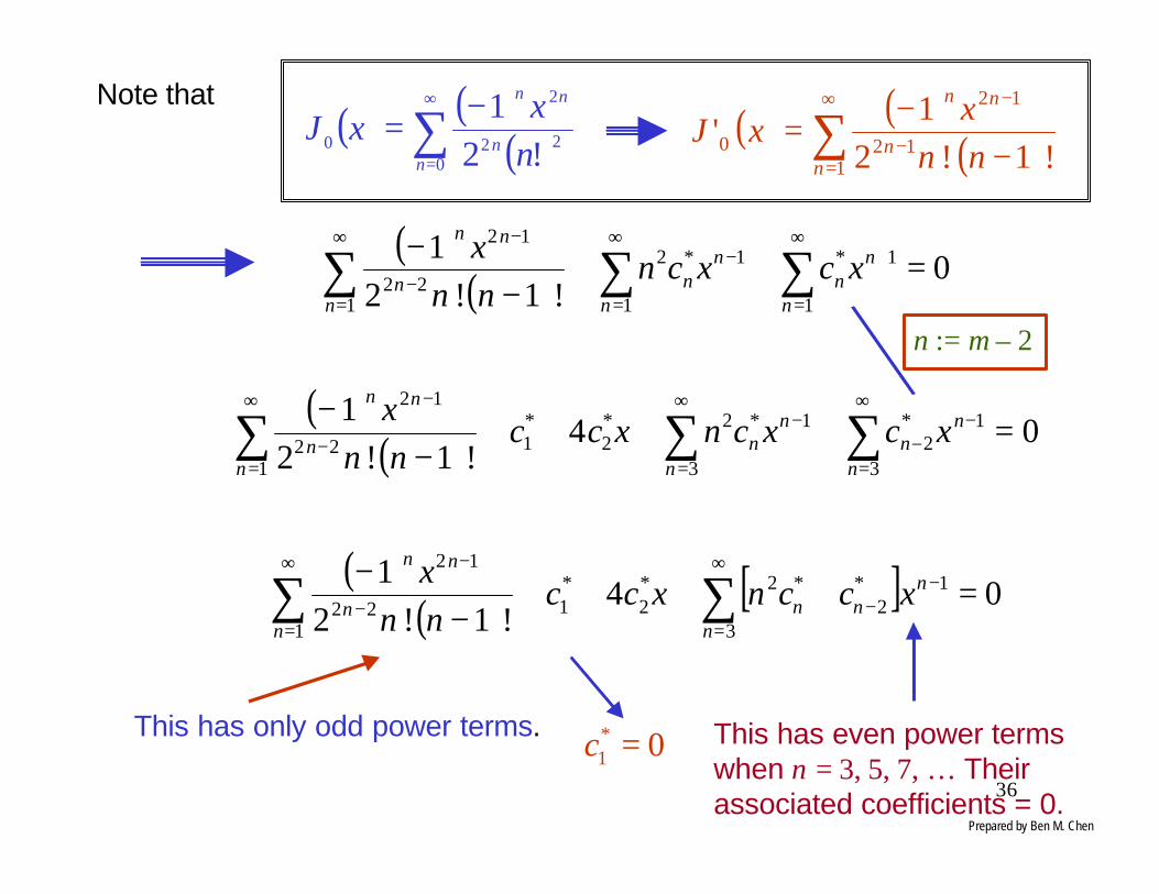
36

( ) ( )( )∑

∞

=−

−

−−

=1

12

12

0 !1!2

1'

nn

nn

nnx

xJNote that

( )( )

( )( )

( )( ) [ ] 04

!1!2

1

04!1!2

1

0!1!2

1

3

1*2

*2*2

*1

122

12

3

1*2

3

1*2*2

*1

122

12

1

1*

1

1*2

122

12

=++++−

−

⇓

=++++−

−

⇓

=++−

−

∑∑

∑∑∑

∑∑∑

∞

=

−−

∞

=−

−

∞

=

−−

∞

=

−∞

=−

−

∞

=

+∞

=

−∞

=−

−

n

nnn

nn

nn

n

nn

n

nn

nn

nn

n

nn

n

nn

nn

nn

xccnxccnnx

xcxcnxccnnx

xcxcnnnx

n := m – 2

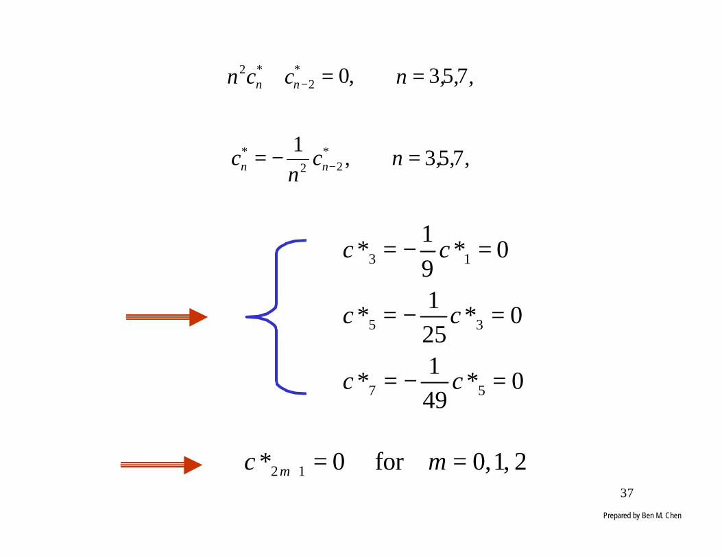
This has only odd power terms.0*

1 =c This has even power terms when n = 3, 5, 7, … Their associated coefficients = 0.

( ) ( )( )∑

∞

=

−=0

22

2

0 !21

nn

nn

nx

xJ


37

⋅⋅⋅=−=

⇓

⋅⋅⋅==+

−

−

,,,ncn

c

,,,nccn

nn

nn

753 ,1

753 ,0

*22

*

*2

*2

⋅⋅⋅=−=

=−=

=−=

0*49

1*

0*25

1*

0*9

1*

57

35

13

cc

cc

cc

⋅⋅⋅==+ 2 ,1 ,0for 0* 12 mc m


38

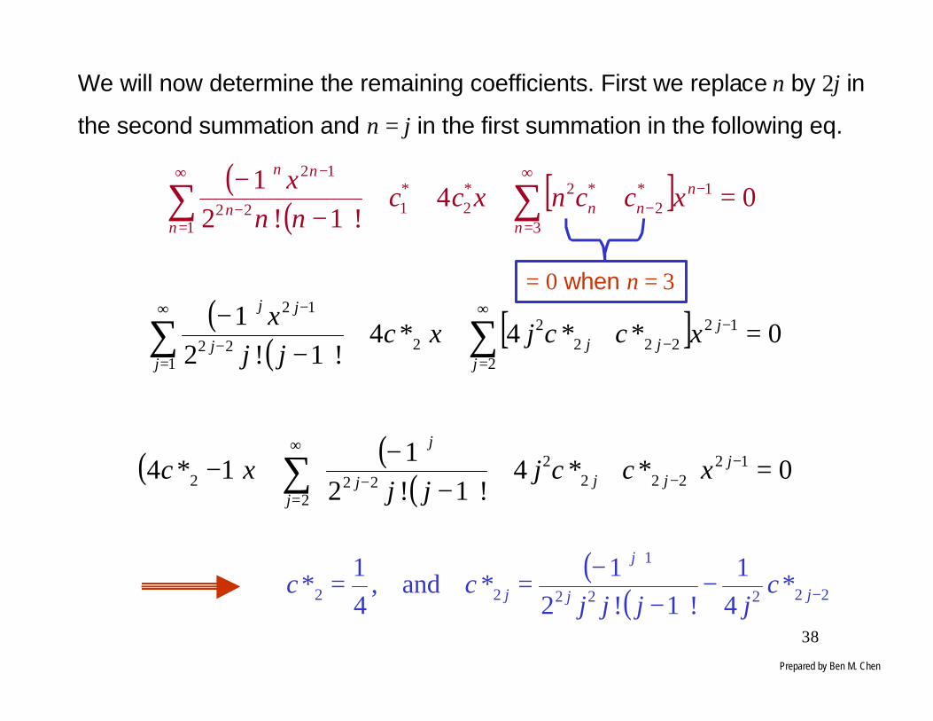
We will now determine the remaining coefficients. First we replace n by 2j in

the second summation and n = j in the first summation in the following eq.

( )( ) [ ] 04

!1!2

1

3

1*2

*2*2

*1

122

12

=++++−

− ∑∑∞

=

−−

∞

=−

−

n

nnn

nn

nn

xccnxccnnx

( )( ) [ ]

( ) ( )( ) 0**4

!1!2

11*4

0**4*4!1!2

1

12

2222

2222

1 2

12222

2222

12

=

++

−−

+−

⇓

=+++−

−

⇓

−∞

=−−

∞

=

∞

=

−−−

−

∑

∑ ∑

j

jjjj

j

j j

jjjj

jj

xccjjj

xc

xccjxcjj

x

( )( ) 22222

1

22 *4

1

!1!2

1*and,

4

1* −

+

−−

−== jj

j

j cjjjj

cc

= 0 when n = 3


39

+−=−−=

2

11

42

1

422

1

222

1* 2222244c

++=

⋅

++

⋅=

3

1

2

11

642

1

423421

1

2632

1* 222222266c

( )( )

( )( ) ( )jjjj

cj

jj

j ψ22

1

222

1

2!2

11

3

1

2

11

242

1*

++ −=

+⋅⋅⋅+++

⋅⋅⋅−

=

( )j

j1

3

1

2

11 +⋅⋅⋅+++=ψ


40

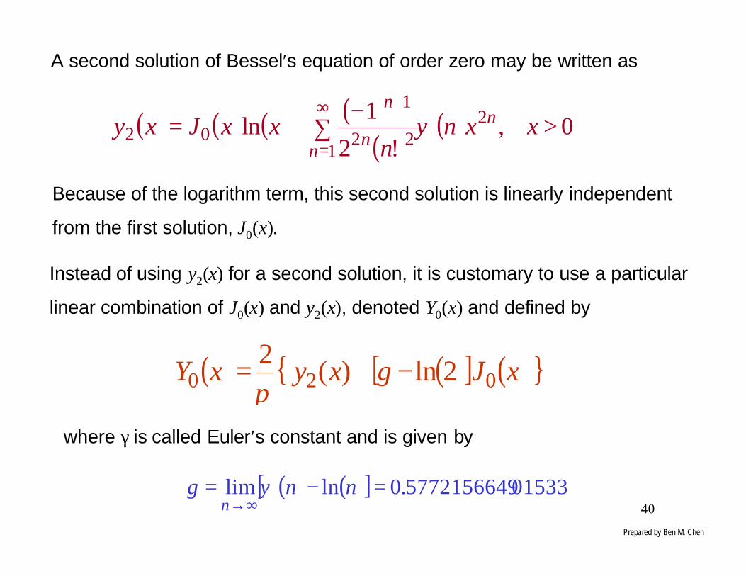
A second solution of Bessel′s equation of order zero may be written as

( ) ( ) ( ) ( )( )

( ) 0,!2

1ln

1

222

1

02 >∑−+=

∞

=

+xxn

nxxJxy

n

nn

n

ψ

Because of the logarithm term, this second solution is linearly independent

from the first solution, J0(x).

( ) ( )[ ] ( ){ }xJxyxY 020 2ln)(2 −+= γπ

where γ is called Euler′s constant and is given by

( ) ( )[ ] ⋅⋅⋅=−=∞→

015335772156649.0lnlim nnn

ψγ

Instead of using y2(x) for a second solution, it is customary to use a particular

linear combination of J0(x) and y2(x), denoted Y0(x) and defined by


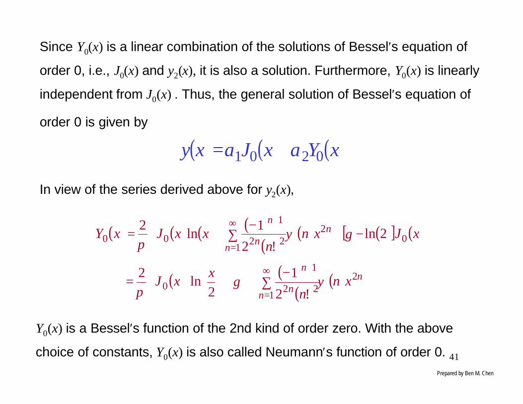
41

Since Y0(x) is a linear combination of the solutions of Bessel′s equation of

order 0, i.e., J0(x) and y2(x), it is also a solution. Furthermore, Y0(x) is linearly

independent from J0(x) . Thus, the general solution of Bessel′s equation of

order 0 is given by

( ) ( ) ( )xYxJxy 0201 αα +=

In view of the series derived above for y2(x),

( ) ( ) ( ) ( )( )

( ) ( )[ ] ( )

( ) ( )( )

( )

∑−

+

+

=

−∑ +−

+=

∞

=

+

∞

=

+

n

nn

n

n

nn

n

xnn

xxJ

xJxnn

xxJxY

2

122

1

0

01

222

1

00

!2

1

2ln

2

2ln!2

1ln

2

ψγπ

γψπ

Y0(x) is a Bessel′s function of the 2nd kind of order zero. With the above

choice of constants, Y0(x) is also called Neumann′s function of order 0.Prepared by Ben M. Chen

42

A 2nd Solution of Bessel′s Equation of Order v (positive integer).

If v is a positive integer, say v = k, then a similar procedure as in the k = 0

case, but more involved calculation leads us to the following 2nd solution

of Bessel′s equation of order v = k,

( ) ( ) ( ) ( ) ( ) ( )[ ]( )

∑+

++−+∑−−−

+

=

∞

=

+++

+−

=

−+−

0

212

11

0

212 !!2

1

!2

!12

ln2

n

knkn

nk

n

knknkk x

knn

knnx

n

nkxxJxY

ψψγ

π

Yk(x) and Jk(x) are linearly independent for x > 0, and the general solution of

Bessel′s equation of order k is given by

( ) ( ) ( )xYxJxy kk 21 αα +=

Although Jk(x) is simple Jv(x) for the case v = k, our derivation of Yk(x) does

not suggest how Yv(x) might be defined if v is not a nonnegative integer.


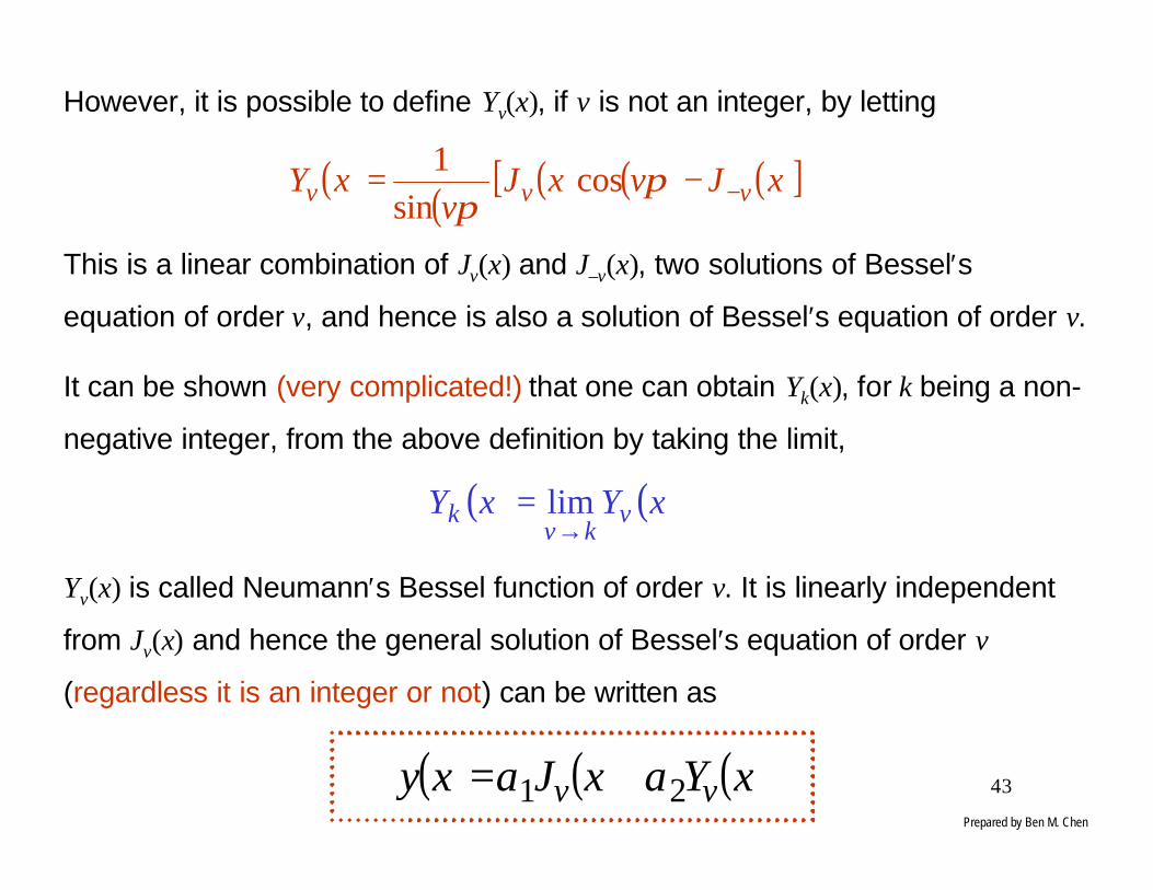
43

However, it is possible to define Yv(x), if v is not an integer, by letting

( ) ( ) ( ) ( ) ( )[ ]xJvxJv

xY vvv −−= ππ

cossin

1

This is a linear combination of Jv(x) and J–v(x), two solutions of Bessel′s

equation of order v, and hence is also a solution of Bessel′s equation of order v.

It can be shown (very complicated!) that one can obtain Yk(x), for k being a non-

negative integer, from the above definition by taking the limit,

( ) ( )xYxY vkv

k→

= lim

Yv(x) is called Neumann′s Bessel function of order v. It is linearly independent

from Jv(x) and hence the general solution of Bessel′s equation of order v

(regardless it is an integer or not) can be written as

( ) ( ) ( )xYxJxy vv 21 αα +=Prepared by Ben M. Chen

44

Extra: Linear Dependence and Linear IndependenceExtra: Linear Dependence and Linear Independence

Given two functions f (x) and g(x), they are said to be linearly independent if

and only if

holds with a = 0 and b = 0. Otherwise, they are said to be dependent, i.e.,

there exist either nonzero a and/or nonzero b such that

Assume that a is nonzero. We can then rewrite the above equation as

f (x) and g(x) are related by a constant and hence they are dependent to one

another.

defined allfor 0)()( xxgbxfa =⋅+⋅

defined. allfor 0)()( xxgbxfa =⋅+⋅

( ) )()()( xgxgabxf ⋅=⋅−= α


45

Now, given Jv(x) and J-v(x) are linearly independent, show that Jv(x) and Yv(x) with

are also linearly independent.

Proof. Rewrite Yv(x) as

and let

Hence, Jv(x) and Yv(x) are linearly independent.

( )( )

( ) ( ) ( )[ ]xJvxJv

xY vvv −−= ππ

cossin

1

( ) ( ) ( ) ( ) ( )[ ] ( ) ( ) 0,cossin

1≠+=−= −− ββαπ

πxJxJxJvxJ

vxY vvvvv

[ ] 0)()()(0)()( =++⇒=⋅+⋅ − xJxJbxJaxYbxJa vvvvv βα

0)()()( =++⇒ − xJbxJba vv βα

0,00,0)( ==⇒==+⇒ abbba βα


46

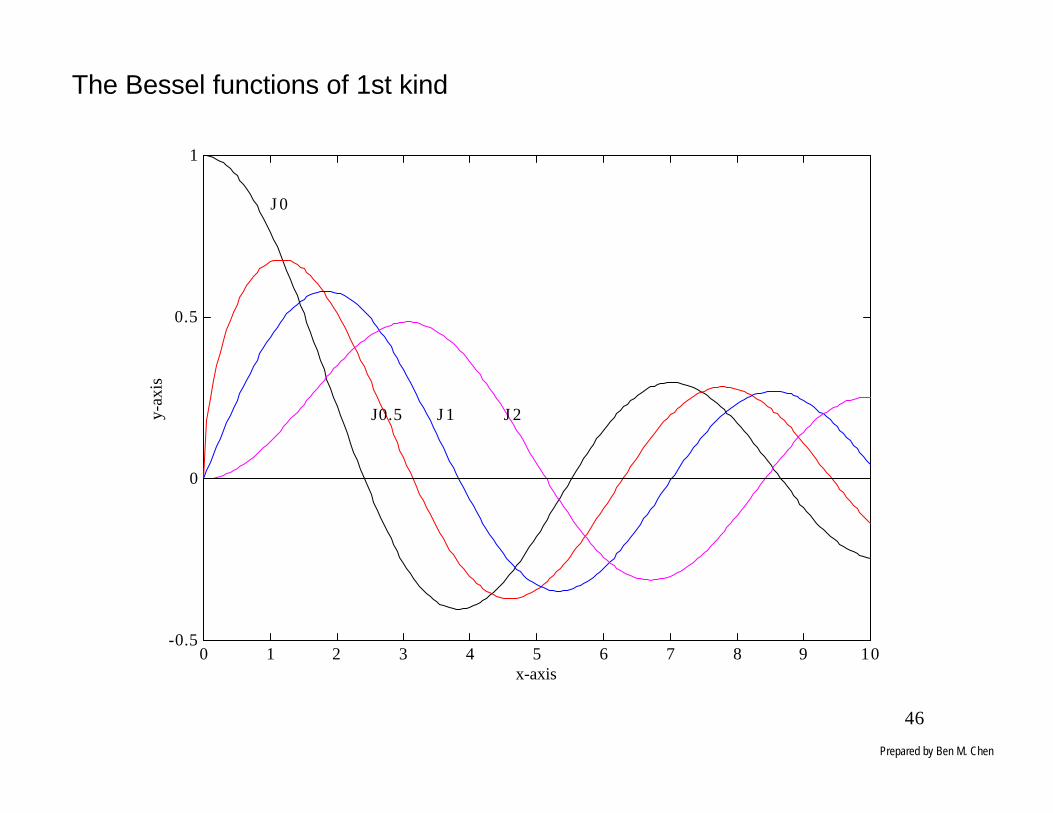
0 1 2 3 4 5 6 7 8 9 10-0.5

0

0.5

1

J 0

J0.5 J 1 J 2

x-axis

y-ax

is

The Bessel functions of 1st kind


47

Bessel functions of the 2nd kind

0 1 2 3 4 5 6 7 8 9 10-3

-2.5

-2

-1.5

-1

-0.5

0

0.5

1

Key observation: All these function start from negative infinity

Y0 Y0.5

Y1Y2

x-axis

y-ax

is


48

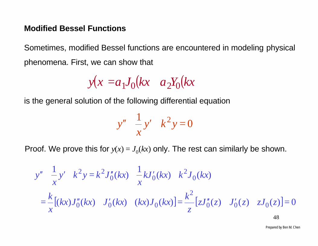
Modified Bessel Functions

Sometimes, modified Bessel functions are encountered in modeling physical

phenomena. First, we can show that

is the general solution of the following differential equation

( ) ( ) ( )kxYkxJxy 0201 αα +=

01 2 =+′+′′ ykyx

y

Proof. We prove this for y(x) = J0(kx) only. The rest can similarly be shown.

[ ] [ ] 0)()()()()()()()(

)()(1

)(1

000

2

000

02

0022

=+′+′′=+′+′′=

+′+′′=+′+′′

zzJzJzJzz

kkxJkxkxJkxJkx

xk

kxJkkxJkx

kxJkykyx

y


49

Now, let k = i, where i = , which implies k2 = i2 = –1. Then

is the general solution of

which is called a modified Bessel′s equation of order 0, and J0(ix) is a

modified Bessel function of the first kind of order 0. Usually, we denote

1−

( ) ( ) ( )ixYixJxy 0201 αα +=

01 =−′+′′ yyx

y

( ) ( )ixJxI 00 =

Since i2 = −1, substitution of ix for x in the series for J0 yields:

It is a real function of x.

( ) ⋅⋅⋅++++= 6222

422

220

642

1

42

1

2

11 xxxxI

( ) ( )( )∑

∞

=

−=0

22

2

0 !21

nn

nn

nx

xJPrepared by Ben M. Chen

50

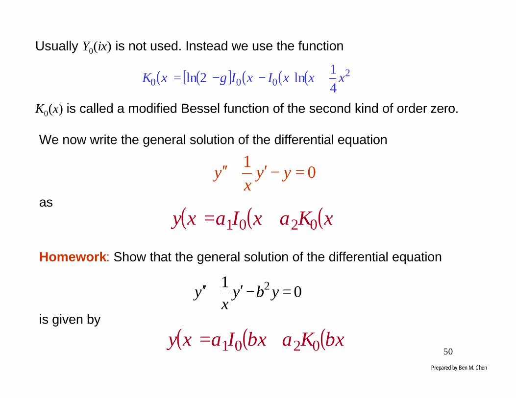
Usually Y0(ix) is not used. Instead we use the function

K0(x) is called a modified Bessel function of the second kind of order zero.

( ) ( )[ ] ( ) ( ) ( ) ⋅⋅⋅++−−= 2000 4

1ln2ln xxxIxIxK γ

We now write the general solution of the differential equation

as

Homework: Show that the general solution of the differential equation

is given by

01 =−′+′′ yyx

y

( ) ( ) ( )xKxIxy 0201 αα +=

01 2 =−′+′′ ybyx

y

( ) ( ) ( )bxKbxIxy 0201 αα +=Prepared by Ben M. Chen

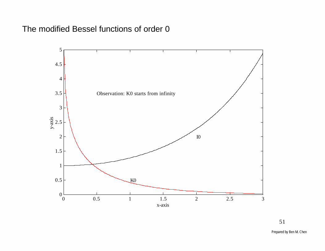
51

0 0.5 1 1.5 2 2.5 30

0.5

1

1.5

2

2.5

3

3.5

4

4.5

5

x-axis

y-ax

is

I0

K0

Observation: K0 starts from infinity

The modified Bessel functions of order 0


52

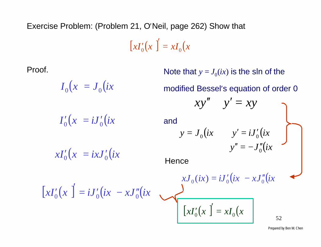
Exercise Problem: (Problem 21, O′Neil, page 262) Show that

Proof.

( )[ ] ( )xxIxIx 00 =′′

( ) ( )

( ) ( )

( ) ( )

( )[ ] ( ) ( )ixJxixJixIx

ixJixxIx

ixJixI

ixJxI

000

00

00

00

′′−′=′′

⇓

′=′⇓

′=′⇓

=Note that y = J0(ix) is the sln of the

modified Bessel′s equation of order 0

and

xyyyx =′+′′

( ) ( )( )ixJy

ixJiyixJy

0

00

′′−=′′⇒

′=′⇒=

Hence

( ) ( )ixJxixJiixxJ 000 )( ′′−′=

( )[ ] ( )xxIxIx 00 =′′


53

Applications of Bessel Functions (Oscillations of a Suspended Chain)

Displacement of a Suspended Chain

Suppose we have a heavy flexible chain. The chain is fixed at the upper

end and free at the bottom.

We want to describe the oscillations caused by a small displacement in a

horizontal direction from the stable equilibrium position.

x y


54

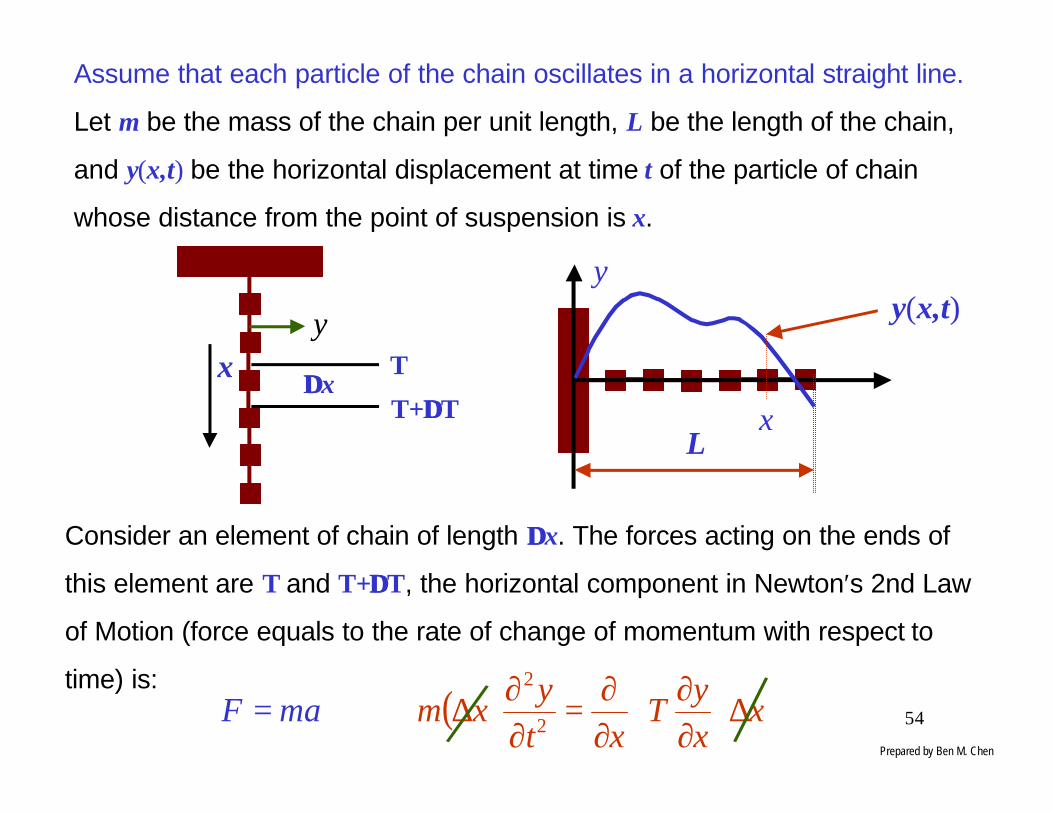
Assume that each particle of the chain oscillates in a horizontal straight line.

Let m be the mass of the chain per unit length, L be the length of the chain,

and y(x,t) be the horizontal displacement at time t of the particle of chain

whose distance from the point of suspension is x.

Consider an element of chain of length ∆∆x. The forces acting on the ends of

this element are T and T+∆∆T, the horizontal component in Newton′s 2nd Law

of Motion (force equals to the rate of change of momentum with respect to

time) is:

yy(x,t)

xL

y

∆∆xT

T+∆∆T

( ) xxy

Txt

yxm ∆

∂∂

∂∂=

∂∂∆ 2

2

⇒= maF

x


55

∂∂

∂∂=

∂∂

xy

Txt

ym 2

2

( ) acts ebelow wher chain theof weight theis where TxLmgT −=

( )

∂∂−+

∂∂−=

∂∂−

∂∂−

∂∂=

∂∂

∂∂

−∂∂

=

∂∂

−∂∂

∂∂

=∂∂

2

2

2

2

2

2

2

2

2

2

xy

xLgxy

gmxy

mgx

ymgx

xy

mgL

xy

xx

mgx

ymgL

xy

mgxxy

mgLxt

ym

( )2

2

2

2

xy

xLgxy

gty

∂∂

−+∂∂

−=∂∂

This is a partial differential equation. However, we can reduce it to a problem

involving only an ordinary differential equation. Prepared by Ben M. Chen

56

Let z = L − x and u(z, t) = y (L − z, t). Then

2

2

2

2

2

2

2

2

xy

zx

xy

xxy

zzu

zzu

zu

xz

zu

xu

xy

tu

ty

∂∂=

∂∂

∂∂

∂∂−=

∂∂

∂∂−=

∂∂

∂∂=

∂∂

∂∂−=

∂∂⋅

∂∂=

∂∂=

∂∂

∂∂=

∂∂

2

2

2

2

zu

gzzu

gtu

∂∂+

∂∂=

∂∂⇒( )

2

2

2

2

xy

xLgxy

gty

∂∂

−+∂∂

−=∂∂

This is still a partial differential equation, which can be solved using p.d.e.

method. Since we anticipate the oscillations to be periodic in t, we will

attempt a solution of the form ( ) ( ) ( )θω −= tzftzu cos,

( ) ( ) ( ) ( ) ( ) ( )θωθωθωω −′′+−′=−− tzfgztzfgtzf coscoscos2


57

Dividing the above equation by , we get a differential equation( )δω −tgz cos

( ) ( ) ( ) 01 2

=+′+′′ zfgz

zfz

zfω

It is shown in the lecture notes that and are the

solutions of

( )cn

a bxJx ( )cn

a bxYx

012

2

2222222 =

−++′

−

−′′ − yx

cnaxcby

xa

y c

0 0

g

2

21

122

0 112

222

222

=⇒=−

=⇒=

=⇒−=−

=⇒−=−

ncna

bg

cb

cc

aa

ωω

We let

Thus, the general solution is in terms

of Bessel functions of order zero:

( )

+

=

gz

Ygz

Jzf ωαωα 22 0201


58

0 1 2 3 4 5 6 7 8 9 10-3

-2.5

-2

-1.5

-1

-0.5

0

0.5

1

Key observation: All these function start from negative infinity

Y0 Y0.5

Y1Y2

x-axis

y-ax

is

Bessel functions of the 2nd kind


59

Lxzgz

Y →→−∞→

or0 as,20 ω

We must therefore choose α2 = 0 in order to have a bounded solution, as

expected from the physical setting of the problem. This leaves us with

( )

=

gz

Jzf ωα 201

Thus,

and hence

( ) ( ) ( ) ( )θωωαθω −

=−= t

gz

Jtzftzu cos2cos, 01

( ) ( )θωωα −

−= tg

xLJtxy cos2, 01


60

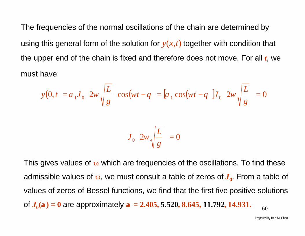
The frequencies of the normal oscillations of the chain are determined by

using this general form of the solution for y(x,t) together with condition that

the upper end of the chain is fixed and therefore does not move. For all t, we

must have

( ) ( ) ( )[ ]

02

02coscos2,0

0

0101

=

⇓

=

−=−

=

gL

J

gL

JttgL

Jty

ω

ωθωαθωωα

This gives values of ω which are frequencies of the oscillations. To find these

admissible values of ω, we must consult a table of zeros of J0. From a table of

values of zeros of Bessel functions, we find that the first five positive solutions

of J0(αα) = 0 are approximately αα = 2.405, 5.520, 8.645, 11.792, 14.931.


61

0 1 2 3 4 5 6 7 8 9 10-0.5

0

0.5

1

J 0

J0.5 J 1 J 2

x-axis

y-ax

is

The Bessel functions of 1st kind

2.405 5.5208.645


62

Using the these zeros, we obtain

Lg

gL

Lg

gL

Lg

gL

Lg

gL

Lg

gL

466.7 931.142

896.5 792.112

327.4 645.82

760.2 520.52

203.1 405.22

55

44

33

22

11

=⇒=

=⇒=

=⇒=

=⇒=

=⇒=

ωω

ωω

ωω

ωω

ωω

All these are admissible values of ω, and they represent frequencies of the

normal modes of oscillation. The period Tj associated with ωj is

jjT

ωπ2=


63

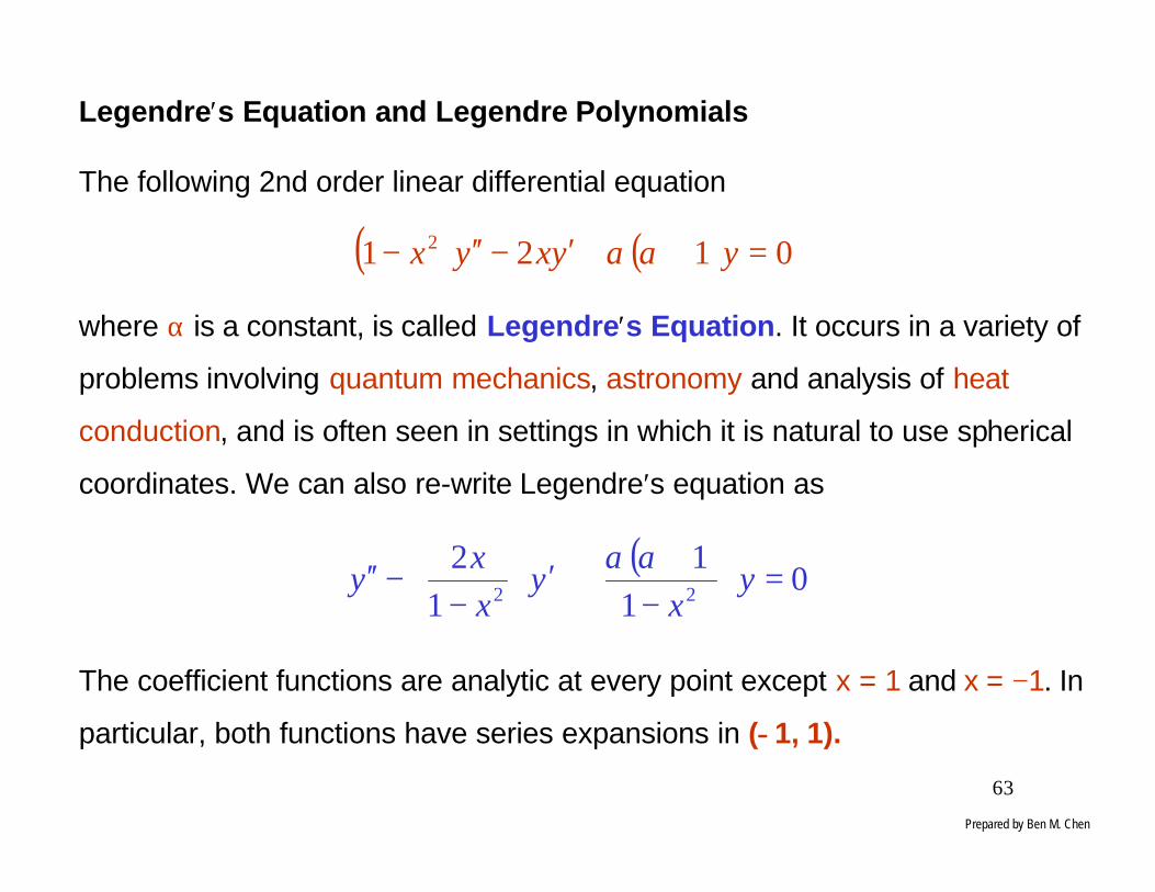
Legendre′s Equation and Legendre Polynomials

The following 2nd order linear differential equation

( ) ( ) 0121 2 =++′−′′− yyxyx αα

where α is a constant, is called Legendre′s Equation. It occurs in a variety of

problems involving quantum mechanics, astronomy and analysis of heat

conduction, and is often seen in settings in which it is natural to use spherical

coordinates. We can also re-write Legendre′s equation as

( )0

1

1

1

222

=

−+

+′

−−′′ y

xy

xx

yαα

The coefficient functions are analytic at every point except x = 1 and x = −1. In

particular, both functions have series expansions in (−−1, 1).


64

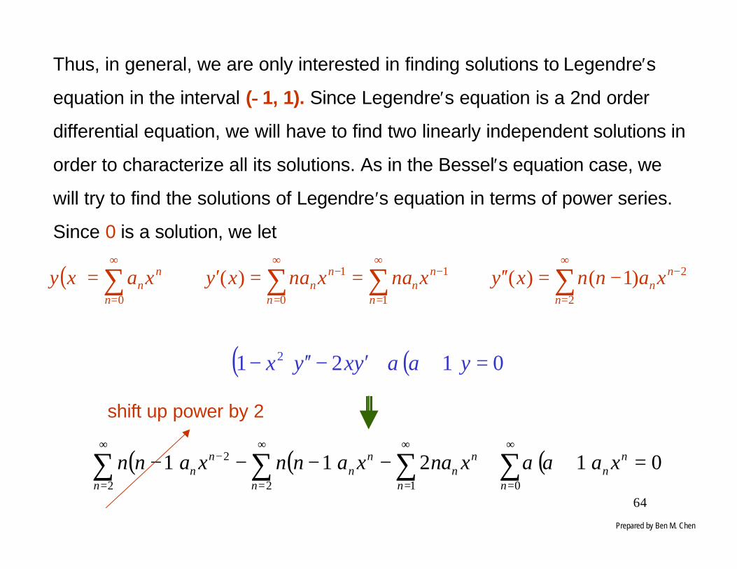
Thus, in general, we are only interested in finding solutions to Legendre′s

equation in the interval (−−1, 1). Since Legendre′s equation is a 2nd order

differential equation, we will have to find two linearly independent solutions in

order to characterize all its solutions. As in the Bessel′s equation case, we

will try to find the solutions of Legendre′s equation in terms of power series.

Since 0 is a solution, we let

( ) ∑∑∑∑∞

=

−∞

=

−∞

=

−∞

=

−=′′⇒==′⇒=2

2

1

1

0

1

0

)1()()(n

nn

n

nn

n

nn

n

nn xannxyxnaxnaxyxaxy

( ) ( ) 0121 2 =++′−′′−

+

yyxyx αα

( ) ( ) ( ) 012110122

2 =++−−−− ∑∑∑∑∞

=

∞

=

∞

=

∞

=

−

n

nn

n

nn

n

nn

n

nn xaxnaxannxann αα

shift up power by 2


65

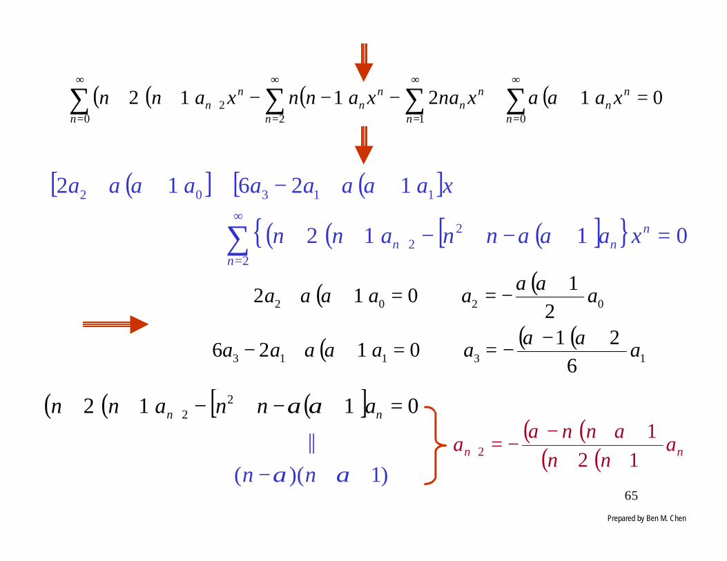
( )( ) ( ) ( ) 0121120120

2 =++−−−++ ∑∑∑∑∞

=

∞

=

∞

=

∞

=+

n

nn

n

nn

n

nn

n

nn xaxnaxannxann αα

( )[ ] ( )[ ]

( )( ) ( )[ ]{ }∑∞

=+ =+−+−+++

++−+++

2

22

11302

0112

12612

n

nnn xannann

xaaaaa

αα

αααα

( ) ( )

( ) ( )( )13113

0202

621

0126

21

012

aaaaa

aaaa

+−−=⇒=++−

+−=⇒=++

αααα

αααα

( )( ) ( )[ ] 0112 22 =+−+−++ + nn annann αα

)1)((

||

++− αα nn

( )( )( )( ) nn a

nnnn

a12

12 ++

++−−=+

αα


66

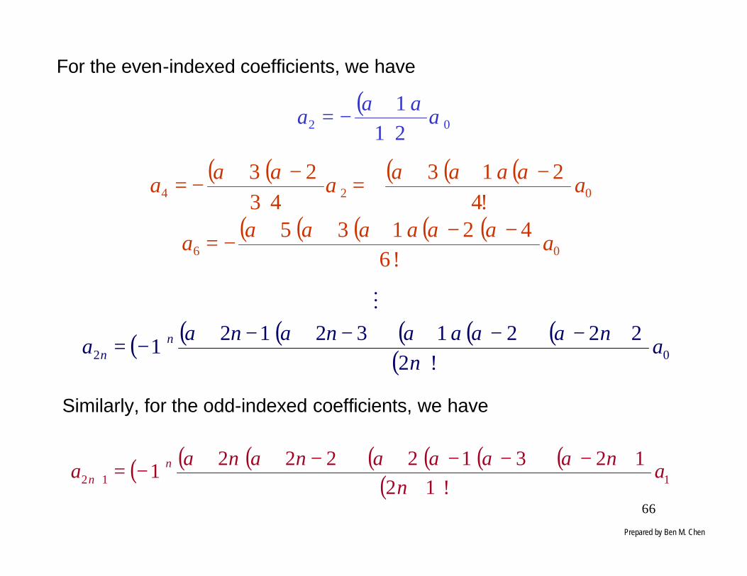
For the even-indexed coefficients, we have

( )02 21

1α

αα⋅

+−=a

( )( ) ( )( ) ( )

( )( )( ) ( )( )06

024

!642135

!4

213

43

23

aa

aa

−−+++−=

−+++=⋅

−+−=

αααααα

ααααααα

( ) ( )( ) ( ) ( ) ( )( ) 02 !2

222132121 a

nnnn

a nn

+−⋅⋅⋅−+⋅⋅⋅−+−+−=

ααααααM

Similarly, for the odd-indexed coefficients, we have

( ) ( )( ) ( )( )( ) ( )( ) 112 !12

123122221 a

nnnn

a nn +

+−⋅⋅⋅−−+⋅⋅⋅−++−=+αααααα


67

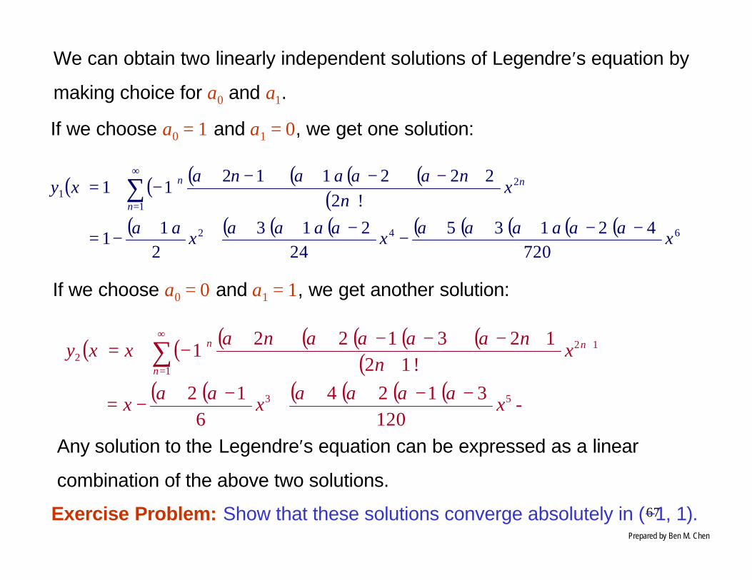
We can obtain two linearly independent solutions of Legendre′s equation by

making choice for a0 and a1.

If we choose a0 = 0 and a1 = 1, we get another solution:

( ) ( ) ( ) ( )( )( ) ( )( )

( )( ) ( )( )( )( )⋅⋅⋅−−+++−+−=

++−⋅⋅⋅−−+⋅⋅⋅+

−+= ∑∞

=

+

-120

31246

12

!12123122

1

53

1

122

xxx

xn

nnxxy

n

nn

αααααα

ααααα

Exercise Problem: Show that these solutions converge absolutely in (−1, 1).

( ) ( ) ( ) ( ) ( ) ( )( )

( ) ( )( ) ( ) ( )( )( ) ( )( )⋅⋅⋅+−−+++−−++++−=

+−⋅⋅⋅−+⋅⋅⋅−+−+= ∑

∞

=

642

1

21

72042135

24213

21

1

!2

22211211

xxx

xn

nnxy

n

nn

αααααααααααα

ααααα

If we choose a0 = 1 and a1 = 0, we get one solution:

Any solution to the Legendre′s equation can be expressed as a linear

combination of the above two solutions.


68

Recall that the first solution,

( ) ( )( ) ( ) ( )( )( ) ( )( ) ⋅⋅⋅+−−+++−−++++−= 6421 720

4213524

21321

1)( xxxxyαααααααααααα

When α = 0, we have1)(1 =xy

When α = 2, we have ( ) 221 31

2212

1)( xxxy −=+−=

When α = 4, we have

( ) 42421 3

35101

24)24(4)14)(34(

2414

1)( xxxxxy +−=−++++−=

Note that all the above solutions are polynomials, this process can be carried

on for any even integer α.


69

Similarly, one can obtain polynomial solutions for odd integer α from

( )( ) ( )( )( )( )⋅⋅⋅−−+++−+−= -

120

3124

6

12)( 53

2 xxxxyαααααα

1)(2 == αxxy

( )( )

M

33

5

6

1323)( 33

2 =−=−+

−= αxxxxxy

In fact, whenever α is a nonnegative integer, the power series for either y1(x)

(if α is even) or y2(x) (if α is odd) reduces to a finite series, and we obtain a

polynomial solution of Legendre′s equation. Such polynomial solutions are

useful in many applications, including methods for approximating solutions of

equations f (x) = 0.Prepared by Ben M. Chen

70

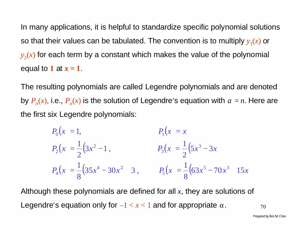
In many applications, it is helpful to standardize specific polynomial solutions

so that their values can be tabulated. The convention is to multiply y1(x) or

y2(x) for each term by a constant which makes the value of the polynomial

equal to 1 at x = 1.

The resulting polynomials are called Legendre polynomials and are denoted

by Pn(x), i.e., Pn(x) is the solution of Legendre′s equation with α = n. Here are

the first six Legendre polynomials:

( ) ( )

( ) ( ) ( ) ( )

( ) ( ) ( ) ( )xxxxPxxxP

xxxPxxP

xxPxP

1570638

1 ,33035

8

1

352

1 ,13

2

1

,1

355

244

33

22

10

+−=+−=

−=−=

==

Although these polynomials are defined for all x, they are solutions of

Legendre′s equation only for –1 < x < 1 and for appropriate α.Prepared by Ben M. Chen

71

-1 -0.8 -0.6 -0.4 -0.2 0 0.2 0.4 0.6 0.8 1-1.5

-1

-0.5

0

0.5

1

1.5

Legendre Polynomials

P0

P1

P2

P3 P4

P5

1

Legendre Polynomials


72

Properties of Legendre Polynomials

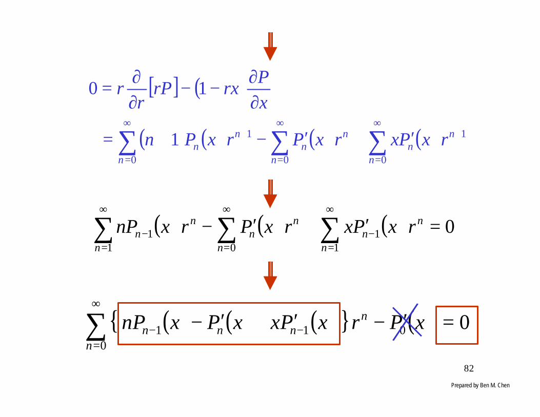
Theorem 0. If m and n are distinct nonnegative integers, ( ) ( ) 01

1

=∫−

dxxPxP nm

Proof: Note that Pn and Pm are solutions of Legendre′s differential equations

with α = n and α = m, respectively. Hence, we have

( ) ( )( ) ( ) mmm

nnn

PmmPxPx

PnnPxPx

1210

12102

2

++′−′′−=

++′−′′−=

( ) ( )( ) ( ) nmnmnm

mnmnmn

PPmmPPxPPx

PPnnPPxPPx

1210

12102

2

++′−′′−=

++′−′′−=

n

m

P

P

××

subtract these two equations –

( )( ) ( ) ( ) ( )[ ] 01121 2 =+−++′−′−′′−′′−= nmnmmnnmmn PPmmnnPPPPxPPPPx

nmmnmnmn PPPPPPPP ′′−′′−′′+′′=

( ) [ ] [ ] ( ) ( )[ ] nmnmmnnmmn PPnnmmPPPPxPPPPdxd

x 1121 2 +−+=′−′−′−′−


73

( ) [ ] [ ] ( ) ( )[ ] nmnmmnnmmn PPnnmmPPPPxPPPPdxd

x 1121 2 +−+=′−′−′−′−

( )( )[ ] ( ) ( )[ ] nmmmn PPnnmmPPPPxdxd

111 2 +−+=′−′−

( )( )[ ] ( ) ( )[ ] dxxPxPnnmmdxPPPPxdx

dnmmmn )()(111

1

1

1

1

2 ∫∫−−

+−+=′−′−

( ) ( )[ ] 0)()(111

1

=+−+ ∫−

dxxPxPnnmm nm

( )( )[ ] ( )( ) 0111

1

21

1

2 =′−′−=′−′−−

−∫ PPPPxdxPPPPx

dx

dmmnmmn

nmdxxPxP nm ≠=∫−

since,0)()(1

1


74

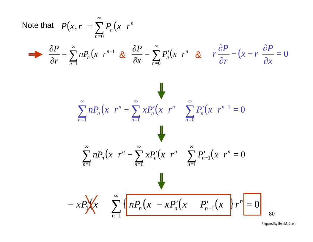
Generating Function for Legendre Polynomials

The generating function for Legendre Polynomials is

( ) ( ) 21

221,−

+−= rxrrxP

To see why this is called a generating function, recall the binomial expansion

( ) ⋅⋅⋅++++=− − 3221

2

5

2

3

2

1

!3

1

2

3

2

1

!2

1

2

111 zzzz

Let , we have22 rxrz −=

( ) ( ) ( ) ( ) ⋅⋅⋅+−+−+−+=32222 2

16

52

8

32

2

11, rxrrxrrxrrxP

Re-write it as a power series of r,

( ) ⋅⋅⋅+

+−+

+−++= 3322

2

5

2

3

2

3

2

11, rxxrxxrrxP

P0 P2 P3P1

……

∑∞

=

=0

)(n

nn rxP


75

Theorem 1. (Recurrence Relation of Legendre Polynomial) For each positive

integer n and for all ,11 ≤≤− x

( ) ( ) ( ) ( ) ( ) 0121 11 =++−+ −+ xnPxxPnxPn nnn

Proof: Differentiating the generating function

( ) ( ) 21221,−

+−= rxrrxP

w.r.t. r, we obtain

( ) ( ) ( ) )(2122212

1 232232 rxrxrrxrxrrP

−+−=+−+−−=∂∂ −−

( ) ( ) ( ) ),()(21212122 rxPrxrxrxr

rP

rxr −=−+−=∂∂+− −


76

Noting that from the property of the generating function, i.e.,

( ) ( )∑∞

=

=0

,n

nn rxPrxP

we have

( ) ( )∑∑∞

=

−∞

=

− ==∂∂

1

1

0

1

n

nn

n

nn rxnPrxnP

rP

Substitute this into the equation we derived, i.e.,

( ) ),()(21 2 rxPrxrP

rxr −=∂∂+−

( ) ( ) ( ) ( ) ( )∑ ∑∑∑∑∞

=

∞

=

+∞

=

+∞

=

∞

=

− =+−+−0 0

1

1

1

11

1 02n n

nn

nn

n

nn

n

nn

n

nn rxPrxxPrxnPrxxnPrxnP

( ) ( ) ( ) ( ) ( )∑ ∑∑∑∑∞

=

∞

=−

∞

=−

∞

=

∞

=+ =+−−+−++

0 11

21

101 0)1()2()1(

n n

nn

nn

n

nn

n

nn

n

nn rxPrxxPrxPnrxPxnrxPn

( ) ( )∑∑∞

=

∞

=

− =−−+−01

12 0)()21(n

nn

n

nn rxPrxrxnPrxr


77

( ) ( )[ ] ( ) ( ) ( ) ( ) ( )[ ]

( ) ( ) ( ) ( ) ( ){ } 0121

1211

211

01201

=++−++

++−++−

∑∞

=−+

n

nnnn rxnPxxPnxPn

rxPxxPxPxxPxP

( ) ( )( ) ( ) ( ) ( ) ( ) 01211

0

012

01

=++−+=−

xPxxPxP

xxPxP

and, for n = 2, 3, 4, ⋅ ⋅ ⋅

( ) ( ) ( ) ( ) ( ) 0121 11 =++−+ −+ xnPxxPnxPn nnn

( ) ( ) ( ) ( ) ( ) ( )

( ) ( ) ( ) ( ) ( ) ( ) ( ){ } n

nnnnnn rxPxxPxPnxxnPxPn

rxPrxxPxxPrxxPrxPxP

∑∞

=−−+ +−−+−++

+−−−+=

2111

010121

121

220


78

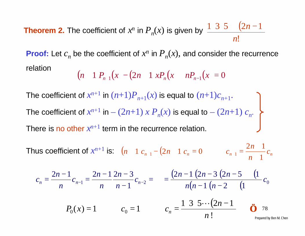
Theorem 2. The coefficient of xn in Pn(x) is given by ( )!

12531

nn −⋅⋅⋅⋅⋅

Proof: Let cn be the coefficient of xn in Pn(x), and consider the recurrence

relation( ) ( ) ( ) ( ) ( ) 0121 11 =++−+ −+ xnPxxPnxPn nnn

The coefficient of xn+1 in (n+1)Pn+1(x) is equal to (n+1)cn+1.

The coefficient of xn+1 in – (2n+1) x Pn(x) is equal to – (2n+1) cn.

There is no other xn+1 term in the recurrence relation.

Thus coefficient of xn+1 is: ( ) ( ) nnnn cnn

ccncn1

120121 11 +

+=⇒=+−+ ++

( )( )( ) ( )( )( ) ( ) 021 121

1523212

1

321212c

nnnnnn

cnn

nn

cn

nc nnn ⋅⋅⋅−−

⋅⋅⋅−−−=⋅⋅⋅=

−−−

=−

= −−

( )!

1253111)( 00 n

nccxP n

−⋅⋅=⇒=⇒=

L √√Prepared by Ben M. Chen

79

Theorem 3. For each positive integer n,

( ) ( ) ( ) 01 =′+′− − xPxPxxnP nnn

Proof. Differentiating the generating function w.r.t. x,

we obtain

( ) ( ) 21

221,−

+−= rxrrxP

( )( ) ( ) ( ) ),(21212122

1

2122232 rxrPrxrrxP

rxrrxrrxP

=+−=∂∂

+−⇒+−−−=∂∂ −−

We′ve proved in Theorem 1 that

( ) ),()(21 2 rxPrxrP

rxr −=∂∂+−

( )xP

rxrPrxr

∂∂=+− ),(21 2

( )rP

rxPrxrxr

∂∂

−=+− ),()(21 2

rP

rxPrx

xP

rxrP

∂∂

−=

∂∂

),()(),(

( ) 0=∂∂−−

∂∂

xP

rxrP

r


80

( ) ( ) ( ) 00

1

01

=′+′− ∑∑∑∞

=

+∞

=

∞

= n

nn

n

nn

n

nn rxPrxPxrxnP

( ) ( ) ( ) ( ){ } 01

10 =′+′−+′− ∑∞

=−

n

nnnn rxPxPxxnPxPx

( ) ( ) ( ) 0 1

101

=′+′− ∑∑∑∞

=−

∞

=

∞

= n

nn

n

nn

n

nn rxPrxPxrxnP

Note that ( ) ( ) n

nn rxPrxP ∑

∞

=

=0

,

( ) 1

1

−∞

=∑=

∂∂ n

nn rxnP

rP ( ) n

nn rxP

xP ∑

∞

=

′=∂∂

0& ( ) 0=

∂∂−−

∂∂

xP

rxrP

r&


81

Theorem 4. For each positive integer n,

( ) ( ) ( ) 011 =′+′− −− xPxxPxnP nnn

Proof: We had in the previous proof the following equalities

( ) ( ) ( )xP

rxrP

rxP

rxrrxrP∂∂−=

∂∂

∂∂+−= &21, 2

( )[ ]rP

rrxrPrxrPr

r∂∂+=

∂∂ 2),(,

Next,

( )[ ] ( ) ( )

( )xP

rx

xP

rxrxP

rxrrxrPr

r

∂∂

−=

∂∂

−+∂∂

+−=∂∂

1

21, 2

( )[ ] ( ) 01, =∂∂−−

∂∂

xP

rxrxrPr

r

( ) ( )

( )∑

∑∞

=

∞

=

′=∂∂⇒

=

0

0

,

n

nn

n

nn

rxPxP

rxPrxP

( )[ ] ( )

( )∑

∑∞

=

+

∞

=

+

+=

∂∂

=∂∂

0

1

0

1

)1(

,

n

nn

n

nn

rxPn

rxPr

rrxrPr

r


82

( ) ( ) ( ) 01

101

1 =′+′− ∑∑∑∞

=−

∞

=

∞

=−

n

nn

n

nn

n

nn rxPxrxPrxnP

( ) ( ) ( ){ } ( ) 00

011 =′−′+′−∑∞

=−−

n

nnnn xPrxPxxPxnP

[ ] ( )

( ) ( ) ( ) ( )∑∑∑∞

=

+∞

=

∞

=

+ ′+′−+=

∂∂−−

∂∂=

0

1

00

11

10

n

nn

n

nn

n

nn rxPxrxPrxPn

xP

rxrPr

r


83

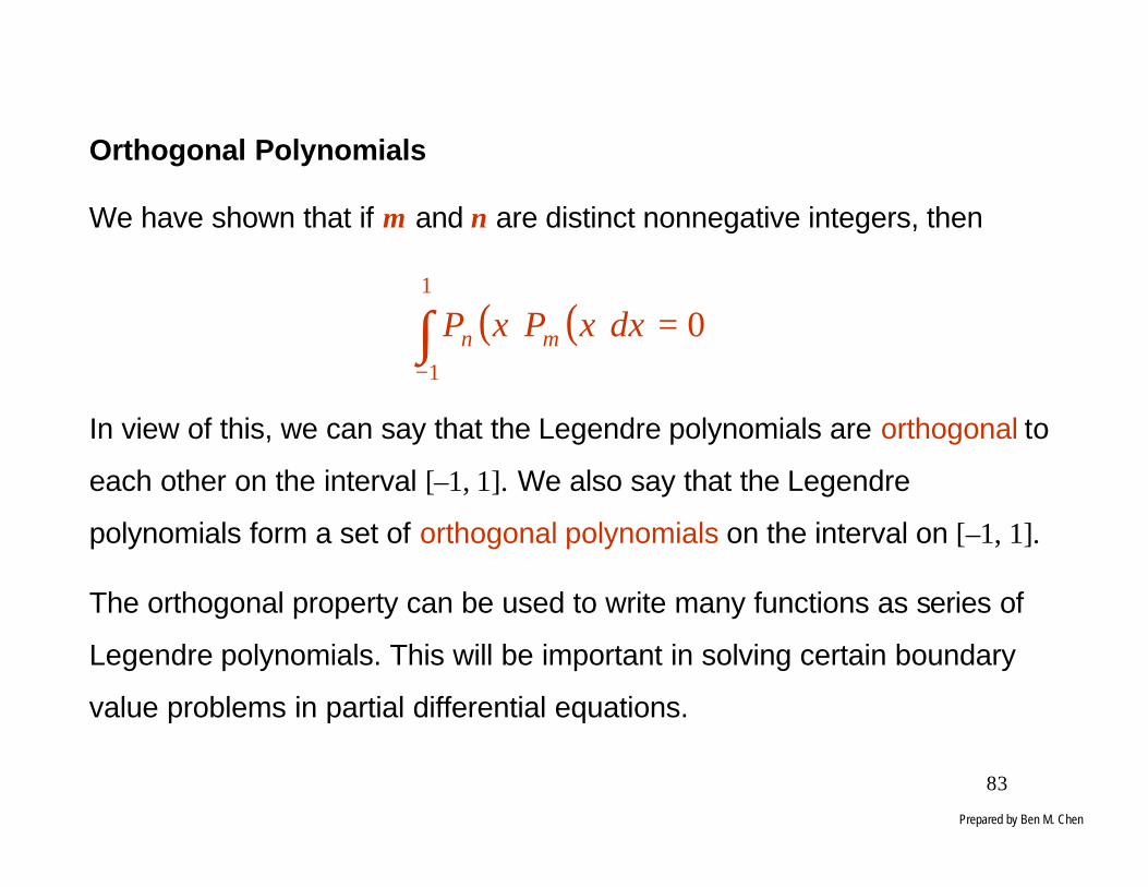
Orthogonal Polynomials

We have shown that if m and n are distinct nonnegative integers, then

In view of this, we can say that the Legendre polynomials are orthogonal to

each other on the interval [–1, 1]. We also say that the Legendre

polynomials form a set of orthogonal polynomials on the interval on [–1, 1].

The orthogonal property can be used to write many functions as series of

Legendre polynomials. This will be important in solving certain boundary

value problems in partial differential equations.

( ) ( ) 01

1

=∫−

dxxPxP mn


84

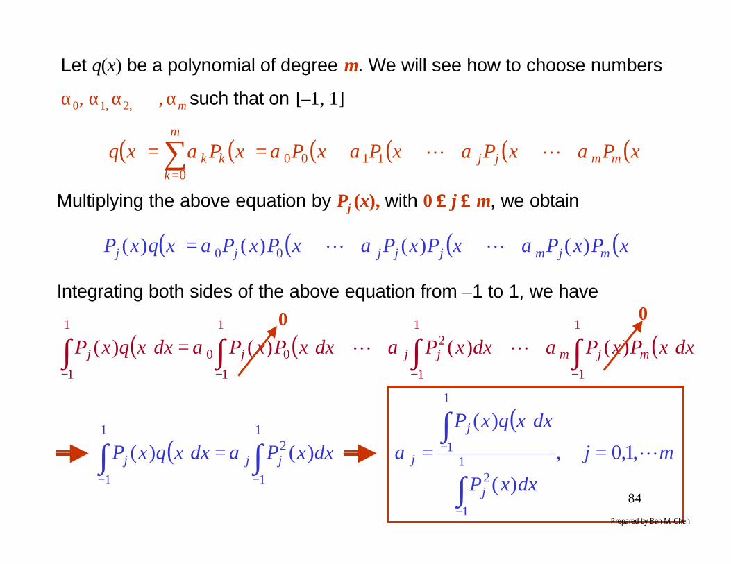
Let q(x) be a polynomial of degree m. We will see how to choose numbers

α0, α1, α2, ⋅ ⋅ ⋅, αm such that on [–1, 1]

( ) ( ) ( ) ( ) ( ) ( )xPxPxPxPxPxq mmjj

m

kkk ααααα +++++== ∑

=

LL11000

Multiplying the above equation by Pj (x), with 0 ≤≤ j ≤≤ m, we obtain

( ) ( ) ( ) ( )xPxPxPxPxPxPxqxP mjmjjjjj )()()()( 00 ααα ++++= LL

Integrating both sides of the above equation from –1 to 1, we have

( ) ( ) ( )∫∫∫∫−−−−

++++=1

1

1

1

21

1

00

1

1

)()()()( dxxPxPdxxPdxxPxPdxxqxP mjmjjjj ααα LL

00

( ) ∫∫−−

=1

1

21

1

)()( dxxPdxxqxP jjj α

( )mj

dxxP

dxxqxP

j

j

j L,1,0,

)(

)(

1

1

2

1

1 ==

∫

∫

−

−α


85

( ) ( ) ( )

( ) ( ) ( ) xxxxPxPx

xxPxPx

53

3521

52

53

52

31

1321

32

31

32

313

3

202

2

+

−=+=

+

−=+=

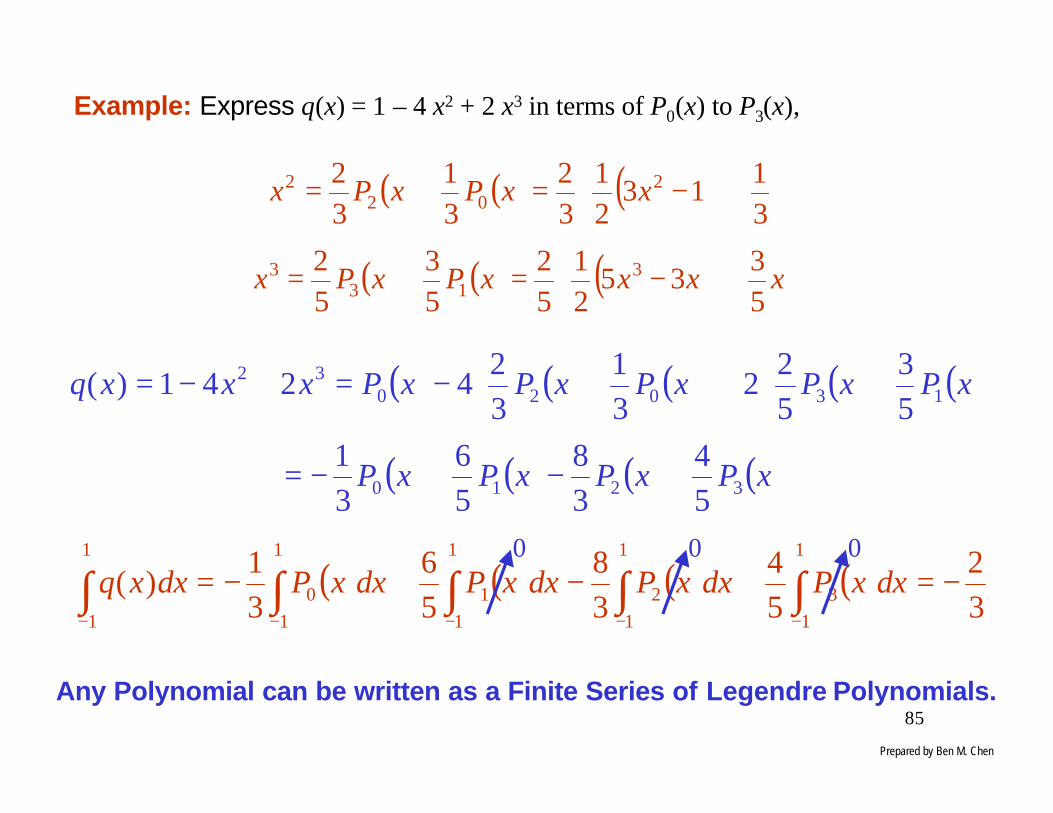
Example: Express q(x) = 1 – 4 x2 + 2 x3 in terms of P0(x) to P3(x),

Any Polynomial can be written as a Finite Series of Legendre Polynomials.

( ) ( ) ( ) ( ) ( )

( ) ( ) ( ) ( )xPxPxPxP

xPxPxPxPxPxxxq

3210

1302032

5

4

3

8

5

6

3

1

5

3

5

22

3

1

3

24241)(

+−+−=

++

+−=+−=

( ) ( ) ( ) ( )3

2

5

4

3

8

5

6

3

1)(

1

1

3

1

1

2

1

1

1

1

1

0

1

1

−=+−+−= ∫∫∫∫∫−−−−−

dxxPdxxPdxxPdxxPdxxq0 0 0


86

Theorem 5. Let m and n be nonnegative integers, with m < n. Let q(x) be any

polynomial of degree m. Then

( ) ( ) 01

1

=∫−

dxxPxq n

That is, the integral, from –1 to 1, of a Legendre polynomial multiplied by

any polynomial of lower degree, is zero.

Proof: We have shown that for any polynomial q(x) of degree m, there exist

scalar α0, α1, ⋅ ⋅ ⋅ αm such that

( ) ( ) ( ) ( )xPxPxPxq mmααα +⋅⋅⋅++= 1100

( ) ( ) ( ) ( ) ( ) ( ) ( ) ( )∫∫∫∫−−−−

+⋅⋅⋅++=1

1

1

1

11

1

1

00

1

1

dxxPxPdxxPxPdxxPxPdxxPxq nmmnnn ααα0 0 0

= 0Prepared by Ben M. Chen

87

Theorem 6. For any nonnegative integer n,

( )[ ]12

21

1

2

+=∫

− ndxxPn

Proof: Let cn be coefficient of x n in Pn(x) and also let the coefficient of xn–1

in Pn–1(x) be cn–1. Define

( ) ( ) ( ) ( )?????

??

2111

211

1

11

1

+++=−−−++=

++−++=−=

−−−−

−−−

−

−−

−

LLL

LL

nnnnn

nnn

nnn

n

nnnnn

n

nn

xxxxcxxc

xxcxcc

xxcxxPcc

xPxq

Thus, q(x) has degree n – 1 or lower.

( ) ( ) ( )xqxxPcc

xP nn

nn += −

−1

1

( )[ ] ( ) ( ) ( ) ( ) ( ) ( ) ( )xPxqxPxxPcc

xqxxPcc

xPxP nnnn

nn

n

nnn +=

+= −

−−

−1

11

1

2


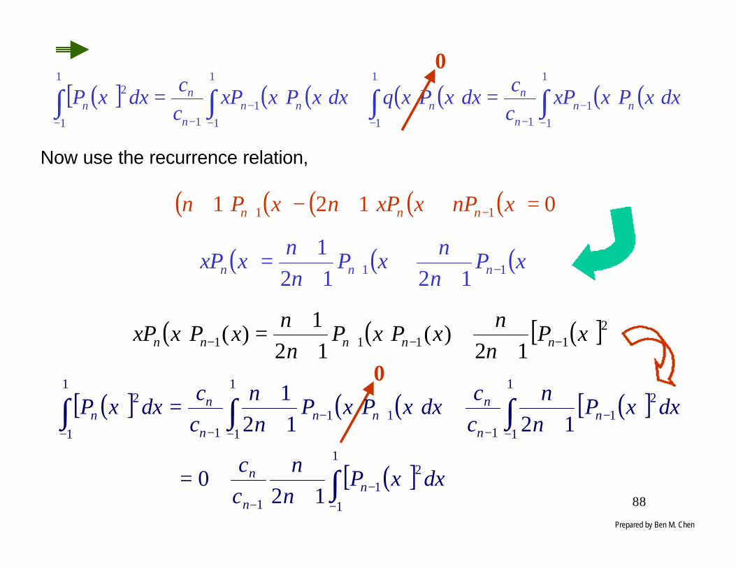
88

( )[ ] ( ) ( ) ( ) ( ) ( ) ( )∫∫∫∫−

−−−−

−−−

=+=1

1

11

1

1

1

1

11

1

1

2 dxxPxxPcc

dxxPxqdxxPxxPcc

dxxP nnn

nnnn

n

nn

0

Now use the recurrence relation,

( ) ( ) ( ) ( ) ( ) 0121 11 =++−+ −+ xnPxxPnxPn nnn

( ) ( ) ( )[ ]21111 12

)(12

1)( xP

nn

xPxPn

nxPxxP nnnnn −−+− +

++

+=

0

( ) ( ) ( )xPnn

xPnn

xxP nnn 11 1212

1−+ +

+++=

( )[ ] ( ) ( ) ( )[ ]

( )[ ]∫

∫∫∫

−−

−

−−

−−+−

−−

++=

++

++=

1

1

21

1

1

1

21

1

1

1

111

1

1

2

120

1212

1

dxxPnn

cc

dxxPnn

cc

dxxPxPnn

cc

dxxP

nn

n

nn

nnn

n

nn


89

Recall from Theorem 2 that( )!

1231

nn

cn−⋅⋅⋅⋅

=

( )( ) n

ncc

nn

cn

nn

12

!1

3231

11

−=⇒−

−⋅⋅⋅⋅=⇒−

−

( )[ ] ( )[ ] ( )[ ]∫∫∫−

−−

−− +

−=+

−=1

1

21

1

1

21

1

1

2

1212

1212

dxxPnn

dxxPnn

nn

dxxP nnn

( )[ ] ( )[ ] ( )( )( )( ) ( )[ ]

( )( )( )( )( )( ) ( )[ ]

( )[ ]12

2

12

1

35321212

13523212

1212

3212

12

12

1

1

20

1

1

20

1

1

22

1

1

21

1

1

2

+=

+=

⋅⋅⋅⋅−−+⋅⋅⋅⋅−−−

=⋅⋅⋅=

−+−−

=+−

=

∫

∫

∫∫∫

−

−

−−

−−

−

ndxxP

n

dxxPnnnnnn

dxxPnnnn

dxxPnn

dxxP nnn


90

Finally, we can write any polynomial of degree m as a finite series of

Legendre polynomials,

( ) ( ) 11for 0

≤≤−= ∑=

xxPxqm

kkkα

( ) ( )

( )[ ]( ) ( )∫

∫

∫−

−

− +==

1

1

1

1

2

1

1

2

12dxxPxq

k

dxxP

dxxPxq

k

k

k

kα

and for k = 0, 1, 2, ⋅ ⋅ ⋅, m,

Proof. It is a combination of Theorem 6 and the formula derived earlier, i.e.,

( )

[ ]mj

dxxP

dxxqxP

j

j

j L,1,0,

)(

)(

1

1

2

1

1 ==

∫

∫

−

−α


91

Boundary Value Problems in Partial Differential Equations

A partial differential equation is an equation containing one or more partial

derivatives, e.g.,

2

2

xu

tu

∂∂=

∂∂

We seek a solution u(x, t) which depends on the independent variables x and t.

A solution of a partial differential equation is a function which satisfies the

equation. For example,

( ) ( ) textxu 42cos, −=

is a solution of the above mentioned differential equation since

( ) textu 42cos4 −−=

∂∂ ( ) tex

xu 42

2

2cos4 −−=∂∂=


92

Order of a Partial Differential Equation

A partial differential equation (p.d.e.) is said to be of order n if it contains

an n-th order partial derivative but none of higher order. For example, the

following so-called Laplace equation

02

2

2

2

2

22 =

∂∂+

∂∂+

∂∂=∇

zu

yu

xu

u

is of order 2. The p.d.e. has an order of 5,

tu

tu

xu

∂∂−

∂∂=

∂∂

5

5

2

2

Linear Case

The general linear first order p.d.e. in three variables (with u as a function of

the independent variables x and y) is

( ) ( ) ( ) ( ) 0,,,, =++∂∂+

∂∂

yxguyxfyu

yxbxu

yxaPrepared by Ben M. Chen

93

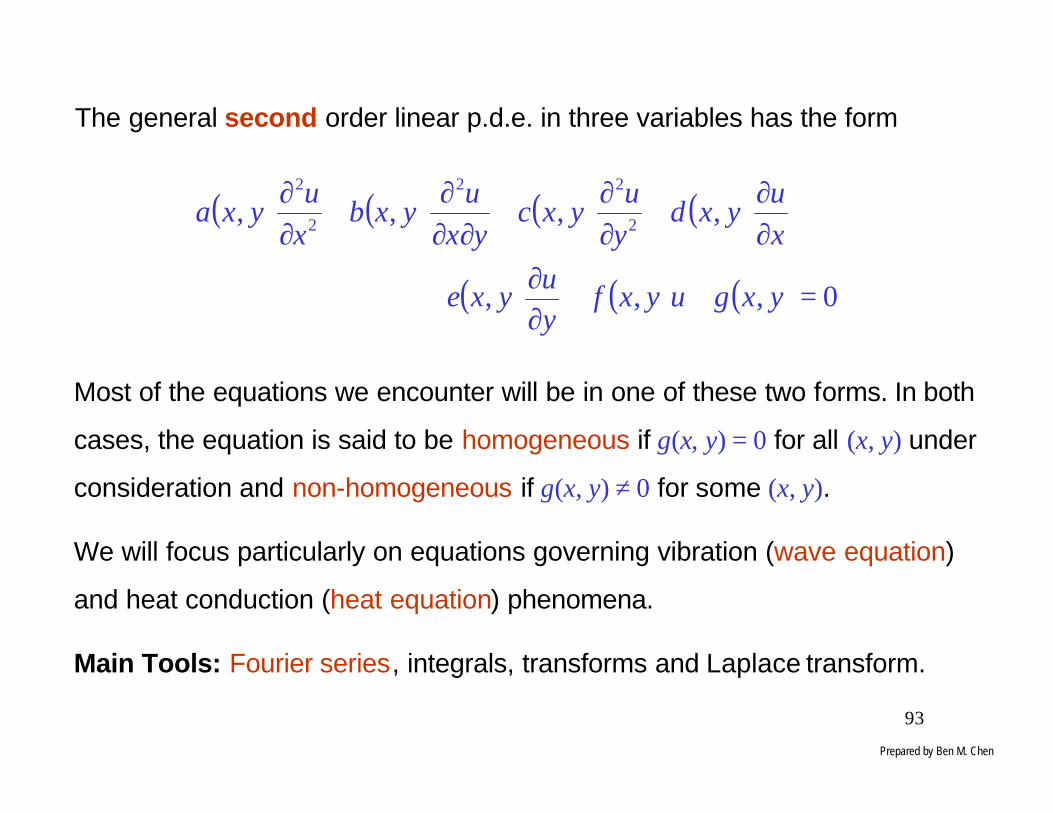
The general second order linear p.d.e. in three variables has the form

( ) ( ) ( ) ( )

( ) ( ) ( ) 0,,,

,,,, 2

22

2

2

=++∂∂+

∂∂

+∂∂

+∂∂

∂+

∂∂

yxguyxfyu

yxe

xu

yxdyu

yxcyx

uyxb

xu

yxa

Most of the equations we encounter will be in one of these two forms. In both

cases, the equation is said to be homogeneous if g(x, y) = 0 for all (x, y) under

consideration and non-homogeneous if g(x, y) ≠ 0 for some (x, y).

We will focus particularly on equations governing vibration (wave equation)

and heat conduction (heat equation) phenomena.

Main Tools: Fourier series, integrals, transforms and Laplace transform.


94

The Wave Equation

Suppose we have a flexible elastic string stretched between two pegs. We

want to describe the ensuing motion if the string is lifted and then released

to vibrate in a vertical plane.

Place the x-axis along the length of the string at the rest. At any time t and

horizontal coordinate x, let y(x, t) be the vertical displacement of the string.

0 Lx-axis

yy(x,t)

We want to determine equations which will enable us to solve for y(x, t), thus

obtaining a description of the shape of the string at any time.

x


95

We will begin by modeling a simplified case. Neglect damping forces such

as air resistance and the weight of the string and assume that the tension

T(x, t) in the string always acts tangentially to the string. Assume that the

string can only move is the vertical direction, i.e., the horizontal tension is

constant. Also assume that the mass ρρ per unit length is a constant.

Applying Newton′s 2nd Law of motion to the segment of the string between x

and x + ∆∆x, we have

Net force due to tension = Segment mass

×× Acceleration of the center of mass of the segment

For small ∆∆x, consideration of the vertical component of the equation gives

us approximately:

maF =⇔


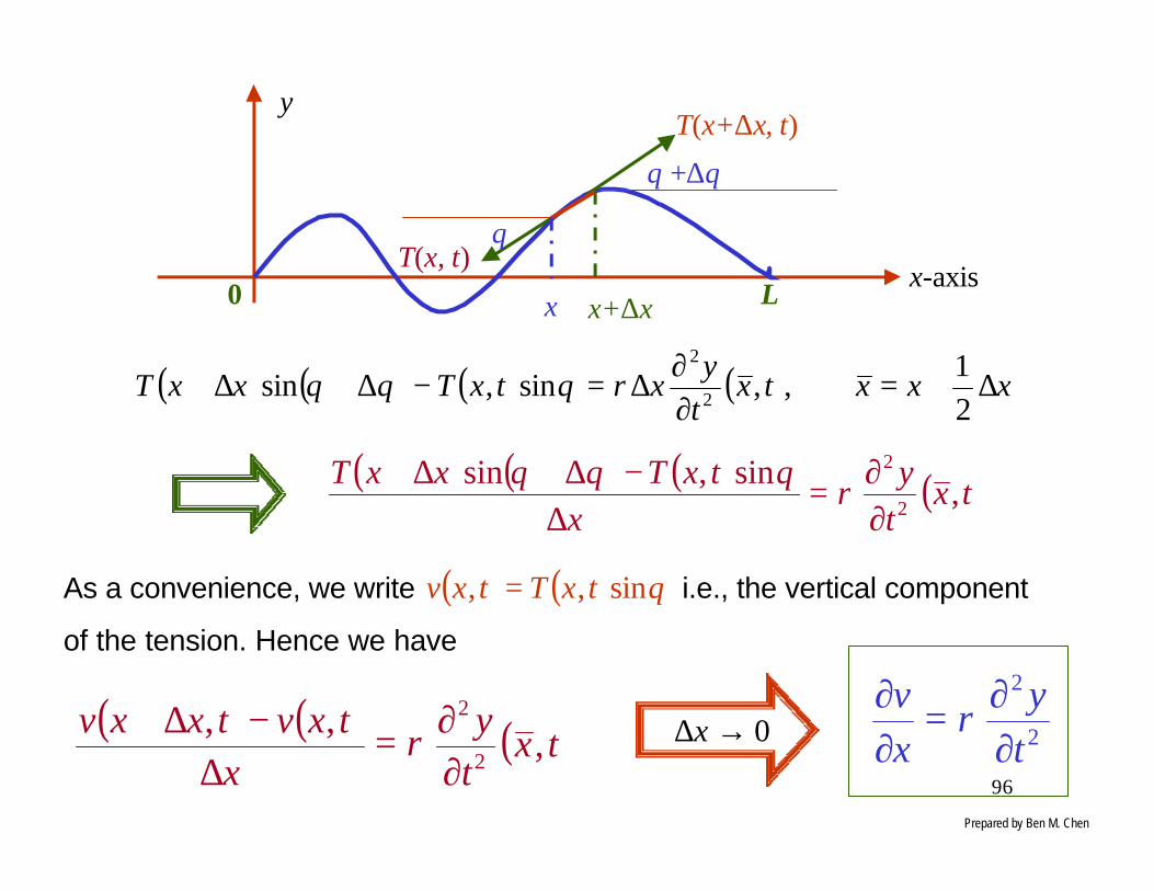
96

0 Lx-axis

yT(x+∆x, t)

x+∆x

θ +∆θ

θT(x, t)

x

( ) ( ) ( ) ( ) xxxtxty

xtxTxxT ∆+=∂∂∆=−∆+∆+

21

,,sin,sin 2

2

ρθθθ

( ) ( ) ( ) ( )txty

xtxTxxT

,sin,sin

2

2

∂∂=

∆−∆+∆+ ρθθθ

As a convenience, we write i.e., the vertical component

of the tension. Hence we have

( ) ( ) θsin,, txTtxv =

( ) ( ) ( )txty

xtxvtxxv

,,,

2

2

∂∂=

∆−∆+ ρ 2

2

ty

xv

∂∂=

∂∂ ρ0→∆x


97

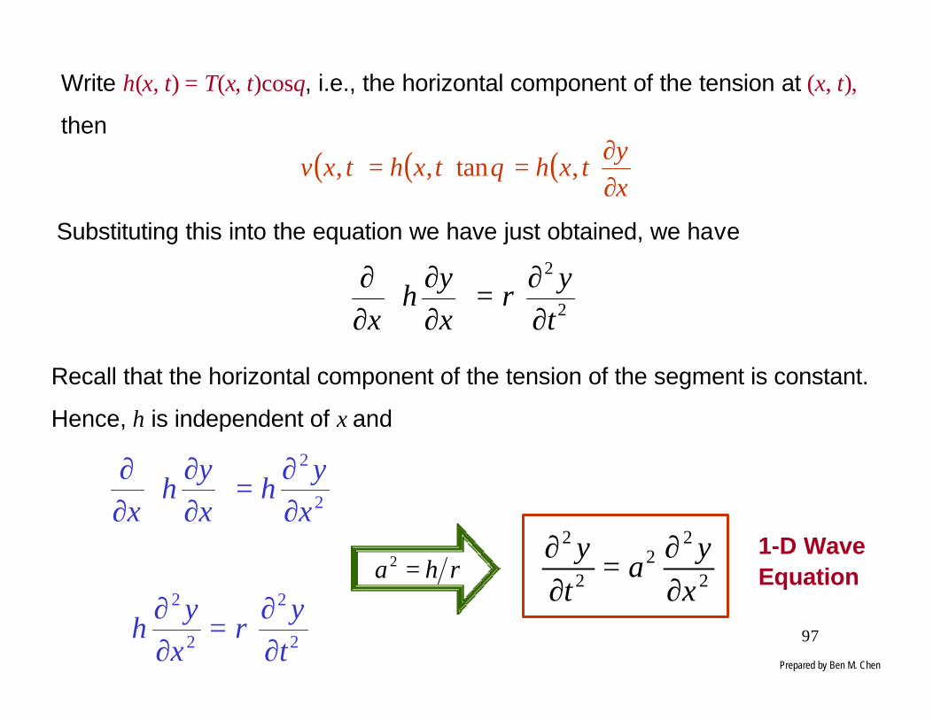
Write h(x, t) = T(x, t)cosθ, i.e., the horizontal component of the tension at (x, t),

then

( ) ( ) ( )xy

txhtxhtxv∂∂

== ,tan,, θ

Substituting this into the equation we have just obtained, we have

2

2

ty

xy

hx ∂

∂=

∂∂

∂∂

ρ

Recall that the horizontal component of the tension of the segment is constant.

Hence, h is independent of x and

2

2

2

2

2

2

ty

xy

h

xy

hxy

hx

∂∂

=∂∂

⇓

∂∂

=

∂∂

∂∂

ρ

ρha =22

22

2

2

xy

aty

∂∂=

∂∂ 1-D Wave

Equation


98

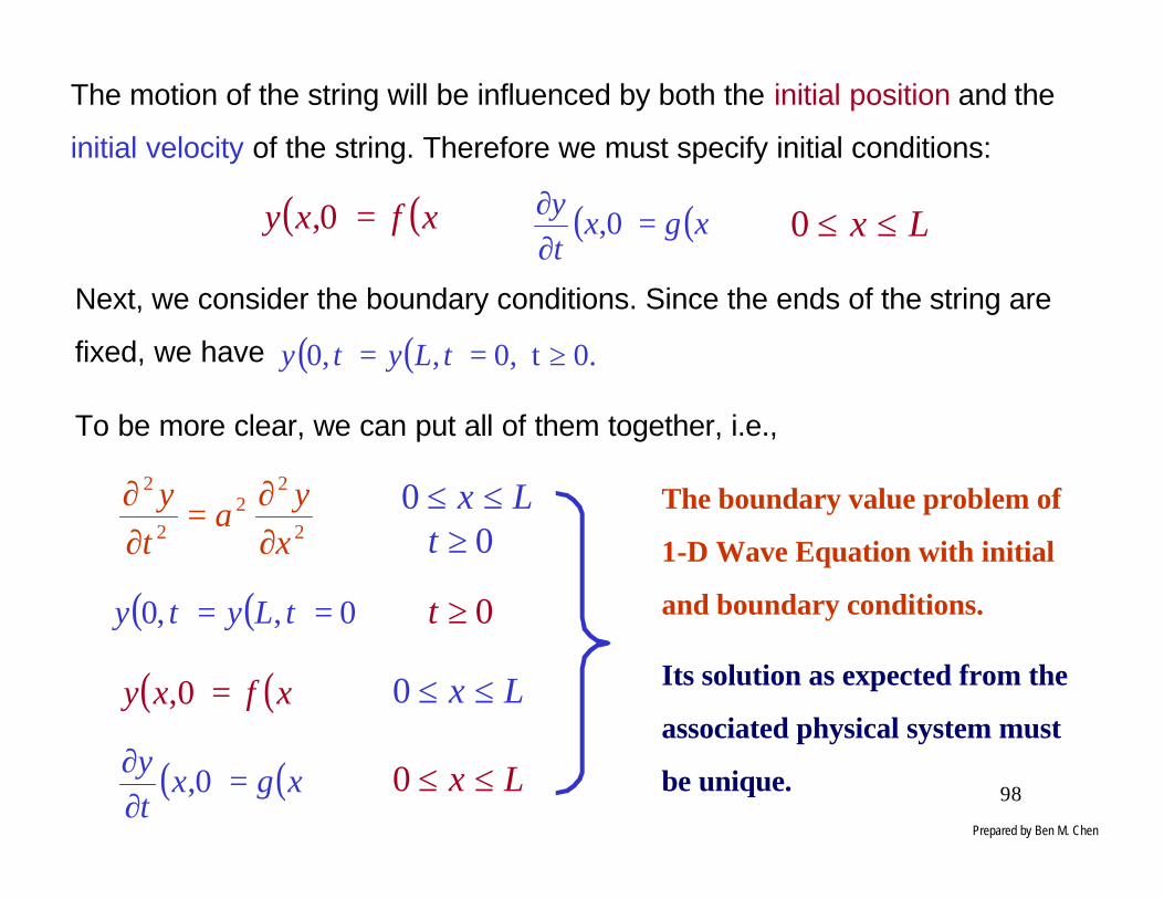
The motion of the string will be influenced by both the initial position and the

initial velocity of the string. Therefore we must specify initial conditions:

( ) ( )xfxy =0, ( ) ( )xgxty =

∂∂

0,

Next, we consider the boundary conditions. Since the ends of the string are

fixed, we have ( ) ( ) 0. t,0,,0 ≥== tLyty

Lx ≤≤0

To be more clear, we can put all of them together, i.e.,

2

22

2

2

xy

aty

∂∂=

∂∂

( ) ( ) 0,,0 == tLyty

( ) ( )xfxy =0,

( ) ( )xgxty =

∂∂

0,

Lx ≤≤0

0≥t

Lx ≤≤0

Lx ≤≤0

0≥tThe boundary value problem of

1-D Wave Equation with initial

and boundary conditions.

Its solution as expected from the

associated physical system must

be unique.


99

The Heat Equation

This is to study temperature distribution in a straight, thin bar under simple

circumstances. Suppose we have a straight, thin bar of constant density ρ

and constant cross-sectional area A placed along the x-axis from 0 to L.

Assume that the sides of the bar are insulated and so not allow heat loss

and that the temperature on the cross-section of the bar perpendicular to the

x-axis at x is a function u(x, t) of x and t, independent of y.

Let the specific heat of the bar be c, and let the thermal conductivity be k,

both constant. Now consider a typical segment of the bar between x = α and

x = β.

0L

x

y

α β

u(x, t)


100

By the definition of specific heat, the rate at which heat energy accumulates

in this segment of the bar is:

∫ ∂∂β

α

ρ dxtu

Ac

By Newton′s law of cooling, heat energy flows within this segment from the

warmer to the cooler end at a rate equal to k times the negative of the

temperature gradient. Therefore, the net rate at which heat energy enters

the segment of bar between α and β at time t is:

( ) ( )txu

kAtxu

kA ,, αβ∂∂−

∂∂

In the absence of heat production within the segment, the rate at which heat

energy accumulates within the segment must balance the rate at which heat

energy enters the segment. Hence,

( ) ( )txu

kAtxu

kAdxtu

Ac ,, αβρβ

α ∂∂−

∂∂=

∂∂

∫Prepared by Ben M. Chen

101

( ) ( ) ∫ ∂∂=

∂∂−

∂∂ β

α

αβ dxxu

kAtxu

kAtxu

kA2

2

,,

Note that

02

2

=

∂∂−

∂∂

∫β

α

ρ dxxu

kAtu

Ac 02

2

=∂∂

−∂∂

xu

kAtu

Acρ

This is the so-called heat equation, which is more customary written as:

2

22

xu

atu

∂∂=

∂∂

where a2 = k/(cρ) is called the thermal diffusive of the bar. To determine u

uniquely, we need boundary conditions (information at the ends of the bar)

and initial conditions (temperature throughout the bar at time zero). The

p.d.e. together with these pieces of information, constitutes a boundary

value problem for the temperature function u.


102

( ) ( )( ) ( ) )0( 0,

)0( ,,0

)00( 2

22

L x xfxu

t TtLutu

L, t x xu

atu

<<=>==

><<∂∂=

∂∂

Problem 1. Both ends of the bar are kept in a constant temperature.

( ) ( )

( ) ( ) )0( 0,

)0( 0,,0

)00( 2

22

L x xfxu

t tLtu

ttu

L, t x xu

atu

<<=

>=∂∂=

∂∂

><<∂∂=

∂∂

Problem 2. No heat flows across the ends of the bar.

Reading assignment: Laplace′s Equation; Poisson′s Equation; Dirichlet and

Neumann Problems; Laplace′s Equation in Cylindrical & Spherical Coordinates


103

Fourier Series Solution of Wave Equation

Recall the wave equation of an initially displaced vibrating string with zero initial

velocity,

This boundary value problem models the vibration of an elastic string of length

L, fastened at the ends, picked up at time zero to assume the shape of the

graph of y(x,0) = f (x) and released from rest.

Wave equation

Boundary conditions

Initial displacement

Initial velocity

2

22

2

2

xy

aty

∂∂=

∂∂

( ) ( ) 0,,0 == tLyty

( ) ( )xfxy =0,

( ) 00, =∂∂

xty

Lx ≤≤0

0≥t

Lx ≤≤0

Lx ≤≤0

0≥t


104

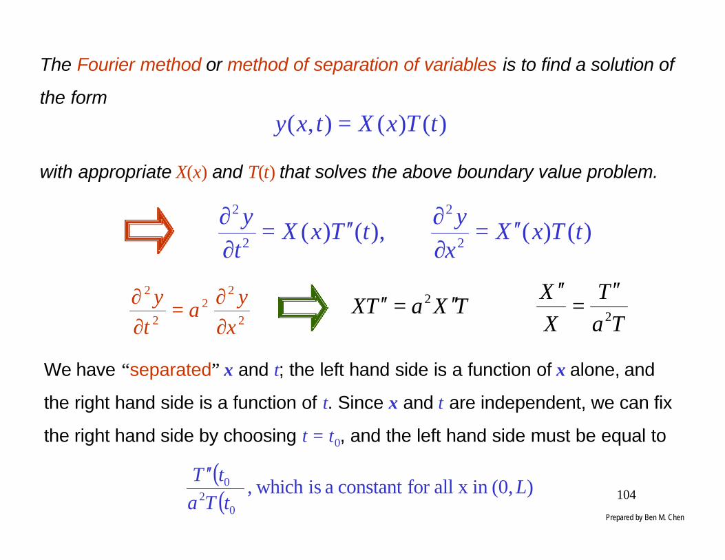
The Fourier method or method of separation of variables is to find a solution of

the form

)()(),( tTxXtxy =

with appropriate X(x) and T(t) that solves the above boundary value problem.

)()(),()(2

2

2

2

tTxXxy

tTxXty ′′=

∂∂′′=

∂∂

2

22

2

2

xy

aty

∂∂=

∂∂

TaT

XX

TXaTX2

2 ′′=

′′⇒′′=′′

We have “separated” x and t; the left hand side is a function of x alone, and

the right hand side is a function of t. Since x and t are independent, we can fix

the right hand side by choosing t = t0, and the left hand side must be equal to

( )( ) )(0, inx allfor constant a is which,

02

0 LtTa

tT ′′


105

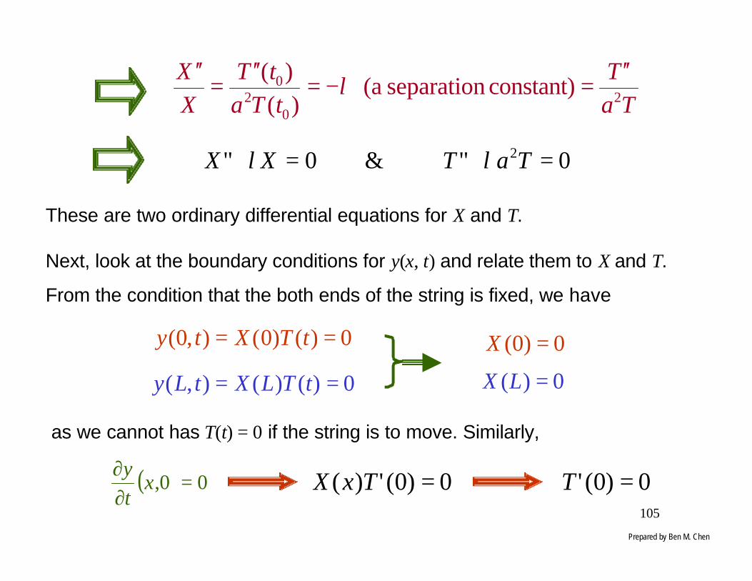
TaT

tTatT

XX

20

20 constant) separation(a

)(

)( ′′=−=

′′=

′′λ

0"&0" 2 =+=+ TaT XX λλ

These are two ordinary differential equations for X and T.

Next, look at the boundary conditions for y(x, t) and relate them to X and T.

From the condition that the both ends of the string is fixed, we have

0)()0(),0( == tTXty

0)()(),( == tTLXtLy

0)0( =X

0)( =LX

as we cannot has T(t) = 0 if the string is to move. Similarly,

( ) 00, =∂∂

xty

0)0(')( =TxX 0)0(' =T


106

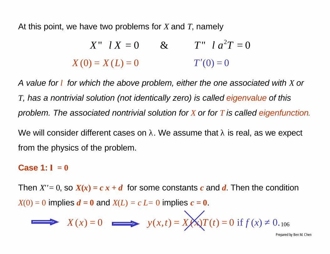
At this point, we have two problems for X and T, namely

0"&0" 2 =+=+ TaT XX λλ

0)()0( == LXX 0)0( =′T

A value for λ for which the above problem, either the one associated with X or

T, has a nontrivial solution (not identically zero) is called eigenvalue of this

problem. The associated nontrivial solution for X or for T is called eigenfunction.

We will consider different cases on λ. We assume that λ is real, as we expect

from the physics of the problem.

Case 1: λλ = 0

Then X′′= 0, so X(x) = c x + d for some constants c and d. Then the condition

X(0) = 0 implies d = 0 and X(L) = c L= 0 implies c = 0.

0)( =xX 0)()(),( == tTxXtxy if f (x) ≠ 0.Prepared by Ben M. Chen

107

Case 2: λλ < 0

For this case, we write λ = − k2 with k > 0. The equation for X is the given by

0" 2 =− XkX kxkx decexX −+=)(

0)0( =+= dcX dc −=

( ) )sinh(2)( kxceecxX kxkx =−= −

0)sinh(2)( == kLcLX 0== cd

because sinh(x) > 0 if x > 0. Thus,

solution.admissible an not is whichtTxXtxy 0)()(),( ==


108

Case 3: λλ >0

We can write λ = k2 with k > 0. Then

0" 2 =+ XkX )sin()cos()( kxdkxcxX +=

0)0( == cX )sin()( kxdxX =

0)sin()( == kLdLX

We cannot choose d = 0 as it will give a trivial solution again. Instead, we have

to let

0)sin( =kL ⋅⋅⋅== ,,,n nkL 321,π 2

222

Ln

kπ

λ ==

Corresponding to each positive integer n, we therefore have a solution for X:

( )

= x

Ln

dxX nn

πsin


109

Now look at the problem for T:

2

222

Ln

kπλ == ( ) 00;0

222

=′=+′′ T TL

anT

π

( )

+

= t

Lan

tL

antT

πβ

πα sincos

( ) 00cossin00

=⇒==

+

−=′

=

βπβππβππα

Lan

tL

anL

ant

Lan

Lan

Tt

( ) L,2,1,cos =

= nt

Lan

tT nn

πα

We now have, for each positive integer n, a function

( ) ( ) ( )

=

== t

Lan

xL

nAt

Lan

xL

ndtTxXtxy nnnnnn

ππππα cossincossin,

which satisfies wave equation and boundary conditions, but not initial position.Prepared by Ben M. Chen

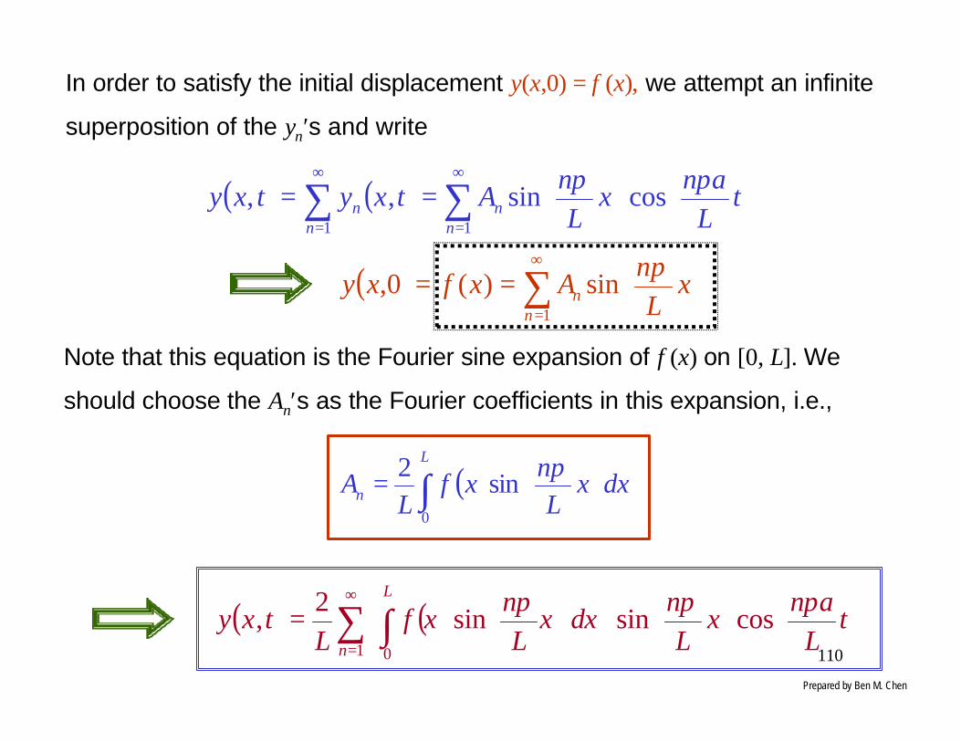
110

In order to satisfy the initial displacement y(x,0) = f (x), we attempt an infinite

superposition of the yn′s and write

( ) ( ) ∑∑∞

=

∞

=

==

11

cossin,,n

nn

n tL

anx

Ln

Atxytxyππ

( ) ∑∞

=

==

1

sin)(0,n

n xL

nAxfxy

π

Note that this equation is the Fourier sine expansion of f (x) on [0, L]. We

should choose the An′s as the Fourier coefficients in this expansion, i.e.,

( )∫

=

L

n dxxL

nxf

LA

0

sin2 π

( ) ( )

= ∑ ∫

∞

=

tL

anx

Ln

dL

nf

Ltxy

n

L ππξξπξ cossinsin2

,1 0


111

Example: Suppose that initially the string is picked up L/2 units at its center

point and then release from the rest.

0 LL/2

L/2 ( )

≤≤−≤≤

=LxL xL

Lx xxf

2/

2/0

( ) ( )

−+

=

= ∫ ∫∫

2/

0 /0

sinsin2

sin2 L L

xL

L

n dxxL

nxLdxx

Ln

xL

dxxL

nxf

LA

πππ

( )

−

−−

+

−= ∫∫

L

L

L

dxL

xnnL

LL

Lxn

nxLL

dxL

xnnLLxn

nLx

L 2/

2/

0

cos2

coscos02

2cos

2 ππ

ππ

ππ

ππ

−

+

+

−=

2sin

2cos

202sin

2cos

2

2222

LL

Lxn

nLn

nLL

Lxn

nLn

nL

L2 π

ππ

ππ

ππ

π

=

+

=

2sin

4

2sin

2sin

222

22 ππ

ππ

ππ

nn

LnnLn

nL

L= An


112

( )

= ∑

∞

= Latn

Lxnn

nL

txyn

ππππ

cossin2

sin14

,1

22

( )

=−=

+ 12 if 1

even is if 0

2sin 1 k- n

nnk

πNote that

( )( ) 1

22122 112

4,0 +

− −−

== nnn n

LAA

π

( ) ( )( )

( ) ( )

−

−

−−

= ∑∞

=

+

tL

anx

Ln

nL

txyn

n πππ

12cos

12sin

12

14,

12

1

2

The number λ = n2π2/L2 are eigenvalues, and the functions sin(nπx/L), or non-

zero multiple thereof, are eigenfunctions. The eigenvalues carry information

about the frequencies of the individual sine waves which are superimposed

to form the final solution.


113

0 0.5 10

0.5

1

1.5

2

t = 00 0.5 1

0

0.2

0.4

0.6

t = 10 0.5 1

-0.5

-0.4

-0.3

-0.2

-0.1

0

t = 2

0 0.5 1-1.5

-1

-0.5

0

t = 30 0.5 1

-0.8

-0.6

-0.4

-0.2

0

t = 40 0.5 1

0

0.1

0.2

0.3

t = 5

Simulation Results: L = ππ and a = 1

×π ×π

×π ×π×π

×π


114

Wave Equation with Zero Initial Displacement but Nonzero Velocity

Now let us consider the case in which the string is released from its horizontal

stretched position (zero initial displacement) but with a nonzero initial velocity.

The boundary value modeling this phenomenon is

2

22

2

2

xy

aty

∂∂=

∂∂

( ) ( ) 0,,0 == tLyty

( ) 00, =xy

( ) ( )xgxty =

∂∂

0,

0≥t

Lx ≤≤0

Lx ≤≤0

Lx ≤≤00≥t

Wave equation

Boundary conditions

Initial displacement

Initial velocity

Up to a point the analysis is the same as in the preceding problem. The only

difference between this problem and the previous one is that one would

have to choose An now to meet the initial velocity instead of initial position.Prepared by Ben M. Chen

115

)()(),( tTxXtxy =

As in the previous case, we set

to get

0"&0" 2 =+=+ TaT XX λλ0)()0( == LXX 0)0(0)0()( =⇒= TTxX

The problem for X is the same as that encountered previously, so the eigen-

values are

2

22

Ln π

λ =

For n = 1, 2, 3, ⋅ ⋅ ⋅ and corresponding eigenfunctions are

Now, however, we come to the difference between this problem and the

preceding one, i.e., the solution for T.


=

Lxn

dxX nn

πsin)(

116

Since we know the values of λ, the problem for T can be re-written as

( ) 00 ,02

222

==+′′ TTL

anT

π

The general solution of this differential equation for T is

( )

+

=

Latn

Latn

tT nnnπ

βπ

α sincos

( )

=⇒=⇒=

Latn

tTT nnn

πβα sin)(000

For each positive integer n, we now have

( )

=

=

Latn

Lxn

DLatn

Lxn

dtxy nnnn

ππππβ sinsinsinsin,

Each of these functions satisfies the wave equation, the boundary conditions,

and yn(x, 0) = 0, it in general does not satisfy the initial velocity condition.


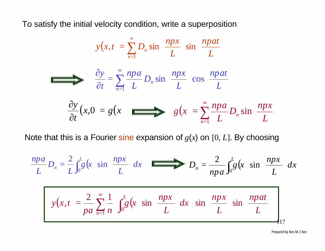
117

To satisfy the initial velocity condition, write a superposition

( ) ∑∞

=

=

1

sinsin,n

n Latn

Lxn

Dtxyππ

Note that this is a Fourier sine expansion of g(x) on [0, L]. By choosing

( ) ξπξ

ξπ

dL

ng

LD

Lan L

n

= ∫ sin

20

( ) ( )∑ ∫∞

=

=

10

sinsinsin12

,n

L

Latn

Lxn

dL

ng

natxy

ππξ

πξξ

π

∑∞

=

=

∂∂

1

cossinn

n Latn

Lxn

DL

anty πππ

( ) ( )xgxty =

∂∂

0, ( ) ∑∞

=

=

1

sinn

n Lxn

DL

anxg

ππ

( ) ξπξ

ξπ

dL

ng

anD

L

n

= ∫ sin

20


118

Example: We consider the same wave equation as in the preceding one but

with zero initial displacement and a initial velocity

( )

≤<≤≤

=

4L

40

0 Lx

Lxxxg

( )

−

=

=

∫∫ 4

cos44

sin sinsin2

22

24

00

ππ

ππ

ξπξξξπξξ nnLn

nL

dL

nd

Ln

gLL

( ) ∑∞

=

−

=

1232

2

sinsin4

cos4

1

4sin

12,

n Latn

Lxnn

nn

naL

txyππππ

ππ


119

The Wave Equation with Initial Displacement and Velocity

( )( ) ( ) ( )( ) ( )

( ) ( ) L)x (xgxty

L)x (xfxy

t tLyty

L, tx xy

aty

<<=∂∂

<<=>==

><<∂∂

=∂∂

0 0,

0 0,

0 0,,0

00 2

22

2

2

2

22

2

2

xy

aty

∂∂=

∂∂

( ) ( ) 0,,0 == tLyty

( ) ( )xfxy =0,

( ) 00, =∂∂

xty

Lx ≤≤0

0≥t

Lx ≤≤0

Lx ≤≤0

0≥t 2

22

2

2

xy

aty

∂∂=

∂∂

( ) ( ) 0,,0 == tLyty

( ) 00, =xy

( ) ( )xgxty =

∂∂

0,

0≥t

Lx ≤≤0

Lx ≤≤0

Lx ≤≤00≥t

+


120

Example: Consider the wave equation with usual boundary and with initial

displacement,

( )

≤≤≤≤

−=

LxL

Lx

xL

xxf

2

20

and initial velocity

( )

≤<≤≤

=LxL

Lxxxg

4

40

0

Then it follows from the previous examples, the solution to the above

problem is given by

( )

∑

∑∞

=

∞

=

−

+

=

1232

2

122

sinsin4

cos4

1

4sin

12

cossin2

sin14

,

n

n

Latn

Lxnn

nn

naL

Latn

Lxnn

nL

txy

ππππππ

ππππ


121

Simulation Results: L = ππ and a = 1

0 0.5 10

0.2

0.4

0.6

0.8

t = 10 0.5 1

-0.5

-0.4

-0.3

-0.2

-0.1

0

t = 2

0 0.5 1-1.5

-1

-0.5

0

t = 30 0.5 1

-1

-0.8

-0.6

-0.4

-0.2

0

t = 40 0.5 1

0

0.1

0.2

0.3

t = 5

0 0.5 10

0.5

1

1.5

2

t = 0


122

Fourier Series Solution of the Heat Equation

The Ends of the Bar Kept at Zero Temperature: We want to determine the

temperature distribution u(x,t) in a thin homogeneous bar of length L, given

the initial temperature distribution throughout the bar at time t = 0, if the ends

are maintained at zero temperature for all time.

The boundary value problem is

( )

( ) ( ) ( )( ) ( ) )0( 0,

0 0,,0

00 2

22

Lxxfxu

t tLutu

L, txxu

atu

<<=>==

><<∂∂

=∂∂ Heat Equation

Boundary Conditions

Initial Temperature

The procedure that we are going to use to solve the above problem is precisely

the same as the one in solving the wave equation. All the dirty works were done

already. The rest is pretty simple. Prepared by Ben M. Chen

123

We will apply the separation of variables method and seek a solution

)()(),( tTxXtxu =

2

22

xu

atu

∂∂

=∂∂

)()()()( 2 tTxXatTxX ′′=′)(

)(

)(

)( 2

xXxX

atTtT ′′

=′

Since x and t are independent variables, both sides of this equation must be

equal to the same constant.

λ−==XX

TaT "'2 0 and 0" 2 =+=+ Ta T'XX λλ

0)0(0)()0(0),0( =⇒=⇒= XtTXtu

0)(0)()(0),( =⇒=⇒= LXtTLXtLu

Unlike the wave equation, this equation for T is of first order, with no boundary

condition.

0&0)()0(,0 2 =+′===+′′ TaTLXXXX λλ


124

The boundary value problem for X, however, is identical with that encountered

with the wave equation, so we have eigenvalues and eigenfunctions

2

22

Ln

ë n

π= ( ) L

xndxX nn

= π

sin&

With the values we have for λ, the differential equation for T is

0'2

222

=+ TLna

Tπ

Each un(x,t) satisfies the heat equation and both boundary conditions, but in

general, none of them will satisfy the initial condition, i.e.,

( ) ( ) )0( 0, Lx xfxu <<=

2222 /)( Ltannn etT πα −=

2222 /sin)()(),( Ltannnnn e

Lxn

AtTxXtxu ππ −

==


125

Thus, we should attempt an infinite superposition

∑∑∞

=

−∞

=

==

1

/

1

2222

sin),(),(n

Ltann

nn e

Lxn

Atxutxu ππ

This is the Fourier series expansion of f on [0, L]. Hence, choose the An′s as

the Fourier coefficients:

ξπξ

ξπ

dL

nf

Ldx

Lxn

xfL

ALL

n

=

= ∫∫ sin)(

2sin)(

200

2222 /

10

sinsin)(2

),( Ltan

n

Le

Lxn

dL

nf

Ltxu ππ

ξπξ

ξ −∞

=∑ ∫

=

∑∞

=

==

1

sin)()0,(n

n Lxn

Axfxuπ


Documents

Ben M. Chen Associate Professor Office: E4-6-7 Phone: 874 ...uav.ece.nus.edu.sg/~bmchen/courses/ee2462-ppt.pdf · ... solution of Bessel′s equation in terms of Gamma ... wave equation;