Embed Size (px)
Citation preview
Unclassified NEA/CSNI/R(2011)4 Organisation de Coopération et de Développement Économiques Organisation for Economic Co-operation and Development 28-Mar-2011 ___________________________________________________________________________________________
English text only NUCLEAR ENERGY AGENCY COMMITTEE ON THE SAFETY OF NUCLEAR INSTALLATIONS
BEMUSE Phase VI Report Status report on the area, classification of the methods, conclusions and recommendations
JT03299065
Document complet disponible sur OLIS dans son format d'origine Complete document available on OLIS in its original format
NE
A/C
SNI/R
(2011)4 U
nclassified
English text only
Cancels & replaces the same document of 11 March 2011

NEA/CSNI/R(2011)4
2
ORGANISATION FOR ECONOMIC CO-OPERATION AND DEVELOPMENT The OECD is a unique forum where the governments of 34 democracies work together to address the economic, social and
environmental challenges of globalisation. The OECD is also at the forefront of efforts to understand and to help governments respond to new developments and concerns, such as corporate governance, the information economy and the challenges of an ageing population. The Organisation provides a setting where governments can compare policy experiences, seek answers to common problems, identify good practice and work to co-ordinate domestic and international policies.
The OECD member countries are: Australia, Austria, Belgium, Canada, Chile, the Czech Republic, Denmark, Estonia, Finland, France, Germany, Greece, Hungary, Iceland, Ireland, Israel, Italy, Japan, Korea, Luxembourg, Mexico, the Netherlands, New Zealand, Norway, Poland, Portugal, the Slovak Republic, Slovenia, Spain, Sweden, Switzerland, Turkey, the United Kingdom and the United States. The European Commission takes part in the work of the OECD.
OECD Publishing disseminates widely the results of the Organisation’s statistics gathering and research on economic, social and environmental issues, as well as the conventions, guidelines and standards agreed by its members.
This work is published on the responsibility of the Secretary-General of the OECD. The opinions expressed and arguments employed herein do not necessarily reflect the official
views of the Organisation or of the governments of its member countries.
NUCLEAR ENERGY AGENCY The OECD Nuclear Energy Agency (NEA) was established on 1st February 1958 under the name of the OEEC European Nuclear
Energy Agency. It received its present designation on 20th April 1972, when Japan became its first non-European full member. NEA membership today consists of 29 OECD member countries: Australia, Austria, Belgium, Canada, the Czech Republic, Denmark, Finland, France, Germany, Greece, Hungary, Iceland, Ireland, Italy, Japan, Korea, Luxembourg, Mexico, the Netherlands, Norway, Poland, Portugal, the Slovak Republic, Spain, Sweden, Switzerland, Turkey, the United Kingdom and the United States. The European Commission also takes part in the work of the Agency.
The mission of the NEA is: – to assist its member countries in maintaining and further developing, through international co-operation, the scientific,
technological and legal bases required for a safe, environmentally friendly and economical use of nuclear energy for peaceful purposes, as well as
– to provide authoritative assessments and to forge common understandings on key issues, as input to government decisions on nuclear energy policy and to broader OECD policy analyses in areas such as energy and sustainable development.
Specific areas of competence of the NEA include safety and regulation of nuclear activities, radioactive waste management, radiological protection, nuclear science, economic and technical analyses of the nuclear fuel cycle, nuclear law and liability, and public information.
The NEA Data Bank provides nuclear data and computer program services for participating countries. In these and related tasks, the NEA works in close collaboration with the International Atomic Energy Agency in Vienna, with which it has a Co-operation Agreement, as well as with other international organisations in the nuclear field. Corrigenda to OECD publications may be found online at: www.oecd.org/publishing/corrigenda. © OECD 2011 You can copy, download or print OECD content for your own use, and you can include excerpts from OECD publications, databases and multimedia products in your own documents, presentations, blogs, websites and teaching materials, provided that suitable acknowledgment of OECD as source and copyright owner is given. All requests for public or commercial use and translation rights should be submitted to [email protected]. Requests for permission to photocopy portions of this material for public or commercial use shall be addressed directly to the Copyright Clearance Center (CCC) at [email protected] or the Centre français d'exploitation du droit de copie (CFC) [email protected].

NEA/CSNI/R(2011)4
3
COMMITTEE ON THE SAFETY OF NUCLEAR INSTALLATIONS
The Committee on the Safety of Nuclear Installations (CSNI) shall be responsible for the activities of the Agency that support maintaining and advancing the scientific and technical knowledge base of the safety of nuclear installations, with the aim of implementing the NEA Strategic Plan for 2011-2016 and the Joint CSNI/CNRA Strategic Plan and Mandates for 2011-2016 in its field of competence.
The Committee shall constitute a forum for the exchange of technical information and for collaboration between organisations, which can contribute, from their respective backgrounds in research, development and engineering, to its activities. It shall have regard to the exchange of information between member countries and safety R&D programmes of various sizes in order to keep all member countries involved in and abreast of developments in technical safety matters.
The Committee shall review the state of knowledge on important topics of nuclear safety science and techniques and of safety assessments, and ensure that operating experience is appropriately accounted for in its activities. It shall initiate and conduct programmes identified by these reviews and assessments in order to overcome discrepancies develop improvements and reach consensus on technical issues of common interest. It shall promote the co-ordination of work in different member countries that serve to maintain and enhance competence in nuclear safety matters, including the establishment of joint undertakings, and shall assist in the feedback of the results to participating organisations. The Committee shall ensure that valuable end-products of the technical reviews and analyses are produced and available to members in a timely manner.
The Committee shall focus primarily on the safety aspects of existing power reactors, other nuclear installations and the construction of new power reactors; it shall also consider the safety implications of scientific and technical developments of future reactor designs.
The Committee shall organise its own activities. Furthermore, it shall examine any other matters referred to it by the Steering Committee. It may sponsor specialist meetings and technical working groups to further its objectives. In implementing its programme the Committee shall establish co-operative mechanisms with the Committee on Nuclear Regulatory Activities in order to work with that Committee on matters of common interest, avoiding unnecessary duplications.
The Committee shall also co-operate with the Committee on Radiation Protection and Public Health, the Radioactive Waste Management Committee, the Committee for Technical and Economic Studies on Nuclear Energy Development and the Fuel Cycle and the Nuclear Science Committee on matters of common interest.

NEA/CSNI/R(2011)4
4
Coordinator: H. Glaeser (GRS, Germany).
Contributors: Appendix 1: P. Bazin (CEA, France);
Appendix 2: J. Baccou, E. Chojnacki, S. Destercke (IRSN, France).
Coordinators of the previous Phases of BEMUSE:
Phase I: Presentation “a priori” of the uncertainty evaluation methodology to be used by the
participants; E. Chojnacki, J.-C. Micaelli (IRSN, France).
Phase II: Re-analysis of the ISP-13 exercise, post-test analysis of the LOFT L2-5 test calculation; A.
Petruzzi, F. D’Auria (Università di Pisa, Italy).
Phase III: Uncertainty evaluation of the L2-5 test calculations, first conclusions on the methods and
suggestions for improvement; A. de Crécy, P. Bazin (CEA, France).
Phase IV: Best-estimate analysis of a NPP-LBLOCA; F. Reventós, M. Pérez, L. Batet, R. Pericas
(Universitat Politècnica de Catalunya, Barcelona, Spain).
Phase V: Sensitivity analysis and uncertainty evaluation for the NPP LBLOCA, with or without
methodology improvements resulting from phase III; F. Reventós, L. Batet, M. Pérez
(Universitat Politècnica de Catalunya, Barcelona, Spain).

NEA/CSNI/R(2011)4
5
Acknowledgement
This report uses information and material produced during the previous phases of the BEMUSE Programme. The author likes to acknowledge the big amount of work produced during these phases.
This report was extensively reviewed by participants of BEMUSE as well as WGAMA members. I gratefully acknowledge their very valuable and constructive comments, particularly from: A. de Crécy and P. Bazin from CEA, I. Tóth and A. Guba from AEKI, F. D’Auria from University Pisa, E. Chojnacki from IRSN, D.-Y. Oh from KINS, R. Pernica and M. Kyncl from NRI, S. Borisov from EDO “Gidropress”, S. Bajorek from USNRC, A. Bucalossi from European Commission Joint Research Centre, A. Amri from OECD-NEA, T. Skorek from GRS.

NEA/CSNI/R(2011)4
6
NEA/CSNI/R(2011)4
7
TABLE OF CONTENTS
EXECUTIVE SUMMARY ............................................................................................................................ 9
INTRODUCTION ........................................................................................................................................ 13
1.1 Historical Background .................................................................................................................... 13 1.2 Uncertainty Methods Study (UMS) ................................................................................................ 15 1.3 BEMUSE Programme .................................................................................................................... 16
1.3.1 Main steps of BEMUSE............................................................................................................ 16 1.3.2 Objectives of BEMUSE ............................................................................................................ 17
2. BEMUSE PHASE I ............................................................................................................................... 19
2.1 Participants ..................................................................................................................................... 19 2.2 Main steps of a statistical method .................................................................................................. 19 2.3 Main steps of the CIAU method ..................................................................................................... 20
3.BEMUSE PHASE II .................................................................................................................................. 21
3.1 Objectives ....................................................................................................................................... 21 3.2 Participants ..................................................................................................................................... 21 3.3 Selected Results .............................................................................................................................. 22 3.4 Summary of phase II ...................................................................................................................... 26
4. BEMUSE PHASE III ......................................................................................................................... 27
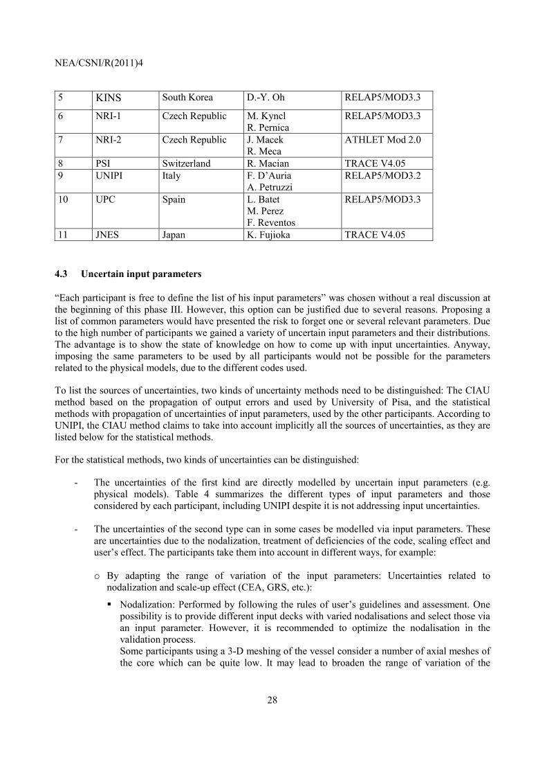
4.1 Objectives and scope ...................................................................................................................... 27 4.2 Participants ..................................................................................................................................... 27 4.3 Uncertain input parameters............................................................................................................. 28 4.4 Main results ................................................................................................................................... 30
4.4.1 Results of reference calculations............................................................................................... 30 4.4.2 Results of uncertainty analysis .................................................................................................. 31 4.4.3 Results of sensitivity or influence analysis ............................................................................... 33
4.5 Additional investigations using statistical methods........................................................................ 37 4.5.1 Investigation of statistical convergence of tolerance limits by increasing the number of code runs .................................................................................................................................................. 38 4.5.2 Modifying the type of probability distribution and truncation.................................................. 40
4.6 Conclusions of phase III ................................................................................................................. 41
5. BEMUSE PHASE IV ........................................................................................................................... 43
6. BEMUSE PHASE V ................................................................................................................................. 47
6.1 Objectives of phase V ..................................................................................................................... 47 6.2 Participants ..................................................................................................................................... 47 6.3 Specific working steps compared with phase III ............................................................................ 47 6.4 Treatment of failed code runs ......................................................................................................... 52 6.5 Main results .................................................................................................................................... 53

NEA/CSNI/R(2011)4
8
6.5.1 Results of reference calculations............................................................................................... 53 6.5.2 Results of uncertainty analysis .................................................................................................. 55 6.5.3 Results of sensitivity analysis ................................................................................................... 66
6.6 Conclusions of Phase V .................................................................................................................. 69
7. CONCLUSIONS AND RECOMMENDATIONS ................................................................................... 71
7.1 Uncertainty methods and computer codes used ............................................................................. 71 7.2 Number of uncertain input parameters, determination of distributions and selection of values from their distributions....................................................................................................................................... 72 7.3 Uncertainty results .......................................................................................................................... 73 7.4 Influence or sensitivity results ........................................................................................................ 74 7.5 Treatment of failed runs ................................................................................................................. 75 7.6 Statistical convergence of tolerance limits ..................................................................................... 75 7.7 Lessons learned .............................................................................................................................. 76 7.8 General remarks ............................................................................................................................. 77
REFERENCES ............................................................................................................................................. 79
ABBREVIATIONS ..................................................................................................................................... 81
APPENDIX 1: FURTHER EVALUATION OF RESULTS FROM BEMUSE PHASE V ........................ 83
A1-1 First PCT ................................................................................................................................... 83 A1-2 Second PCT .............................................................................................................................. 87 A1-3 Maximum PCT ......................................................................................................................... 90 A1-4 Summary ................................................................................................................................... 92
APPENDIX 2: DESCRIPTION OF EVALUATION AND SYNTHESIS OF MULTIPLE SOURCES OF INFORMATION AND FURTHER APPLICATION TO AN ANALYSIS OF BEMUSE PHASE III AND PHASE V COMPUTER CODE RESULTS ................................................................................................. 93
Introduction ............................................................................................................................................... 93 A2-1 Evaluation and synthesis methods ............................................................................................ 93
A2-1.1 Information representation .................................................................................................... 94 A2-1.2 Information evaluation .......................................................................................................... 95 A2-1.3 Information synthesis ............................................................................................................ 97
A2-2 Application to the analysis of BEMUSE phase III results ........................................................ 98 A2-2.1 Considered variables ............................................................................................................. 98
A2-3 Application to the analysis of BEMUSE phase V results ....................................................... 105 A2-3.1 Considered variables .............................................................................................................. 105
A2-3.2 Modelling ............................................................................................................................ 105 A2-3.3 Source evaluation ................................................................................................................ 106 A2-3.4 Information synthesis .......................................................................................................... 107 A2-3.4.3 Synthesis of the information with respect to uncertainty method ................................... 119 A2-3.5 Conclusions ......................................................................................................................... 122
A2-4 References ............................................................................................................................... 122
NEA/CSNI/R(2011)4
9
EXECUTIVE SUMMARY
Background
Since nuclear energy was first used to produce electricity in the 1950s, the evaluation of nuclear power plant performance during accidental transient conditions has been the main issue in thermal-hydraulic safety research worldwide. A huge amount of experimental data have been made available from very simple loops (Basic Test Facilities and Separate Effect Test Facilities) and from very complex Integral Test Facilities, simulating all the relevant parts of a Light Water Reactor (LWR). Sophisticated computer codes such as ATHLET, CATHARE, RELAP, TRAC and TRACE have also been developed, mainly in Europe and United States, and are now widely used. Such codes can calculate time trends of many variables of interest during transients in LWRs. The reliability of the predictions cannot be assessed directly due to the lack of suitable measurements in plants. The capabilities of the codes can consequently only be assessed by comparison of calculation results with experimental data recorded in small scale facilities. To evaluate the applicability of a code in predicting a plant situation, it is necessary to check, at least, that experimental data used for qualifying the codes are representative of phenomena expected in the plant and, subsequently that codes can qualitatively and quantitatively reproduce such data. Furthermore, the best-estimate character of the software quoted above involves adding an evaluation of the uncertainties of calculation results of the plant transient. Another issue of interest is sensitivity analysis, which provides additional information on the results of uncertainty analysis.
In this context, the BEMUSE (Best Estimate Methods – Uncertainty and Sensitivity Evaluation) Programme – promoted by the Working Group on Analysis and Management of Accidents (WGAMA) and endorsed by the Committee on the Safety of Nuclear Installations (CSNI) – represents an important step towards reliable application of high-quality best-estimate and uncertainty and sensitivity evaluation methods.
The programme was divided into two main steps, each one consisting of three phases. The first step is to perform an uncertainty and sensitivity analysis related to the LOFT L2-5 test, and the second step is to perform the same analysis for a Nuclear Power Plant (NPP) Large Break Loss of Coolant Accident (LBLOCA). The programme started in January 2004.
• First step (Phases 1, 2 and 3):
- Phase I: Presentation “a priori” of the uncertainty evaluation methodology to be used by the participants.
- Phase II: Re-analysis of the ISP-13 exercise, post-test analysis of the LOFT L2-5 large cold leg break test calculation.
- Phase III: Uncertainty evaluation of the L2-5 test calculations, first conclusions on the methods and suggestions for improvement.

NEA/CSNI/R(2011)4
10
• Second step (Phases IV, V and VI):
- Phase IV: Best-estimate analysis of a NPP-LBLOCA.
- Phase V: Sensitivity analysis and uncertainty evaluation for the NPP. LBLOCA, with or without methodology improvements resulting from Phase III.
- Phase VI: Status report on the area, classification of the methods, conclusions and recommendations.
As indicated in the last point, this report on BEMUSE Phase VI summarises the main results from the previous phases of the BEMUSE Programme, gives information about the applied methods and summarizes conclusions and recommendations from the whole Programme. Objectives of the programme
The BEMUSE programme is focused on the application of uncertainty methodologies to LB-LOCA scenarios. The main goals of the programme are:
- To evaluate the practicability, quality and reliability of Best Estimate methods including
uncertainty evaluations in applications relevant to nuclear reactor safety - To develop a common understanding in this domain - To promote/facilitate the use of these methods by the regulatory bodies and the industry.
Operational objectives include an assessment of the applicability of best estimate and uncertainty and sensitivity methods to integral tests and their use in reactor applications. The justification for such an activity is that some uncertainty methods applied to BE codes exist and are used in research organisations, by vendors, technical safety organisations and regulatory authorities. Over the last years, the increased use of BE codes and uncertainty and sensitivity evaluation for Design Basis Accident (DBA), by itself, shows the safety significance of the proposed activity. Uncertainty methods are used worldwide in licensing of loss of coolant accidents for power uprates of existing plants, for new reactors and new reactor developments. End users for the results are expected to be industry, safety authorities and technical safety organisations.
Used methods
Two classes of uncertainty methods can be distinguished. One propagates “input uncertainties” and the other one extrapolates “output uncertainties”. The main characteristics of the methods based upon the propagation of input uncertainties is to assign probability distributions for these input uncertainties, and sample out of these distributions values for each code calculation to be performed. The number of code calculations is independent of the number of input uncertainties, but is only dependent on the defined probability content (percentile) and confidence level. The number of calculations is given by Wilks’ formula. By performing code calculations using variations of the values of the uncertain input parameters, and consequently calculating results dependent on these variations, the uncertainties are propagated in the calculations up to the results. Uncertainties are due to imprecise knowledge and the approximations of the computer codes simulating thermal-hydraulic physical behaviour.

NEA/CSNI/R(2011)4
11
The methods based upon extrapolation of output uncertainties need available relevant experimental data, and extrapolate the differences between code calculations and experimental data at reactor scale. The main difference of this method compared with statistical methods is that there is no need to select a reasonable number of uncertain input parameters and to provide uncertainty ranges (or distribution functions) for each of these variables. The determination of uncertainty is only on the level of calculation results due to the extrapolation of deviations between measured data and calculation results. The two principles have advantages and drawbacks. The probabilistic methods are associated with order statistics. The method needs to select a reasonable number of variables and associated range of variations and possibly distribution functions for each one. Selection of parameters and their distribution must be justified. Uncertainty propagation occurs through calculations of the code under investigation. The “extrapolation on the outputs” method has no formal analytical procedure to derive uncertainties, and needs to have “relevant experimental data” available. In addition, the sources of error cannot be derived as result of application of the method. The method seeks to avoid engineering judgement as much as possible.
In BEMUSE phases III and V, the majority of participants used the probabilistic approach, associated with Wilks’ formula. Only University of Pisa used its method extrapolating output uncertainties. This method is called the CIAU method, Code with (the capability of) Internal Assessment of Uncertainty. Conclusions and recommendations
The methods used in this activity are considered to be mature for application, including licensing processes. Lessons learned for a proper application of the statistical method are listed as result of the performed exercise. Differences are observed in the application of the methods, consequently results of uncertainty analysis of the same task lead to different results. These differences raise concerns about the validity of the results obtained when applying uncertainty methods to system analysis codes. The differences may stem from the application of different codes and uncertainty methods. In addition, differences between applications of statistical methods may mainly be due to different input uncertainties, their ranges and distributions. Differences between CIAU applications may stem from different data bases used for the analysis. However, as it was shown by BEMUSE phases III and V, significant differences were observed between the base or reference calculation results. Furthermore, differences were seen in the results using the same values of single input parameter variations in BEMUSE phases II and IV.
When a conservative safety analysis method is used, it is claimed that all uncertainties which are considered by an uncertainty analysis are bounded by conservative assumptions. Differences in calculation results of conservative codes would also be seen, due to the user effect such as different nodalisation and code options, like for best estimate codes used in the BEMUSE programme. Difference of code calculation results have been observed for a long time, and have been experienced in all International Standard Problems where participants calculated the same experiment or a reactor event. The main reason is that the user of a computer code has a big influence on how a code is used. The objective of an uncertainty analysis is to quantify the uncertainties of a code result. An uncertainty analysis cannot compensate for code deficiencies. Therefore, necessary pre-condition is that the code is suitable to calculate the scenario under investigation.
A user effect can also be seen in applications of uncertainty methods, like in the BEMUSE programme. In uncertainty analysis, the emphasis is on the quantification of a lack of precise knowledge by defining appropriate uncertainty ranges of input parameters, which could not be achieved in all cases in BEMUSE. For example, some participants specified too narrow uncertainty ranges for important input uncertainties based on expert judgement, and not on sufficient code validation experience. Therefore, skill, experience and knowledge of the users about the applied suitable computer code as well as the used uncertainty method are important for the quality of the results.
NEA/CSNI/R(2011)4
12
Instead of emphasising too much an appropriate number of calculations to be performed when applying the statistical method, one should concentrate first on the basis or reference calculation. However, an increased number of calculations may be advisable because it decreases the dispersion of the tolerance limits. Secondly, it is very important to include influential parameters and provide distributions of uncertain input parameters, mainly their ranges. These assumptions must be well justified. An important basis to determine code model uncertainties is the experience from code validation. This is mainly provided by experts performing the validation. Appropriate experimental data are needed. More effort, specific procedures and judgement should be focused on the determination of input uncertainties.
This last point is an issue for recommendation for further work. Especially, the method used to select and quantify computer code model uncertainties and to compare their effects on the uncertainty of the results could be studied in a future common international investigation using different computer codes. That may be performed based on one experiment. Possibly approaches can be tested to derive these uncertainties by comparing calculation results and experimental data. Other areas are selection of nodalisation and code options. This issue on improving the reference calculations among participants is fundamental in order to obtain more common bands of uncertainties of the results.

NEA/CSNI/R(2011)4
13
INTRODUCTION
The BEMUSE (Best Estimate Methods, Uncertainty and Sensitivity Evaluation) Programme has been promoted by the Working Group on Accident Management and Analysis (GAMA) and endorsed by the Committee on the Safety of Nuclear Installations (CSNI). The objectives of this programme were to evaluate the practicability, quality and reliability of best-estimate methods including uncertainty evaluations in applications relevant to nuclear reactor safety, to develop common understanding and to promote/facilitate their use by the regulatory bodies and the industry. The programme focused on the applications of uncertainty methodologies to large break LOCA (Loss of Coolant Accident) in PWR (Pressurized Water Reactor).
Uncertainties of code calculation results come from approximations of the balance or conservation equations in system thermal-hydraulic computer codes. Not all interactions between steam and liquid are included. Lacking information has to be supplied by the code users. Averaging over a cross section scale is another approximation whereas velocity profiles occur in reality, for example. These uncertainties are expressed by uncertainties of models in the code. Other uncertainties may be due to imprecise knowledge of initial and boundary conditions, not exactly known flow paths, like bypass flows in the reactor vessel, fuel parameters, and so on.
1.1 Historical Background
The first uncertainty analysis was performed with the CSAU methodology [1]. The method was demonstrated in 1989 using the TRAC-PF1 code for a large break loss of coolant accident (LB-LOCA). The main issues of uncertainty analysis were already described: Selection of the uncertain input parameters, determination of their range of variation and propagation of these input uncertainties. The number of input parameters was limited to less than 10 via a phenomena identification and ranking process. Values were assigned to the input parameters inside their range of variation and roughly 100 TRAC calculations were performed by shifting the input parameters one by one, two by two, etc. according to these levels. The obtained values of the outputs were used to build a polynomial response surface. A large number of Monte-Carlo histories, typically 50000, were then performed with the response surface to estimate the desired percentiles of the outputs. This method can be seen as a mixing between a deterministic approach during the building of the response surface and a statistical one with the Monte-Carlo histories. In 1994, GRS proposed a fully statistical method [2]. It is based on the use of Wilks’ formula [3] to determine the number of code runs needed to obtain a given tolerance limit with a given confidence level. Unlike the CSAU, this number of code runs is independent of the number of input parameters and all the input parameters are sampled simultaneously. This method is presently largely used in research and licensing, as it was for phases III and V of BEMUSE.

NEA/CSNI/R(2011)4
14
At the same time, UNIPI proposed another method, the UMAE, based on the extrapolation of the code-experiment differences on the outputs, determined via a large experimental database [4]. This method has been completed in 2000 by the CIAU [5], used by UNIPI in licensing and for BEMUSE.
The first proposal to perform uncertainty analysis in licensing applications was initiated by the US Nuclear Regulatory Commission in the year 1989. The USA Code of Federal Regulations (CFR) 10 CFR 50.46 [6], for example, allows either to use a “best estimate” (BE) code plus identification and quantification of uncertainties, or the conservative option using conservative computer code models listed in Appendix K of the CFR. However, when using a best estimate computer code, it is required that uncertainties have to be identified and assessed so that the uncertainty in the calculated results can be estimated.
A high level of probability has to be applied that acceptance criteria would not be exceeded. That high level of probability is specified in the US NRC Regulatory Guide 1.157 to 95% or more [7]. Regulatory Guide 1.157 described the uncertainties to be considered for loss of coolant accidents (LOCA). Other events that must be considered in the safety analyses do not require a complete uncertainty analysis according to NRC Guide 1.203 [8]. In most cases “suitably conservative” input parameters should be used.
An IAEA Safety Report Series No. 23: “Accident analysis for Nuclear Power Plants”, issued in the year 2002, recommends sensitivity and uncertainty analysis if best estimate codes are used in licensing analysis [9]. A comprehensive overview about uncertainty methods can be found in the IAEA Safety Report Series No. 52, „Best Estimate Safety Analysis for Nuclear Power Plants: Uncertainty Evaluation“, issued in 2008 [10].
An IAEA Safety Guide SSG-2 “Deterministic Safety Analysis for Nuclear Power Plants”, published in December 2009 [11], provides harmonized guidance to designers, operators, regulators and providers of technical support on deterministic safety analysis for nuclear power plants. Three ways of analyzing anticipated operational occurrences and design basis accidents to demonstrate that the safety requirements are met, are currently used to support applications for licensing:
1. Use of conservative computer codes with conservative initial and boundary conditions (conservative analysis);
2. Use of best estimate computer codes combined with conservative initial and boundary conditions (combined analysis);
3. Use of best estimate computer codes with conservative and/or realistic input data but coupled with an evaluation of the uncertainties in the calculation results, with account taken of both the uncertainties in the input data and the uncertainties associated with the models in the best estimate computer code (best estimate analysis). The result, which reflects conservative choice but has a quantified level of uncertainty, is used in the safety evaluation.
The Safety Guide SSG-2 states that the use of best estimate analysis together with an evaluation of the uncertainties is increasing. Accordingly, emphasis is given to the third way to perform safety analysis. With regard to that approach, “it is common practice to require that assurance be provided of a 95% or greater probability that the applicable acceptance criteria for a plant will not be exceeded.” “Techniques may be applied that use additional confidence levels, for example, 95% confidence levels, with account taken of the possible sampling error due to the fact that a limited number of calculations have been performed.”
Nowadays, Best Estimate Plus Uncertainty Methods (BEPU) are extensively used worldwide in licensing of LOCAs (USA, Brazil, Korea, Netherlands, etc.) or significant activities are developed for a future use in licensing (Canada, Czech Republic, France, Japan, etc.). CSAU is often used, but more as a general framework for performing an uncertainty analysis including the use of a Phenomena Identification and
NEA/CSNI/R(2011)4
15
Ranking Table (PIRT) to limit the number of considered input parameters associated with the use of other statistical methods than that explained in the demonstration case [1]. Among these statistical methods, Wilks’ formula, used in the GRS method, is very often applied in research and in safety analysis in licensing applications. The UNIPI method has also been applied in licensing. For example, it was used in Brazil for the Angra-2 NPP licensing to verify the vendor’s method.
Even for the methods based on propagation of input uncertainties (CSAU and GRS), there is not yet a complete consensus about some questions. One can quote for example for these methods: Number of code runs, of input parameters, choice of these input parameters, determination of their range of variation, etc. Therefore, the BEMUSE programme was initiated, and especially the phases devoted to uncertainty and sensitivity analyses such as phases 3 and 5, provide an opportunity to gain insight in these different approaches, in different performances of codes and different analysts working on the same task.
1.2 Uncertainty Methods Study (UMS)
A former CSNI activity connected with uncertainty was the Uncertainty Method Study (UMS) which started in the year 1996 [12]. In this programme five different uncertainty methodologies were applied on a small break loss of coolant accident on the Japanese LSTF test facility. The calculations were performed for LSTF Test SB-CL-18, a 5% cold leg break, loss of off-site power and no high pressure ECC injection. LSTF has a volume scale of 1:48. Accumulators started ECC injection into the cold legs below 4.51 MPa, the low pressure ECC injection started below 1.29 MPa. The objectives of the Study were:
• A step by step comparison of five different methods.
• A comparison of the uncertainties predicted by different methods and the results of the experiment.
• To identify and explain the discrepancies between predicted uncertainties.
• To prove the suitability of these methods for quantifying uncertainties with best-estimate codes, in this particular application.
Four of the five involved uncertainty methods are based on a propagation of uncertainties through the computer code and one uncertainty method is based on accuracy extrapolation, i.e. the University of Pisa method UMAE (Uncertainty Method based on Accuracy Extrapolation). The principle of an uncertainty propagation method is to evaluate the uncertainty sources attached to the input data and physical models used by the code, and to propagate them by performing code calculations varying the input uncertainties according to their ranges and distributions. Among the uncertainty propagation methods, three methods are statistical (the ENUSA, GRS and IRSN methods), essentially following the GRS method, and the AEAT (Atomic Energy Authority Technology) method quantifies ranges and it is up to the analyst to combine values out of these ranges without using statistics.
UMS was the first international investigation to a small break LOCA. Five uncertainty analysis methods were compared. Approximately 340 runs modelling LSTF SB-CL-18 were performed. Uncertainty ranges were calculated that bound the data of the experiment. Small differences between the predictions of uncertainty ranges were obtained for pressure and primary mass. Significant differences were calculated for uncertainty ranges of peak cladding temperature of the hot rod. These differences came from a combination of the method used, the completeness of the identification and selection of uncertainties or relevant thermal-hydraulic aspects. For the Pisa method was the optimisation of the nodalisation and

NEA/CSNI/R(2011)4
16
possibly the different number of experiments used important for the differences between applications of two different codes. Five experiments with CATHARE were used, and 10 with RELAP. The main reasons for differences of the uncertainty propagation methods were the underlying accuracy of the reference calculation and the representation of the LSTF facility used, as well as the ranges of the input uncertainties, like uncertainty ranges or probability distributions. It follows that it is very important how the methods are applied.
1.3 BEMUSE Programme
1.3.1 Main steps of BEMUSE
The programme was divided into two main steps, each one consisting of three phases. The first step is to perform an uncertainty and sensitivity analysis related to the LOFT L2-5 test, and the second step is to perform the same analysis for a Nuclear Power Plant (NPP) Large Break Loss of Coolant Accident (LBLOCA). The programme started in January 2004.
• First step (Phases I, II and III):
- Phase I: Presentation “a priori” of the uncertainty evaluation methodology to be used by the participants (lead organization: IRSN).
- Phase II: Re-analysis of the ISP-13 exercise, post-test analysis of the LOFT L2-5 large cold leg break test calculation (lead organization: University of Pisa).
- Phase III: Uncertainty evaluation of the L2-5 test calculations, first conclusions on the methods and suggestions for improvement (lead organization: CEA).
• Second step (Phases IV, V and VI):
- Phase IV: Best-estimate analysis of a NPP-LBLOCA (lead organization: UPC Barcelona).
- Phase V: Sensitivity analysis and uncertainty evaluation for the NPP LBLOCA, with or without methodology improvements resulting from Phase III (lead organization: UPC Barcelona).
- Phase VI: Status report on the area, classification of the methods, conclusions and recommendations (lead organization: GRS).
As indicated in the last point, this report on BEMUSE Phase VI summarises the main results from the previous phases of the BEMUSE Programme, gives some information about the applied methods and summarizes conclusions and recommendations from the whole Programme. One new evaluation of results from phase V, the Zion Nuclear Power Plant is included in Appendix 1. A different approach to evaluate results of phase III, the uncertainty analyses of LOFT L2-5 post-test calculations, and phase V are included in Appendix 2.

NEA/CSNI/R(2011)4
17
1.3.2 Objectives of BEMUSE
The high-level objectives of the work are:
- To evaluate the practicability, quality and reliability of Best-Estimate (BE) methods including uncertainty and sensitivity evaluation in applications relevant to nuclear reactor safety.
- To develop common understanding from the use of those methods.
- To promote and facilitate their use by the regulatory bodies and the industry.
Operational objectives include an assessment of the applicability of best estimate and uncertainty and sensitivity methods to integral tests and their use in reactor applications. The justification for such an activity is that some uncertainty methods applied to BE codes exist and are used in research organisations, by vendors, technical safety organisations and regulatory authorities. Over the last years, the increased use of BE codes and uncertainty and sensitivity evaluation for Design Basis Accident (DBA), by itself, shows the safety significance of the proposed activity. Uncertainty methods are used worldwide in licensing of loss of coolant accidents for power uprates of existing plants, for new reactors and new reactor developments. End users for the results are expected to be industry, safety authorities and technical safety organisations.

NEA/CSNI/R(2011)4
18

NEA/CSNI/R(2011)4
19
2. BEMUSE PHASE I
The a-priori of the uncertainty evaluation methodology to be used by the participants in BEMUSE programme was presented in [13]. Among the participating organizations nine out of ten adopted an uncertainty methodology based on a propagation of sources of uncertainties. Moreover, these nine organizations have chosen to follow a statistical methodology using order statistics. This method was first proposed by GRS for application in deterministic safety analysis. Therefore, all these methods have most characteristics in common. In particular for the uncertainty propagation method, all participants intended to use a sampling method, e.g. random sampling or Latin Hypercube Sampling (LHS), and for evaluating the reasonable uncertainty margins a majority of them wanted to use order statistics results according to Wilks’ formula. The Pisa University intended to use the CIAU (Code with Capability of Internal Assessment of Uncertainty) method which is an extension of the UMAE method, based on extrapolation of accuracy. It must be noted that no participant used a method like AEAT in the earlier uncertainty methods comparison.
2.1 Participants
Participating Organisations and Persons of this first phase of the BEMUSE Programme were: CEA, France Agnès de Crécy, Pascal Bazin ENUSA & UPC, Spain Marina Perez, Francesc Reventos (UPC) Carlos Lage, Javier Riverola (ENUSA) GRS, Germany H. Glaeser, B. Krzykacz-Hausmann, T. Skorek IRSN, France J-P. Benoit, E. Chojnacki, N. Messer JNES, Japan Fumio Kasahara KINS, South Korea Deog-Yeon Oh NRI, Czech Republic Jiri Macek, Radim Meca, Josef Vavrin PSI, Switzerland Macian Rafael TAEK, Turkey Dr. E.Tanker, Dr. F.Ağlar, A.E.Soyer, O.Ozdere Università Degli Studi di Pisa, Alessandro Petruzzi, Francesco D’Auria Italy
2.2 Main steps of a statistical method
The steps for performing an uncertainty and sensitivity analysis using a statistical method are as follows:
1) Decision on dominant phenomena and corresponding computer code models.
2) All model parameters and initial and boundary conditions are selected, which potentially contribute to the uncertainty in code predictions for a chosen integral test or a power plant.

NEA/CSNI/R(2011)4
20
3) Probability distributions or probability density functions are specified for each identified uncertain parameter. This specification reflects the state of knowledge gained during the code validation process using mainly separate effects tests and integral tests for model parameters. Uncertain initial and boundary conditions have to be specified according to the knowledge of the analyst about their uncertainties.
4) If model parameters have contributors to their uncertainty in common, the respective states of knowledge are dependent. This dependence needs to be quantified, if judged to be potentially important. Measures of association (correlation coefficients), conditional probability distributions and other means are available for dependence quantification.
5) Key output parameters are selected for which the uncertainty of calculation results have to be determined.
6) According to the specified probability distributions and quantified dependences a random sample of parameter values is selected (according to the number of code runs) and code runs are performed with simultaneous variations of the different uncertain parameters for each run.
7) Quantitative statements of the combined influence of the quantified input uncertainties on the code results are derived.
8) Sensitivity measures are derived according to their contributions to the uncertainty of the results. From these measures a ranking of important parameters is obtained as a result of the analysis (not by prior importance ranking of experts, like in the CSAU method demonstration for example).
9) When performing an analysis for a post-experiment calculation, the calculated uncertainty limits or intervals are compared with measured test data to see whether the calculated uncertainties bound the data.
10) If the predicted uncertainty limits are consistent with the data, the uncertainty analysis can be used for plant calculations. If they are not, then the specifications of the probability distributions have to be checked.
2.3 Main steps of the CIAU method
The CIAU method is based on the principle that it is reasonable to extrapolate code output errors observed for relevant experimental tests to real plants. The development of the method implies the availability of qualified experimental data. A first step is to check the quality of code results with respect to experimental data by using a procedure based on Fast Fourier Transform Method. Then a method (UMAE) is applied to determine both Quantity Accuracy Matrix (QAM) and Time Accuracy Matrix (TAM). This matrix QAM and this vector TAM are used to estimate ‘time-domain’ and ‘phase-space’ uncertainties for the considered scenario.
The main difference of this method compared with statistical methods is that there is no need to select a reasonable number of uncertain input parameters and to provide uncertainty ranges (or distribution functions) for each of these variables. The determination of uncertainty is only on the level of calculation results due to the extrapolation of deviations between measured data and calculation results. Application of this method needs to accept the accuracy extrapolation to large reactor scale, possible scaling distortions of integral experiments as well as different time scales used for accuracy determination. Possible compensating errors of the used computer code are not taken into account, and error propagation from input uncertainties through output uncertainties is not performed.
NEA/CSNI/R(2011)4
21
3. BEMUSE PHASE II
A re-analysis of International Standard Problem No. 13 was performed. This is based on a post-test calculation of the LOFT L2-5 test. This test simulated a 2 x 100% cold leg break with loss of off-site power, accumulators started into the cold legs below 4.3 MPa. High and low pressure ECC injection was available. Fourteen reference calculations were submitted and processed, coming from eleven countries and using seven different thermal-hydraulic system codes. The technological importance of the activity is:
a) LOFT is the only Integral Test Facility with a nuclear core where safety experiments were performed.
b) The ISP-13 was completed more than 20 years ago and open issues remained from the analysis of the comparison between measured and calculated trends.
3.1 Objectives
The scope of the phase II of BEMUSE was to perform a Best Estimate Large Break LOCA analysis making reference to the experimental data of LOFT L2-5 in order to address the issue of “the capabilities of computational tools” including the scaling/uncertainty analysis [14]. The objective of the activity is the demonstration of quality of the system code calculations in performing LBLOCA analysis through the fulfilment of a comprehensive set of common criteria established in correspondence of different steps of the code assessment process. In particular, criteria and threshold values for selected parameters have been adopted for:
a) The development of the nodalization;
b) The evaluation of the steady state results;
c) The qualitative and quantitative comparison between measured and calculated time trends. The activity started with rewriting of the technical specifications for the L2-5 experiment, since the availability of a common standard reference experimental database was a pre-requisite for carrying out phase II. This implied assumptions from the host institution University of Pisa and the availability of a comprehensive set of tables and figures.
3.2 Participants
The participants to phase II and the used codes are given in the following Table 1.

NEA/CSNI/R(2011)4
22
Table 1: Participants of BEMUSE Phase II
N° NAME ORGANIZATION’SNAME CODE
1 A. de Crecy P. Bazin CEA CATHAREv25
2 S. Borisov EDO “GIDROPRESS” TECH-M-97
3 H. Glaeser T. Skorek GRS ATHLET1.2C
4 E. Chojnacki J.P. Benoit IRSN CATHAREv25 Mod6.1
5 K. Fujioka S. Inoue JNES TRAC-M/F77 V5.5.2
6 B.D.Chung KAERI MARS 2.3
7 I. Trosztel I. Toth KFKI-AEKI ATHLET2.0A
8 D. Y. Oh KINS RELAP5/MOD3.3
9 R. Pernica M. Kyncl NRI-1 RELAP5/MOD3.3
10 J. Macek NRI-2 ATHLET Mod 2.0 Cycle A 11 R. Macian PSI TRACE v 4.05 12 A. E. Soyer TAEK RELAP5/MOD3.3
13 F. Reventos M. Perez UPC RELAP5/MOD3.3
14 A. Petruzzi F. D’Auria UPI RELAP5/MOD3.2
3.3 Selected Results
Differences of nodalisations by the participants are shown, ranging from 82 to 673 hydraulic nodes to represent the LOFT facility. The number of core channels is between 1 and 12, and the axial nodes per core channel ranges from 5 to 18. The highest difference in calculated peak cladding temperatures (PCT) between the participants is 280 K (1250 – 970 K), for example. The lowest calculated value underestimated the measured PCT by 92 K, and the highest overestimated the measured value by 188 K.
Based on procedures developed at University of Pisa, a systematic qualitative and quantitative accuracy evaluation of the code results have been applied to the calculations performed by the participants. The qualitative accuracy evaluation is characterized by the selection of Relevant Thermal-hydraulic Aspects (RTA) and by the comparison between measured and calculated time trends. The qualitative step fulfilment is a prerequisite to the application of the Fast Fourier Transform Based Method (FFTBM) which quantifies the error in code predictions related to the measured experimental data [14]. The proposed criteria for qualitative and quantitative evaluation at different steps in the process of code assessment have been carefully pursued by participants during the development of the nodalisation, the evaluation of the steady state results and of the

NEA/CSNI/R(2011)4
23
measured and calculated time trends. The average accuracy AAtot is a global parameter for the deviations between calculations and measurements, as described in reference [14]. A threshold value of AAtot < 0.4 was specified for accepting the calculation as qualified. All participants fulfill that criterion, Figure 1. The global acceptability factor for the nodalisation QA and the acceptability level for steady state performance of the code results QB give information about the performance of the participants. The acceptability value of 1.0 is met by all participants, Figure 1.
QA = Global acceptability for nodalisation development QB = Global acceptability factor for nodalisation qualification at steady state level AAtot = Average accuracy, parameter for the deviations between calculations and measurements
Figure 1: Global average accuracy of participant’s results
Single parameter sensitivity analyses have been proposed and performed by the participants to investigate the influence of different parameters (break area, gap conductivity, core pressure drops, time of scram etc.) for the predicted large break LOCA transient. This investigation does not constitute an uncertainty evaluation for the analysis of experiments but shall be used as guidance for deriving such uncertainties to be considered in phase III. The influence of changing the individual input parameters from its reference value to its proposed value for the sensitivity analysis (same values for each participant) leads to partly very different ranges of peak cladding temperature, see Figure 2. The proposed variations of parameter values are given in Table 2:
0.30
0.59
0.08
0.69
0.19
0.66
0.01
0.16
0.01
0.27
0.53
0.59
0.54
0.75
0.19
0.01
0.48
0.000.02
0.15
0.45
0.07
0.00
0.33
0.05
0.48
0.02 0.00
0.36
0.25
0.310.270.310.26
0.280.270.280.30
0.23
0.38
0.28
0.00
0.10
0.20
0.30
0.40
0.50
0.60
0.70
0.80
0.90
1.00
1.10
CE
A [C
25]
IRS
N [C
25]
NR
I-2 [A
20]
GR
S [A
12]
KFK
I [A
20]
UP
I [R
5]
NR
I-1 [R
5]
UP
C [R
5]
KIN
S [R
5]
TAEK
[R5]
PSI
[TR
4]
ED
O [T
97]
JNES
[TM
55]
KAE
RI [
M23
]
Organisation
Glo
bal A
ccep
tabi
lity
Fact
ors
& A
ATO
T
QaQb(AA)tot
0.11
Qa , Qb
(AA)tot

NEA/CSNI/R(2011)4
24
Table 2: Proposed variations of parameters for sensitivity analysis
N° PARAMETERS RANGE
DESCRIPTION MIN MAX
1 Break Area RC x 0.7 RC x 1.15 Tube diameter from RPV to break point shall be modified respect to RC.
2 Gap Conductivity RC x 0.2 RC x 2 Only in the hot rod in hot channel (zone 4). 3 Gap Thickness RC x 0.3 RC x 3 Only in the hot rod in hot channel (zone 4)
4 Presence of Crud 0.15 mm
Consideration of 0.15 mm of crud in hot rod in hot channel with thermal conductivity that is characteristic of ceramic material, e.g. Al2O3.
5 Fuel Conductivity RC x 0.4 RC x 2 Only in the hot rod in hot channel (zone 4).
6 Core Pressure Drop
RC + D: DPTOT =
(DPTOT)RC x 0.9
RC + D: DPTOT = (DPTOT)RC
x 1.3
The pressure drop across the core shall increase (decrease) of an amount D to obtain a total pressure drop that is 30% (10%) bigger (lower) than the total pressure drop of reference case.
7 CCFL at UTP and/or connection UP
Range not assigned CCFL is nodalization dependent. Each participant can propose a solution.
8 Decay Power RC x 0.8 RC x 1.25
The decay power shall be 25% (20%) bigger (lower) than in the reference case. Basis is “Decay Heat Power in LWR”, ANSI/ANS-5.1, 1978; Table VI.a in [14].
9 Time of Scram RC - 0.20 RC + 1 sec
The power curve shall follow the imposed time trend that implies full power till RC + 1 sec (RC – 0.20 sec) and after that shall followed the decay power.
10 Maximum Linear Power RC x 0.8 RC x 1.5 Only in the hot rod in hot channel (zone 4)
11 Accumulator Pressure RC – 0.5 MPa RC + 0.5 MPa
Set point of accumulator pressure shall be 0.5 MPa lower (bigger) than the set point in the base case (= 4.29 MPa).
12 Accumulator Liquid Mass RC x 0.7 RC x 1.1 Accumulator liquid mass shall be 0.7 (1.1)
times the value in the reference case.
13 Pressurizer Level RC - 0.5 m RC + 0.5 m Pressurizer level shall be 0.5 m lower (bigger) than in the reference case.
14 HPIS Failure Failure of HPIS.
15 LPIS injection initiated --- RC + 30 sec Delay in starting LPIS injection.
RC: Value used in the Reference Case.
Fifteen parameters were proposed to be varied to perform sensitivity analyses for single parameters. Parameter values in bold numbers were recommended. They are partly unrealistically far away from the reference values. Therefore, the calculated cladding temperatures are calculated partly far beyond those which are usual for design basis accidents. Therefore, models of different codes outside their validation range may calculate deviating results. Some parameters, like presence of crud and counter-current flow at the upper tie plate were performed by a few participants only.
NEA/CSNI/R(2011)4
25
Figure 2 shows the calculated values of ∆PCT, where ∆ is the difference between the value of the PCT obtained by the sensitivity calculation and the relative values of the reference calculation. It shows the variations of ∆PCT per sensitivity parameter and per participant, respectively. For the comparison it should be noted:
• GRS and NRI-2 calculations (same code but different versions used) are characterized by the
largest ranges of variation for ∆PCT (about 800 K, from -93K till +695K for GRS and from -52K till +731K for NRI-2);
• CEA and NRI-1 calculations (different codes) are characterized by the smallest ranges of variation for ∆PCT (about 350 K, from -84K till +270K for CEA and from -9K till +370K for NRI-1);
• For the sensitivity no. 2 (gap conductivity), GRS adopted the maximum value of gap conductivity instead of the given minimum value. This explains the negative ∆ value obtained by GRS (-93K);
• Some participants predicted a variation of PCT in an opposed direction compared with other calculations. This occurs for GIDRO (accumulator liquid mass), IRSN (gap thickness and fuel conductivity), KAERI (time of scram), PSI (fuel conductivity) and UPC (break area and decay power);
• The sensitivities on accumulator pressure, accumulator liquid mass, pressurizer level, failure of HPIS, injection time of LPIS and occurrence of CCFL at upper tie plate have almost no effect on PCT;
• The sensitivities on gap conductivity, gap thickness, fuel conductivity and maximum linear power have a large impact on PCT (max value of ∆ equal to 731 K);
• The sensitivities on core pressure drops and pressurizer level are characterized by positive and negative values of ∆PCT.

NEA/CSNI/R(2011)4
26
-300.0
-200.0
-100.0
0.0
100.0
200.0
300.0
400.0
500.0
600.0
700.0
800.0
Bre
ak A
rea
Gap
Con
duct
ivity
Gap
Thi
ckne
ss
Pres
ence
of C
rud
Fuel
Con
duct
ivity
Cor
e Pr
essu
re D
rop
CC
FL
Dec
ay P
ower
Tim
e of
Scr
am
Max
Lin
ear P
ower
Acc
umul
ator
Pre
ssur
e
Acc
umul
ator
Liq
uid
Mas
s
Pres
suriz
er L
evel
HPI
S Fa
ilure
LPIS
inje
ctio
n Ti
me
Sensitivities
DPC
T (K
)
CEA [C25]EDO [T97]GRS [A12]IRSN [C25]JNES [TM55]KAERI [M23]KFKI [A20]KINS [R5]NRI-1 [R5]NRI-2 [A20]PSI [TR4]TAEK [R5]UPC [R5]UPI [R5]
Figure 2: Influence of variation of input parameters on difference of peak cladding temperature
3.4 Summary of phase II
Significant achieved results are summarized as follows: 1) Almost all performed calculations appear qualified against the fixed criteria, few mismatches between
results and acceptability thresholds have been found. 2) Dispersion bands of results are less than in ISP-13, which was based on the same LOFT test. This
demonstrates code improvements over the last 20 years but especially in techniques for performing analysis.
The proposed parameter values for single parameter sensitivity investigation are partly unrealistically far away from the reference values. Therefore, the calculated cladding temperatures are partly calculated beyond those which are usual for design basis accidents, and therefore not in the validated range. Another reason for the difference of results from participants using the same values for input parameter variations may be different models for the same heat transfer regime in different codes, different changes of heat transfer regimes during the transient due to different nodalisations and due to other selections in the input decks. The performed sensitivity studies were intended to be used as guidance for deriving uncertainties of relevant input parameters like for phase III of the BEMUSE Programme.

NEA/CSNI/R(2011)4
27
4. BEMUSE PHASE III
4.1 Objectives and scope
Based on the calculations performed in BEMUSE phase II, uncertainty analyses were conducted in phase III for post test calculations of LOFT Test L2-5, a double ended cold leg break. For the general goal of BEMUSE, it seemed easier to start calculating an experiment rather than directly a nuclear power plant, because it provides data to compare with calculated uncertainty bands. First conclusions on the methods and suggestions for improvement should be made as result of the exercise.
4.2 Participants
Eleven participants coming from ten organizations and eight countries have participated to the exercise. Ten of them have followed very precisely the requirements of phase III. The contribution from JNES was sent too late to have the same level of reviewing as the other ones. This contribution is not taken into account in the analysis and synthesis of results. Five different thermal-hydraulic system codes have been used, partly with different versions:
- ATHLET: 2 participants
- CATHARE: 2 participants
- MARS: 1 participant
- RELAP5 : 4 participants
- TRACE: 2 participants The list of the organizations participating in phase III of BEMUSE is given in Table 3.
Table 3: List of participants to BEMUSE phase III
Number
Organization’s name
Country Name Code name
1 CEA France P. Bazin A.de Crécy
CATHARE V2.5
2 GRS Germany H. Glaeser T. Skorek
ATHLET
3 IRSN France J. Joucla P. Probst
CATHARE V2.5
4 KAERI South Korea B. Chung MARS 2.3
NEA/CSNI/R(2011)4
28
5 KINS South Korea D.-Y. Oh RELAP5/MOD3.3
6 NRI-1 Czech Republic M. Kyncl R. Pernica
RELAP5/MOD3.3
7 NRI-2 Czech Republic J. Macek R. Meca
ATHLET Mod 2.0
8 PSI Switzerland R. Macian TRACE V4.05 9 UNIPI Italy F. D’Auria
A. Petruzzi RELAP5/MOD3.2
10 UPC Spain L. Batet M. Perez F. Reventos
RELAP5/MOD3.3
11 JNES Japan K. Fujioka TRACE V4.05
4.3 Uncertain input parameters
“Each participant is free to define the list of his input parameters” was chosen without a real discussion at the beginning of this phase III. However, this option can be justified due to several reasons. Proposing a list of common parameters would have presented the risk to forget one or several relevant parameters. Due to the high number of participants we gained a variety of uncertain input parameters and their distributions. The advantage is to show the state of knowledge on how to come up with input uncertainties. Anyway, imposing the same parameters to be used by all participants would not be possible for the parameters related to the physical models, due to the different codes used.
To list the sources of uncertainties, two kinds of uncertainty methods need to be distinguished: The CIAU method based on the propagation of output errors and used by University of Pisa, and the statistical methods with propagation of uncertainties of input parameters, used by the other participants. According to UNIPI, the CIAU method claims to take into account implicitly all the sources of uncertainties, as they are listed below for the statistical methods.
For the statistical methods, two kinds of uncertainties can be distinguished:
- The uncertainties of the first kind are directly modelled by uncertain input parameters (e.g. physical models). Table 4 summarizes the different types of input parameters and those considered by each participant, including UNIPI despite it is not addressing input uncertainties.
- The uncertainties of the second type can in some cases be modelled via input parameters. These are uncertainties due to the nodalization, treatment of deficiencies of the code, scaling effect and user’s effect. The participants take them into account in different ways, for example: o By adapting the range of variation of the input parameters: Uncertainties related to
nodalization and scale-up effect (CEA, GRS, etc.):
Nodalization: Performed by following the rules of user’s guidelines and assessment. One possibility is to provide different input decks with varied nodalisations and select those via an input parameter. However, it is recommended to optimize the nodalisation in the validation process. Some participants using a 3-D meshing of the vessel consider a number of axial meshes of the core which can be quite low. It may lead to broaden the range of variation of the
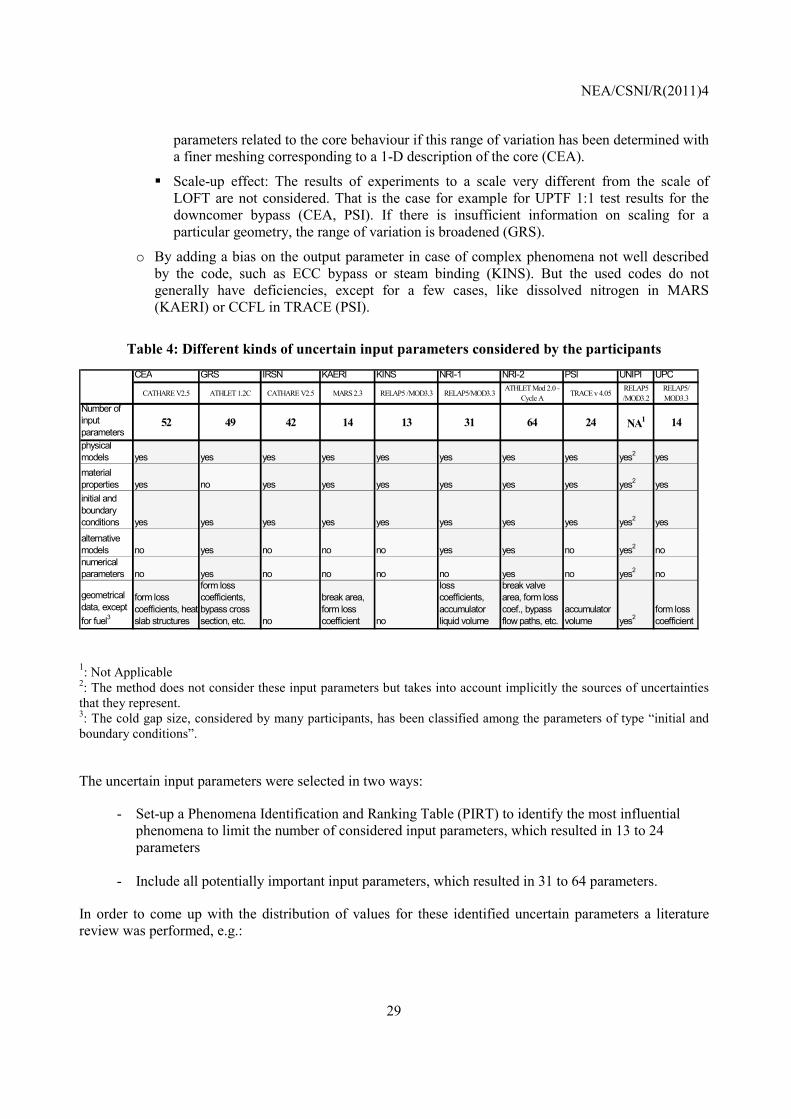
NEA/CSNI/R(2011)4
29
parameters related to the core behaviour if this range of variation has been determined with a finer meshing corresponding to a 1-D description of the core (CEA).
Scale-up effect: The results of experiments to a scale very different from the scale of LOFT are not considered. That is the case for example for UPTF 1:1 test results for the downcomer bypass (CEA, PSI). If there is insufficient information on scaling for a particular geometry, the range of variation is broadened (GRS).
o By adding a bias on the output parameter in case of complex phenomena not well described by the code, such as ECC bypass or steam binding (KINS). But the used codes do not generally have deficiencies, except for a few cases, like dissolved nitrogen in MARS (KAERI) or CCFL in TRACE (PSI).
Table 4: Different kinds of uncertain input parameters considered by the participants
1: Not Applicable 2: The method does not consider these input parameters but takes into account implicitly the sources of uncertainties that they represent. 3: The cold gap size, considered by many participants, has been classified among the parameters of type “initial and boundary conditions”.
The uncertain input parameters were selected in two ways:
- Set-up a Phenomena Identification and Ranking Table (PIRT) to identify the most influential phenomena to limit the number of considered input parameters, which resulted in 13 to 24 parameters
- Include all potentially important input parameters, which resulted in 31 to 64 parameters.
In order to come up with the distribution of values for these identified uncertain parameters a literature review was performed, e.g.:
CEA GRS IRSN KAERI KINS NRI-1 NRI-2 PSI UNIPI UPC
CATHARE V2.5 ATHLET 1.2C CATHARE V2.5 MARS 2.3 RELAP5 /MOD3.3 RELAP5/MOD3.3ATHLET Mod 2.0 -
Cycle A TRACE v 4.05RELAP5 /MOD3.2
RELAP5/ MOD3.3
Number of input parameters
52 49 42 14 13 31 64 24 NA1 14
physical models yes yes yes yes yes yes yes yes yes2 yesmaterial properties yes no yes yes yes yes yes yes yes2 yesinitial and boundary conditions yes yes yes yes yes yes yes yes yes2 yes
alternative models no yes no no no yes yes no yes2 nonumerical parameters no yes no no no no yes no yes2 no
geometrical data, except for fuel3
form loss coefficients, heat slab structures
form loss coefficients, bypass cross section, etc. no
break area, form loss coefficient no
loss coefficients, accumulator liquid volume
break valve area, form loss coef., bypass flow paths, etc.
accumulator volume yes2
form loss coefficient
NEA/CSNI/R(2011)4
30
- Uncertainties about initial and boundary conditions, including the fuel thermal behaviour, was found in the LOFT L2-5 documentation or in the specifications provided by UNIPI for phase II of BEMUSE.
- RELAP5 Code Manuals were used by some users (KINS and NRI-1, but not UPC) and also users of MARS 2.3 (KAERI).
- Depending on the participants, assessment studies were performed (mainly by GRS and PSI).
- Previous analyses were used, either already performed by the participant (GRS, KINS, NRI-1, NRI-2, UPC) or investigations like CSAU [1] (KAERI, PSI) or UMS [12] (GRS, NRI-1, UPC).
Other sources are handbooks for the material properties (KAERI), norms for decay heat power (a majority of participants), sensitivity analyses performed during Phase II of BEMUSE (KAERI), etc.
Another source of information comes from code validation fitting experimental data, mainly from separate effects tests, as recommended by GRS, CEA, IRSN, PSI and to a less extent KINS. Validation experience from integral tests is also used.
Expert judgement was used when no experimental data or specific documentation was available. It was also extensively used due to lack of time for detailed investigations.
4.4 Main results
4.4.1 Results of reference calculations
Figure 3 shows the differences of the best-estimate reference or base calculation of the maximum cladding temperature of the users of CATHARE, of ATHLET and of RELAP5/Mod3.3 or Mod3.2. One finds differences between users applying the same code and partly even the same code version. That user effect has been discussed already in several international comparisons, like International Standard Problems [23]. Data from the experiment are included for comparison.
The most important user’s effect seems to be for both users of CATHARE, but this can be explained. CEA has corrected a mistake in the friction form loss in the accumulator line, found after completion of phase II whereas IRSN did not change the results of Phase II with the aim of performing a blind calculation for phases II and III. Before this correction, both time trends were very close.
The dispersion of the best-estimate calculations is significantly lower than the widths of the uncertainty bands. It should be noted that the comparisons in
Figure 3 show only the user’s effect on the base case calculations. An uncertainty analysis intends to cover effects of an experienced user, but not mistakes of friction form loss.

NEA/CSNI/R(2011)4
31
Maximum cladding temperature: RELAP 5 calculations
200
400
600
800
1000
1200
0 10 20 30 40 50 60 70 80 90 100time (s)
tem
pera
ture
(K)
experimentKINSNRI-1UNIPI (Mod3.2)UPC
Figure 3: Best-estimate reference or base calculation of the maximum cladding temperature for different users of the same code compared with experimental measurements
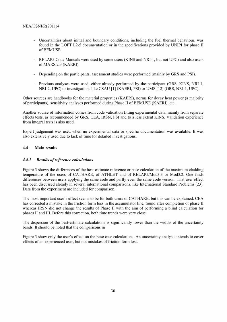
4.4.2 Results of uncertainty analysis
As a requirement for the output, 5% and 95% percentiles had to be determined for six output parameters, which were of two kinds:
• Scalar output parameters
- First Peak Cladding Temperature (PCT)
- Second Peak Cladding Temperature
- Time of accumulator injection
- Time of complete quenching of fuel rods
Maximum cladding temperatures: CATHARE calculations
200
400
600
800
1000
1200
0 10 20 30 40 50 60 70 80 90 100time (s)
tem
pera
ture
(K)
experimentCEAIRSN
Maximum cladding temperature: ATHLET calculations
200
400
600
800
1000
1200
0 10 20 30 40 50 60 70 80 90 100time (s)
tem
pera
ture
(K)
experimentGRSNRI-2
NEA/CSNI/R(2011)4
32
• Time trend output parameters
- Maximum cladding temperature
- Upper plenum pressure
The complete results including the uncertainty bands versus time are presented in the phase III report [15].
1st PCT: uncertainty bounds ranked by increasing band width
600
700
800
900
1000
1100
1200
1300
GRS PSI UPC UNIPI NRI-2 NRI-1 CEA IRSN KAERI KINSorganisation name
tem
pera
ture
(K)
lower uncertainty boundreference upper uncertainty boundexperiment
Figure 4: Uncertainty analysis results for the four single-valued output parameters compared with experimental data
The results of uncertainty bands for the four single-valued output parameters first peak cladding temperature, second peak cladding temperature, time of accumulator injection and time of complete quenching are presented in Figure 4. They are ranked by increasing order of the band width. The following observations can be made:
• First PCT: The spread of the uncertainty bands is within 138-471 K. The difference among the upper 95%/ 95% uncertainty bounds, which is important to compare with the regulatory acceptance criterion, is up to 150 K and all but one participant cover the experimental value. One
2nd PCT: uncertainty bounds ranked by increasing band width
500
600
700
800
900
1000
1100
1200
1300
PSI GRS UPC NRI-1 IRSN UNIPI NRI-2 KINS CEA KAERIorganisation name
tem
pera
ture
(K)
lower uncertainty boundreference upper uncertainty boundexperiment
time of accumulator injection: uncertainty bounds ranked by increasing band width
6
8
10
12
14
16
18
20
22
24
KINS PSI IRSN CEA GRS KAERI NRI-1 UPC NRI-2 UNIPIorganisation name
time
(s)
lower uncertainty boundreference upper uncertainty boundexperiment
time of complete quenching: uncertainty bounds ranked by increasing band width
20
40
60
80
100
120
140
UPC PSI NRI-2 NRI-1 UNIPI GRS KAERI CEA KINS IRSNorganisation name
time
(s)
lower uncertainty boundreference upper uncertainty boundexperiment

NEA/CSNI/R(2011)4
33
participant (UPC) does not envelop the experimental PCT, due to a too high lower bound. Two reasons can explain this result: Among all the participants, on the one hand, UPC has the highest reference value; on the other hand, its band width is among the narrowest ones. KINS attribute their low lower uncertainty bound to a too high value of maximum gap conductance.
• Second PCT: In this case, one participant (PSI) does not envelop the experimental PCT, due to a too low upper bound. The reasons are roughly similar to those given for the first PCT: PSI, as several participants, calculates a too low reference value, but has also the specificity to consider an extremely narrow upper uncertainty band. The spread of the uncertainty bands is within 127-599 K. The difference among the upper 95%/ 95% uncertainty bounds, which is important to compare with the regulatory acceptance criterion, is up to 200 K.
• Time of accumulator injection: Four participants among ten calculate too low upper bounds (KINS, PSI, KAERI and UPC), whereas CEA finds an upper bound just equal to the experimental value. These results are in relationship with the prediction of the cold leg pressure reaching the accumulator pressure 4.29 MPa. The band widths vary within 0.7-5.1 s for all the participants except for UNIPI which finds a much larger band, equal to 15.5 s. This is due to the time error of the pressure transient calculated by UNIPI.
• Time of complete quenching: All the uncertainty bands envelop the experimental value, even if the upper bound is close to the experimental value for one participant. The width of the uncertainty range varies from 10 s to more than 78 s. If the core is not yet quenched at the end of the calculation as it is the case for two participants (KAERI, KINS), or if there are several code failures before the complete quenching (IRSN), the upper bound is plotted at 120 s in Figure 4.
4.4.3 Results of sensitivity or influence analysis
Sensitivity analysis is here a statistical procedure to determine the influence of uncertain input parameters on the uncertainty of the output parameter (result of code calculations). Such a sensitivity analysis is different to the single parameter sensitivity analysis performed within BEMUSE phases II and IV investigating the effect of variations of a single input parameter on a code result.
The only participant not using a fully statistical method (UNIPI) provided some sensitivity studies for the phase II programme (as the majority of participants) but some extra sensitivity studies concerning the gap size value had been added for phase III. The comparison of these sensitivities was provided in the phase II report.
All other participants provide sensitivity or “influence” results from their computations obtained with the randomly generated parameters used during the propagation process to determine the uncertainty of code results discussed before (59 to 150 code runs depending on the participants). They used for example Pearson’s Correlation Coefficients, Standardized Regression Coefficients (SRC), Partial Correlation Coefficients (PCC) which are based on linear dependencies between output and inputs. For monotonic dependency the same coefficients are used, replacing the output and inputs by their ranks.
Each participant provided a table of the most relevant parameters for the four single valued output parameters and for the two time trends (maximum cladding temperature and upper-plenum pressure), based on their influence measures. To synthesize and to compare the results of these influences, there are grouped in two main “macro” responses.

NEA/CSNI/R(2011)4
34
Phenomena and parameters influential for the core cladding temperatures:
• 1st PCT
• 2nd PCT
• Time of the quenching completion
• Maximum cladding temperature as a function of time (before quenching)
Phenomena and parameters influential for the primary pressure behaviour:
• Time of the accumulator injection
• Upper-plenum pressure versus time, mainly before roughly 30 s
For each participant, each parameter is ranked according to its influence on these two kinds of macro-responses. For parameters quoted in their table of relevant parameters, a kind of new ranking (from 0 to 3) of relevance by the “influence” measures is given for both macro-responses:
• 0: the parameter is considered by the participant but never appear as relevant
• 1: for the low relevant parameter
• 2: for medium relevant parameter
• 3: for the highest level of relevance
It must be noted that the total ranking of a parameter cannot exceed 3 for one participant, even if it is found as being relevant for several outputs contributing to a macro-response. For example, a form loss which is very influential both for the time of accumulator injection and for the upper plenum pressure will have a final rank equal to 3 (and not 3 + 3 = 6).
This ranking is quite arbitrary, for example because the difference between a medium and a high level of relevance is not always obvious. Nevertheless, this part of arbitrariness does not change the conclusions and consequently can be considered as acceptable.
For each parameter, the ranking is summed up from all the participants and that result is considered as the total ranking of a parameter. Concerning the influence on the cladding temperature as the “macro-response” combining the 1st and the 2nd PCT, the time of complete quenching and the time trend “maximum cladding temperature”, among the initial amount of more than 150 parameters, 41 have been quoted at least once by one participant as relevant parameters.
The summary of the total ranking by participants for all parameters (whose total ranking is not zero) is shown in Figure 5 for cladding temperature. Such information is useful as a data base for further uncertainty analysis of LB-LOCA.

NEA/CSNI/R(2011)4
35
0 5 10 15
core pressure dropform loss in broken loop HL, in DC/CL at branch
fraction of water and steam in total wall frictioncritical flow subcooledcritical flow two-phase
break areabreak discharge coefficient
initial core powerpeaking factor
gap sizedecay power
UO2 conductivitygap conductivityUO2 specific heat
liquid forced convection HTCnucleate boiling HTC
vapor forced convection HTCfilm boiling HTC
conduction term of the wall to fluid HT in the film boiling regimeheat transfer in the dry zone HTC (global in reflood)
transition film boilingpool film boiling at natural convection
complex of heat transfer modelsminimum film boiling temperature
Critical Heat Flux CHF selection of correlations
dispersed flow interfacial shearinterfacial shear in non-dispersed vertical pipe flow
interfacial shear in non-dispersed vertical bundle flowinterfacial shear in non-dispersed vertical DC flow
interfacial shear in bundle: alternative model CCFL in the upper core plate: c of Wallis correlation
CCFL in the UP: m of Kutateladze correlationinterfacial shear in stratified flow
transition velocity from stratified to slug flow in horizontal pipesnumber of vapor bubbles per unit volume
pressurizer initial levelO-D module: bubble rise velocityHTC of rewetted side, upper QF
initial intact loop cold leg temperature
para
met
ers
total ranking
k = 11< k <7k ≥ 7
accounted by k particpants
Figure 5: Total ranking of the sensitivity or influence of uncertain input parameters on the cladding temperature per parameter
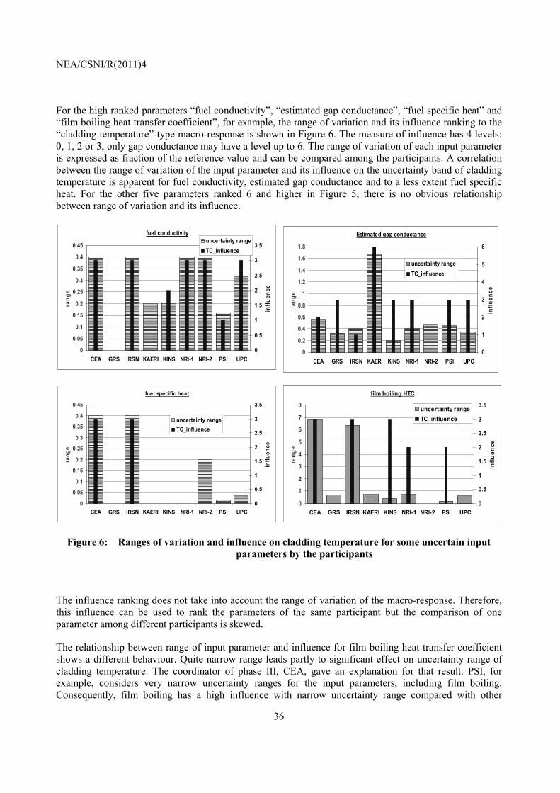
NEA/CSNI/R(2011)4
36
For the high ranked parameters “fuel conductivity”, “estimated gap conductance”, “fuel specific heat” and “film boiling heat transfer coefficient”, for example, the range of variation and its influence ranking to the “cladding temperature”-type macro-response is shown in Figure 6. The measure of influence has 4 levels: 0, 1, 2 or 3, only gap conductance may have a level up to 6. The range of variation of each input parameter is expressed as fraction of the reference value and can be compared among the participants. A correlation between the range of variation of the input parameter and its influence on the uncertainty band of cladding temperature is apparent for fuel conductivity, estimated gap conductance and to a less extent fuel specific heat. For the other five parameters ranked 6 and higher in Figure 5, there is no obvious relationship between range of variation and its influence.
fuel conductivity
0
0.05
0.1
0.15
0.2
0.25
0.3
0.35
0.4
0.45
CEA GRS IRSN KAERI KINS NRI-1 NRI-2 PSI UPC
rang
e
0
0.5
1
1.5
2
2.5
3
3.5
influ
ence
uncertainty rangeTC_influence
fuel specific heat
0
0.05
0.1
0.15
0.2
0.25
0.3
0.35
0.4
0.45
CEA GRS IRSN KAERI KINS NRI-1 NRI-2 PSI UPC
rang
e
0
0.5
1
1.5
2
2.5
3
3.5
influ
ence
uncertainty rangeTC_influence
Figure 6: Ranges of variation and influence on cladding temperature for some uncertain input parameters by the participants
The influence ranking does not take into account the range of variation of the macro-response. Therefore, this influence can be used to rank the parameters of the same participant but the comparison of one parameter among different participants is skewed.
The relationship between range of input parameter and influence for film boiling heat transfer coefficient shows a different behaviour. Quite narrow range leads partly to significant effect on uncertainty range of cladding temperature. The coordinator of phase III, CEA, gave an explanation for that result. PSI, for example, considers very narrow uncertainty ranges for the input parameters, including film boiling. Consequently, film boiling has a high influence with narrow uncertainty range compared with other
Estimated gap conductance
0
0.2
0.4
0.6
0.8
1
1.2
1.4
1.6
1.8
CEA GRS IRSN KAERI KINS NRI-1 NRI-2 PSI UPC
rang
e
0
1
2
3
4
5
6
influ
ence
uncertainty rangeTC_influence
film boiling HTC
0
1
2
3
4
5
6
7
8
CEA GRS IRSN KAERI KINS NRI-1 NRI-2 PSI UPC
rang
e
0
0.5
1
1.5
2
2.5
3
3.5
influ
ence
uncertainty rangeTC_influence

NEA/CSNI/R(2011)4
37
participants. Therefore, a clear relationship between range of variation and its influence can not be expected when all the participants are considered.
4.5 Additional investigations using statistical methods
Some interesting additional investigations were performed in the frame of BEMUSE phase III. These are documented in the phase III report [15] and some of them are selected here.
It is well known that (95%/95%) tolerance limits obtained by order statistics according to Wilks’ formula, overestimate the 95% percentile or quantile conservatively by 95% of the samples. One measure to reduce the “conservatism” and the scatter of results of that tolerance limit is to increase the number of calculations, i.e. increase the order of Wilks’ formula, Figure 7. This is a statistical convergence theorem. Another way is to assume a distribution of the output variable, e.g. normal distribution and to check such a distribution by a suitable statistical test [16]. In these cases one obtains less conservative bounds with the same number of calculations, or the same “conservatism” with a lower number of calculations. This procedure was not applied in phase III but by one participant in phase V of the BEMUSE programme, and is mentioned here for completeness.
Figure 7: Statistical convergence of a 95%/95% tolerance limit, or decreasing “conservatism” with
increasing number of calculation runs, shown as probability distributions
PDF of Wilks’s 0.95%/95%-limits for various sample sizes
percentile1.0 0.980.960.940.92
60.0
40.0
20.0
0.0
59
93124153
234
311
555
0.95

NEA/CSNI/R(2011)4
38
4.5.1 Investigation of statistical convergence of tolerance limits by increasing the number of code runs
Five participants have increased the number of code runs with respect to their base case, as shown in Table 5.
Table 5: Number of code runs and investigated output parameters
CEA IRSN KAERI NRI-1 NRI-2 Base case: number of code runs
100 59 100 59 60
Increased number of code runs
1003 590 3500 93 100 / 1000
Considered output parameters
1st PCT 1st PCT 1st and 2nd PCT Temperature-type outputs + time of accumulator injection
Temperature-type outputs + time of accumulator injection
Upper tolerance limits obtained in the base case
1st PCT: 1246 K 1st PCT: 1233 K 1st PCT: 1218 K 2nd PCT: 1197 K
1st PCT: 1208 K 2nd PCT: 1167 K
1st PCT: 1165 K 2nd PCT: 1185 K
NRI-1 has performed 34 additional code runs to compare the results of uncertainty analysis obtained by using Wilks’ formula at the second order with respect to those obtained at the first order. The difference of results is only minor. Other participants have significantly increased their number of code runs, some of them comparing only the first PCT to avoid problems of code failures in the later transient. The information gained from these calculations is related to both uncertainty analysis and sensitivity analysis, described in the following sections.
4.5.1.1 Uncertainty Analysis
The most important conclusions are: The dispersion of the upper tolerance limit obtained by using Wilks’ formula at the first and the second order was investigated by CEA and KAERI. Both organizations have divided their N code results into several separate samples of size n = 59 and for each sample, have considered the highest value of the output (Wilks at the first order). For CEA, the spread of this tolerance limit is about 150 K for the 1st PCT, whereas KAERI finds roughly 200 K for the 1st PCT and 250 K for the 2nd PCT. KAERI has also performed the same work with samples of 93 code results and by applying Wilks’ formula at the second order. The dispersion of second order results is half of first order. An estimate to determine directly the empirical 95% percentile is possible with a high number of calculations. CEA and KAERI show that this estimate converges from 600 to 700 code runs for the blowdown PCT, and for 1000 code runs for the reflood PCT. The obtained values are lower than the upper tolerance limits obtained by using Wilks’ formula at the first or the second order, which is obvious since

NEA/CSNI/R(2011)4
39
the upper tolerance limits are higher than the 95% percentile in 95% of the cases (β = 95%): For example, the difference is 30 K for the CEA calculations.
IRSN evaluated the 95% uncertainty band of the estimated 95% percentile. Its width is estimated either from the properties of the Beta law or by Bootstrap (resampling by using the original parameter selections) [17]. Both methods give finally comparable results, the width of the 95% uncertainty band decreases with the number of code runs, converging at roughly 300 to 400 code runs.
Other investigated issues are:
The determination of the upper tolerance limit of the same percentile (α = 95%) with the same confidence level (β = 95%) as in the base case, but by applying Wilks’ formula at a higher order since the number of code runs is higher. In this way, CEA finds 1225 K for the 1st PCT (Wilks at the order 39 = minimum 991 runs, performed were 1003 runs) to be compared to 1246 K in its base case (Wilks at the second order, 100 runs), whereas IRSN finds 1186 K (590 runs) to be compared to 1233 K in its base case (Wilks at the first order, 59 runs). Increasing the number of code runs (samples) converges the percentile towards the theoretical one (α = 95%).
A further possibility is to increase the confidence level β, i.e. the probability to exceed the percentile. Considering an upper limit of the same percentile α = 95%, but with a higher β confidence level, CEA and IRSN find 1239 K and 1198 K with β = 99.99% instead of 1225 K and 1186 K with β = 95%. NRI-2 considers Wilks at the first order and consequently increases β when increasing the number of code runs. For example, they find for the 1st PCT 1165 K with 60 code runs and β = 95%, 1201 K with 100 code runs and β = 99.4%, 1211 K with 1000 code runs and β almost equal to 1.
The already mentioned, USNRC Regulatory Guide 1.157 [7] as well as the IAEA SSG-2 [11] requires that the applicable acceptance criteria will not be exceeded with a probability of 95% or more. If additional confidence levels are used, at least 95% confidence levels should be applied. Therefore, 95%/ 95% statements are recommended for licensing applications. As seen above, a higher confidence level results in higher upper limits of the cladding temperature, for example. An upper limit close to the theoretical 95% percentile, mentioned at begin of section 4.5, is not required for licensing applications because the percentile may be higher than 95%. However, a 95%/ 95% statement can be satisfied with higher convergence (lower conservatism) and a lower dispersion if the number of code runs is increased.
4.5.1.2 Sensitivity Analysis
All those participants applying the statistical method use influence measures based on ranks (Spearman’s Correlation Coefficient or Spearman’s Rank Regression Coefficient). Some organisations observed a change of influence measures with increasing number of code runs. Those parameters showing the highest sensitivity measures, however, do not change their influence. This is a proof that the most influential variables have a monotonous effect on the code responses. The influence is changed for those parameters which are not statistically relevant.
One explanation for the change of ranking when the number of code runs is increased may be the existence of spurious correlations between the input parameters if the number of code runs is low compared with the number of input parameters (CEA, IRSN, NRI-2). Spurious correlations are artificial correlations between parameters. Spurious correlations disappear if the number of code runs is increased. They can also be detected by comparing the results of different sensitivity measures. It must be noted that this discussion on number of calculations with regard to ranking is relevant for sensitivity analysis but not for the uncertainty

NEA/CSNI/R(2011)4
40
analysis applying Wilks’ formula. The number of calculations should be higher than that of uncertain input parameters when also lower influences are to be determined.
4.5.2 Modifying the type of probability distribution and truncation
CEA, which uses only normal and log-normal distributions for uncertain input parmeters truncated at µ ± 3.09σ in its base case, has carried out two tests. They performed 100 calculations each, using the same selection of parameter values for both ranges.
400
500
600
700
800
900
1000
1100
1200
1300
0 10 20 30 40 50
time (s)
tem
pera
ture
(K)
reference caseuniform sampling (case 1)truncation at ±2*sigma (case 2)experiment
Figure 8: Comparison of upper bound of calculated cladding temperature due to changes of
distribution of input uncertainties In the first test, all the normal and log-normal density functions of the inputs are replaced by uniform and log-uniform ones, and truncations of µ ± 2σ and e(µ ± 2σ), respectively. The influence of this change of distribution on the upper bound of the maximum cladding temperature is investigated. The upper bound of the cladding temperature increased by 30 K for the 1st PCT, see Figure 8.
In the second test, the normal and log-normal laws are kept but truncated at µ ± 2σ instead of µ ± 3.09σ (reference or base case). This time, it leads to a slight decrease of the upper bound of the maximum cladding temperature by 15 K for the 1st PCT, Figure 8.
For comparison the measured cladding temperature is presented in Figure 8 which is bounded by the calculated upper tolerance limits up to 30 seconds.

NEA/CSNI/R(2011)4
41
4.6 Conclusions of phase III
The main lessons learned from phase III are:
For uncertainty and sensitivity analysis, all the participants used a statistical method according to the use of Wilks’ formula, except UNIPI applied its CIAU method. Use of both methods was successfully mastered.
Compared with the experiment, the results of uncertainty analysis are good on the whole. For example, for the cladding temperature-type output parameters (1st PCT, 2nd PCT, maximum cladding temperature versus time, time of complete quenching), 8 participants out of 10 find upper and lower bounds which envelop the experimental data.
Differences can be seen in the results of different participants with regard to the base case or reference calculations, the maximum differences between two participants are 151 K for the 1st PCT (UPC-PSI) and 213 K for the 2nd PCT (UPC-UNIPI). These differences among participants are lower compared to the results in Phase II. Some reference calculations were changed compared to Phase II. The maximum difference among the participants’ upper 95%/ 95% uncertainty limits, which are important to compare with the regulatory acceptance criterion, is for both PCTs in the same range as for the reference calculations of Phase III: 158 K for the 1st PCT (CEA-KINS), 208 K for the 2nd PCT (UPC-PSI). Differences between the calculated uncertainty upper limits and their distance to the base case calculations are from 28 K (GRS, 2nd PCT) to 207 K (NRI2, 2nd PCT). They may be due to the different ranges of input uncertainties between the participants.
Nevertheless, the same ranges can lead to very different results, as shown in Figure 2 of the part devoted to Phase II. But for this figure, the considered ranges were partly unrealistically, what is not the case for Phase III. Results from Phase IV with realistic ranges show less differences between participants.
The number of the uncertain input parameters is not important; NRI2 considered 64 and GRS 49, the others in between the calculated range identified 52, 42, 31, 24, 14, and 13. However, all influential parameters should be included, otherwise the uncertainty band for the outputs may be too narrow.
Comparisons of results of the upper 95%/95% bound of PCT applying Wilks’ formula at higher order with an increased number of code runs resulted in differences which are low compared with the highest differences between participants of 150 K to 200 K above. These examples show clearly the higher importance of results of the base calculation and selected input uncertainties and their ranges on the uncertainty bounds compared to the number of calculations.
Sensitivity analysis has been successfully performed by all participants using the statistical method. The used importance measures take into account the range of variation of the input parameters. Synthesis tables of the most influential phenomena and parameters were prepared and participants could use these for the next step of the BEMUSE programme. It seems sufficient and satisfactory to identify the dominating uncertain input parameters, i.e. those few with the highest influence on the output uncertainty. These can be identified if a sufficient number of code runs is performed, i.e. for sensitivity measures more calculations than input uncertainties should be performed.
A change of the distribution of input uncertainties within approximately the same range has a relative low influence on the upper tolerance limit of cladding temperature compared with the differences of base case calculation results and the variation of input uncertainty ranges.

NEA/CSNI/R(2011)4
42
First suggestions for improvement of the methods have not been proposed as result of the exercise; however, recommendations for proper application of the statistical method were given, see Section 7.7. In order to reduce the dispersion of uncertainty results, it was proposed to set-up a common list of uncertain input parameters for initial and boundary conditions with their distributions and ranges for the phase V exercise.

NEA/CSNI/R(2011)4
43
5. BEMUSE PHASE IV
The scope of phase IV is the simulation of a LBLOCA in a Nuclear Power Plant using experience gained in phase II. Calculation results were the basis for uncertainty evaluation, to be performed in the next phase. The objectives of the activity are [18]:
− To simulate a LBLOCA reproducing the phenomena associated to the scenario. − To have a common, well-known basis for the future comparison of uncertainty evaluation
results among different methodologies and codes. The activity for the Zion Nuclear Power Plant was similar to the previous phase II for the LOFT experiment. The UPC team together with UNIPI provided the database for the plant, including RELAP5 and TRACE input decks. Geometrical data, material properties, pump information, steady state values, initial and boundary conditions, as well as sequence of events were provided. The nodalisation comprised generally more hydraulic nodes and axial nodes in the core compared with the LOFT applications. Participants were the same as for phase V, except NRI-2 (J. Macek) that did not participate in phase IV. The highest difference in calculated maximum peak cladding temperatures (PCT) between the participants is 167 K (EDO: 1326, KAERI: 1159 K), what is lower than the difference of BEMUSE phase II calculations of the LOFT test. The calculated maximum cladding temperatures are shown in Figure 9. Experimental data were available for phase II to compare with, but not for phase IV. A list of sensitivity calculations was proposed by UPC and performed by the participants to study the influence of different parameters, such as material properties, initial and boundary conditions upon the influence of relevant output parameters in the scenario under investigation, i.e. a LB LOCA of a cold leg, Table 6. The ranges of variations are realistic compared with those of phase II. The last two parameter ranges in Table 6 refer to tables in [18]. Parameter no. 3, power after scram, is based on “Decay Heat Power in LWR”, ANSI/ANS-5.1, 1979; Table A.48 in [18]. The variation of containment pressure (sensitivity no. 9) was up to 0.1 MPa lower than the reference case versus time. The sensitivity of hot/ cold conditions for pellet radius (sensitivity no. 10) was intended to decrase or increase the average pellet temperature by ±75 K for the node having the maximum linear power. It is said that this is equivalent to gap width zero at cold conditions, i.e. the pellet is in contact with the cladding. The results were less different between participants than found in phase II. The maximum difference of calculated maximum ∆PCT of participants was 103 K for the lower range of maximum linear power (UPC: -5.4 K, GRS: -108.0 K), Figure 10. The nodalisation of the core was similar; both organisations used two core channels and 18 axial nodes per channel. A reason for the difference of results from participants using the same values for input parameter variations may be different models for the same heat transfer regime in different codes, different changes of heat transfer regimes during the transient due to different nodalisations and due to other selections in the input decks.

NEA/CSNI/R(2011)4
44
Figure 9: Calculated maximum cladding temperature versus time
Table 6: Parameters to vary for sensitivity analysis

NEA/CSNI/R(2011)4
45
Figure 10: Effect of variation of maximum linear power (sensitivity no. 5) on PCT and ∆tReflood
Figure 11: Effect of parameter variation on average change of PCT values
∆PCT = 60 K
∆PCT = 103 K

NEA/CSNI/R(2011)4
46
Figure 10 contains values for ∆PCT as well as calculated difference in reflood time ∆tReflood, what is meant as difference in total quench time, for the minimum and maximum values of the input parameter range in Table 6.
Figure 11 represents the averaged ∆PCT values when the sensitive input parameter changes from its lower to its upper value. In addition, the standard deviation of the PCT ranges of the participants is included. Most influential input parameters on PCT are those related to energy stored in the fuel. The influential input parameters are fuel and gap conductivity, power before and after scram and fuel dimensions. That is consistent with findings from phase II and III, as well as phase V, described in the next Chapter.
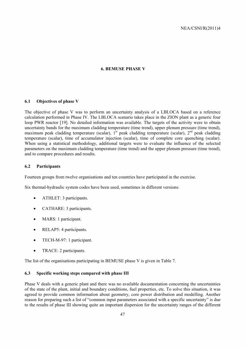
NEA/CSNI/R(2011)4
47
6. BEMUSE PHASE V
6.1 Objectives of phase V
The objective of phase V was to perform an uncertainty analysis of a LBLOCA based on a reference calculation performed in Phase IV. The LBLOCA scenario takes place in the ZION plant as a generic four loop PWR reactor [19]. No detailed information was available. The targets of the activity were to obtain uncertainty bands for the maximum cladding temperature (time trend), upper plenum pressure (time trend), maximum peak cladding temperature (scalar), 1st peak cladding temperature (scalar), 2nd peak cladding temperature (scalar), time of accumulator injection (scalar), time of complete core quenching (scalar). When using a statistical methodology, additional targets were to evaluate the influence of the selected parameters on the maximum cladding temperature (time trend) and the upper plenum pressure (time trend), and to compare procedures and results.
6.2 Participants
Fourteen groups from twelve organisations and ten countries have participated in the exercise.
Six thermal-hydraulic system codes have been used, sometimes in different versions:
• ATHLET: 3 participants.
• CATHARE: 3 participants.
• MARS: 1 participant.
• RELAP5: 4 participants.
• TECH-M-97: 1 participant.
• TRACE: 2 participants.
The list of the organisations participating in BEMUSE phase V is given in Table 7.
6.3 Specific working steps compared with phase III
Phase V deals with a generic plant and there was no available documentation concerning the uncertainties of the state of the plant, initial and boundary conditions, fuel properties, etc. To solve this situation, it was agreed to provide common information about geometry, core power distribution and modelling. Another reason for preparing such a list of “common input parameters associated with a specific uncertainty” is due to the results of phase III showing quite an important dispersion for the uncertainty ranges of the different

NEA/CSNI/R(2011)4
48
participants. A list of common uncertain input parameters concerning uncertainties of the nuclear power plant was prepared by CEA, GRS and UPC teams. These parameters were strongly recommended to be used in the uncertainty analysis when a statistical approach was followed. The list specified the parameter, the distribution type and their range; it is shown in Table 8.
Table 7: List of participants in BEMUSE Phase V
Numb. Organisation Country Name Code 1 AEKI Hungary A. Guba
I. Tóth I. Trosztel
ATHLET 2.0A
2 CEA France T. Mieusset P. Bazin A. de Crécy
CATHARE2 V2.5_1 (r5_567)
3 EDO “GIDROPRESS”
Russia S. Borisov TECH-M-97
4 GRS Germany T. Skorek H. Glaeser
ATHLET 2.1B
5 IRSN France J. Joucla P. Probst
CATHARE2 V2.5_1 mod6.1
6 JNES Japan A. Ui TRACE ver4.05 7 KAERI South Korea B.D .Chung MARS 3.1 8 KINS South Korea D.Y. Oh RELAP5/mod3.3 9 NRI-1 Czech Republic R. Pernica
M. Kyncl RELAP5/mod3.3
10 NRI-2 Czech Republic J. Macek ATHLET 2.1 A 11 PSI Switzerland A. Manera
J. Freixa TRACE5rc3
12 UNIPI-1 Italy A. Petruzzi F. D’Auria
RELAP5/mod3.2
13 UNIPI-2 Italy A. Del Nevo F. D’Auria
CATHARE2 V2.5_1 mod6.1
14 UPC Spain M. Pérez F. Reventós L. Batet
RELAP5/mod3.3
Table 8: Common input parameters associated with a specific uncertainty, range of variation and type of probability density function.
Phenomenon Parameter Imposed range of variation
Type of pdf
Comments
Flow rate at the break
Containment pressure
[0.85, 1.15] Uniform Multiplier.
Fuel thermal behaviour
Initial core power
[0.98; 1.02] Normal Multiplier affecting both nominal power and the power after scram.
Peaking factor (power of the hot rod)
[0.95; 1.05] Normal Multiplier.
Hot gap size (whole core except hot rod)
[0.8; 1.2]
Normal Multiplier. Includes uncertainty on gap and cladding conductivities.

NEA/CSNI/R(2011)4
49
Phenomenon Parameter Imposed range of variation
Type of pdf
Comments
Hot gap size (hot rod)
[0.8; 1.2]
Normal Multiplier. Includes uncertainty on gap and cladding conductivities.
Power after scram
[0.92; 1.08] Normal Multiplier
UO2 conductivity
[0.9, 1.1] (Tfuel <2000 K ) [0.8,1.2] (Tfuel >2000 K)
Normal Multiplier. Uncertainty depends on temperature.
UO2 specific heat
[0.98, 1.02] (Tfuel <1800 K ) [0.87,1.13] (Tfuel >1800 K)
Normal Multiplier. Uncertainty depends on temperature.
Pump behaviour
Rotation speed after break for intact loops
[0.98; 1..02] Normal Multiplier.
Rotation speed after break for broken loop
[0.9; 1.1] Normal Multiplier.
Data related to injections
Initial accumulator pressure
[-0.2; +0.2] MPa Normal
Friction form loss in the accumulator line
[0.5; 2] Log-normal Multiplier.
Accumulators initial liquid temperature
[-10; +10] °C Normal
Flow characteristic of LPIS
[0.95 ; 1.05] Normal Multiplier.
Pressurizer Initial level [-10; +10] cm Normal Initial pressure [-0.1; +0.1] MPa Normal Friction form loss in the surge line
[0.5; 2] Log-normal Multiplier.
Initial conditions: primary system
Initial intact loop mass flow rate
[0.96; 1.04] Normal Multiplier. This parameter can be changed through the pump speed or through pressure losses in the system...
Initial intact loop cold leg temperature
[-2; +2] K Normal This parameter can be changed through the secondary pressure, heat transfer coefficient or area in the U-tubes...
Initial upper-head mean temperature
[Tcold ; Tcold + 10 K]
Uniform This parameter refers to the “mean temperature” of the volumes of the upper plenum (see Annex 1 in Appendix A)
Table 8 gives types of distribution functions and ranges for following parameters:
- Material properties
- Initial and boundary conditions

NEA/CSNI/R(2011)4
50
- Friction form loss factors.
Three participants considered only, and when possible, the set of parameters suggested in the specifications document:
- EDO did not include the following parameters: initial upper head temperature, initial accumulator liquid temperature and hot gap size (zones 1, 2, 3, 4)
- JNES used only the 20 common parameters
- PSI did not consider the upper-head mean temperature parameter of the common parameters due to the use of a 3D vessel nodalization, but considered CCFL at the upper tie plate with the uncertainty distribution in the specifications document.
Participants using a 3D vessel nodalization (CEA, JNES, KAERI and PSI) could not implement directly the “upper-head mean temperature” uncertainty. AEKI, CEA, GRS, IRSN, KINS and PSI groups have used a different reference case calculation in phase V than the one submitted in phase IV.
Table 9 compares the number of uncertain input parameters used by the participants in phases III and V. The differences in considered uncertainties by the participants decreased.
Table 9: Number of input parameters, comparison of phases 3 and 5
AEK
I
CEA
EDO
GR
S
IRSN
JNES
KA
ERI
KIN
S
NR
I1
NR
I2
PSI
UPC
Mea
n
Stan
dard
de
viat
ion
Phase III - 53 - 49 42 27 14 13 31 64 24 14 33.1 18.1 Phase V 36 44 17 55 54 20 25 24 33 44 20 32 33.7 13.2 Phase V (*) 36 44 - 55 54 - 25 24 33 44 - 32 38.6 11.4 (*) Only participants considering more parameters than the proposed common parameters.
Table 10: Order of Wilks' application, comparison of phases 3 and 5
AEK
I
CEA
EDO
GR
S
IRSN
JNES
KA
ERI
KIN
S
NR
I1
NR
I2
PSI
UPC
Phase III -
2 (100) -
2 (100)
1 (59) 1 (100)
2 (100)
1 (59) 1 (59) 1 (60) 3 (150)
2 (100)
Phase V 3 (130)
5 (200)
2 (93) 4 (153)
9 (300)
2 (110)
3 (200)
3 (124)
5 (200)
2 (93) 2 (120)
3 (124)
The comparison of Wilks’ order used in both phases is shown in Table 10 where the number in parenthesis indicates the number of code calculations performed, including failed code runs. No recommendation was made on this number in the specifications document.

NEA/CSNI/R(2011)4
51
Some remarks to Table 10:
- The minimum order for Wilks’s method in phase V is two, while in phase III it was one.
- The general tendency among the participants has been to increase at least one order with respect to phase III. This was recommended at the end of phase III.
- Only one participant (PSI) decreased the number of code runs and the order of Wilks’ formula.
- 4 participants used 2nd order (EDO, JNES, NRI2 and PSI).
- 4 participants used 3rd order (AEKI, KAERI, KINS and UPC).
- 4 participants used higher orders than three (GRS used 4th order, CEA and NRI1 used 5th order, and IRSN used 9th order).
Two participants performed additional analyses by increasing the number of runs and, thus, the order of Wilks’ formula. GRS compared the differences of calculated upper 95%/95% bound of the two peak cladding temperatures between 1st order (59 calculations) and 4th order (153 calculations) with the ATHLET code to be 40 K and 78 K for the 1st PCT and 2nd PCT, respectively [20]. EDO “Gidropress” performed 93 and up to 999 code runs, changing the order of Wilks’ formula from 2 up to 39. The maximum peak cladding temperature was reduced with the higher number of runs by about 35 K, i.e. from 1450 to 1416 K.
1 – Peak cladding temperature determined by Wilks’ formula 2 – normal distribution for 999 code runs
Figure 12: Dispersion of upper tolerance limit of maximum peak cladding temperature dependent on number of code runs performed by EDO “Gidropress”
0 1 0 20 30 40Order of Wi l k
s' formula
1 3 50
1 4 00
1 4 50
1 5 00
T max
__ __ __ _ __ __ K
12
1200 C - accep ta nce criteriono

NEA/CSNI/R(2011)4
52
Results of 999 calculations obtained by EDO “Gidropress” were divided into several separate samples of size n = 59, 93, 124, 153 etc. (which corresponds to Wilk’s formula from 1 up to 39), Figure 12. One can note, that the uncertainty results are less dispersed with increasing sample size, from 95 K to 10 K increasing the code runs from 59 (Wilks’ formula of first order) to 311 (Wilks’ formula of tenth order). It is also important to note that using Wilks’ formula at the low order (first or second order) can predict results close to the acceptance criterion 1477 K or even exceed this criterion in Figure 12, when the reference calculation and the distribution of the results is already relative high compared with other participants, like the EDO results in Figures 20 and 25.
Results of 93 EDO calculations have also been processed assuming that the law of distribution of the calculated values of maximum peak cladding temperature is normal. Mean value is 1323 K and standard deviation is 52.8 K. The maximum peak cladding temperature will be 1410 K for the probability level not less than 95 %. In order to test if the tolerance limit results converge to that value for a high number of calculations, 999 calculations were performed. A comparison of maximum PCT obtained by Wilk’s formula of 2nd and 39th orders and normal law distribution is presented in the next table.
PCT
93 code runs 999 code runs
Wilk’s 2nd order Normal law distribution Wilk’s 39th order Normal law
distribution
UUB (K) 1450 1410 1416 1405
One can note, by assuming normal distribution for the output values, the value of maximum peak cladding temperature decreases slightly by 5 K with increasing number of code runs. A more significant decrease of the upper tolerance limit by 34 K could be observed with 999 code runs according to Wilks’ formula. Still, the difference is relatively small. A distribution of the output variable, e.g. normal or another adequate one can be assumed and checked by a fit test. That allows a direct estimation of the 95th percentile, and allows a significant reduction of code runs. EDO finds that this estimate is almost the same with 93 and 999 code runs. This observation should be confirmed by additional investigations.
6.4 Treatment of failed code runs
For a proper use of the Wilks’ formula all code runs should be terminated successfully or corrected in case of any failure, as already recommended at the end of Phase III. The reason of this is that Wilks’formula is based on a random sample. Leaving out failed code runs leads to the situation, that such a set is not randomly selected any more. However, a relatively low number of failures can be treated in a conservative way by assuming that the n failed runs produced the n most adverse values of the output parameter of interest (e.g. PCT). If the number of overall calculations is high enough to use Wilks 95%/95% formula at the order 2, for example, then the 1 most adverse result can be discarded for a one-sided tolerance limit. For example, for a second order application, requiring α = β = 95%, at least 92 successful code runs (93-1) are needed in case of one failure. The failure is discarded and the maximum value among the successful runs is taken as the 95%/95% estimation.
As an example, let us consider the case of PSI performing 120 code runs with 4 code failures. As explained above, it is not correct to consider that the 116 successful code runs are sufficient to apply Wilks at the order of 2, based on the argument that at this order and for α = β = 95%, only 93 code runs are needed. The 4 failed code runs might correspond with the highest values of the key output variable, if they had been
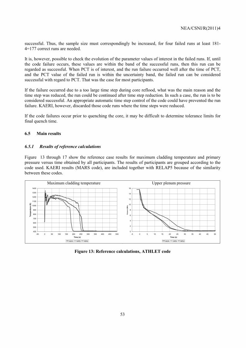
NEA/CSNI/R(2011)4
53
successful. Thus, the sample size must correspondingly be increased, for four failed runs at least 181-4=177 correct runs are needed.
It is, however, possible to check the evolution of the parameter values of interest in the failed runs. If, until the code failure occurs, these values are within the band of the successful runs, then this run can be regarded as successful. When PCT is of interest, and the run failure occurred well after the time of PCT, and the PCT value of the failed run is within the uncertainty band, the failed run can be considered successful with regard to PCT. That was the case for most participants.
If the failure occurred due to a too large time step during core reflood, what was the main reason and the time step was reduced, the run could be continued after time step reduction. In such a case, the run is to be considered successful. An appropriate automatic time step control of the code could have prevented the run failure. KAERI, however, discarded those code runs where the time steps were reduced.
If the code failures occur prior to quenching the core, it may be difficult to determine tolerance limits for final quench time.
6.5 Main results
6.5.1 Results of reference calculations
Figure 13 through 17 show the reference case results for maximum cladding temperature and primary pressure versus time obtained by all participants. The results of participants are grouped according to the code used. KAERI results (MARS code), are included together with RELAP5 because of the similarity between these codes.
Maximum cladding temperature
400
500
600
700
800
900
1000
1100
1200
1300
1400
-50 0 50 100 150 200 250 300 350 400 450 500
Time (s)
Tem
pera
ture
(K)
AEKI GRS NRI2
Upper plenum pressure
0
2
4
6
8
10
12
14
16
-5 0 5 10 15 20 25 30 35 40 45 50
Time (s)
Pres
sure
(MPa
)
AEKI GRS NRI2
Figure 13: Reference calculations, ATHLET code
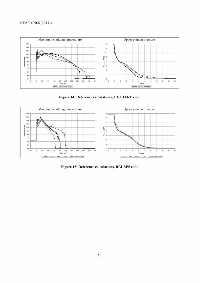
NEA/CSNI/R(2011)4
54
Maximum cladding temperature
400
500
600
700
800
900
1000
1100
1200
1300
1400
-50 0 50 100 150 200 250 300 350 400 450 500
Time (s)
Tem
pera
ture
(K)
CEA IRSN UNIPI2
Upper plenum pressure
0
2
4
6
8
10
12
14
16
-5 0 5 10 15 20 25 30 35 40 45 50
Time (s)
Pres
sure
(MPa
)
CEA IRSN UNIPI2
Figure 14: Reference calculations, CATHARE code
Maximum cladding temperature
400
500
600
700
800
900
1000
1100
1200
1300
1400
-50 0 50 100 150 200 250 300 350 400 450 500
Time (s)
Tem
pera
ture
(K)
KINS NRI1 UNIPI1 UPC KAERI (MARS code)
Upper plenum pressure
0
2
4
6
8
10
12
14
16
-5 0 5 10 15 20 25 30 35 40 45 50
Time (s)
Pres
sure
(MPa
)
KINS NRI1 UNIPI1 UPC KAERI (MARS code)
Figure 15: Reference calculations, RELAP5 code

NEA/CSNI/R(2011)4
55
Maximum cladding temperature
400
500
600
700
800
900
1000
1100
1200
1300
1400
-50 0 50 100 150 200 250 300 350 400 450 500
Time (s)
Tem
pera
ture
(K)
JNES PSI
Upper plenum pressure
0
2
4
6
8
10
12
14
16
-5 0 5 10 15 20 25 30 35 40 45 50
Time (s)
Pres
sure
(MPa
)
JNES PSI
Figure 16: Reference calculations, TRACE code
Maximum cladding temperature
400
500
600
700
800
900
1000
1100
1200
1300
1400
-50 0 50 100 150 200 250 300 350 400 450 500
Time (s)
Tem
pera
ture
(K)
EDO
Upper plenum pressure
0
2
4
6
8
10
12
14
16
-5 0 5 10 15 20 25 30 35 40 45 50
Time (s)
Pres
sure
(MPa
)
EDO
Figure 17: Reference calculation. TECH-M-97 code
6.5.2 Results of uncertainty analysis
6.5.2.1 Single valued results
Again two types of methodologies were applied in the BEMUSE Phase V exercise to obtain the uncertainty bands: “Propagation of input uncertainty” type, used by twelve participants out of the total of fourteen, and “propagation of output accuracy” type, used by one participant, i.e. University of Pisa with two submissions using two different computer codes, RELAP5 and CATHARE. In this case the CIAU was used with two different error databases developed for the RELAP5 and CATHARE codes.
The results can be summarized as follows:
• All participants managed to obtain the requested uncertainty bands with reasonable values.
• A database, including comparative tables and plots has been produced.
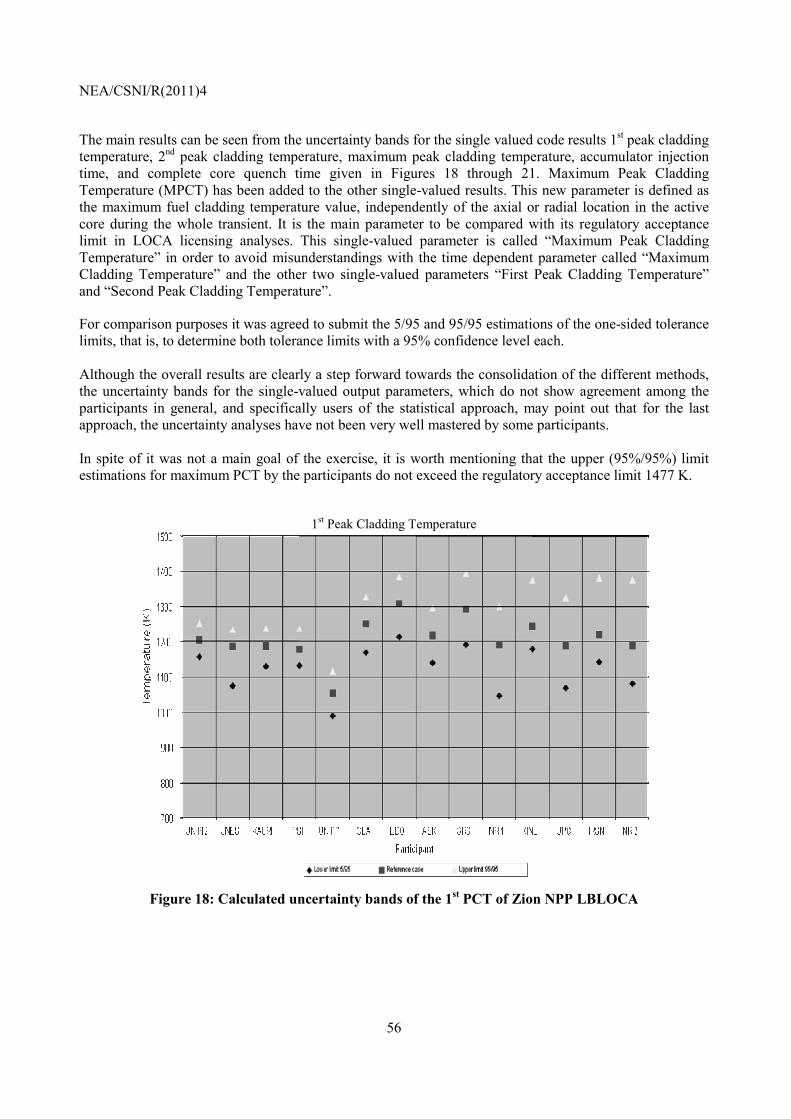
NEA/CSNI/R(2011)4
56
The main results can be seen from the uncertainty bands for the single valued code results 1st peak cladding temperature, 2nd peak cladding temperature, maximum peak cladding temperature, accumulator injection time, and complete core quench time given in Figures 18 through 21. Maximum Peak Cladding Temperature (MPCT) has been added to the other single-valued results. This new parameter is defined as the maximum fuel cladding temperature value, independently of the axial or radial location in the active core during the whole transient. It is the main parameter to be compared with its regulatory acceptance limit in LOCA licensing analyses. This single-valued parameter is called “Maximum Peak Cladding Temperature” in order to avoid misunderstandings with the time dependent parameter called “Maximum Cladding Temperature” and the other two single-valued parameters “First Peak Cladding Temperature” and “Second Peak Cladding Temperature”.
For comparison purposes it was agreed to submit the 5/95 and 95/95 estimations of the one-sided tolerance limits, that is, to determine both tolerance limits with a 95% confidence level each. Although the overall results are clearly a step forward towards the consolidation of the different methods, the uncertainty bands for the single-valued output parameters, which do not show agreement among the participants in general, and specifically users of the statistical approach, may point out that for the last approach, the uncertainty analyses have not been very well mastered by some participants. In spite of it was not a main goal of the exercise, it is worth mentioning that the upper (95%/95%) limit estimations for maximum PCT by the participants do not exceed the regulatory acceptance limit 1477 K.
1st Peak Cladding Temperature
Figure 18: Calculated uncertainty bands of the 1st PCT of Zion NPP LBLOCA

NEA/CSNI/R(2011)4
57
2nd Peak Cladding Temperature
Figure 19: Calculated uncertainty bands of the 2nd PCT of Zion NPP LBLOCA
Maximum peak cladding temperature
Figure 20: Calculated uncertainty bands of the maximum PCT of Zion NPP LBLOCA
700
800
900
1000
1100
1200
1300
1400
1500
JNES NRI1 KAERI PSI GRS EDO UNIPI2 CEA KINS UPC IRSN UNIPI1 AEKI NRI2 Participant
Tem
pera
ture
(K)
Lower limit 5/95 Reference case Upper limit 95/95

NEA/CSNI/R(2011)4
58
Figure 21: Calculated uncertainty bands of the accumulator injection time and complete quenching
of the core of Zion NPP LBLOCA
The following observations can be made:
- One participant (KAERI with MARS code) does not obtain complete core quenching in the upper bound case of the uncertainty band. The reason given is the low range of CHF.
- Two participants (EDO with TECH-M-97 code, NRI2 with ATHLET code) find an upper bound for the maximum peak temperature close to 1477 K – the acceptance criterion for the fuel cladding (difference less than 30 K).
- Participants using CIAU methodology (UNIPI1 with RELAP5 code, UNIPI2 with CATHARE code) obtain a band width for accumulator injection start time larger than the other participants, which is consequence of the primary pressure “uncertainty width” obtained by the CIAU users.
The two approaches to quantify uncertainties, the statistical and UNIPI CIAU methods, give very different results for the uncertainty bands of the primary pressure. This is due to the fact that CIAU approximates the time error on the basis of comparing experimental data and calculations. The various experiments have different time constants.
When comparing results for the maximum PCT, there is an overlap region of, roughly, 15K (between 1221K and 1238K). This region is very small. For the 1st and 2nd PCT the uncertainty bands of all participants show no overlap. When not including participants with extreme values of the uncertainty bands, it is possible to obtain overlap regions for the other two peak cladding quantities. In this case, for the 1st PCT there is an overlap region of roughly 20K when not taking into account UNIPI1 (with the lower upper bound) and EDO (with the highest lower bound) results, and for the 2nd PCT the overlap exists when not considering JNES results with the lowest upper bound. Concerning the participants out of the overlap region, JNES and EDO were two (out of the three) groups that considered only the minimum number of 20 common input parameters and did not include the physical models of the codes, while the UNIPI1 group obtained a low value for the reference calculation and a narrow band compared with the other participants.
Uncertainty bands for “accumulator injection start time” of the statistical methods and “complete core quench time” have no overlap. For accumulator start time the reasons are narrow uncertainty band widths
0
5
10
15
20
25
30
KINS EDO PSI GRS KAERI NRI2 JNES AEKI IRSN CEA UPC NRI1 UNIPI2 UNIPI1
Participant
Tim
e (s
)
Lower limit 5/95 Upper limit 95/95Reference case
Accumulator injection time
KAERI
Lower limit 5/95
Tim
e (s
)
100
200
300
400
500
600
700
NRI2 NRI1 UPC JNES PSI AEKI KINS UNIPI1 UNIPI2 GRS IRSN CEA EDO Participant
Reference case Upper limit 95/95
Complete core quenching time

NEA/CSNI/R(2011)4
59
for the statistical methods due to narrow uncertainty bands for pressure in combination with the spread of reference case results. For the “complete core quench time” the reasons are again a combination of narrow band width for some participants with the spread of reference calculation values. The two CIAU user results are in good agreement with each other.
The following features of the CIAU uncertainty bands must be taken into account for comparing the results:
• CIAU is a method that considers independently the time error and quantity error; this leads to a larger total error (and a larger band width) when gradients over time are steep.
• Three uncertainty values are determined in CIAU, see Figure 22:
- Quantity Uncertainty (QU): Uncertainty characterizing the quantity value at a selected instant of time;
- Time Uncertainty (TU): Uncertainty characterizing the time of occurrence of any points
during the transient;
- Total Quantity Uncertainty (TQU): Uncertainty derived from the geometric combination of QU and TU.
It is worthwhile to note the time uncertainty of a point A may influence the total quantity uncertainty of a point B, with tA < tB, see Figure 22.
• The CIAU uncertainty bands (derived from TQU) provide higher values for maximum and minimum values of the uncertainty bands for the PCTs than the statistical methods. Smaller band widths are generated by CIAU considering QU only what is more appropriate to compare with the statistical methods, see Table 11. It should be noted, however, that in phase III only TQU band width were used for comparison. TQU band widths in phase III calculating the LOFT experiment are lower than for the Zion NPP calculations at the time when the PCTs occur.
Table 11: QU point values (in parenthesis the TQU values) of the CIAU method
OUTPUT UNCERTAIN PARAMETERS LOWER
UNCERTAINTY BAND
REFERENCE CALCULATION
UPPER UNCERTAINTY
BAND
1st PCT (RELAP5) (K) 991.3 (905.7) 1053.5 1115.7
(1175.9)
2nd PCT (RELAP5) (K) 978.6 (848.2) 1198.4 1418
(1418)
1st PCT (CATHARE2-V2.5) (K) 1156 (792) 1204 1252
(1368)
2nd PCT (CATHARE252-V2.5) (K) 1093 (994) 1218 1342
(1342)

NEA/CSNI/R(2011)4
60
(T Q U)A-
(T Q U )A+
B
A
1 00 t
Q
tA tB
R C
U B
L B (T U )A
(T U )B
(Q U)A
(Q U)B
(T QU )B-
(T Q U )B+
LB : Low er Ba nd U B : U ppe r Band R C : R e fe rence C al cula tion Q U: Qua ntity U ncertainty TU : T ime U nc ertainty TQ U+ : Total Q uant ity U nce rtain ty re sp ect to
UB and LB re spe ctively
∆ tAB = 1 sec if t < 100 se c
(T U)A (T QU )B
(T U )B (T QU )A
Figure 22: Quantity Uncertainty, Time Uncertainty and Total Quantity Uncertainty of the CIAU method
6.5.2.2 Comparison of distributions of PCT results
CEA performed of more detailed comparison work which is presented fully in Appendix 1. Only some selected information is given in this section. Each participant provided the uncertainty results in terms of lower bound (LUB) and upper bound (UUB). The idea is to use more complete results than the uncertainty bounds which are extreme values by an estimation of the probability density function (pdf) or cumulative density function (cdf) describing these uncertainties. For technical reasons, only the single-valued output parameters are used in this evaluation. Among these output parameters, only the values of peak cladding temperature are treated (1st PCT, 2nd PCT and Maximum - in time and space - PCT).
The uncertainty of the output “time of accumulator injection” shows clearly 2 populations, one for the statistical method users, with a very narrow band and one for the CIAU users, with a broad band. This situation is not suitable for a statistical treatment.
6.5.2.2.1 First PCT
For participant using a propagation process (12/14), the ni (from 90 to 300)1 values of the response (first PCT) are used to build the classical empirical distribution function. For other participants (CIAU methods), the probability law of the uncertainty is assumed to be a normal law with a mean value = (UUB-LUB)/2
1 In the case of AEKI, due to the lack of ni code run results for the single-valued output parameters, the same method
as used for UNIPI1 and UNIPI2 is applied.

NEA/CSNI/R(2011)4
61
and a standard deviation = (UUB-LUB)/4.2 Clustering of the data of all participants is represented by a CDF representing all the participations. The empirical distribution of all (Yall) participations is built by a random re-sampling using the same amount (10000) of data from each participant (that means, each participant has the same weight).
The empirical PDFs (histograms) are smoothed using a 20 K bandwidth for presentation reason. They are compared to the PDFs of all participants in Figure 23. Summary of the distribution of all participants (Yall) is:
• Mean value: allY = 1209 K
• Standard deviation: σYall = 77 K
• 5 % fractile: Yall5% = 1065 K
• 95 % fractile: Yall95% = 1337 K.
As a conclusion, no one of these “measure” is really an evaluation of the default or quality of one participant, because a participant is not expected to have the same probability law than this obtained for all. They do not provide either a threshold that could “discard” a particular participant, but the extreme values generally confirm what can be observed in Figure 18, or the simple facts that:
• UNIPI-1: the UUB (1116 K) value is significantly lower than the mean value given by all participants (1209 K)
• EDO: the LUB (1212 K) value is greater than the mean value given by all participants (1209 K).
2 In the case of the CIAU users, i.e. UNIPI1 and UNIPI2, instead of the original UUB and LUB values obtained from
the TQU values, the so-called QU values are used (Table 11 of this report).

NEA/CSNI/R(2011)4
62
First PCT
0.000
0.002
0.004
0.006
0.008
0.010
0.012
900 1000 1100 1200 1300 1400 1500
temperature (K)
All participantsAEKICEAEDOGRSIRSNJNESKAERIKINSNRI1NRI2PSIUNIPI1UNIPI2UPC
Yall5% Yall95%
Figure 23: Comparison of participants PDFs of first PCT
6.5.2.2.2 Second PCT
The same work is done for the second PCT. The results are presented in Figure 24.
Summary of the distribution of all participants (Yall):
• Mean value: allY = 1218 K
• Standard deviation: σYall = 90 K
• 5 % fractile: Yall5% = 1059 K
• 95 % fractile: Yall95% = 1357 K.
As previously, the maximal values of the different measures give only an indication of what can be observed in Figure 19:
• EDO uncertainty band is located in the upper zone of all participants.
• The (narrow) JNES uncertainty band is located in the lower part of all participants.
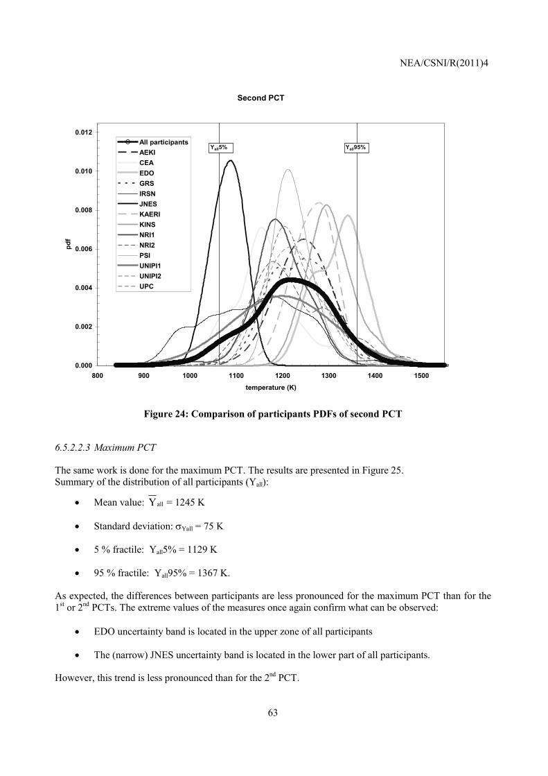
NEA/CSNI/R(2011)4
63
Second PCT
0.000
0.002
0.004
0.006
0.008
0.010
0.012
800 900 1000 1100 1200 1300 1400 1500
temperature (K)
All participantsAEKICEAEDOGRSIRSNJNESKAERIKINSNRI1NRI2PSIUNIPI1UNIPI2UPC
Yall5% Yall95%
Figure 24: Comparison of participants PDFs of second PCT
6.5.2.2.3 Maximum PCT
The same work is done for the maximum PCT. The results are presented in Figure 25. Summary of the distribution of all participants (Yall):
• Mean value: allY = 1245 K
• Standard deviation: σYall = 75 K
• 5 % fractile: Yall5% = 1129 K
• 95 % fractile: Yall95% = 1367 K.
As expected, the differences between participants are less pronounced for the maximum PCT than for the 1st or 2nd PCTs. The extreme values of the measures once again confirm what can be observed:
• EDO uncertainty band is located in the upper zone of all participants
• The (narrow) JNES uncertainty band is located in the lower part of all participants.
However, this trend is less pronounced than for the 2nd PCT.
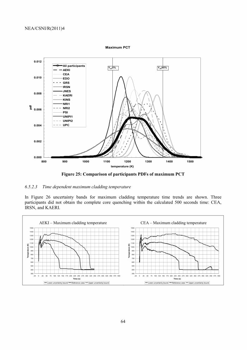
NEA/CSNI/R(2011)4
64
Maximum PCT
0.000
0.002
0.004
0.006
0.008
0.010
0.012
800 900 1000 1100 1200 1300 1400 1500
temperature (K)
All participantsAEKICEAEDOGRSIRSNJNESKAERIKINSNRI1NRI2PSIUNIPI1UNIPI2UPC
Yall5% Yall95%
Figure 25: Comparison of participants PDFs of maximum PCT
6.5.2.3 Time dependent maximum cladding temperature
In Figure 26 uncertainty bands for maximum cladding temperature time trends are shown. Three participants did not obtain the complete core quenching within the calculated 500 seconds time: CEA, IRSN, and KAERI.
AEKI – Maximum cladding temperature
300
400
500
600
700
800
900
1000
1100
1200
1300
1400
1500
-25 0 25 50 75 100 125 150 175 200 225 250 275 300 325 350 375 400 425 450 475 500
Time (s)
Tem
pera
ture
(K)
Lower uncertainty bound Reference case Upper uncertianty bound
CEA – Maximum cladding temperature
300
400
500
600
700
800
900
1000
1100
1200
1300
1400
1500
-25 0 25 50 75 100 125 150 175 200 225 250 275 300 325 350 375 400 425 450 475 500
Time (s)
Tem
pera
ture
(K)
Lower uncertainty bound Reference case Upper uncertianty bound
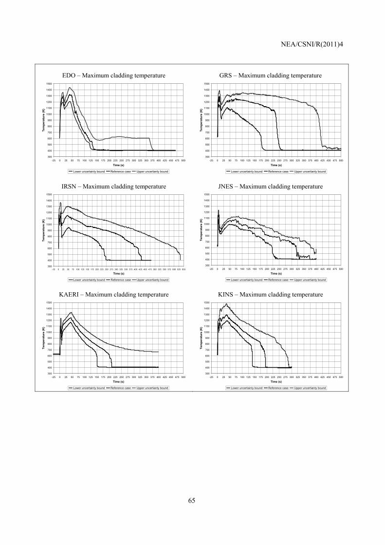
NEA/CSNI/R(2011)4
65
EDO – Maximum cladding temperature
300
400
500
600
700
800
900
1000
1100
1200
1300
1400
1500
-25 0 25 50 75 100 125 150 175 200 225 250 275 300 325 350 375 400 425 450 475 500
Time (s)
Tem
pera
ture
(K)
Lower uncertainty bound Reference case Upper uncertianty bound
GRS – Maximum cladding temperature
300
400
500
600
700
800
900
1000
1100
1200
1300
1400
1500
-25 0 25 50 75 100 125 150 175 200 225 250 275 300 325 350 375 400 425 450 475 500
Time (s)
Tem
pera
ture
(K)
Lower uncertainty bound Reference case Upper uncertianty bound
IRSN – Maximum cladding temperature
300
400
500
600
700
800
900
1000
1100
1200
1300
1400
1500
-25 0 25 50 75 100 125 150 175 200 225 250 275 300 325 350 375 400 425 450 475 500 525 550 575 600 625 650
Time (s)
Tem
pera
ture
(K)
Lower uncertainty bound Reference case Upper uncertianty bound
JNES – Maximum cladding temperature
300
400
500
600
700
800
900
1000
1100
1200
1300
1400
1500
-25 0 25 50 75 100 125 150 175 200 225 250 275 300 325 350 375 400 425 450 475 500
Time (s)
Tem
pera
ture
(K)
Lower uncertainty bound Reference case Upper uncertianty bound
KAERI – Maximum cladding temperature
300
400
500
600
700
800
900
1000
1100
1200
1300
1400
1500
-25 0 25 50 75 100 125 150 175 200 225 250 275 300 325 350 375 400 425 450 475 500
Time (s)
Tem
pera
ture
(K)
Lower uncertainty bound Reference case Upper uncertianty bound
KINS – Maximum cladding temperature
300
400
500
600
700
800
900
1000
1100
1200
1300
1400
1500
-25 0 25 50 75 100 125 150 175 200 225 250 275 300 325 350 375 400 425 450 475 500
Time (s)
Tem
pera
ture
(K)
Lower uncertainty bound Reference case Upper uncertianty bound

NEA/CSNI/R(2011)4
66
NRI1 – Maximum cladding temperature
300
400
500
600
700
800
900
1000
1100
1200
1300
1400
1500
-25 0 25 50 75 100 125 150 175 200 225 250 275 300 325 350 375 400 425 450 475 500
Time (s)
Tem
pera
ture
(K)
Lower uncertainty bound Reference case Upper uncertianty bound
NRI2 – Maximum cladding temperature
300
400
500
600
700
800
900
1000
1100
1200
1300
1400
1500
-25 0 25 50 75 100 125 150 175 200 225 250 275 300 325 350 375 400 425 450 475 500
Time (s)
Tem
pera
ture
(K)
Lower uncertainty bound Reference case Upper uncertianty bound
PSI – Maximum cladding temperature
300
400
500
600
700
800
900
1000
1100
1200
1300
1400
1500
-25 0 25 50 75 100 125 150 175 200 225 250 275 300 325 350 375 400 425 450 475 500
Time (s)
Tem
pera
ture
(K)
Lower uncertainty bound Reference case Upper uncertianty bound
UNIPI1 – Maximum cladding temperature
300
400
500
600
700
800
900
1000
1100
1200
1300
1400
1500
-25 0 25 50 75 100 125 150 175 200 225 250 275 300 325 350 375 400 425 450 475 500
Time (s)
Tem
pera
ture
(K)
Lower uncertainty bound Reference case Upper uncertianty bound
UNIPI2 – Maximum cladding temperature
300
400
500
600
700
800
900
1000
1100
1200
1300
1400
1500
-25 0 25 50 75 100 125 150 175 200 225 250 275 300 325 350 375 400 425 450 475 500
Time (s)
Tem
pera
ture
(K)
Lower uncertainty bound Reference case Upper uncertianty bound
UPC – Maximum cladding temperature
300
400
500
600
700
800
900
1000
1100
1200
1300
1400
1500
-25 0 25 50 75 100 125 150 175 200 225 250 275 300 325 350 375 400 425 450 475 500
Time (s)
Tem
pera
ture
(K)
Lower uncertainty bound Reference case Upper uncertianty bound
Figure 26: Calculated uncertainty bands for maximum cladding temperature
6.5.3 Results of sensitivity analysis
Following the method proposed for BEMUSE phase III described in Chapter 4, the output parameters required for sensitivity ranking are separated into two groups: One related to cladding temperature and the other related to primary pressure. Those output parameters related to the core cladding temperatures are:
• 1st PCT
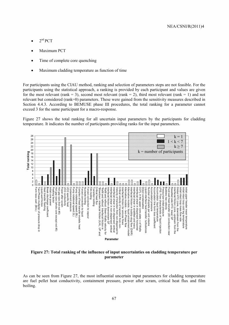
NEA/CSNI/R(2011)4
67
• 2nd PCT
• Maximum PCT
• Time of complete core quenching
• Maximum cladding temperature as function of time
For participants using the CIAU method, ranking and selection of parameters steps are not feasible. For the participants using the statistical approach, a ranking is provided by each participant and values are given for the most relevant (rank = 3), second most relevant (rank = 2), third most relevant (rank = 1) and not relevant but considered (rank=0) parameters. These were gained from the sensitivity measures described in Section 4.4.3. According to BEMUSE phase III procedures, the total ranking for a parameter cannot exceed 3 for the same participant for a macro-response. Figure 27 shows the total ranking for all uncertain input parameters by the participants for cladding temperature. It indicates the number of participants providing ranks for the input parameters.
02468
10121416182022242628
Form loss coef. (B
CL)
Two-P
hase multiplier of pressure drop in
Liquid-wall friction
Heat transfer flashing
Break discharge coefficient
Initial core power
Peaking factor
Hot gap size (w
hole core except rod #5)H
ot gap size (hot rod #5)P
ower after scram
UO
2 conductivity U
O2 specific heat
Containm
ent pressureP
ump rotational speed (IL)
Pum
p rotational speed (BL)
Com
plex of heat transfer models: heat
Forced convection to liquidN
ucleate boilingForced convection to vapourFilm
boilingTransition bolilingC
ritical heat flux*B
lowdow
n: interfacial friction (ILHL, U
P and
*Refill and reflood: Interfacial friction in
*Refill and reflood: S
teen-Wallis velocity for
Interfacial friction downstream
QF
Interfacial shear in non-dispersed verticalInterfacial shear in non-dispersed verticalV
elocity of transition from non-dispersed to
Critical velocity of transition from
non-Interfacial friction for annular flow
sA
lternative models – tw
o-Phase flow
Alternative m
odels: liquid entrainment m
odelInterfacial friction in bubbly-slug flow
(DW
R)
Interfacial shear in stratified and wavy
Interfacial shear in dispersed horizontalC
CFL in the upper core plate: c of W
allisD
irect condensationLiquid-interface heat transfer: turbulencesN
umber of droplets per unit volum
eA
ccumulator:pressure
Accum
ulator line form loss coefficient
Accum
ulator: liqud temperature
LPIS
: Flow characteristic of liquid injection
Pressurizer initial pressure
Bubbles rise velocity
Fluid-wall heat transfer (2D
conduction nearR
ewetted side H
TC: low
er QF
Interfacial friction (core, upstream from
theG
lobal HTC
(core, downstream
from the
Initial intact loop mass flow
rateInitial intact loop cold leg tem
peratureInitial upper header m
ean temperature
Parameter
Tota
l ran
king
Figure 27: Total ranking of the influence of input uncertainties on cladding temperature per parameter
As can be seen from Figure 27, the most influential uncertain input parameters for cladding temperature are fuel pellet heat conductivity, containment pressure, power after scram, critical heat flux and film boiling.
k = 1 1 < k < 7
k ≥ 7 k = number of participants
NEA/CSNI/R(2011)4
68
Figure compares two selected parameters, film boiling heat transfer and critical heat flux, in terms of both, the range of variation and the influence ranking on cladding temperature by the participants. The range of variation of each input parameter is expressed as fraction of the reference value and can be compared among the participants. As for phase III, the coordinator of Phase V compared these two parameters plus forced convection to vapour which do not have the highest total ranking in Figure 27. The range of fuel related parameter values was proposed. As shown in Figure 28 there is not a very clear relationship between range of variation and the influence. The reason is explained in Section 4.4.3.
Some observations from Figure 28:
• The range of variation of CHF considered by IRSN is rather large, whereas this parameter has no influence. It can be partly explained because IRSN defined also uncertainty of the quench front model as highly influential.
• GRS and UPC have similar ranges for the film boiling heat transfer, but GRS finds film boiling as highly influential and UPC not at all. The origin of the difference may be: GRS finds that the choice among two models of film boiling is highly influential but not the multipliers of the models themselves, whereas UPC considers only multipliers. Uncertainty ranges for CATHARE users are much larger than for the rest of participants. This difference may be explained by differences among the codes.
Film boiling heat transfer
0
1
2
3
4
5
6
7
8
9
10
AEKI CEA EDO GRS IRSN JNES KAERI KINS NRI1 NRI2 PSI UPC
Participant
Ran
gew
idth
0
1
2
3
4
5
Ran
king
valu
e
Range width Ranking value
GRS: Dougall-Rohsenow GRS: Condie-Bengston IV IRSN: All phases IRSN: Reflood UPC: Conduction term UPC: Convection term
Critical heat flux
0
0.5
1
1.5
2
AEKI CEA EDO GRS IRSN JNES KAERI KINS NRI1 NRI2 PSI UPCParticipant
Ran
gew
idth
0
1
2
3
4
Ran
king
valu
e
Range width Ranking value
Figure 28: Ranges of variation and influence on cladding temperature for selected input parameters

NEA/CSNI/R(2011)4
69
6.6 Conclusions of Phase V
For uncertainty and sensitivity analysis, all the participants used a statistical method according to the use of Wilks’ formula, except UNIPI applied its CIAU method.
Differences can be seen in the results of different participants with regard to the base case or reference calculations; the largest difference among two participants is 141 K for the maximum PCT, which is lower than in Phase IV (167 K). The largest difference among participants for the maximum PCT in Phase III calculating the LOFT experiment is 151 K. The difference of the upper 95%/ 95% uncertainty range, which is important to compare with the regulatory acceptance criterion, is 221 K for maximum PCT between participants (LOFT calculation: 155 K). The differences between the calculated uncertainty limits and their distance to the base case calculations for maximum PCT are calculated from 53 K (JNES) to 239 K (NRI2). Two participants of the statistical method used only the 20 common parameters, one used only 17 parameters, and the others included several model parameters what obviously caused differences in uncertainty results. Other differences may be due to differences of ranges of input uncertainties defined by the participants.
The difference in results comparing the upper 95%/95% bound of the two peak cladding temperatures between 1st order (59 calculations) and 4th order (153 calculations) performed by GRS with the ATHLET code is 40 K and 78 K for the 1st PCT and 2nd PCT, respectively [20]. Input uncertainty selection and quantification of uncertainty distributions and especially ranges are more important for the uncertainty ranges of the output than the number of calculations with the aim to increase the order of Wilks’ formula.
Although the overall results are clearly a step forward towards the consolidation of the different methods, the uncertainty bands for the single-valued output parameters, which do not show agreement among the participants in general, and specifically among users of the statistical approach, may point out that for the last approach, the uncertainty analyses have not been very well mastered by some participants.
The calculated uncertainty bands for both the 1st and the 2nd peak cladding temperatures show no overlap among the results of the participants. For the “maximum peak cladding temperature” (single value), the dispersion of the band width is significantly less for the statistical methods, and there is a region of overlap of about 15 K. The missing overlap can be explained by quite different best-estimate calculations combined with rather narrow uncertainty bands. The emphasis on uncertainty analysis, however, is to quantify lack of precise knowledge by appropriate uncertainty ranges of input parameters, what was obviously not the case in all applications. Although it was not a main goal of the exercise, it is worth mentioning that the upper (95%/95%) limit estimations for maximum PCT by the participants do not exceed the regulatory acceptance limit 1477 K, but two participants are close to this limit.
For selecting the uncertain input parameters to be used generally the recommendations were followed to use the common uncertainties and their distributions. Three participants, however, considered only the agreed common set of proposed parameters without including uncertainties of code models. Ranges and distributions of code model parameters are still different even among users of the same code. These were obviously primarily specified by engineering judgement.
Sensitivity analysis has been successfully performed by all participants using the statistical method. The influence ranking has been estimated for two macro responses: Cladding temperature and primary pressure. The sensitivity coefficients used by participants are Pearson and Spearman correlation

NEA/CSNI/R(2011)4
70
coefficient, standardised rank regression coefficients, Pearson and Spearman partial correlation coefficients and SOBOL indices.
The sensitivity results have shown that several parameters were ranked as influential by the majority of the 12 participants. These quantities are:
• From the set of common uncertain parameters: “Power after scram” (12 participants out of 12 – 12/12) and “UO2 conductivity” (11/12) for the cladding temperature; “Containment pressure” (10/12), “Initial ILCL temperature” (9/10) and “Initial upper head temperature” (6/8) for the primary pressure.
• From the individually determined input parameters: “Film boiling” (6/8) and “Critical heat flux” (7/9).
BEMUSE phase V helped clarifying the treatment of failed calculations and its relation to the number of runs for participants using statistical methods to provide 95%/95% statements. All participants followed the recommendation stated in phase III to increase the number of code runs in order to compensate for failed runs (see Section 6.4 and next chapter of this report). In one case, more code runs were omitted in spite of corrections of the maximum time step size.

NEA/CSNI/R(2011)4
71
7. CONCLUSIONS AND RECOMMENDATIONS
7.1 Uncertainty methods and computer codes used
The BEMUSE activity compared the applications of essentially two uncertainty methods. The first method uses a probabilistic approach which propagates input uncertainties to the output uncertainties. The method is associated with order statistics and the use of Wilks’ formula. That method was first proposed by GRS, and applied by the majority of participants. The second method is the Uncertainty Method based on Accuracy Extrapolation (UMAE) and its extension to the Code with the Capability of Internal Assessment of Uncertainty (CIAU). A comparison of calculation results with data from integral experiments investigating the same course of event for which the uncertainty analysis is to be performed, is a necessary basis for applying this method. 9 out of 10 participants in phase III and 12 out of 14 participants used the statistical method in Phase V, only University of Pisa used their own method in the BEMUSE programme. A reason is the high effort needed to get the data base for deviations between experiment and calculation results in CIAU. That time and resource consuming process has been performed only by University Pisa for the codes CATHARE and RELAP. The data base is available only there.
Different computer codes were applied by the different participants using these methods. A direct comparison between both applications of the above mentioned methods (CIAU and GRS) can only be seen for applications of the CATHARE and RELAP5 codes. However, each participant used different nodalisations and partly different code options. Therefore, comparisons of both uncertainty methods in this Programme are influenced by user specific applications of a computer code or by using different computer codes. However, the BEMUSE applications allow to see different applications of two uncertainty methods. The statistical methods were applied differently by those participants using that method.
The decision for an uncertainty method is usually based on the features of a method. The choice of selecting an uncertainty method depends on what the end users will accept and in what features they are interested.
The Pisa Method can be used if:
− Stringent criteria on data and modelling accuracy are met;
− End users accept assumptions about extrapolation of differences between calculation and experimental data from small scale experimental facilities to large scale;
− The last point is most likely to be the case when extrapolation to the case of interest is small.
This method requires having a sufficient data base, which represents an outstanding amount of work. Besides, it does not provide tolerance limits, like confidence level of the provided upper and lower bounds. Additional calculations with respect to those performed for the determination of uncertainty bounds are

NEA/CSNI/R(2011)4
72
necessary to get information on sensitivities of input uncertainties, like fuel parameters, which are usually not available from integral system experiments.
Statistical methods can be used if:
− End users accept the method based on estimation of probability distributions of input parameters, what is the most important part to come up with well justified distributions and ranges;
− Users are interested in sensitivity measures to help prioritize future improvements;
− Users are not interested to limit the number of input uncertainties because the number of code calculations to be performed is independent of the number of uncertainties.
In all cases appropriate knowledge, skill, experience and quality standards must be applied. One important result is that the quality of base case calculation is essential as a basis for uncertainty results. A necessary pre-requisite is a well qualified computer code which is suitable to calculate the course of event under investigation.
For those participants using a statistical method with Wilks’ formula one can state common features and differences. Common is the use of simple random sampling as it is advisable for the use of Wilks’ formula. Differences are in the number of calculations (order of Wilks’ formula), the list of input parameters, and the type of distribution of parameter values, their ranges, and the treatment of failed calculations.
Since most of the participants used the statistical method the following conclusions and recommendations are mainly dealing with this approach.
7.2 Number of uncertain input parameters, determination of distributions and selection of values from their distributions
The number of uncertain input parameters ranges from 13 to 64 in BEMUSE phase III, and from 17 to 55 in phase V. The main reason to consider only a limited number of parameters is the difficulty to associate with them an appropriate range and distribution of variation. However, significant sources of uncertainty should not be omitted.
Some participants restricted the uncertain input parameters to the agreed common list in phase V, some excluded break discharge parameters due to the recommendation not to vary discharge flow cross section.
Concerning the number of input parameters, a compromise should be found among the following considerations:
- In uncertainty analysis, Wilks’ formula makes it possible to consider a high number of input parameters.
- Consideration of model parameter uncertainties may be difficult because access via input decks is needed.
- A high number of input parameters needs high effort to define the uncertainty distributions.

NEA/CSNI/R(2011)4
73
- In sensitivity analysis, the results are more reliable if the number of code runs is significantly higher than the number of input parameters. However, one is usually only interested in the most influential input parameters with regard to code output parameters.
One of the most important steps in applying a statistical method is the determination of ranges and distributions of the uncertain parameter values. The important parameters have significant influence on the uncertainty ranges of the results. The quantification of the input uncertainty is to be performed by different sources of information: 1) Validation of mainly separate effects experiments, partly integral experiments,
2) Expert judgement,
3) Literature, e.g. measurement uncertainties of correlations of heat transfer, friction, pressure losses, etc.
Experience from code validation is the main basis to determine code model uncertainties. This is mainly performed by experts performing the validation. Appropriate experimental data are needed. Focusing further investigations on the issue of input parameters would be desirable. In some cases, methods of statistical analysis of experimental data compared to code results should be applied, for instance by the code developers. Formal methods, like Bayesian and Maximum Entropy methods, can be used to help to specify probability distributions for model parameters. In other cases expert judgement is used. A good knowledge of the experts who performed code validation is necessary to provide these judgements.
A comparison of calculated uncertainties with experimental data is recommended also for another reason. It allows checking not only the appropriate mathematical formulation of the physical models but also their implementation in the code, what is not the case with uncertainties found in literature.
It is also important to note that the model outcome sample values y1,…,yN from which the tolerance intervals/limits are determined must constitute a random sample of the model outcome Y in the statistical sense, i.e. they must be realizations of stochastically independent and identically distributed random variables Y1,….,YN. This is ensured if the underlying input parameter sample is generated according to the simple random sampling (SRS) principle. Other types of parameter selection procedures like “Latin-Hypercube-Sampling” or “Importance-Sampling” etc. may therefore not be appropriate for tolerance intervals or tolerance limits.
7.3 Uncertainty results
The calculation results of the differences of upper uncertainty limits minus base calculation by participants for PCT lie in the range from 28 K to 207 K, and from 53 K to 239 K in phases III and V, respectively. The results using the CIAU method are comparable to those of other participants for phase III, for phase V larger uncertainty bands were calculated for peak cladding temperature. The calculation results for pressure in phases III and V show low widths of the uncertainty bands for the statistical methods. The uncertainty bands of the CIAU results are much larger than those of the other participants in phases III and V. This is explained by the time uncertainty included in the bands of the CIAU method. CIAU approximates the time error on the basis of comparing experimental data and calculations. The various experiments have different time constants.
Using the CIAU method, the uncertainty bands derived from Total Quantity Uncertainty (TQU) provide higher values for maximum and minimum values of the uncertainty bands of cladding temperatures than the statistical methods. Smaller band widths are generated by considering Quantity Uncertainties (QU) only what is more appropriate to compare peak cladding temperature values with the statistical methods.

NEA/CSNI/R(2011)4
74
QU values were used for comparison of PCT values in phase V. In phase III only TQU band width were used for comparison. The TQU band width in Phase III calculating the LOFT experiment are lower at the time when the PCTs are occurring than those in the Zion NPP calculations.
For phase III, two main reasons were given if the upper and lower bounds do not envelop the experimental data: Deviation of the reference calculation from experimental data, and too narrow uncertainty bands for the uncertain input parameters. A further reason may be missing influential uncertain input parameters. Some participants concentrated mainly on the cladding temperature when identifying the uncertain input parameters.
The elicitation and quantification process of input uncertainties is a basis for performing an uncertainty analysis using a statistical method. The input uncertainty ranges determine the uncertainties of the code calculation results, i.e. the output uncertainties. If important input uncertainties are not included, the result can only give an answer to the selected parameters. Comparing the different submissions of phase V, for example, one should take into account that not all participants included model uncertainties of the applied computer code.
A change of the type of distribution of input uncertainties (for example, uniform instead of normal, with similar ranges of variations) has a relative low influence on the upper tolerance limit of cladding temperature compared to the differences of base case calculation results and to differences of input uncertainty ranges.
7.4 Influence or sensitivity results
Influence or sensitivity analysis results can give guidance to select the important variables, for which the uncertainty distribution has to be determined with good accuracy. These sensitivity results are approximately the same for the dominant parameters irrespective of the number of calculations performed, i.e. the order of Wilks’ formula. However, the number of calculations should be larger than the number of uncertain input parameters in order to get reliable sensitivity measures for the dominant parameters. Pearson’s and Spearman’s correlation coefficients used as sensitivity measures give the same ranking for the important parameters.
Since in reactor safety analyses very often extremely complex and computationally expensive models are used, it is clear that in most cases additional model runs only for the purpose of sensitivity analysis will not be affordable. Thus, the selection of sensitivity/influence/ importance indices must be restricted to those which can be computed from the available sample values already generated for uncertainty analysis, i.e. from the simple random sample (SRS) generated to determine non-parametric tolerance limits. Suitable/feasible indices in such cases are e.g. the standard correlation/regression/R2-based indices, their rank-based counterparts and the Correlation Ratio (= 1st order Sobol’s variance-based sensitivity index) and some others computed from the available SRS-sample values. Sensitivity/influence/importance indices that require additional specific sampling and computational effort like Fourier Amplitude Sensitivity Test (FAST) - indices or the full range of Sobol indices [21] cannot be used in such cases. Therefore it is not intended to provide full, complete and precise sensitivity information with respect to all parameters and all possible outcomes. It rather seems sufficient and satisfactory to identify only the dominating uncertain parameters, i.e. those few with the highest impact/influence on the output uncertainty. Experience shows that in most practical applications dominating uncertainties can be found with the simplest standard sensitivity indices like Correlation Coefficients (CC/RCC) or Correlation Ratio, and at the low sampling/computational cost from uncertainty analysis with non-parametric tolerance limits. Additional model runs are not necessary in most cases.

NEA/CSNI/R(2011)4
75
Nevertheless, it is clear that more accurate and more exhaustive sensitivity information can be obtained in situations where the size of the sample does not play any role, e.g. with variance-based Sobol or FAST indices. However, the extremely large number of model runs required by these procedures makes them impracticable for computationally demanding models.
7.5 Treatment of failed runs
For a proper use of Wilks’ formula, all the code runs must be successful, or corrected in case of failure. This requirement becomes more and more difficult when the number of code runs increases. A failed run from which the result of interest (e.g. PCT) cannot be reproduced nor estimated or bounded, it may be assumed conservatively that the result from this run will exceed all the results from the completed runs. Thus, according to “Wilks’ 95%/95%-formula”, the sample size must correspondingly be increased. For one failed run at least 93-1=92 correct runs are needed and the highest value of the output obtained with the 92 successful code runs is retained, for two failed at least 124-2=122 correct and in the same way, the highest value obtained with the 122 successful code runs is retained, for three failed at least 153-3=150 correct, for four failed at least 181-3=177, etc.
It is, however, possible to check the evolution of the parameter values of interest in the failed runs. If, until the code failure occurs, these values are within the band of the successful runs, then this run can be regarded as successful. When PCT is of interest, and the run failure occurred well after the time of PCT, and the PCT value of the failed run is within the uncertainty band, the failed run can be considered successful with regard to PCT.
If the failure occurred due to a too large time step in a trouble zone, like subcooled ECC injection, what was the main reason, and the time step was reduced, the run could be continued after time step reduction. In such a case, the run is to be considered successful. An appropriate automatic time step control by the code could have prevented the run failure.
7.6 Statistical convergence of tolerance limits
When the upper tolerance limit approaches regulatory acceptance criteria, e.g. 1200°C PCT, the number of code runs may be increased to 150 or 200 calculations instead of the 59 code runs needed, using Wilks’ formula at the first order for the estimation of a α = 95% one-sided tolerance limit with a confidence level β of 95%. This would be advisable for two reasons:
1) With increasing sample size the uncertainty results will be less dispersed, and consequently more converged (less conservative), and
2) The sensitivity results will be more reliable.
Firstly, for uncertainty analysis, it is possible to use Wilks’ formula for example at the order 3 (124 runs) up to 5 (181 runs) for percentile α and confidence β unchanged, which may reduce the effect of conservatism of tolerance limits from a small number of code runs, i.e. the dispersion of the estimated tolerance limit in conservative direction tending to substantially overestimate the 95%-quantile one is originally interested in. On the other hand, the underestimation of the 95% percentile with 5% probability decreases when the order of Wilks’ formula is increased.
Secondly the results of sensitivity analysis will become more reliable, particularly for less important parameters, because the variances of the estimators of the sensitivity measures will decrease and spurious (artificial) correlations between independent input parameters will appear less frequently when sample sizes increase. The issue of the number of code runs required for a proper sensitivity analysis is
NEA/CSNI/R(2011)4
76
independent of that required by Wilks’ formula. For example and unlike Wilks’ formula, mainly for Regression Coefficients, the number of code runs should be (significantly) higher than the number of input parameters.
The USNRC Regulatory Guide 1.157 [7] requires that the applicable acceptance criteria will not be exceeded with a probability of 95% or more. If an additional confidence level is provided, the IAEA SSG-2 [11] requires at least 95%. Therefore, an overestimation of the 95% percentile with 95% probability would be in line with requirements of these guides. An upper bound close to the theoretical 95% percentile is not required for licensing applications because the percentile may be higher than 95%.
It is important to note that differences up to 50 K for PCT found in Phase III or up to 80 K for Phase V results by changing the number of calculations from 59 up to 1003 (or from 93 to 153 runs) are low compared with the highest differences between results of participants for the reference calculations of 141 K, and the upper uncertainty range of maximum PCT up to 221 K in Phase V. One should also note the maximum difference of calculated maximum PCT of participants in Phase IV was 103 K, e.g. for the lower range of maximum linear power using the same values for that input parameter. A reason for this difference of results may be different models for the same heat transfer regime in different codes, different changes of heat transfer regimes during the transient due to different nodalisations and due to other selections in the input decks.This shows clearly the high importance for the need of high quality results of the base calculation, selection of uncertain input parameters, and the variation of input parameters over their uncertainty ranges on the uncertainty of code output parameters rather than the number of calculations.
Another way to reduce the over-estimation of the 95% percentile by 95%/95% tolerance limits is to assume a distribution of the output variable, e.g. normal distribution, and to check the distribution by a suitable statistical test. In these cases one obtains less conservative bounds with the same number of calculations, or the same conservatism with a lower number of calculations, e.g. instead of 59 runs only 24 are necessary or instead of 181 runs only 83 are needed [22]. Such a procedure was not part of the BEMUSE programme.
In the Bootstrap method re-sampling [17] using the original parameter selections is performed. The procedure leads to lower limits than the Wilks’ tolerance limit. However, the method is not recommended because the 95%/95% criterion is not necessarily fulfilled, at least for low number of calculations, like 59 runs [22].
7.7 Lessons learned
The main lessons learned from all the exercises performed in the BEMUSE programme, especially from phases III and V are:
• A qualified user is needed to perform a high quality reference calculation, i.e. qualified nodalisation, appropriate initial and boundary conditions, selections of code options; quality assurance procedures should be followed.
• A suitable code and uncertainty method should be used.
When applying the statistical method (first proposed by GRS), the following items are important:
• The identification and quantification of potential important uncertain input parameters is fundamental, i.e. phenomena, code models, initial and boundary conditions, material, like fuel parameters. Figures 5 and 27 as well as Table 8 is useful in this regard. Such a table would also be beneficial for other events than large break LOCA.

NEA/CSNI/R(2011)4
77
• More emphasis should be on quantification of input uncertainties of code models using validation experience.
• The important input parameters that affect the course of the event should be clear to the user and the reviewer of an application.
• Simple random sampling (SRS) should be used to derive tolerance intervals or one-sided tolerance limits.
• The convergence towards the 95% quantile, for example, is increased by an increased number of code runs. The dispersion of tolerance limits is reduced by an increased number of code runs.
• The 95%/95% tolerance limit should meet the regulatory acceptance criterion. If the calculated tolerance limit approaches the acceptance criterion, the number of code runs may be increased.
The code runs with the randomly selected values of uncertain input parameters should end successfully. When PCT is of interest, and a run fails after the time of PCT, the failed run can be considered successful with regard to PCT. Otherwise, the number of code runs should be increased in order to compensate for failed runs (see Sections 6.4 and 7.5 of this report).
7.8 General remarks
The methods used in this activity are considered to be mature for application, including licensing processes. Lessons learned for a proper application of the statistical method are listed in the previous section as result of the performed exercise. Differences are observed in the application of the methods, consequently results of uncertainty analysis of the same task lead to different results. These differences raise concerns about the validity of the results obtained when applying uncertainty methods to system analysis codes. The differences may stem from the application of different codes and uncertainty methods. In addition, differences between applications of statistical methods may mainly be due to different input uncertainties, their ranges and distributions. Differences between CIAU applications may stem from different data bases used for the analysis. However, - as it was shown by BEMUSE phases III and V - significant differences were observed already between the base or reference calculation results. Furthermore, differences were seen in the results using the same values of single input parameter variations in BEMUSE phases II and IV.
When a conservative safety analysis method is used, it is claimed that all uncertainties which are considered by an uncertainty analysis are bounded by conservative assumptions. Differences in calculation results of conservative codes would also be seen due to the user effect such as different nodalisation and code options, like for best estimate codes used in the BEMUSE programme. Differences of code calculation results have been observed for a long time, and have been experienced in all International Standard Problems where participants calculated the same experiment or a reactor event [23]. The main reason is that the user of a computer code has a big influence on how a code is used. The objective of an uncertainty analysis is to quantify the uncertainties of a code result. An uncertainty analysis can not compensate for code deficiencies. Therefore, necessary pre-condition is that the code is suitable to calculate the scenario under investigation.
A user effect can also be seen in applications of uncertainty methods, like in the BEMUSE programme. In uncertainty analysis, the emphasis is on the quantification of a lack of precise knowledge by defining appropriate uncertainty ranges of input parameters, which could not be achieved in all cases in BEMUSE. For example, some participants specified too narrow uncertainty ranges for important input uncertainties based on expert judgement, and not on sufficient code validation experience. Therefore, skill, experience and knowledge of the users about the applied suitable computer code as well as the used uncertainty method are important for the quality of the results.

NEA/CSNI/R(2011)4
78
Instead of emphasising too much an appropriate number of calculations to be performed when applying the statistical method, one should concentrate first on the basis or reference calculation. However, an increased number of calculations may be advisable because it decreases the dispersion of the tolerance limits. Secondly, it is very important to include influential parameters and provide distributions of uncertain input parameters, mainly their ranges. These assumptions must be well justified. An important basis to determine code model uncertainties is the experience from code validation. This is mainly provided by experts performing the validation. Appropriate experimental data are needed. More effort, specific procedures and judgement should be focussed on the determination of input uncertainties.
This last point is an issue for recommendation for further work. Especially, the method used to select and quantify computer code model uncertainties and to compare their effects on the uncertainty of the results could be studied in a future common international investigation using different computer codes. That may be performed based on the same experiments. Approaches can be tested to derive these uncertainties by comparing calculation results and experimental data. Other areas are selection of nodalisation and code options. This issue on improving the reference calculations among participants is fundamental in order to obtain more common uncertainty bands of the results.
NEA/CSNI/R(2011)4
79
REFERENCES
[1] B. Boyack, et al.: “Quantifying Reactor Safety Margins; Nuclear Engineering and Design 119, pp.1-95, 1990.
[2] H. Glaeser, E. Hofer, M. Kloos, T., Skorek: “Uncertainty and Sensitivity Analysis of a Post-Experiment Calculation in Thermals Hydraulics”; Reliability Engineering and System Safety, Vol. 45, pp. 19-33, 1994.
[3] S.S. Wilks: “Statistical Prediction with Special reference to the Problem of Tolerance Limits”; Annals of Mathematical Statistics, vol. 13, no.4, pp. 400-409, 1942.
[4] F. D’Auria, N. Debrecin, G. M. Galassi: “Outline of the Uncertainty Methodology based on Accuracy Extrapolation (UMAE)”, J. Nuclear Technology, Vol. 109, No 1, pg. 21-38, 1995.
[5] F. D’Auria, W. Giannotti: “Development of Code with capability of Internal Assessment of Uncertainty”, J. Nuclear Technology, Vol. 131, No 1, pg. 159-196, August 2000.
[6] 10 CFR 50.46, “Acceptance criteria for emergency core cooling systems for light water nuclear power reactors,” Appendix K, “ECCS Evaluation Models”, to 10 CFR Part 50, Code of Federal Regulations, 1996
[7] Regulatory Guide 1.157: “Best Estimate Calculations of Emergency Core Cooling System Performance”, U.S. Nuclear Regulatory Commission, Washington, DC, May 1989
[8] Regulatory Guide 1.203: “Transient and Accident Analysis Methods”, U.S. Regulatory Commission, Washington, DC, December 2005
[9] “Accident Analysis for Nuclear Power Plants”, Safety Report Series 23, International Atomic Energy Agency, Vienna 2002
[10] “Best Estimate Safety Analysis for Nuclear Power Plants: Uncertainty Evaluation”, Safety Report Series 52, International Atomic Energy Agency, Vienna 2008
[11] “Deterministic Safety Analysis for Nuclear Power Plants”, Specific Safety Guide No. SSG-2, International Atomic Energy Agency, Vienna 2009
[12] “Report on the Uncertainty Methods Study”, Vols. I and II, Committee on the Safety of Nuclear Installations, Nuclear Energy Agency, NEA/CSNI R(97) 35, June 1998.
[13] Presentation a priori of the uncertainty evaluation methodology to be used by the participants; NEA/SEN/SIN/AMA(2005)1.
[14] “BEMUSE phase II Report”, Re-analysis of the ISP-13 Exercise, Post Test Analysis of the LOFT L2-5 Test Calculation; NEA/CSNI/R(2006)2, May 2006.
[15] “BEMUSE phase III Report”, Uncertainty and Sensitivity Analysis of the LOFT L2-5 Test; NEA/CSNI/R(2007)4, October2007.
[16] H.A. David, H. N. Nagaraja: “Order Statistics”; Wiley-Interscience, 2003
[17] B. Efron, R.J. Tibshirani: “An introduction to the Bootstrap”; Chapman and Hall, 1993
[18] “BEMUSE phase IV Report”, Simulation of a LB-LOCA in Zion Nuclear Power Plant; NEA/CSNI/R(2008)6, November 2008.

NEA/CSNI/R(2011)4
80
[19] “BEMUSE phase V Report”, Uncertainty and Sensitivity Analysis of a LB-LOCA in Zion Nuclear Power Plant; NEA/CSNI/R(2009)13, December 2009.
[20] T. Skorek: “Uncertainty and Sensitivity Analyses of Experiments and NPP Accidents: Large Break LOCA at Cold Leg of Zion Nucler Power Plant and Comparison with LOFT Test L2-5”; 13th International Topical Meeting on Nuclear Reactor Thermal Hydraulics (NURETH-13), Kanazawa City, Ishikawa Prefecture, Japan, September 27-October 2, 2009
[21] A. Saltelli et al.: Sensitivity Analysis, John Wiley & Sons Ed., 2000
[22] H. Glaeser, B. Krzykacz-Hausmann, W. Luther, S. Schwarz, T. Skorek: “Methodenentwicklung und exemplarische Anwendungen zur Bestimmung der Aussagesicherheit von Rechenprogrammergebnissen”; GRS-A-3443, November 2008
[23] S.N. Aksan, F.D’Auria, H. Städtke: “User Effects on the Transient System Code Calculations”; NEA/CSNI/R(94)35, January 1995
NEA/CSNI/R(2011)4
81
ABBREVIATIONS
AEAT Atomic Energy Authority Technology (United Kingdom) AEKI Hungarian Academy of Sciences KFKI Atomic Energy Research Institute BEMUSE Best Estimate Methods Uncertainty and Sensitivity Evaluation BCL Broken Cold Leg BHL Broken Hot Leg BL Broken Loop CCFL Counter Current Flow Limitation CDF Cumulative Distribution Function CEA Commissariat à l’Energie Atomique (France) CHF Critical Heat Flux CIAU Code with the Capability for Internal Assessment of Uncertainty CIPSU Common Input Parameters associated with a Specific Uncertainty CEA Commissariat à l’Energie Atomique (France) DPCT Difference of Peak Cladding Temperature DC Downcomer EDO Experimental and Design Organisation “Gidropress” (Russia) ENUSA Empresa Nacional del Uranio, SA (Spain) EPRI Electric Power Research Institute (USA) GRS Gesellschaft für Anlagen- und Reaktorsicherheit mbH (Germany) HPIS High Pressure Injection System HS Heat Structures HTC Heat Transfer Coefficient ICL Intact Cold Leg IL Intact Loop ILCL Intact Loop Cold Leg IRSN Institut de Radioprotection et de Sûreté Nucléaire (France) ISP International Standard Problem JNES Japan Nuclear Energy Safety (Japan) KAERI Korea Atomic Energy Research Institute (South Korea) KINS Korean Institute of Nuclear Safety (South Korea) LB-LOCA Large Break Loss Of Coolant Accident LN Log Normal LPIS Low Pressure Injection System LUB Lower Uncertainty Bound MCT Maximum Cladding Temperature MPCT Maximum Peak Cladding Temperature N Normal NRI Nuclear Research Institute Rez (Czech Republic) PCC Partial Correlation Coefficient PCT Peak Cladding Temperature pdf Probability Density Function PIRT Phenomena Identification and Ranking Table PSI Paul Scherrer Institute (Switzerland) PWR Pressurized Water Reactor PZR Pressurizer QF Quench Front RC Reference Case SCC Spearman Correlation Coefficient

NEA/CSNI/R(2011)4
82
PDF Probability Density Function SRRC Standardized Rank Regression Coefficient SRS Simple Random Sampling U Uniform UH Upper-head UMAE Uncertainty Method based on Accuracy Extrapolation UNIPI Università di Pisa UP Upper Plenum UPB Upper Uncertainty Bound UPC Universitat Politècnica de Catalunya (Spain)

NEA/CSNI/R(2011)4
83
APPENDIX 1: FURTHER EVALUATION OF RESULTS FROM BEMUSE PHASE V
P. Bazin (CEA, France)
The objective of this work, performed by CEA, is to compare the results of the uncertainty analysis provided by all the participants during the Phase V of BEMUSE. Each participant provided the uncertainty results in terms of lower bound (LUB) and upper bound (UUB). The idea is to use more complete results than the uncertainty bounds which are extreme values by an estimation of the probability density function (pdf) or cumulative density function (cdf) describing these uncertainties. For technical reasons, only the single-valued output parameters are evaluated here. Among these output parameters, only the values of peak cladding temperature are treated (1st PCT, 2nd PCT and Maximum - in time and space - PCT).
The uncertainty of the output “time of complete core quenching” treatment is possible but not included in this report.
The uncertainty of the output “time of accumulator injection” shows clearly 2 populations, one for the statistical method users, with a very narrow band and one for the CIAU users, with a broad band. This situation is not suitable for a statistical treatment.
The method is detailed for the first PCT and then, applied for 2nd PCT and maximum PCT.
A1-1 First PCT
First step: Building the probability distribution for each participant: For participant using a propagation process (12/14), then (from 90 to 300)1 values of the response (first PCT) are used to build the classical empirical distribution function. For other participants (CIAU methods), the probability law of the uncertainty is assumed to be a normal law with a mean value = (UUB-LUB)/2 and a standard deviation = (UUB-LUB)/4.2 Second step: Clustering of the data of all participants is represented by a CDF representing all the participations. The empirical distribution of all (Yall) participations is built by a random re-sampling using the same amount (10000) of data from each participant (that means, each participant has the same weight).
1 In the case of AEKI, due to the lack of ni code run results for the single-valued output parameters, the same method
as used for UNIPI1 and UNIPI2 is applied. 2 In the case of the CIAU users, i.e. UNIPI1 and UNIPI2, instead of the original UUB and LUB values obtained from
the TQU values, the so-called QU values are used (Table 18 of the BEMUSE phase 5 report or Table 9 of this report).
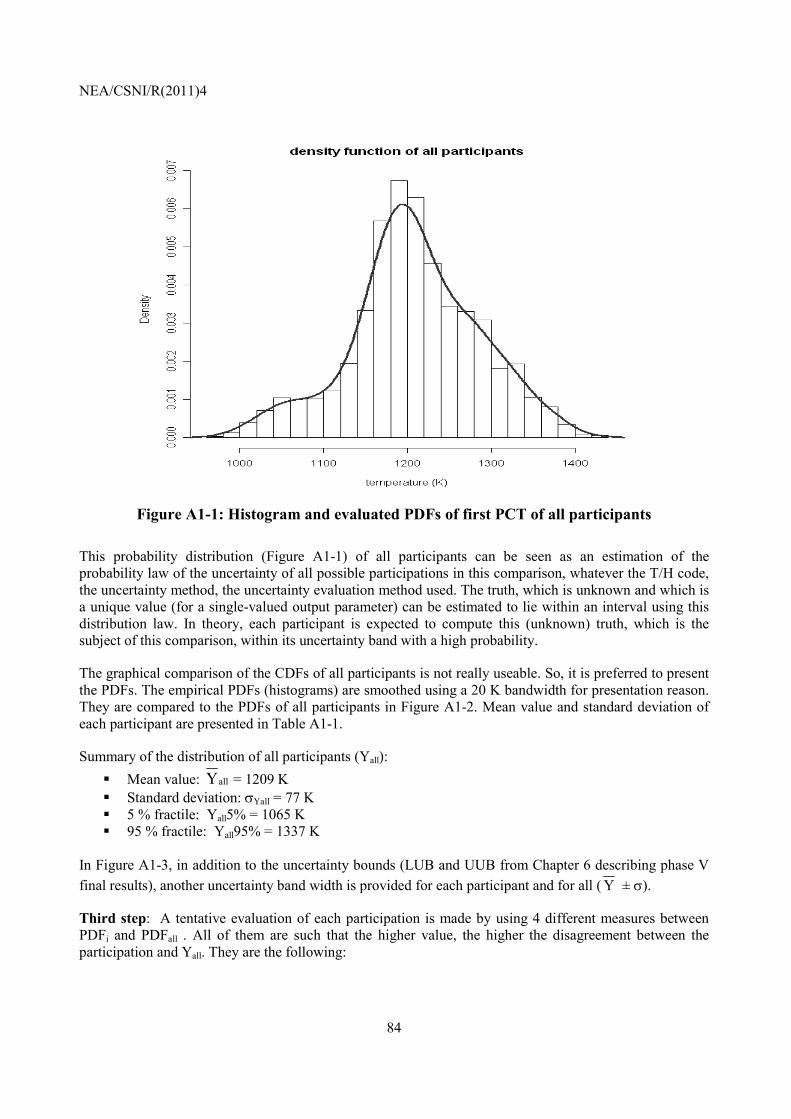
NEA/CSNI/R(2011)4
84
Figure A1-1: Histogram and evaluated PDFs of first PCT of all participants
This probability distribution (Figure A1-1) of all participants can be seen as an estimation of the probability law of the uncertainty of all possible participations in this comparison, whatever the T/H code, the uncertainty method, the uncertainty evaluation method used. The truth, which is unknown and which is a unique value (for a single-valued output parameter) can be estimated to lie within an interval using this distribution law. In theory, each participant is expected to compute this (unknown) truth, which is the subject of this comparison, within its uncertainty band with a high probability.
The graphical comparison of the CDFs of all participants is not really useable. So, it is preferred to present the PDFs. The empirical PDFs (histograms) are smoothed using a 20 K bandwidth for presentation reason. They are compared to the PDFs of all participants in Figure A1-2. Mean value and standard deviation of each participant are presented in Table A1-1.
Summary of the distribution of all participants (Yall): Mean value: allY = 1209 K Standard deviation: σYall = 77 K 5 % fractile: Yall5% = 1065 K 95 % fractile: Yall95% = 1337 K
In Figure A1-3, in addition to the uncertainty bounds (LUB and UUB from Chapter 6 describing phase V final results), another uncertainty band width is provided for each participant and for all ( Y ± σ).
Third step: A tentative evaluation of each participation is made by using 4 different measures between PDFi and PDFall . All of them are such that the higher value, the higher the disagreement between the participation and Yall. They are the following:
NEA/CSNI/R(2011)4
85
• Dimensionless distance: dd1 = 22
2)(
YallYi
alli YYσσ +
−, which is a distance between the mean value between
participant n° i and all, divided by a quadratic sum of the standard deviations.
• Dimensionless distance: dd2 = YallYi
alli YY
σσ +
− which is an absolute value of the difference of the mean
value between participant n° i and all, divided by the sum of the standard deviations.
• Kullback-Leibler divergence: dxxpdfxpdfxpdfpdfpdfD
i
allalliallKL ∫
∞+
∞−
=
)()(log).(),( is a
classical measure of similarity between one probability law and a reference law (all in this case).
• The proportion of probability of participant n° i outside the 90 % confidence interval of all: P(Yi) =
1- ∫%95
%5)(all
all
Y
Y i dxxpdf
By definition, P(Yall) = 0.10. The higher this value is the less the law of participant n° i covers the 90 % confidence interval of all.
The numerical values of these measures can be found in Table A1-1. As a conclusion, no one of these “measure” is really an evaluation of the default or quality of one participant, because a participant is not expected to have the same probability law than this obtained for all (that is also why the DKL is not really adapted). They do not provide either a threshold that could “discard” a particular participant, but the extreme values generally confirm what can be observed in Figures A1-2 or -3, or the simple facts that:
• UNIPI-1: the UUB (1116 K) value is significantly lower than the mean value given by all participants (1209 K)
• EDO: the LUB (1212 K) value is greater than the mean value given by all participants (1209 K). These conclusions are also consistent with the comparison of the LUB, UUB band width of Section 6.5.

NEA/CSNI/R(2011)4
86
Table A1-1: First PCT uncertainty comparison of participants
LUB RC UUB Y
σY dd1 dd2 DKL P(i)
AEKI 1139 1216 1295 1217 39 0.1 0.1 0.9 0.00 CEA 1168 1252 1326 1240 40 0.4 0.3 1.4 0.02 EDO 1212 1306 1382 1302 36 1.1 0.8 4.9 0.17 GRS 1190 1293 1393 1295 55 0.9 0.7 2.1 0.22 IRSN 1142 1218 1379 1259 67 0.5 0.4 0.6 0.13 JNES 1075 1185 1234 1164 35 0.5 0.4 2.1 0.01 KAERI 1129 1187 1237 1186 27 0.3 0.2 2.7 0.00 KINS 1178 1244 1375 1248 45 0.4 0.3 1.6 0.04 NRI1 1046 1191 1299 1175 66 0.3 0.2 0.2 0.06 NRI2 1080 1189 1374 1211 80 0.0 0.0 0.3 0.10 PSI 1131 1178 1237 1181 26 0.3 0.3 2.4 0.00 UNIPI12 991 1054 1116 1054 31 1.9 1.4 13.4 0.61 UNIPI22 1156 1204 1252 1204 24 0.1 0.0 2.2 0.00 UPC 1069 1187 1324 1189 65 0.2 0.1 0.1 0.03 All 1209 77 0 0 0 0.10
First PCT
0.000
0.002
0.004
0.006
0.008
0.010
0.012
900 1000 1100 1200 1300 1400 1500
temperature (K)
All participantsAEKICEAEDOGRSIRSNJNESKAERIKINSNRI1NRI2PSIUNIPI1UNIPI2UPC
Yall5% Yall95%
Figure A1-2: Comparison of participants PDFs for first PCT

NEA/CSNI/R(2011)4
87
First PCT
900
1000
1100
1200
1300
1400
AEK
I
CEA
EDO
GR
S
IRSN
JNES
KA
ERI
KIN
S
NR
I1
NR
I2
PSI
UN
IPI1
UN
IPI2
UPC
tem
pera
ture
(K)
LUBRCUUBmeanmean - sigmamean + sigma
all:
mea
n ±
sigm
a
Figure A1-3: Comparison of first PCT uncertainty (mean, standard deviation) between
participants
A1-2 Second PCT
The same work is done for the second PCT. The results are presented in Table A1-2 and Figures A1-4, -5 and -6.
Figure A1-4: Histogram and evaluated PDFs of all participants for second PCT

NEA/CSNI/R(2011)4
88
Summary of the distribution of all participants (Yall): Mean value: allY = 1218 K Standard deviation: σYall = 90 K 5 % fractile: Yall5% = 1059 K 95 % fractile: Yall95% = 1357 K
Table A1-2: Second PCT uncertainty comparison of participants
LUB RC UUB Y
σY dd1 dd2 DKL P(i)
AEKI 1130 1200 1362 1246 58 0.3 0.2 0.6 0.03 CEA 1045 1127 1373 1170 80 0.4 0.3 0.3 0.09 EDO 1216 1326 1450 1324 51 1.0 0.8 5.3 0.25 GRS 1112 1251 1365 1237 64 0.2 0.1 0.3 0.03 IRSN 960 1149 1308 1140 104 0.6 0.4 0.3 0.26 JNES 998 1076 1132 1081 30 1.4 1.1 31.4 0.26 KAERI 1174 1247 1336 1264 42 0.5 0.4 2.1 0.01 KINS 1213 1291 1435 1305 51 0.8 0.6 4.2 0.15 NRI1 1090 1220 1298 1197 55 0.2 0.1 0.6 0.02 NRI2 1075 1219 1459 1227 88 0.1 0.0 0.3 0.10 PSI 1164 1208 1313 1222 35 0.0 0.0 2.5 0.00 UNIPI12 979 1198 1418 1199 110 0.1 0.1 0.1 0.17 UNIPI22 1093 1218 1342 1218 62 0.0 0.0 0.2 0.02 UPC 1114 1189 1342 1220 58 0.0 0.0 0.4 0.02 All 1218 90 0 0 0 0.10
As previously, the maximal values of the different measures give only an indication of what can be observed in Figures A1-5 and -6:
• EDO uncertainty band is located in the upper zone of all participants.
• The (narrow) JNES uncertainty band is located in the lower part of all participants.
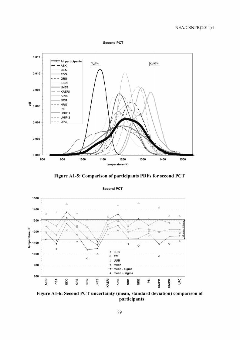
NEA/CSNI/R(2011)4
89
Second PCT
0.000
0.002
0.004
0.006
0.008
0.010
0.012
800 900 1000 1100 1200 1300 1400 1500
temperature (K)
All participantsAEKICEAEDOGRSIRSNJNESKAERIKINSNRI1NRI2PSIUNIPI1UNIPI2UPC
Yall5% Yall95%
Figure A1-5: Comparison of participants PDFs for second PCT
Second PCT
800
900
1000
1100
1200
1300
1400
1500
AEK
I
CEA
EDO
GR
S
IRSN
JNES
KA
ERI
KIN
S
NR
I1
NR
I2
PSI
UN
IPI1
UN
IPI2
UPC
tem
pera
ture
(K)
LUBRCUUBmeanmean - sigmamean + sigma
all:
mea
n ±
sigm
a
Figure A1-6: Second PCT uncertainty (mean, standard deviation) comparison of
participants

NEA/CSNI/R(2011)4
90
A1-3 Maximum PCT
The same work is done for the maximum PCT. The results are presented in Table A1-3 and Figures A1-7, -8 and -9.
7
Figure A1-7: Histogram and evaluated PDFs of all participants for maximum PCT
Summary of the distribution of all participants (Yall):
Mean value: allY = 1245 K Standard deviation: σYall = 75 K 5 % fractile: Yall5% = 1129 K 95 % fractile: Yall95% = 1367 K
Table A1-3: Maximum PCT uncertainty comparison by participant
LUB RC UUB Y
σY dd1 dd2 DKL P(i)
AEKI 1139 1216 1362 1251 56 0.1 0.0 0.2 0.04 CEA 1172 1252 1379 1250 51 0.1 0.0 0.6 0.03 EDO 1221 1326 1450 1326 48 0.9 0.7 3.0 0.19 GRS 1198 1293 1402 1299 55 0.6 0.4 0.9 0.11 IRSN 1142 1218 1392 1261 67 0.2 0.1 0.2 0.08 JNES 1089 1185 1238 1164 35 1.0 0.7 6.0 0.15 KAERI 1174 1247 1336 1264 42 0.2 0.2 0.8 0.01 KINS 1213 1291 1435 1305 51 0.7 0.5 2.0 0.12 NRI1 1090 1220 1304 1209 57 0.4 0.3 0.5 0.06 NRI2 1092 1221 1459 1230 87 0.1 0.1 0.2 0.16 PSI 1164 1206 1313 1222 35 0.3 0.2 1.5 0.00 UNIPI12 979 1198 1418 1199 110 0.3 0.3 0.2 0.31 UNIPI22 1093 1218 1342 1218 62 0.3 0.2 0.2 0.08 UPC 1119 1189 1342 1227 57 0.2 0.1 0.2 0.05 All 1245 75 0 0 0 0.10

NEA/CSNI/R(2011)4
91
As expected, the differences between participants are less pronounced for the maximum PCT than for the 1st or 2nd PCTs. The extreme values of the measures once again confirm what can be observed:
• EDO uncertainty band is located in the upper zone of all participants • The (narrow) JNES uncertainty band is located in the lower part of all participants.
However, this trend is less pronounced than for the 2nd PCT.
Maximum PCT
0.000
0.002
0.004
0.006
0.008
0.010
0.012
800 900 1000 1100 1200 1300 1400 1500temperature (K)
All participantsAEKICEAEDOGRSIRSNJNESKAERIKINSNRI1NRI2PSIUNIPI1UNIPI2UPC
Yall5% Yall95%
Figure A1-8: Comparison of participants PDFs for maximum PCT

NEA/CSNI/R(2011)4
92
Maximum PCT
900
1000
1100
1200
1300
1400
1500A
EKI
CEA
EDO
GR
S
IRSN
JNES
KA
ERI
KIN
S
NR
I1
NR
I2
PSI
UN
IPI1
UN
IPI2
UPC
tem
pera
ture
(K)
LUBRCUUBmeanmean - sigmamean + sigma
all:
mea
n ±
sigm
a
Figure A1-9: Maximum PCT uncertainty (mean, standard deviation) comparison of
participants
A1-4 Summary
Results of the uncertainty analysis of all participants of phase V of the BEMUSE programme are compared. Each participant provided the uncertainty results in terms of lower bound (LUB) and upper bound (UUB). The uncertainty bounds are extreme values by an estimation of the probability density function (pdf) or cumulative density function (cdf) describing these uncertainties. These distributions of calculated results are included in the comparison of this appendix. For technical reasons, only the single-valued output parameters are used. Among these output parameters, only the values of peak cladding temperature are treated, i.e. 1st PCT, 2nd PCT and the maximum PCT occuring in time and space. This information gives more insight into the results of different participants in a synthetic way.
NEA/CSNI/R(2011)4
93
APPENDIX 2: DESCRIPTION OF EVALUATION AND SYNTHESIS OF MULTIPLE SOURCES OF INFORMATION AND FURTHER APPLICATION TO AN ANALYSIS OF
BEMUSE PHASE III AND PHASE V COMPUTER CODE RESULTS
J. Baccou, E. Chojnacki, S. Destercke (IRSN, France)
Introduction
In order to come up with a comparison of uncertainty analyses performed in the frame of the BEMUSE Programme a new approach for comparing these results is presented here. When multiple sources provide information about the same set of variables, and when this information is tainted with uncertainty, it can be difficult to analyze and compare the different results obtained by each source. To complement the study achieved in two phases of BEMUSE, IRSN proposes, for BEMUSE phases III and V, to use formal methods coming from probability [A1] and possibility theory [A2] in order to analyze and compare the results of the uncertainty studies performed on the Zion reactor. Such methods usually consist in three steps:
• modelling the information provided by the sources
• evaluating the quality of the information from two criteria: informativeness and calibration
• synthesizing the information provided by the sources It should be kept in mind that this study is preliminary and that its main purposes are to show that such methods can be useful in the analysis of the information and to make some first conclusions about the benchmark. A full study would require a longer and deeper work, but interesting conclusions were already drawn from this preliminary study. All results provided have been computed by the means of SUNSET software
A2-1 Evaluation and synthesis methods
We now summarize how the tree steps (modelling, evaluation, synthesis) are done with the probabilistic and possibilistic approaches. Full details and ampler discussions can be found in related papers [A1], [A2], [A3]. In the following, we will consider that N sources s1,...,sN provide information about V different variables X1,...,XV

NEA/CSNI/R(2011)4
94
A2-1.1 Information representation
A2-1.1.1 Probabilistic approach
For each variable of interest, information provided by sources (experts, computer codes, captors) is modeled by a finite set of B+1 percentiles with the k% percentile denoted qk%. If the same B+1 percentiles are provided for each variable X1,...,XV , then the information on each variable can be modeled by an histogram or probability density p = (p1 , . . . , pB ) made of B interpercentiles. In the following, we will denote ql = q0% and qu = q100% the entire range of variation of one variable The figure below represents the cumulative distribution function (CDF) corresponding to the first peak cladding temperature of a reactor for which available information is q0% = 500 K, q5% = 600 K, q50% = 800 K, q95% = 900 K, q100% = 1000 K. The corresponding probability density p = (0.05, 0.45, 0.45, 0.05) is pictured in dashed lines.
A2-1.1.2 Possibilistic approach
A possibility distribution is formally a mapping π : R → [0, 1] from the reals to the unit interval. From this distribution, we can define two (conjugate) measures describing the likelihood of events: the possibility measure: Π(A) = AxSup ∈ π(x) the necessity measure: N (A) = 1 − Π(Ac ) with Ac the complement of A. To every value α ∈ [0, 1] we can associate an α-cut Aα which is the set A= {x|π(x) ≥ α}. When interpreted as a family of probability distributions [A4], a possibility distribution can be seen as a collection of nested intervals with lower confidence levels, that is P (Aα ) ≥ N (Aα ) (N (Aα ) = 1 − α), with P an imprecisely known probability.
A possibility degree of an event expresses the extent to which this event is plausible, i.e. consistent with our knowledge. Necessity degrees express the certainty of events.
A possibilistic distribution can also be interpreted as the simplest model describing a family of probability distributions [A4], and thus is a model of partial probabilistic information. Possibility distributions are candidates to model incomplete probabilistic information given in terms of confidence intervals, but can also be used when information concerns other characteristics, e.g. mean, percentiles, mode of the unknown probability distribution [A5].

NEA/CSNI/R(2011)4
95
The figure below represents a possibility distribution corresponding to the first peak cladding temperature of a reactor where information consists of four intervals [500 K, 1000 K], [600 K, 950 K], [650 K, 900 K], [750K, 850 K] which have respective confidence levels of 10%, 50%, 90% and 100%.
A2-1.2 Information evaluation
The information provided by the sources is evaluated by two different criteria, measuring different qualities: Informativeness: measure the precision of the information. The more precise is a source, the more useful it is. Calibration: measure the coherence between information provided by the source and the experimentally observed value (which can be observed after having received the source information). The probabilistic approach is performed globally, i.e. one calibration score taking into acount all output variables referred as “seed variables” PCT1, PCT2, injection and quench time. In the possibilistic approach the scores are calculated individually, i.e. one calibration score for each of the four output variables which are then averaged to derive the value provided in Table A2-1, for example.
A2-1.2.1 Probabilistic approach
Informativeness: let p = (p1 , . . . , pB ) be the probability density modeling the source information for a variable X, and u = (u1 , . . . , uB ) be the uniform density for the same variable on the same range of variation (u = (0.20, 0.40, 0.20, 0.20) for the example given above). The informativeness I(p,u) for this source on variable X is simply the relative entropy
∑=
=
B
i i
ii u
ppupI1
log),(
and if the source gives information on V variables, the global informativeness is simply the mean of informativeness scores over all these variables. Calibration: given a set of V variables X1,...,XV for which the source have given information and for which we have experimental values, calibration scores assume that, for a perfectly calibrated source, p1% of the true values will fall in interpercentile 1, p2% in interpercentile 2, ... Now, if in reality r1V values fall in interpercentile 1, r2V in interprecentile 2, we can build an empirical distribution p = (p1 , . . . , pB ), and compute the divergence of p from r. (i.e., the surprise of learning r when p is thought to be the right answer)

NEA/CSNI/R(2011)4
96
∑=
=
B
i i
ii p
rrprI1
log),(
which is minimal (=0) if and only if r=p. As it is known that 2*N*I(r,p) tends to a chi-square distribution with B-1 degree of freedom (N being the number of observed values), the final value of the calibration for a given source s is
( )),(**21)( 12 prINsCal Bp −−= χ
The construction of distributions r is illustrated below, where the common interpercentile distribution is p = (0.05, 0.45, 0.45, 0.05) since each source provides the q0%, q5%, q50%, q95% and q100% percentiles. The empirical distribution for the source 1 is r1 = (0, 0.5, 0.5, 0), because the realization of the variable 1 falls in the 2nd interpercentile and the realization of the variable 2 falls in the 3rd interpercentile. In the same way, the empirical distribution for the source 2 is r2 = (0.5, 0, 0.5, 0), because the realization of the variable 1 falls in the 1st interpercentile and the realization of the variable 2 falls in the 3rd interpercentile.
The final score is then obtained as the product of both calibration and informativeness (the product which is used as a good source has to be informative and well calibrated)
A2-1.2.2 Possibilistic approach
Informativeness: let πs be the distribution modeling source s information for one variable and πign the distribution corresponding to interval [ql,qu] ( πign(x)=1 if x ∈ [ql,qu], zero otherwise). Then, the informativeness of source s is simply
ign
signsIπ
πππ
−=),(
with |πs| the cardinality of πs which reads ∫=u
l
q
qs dxx)(ππ . This is simply the area under the distribution. If
a source provides information for multiple variables, the final informativeness is simply the average of all informativeness over all variables.

NEA/CSNI/R(2011)4
97
Calibration: assume the (true) value x* of a variable is observed experimentally. Then, the calibration of source s is simply the value πs(x*), that is how much the value x* is judged plausible by the information given by the source. If information is given for multiple variables, the final calibration score is again the average of all calibration scores. Note that, in the case of possibilistic approach, calibration is computed individually for each variable (whereas it was done globally in the probabilistic approach)
A2-1.3 Information synthesis
Synthesizing the information allows to build a summary of all information provided by the sources, and also to make further analysis. Among other things, it allows to quantify the potential conflict between information given by different sources. It is common to distinguish three main kinds of synthesis behaviors:
• conjunctive: equivalent to take the intersection, conjunctive synthesis assumes the reliability of all sources, and allows to quantify the conflict among sources. It produces precise but potentially unreliable results in case of strong conflict,
• disjunctive: equivalent to take the union, disjunctive synthesis makes the conservative assumption that at least one source is reliable. It produces in general imprecise but reliable results,
• arithmetic (weighted) mean: assumes independence between sources, and produces a result between disjunction and conjunction.
A2-1.3.1 Probabilistic approach
It is now commonly accepted among researchers [A1] of the field that the arithmetic weighted is the best approach to synthesis probability distributions. Also, there is no real counterpart to set intersections and unions in the probability field, therefore conjunction and disjunction are difficult to formally define. If N sources give their opinion in the form of distributions p1,...,pN, and if to each distribution is associated a weight wi (e.g., computed via previous methods) such that their sum is one, the arithmetic weighted mean reads
∑=
=N
iiimean pwp
1
and the result is illustrated by the figure below

NEA/CSNI/R(2011)4
98
A2-1.3.2 Possibilistic approach
For the possibilistic approach, the three kinds of operators [A4] are well defined. If π1,..., πN are the distributions provided by the N sources, then they read:
• conjunction: π∩(x) = mini =1,...,N (πi (x)) • disjunction: π ∪ (x) = maxi =1,...,N (πi (x))
• arithmetic mean: πmean (x) = ∑=
N
i 1
(πi (x))
These three behaviors are summarized in the figure below when two sources provide information.
Note, that in the case of conjunction of multiple sources, the height h between the result and the value 1 quantify the conflict among a subgroup of sources.
A2-2 Application to the analysis of BEMUSE phase III results
The organisation IRSN evaluated the results of phase III using the new method of evaluation and synthesis of multiple sources of information. The results of that evaluation are presented in the following sections.
A2-2.1 Considered variables
In a first step, IRSN has limited its study of BEMUSE phase III results to the four scalar parameters evaluated in the 3 first phases, that is: the first peak cladding temperature (1PCT), the second peak cladding temperature (2PCT), the injection time (tinj) and the complete quench time (tq). The information kept for each of these variables was the lower and upper confidence bounds provided by each participants, as well as the reference value (taking account of all calculations does not change the main conclusions of the analysis, and only add unnecessary complexity). Actually, taking account of time dependent variables would be desirable in a deeper study, but limiting oneself to scalar variables is satisfactory in a first study. In Table A2-1 the values provided by each participant are summarized, as well as the experimental values obtained.

NEA/CSNI/R(2011)4
99
Table A2-1: Calculated uncertainty ranges by different participants compared with
measured values for the single-valued results
A2-2.1.1 Modeling of the information
In a probabilistic approach information is provided by a finite set of percentiles or a probability density for each variable of interest.
A possibility degree of an event expresses the extent to which this event is plausible, i.e. consistent with our knowledge. A possibilistic distribution can also be interpreted as the simplest model describing a family of probability distributions [A4], and thus is a model of partial probabilistic information. Possibility distributions are candidates to model incomplete probabilistic information given in terms of confidence intervals, but can also be used when information concerns other characteristics, e.g. mean, percentiles, mode of the unknown probability distribution [A5].
The first step was to model the information provided by each participant (source). First, for each variable, the entire variation domain [ql,qu] was chosen to be 102% of the entire variation between the minimal and maximal values given by all participants (e.g., for 1PCT, min = 626 (KINS), max = 1255 (CEA) and [ql,qu] = [620,1261]). Probabilistic modelling: For each participant and variable, we take their lower and upper limit as respectively the percentiles 1% and 99%. The percentiles q0% andq100% correspond to ql and qu defined in the former paragraph. For example, for NRI1 and the 2PCT, we have q0% = 592, q1% = 845, q50% = 1012, q99% = 1167, q100% = 1228.

NEA/CSNI/R(2011)4
100
Possibilistic modelling: concerning the possibilistic model of the information, the reference value can be interpreted as the most plausible, thus receiving a possibility degree of 1. According to our previous remark, the interval [Low, Up] is similar to an interval with a lower confidence of 98% (and the two values receive a possibilistic degree of 0.02). The next Figure A2-1 shows the model corresponding to the information given by NRI1 for the 2PCT for both modellings, possibilistic and probabilistic. The figure shows the triangular possibility distribution at the top. At the bottom is the CDF of the histogram density distribution (q0% = 592, q1% = 845, q50% = 1012, q99% = 1167, q100% = 1228) in the probabilistic framework.
0
0,1
0,2
0,3
0,4
0,5
0,6
0,7
0,8
0,9
1
592 692 792 892 992 1092 1192T (K)
0
0,0005
0,001
0,0015
0,002
0,0025
0,003
0,0035
592 692 792 892 992 1092 1192
T (K)
Figure A2-1: Possibility (top) and probability distributions (bottom) of NRI1 for the 2nd PCT

NEA/CSNI/R(2011)4
101
A2-2.1.2 Evaluation
As we have available, for each variable, an experimental value, it is possible to evaluate the quality of the information delivered by each source. Table A2-2 summarizes the results obtained for the four considered single-valued variables. Indicated are the ranks for each participant and each criterion, as well as the exactly computed values in parenthesis. The evaluation was performed according to the method described in the Appendix. Table A2-2 summarizes the obtained informativeness, calibration and global scores for informativeness and calibration. Informativeness measures the precision of the information, i.e. a narrow uncertainty range gives high precision. Calibration expresses how well the calculated results of a participant agree with experimental values. Global scores for informativeness and calibration take into account both criteria; the values in brackets for informativeness and calibration are multiplied. The global score is a compromise between narrow uncertainty range (informativeness) and agreement with experimental values (calibration).
Table A2-2: Informativeness, calibration and global scores for probabilistic and possibilistic approach, lowest numbers (highest values in brackets) express the highest score
Table A2-3 summarizes the ranking of participants based on that evaluation for the four considered variables within both probabilistic and possibilistic frameworks.

NEA/CSNI/R(2011)4
102
Table A2-3: Ranking of participants of the LOFT comparison
Rank Probabilistic approach Possibilistic approach 1 GRS IRSN 2 IRSN NRI2 3 NRI1 KINS 4 UNIPI NRI1 These results are to be taken with caution, for reasons that should be kept in mind:
• Limited number of variable: Instability in the results and poor discriminative power (e.g., similar calibration scores for the probabilistic approach) are due to the relatively poor quantity of variables considered.
• Primary study: This is a primary study and an illustration of how new tools coming from uncertainty theories can help in the analysis of information.
• Results as an analysis tool: Although the primary aim of these tools is to assess sources reliability, they are here used as analysis tools, and should not be perceived as absolute judgment. Using them as formal validation tool would effectively require a more careful thinking about what has to be validated.
But, even if those results can be criticized, we can still draw some useful conclusions from them:
• User effect on results: From above table, it can be seen that users of the same code (KINS, NRI1, UPC, UNIPI for RELAP5, CEA and IRSN for CATHARE, GRS and NRI2 for ATHLET) can have very different scores. This indicates that the user expertise, as well as how uncertainties are modelled, play important roles in the quality of the final result.
• Uncertainty underestimation: Both PSI and UPC have received very good informativeness scores with bad calibration scores. This indicates that they probably both tend to underestimate the uncertainties in the input parameters. The experimental values are close to the upper bound or even outside the calculated range.
• The experimental value is always within the GRS uncertainty band, once out of the KINS band and twice out of the PSI and UPC bands.
• Uncertainty overestimation: In both approaches, UNIPI has the worst informativeness score, while having a good calibration score. This indicates that, compared to other participants, its method has a tendency to overestimate final uncertainties, while guaranteeing a good accuracy.
As said before, these results can also be helpful to validate computer codes (e.g., by fixing minimal required values for accuracy and informativeness).
A2-2.1.3 Synthesis
Figure A2-2 below show the result of aggregating the probability distributions modelling the information of the different participants for the second peak cladding temperature (2PCT), first by codes, then by using the weights computed in the evaluation step directly in the arithmetic mean to select subgroup of sources.

NEA/CSNI/R(2011)4
103
Figure A2-2: Application of probabilistic aggregation for the 2nd PCT The left figure shows and allows detecting that results grouped by used code have either a tendency to provide an underestimation (RELAP5, CATHARE) or an overestimation of the true value (ATHLET). Whether this tendency is systematic and due to the specific used code would be matter of further investigation. The right figure indicates that taking into account weights and subgroup of sources (here, the first four sources given by the probabilistic method and the four sources common to the first five sources given by each method) is helpful to improve the final result. We see that considering only the sources considered as the best by both approaches and their associated weights provides a narrower (better informativeness) distribution that is more centred around the experimental value (better calibration). Figures A2-3 and 4 summarize the results obtained by applying the classical arithmetic weighted mean, disjunction and conjunction (again first by selecting sources using a specific code and then by selecting subgroups of best sources).

NEA/CSNI/R(2011)4
104
Figure A2-3: Application of possibilistic aggregation for the 2nd PCT: Disjunction (left) and weighted mean (right)
Figure A2-4: Application of possibilistic aggregation: Conjunction (minimum) for the 2nd PCT
We see here that the disjunction is very imprecise, but also very reliable (experimental value is in the interval with lower confidence 20% only). We can also see that most sources tend to underestimate the true, i.e. experimental value (as most peaks are lower than this value). Again, verifying that this bias is systematic requires further investigation. The arithmetic weighted mean do not bring much information, and has, as in the probabilistic case, a “smoothing” effect. Nevertheless we can see that the resulting distribution has a relatively good calibration and informativeness, i.e. is a good compromise. The conjunctive behaviour is the most interesting, since it tells us that the conflict between results obtained by CATHARE users is lower (higher values of π(x)) than the one obtained for ATHLET users. This could come from the fact that ATHLET users have more uncertain input parameters than CATHARE users (49
NEA/CSNI/R(2011)4
105
and 64 versus 42 and 52). The higher conflict for RELAP5 users can be explained by the fact that more participants were using this particular code.
The distribution resulting from the conjunction of ATHLET users is very precise and exhibits a peak very close to the experimental value. Since the experimental value of the 2nd peak cladding temperature is known, this distribution is preferred against the others in Figure A2-4. Otherwise, one would have given low credit to that distribution due to its relatively low reliability which comes from the larger reference value by GRS and the lower one by NRI2 compared with the experimental value. We also see that, by selecting only subgroups of sources that had good ranking in the evaluation procedure, we obtain a result that is highly coherent (i.e., with a low conflict), and can therefore be judged as reliable. The fact that the best sources are coherent between them also increases our confidence in the obtained result. Conjunction also indicates that there is a strong conflict if we take all sources into account. This information is potentially useful, as we have now identified a conflict, which causes can be investigated.
A2-2.1.4 Conclusions on the evaluation of phase III results
This first study has shown how new techniques coming from uncertainty theories can help in the analysis and the evaluation of information coming from multiple sources (computer codes, experts, data bases, etc.).
These techniques allows, among other things, to provide more information than classical metrics like distances, and in this sense complements their conclusions. They offer formal frameworks that permit to reach new conclusions (quantification of informativeness/calibration, conflicts identification) or to formally confirm informal knowledge.
In practice, a careful study using such techniques, in collaboration with experts, can help to identify some problems and to search more efficiently for their causes. That may help organisations to improve their tools. Moreover, the approaches used can serve as generic tools to address old problems with new views, such as the challenge of formal code validation.
A2-3 Application to the analysis of BEMUSE phase V results
This section is devoted to the application of the previous tools in order to analyse the information provided by each participant during BEMUSE phase V.
A2-3.1 Considered variables
We have limited this study to the five scalar parameters: First Peak Cladding Temperature (PCT1), Second Peak Cladding Temperature (PCT2), Accumulator Injection Time (TInj), Complete Core Quench Time (Tq) and Maximum Cladding Temperature (MaxCladT). Taking account of time dependent variables would be desirable in a deeper study, but limiting oneself to scalar variables is satisfactory in a first study. The information kept for each of these variables was the lower and upper confidence bounds provided by each participant, as well as the reference value (see Tables 13-17 of the BEMUSE phase V report [A6]). Since KAERI did not obtain complete core quenching in the upper bound case, this institute is not considered in the analysis of the results related to Tq.
A2-3.2 Modelling
The first step was to model the information provided by each source. First, for each variable, the entire

NEA/CSNI/R(2011)4
106
variation domain [ql,qu] was chosen to be 102% of the entire variation between the minimal and maximal values given by all participants (e.g., for PCT1, min = 792 K (UNIPI2), max = 1393 K (GRS) and [ql,qu] = [786 K,1399 K]). probabilistic modeling: Except for UNIPI1 and UNIPI2, all the participants obtained the lower and upper bound values so that they were respectively lower and larger than the 5% and 95% percentiles with 95% confidence level (according to order statistics, often quoted as Wilk’s formula). These lower and upper bounds can be considered as conservative evaluations of the 5% and 95% percentiles of the unknown probability distributions. Therefore, it seems natural to take them as best estimates of, respectively, the 1% and 99% percentiles. With the notations of Tables 13-17 of BEMUSE Phase V report [A6], we take for each participant and variable (q0%, q1%, q50%, q99%, q100%) = (ql, LUB, RC, UUB, qu) as a probabilistic model. For example, for NRI1 and PCT1, we have q0% = 786 K, q1% = 1046 K, q50% = 1191 K, q99% = 1299 K, q100% = 1399 K. possibilistic modeling: concerning the possibilistic model of the information, the reference calculation can be interpreted as the most plausible, thus receiving a possibility degree of 1. According to our previous remark, the interval [LUB,UUB] is similar to an interval with a lower confidence of 98% (and the two values receive a possibilistic degree of 0.02).
A2-3.3 Source evaluation
Source evaluation (informativeness and calibration) allows us to evaluate the quality of the information delivered by each source. It is possible provided we possess, for each variable, an experimental value, which is not the case in BEMUSE phase V. However, this evaluation has been performed for PCT1, PCT2, TIng and Tq in a previous study in the frame of BEMUSE phase III (LOFT L-2-5 experiment). It has led to a ranking of participants according to each criterion (calibration and informativeness) and to their global score. It seems to be relevant to integrate these results in the analysis of the Zion results in order to check if the information provided by the “high ranked” participants of the LOFT benchmark (identified as reliable sources) is still in agreement for this new benchmark. The table below was already presented in the evaluation of phase III, and is repeated here to summarize the ranking obtained for the four considered variables within both probabilistic and possibilistic frameworks.
Table A3-1: Ranking of participants of the LOFT benchmark Rank Probabilistic approach Possibilistic approach 1 GRS IRSN 2 IRSN NRI2 3 NRI1 KINS 4 UNIPI1 NRI1 These results, obtained in a previous study, are to be taken with caution, for reasons that should be kept in mind:
• limited number of variables: as the previous evaluation for the small-scale facility has been done for only a few variables (4), there was some instability in the results.
• primary study: this is a primary study and an illustration of how new tools coming from uncertainty theories can help in the analysis of information and in particular, in the present study, how previous evaluations can help in those cases where the true value is unknown .
• results as an analysis tool: although the primary aim of these tools are to assess sources reliability, they are here used as analysis tools, and should not be perceived as absolute judgment. Using them

NEA/CSNI/R(2011)4
107
as formal validation tool would effectively require a more careful thinking about what has to be validated.
• Only 10 participants have been involved in the LOFT benchmark. Therefore, the source evaluation does not integrate any information delivered by EDO, UNIPI2, JNES and AEKI. This is why we cannot directly use here weights computed within the LOFT benchmark in some weighted aggregation procedures.
A2-3.4 Information synthesis
We first propose a synthesis of the whole information given by participants with a special attention devoted to subgroups of participants that are in agreement in their results. Then, we study the influence of the used code and of the uncertainty methods on the derivation of uncertainty margins.
A2-3.4.1 Synthesis of the information given by all participants
We provide in the sequel the information summary that can be extracted for each variable within probabilistic and possibilistic frameworks.

NEA/CSNI/R(2011)4
108
Figure A2-5: Mean aggregation within the probabilistic framework
Figure A2-5: Mean aggregation within the probabilistic framework
Probabilistic aggregation: Figure A2-5 displays the results of aggregating the probability distributions of the various participants. Each arithmetic mean is used with equal weights. We have also plotted the probability distributions coming from the aggregation associated to the four “high ranked” participants (Table A2-3).
0
0,1
0,2
0,3
0,4
0,5
0,6
0,7
0,8
0,9
1
800 900 1000 1100 1200 1300 1400 1500 1600
F
Max Clad T

NEA/CSNI/R(2011)4
109
Table A2-4 summarizes the information related to the uncertainty margins. The lower (resp. upper) uncertainty bound is the 5% (resp. 95%) - percentile of each previous probability distribution. The reference (Best-estimate) calculation is identified to the 50%-percentile.
Table A2-4: Uncertainty margins coming from the aggregated information (for all participants)
Note that the probability distributions provided by the four “high ranked” participant aggregation is close to the distribution aggregated from all participants. In the case of TInj, it provides narrower uncertainty margins. This illustrates that, in some cases, using the ranking of the LOFT benchmark can be useful to increase the precision of the information. However, a potential conflict between participants is hardly visible. Moreover, the arithmetic mean tends to average the resulting distribution, which could explain that the two distributions remain close although different. For a deeper analysis of this benchmark, the possibilistic aggregation is considered in the sequel. Possibilistic aggregation: a) Mean aggregation: Figure A2-6 shows the result of applying the usual compromise operator (i.e. equal weighted arithmetic mean) of all participants. Except for TInj, the arithmetic mean averages the contribution of all participants leading to a smooth distribution. As for the accumulator injection time, the aggregated distribution exhibits several peaks that are due to the narrow uncertainty margin given by each participant and a dispersion of the reference calculation (Std Dev(RC) = 3.1) which is close to the average uncertainty band width (Mean(UUB-LUB)=4.1) and even bigger (Mean(UUB-LUB)=1.1) if we don’t consider UNIPI1 and UNIPI2 that have given very large uncertainty bands compared to the other participants. The participants are expected to be highly conflicted in that case, which will be confirmed by the conjunctive aggregation in Section c).
5%-percentile BE 95%-percentile PCT1 (K) 1002.8 1210.8 1354.9 PCT2 (K) 1019.7 1221.2 1400.1 Tinj (s) 11.2 14.8 23.2 Tq (s) 133.8 243.6 484.7 MaxCladT (K) 1072.5 1238.7 1396.1

NEA/CSNI/R(2011)4
110
Figure A2-6: Mean aggregation within the possibilistic framework Following this previous remark and for sake of comparison with the probabilistic aggregation, Table A2-5 provides, for PCT1, PCT2, Tq and MaxCaldT, the “Best Estimate” (resp. “the set of Best Estimates”) corresponding to the value (resp. the interval) associated to the highest possibility degree of each distribution. We have also added in the last column the average conflict which allows us to measure if participants’ results are similar in mean.
PCT1
0
0,1
0,2
0,3
0,4
0,5
0,6
0,7
0,8
0,9
1
750 850 950 1050 1150 1250 1350 1450PCT1(K)
π All participan
PCT2
0
0,1
0,2
0,3
0,4
0,5
0,6
0,7
0,8
0,9
1
820 920 1020 1120 1220 1320 1420PCT2(K)
π All participants
TInj
0
0,1
0,2
0,3
0,4
0,5
0,6
0,7
0,8
0,9
1
4,5 9,5 14,5 19,5 24,5 29,5Tinj(S)
π All participan
Tq
0
0,1
0,2
0,3
0,4
0,5
0,6
0,7
0,8
0,9
1
100 200 300 400 500 600 700Tq(S)
π All participants
MaxCladT
0
0,1
0,2
0,3
0,4
0,5
0,6
0,7
0,8
0,9
1
800 900 1000 1100 1200 1300 1400 1500 1600MaxCladT(K)
π All particpan

NEA/CSNI/R(2011)4
111
Table A2-5: “Best Estimate(s)” coming from the possibilistic mean aggregation
It turns out that, for each output of interest with a low average conflict (i.e < 0.5), the result coming from the possibilistic approach encompasses (is close to) the “Best Estimate(s)” associated to the probabilistic approach. b) Disjunctive aggregation Figure A2-7 displays the distributions after applying the disjunctive operator to all participants. As expected, the result is quite imprecise since it is performed by combining the uncertainty margins of all participants. However, Figure A2-7 exhibits very interesting information for the analysis:
• UNIPI1 calculated the lowest PCT1 reference value compared with other participants. Moreover, the majority of reference calculations are closer to the upper bound of the support of the distribution than to the lower bound. This is due to the lower bound of the uncertainty margin given by UNIPI2 that is rather small compared to the lower bound of participants using a probabilistic approach. On the contrary, the upper bound of the distribution support is fixed by the upper bound of the GRS uncertainty margin which corresponds to a “reasonable” upper bound for probabilistic users. For the same reason, a “dissymmetry” in the distribution appears in the cases of PCT2 and MaxCladT. Therefore, splitting the analysis with respect to the uncertainty methodology (CIAU/Probabilistic) appears to be necessary for a better understanding of this benchmark. It can help in increasing the informativeness of the aggregated distribution (compare for PCT1, [1054K; 1306K] for the highest possibility degree with UNIPI1 and [1178K; 1306K] without UNIPI1) while analysing in deep the difference between methodologies.
• Concerning Tq, the lowest value (136.1s, EDO) associated to the highest degree of possibility is close to the lower bound of the support of the distribution. This shows that some participants have provided a reference calculation close to the lower bound of their corresponding uncertainty margin and that this lower bound is among the lowest uncertainty bounds of all participants. This is the case for example for EDO with RC-LUB=12s, UUB-RC=243.2s and LUB=124.1s.
• Note also that the distribution associated to TInj is in full agreement with the results coming from the distribution after arithmetic mean aggregation. The disjunctive operator leads to a distribution with several peaks indicating a large dispersion of reference calculations provided by all participants combined with a narrow uncertainty band width.
Possibilistic app. Probabilistic app. Average conflict PCT1 (K) [1187;1218] 1210.8 0.4 PCT2 (K) 1220 1221.2 0.34 Tq (s) 205 243.6 0.55 MaxCladT (K) [1213;1252] 1238.7 0.45

NEA/CSNI/R(2011)4
112
Figure A2-7: Disjunctive aggregation within the possibilistic framework

NEA/CSNI/R(2011)4
113
Table A2-6: Subgroups of participants with a close reference calculation
For every output of interest but Tq, one can exhibit subgroups of participants that have provided close reference calculations and therefore, that are expected to be in agreement in their analysis. They are listed in table A2-6. The coherence of each subgroup will be tested by applying the conjunctive aggregation. c) Conjunctive aggregation Figure A2-8 displays the distributions after applying the conjunctive operator to all participants, to the selected participants of the LOFT benchmark and to the subgroups of participants summarized in Table A2-6.
Output variables Subgroups of participants
PCT1 AEKI, IRSN, JNES, KAERI, NRI1, NRI2, PSI, UNIPI2, UPC
PCT2 AEKI, NRI1, NRI2, PSI, UNIPI1, UNIPI2, UPC
TInj AEKI, IRSN, KINS, NRI1, UNIPI1, UNIPI2, UPC
MaxCladT IRSN, JNES, NRI1, NRI2, PSI, UNIPI1, UNIPI2, UPC
0,1
0,2
0,3
0,4
0,5
0,6
0,7
0,8
0,9
1
π
0
0,1
0,2
0,3
0,4
0,5
0,6
0,7
0,8
0,9
1
800 900 1000 1100 1200 1300 1400 1500 1600
π
PCT2(K)
PCT2
All par ticipa nts
"Be st" p art icipan ts
AEKI, NRI1, NRI2, PSI, UNI PI 1,UNIPI2, UPC

NEA/CSNI/R(2011)4
114
Figure A2-8: Conjunctive aggregation within the possibilistic framework
Let us first notice that all the participants are highly conflicting for each output variable, which reduces the reliability of the information synthesised from all of them. The conflict is reduced for PCT1, PCT2 and MaxCladT when considering the selected four participants. However, it remains quite high, especially for PCT2, indicating that the ranking obtained for the LOFT experiment has to be taken with caution for result prediction within the Zion case. Note also that the selected four participants and the subgroups of participants of Table A2-6 provide similar results for PCT1, PCT2 and MaxCladT. The closest estimation (best estimate and uncertainty margins) given by the two subgroups is related to PCT2. That tends to confirm the reliability of the information coming from these sources about this variable, keeping in mind that due to lost of coherence of the selected participants between LOFT and ZION exercises, this result has to be taken with caution. As for MaxCladT, even if the information given by the four selected participants and by the subgroups of Table A2-6 is coherent, it is not straightforward to take into account their information since their conjunctive aggregation is highly conflicting (intersection almost empty). Concerning TInj, focussing on the subgroup of Table A2-6 increases the reliability of the information related to this variable. The result is very precise (due to narrow uncertainty margin) with a low degree of conflict (~0.4). For Tq, considering the four selected participants does not increase the coherence of the synthesized information. This can be explained by the underestimation of the upper uncertainty bound by
Tinj
0
0,1
0,2
0,3
0,4
0,5
0,6
0,7
0,8
0,9
1
4 9 14 19 24 29
Tinj(S)
π
All participants"Best" participantsAEKI, IRSN, KINS, NRI1, UNIPI1, UNIPI2, UPC
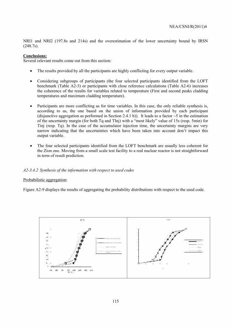
NEA/CSNI/R(2011)4
115
NRI1 and NRI2 (197.8s and 214s) and the overestimation of the lower uncertainty bound by IRSN (248.7s). Conclusions: Several relevant results come out from this section:
• The results provided by all the participants are highly conflicting for every output variable.
• Considering subgroups of participants (the four selected participants identified from the LOFT benchmark (Table A2-3) or participants with close reference calculations (Table A2-6) increases the coherence of the results for variables related to temperature (First and second peaks cladding temperatures and maximum cladding temperature).
• Participants are more conflicting as for time variables. In this case, the only reliable synthesis is, according to us, the one based on the union of information provided by each participant (disjunctive aggregation as performed in Section 2.4.1 b)). It leads to a factor ~5 in the estimation of the uncertainty margin (for both Tq and TInj) with a “most likely” value of 15s (resp. 5min) for Tinj (resp. Tq). In the case of the accumulator injection time, the uncertainty margins are very narrow indicating that the uncertainties which have been taken into account don’t impact this output variable.
• The four selected participants identified from the LOFT benchmark are usually less coherent for the Zion one. Moving from a small scale test facility to a real nuclear reactor is not straightforward in term of result prediction.
A2-3.4.2 Synthesis of the information with respect to used codes
Probabilistic aggregation: Figure A2-9 displays the results of aggregating the probability distributions with respect to the used code.

NEA/CSNI/R(2011)4
116
Figure A2-9: Mean aggregation within the probabilistic framework (Effect of used code)
The distributions are very different from one code to another, especially for Tq where a large gap between CATHARE users and TRACE/ATHLET/RELAP5 users is noticeable. This points out that the used code effect is not negligible. In the case of TInj, the distribution exhibits a strong change in its behavior between 15s and 20s for ATHLET users. It translates the large gap between the uncertainty margins of AEKI/GRS (~[13.8s;15.1s]) and of NRI2 ([19.6s;20.5s]).
Table A2-7 summarizes the best estimate value (or 50%-percentile) for each code and each output variable and its comparison to the mean value listed in Tables 13-17 of BEMUSE phase V report [A6]. We also find relevant to provide for each output variable which code gives the narrowest and the largest uncertain margins, denoted NUM and LUM.

NEA/CSNI/R(2011)4
117
Table A2-7: Used code effect: best estimates, comparison to Mean value (“+”, resp. “-”, is for “bigger”, resp. “smaller”, than the mean value) and code name leading to the narrowest and to the
largest uncertainty band
Output Variable
Best estimate Best estimate/Mean NUM LUM TRACE RELAP5 CATHARE ATHLET TRACE RELAP5 CATHARE ATHLET
PCT1(K) 1181 1183 1231.2 1242.2 - - + + TRACE CATHARE PCT2(K) 1147.1 1237 1163.7 1229.5 - + - + TRACE RELAP5 TInj(s) 12.5 15.2 14.4 15.2 - - - - TRACE CATHARE Tq(s) 250.4 195.3 364.1 214.8 - - + - RELAP5 CATHARE MaxCladT(K)
1196.7 1237 1234.1 1272.5 - + - + TRACE RELAP5
Note that TRACE users always obtained a best-estimate value lower than the mean. They provide also the narrowest uncertainty margin except for Tq while CATHARE users get the largest band for a majority of output variables. Possibilistic aggregation: Figure A2-10 displays the distributions after applying the conjunctive operator with respect to the used code.

NEA/CSNI/R(2011)4
118
Figure A2-10: Conjunctive aggregation within the possibilistic framework (Effect of used code)
The previous figure gives a way to measure the coherence between users of a same code by evaluating the degree of conflict for each distribution. In Table A2-8, we have ranked the codes according to their coherence between users, specifying each time the corresponding degree of conflict. The conflict is calculated as the difference between one and the highest value of possibility common to the usesrs of the same code.
Table A2-8: Coherence between users of a same code Output variable ATHLET CATHARE TRACE RELAP5 PCT1 3 (~0.35) 2 (~0.2) 1 (~0.04) 4 (~1) PCT2 1 (~0.13) 2 (~0.2) 4 (~1) 3 (~0.45) TInj 4 (~1) 4 (~1) 4 (~1) 1 (~0.4) Tq 2 (~0.7) 1 (~0.4) 4 (~0.79) 3 (~0.78) MaxCladT 3 (~0.4) 1 (~0.17) 2 (~0.22) 4 (~0.45)
For PCT1, PCT2 and MaxCladT, and for a large majority of codes, the results are coherent and therefore can be considered as reliable information. In the case of PCT1, the very low degree conflict of TRACE users can be due to the small number of users (2). On the contrary, the high conflict of RELAP5 users can be explained by the disjoint uncertainty margins of KINS and UNIPI1 ([1178K, 1375K] and [906K, 1176K] respectively). The degree of conflict is reduced to 0.3 (not shown in this report) if we remove UNIPI1 from the RELAP5 users. This result again emphasizes that the impact of uncertainty methodologies (CIAU/probabilistic) is not negligible in this study. Note also that TRACE has a high degree of conflict for PCT2. This is due to disjoint uncertainty margins. As for TInj and Tq, few users are coherent. In the case of TInj, the only coherent information has been given by RELAP5 users and the corresponding information is very precise. The other sources have an empty intersection. This can be explained by the dispersion of reference calculations among users of a same code (for example 14.9-12.9=2s for CATHARE IRSN and CEA users) and a narrow uncertainty band (1.2s). We have also computed from Table A2-8 the average degree of conflict for each code. It turns out that CATHARE users have the lowest degree of conflict (~0.4) whereas TRACE users the highest (~0.6, same score as for RELAP5 but with only two participants). This is directly connected to the large (resp. narrow) uncertainty band width provided by CATHARE users (resp. TRACE users).

NEA/CSNI/R(2011)4
119
Conclusions: Several relevant results come out from this section:
• Code effect is not negligible in the derivation of uncertainty margins.
• For a large majority of codes, users are coherent when estimating uncertainty related to the first and second peak cladding temperatures and to the maximum cladding temperature. Concerning scalar variables, only one code among four exhibits a low degree of conflict. This arises again the question of reliability in the prediction of accumulator injection time and complete core quench time.
• TRACE users tend to provide reference calculations lower than the mean value of all code users and the narrowest uncertainty margins. On the contrary, CATHARE users get the largest uncertainty band width for most of the variables of interest.
A2-3.4.3 Synthesis of the information with respect to uncertainty method
Probabilistic aggregation: Figure A2-11 displays the results of aggregating the probability distributions for CIAU and probabilistic users separately.
0 1
0,2
0,3
0,4
0,5
0,6
0,7
0,8
0,9
1
F
PCT1
P
CU
0
0,1
0,2
0,3
0,4
0,5
0,6
0,7
0,8
0,9
1
700 800 900 1000 1100 1200 1300 1400 1500 1600
F
PCT2(K)
PCT2
Probabilistic
CIAU
0
0,1
0,2
0,3
0,4
0,5
0,6
0,7
0,8
0,9
1
0 5 10 15 20 25 30
F
Tinj(S)
Tinj
PC
0
0,1
0,2
0,3
0,4
0,5
0,6
0,7
0,8
0,9
1
0 100 200 300 400 500 600 700
F
Tq(S)
Tq
ProbabilisticCIAU

NEA/CSNI/R(2011)4
120
Figure A2-11: Mean aggregation within the probabilistic framework (Effect of uncertainty method)
Table A2-9 summarizes the information related to uncertainty margins:
Table A2-9: Uncertainty method effect: best estimates and uncertainty band width for CIAU and probabilistic methods
Output variable CIAU Probabilistic
BE 95% percentile-5% percentile
BE 95% percentile-5% percentile
PCT1(K) 1088.3 486 1218 262.3 PCT2(K) 1207.9 481.2 1222.7 364.8 TInj(s) 15.6 19.4 14.8 11.5 Tq(s) 293.4 218.2 229.5 369.2 MaxCladT(K) 1207.9 481.1 1242.2 277.1 For output variables related to temperature (PCT1, PCT2 and MaxCladT), CIAU method leads to a best estimate smaller than in the probabilistic case. It is the contrary for the output variables related to time (TInj and Tq). Except for Tq, CIAU method provides larger uncertainty bands due to a different way of estimating uncertainty margins.
Possibilistic aggregation: Figure A2-12 displays the distributions after applying the conjunctive operator. We have also plotted the results provided by the probabilistic users of the subgroups of Table A2-6.
0
0,1
0,2
0,3
0,4
0,5
0,6
0,7
0,8
0,9
1
700 800 900 1000 1100 1200 1300 1400 1500 1600
F
MaxCladT
Pro
CIA
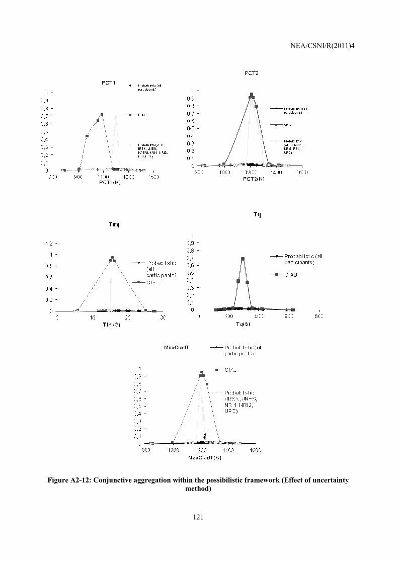
NEA/CSNI/R(2011)4
121
Figure A2-12: Conjunctive aggregation within the possibilistic framework (Effect of uncertainty
method)

NEA/CSNI/R(2011)4
122
It appears that CIAU results are coherent, keeping in mind that only two participants are using this method. Most of the distributions (PCT2, TInj and MaxCladT) exhibit a degree of conflicts close to 0. It means that UNIPI1 and UNIPI2 have obtained very close reference calculations. (Comment by the coordinator of BEMUSE Phase VI: This result is based on results provided by the participants in the draft version of the BEMUSE Phase V Report using Total Quantity Uncertainty of the CIAU method, see Section 6.5.2.1, what leads to different results to Quantity Uncertainty results presented in Figures 18 and 23; these results seem not to be in agreement with Figure A2-12 for PCT1). The most imprecise information is related to TInj. This is in full agreement with the large uncertainty bands given by UNIPI1 and UNIPI2 compared to the other participants.
As already mentioned in Section 2.4.1 c), the information provided by the 12 remaining probabilistic users is highly conflicting even though it is quite precise in the case of MaxCladT. However, considering the subgroups of probabilistic participants of Table A2-6 increases the coherence between probabilistic users for all output variables. As for PCT2, TInj and MaxCladT, the results are more precise than CIAU users (with a low degree of conflict, ~0.1 for PCT2, ~0.4 for TInj and ~0.25 for MaxCladT) and the reference calculations are very close for both methods. In the case of PCT1, probabilistic participants are still more precise but they obtain a higher reference calculation compared to CIAU results. The uncertainty margins derived by both methods are almost disjoint.
A2-3.5 Conclusions
Several relevant results come out from this section:
• The effect of uncertainty methodology (CIAU or probabilistic) is not negligible on the derivation of uncertainty margins.
• CIAU method provides larger uncertainty margins than the probabilistic one. According to CIAU users, this is due to a different way of integrating and propagating uncertainties.
A2-4 References
[A1] Cooke, R.: “Experts in uncertainty”. Oxford, UK; Oxford University Press, 1991
[A2] Sandri, S., D., Dubois, and H. Kalfsbeek: “Elicitation, assessment and pooling of expert judgments using possibility theory”; IEEE Trans. on Fuzzy Systems 3(3):313–335, 1995
[A3] Destercke, S. and Chojnacki, E.: “Methods for the evaluation and synthesis of multiple sources of information applied to nuclear computer codes”; Nuclear Engineering and Design, n ° 238, pp 2484-2493, 2008.
[A4] Dubois, D., and H. Prade: “Possibility theory in information fusion”. In G. D. Riccia, H. Lenz, and R. Kruse (Eds.), Data Fusion and Perception, Vol. CISM Courses and Lectures N 431, 53–76, Berlin: Springer Verlag. 2001.
[A5] Baudrit, C., and D. Dubois: “Practical representations of incomplete probabilistic knowledge”; Computational Statistics and Data Analysis 51(1), 86-108, 2006
[A6] “BEMUSE phase V Report”, Uncertainty and Sensitivity Analysis of a LB-LOCA in Zion Nuclear Power Plant; NEA/CSNI/R(2009)13, December 2009.


![BEMUSE Phase III Report: Uncertainty and Sensitivity … · Uncertainty and Sensitivity Analysis of the LOFT L2-5 Test Cancels and replaces NEA/CSNI/R(2007)4 dated 23-May-2007 [JT03227678]](https://img.pdfslide.us/doc/110x75/5b67ffbb7f8b9af77c8c1380/bemuse-phase-iii-report-uncertainty-and-sensitivity-uncertainty-and-sensitivity.jpg)


![Plaintiffs Proposed Findings and Conclusions (Phase One) [Doc 10459] 6-21-2013](https://img.pdfslide.us/doc/110x75/577cdbc21a28ab9e78a8ff72/plaintiffs-proposed-findings-and-conclusions-phase-one-doc-10459-6-21-2013.jpg)