Belnap-Dunn semantics for natural implicative

expansions of Kleene’s strong three-valued

matrix with two designated values

Gemma Robles* and José M. Méndez**

*Dpto. de Psicología, Sociología y Filosofía, Universidad de León.

Campus de Vegazana, s/n, 24071, León, Spain.

gemma.robles@unileon.es; http://grobv.unileon.es.

ORCID: 0000-0001-6495-0388

**Universidad de Salamanca.

Edificio FES, Campus Unamuno, 37007, Salamanca, Spain.

sefus@usal.es; http://sites.google.com/site/sefusmendez

ORCID: 0000-0002-9560-3327

Abstract

A conditional is natural if it fulfills the three following conditions. (1)

It coincides with the classical conditional when restricted to the classical

values and ; (2) it satisfies the Modus Ponens ; and (3) it is assigned a

designated value whenever the value assigned to its antecedent is less than

or equal to the value assigned to its consequent. The aim of this paper is

to provide a “bivalent” Belnap-Dunn semantics for all natural implicative

expansions of Kleene’s strong 3-valued matrix with two designated ele-

ments. (We understand the notion “natural conditional” according to N.

Tomova, “A lattice of implicative extensions of regular Kleene’s logics”,

Reports on Mathematical Logic, 47, 173-182, 2012.)

Keywords : Belnap-Dunn type bivalent semantics; Kleene’s strong 3-

valued matrix; natural conditionals; 3-valued logics; paraconsistent logics;

logic of paradox.

1 Introduction

Let represent truth and represent falsity. Belnap-Dunn semantics (BD-

semantics) is characterized by the possibility of assigning , , both and

or neither nor to the formulas of a given logical language. BD-semantics

originates with Belnap and Dunn’s well-known logic B4 introduced to treat

inconsistent and incomplete information (cf. [9], [10], [14] and [15]). The logic

B4 is founded upon Smiley’s 4-valued matrix MSm4, in its turn a simplification

1

Manuscript. The Version of Record of this manuscript is published in: Journal of Applied Non-classical Logics, doi: https://doi.org/10.1080/11663081.2018.1534487

of Anderson and Belnap’s matrix M01. The logic B4 is equivalent to Anderson

and Belnap’s First Degree Entailment Logic, FDE (cf. [1], pp. 161-162).

Belnap and Dunn’s approach has been generalized in the notion of a bilattice,

which has found important applications in artificial intelligence (cf. [2], [3] and

references therein).

Furthermore, Kleene’s strong 3-valued matrix MK3 was defined in [20] in

the context of the treatment of partial recursive functions. The matrix MK3

(our label) can be defined as shown in Definition 3.1 below. The connectives

are conjunction, disjunction and negation. We can take either 2 as the only

designated value or else both 1 and 2. In the former case, 1 can be interpreted

as neither truth nor falsity; in the latter, as both truth and falsity. The value 2

is, of course, truth, while 0 is falsity.

Finally, “natural conditionals”, introduced in [34], are understood as stated

in Definition 4.1 below. That is, a conditional is natural if the three following

conditions are fulfilled. (1) It coincides with the classical conditional when

restricted to the classical values and ; (2) it satisfies the Modus Ponens;

and (3) it is assigned a designated value whenever the value assigned to its

antecedent is less than or equal to the value assigned to its consequent2.

There are several possibilities for expanding the matrix MK3 with a condi-

tional connective. For example, we can define the conditional with disjunction

and negation similarly as in classical logic. Then, if 2 is the only designated

value, the set of valid formulas is empty, but if 1 and 2 are designated, all (and

only all) tautologies of classical logic are validated. Alternatively, the condi-

tional can be introduced by means of an independent function. In this way, for

example, Łukasiewicz’s 3-valued matrix MŁ3 or the 3-valued matrix MRM3 can

be defined3. MŁ3 (respectively, MRM3) is defined upon MK3 with only one

(respectively, two) designated value.

In this paper, we shall consider all natural implicative expansions of MK3

with two designated values4. These expansions will be interpreted by means

of a BD-semantics. There are two variants of BD-semantics, overdetermined

BD-semantics (o-semantics) and underdetermined BD-semantics (u-semantics).

Formulas can be assigned , or both and in the former; , or neither

nor in the latter (cf. [29], [31]). The aim of this paper is to provide an

overdetermined BD-semantics for all natural implicative expansions of Kleene’s

strong 3-valued matrix with two designated values.

The present paper pursues previous work by the authors. In [31] and in [29],

both an o-semantics and a u-semantics is provided for Łukasiewicz’s 3-valued

1Actually, M0 is firstly defined in [8]; on MSm4 and its relation to B4, cf. [22] and references

therein.2Tomova adds a fourth condition: for any ∈ V, → ∈ , in other cases. We have

dropped this condition in order to allow → ∈ even if ∈ : the possibility of having

non-designated conditionals when antecedent and consequent are dessignated is essential in

some relevance and paraconsistent logics (cf. list of tables in section 4).3MRM3 is the matrix determining the 3-valued extension of the quasi-relevant logic RM;

cf. [1], [6], [11].4 In [30] all natural implicative expansions of MK3 with only one designated value are

investigated.

2

logic Ł3 and the 3-valued logic G3Ł , respectively5; in [28] the logic G3 is endowed

with a u-semantics. These results connect 3-valued logics with relevance logics;

actually, with the most basic relevance logic, Anderson and Belnap’s FDE and

the BD-semantics devised for it.

The structure of this paper is as follows. In §2, we define some preliminary

notions as used in the paper. Then, Belnap and Dunn’s 4-valued matrix MB4 is

defined. In §3, Kleene’s strong 3-valued matrix is recalled and an overdetermined

BD-semantics is defined for K3, the logic characterized by MK3 when 1 and 2

are designated values. In §4, the notion of a “natural conditional” (according

to [34]) is introduced and all natural implicative expansions of MK3 (with two

designated values) are defined6. In §5, three basic logics are presented and

some of their properties are proved. In §6, all the logics characterized by the

natural implicative expansions of MK3 defined in §4 (let us name them Lt

logics) are axiomatized as extensions of the basic logics. Most of these logics

have not been investigated in the literature, as far as we know (cf. §9). In §7, an

overdetermined BD-semantics is defined for each one of the Lt logics and the

soundness theorems are proved. In §8, the completeness theorems are proved

by means of a canonical model construction. Finally, in §9, the paper is ended

with some concluding remarks on the results obtained.

2 Belnap and Dunn’s matrix

In this section Belnap and Dunn’s 4-valued matrix is recalled. Then, Kleene’s

strong 3-valued matrix MK3 along with a Belnap-Dunn semantics (BD-semantics)

for the logic determined by this matrix can be defined in the following section.

We begin by stating some preliminary definitions where we recall some basic

notions as used in the present paper. Next, Belnap and Dunn’s 4-valued matrix

MB4 is defined.

Definition 2.1 (Language) The propositional language consists of a denu-

merable set of propositional variables 0 1 and the following connec-

tives → (conditional), ∧ (conjunction), ∨ (disjunction), ¬ (negation). The

biconditional (↔) and the set of wffs are defined in the customary way.

etc. are metalinguistic variables.

Definition 2.2 (Logics) A logic L is a structure (L, `L ) where L is a propo-sitional language and `L is a (proof-theoretical) consequence relation defined onL by a set of axioms and a set of rules of derivation. The notions of ‘proof’ and‘theorem’ are understood as it is customary in Hilbert-style axiomatic systems.

Γ `L means that is derivable from the set of wffs Γ in L; and `L means

that is a theorem of L.

5G3Ł is a paraconsistent variant of 3-valued Gödelian logic G3.6We remark that there are stricter notions of “natural” in the literature; cf., e.g., [7].

3

Definition 2.3 (Extensions and expansions of a propositional logic L)

Let L and L0 be two propositional languages. L0 is a strengthening of L if theset of wffs of L is a proper subset of the set of wffs of L0. Next, let L and L0 betwo logics built upon the propositional languages L and L0, respectively. More-over, suppose that all axioms of L are theorems of L0 and all primitive rules ofderivation of L are derived rules of L0. Then, L0 is an extension of L if L andL0are the same propositional language; and L0 is an expansion of L if L0 is anstrengthening of L. An extension L0 of L is a proper extension if L is not anextension of L0.

Definition 2.4 (Logical matrix) A (logical) matrix is a structure (V F)where (1) V is a (ordered) set of (truth) values; (2) is a non-empty proper

subset of V (the set of designated values); and (3) F is the set of -ary functionson V such that for each -ary connective (of the propositional language in

question), there is a function ∈ F such that V → V.

Definition 2.5 (M-interpretation, M-consequence, M-validity) Let M be

a matrix for (a propositional language) L. An M-interpretation is a function

from F to V according to the functions in F. Then, for any set of wffs Γ andwff , Γ ²M ( is a consequence of Γ according to M) iff () ∈ whenever

(Γ) ∈ for all M-interpretations 7 .

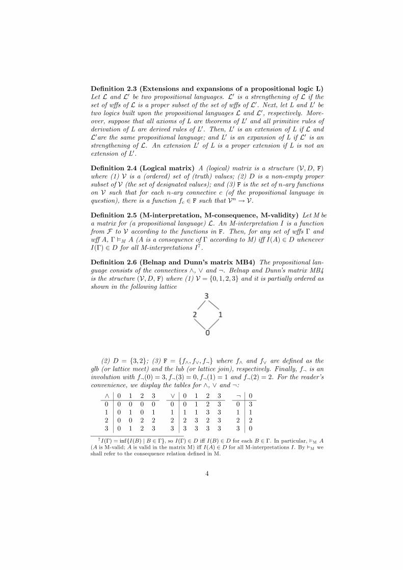
Definition 2.6 (Belnap and Dunn’s matrix MB4) The propositional lan-

guage consists of the connectives ∧, ∨ and ¬. Belnap and Dunn’s matrix MB4is the structure (V F) where (1) V = {0 1 2 3} and it is partially ordered asshown in the following lattice

(2) = {3 2}; (3) F = {∧ ∨ ¬} where ∧ and ∨ are defined as theglb (or lattice meet) and the lub (or lattice join), respectively. Finally, ¬ is aninvolution with ¬(0) = 3 ¬(3) = 0 ¬(1) = 1 and ¬(2) = 2. For the reader’sconvenience, we display the tables for ∧, ∨ and ¬:

∧ 0 1 2 30 0 0 0 01 0 1 0 12 0 0 2 23 0 1 2 3

∨ 0 1 2 30 0 1 2 31 1 1 3 32 2 3 2 33 3 3 3 3

¬ 00 31 12 23 0

7 (Γ) = inf{() | ∈ Γ}, so (Γ) ∈ iff () ∈ for each ∈ Γ. In particular, ²M

( is M-valid; is valid in the matrix M) iff () ∈ for all M-interpretations . By ²M we

shall refer to the consequence relation defined in M.

4

The notions of an MB4-interpretation, MB4-consequence and MB4-validity

are defined according to the general Definition 2.5.

The elements in MB4 can be interpreted as noted in Remark 2.7.

Remark 2.7 (On the intuitive meaning of the truth-values in MB4)

The truth values 0 1 2 and 3 can intuitively be interpreted in MB4 as follows.Let and represent truth and falsity. Then, 0 = , 1 = (either), 2 =(oth) and 3 = . Or, in terms of subsets of { }, we have: 0 = {}, 1 = ∅,2 = { } and 3 = {}.Next, the notion of a logic determined by a given matrix can be understood

as stated in the following definition.

Definition 2.8 (Logics determined by matrices) Let L be a propositionallanguage, M a matrix for L and `L a (proof theoretical) consequence relationdefined on L. Then, the logic L is determined by M iff for every set of wffs Γand wff , Γ `L iff Γ ²M . In particular, the logic L (considered as the set

of its theorems) is determined by M iff for every wff , `L iff ²M 8 .

3 Kleene’s strong 3-valued matrix with two des-

ignated elements

Kleene’s strong 3-valued matrix with two designated elements, MK3, can be

regarded as one of the sides of the lattice represented above in Definition 2.6

and it can be defined as shown in Definition 3.1.

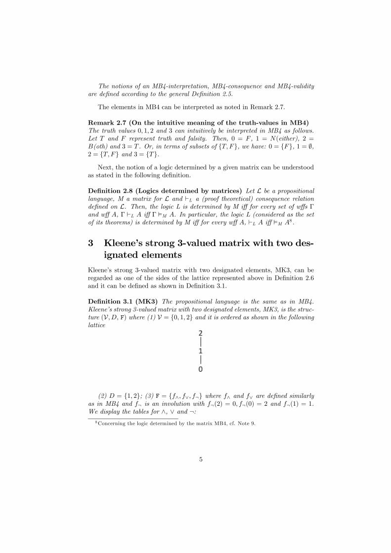
Definition 3.1 (MK3) The propositional language is the same as in MB4.

Kleene’s strong 3-valued matrix with two designated elements, MK3, is the struc-

ture (V F) where (1) V = {0 1 2} and it is ordered as shown in the followinglattice

(2) = {1 2}; (3) F = {∧ ∨ ¬} where ∧ and ∨ are defined similarlyas in MB4 and ¬ is an involution with ¬(2) = 0 ¬(0) = 2 and ¬(1) = 1.We display the tables for ∧, ∨ and ¬:

8Concerning the logic determined by the matrix MB4, cf. Note 9.

5

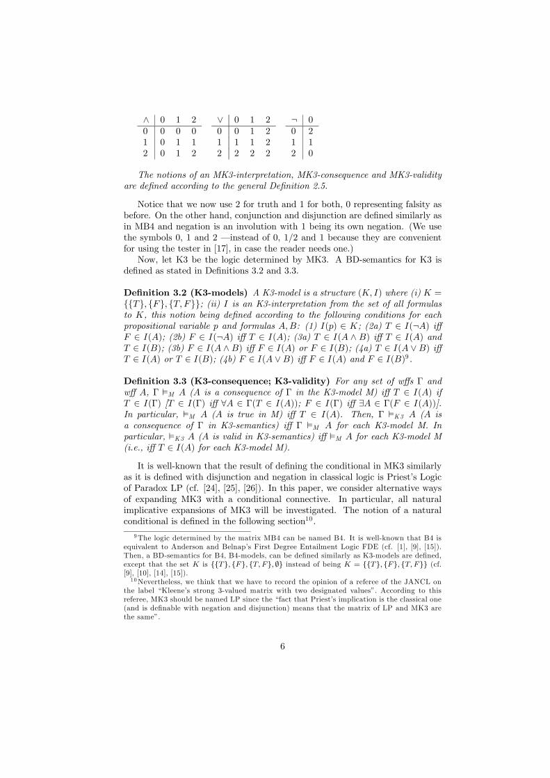
∧ 0 1 20 0 0 01 0 1 12 0 1 2

∨ 0 1 20 0 1 21 1 1 22 2 2 2

¬ 00 21 12 0

The notions of an MK3-interpretation, MK3-consequence and MK3-validity

are defined according to the general Definition 2.5.

Notice that we now use 2 for truth and 1 for both, 0 representing falsity asbefore. On the other hand, conjunction and disjunction are defined similarly as

in MB4 and negation is an involution with 1 being its own negation. (We use

the symbols 0, 1 and 2 –instead of 0, 12 and 1 because they are convenientfor using the tester in [17], in case the reader needs one.)

Now, let K3 be the logic determined by MK3. A BD-semantics for K3 is

defined as stated in Definitions 3.2 and 3.3.

Definition 3.2 (K3-models) A K3-model is a structure ( ) where (i) ={{} {} { }}; (ii) is an K3-interpretation from the set of all formulas

to , this notion being defined according to the following conditions for each

propositional variable and formulas : (1) () ∈ ; (2a) ∈ (¬) iff ∈ (); (2b) ∈ (¬) iff ∈ (); (3a) ∈ ( ∧ ) iff ∈ () and ∈ (); (3b) ∈ ( ∧) iff ∈ () or ∈ (); (4a) ∈ ( ∨) iff ∈ () or ∈ (); (4b) ∈ ( ∨) iff ∈ () and ∈ ()9 .

Definition 3.3 (K3-consequence; K3-validity) For any set of wffs Γ andwff , Γ ²M ( is a consequence of Γ in the K3-model M) iff ∈ () if ∈ (Γ) [ ∈ (Γ) iff ∀ ∈ Γ( ∈ ()); ∈ (Γ) iff ∃ ∈ Γ( ∈ ())].In particular, ²M ( is true in M) iff ∈ (). Then, Γ ²K3 ( is

a consequence of Γ in K3-semantics) iff Γ ²M for each K3-model M. In

particular, ²K3 ( is valid in K3-semantics) iff ²M for each K3-model M

(i.e., iff ∈ () for each K3-model M).

It is well-known that the result of defining the conditional in MK3 similarly

as it is defined with disjunction and negation in classical logic is Priest’s Logic

of Paradox LP (cf. [24], [25], [26]). In this paper, we consider alternative ways

of expanding MK3 with a conditional connective. In particular, all natural

implicative expansions of MK3 will be investigated. The notion of a natural

conditional is defined in the following section10.

9The logic determined by the matrix MB4 can be named B4. It is well-known that B4 is

equivalent to Anderson and Belnap’s First Degree Entailment Logic FDE (cf. [1], [9], [15]).

Then, a BD-semantics for B4, B4-models, can be defined similarly as K3-models are defined,

except that the set is {{} {} { } ∅} instead of being = {{} {} {}} (cf.[9], [10], [14], [15]).10Nevertheless, we think that we have to record the opinion of a referee of the JANCL on

the label “Kleene’s strong 3-valued matrix with two designated values”. According to this

referee, MK3 should be named LP since the “fact that Priest’s implication is the classical one

(and is definable with negation and disjunction) means that the matrix of LP and MK3 are

the same”.

6

4 Natural implicative expansions of MK3

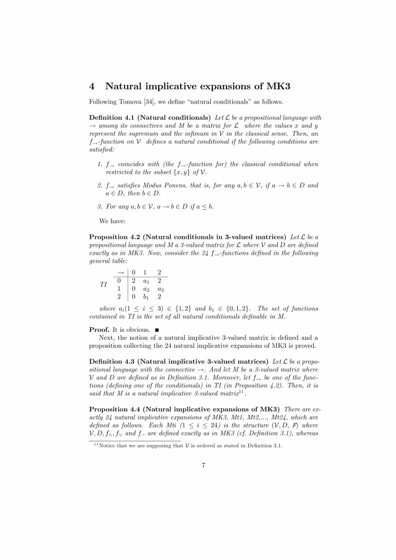
Following Tomova [34], we define “natural conditionals” as follows.

Definition 4.1 (Natural conditionals) Let L be a propositional language with→ among its connectives and M be a matrix for L where the values and

represent the supremum and the infimum in V in the classical sense. Then, an→-function on V defines a natural conditional if the following conditions are

satisfied:

1. → coincides with (the →-function for) the classical conditional whenrestricted to the subset { } of V.

2. → satisfies Modus Ponens, that is, for any ∈ V, if → ∈ and

∈ , then ∈ .

3. For any ∈ V, → ∈ if ≤ .

We have:

Proposition 4.2 (Natural conditionals in 3-valued matrices) Let L be apropositional language and M a 3-valued matrix for L where V and are defined

exactly as in MK3. Now, consider the 24 →-functions defined in the followinggeneral table:

TI

→ 0 1 20 2 1 21 0 2 32 0 1 2

where (1 ≤ ≤ 3) ∈ {1 2} and 1 ∈ {0 1 2}. The set of functions

contained in TI is the set of all natural conditionals definable in M.

Proof. It is obvious.

Next, the notion of a natural implicative 3-valued matrix is defined and a

proposition collecting the 24 natural implicative expansions of MK3 is proved.

Definition 4.3 (Natural implicative 3-valued matrices) Let L be a propo-sitional language with the connective →. And let M be a 3-valued matrix where

V and are defined as in Definition 3.1. Moreover, let → be one of the func-

tions (defining one of the conditionals) in TI (in Proposition 4.2). Then, it is

said that M is a natural implicative 3-valued matrix11 .

Proposition 4.4 (Natural implicative expansions of MK3) There are ex-

actly 24 natural implicative expansions of MK3, Mt1, Mt2,..., Mt24, which are

defined as follows. Each Mt (1 ≤ ≤ 24) is the structure (V F) whereV ∧ ∨ and ¬ are defined exactly as in MK3 (cf. Definition 3.1), whereas

11Notice that we are supposing that V is ordered as stated in Definition 3.1.

7

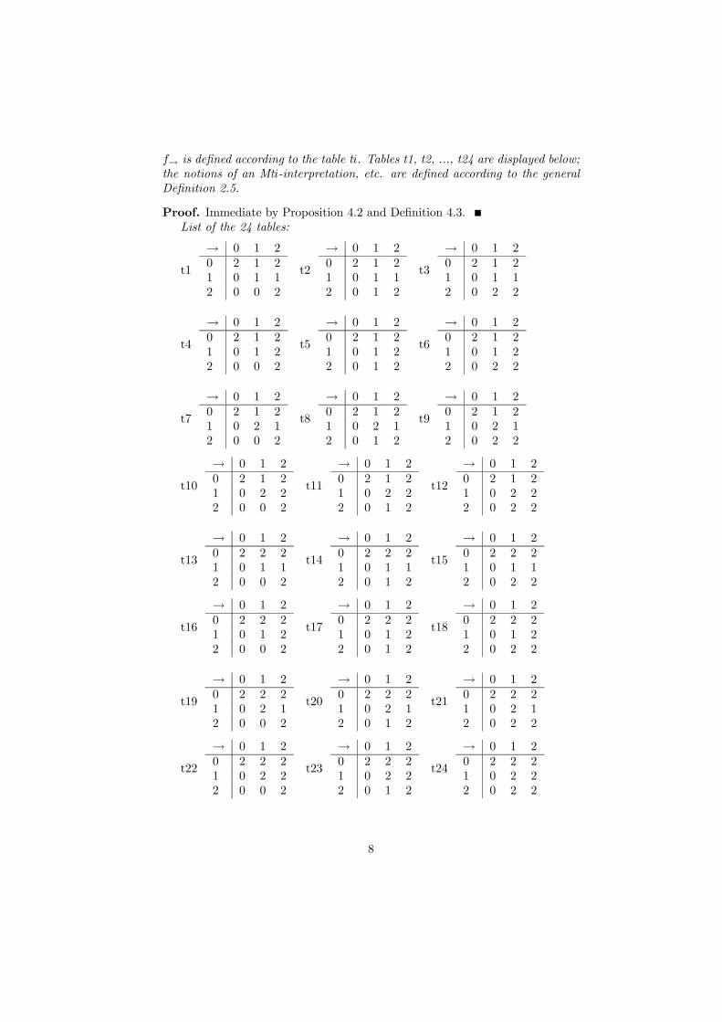
→ is defined according to the table t. Tables t1, t2, ..., t24 are displayed below;

the notions of an Mt-interpretation, etc. are defined according to the general

Definition 2.5.

Proof. Immediate by Proposition 4.2 and Definition 4.3.

List of the 24 tables:

t1

→ 0 1 20 2 1 21 0 1 12 0 0 2

t2

→ 0 1 20 2 1 21 0 1 12 0 1 2

t3

→ 0 1 20 2 1 21 0 1 12 0 2 2

t4

→ 0 1 20 2 1 21 0 1 22 0 0 2

t5

→ 0 1 20 2 1 21 0 1 22 0 1 2

t6

→ 0 1 20 2 1 21 0 1 22 0 2 2

t7

→ 0 1 20 2 1 21 0 2 12 0 0 2

t8

→ 0 1 20 2 1 21 0 2 12 0 1 2

t9

→ 0 1 20 2 1 21 0 2 12 0 2 2

t10

→ 0 1 20 2 1 21 0 2 22 0 0 2

t11

→ 0 1 20 2 1 21 0 2 22 0 1 2

t12

→ 0 1 20 2 1 21 0 2 22 0 2 2

t13

→ 0 1 20 2 2 21 0 1 12 0 0 2

t14

→ 0 1 20 2 2 21 0 1 12 0 1 2

t15

→ 0 1 20 2 2 21 0 1 12 0 2 2

t16

→ 0 1 20 2 2 21 0 1 22 0 0 2

t17

→ 0 1 20 2 2 21 0 1 22 0 1 2

t18

→ 0 1 20 2 2 21 0 1 22 0 2 2

t19

→ 0 1 20 2 2 21 0 2 12 0 0 2

t20

→ 0 1 20 2 2 21 0 2 12 0 1 2

t21

→ 0 1 20 2 2 21 0 2 12 0 2 2

t22

→ 0 1 20 2 2 21 0 2 22 0 0 2

t23

→ 0 1 20 2 2 21 0 2 22 0 1 2

t24

→ 0 1 20 2 2 21 0 2 22 0 2 2

8

The aim of this paper is to provide an overdetermined BD-semantics for the

logic Lt characterized by each matrix Mt (1 ≤ ≤ 24)12 .

5 The basic logics b3, b31, b32

In this section, the basic logics b3, b31, b32 are defined and some of their properties

are proved. The logic b3 is axiomatized as follows (the label is intended to

abbreviate “basic logic contained in all natural implicative expansions of K3”).

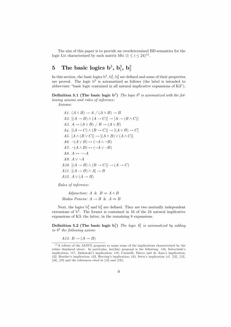
Definition 5.1 (The basic logic b3) The logic b3 is axiomatized with the fol-

lowing axioms and rules of inference:

Axioms:

A1. ( ∧)→ / ( ∧)→

A2. [(→ ) ∧ (→ )]→ [→ ( ∧ )]A3. → ( ∨) / → ( ∨)A4. [(→ ) ∧ ( → )]→ [( ∨)→ ]

A5. [ ∧ ( ∨)]→ [( ∧) ∨ ( ∧ )]A6. ¬( ∨)↔ (¬ ∧ ¬)A7. ¬( ∧)↔ (¬ ∨ ¬)A8. ↔ ¬¬A9. ∨ ¬A10. [(→ ) ∧ ( → )]→ (→ )

A11. [(→ ) ∧]→

A12. ∨ (→ )

Rules of inference:

Adjunction: & ⇒ ∧Modus Ponens: → & ⇒

Next, the logics b31 and b32 are defined. They are two mutually independent

extensions of b3. The former is contained in 16 of the 24 natural implicative

expansions of K3; the latter, in the remaining 8 expansions.

Definition 5.2 (The basic logic b31) The logic b31 is axiomatized by adding

to b3 the following axiom:

A13. → (→ )

12A referee of the JANCL proposes to name some of the implications characterized by the

tables displayed above. In particular, her(his) proposal is the following: t16, Sobocinski’s

implication; t17, Jáskowski’s implication; t18, Carnielli, Marco and de Amo’s implication;

t22, Rescher’s implication; t23, Heyting’s implication; t24, Sette’s implication (cf. [12], [13],

[16], [19] and the references cited in [13] and [19]).

9

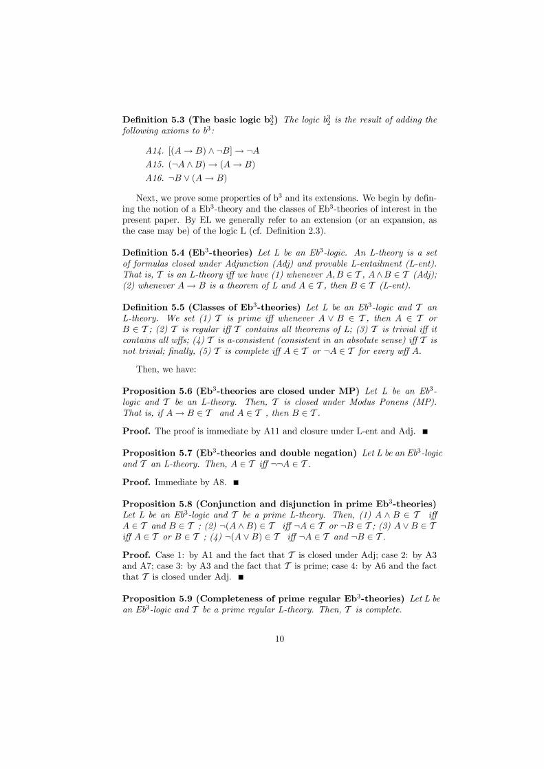
Definition 5.3 (The basic logic b32) The logic b32 is the result of adding the

following axioms to b3:

A14. [(→ ) ∧ ¬]→ ¬A15. (¬ ∧)→ (→ )

A16. ¬ ∨ (→ )

Next, we prove some properties of b3 and its extensions. We begin by defin-

ing the notion of a Eb3-theory and the classes of Eb3-theories of interest in the

present paper. By EL we generally refer to an extension (or an expansion, as

the case may be) of the logic L (cf. Definition 2.3).

Definition 5.4 (Eb3-theories) Let L be an Eb3-logic. An L-theory is a set

of formulas closed under Adjunction (Adj) and provable L-entailment (L-ent).

That is, T is an L-theory iff we have (1) whenever ∈ T , ∧ ∈ T (Adj);

(2) whenever → is a theorem of L and ∈ T , then ∈ T (L-ent).

Definition 5.5 (Classes of Eb3-theories) Let L be an Eb3-logic and T an

L-theory. We set (1) T is prime iff whenever ∨ ∈ T , then ∈ T or

∈ T ; (2) T is regular iff T contains all theorems of L; (3) T is trivial iff it

contains all wffs; (4) T is a-consistent (consistent in an absolute sense) iff T isnot trivial; finally, (5) T is complete iff ∈ T or ¬ ∈ T for every wff .

Then, we have:

Proposition 5.6 (Eb3-theories are closed under MP) Let L be an Eb3-

logic and T be an L-theory. Then, T is closed under Modus Ponens (MP).

That is, if → ∈ T and ∈ T , then ∈ T .Proof. The proof is immediate by A11 and closure under L-ent and Adj.

Proposition 5.7 (Eb3-theories and double negation) Let L be an Eb3-logic

and T an L-theory. Then, ∈ T iff ¬¬ ∈ T .Proof. Immediate by A8.

Proposition 5.8 (Conjunction and disjunction in prime Eb3-theories)

Let L be an Eb3-logic and T be a prime L-theory. Then, (1) ∧ ∈ T iff

∈ T and ∈ T ; (2) ¬( ∧) ∈ T iff ¬ ∈ T or ¬ ∈ T ; (3) ∨ ∈ Tiff ∈ T or ∈ T ; (4) ¬( ∨) ∈ T iff ¬ ∈ T and ¬ ∈ T .Proof. Case 1: by A1 and the fact that T is closed under Adj; case 2: by A3

and A7; case 3: by A3 and the fact that T is prime; case 4: by A6 and the factthat T is closed under Adj.

Proposition 5.9 (Completeness of prime regular Eb3-theories) Let L be

an Eb3-logic and T be a prime regular L-theory. Then, T is complete.

10

Proof. Immediate by A9.

Next, we remark some properties of Eb31-theories and Eb32-theories.

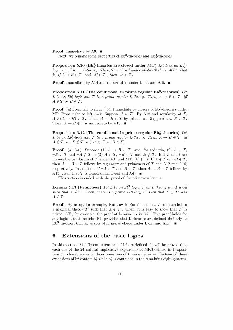
Proposition 5.10 (Eb32-theories are closed under MT) Let L be an Eb32-

logic and T be an L-theory. Then, T is closed under Modus Tollens (MT). Thatis, if → ∈ T and ¬ ∈ T , then ¬ ∈ T .Proof. Immediate by A14 and closure of T under L-ent and Adj.

Proposition 5.11 (The conditional in prime regular Eb31-theories) Let

L be an Eb31-logic and T be a prime regular L-theory. Then, → ∈ T iff

∈ T or ∈ T .Proof. (a) From left to right (⇒): Immediate by closure of Eb3-theories underMP. From right to left (⇐): Suppose ∈ T . By A12 and regularity of T , ∨ ( → ) ∈ T . Then, → ∈ T by primeness. Suppose now ∈ T .Then, → ∈ T is immediate by A13.

Proposition 5.12 (The conditional in prime regular Eb32-theories) Let

L be an Eb32-logic and T be a prime regular L-theory. Then, → ∈ T iff

∈ T or ¬ ∈ T or (¬ ∈ T & ∈ T ).Proof. (a) (⇒): Suppose (1) → ∈ T and, for reductio, (2) ∈ T ,¬ ∈ T and ¬ ∈ T or (3) ∈ T , ¬ ∈ T and ∈ T . But 2 and 3 areimpossible by closure of T under MP and MT. (b) (⇐): If ∈ T or ¬ ∈ T ,then → ∈ T follows by regularity and primeness of T and A12 and A16,

respectively. In addition, if ¬ ∈ T and ∈ T , then → ∈ T follows by

A15, given that T is closed under L-ent and Adj.

This section is ended with the proof of the primeness lemma.

Lemma 5.13 (Primeness) Let L be an Eb3-logic, T an L-theory and a wff

such that ∈ T . Then, there is a prime L-theory T 0 such that T ⊆ T 0 and ∈ T 0.Proof. By using, for example, Kuratowski-Zorn’s Lemma, T is extended to

a maximal theory T 0 such that ∈ T 0. Then, it is easy to show that T 0 isprime. (Cf., for example, the proof of Lemma 5.7 in [22]. This proof holds for

any logic L that includes B4, provided that L-theories are defined similarly as

Eb3-theories, that is, as sets of formulas closed under L-ent and Adj).

6 Extensions of the basic logics

In this section, 24 different extensions of b3 are defined. It will be proved that

each one of the 24 natural implicative expansions of MK3 defined in Proposi-

tion 3.4 characterizes or determines one of these extensions. Sixteen of these

extensions of b3 contain b31 while b32 is contained in the remaining eight systems.

11

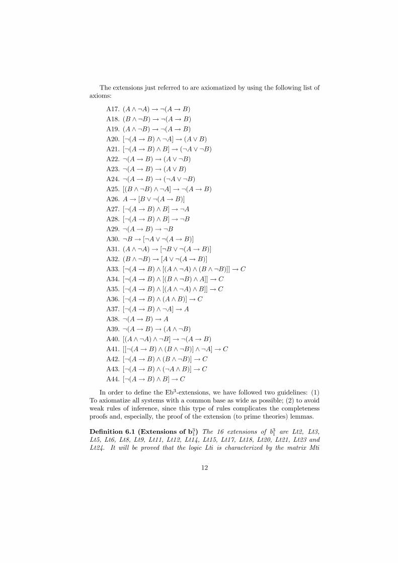
The extensions just referred to are axiomatized by using the following list of

axioms:

A17. ( ∧ ¬)→ ¬(→ )

A18. ( ∧ ¬)→ ¬(→ )

A19. ( ∧ ¬)→ ¬(→ )

A20. [¬(→ ) ∧ ¬]→ ( ∨)A21. [¬(→ ) ∧]→ (¬ ∨ ¬)A22. ¬(→ )→ ( ∨ ¬)A23. ¬(→ )→ ( ∨)A24. ¬(→ )→ (¬ ∨ ¬)A25. [( ∧ ¬) ∧ ¬]→ ¬(→ )

A26. → [ ∨ ¬(→ )]

A27. [¬(→ ) ∧]→ ¬A28. [¬(→ ) ∧]→ ¬A29. ¬(→ )→ ¬A30. ¬ → [¬ ∨ ¬(→ )]

A31. ( ∧ ¬)→ [¬ ∨ ¬(→ )]

A32. ( ∧ ¬)→ [ ∨ ¬(→ )]

A33. [¬(→ ) ∧ [( ∧ ¬) ∧ ( ∧ ¬)]]→

A34. [¬(→ ) ∧ [( ∧ ¬) ∧]]→

A35. [¬(→ ) ∧ [( ∧ ¬) ∧]]→

A36. [¬(→ ) ∧ ( ∧)]→

A37. [¬(→ ) ∧ ¬]→

A38. ¬(→ )→

A39. ¬(→ )→ ( ∧ ¬)A40. [( ∧ ¬) ∧ ¬]→ ¬(→ )

A41. [[¬(→ ) ∧ ( ∧ ¬)] ∧ ¬]→

A42. [¬(→ ) ∧ ( ∧ ¬)]→

A43. [¬(→ ) ∧ (¬ ∧)]→

A44. [¬(→ ) ∧]→

In order to define the Eb3-extensions, we have followed two guidelines: (1)

To axiomatize all systems with a common base as wide as possible; (2) to avoid

weak rules of inference, since this type of rules complicates the completeness

proofs and, especially, the proof of the extension (to prime theories) lemmas.

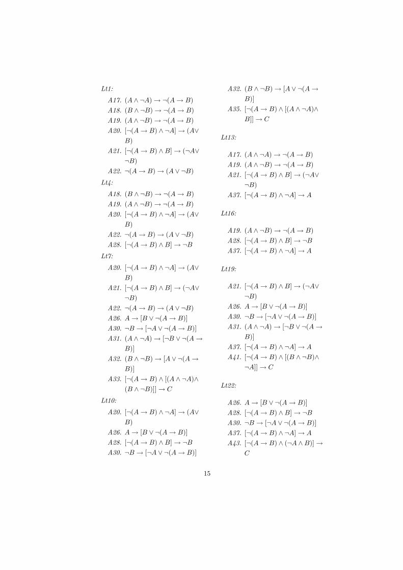
Definition 6.1 (Extensions of b31) The 16 extensions of b31 are Lt2, Lt3,

Lt5, Lt6, Lt8, Lt9, Lt11, Lt12, Lt14, Lt15, Lt17, Lt18, Lt20, Lt21, Lt23 and

Lt24. It will be proved that the logic Lt is characterized by the matrix Mt

12

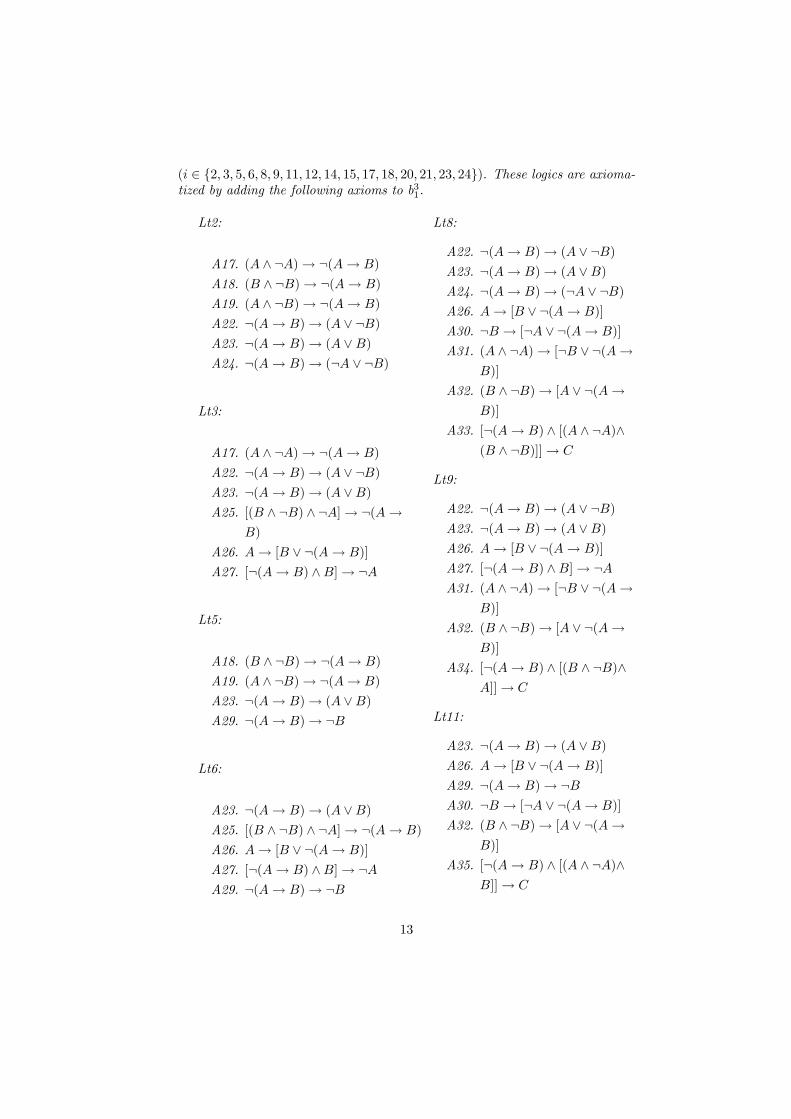
( ∈ {2 3 5 6 8 9 11 12 14 15 17 18 20 21 23 24}). These logics are axioma-tized by adding the following axioms to b31.

Lt2:

A17. ( ∧ ¬)→ ¬(→ )

A18. ( ∧ ¬)→ ¬(→ )

A19. ( ∧ ¬)→ ¬(→ )

A22. ¬(→ )→ ( ∨ ¬)A23. ¬(→ )→ ( ∨)A24. ¬(→ )→ (¬ ∨ ¬)

Lt3:

A17. ( ∧ ¬)→ ¬(→ )

A22. ¬(→ )→ ( ∨ ¬)A23. ¬(→ )→ ( ∨)A25. [( ∧ ¬) ∧ ¬]→ ¬(→

)

A26. → [ ∨ ¬(→ )]

A27. [¬(→ ) ∧]→ ¬

Lt5:

A18. ( ∧ ¬)→ ¬(→ )

A19. ( ∧ ¬)→ ¬(→ )

A23. ¬(→ )→ ( ∨)A29. ¬(→ )→ ¬

Lt6:

A23. ¬(→ )→ ( ∨)A25. [( ∧ ¬) ∧ ¬]→ ¬(→ )

A26. → [ ∨ ¬(→ )]

A27. [¬(→ ) ∧]→ ¬A29. ¬(→ )→ ¬

Lt8:

A22. ¬(→ )→ ( ∨ ¬)A23. ¬(→ )→ ( ∨)A24. ¬(→ )→ (¬ ∨ ¬)A26. → [ ∨ ¬(→ )]

A30. ¬ → [¬ ∨ ¬(→ )]

A31. ( ∧ ¬)→ [¬ ∨ ¬(→)]

A32. ( ∧ ¬)→ [ ∨ ¬(→)]

A33. [¬(→ ) ∧ [( ∧ ¬)∧( ∧ ¬)]]→

Lt9:

A22. ¬(→ )→ ( ∨ ¬)A23. ¬(→ )→ ( ∨)A26. → [ ∨ ¬(→ )]

A27. [¬(→ ) ∧]→ ¬A31. ( ∧ ¬)→ [¬ ∨ ¬(→

)]

A32. ( ∧ ¬)→ [ ∨ ¬(→)]

A34. [¬(→ ) ∧ [( ∧ ¬)∧]]→

Lt11:

A23. ¬(→ )→ ( ∨)A26. → [ ∨ ¬(→ )]

A29. ¬(→ )→ ¬A30. ¬ → [¬ ∨ ¬(→ )]

A32. ( ∧ ¬)→ [ ∨ ¬(→)]

A35. [¬(→ ) ∧ [( ∧ ¬)∧]]→

13

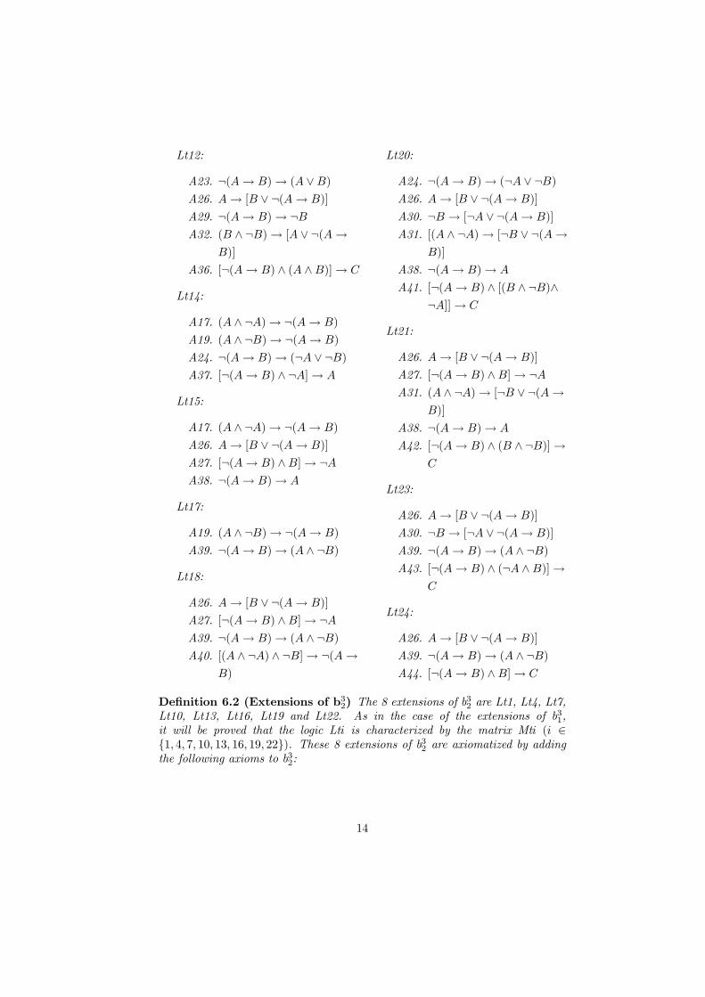
Lt12:

A23. ¬(→ )→ ( ∨)A26. → [ ∨ ¬(→ )]

A29. ¬(→ )→ ¬A32. ( ∧ ¬)→ [ ∨ ¬(→

)]

A36. [¬(→ ) ∧ ( ∧)]→

Lt14:

A17. ( ∧ ¬)→ ¬(→ )

A19. ( ∧ ¬)→ ¬(→ )

A24. ¬(→ )→ (¬ ∨ ¬)A37. [¬(→ ) ∧ ¬]→

Lt15:

A17. ( ∧ ¬)→ ¬(→ )

A26. → [ ∨ ¬(→ )]

A27. [¬(→ ) ∧]→ ¬A38. ¬(→ )→

Lt17:

A19. ( ∧ ¬)→ ¬(→ )

A39. ¬(→ )→ ( ∧ ¬)

Lt18:

A26. → [ ∨ ¬(→ )]

A27. [¬(→ ) ∧]→ ¬A39. ¬(→ )→ ( ∧ ¬)A40. [( ∧ ¬) ∧ ¬]→ ¬(→

)

Lt20:

A24. ¬(→ )→ (¬ ∨ ¬)A26. → [ ∨ ¬(→ )]

A30. ¬ → [¬ ∨ ¬(→ )]

A31. [( ∧ ¬)→ [¬ ∨ ¬(→)]

A38. ¬(→ )→

A41. [¬(→ ) ∧ [( ∧ ¬)∧¬]]→

Lt21:

A26. → [ ∨ ¬(→ )]

A27. [¬(→ ) ∧]→ ¬A31. ( ∧ ¬)→ [¬ ∨ ¬(→

)]

A38. ¬(→ )→

A42. [¬(→ ) ∧ ( ∧ ¬)]→

Lt23:

A26. → [ ∨ ¬(→ )]

A30. ¬ → [¬ ∨ ¬(→ )]

A39. ¬(→ )→ ( ∧ ¬)A43. [¬(→ ) ∧ (¬ ∧)]→

Lt24:

A26. → [ ∨ ¬(→ )]

A39. ¬(→ )→ ( ∧ ¬)A44. [¬(→ ) ∧]→

Definition 6.2 (Extensions of b32) The 8 extensions of b32 are Lt1, Lt4, Lt7,

Lt10, Lt13, Lt16, Lt19 and Lt22. As in the case of the extensions of b31,

it will be proved that the logic Lt is characterized by the matrix Mt ( ∈{1 4 7 10 13 16 19 22}). These 8 extensions of b32 are axiomatized by addingthe following axioms to b32:

14

Lt1:

A17. ( ∧ ¬)→ ¬(→ )

A18. ( ∧ ¬)→ ¬(→ )

A19. ( ∧ ¬)→ ¬(→ )

A20. [¬(→ ) ∧ ¬]→ (∨)

A21. [¬(→ ) ∧]→ (¬∨¬)

A22. ¬(→ )→ ( ∨ ¬)Lt4:

A18. ( ∧ ¬)→ ¬(→ )

A19. ( ∧ ¬)→ ¬(→ )

A20. [¬(→ ) ∧ ¬]→ (∨)

A22. ¬(→ )→ ( ∨ ¬)A28. [¬(→ ) ∧]→ ¬

Lt7:

A20. [¬(→ ) ∧ ¬]→ (∨)

A21. [¬(→ ) ∧]→ (¬∨¬)

A22. ¬(→ )→ ( ∨ ¬)A26. → [ ∨ ¬(→ )]

A30. ¬ → [¬ ∨ ¬(→ )]

A31. ( ∧ ¬)→ [¬ ∨ ¬(→)]

A32. ( ∧ ¬)→ [ ∨ ¬(→)]

A33. [¬(→ ) ∧ [( ∧ ¬)∧( ∧ ¬)]]→

Lt10:

A20. [¬(→ ) ∧ ¬]→ (∨)

A26. → [ ∨ ¬(→ )]

A28. [¬(→ ) ∧]→ ¬A30. ¬ → [¬ ∨ ¬(→ )]

A32. ( ∧ ¬)→ [ ∨ ¬(→)]

A35. [¬(→ ) ∧ [( ∧ ¬)∧]]→

Lt13:

A17. ( ∧ ¬)→ ¬(→ )

A19. ( ∧ ¬)→ ¬(→ )

A21. [¬(→ ) ∧]→ (¬∨¬)

A37. [¬(→ ) ∧ ¬]→

Lt16:

A19. ( ∧ ¬)→ ¬(→ )

A28. [¬(→ ) ∧]→ ¬A37. [¬(→ ) ∧ ¬]→

Lt19:

A21. [¬(→ ) ∧]→ (¬∨¬)

A26. → [ ∨ ¬(→ )]

A30. ¬ → [¬ ∨ ¬(→ )]

A31. ( ∧ ¬)→ [¬ ∨ ¬(→)]

A37. [¬(→ ) ∧ ¬]→

A41. [¬(→ ) ∧ [( ∧ ¬)∧¬]]→

Lt22:

A26. → [ ∨ ¬(→ )]

A28. [¬(→ ) ∧]→ ¬A30. ¬ → [¬ ∨ ¬(→ )]

A37. [¬(→ ) ∧ ¬]→

A43. [¬(→ ) ∧ (¬ ∧)]→

15

In what follows, we prove two important propositions on the behavior of

negated conditionals in the extensions of b31 and b32 just defined.

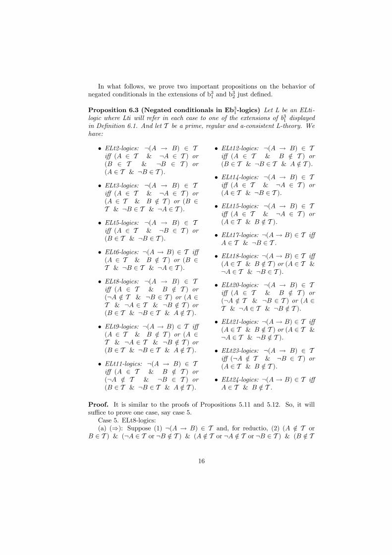
Proposition 6.3 (Negated conditionals in Eb31-logics) Let L be an ELt-

logic where Lt will refer in each case to one of the extensions of b31 displayed

in Definition 6.1. And let T be a prime, regular and a-consistent L-theory. We

have:

• ELt2-logics: ¬( → ) ∈ Tiff ( ∈ T & ¬ ∈ T ) or( ∈ T & ¬ ∈ T ) or( ∈ T & ¬ ∈ T ).

• ELt3-logics: ¬( → ) ∈ Tiff ( ∈ T & ¬ ∈ T ) or( ∈ T & ∈ T ) or ( ∈T & ¬ ∈ T & ¬ ∈ T ).

• ELt5-logics: ¬( → ) ∈ Tiff ( ∈ T & ¬ ∈ T ) or( ∈ T & ¬ ∈ T ).

• ELt6-logics: ¬( → ) ∈ T iff

( ∈ T & ∈ T ) or ( ∈T & ¬ ∈ T & ¬ ∈ T ).

• ELt8-logics: ¬( → ) ∈ Tiff ( ∈ T & ∈ T ) or(¬ ∈ T & ¬ ∈ T ) or ( ∈T & ¬ ∈ T & ¬ ∈ T ) or( ∈ T & ¬ ∈ T & ∈ T ).

• ELt9-logics: ¬( → ) ∈ T iff

( ∈ T & ∈ T ) or ( ∈T & ¬ ∈ T & ¬ ∈ T ) or( ∈ T & ¬ ∈ T & ∈ T ).

• ELt11-logics: ¬( → ) ∈ Tiff ( ∈ T & ∈ T ) or(¬ ∈ T & ¬ ∈ T ) or( ∈ T & ¬ ∈ T & ∈ T ).

• ELt12-logics: ¬( → ) ∈ Tiff ( ∈ T & ∈ T ) or( ∈ T & ¬ ∈ T & ∈ T ).

• ELt14-logics: ¬( → ) ∈ Tiff ( ∈ T & ¬ ∈ T ) or( ∈ T & ¬ ∈ T ).

• ELt15-logics: ¬( → ) ∈ Tiff ( ∈ T & ¬ ∈ T ) or( ∈ T & ∈ T ).

• ELt17-logics: ¬( → ) ∈ T iff

∈ T & ¬ ∈ T .• ELt18-logics: ¬( → ) ∈ T iff

( ∈ T & ∈ T ) or ( ∈ T &¬ ∈ T & ¬ ∈ T ).

• ELt20-logics: ¬( → ) ∈ Tiff ( ∈ T & ∈ T ) or(¬ ∈ T & ¬ ∈ T ) or ( ∈T & ¬ ∈ T & ¬ ∈ T ).

• ELt21-logics: ¬( → ) ∈ T iff

( ∈ T & ∈ T ) or ( ∈ T &¬ ∈ T & ¬ ∈ T ).

• ELt23-logics: ¬( → ) ∈ Tiff (¬ ∈ T & ¬ ∈ T ) or( ∈ T & ∈ T ).

• ELt24-logics: ¬( → ) ∈ T iff

∈ T & ∈ T .

Proof. It is similar to the proofs of Propositions 5.11 and 5.12. So, it will

suffice to prove one case, say case 5.

Case 5. ELt8-logics:

(a) (⇒): Suppose (1) ¬( → ) ∈ T and, for reductio, (2) ( ∈ T or

∈ T ) & (¬ ∈ T or ¬ ∈ T ) & ( ∈ T or ¬ ∈ T or ¬ ∈ T ) & ( ∈ T

16

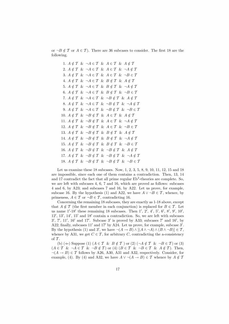
or ¬ ∈ T or ∈ T ). There are 36 subcases to consider. The first 18 are thefollowing.

1. ∈ T & ¬ ∈ T & ∈ T & ∈ T2. ∈ T & ¬ ∈ T & ∈ T & ¬ ∈ T3. ∈ T & ¬ ∈ T & ∈ T & ¬ ∈ T4. ∈ T & ¬ ∈ T & ∈ T & ∈ T5. ∈ T & ¬ ∈ T & ∈ T & ¬ ∈ T6. ∈ T & ¬ ∈ T & ∈ T & ¬ ∈ T7. ∈ T & ¬ ∈ T & ¬ ∈ T & ∈ T8. ∈ T & ¬ ∈ T & ¬ ∈ T & ¬ ∈ T9. ∈ T & ¬ ∈ T & ¬ ∈ T & ¬ ∈ T10. ∈ T & ¬ ∈ T & ∈ T & ∈ T11. ∈ T & ¬ ∈ T & ∈ T & ¬ ∈ T12. ∈ T & ¬ ∈ T & ∈ T & ¬ ∈ T13. ∈ T & ¬ ∈ T & ∈ T & ∈ T14. ∈ T & ¬ ∈ T & ∈ T & ¬ ∈ T15. ∈ T & ¬ ∈ T & ∈ T & ¬ ∈ T16. ∈ T & ¬ ∈ T & ¬ ∈ T & ∈ T17. ∈ T & ¬ ∈ T & ¬ ∈ T & ¬ ∈ T18. ∈ T & ¬ ∈ T & ¬ ∈ T & ¬ ∈ T

Let us examine these 18 subcases. Now, 1, 2, 3, 5, 8, 9, 10, 11, 12, 15 and 18

are impossible, since each one of them contains a contradiction. Then, 13, 14

and 17 contradict the fact that all prime regular Eb3-theories are complete. So,

we are left with subcases 4, 6, 7 and 16, which are proved as follows: subcases

4 and 6, by A23; and subcases 7 and 16, by A22. Let us prove, for example,

subcase 16. By the hypothesis (1) and A22, we have ∨ ¬ ∈ T , whence, byprimeness, ∈ T or ¬ ∈ T , contradicting 16.Concerning the remaining 18 subcases, they are exactly as 1-18 above, except

that ∈ T (the first member in each conjunction) is replaced for ∈ T . Letus name 10-180 these remaining 18 subcases. Then 10, 20, 40, 50, 60, 80, 90, 100,120, 130, 140, 150 and 180 contain a contradiction. So, we are left with subcases30, 70, 110, 160 and 170. Subcase 30 is proved by A33; subcases 70 and 160, byA22; finally, subcases 110 and 170 by A24. Let us prove, for example, subcase 30.By the hypothesis (1) and 30, we have ¬(→ )∧ [(∧¬)∧ ( ∧¬)] ∈ T ,whence by A31, we get ∈ T , for arbitrary , contradicting the a-consistencyof T .(b) (⇐) Suppose (1) ( ∈ T & ∈ T ) or (2) (¬ ∈ T & ¬ ∈ T ) or (3)

( ∈ T & ¬ ∈ T & ¬ ∈ T ) or (4) ( ∈ T & ¬ ∈ T & ∈ T ). Then,¬( → ) ∈ T follows by A26, A30, A31 and A32, respectively. Consider, for

example, (4). By (4) and A32, we have ∨ ¬( → ) ∈ T whence by ∈ T

17

and primeness of T , ¬(→ ) ∈ T follows.

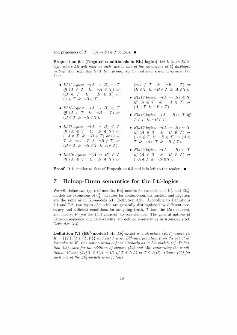
Proposition 6.4 (Negated conditionals in Eb32-logics) Let L be an ELt-

logic where Lt will refer in each case to one of the extensions of b32 displayed

in Definition 6.2. And let T be a prime, regular and a-consistent L-theory. We

have:

• ELt1-logics: ¬( → ) ∈ Tiff ( ∈ T & ¬ ∈ T ) or( ∈ T & ¬ ∈ T ) or( ∈ T & ¬ ∈ T ).

• ELt4-logics: ¬( → ) ∈ Tiff ( ∈ T & ¬ ∈ T ) or( ∈ T & ¬ ∈ T ).

• ELt7-logics: ¬( → ) ∈ Tiff ( ∈ T & ∈ T ) or(¬ ∈ T & ¬ ∈ T ) or ( ∈T & ¬ ∈ T & ¬ ∈ T ) or( ∈ T & ¬ ∈ T & ∈ T ).

• ELt10-logics: ¬( → ) ∈ Tiff ( ∈ T & ∈ T ) or

(¬ ∈ T & ¬ ∈ T ) or( ∈ T & ¬ ∈ T & ∈ T ).

• ELt13-logics: ¬( → ) ∈ Tiff ( ∈ T & ¬ ∈ T ) or( ∈ T & ¬ ∈ T ).

• ELt16-logics: ¬( → ) ∈ iff

∈ & ¬ ∈ .

• ELt19-logics: ¬( → ) ∈ Tiff ( ∈ T & ∈ T ) or(¬ ∈ T & ¬ ∈ T ) or ( ∈T & ¬ ∈ T & ¬ ∈ T ).

• ELt22-logics: ¬( → ) ∈ Tiff ( ∈ T & ∈ T ) or(¬ ∈ T & ¬ ∈ T ).

Proof. It is similar to that of Proposition 6.3 and it is left to the reader.

7 Belnap-Dunn semantics for the Lt-logics

We will define two types of models: Eb31-models for extensions of b31, and Eb

32-

models for extensions of b32 . Clauses for conjunction, disjunction and negation

are the same as in K3-models (cf. Definition 3.2). According to Definitions

7.1 and 7.2, two types of models are generally distinguished by different nec-

essary and suficient conditions for assigning truth, (see the (5a) clauses),

and falsity, (see the (5b) clauses), to conditionals. The general notions of

ELt-consequence and ELt-validity are defined similarly as in K3-models (cf.

Definition 3.3).

Definition 7.1 (Eb31-models) An Eb31-model is a structure ( ) where (i)

= {{} {} { }} and (ii) is an Eb31-interpretation from the set of all

formulas to , this notion being defined similarly as in K3-models (cf. Defini-

tion 3.2), save for the addition of clauses (5a) and (5b) concerning the condi-

tional. Clause (5a) ∈ ( → ) iff ∈ () or ∈ (). Clause (5b) foreach one of the Eb31-models is as follows:

18

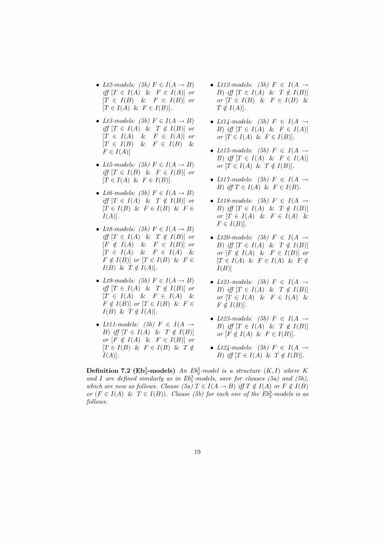
• Lt2-models: (5b) ∈ ( → )iff [ ∈ () & ∈ ()] or[ ∈ () & ∈ ()] or[ ∈ () & ∈ ()].

• Lt3-models: (5b) ∈ ( → )iff [ ∈ () & ∈ ()] or[ ∈ () & ∈ ()] or[ ∈ () & ∈ () & ∈ ()]

• Lt5-models: (5b) ∈ ( → )iff [ ∈ () & ∈ ()] or[ ∈ () & ∈ ()]

• Lt6-models: (5b) ∈ ( → )iff [ ∈ () & ∈ ()] or[ ∈ () & ∈ () & ∈()].

• Lt8-models: (5b) ∈ ( → )iff [ ∈ () & ∈ ()] or[ ∈ () & ∈ ()] or[ ∈ () & ∈ () & ∈ ()] or [ ∈ () & ∈() & ∈ ()].

• Lt9-models: (5b) ∈ ( → )iff [ ∈ () & ∈ ()] or[ ∈ () & ∈ () & ∈ ()] or [ ∈ () & ∈() & ∈ ()].

• Lt11-models: (5b) ∈ ( →) iff [ ∈ () & ∈ ()]or [ ∈ () & ∈ ()] or[ ∈ () & ∈ () & ∈()].

• Lt12-models: (5b) ∈ ( →) iff [ ∈ () & ∈ ()]or [ ∈ () & ∈ () & ∈ ()].

• Lt14-models: (5b) ∈ ( →) iff [ ∈ () & ∈ ()]or [ ∈ () & ∈ ()].

• Lt15-models: (5b) ∈ ( →) iff [ ∈ () & ∈ ()]or [ ∈ () & ∈ ()].

• Lt17-models: (5b) ∈ ( →) iff ∈ () & ∈ ().

• Lt18-models: (5b) ∈ ( →) iff [ ∈ () & ∈ ()]or [ ∈ () & ∈ () & ∈ ()].

• Lt20-models: (5b) ∈ ( →) iff [ ∈ () & ∈ ()]or [ ∈ () & ∈ ()] or[ ∈ () & ∈ () & ∈()]

• Lt21-models: (5b) ∈ ( →) iff [ ∈ () & ∈ ()]or [ ∈ () & ∈ () & ∈ ()].

• Lt23-models: (5b) ∈ ( →) iff [ ∈ () & ∈ ()]or [ ∈ () & ∈ ()].

• Lt24-models: (5b) ∈ ( →) iff [ ∈ () & ∈ ()].

Definition 7.2 (Eb32-models) An Eb32-model is a structure ( ) where

and are defined similarly as in Eb31-models, save for clauses (5a) and (5b),

which are now as follows. Clause (5a) ∈ (→ ) iff ∈ () or ∈ ()or ( ∈ () & ∈ ()). Clause (5b) for each one of the Eb32-models is asfollows:

19

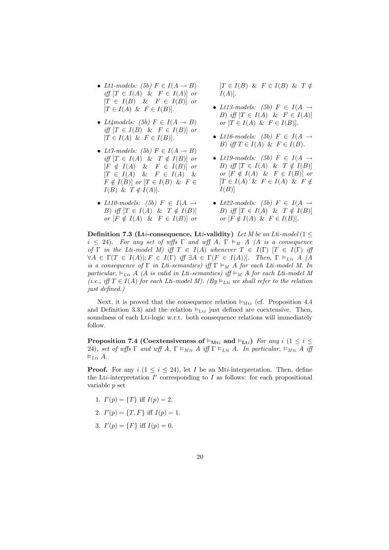
• Lt1-models: (5b) ∈ ( → )iff [ ∈ () & ∈ ()] or[ ∈ () & ∈ ()] or[ ∈ () & ∈ ()].

• Lt4models: (5b) ∈ ( → )iff [ ∈ () & ∈ ()] or[ ∈ () & ∈ ()].

• Lt7-models: (5b) ∈ ( → )iff [ ∈ () & ∈ ()] or[ ∈ () & ∈ ()] or[ ∈ () & ∈ () & ∈ ()] or [ ∈ () & ∈() & ∈ ()].

• Lt10-models: (5b) ∈ ( →) iff [ ∈ () & ∈ ()]or [ ∈ () & ∈ ()] or

[ ∈ () & ∈ () & ∈()].

• Lt13-models: (5b) ∈ ( →) iff [ ∈ () & ∈ ()]or [ ∈ () & ∈ ()].

• Lt16-models: (5b) ∈ ( →) iff ∈ () & ∈ ().

• Lt19-models: (5b) ∈ ( →) iff [ ∈ () & ∈ ()]or [ ∈ () & ∈ ()] or[ ∈ () & ∈ () & ∈()]

• Lt22-models: (5b) ∈ ( →) iff [ ∈ () & ∈ ()]or [ ∈ () & ∈ ()].

Definition 7.3 (Lt-consequence, Lt-validity) Let M be an Lt-model (1 ≤ ≤ 24). For any set of wffs Γ and wff , Γ ²M ( is a consequence

of Γ in the Lt-model M) iff ∈ () whenever ∈ (Γ) [ ∈ (Γ) iff∀ ∈ Γ( ∈ ()); ∈ (Γ) iff ∃ ∈ Γ( ∈ ())]. Then, Γ ²Lt (

is a consequence of Γ in Lt-semantics) iff Γ ²M for each Lt-model M. In

particular, ²Lt ( is valid in Lt-semantics) iff ²M for each Lt-model M

(i.e., iff ∈ () for each Lt-model M). (By ²Lt we shall refer to the relationjust defined.)

Next, it is proved that the consequence relation ²Mt (cf. Proposition 4.4and Definition 3.3) and the relation ²Lt just defined are coextensive. Then,soundness of each Lt-logic w.r.t. both consequence relations will immediately

follow.

Proposition 7.4 (Coextensiveness of ²Mt and ²Lt) For any (1 ≤ ≤24), set of wffs Γ and wff , Γ ²Mt iff Γ ²Lt . In particular, ²Mt iff

²Lt .

Proof. For any (1 ≤ ≤ 24), let be an Mt-interpretation. Then, definethe Lt-interpretation 0 corresponding to as follows: for each propositional

variable set

1. 0() = {} iff () = 2.

2. 0() = { } iff () = 1.

3. 0() = {} iff () = 0.

20

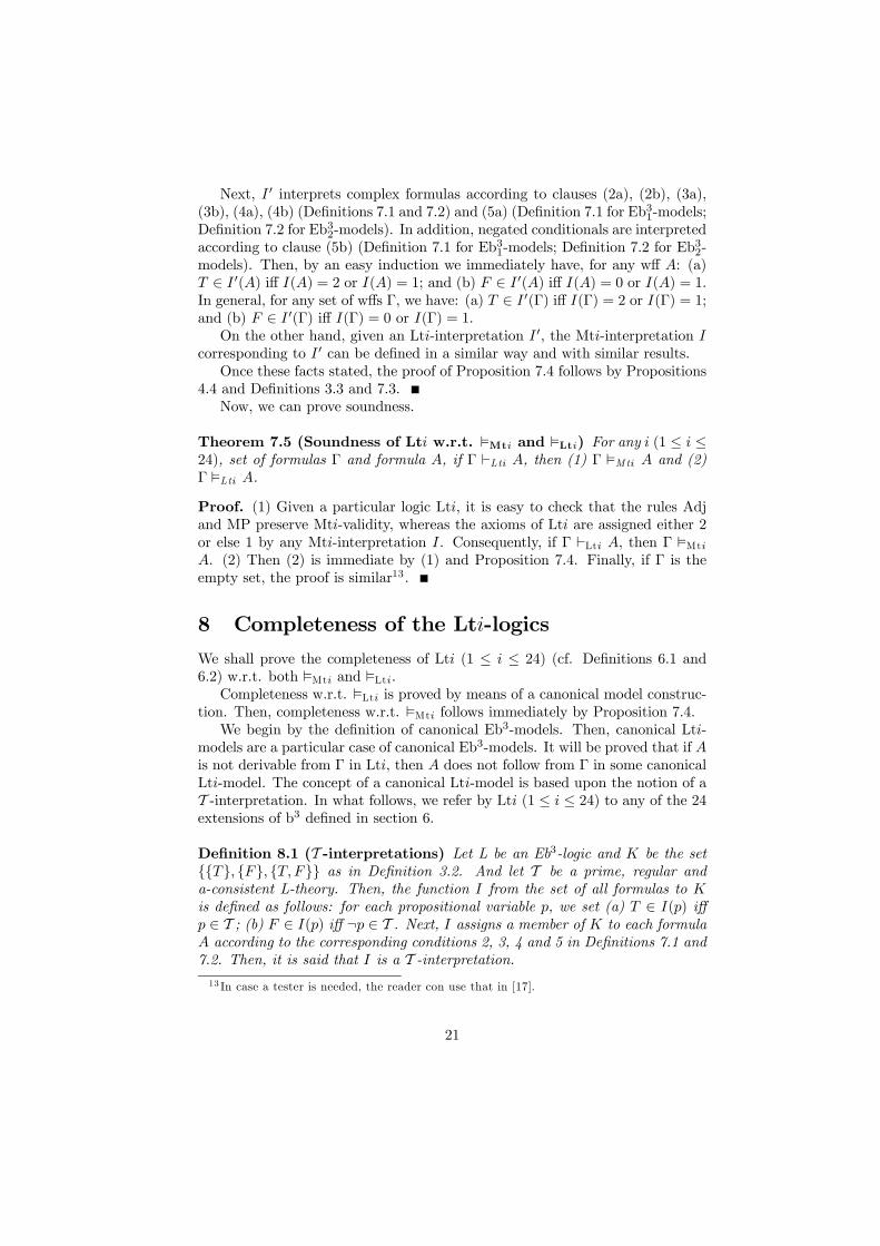
Next, 0 interprets complex formulas according to clauses (2a), (2b), (3a),(3b), (4a), (4b) (Definitions 7.1 and 7.2) and (5a) (Definition 7.1 for Eb31-models;

Definition 7.2 for Eb32-models). In addition, negated conditionals are interpreted

according to clause (5b) (Definition 7.1 for Eb31-models; Definition 7.2 for Eb32-

models). Then, by an easy induction we immediately have, for any wff : (a)

∈ 0() iff () = 2 or () = 1; and (b) ∈ 0() iff () = 0 or () = 1.In general, for any set of wffs Γ, we have: (a) ∈ 0(Γ) iff (Γ) = 2 or (Γ) = 1;and (b) ∈ 0(Γ) iff (Γ) = 0 or (Γ) = 1.On the other hand, given an Lt-interpretation 0, the Mt-interpretation

corresponding to 0 can be defined in a similar way and with similar results.Once these facts stated, the proof of Proposition 7.4 follows by Propositions

4.4 and Definitions 3.3 and 7.3.

Now, we can prove soundness.

Theorem 7.5 (Soundness of Lt w.r.t. ²Mt and ²Lt) For any (1 ≤ ≤24), set of formulas Γ and formula , if Γ `Lt , then (1) Γ ²Mt and (2)

Γ ²Lt .

Proof. (1) Given a particular logic Lt, it is easy to check that the rules Adj

and MP preserve Mt-validity, whereas the axioms of Lt are assigned either 2or else 1 by any Mt-interpretation . Consequently, if Γ `Lt , then Γ ²Mt. (2) Then (2) is immediate by (1) and Proposition 7.4. Finally, if Γ is theempty set, the proof is similar13 .

8 Completeness of the Lt-logics

We shall prove the completeness of Lt (1 ≤ ≤ 24) (cf. Definitions 6.1 and6.2) w.r.t. both ²Mt and ²Lt.Completeness w.r.t. ²Lt is proved by means of a canonical model construc-

tion. Then, completeness w.r.t. ²Mt follows immediately by Proposition 7.4.We begin by the definition of canonical Eb3-models. Then, canonical Lt-

models are a particular case of canonical Eb3-models. It will be proved that if

is not derivable from Γ in Lt, then does not follow from Γ in some canonicalLt-model. The concept of a canonical Lt-model is based upon the notion of a

T -interpretation. In what follows, we refer by Lt (1 ≤ ≤ 24) to any of the 24extensions of b3 defined in section 6.

Definition 8.1 (T -interpretations) Let L be an Eb3-logic and be the set

{{} {} { }} as in Definition 3.2. And let T be a prime, regular and

a-consistent L-theory. Then, the function from the set of all formulas to

is defined as follows: for each propositional variable , we set (a) ∈ () iff ∈ T ; (b) ∈ () iff ¬ ∈ T . Next, assigns a member of to each formula

according to the corresponding conditions 2, 3, 4 and 5 in Definitions 7.1 and

7.2. Then, it is said that is a T -interpretation.13 In case a tester is needed, the reader con use that in [17].

21

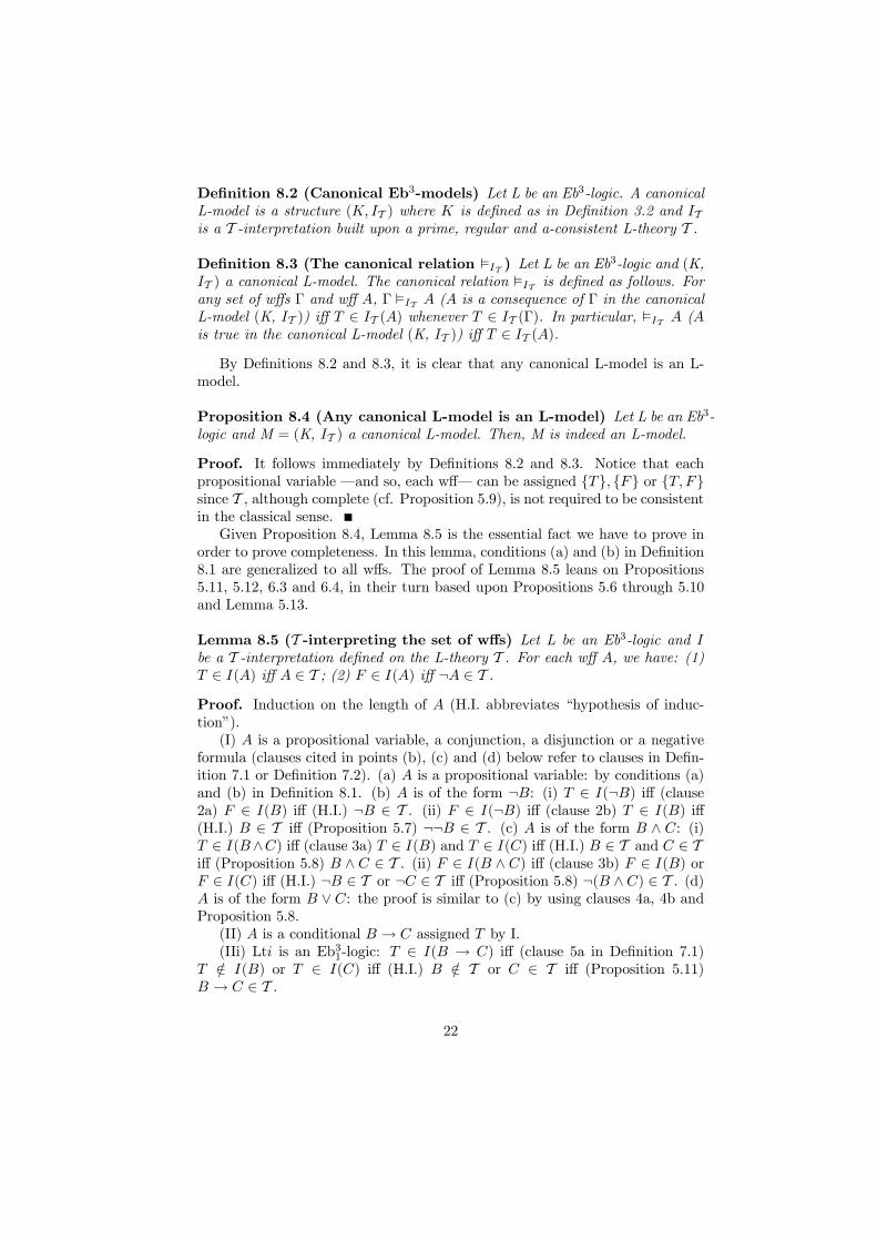
Definition 8.2 (Canonical Eb3-models) Let L be an Eb3-logic. A canonical

L-model is a structure ( T ) where is defined as in Definition 3.2 and Tis a T -interpretation built upon a prime, regular and a-consistent L-theory T .

Definition 8.3 (The canonical relation ²T ) Let L be an Eb3-logic and (K,T ) a canonical L-model. The canonical relation ²T is defined as follows. Forany set of wffs Γ and wff , Γ ²T ( is a consequence of Γ in the canonicalL-model (K, T )) iff ∈ T () whenever ∈ T (Γ). In particular, ²T (

is true in the canonical L-model (K, T )) iff ∈ T ().

By Definitions 8.2 and 8.3, it is clear that any canonical L-model is an L-

model.

Proposition 8.4 (Any canonical L-model is an L-model) Let L be an Eb3-

logic and M = (K, T ) a canonical L-model. Then, M is indeed an L-model.

Proof. It follows immediately by Definitions 8.2 and 8.3. Notice that each

propositional variable –and so, each wff– can be assigned {} {} or { }since T , although complete (cf. Proposition 5.9), is not required to be consistentin the classical sense.

Given Proposition 8.4, Lemma 8.5 is the essential fact we have to prove in

order to prove completeness. In this lemma, conditions (a) and (b) in Definition

8.1 are generalized to all wffs. The proof of Lemma 8.5 leans on Propositions

5.11, 5.12, 6.3 and 6.4, in their turn based upon Propositions 5.6 through 5.10

and Lemma 5.13.

Lemma 8.5 (T -interpreting the set of wffs) Let L be an Eb3-logic and

be a T -interpretation defined on the L-theory T . For each wff , we have: (1)

∈ () iff ∈ T ; (2) ∈ () iff ¬ ∈ T .Proof. Induction on the length of (H.I. abbreviates “hypothesis of induc-

tion”).

(I) is a propositional variable, a conjunction, a disjunction or a negative

formula (clauses cited in points (b), (c) and (d) below refer to clauses in Defin-

ition 7.1 or Definition 7.2). (a) is a propositional variable: by conditions (a)

and (b) in Definition 8.1. (b) is of the form ¬: (i) ∈ (¬) iff (clause2a) ∈ () iff (H.I.) ¬ ∈ T . (ii) ∈ (¬) iff (clause 2b) ∈ () iff(H.I.) ∈ T iff (Proposition 5.7) ¬¬ ∈ T . (c) is of the form ∧ : (i) ∈ (∧) iff (clause 3a) ∈ () and ∈ () iff (H.I.) ∈ T and ∈ Tiff (Proposition 5.8) ∧ ∈ T . (ii) ∈ ( ∧ ) iff (clause 3b) ∈ () or ∈ () iff (H.I.) ¬ ∈ T or ¬ ∈ T iff (Proposition 5.8) ¬( ∧ ) ∈ T . (d) is of the form ∨ : the proof is similar to (c) by using clauses 4a, 4b andProposition 5.8.

(II) is a conditional → assigned by I.

(IIi) Lt is an Eb31-logic: ∈ ( → ) iff (clause 5a in Definition 7.1) ∈ () or ∈ () iff (H.I.) ∈ T or ∈ T iff (Proposition 5.11)

→ ∈ T .

22

(IIii) Lt is an Eb32-logic: ∈ ( → ) iff (clause 5a in Definition 7.2)[ ∈ () or ∈ ()] or [ ∈ () and ∈ ()] iff (H.I.) [ ∈ T or

¬ ∈ T ] or [¬ ∈ T and ∈ T ] iff (Proposition 5.12) → ∈ T .(III) is a conditional → assigned by . We have to consider 24

different cases, but we think that a couple of examples will be sufficient.

(IIIi) Lt is an Eb31-logic: Let Lt be, say, Lt12. We have ∈ ( → )iff (clause 5b in Definition 7.1) [ ∈ () and ∈ ()] or [ ∈ () and ∈ () and ∈ ()] iff (H.I.) [ ∈ T and ∈ T ] or [ ∈ T and ¬ ∈ Tand ∈ T ] iff (Proposition 6.3) ¬( → ) ∈ T .(IIIii) Lt is an Eb32-logic: Let Lt be, for instance, Lt22. We have ∈ ( →

) iff (clause 5b in Definition 7.2) [ ∈ () and ∈ ()] or [ ∈ () and ∈ ()] iff (H.I.) [ ∈ T and ∈ T ] or [¬ ∈ T and ¬ ∈ T ] iff (Proposition6.4) ¬( → ) ∈ T .Next, we recall the notion of set of consequences of a given set of formulas

Γ in Lt and then we prove completeness.

Definition 8.6 (The set of consequences of Γ in Lt) The set of consequen-ces in Lt of a set of wffs Γ (in symbols CnΓ[Lt]) is defined as follows: CnΓ[Lt] ={ | Γ `Lt }.We note the following remark.

Remark 8.7 (The set of consequences of Γ in Lt is a regular theory)It is obvious that for any Γ, CnΓ[Lt] is closed under Adj and MP and containsall theorems of Lt. Consequently, it is closed under Lt-entailment.

Theorem 8.8 (Completeness of Lt-logics) For any (1 ≤ ≤ 24), set offormulas Γ and formula , (1) if Γ ²Lt , then Γ `Lt ; (2) if Γ ²Mt , thenΓ `Lt .Proof. (1) Suppose there are set of wffs Γ and wff such that Γ 0Lt . Weprove Γ 2Lt . If Γ 0Lt , clearly ∈ CnΓ[Lt]. Then, by the PrimenessLemma (Lemma 5.13), there is a prime Lt-theory T such that Γ ⊆ T [Γ ⊆CnΓ[Lt] ⊆ T ] and ∈ T . Thus T is regular (by Remark 8.7) and a-consistent(since ∈ T ). Then, T generates a T -interpretation T such that ∈ T (Γ)but ∈ T () (cf. Lemma 8.5). Consequently, Γ 2T (cf. Definition 8.3 and

Proposition 8.4) and, finally, Γ 2Lt , by Definition 7.3, QED. (2) Completenessw.r.t. ²Mt is immediate by (1) and Proposition 7.4.If Γ is the empty set, let Lt be the set of all theorems of Lt. Then Lt 0Lt

and we can proceed similarly as in cases (1) and (2) above.

9 Concluding remarks

The paper is ended with some remarks.

23

1. Most of the Lt-logics defined above had not been brought to light before

(to the best of our knowledge). However, there is a couple of famous 3-

valued logics among them. Lt16 is the logic RM3, the 3-valued extension

of the quasi-relevant logic RM (cf. [11]); and Lt17 is the logic Pac (which

abbreviates “paraconsistency”, firstly defined by Asenjo in 1954 (cf. [4],

[5], [24], [25]).

2. Given the axiomatizations provided in Definitions 6.1 and 6.2, it is pos-

sible to define all Lt-logics more conspicuously and economically than in

Definitions 6.1 and 6.2. For instance, consider Example 9.1 where Lt22

and Lt23 are defined as negation expansions of the positive fragment of

Lewis’ S4 (cf. [18]) and positive intuitionistic logic, respectively.

Example 9.1 Lt22

Axioms: (a1) → ; (a2) ( ∧ ) → / ( ∧ ) → ; (a3) [( →) ∧ ( → )] → [ → ( ∧ )]; (a4) → ( ∨ ) / → ( ∨ );(a5) [( → ) ∧ ( → )] → [( ∨ ) → ]; (a6) [ ∧ ( ∨ )] →[( ∧ ) ∨ ( ∧ )]; (a7) [ → ( → )] → [( → ) → ( → )];(a8) ( → ) → [ → ( → )]; (a9) ( → ¬) → ( → ¬); (a10)(¬ → ) → (¬ → ); (a11) ∨ ¬; (a12) (¬ ∧ ) → ( → );(a13) ¬→ [ ∨ (→ )]; (a14) [¬(→ ) ∧ (¬ ∧)]→ .

Rules of inference: (Modus Ponens) → & ⇒ ; (Adjunction)

& ⇒ ∧.Lt23

Axioms: a1-a7 of Lt22 plus (a8) → ( → ); (a9) → ¬¬; (a10)¬¬ → ; (a11) ∨ ¬; (a12) → [ ∨ ¬( → )]; (a13) ¬ →[¬ ∨ ¬( → )]; (a14) ¬( → ) → ( ∧ ¬); (a15) [¬( → ) ∧(¬ ∧)]→ .

Rules: MP and Adj.

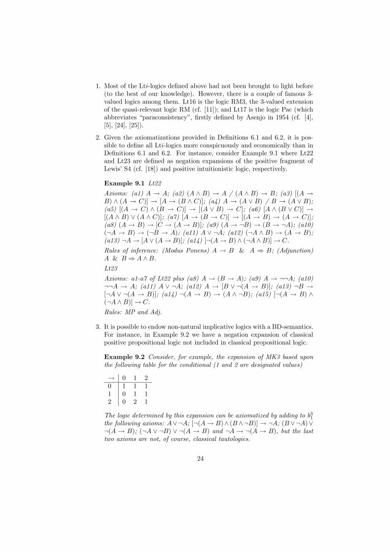
3. It is possible to endow non-natural implicative logics with a BD-semantics.

For instance, in Example 9.2 we have a negation expansion of classical

positive propositional logic not included in classical propositional logic.

Example 9.2 Consider, for example, the expansion of MK3 based upon

the following table for the conditional (1 and 2 are designated values)

→ 0 1 20 1 1 11 0 1 12 0 2 1

The logic determined by this expansion can be axiomatized by adding to b31the following axioms: ∨¬; [¬(→ )∧ (∧¬)]→ ¬; ( ∨¬)∨¬( → ); (¬ ∨ ¬) ∨ ¬( → ) and ¬ → ¬( → ), but the lasttwo axioms are not, of course, classical tautologies.

24

4. All Eb31-logics contain classical positive propositional logic but lack the

rule Contraposition (if → , then ¬ → ¬); in their turn, all Eb32-logics, except Lt16 and Lt22, lack the rule Prefixing (if → , then

(→ )→ ( → )) or the rule Suffixing (if → , then ( → )→(→ )) (Lt1, Lt4, Lt7 and Lt10 lack Prefixing and Lt13 and Lt19 lackSuffixing). Consequently, Sylvan and Plumwood’s minimal logic BM (cf.

[32]) is not contained in any of the Lt-logics, except Lt16 and Lt22.

5. All Lt-logics are paraconsistent in the sense that the rule ECQ (if ∧¬,then ) does not hold in any of them (cf. [26], [27]).

6. A referee of the JANCL called out our attention to some work related

to the research recorded in our paper. In particular, Kooi and Tamminga

[21] study truth-functional extensions of LP (cf. [24] and [25]) in a natural

deduction setting, whereas Petrukhin and Shangin [23] investigate some

implicational extensions of LP, including extensions by natural implica-

tions in the sense of Tomova [34]. Also, Thomas [33] has to be mentioned.

In this paper, an extension of LP with Rescher’s implication is proposed.

Future work on the topic of the present paper could consist in the study

of the relations the papers mentioned maintain to each other.

Acknowledgements. - This work is supported by the Spanish Ministry of

Economy, Industry and Competitiveness under Grants [FFI2014-53919-P; FFI2017-

82878-P]. - We sincerely thank two referees of the JANCL for their comments

and suggestions on a previous version of this paper.

References

[1] Anderson, A. R., Belnap, N. D. J. (1975). Entailment. The Logic of Rele-

vance and Necessity, vol I. Princeton, NJ: Princeton University Press.

[2] Arieli, O., Avron, A. (1996). Reasoning with logical bilattices. Journal of

Logic, Language and Information, 5(1), 25-63.

[3] Arieli, O., Avron, A. (1998). The value of the four values. Artificial Intel-

ligence, 102, 97-141.

[4] Asenjo, F. G. (1954). La Idea de un Cálculo de Antinomias. Seminario

Matemático. Universidad Nacional de la Plata.

[5] Asenjo, F. G. (1966). A calculus of antinomies. Notre Dame Journal of

Formal Logic, 7(1), 103—105. http://doi.org/10.1305/ndjfl/1093958482.

[6] Avron, A. (1986). On an implicational connective of RM. Notre Dame

Journal of Formal Logic, 27(2), 201-209.

[7] Avron, A. (1991). Natural 3-Valued Logics—Characterization and Proof

Theory. Journal of Symbolic Logic, 56(1), 276-294.

25

[8] Belnap, N. D. Jr. (1960). Entailment and relevance. The Journal of Sym-

bolic Logic, 25(2), 144-146.

[9] Belnap, N. D. Jr. (1977a). A useful four-valued logic. In G. Epstein, J. M.

Dunn (Eds.), Modern Uses of Multiple-Valued Logic (pp. 8-37). D. Reidel

Publishing Co., Dordrecht.

[10] Belnap, N. D. Jr. (1977b). How a computer should think. In G. Ryle (Ed.),

Contemporary Aspects of Philosophy (pp. 30-55). Oriel Press Ltd., Stocks-

field.

[11] Brady, R. T. (1982). Completeness Proofs for the Systems RM3 and BN4.

Logique et Analyse, 25, 9-32.

[12] Carnielli, W., Marcos, J., Amo, S. de. (2000). Formal inconsistency

and evolutionary databases. Logic and Logical Philosophy, 8, 115-152.

https://doi.org/10.12775/LLP.2000.008

[13] Ciucci, D., Dubois, D. (2014). Three-Valued Logics, Uncertainty Manage-

ment and Rough Sets. In J. F. Peters, A. Skowron (Eds.), Transactions on

Rough Sets XVII. Lecture Notes in Computer Science, vol 8375 (pp. 1-32).

Springer, Berlin, Heidelberg.

[14] Dunn, J. M. (1976). Intuitive semantics for first-degree entailments and

“coupled trees.” Philosophical Studies, 29, 149-168.

[15] Dunn, J. M. (2000). Partiality and its Dual. Studia Logica, 66(1), 5-40.

http://doi.org/10.1023/A:1026740726955.

[16] Gaines, B. R. (1976). Foundations of fuzzy reasoning. International Jour-

nal of Man-Machine Studies, 8(6), 623-668. https://doi.org/10.1016/S0020-

7373(76)80027-2

[17] González, C. (2012). MaTest. Retrieved from http://ceguel.es/matest (last

accessed 04/01/2018).

[18] Hacking, I. (1963). What is Strict Implication? Journal of Symbolic Logic,

28(1), 51-71.

[19] Karpenko, A. S. (2004). Jaskowski’s criterion and three-valued

paraconsistent logics. Logic and Logical Philosophy, 7, 81—86.

https://doi.org/10.12775/LLP.1999.006

[20] Kleene, S. C. (1962). Introduction to Metamathematics. North Holland.

Reprinted Ishi Press, 2009.

[21] Kooi, B., Tamminga, A. (2012). Completeness via correspondece for exten-

sions of the logic of paradox. The Review of Symbolic Logic, 5(4), 720-730.

26

[22] Méndez, J. M., Robles, G. (2016). The logic determined by

Smiley’s matrix for Anderson and Belnap’s First Degree Entail-

ment Logic. Journal of Applied Non-Classical Logics, 26(1), 47-68.

http://doi.org/10.1080/11663081.2016.1153930.

[23] Petrukhin, Y., Shangin, V. (2017). Automated correspondence analysis for

the binary extensions of the logic of paradox. The Review of Symbolic Logic,

10(4), 756-781. https://doi.org/10.1017/S1755020317000156.

[24] Priest, G. (1979). Logic of Paradox. Journal of Philosophical Logic, 8 (1),

219-241.

[25] Priest, G. (1984). Logic of paradox revisited. Journal of Philosophical Logic,

13(2), 153-179. https://doi.org/10.1007/BF00453020.

[26] Priest, G. (2002). Paraconsistent Logic. In D. M. Gabbay, F. Guenthner

(Eds.), Handbook of Philosophical Logic vol. 6 (pp. 287-393). Springer, Dor-

drecht.

[27] Priest, G., Tanaka, K. and Weber, Z. (2017). Paraconsistent Logic. The

Stanford Encyclopedia of Philosophy (Fall 2017 Edition), E. N. Zalta (Ed.),

URL = https://plato.stanford.edu/archives/fall2017/

entries/logic-paraconsistent/.

[28] Robles, G. (2014). A simple Henkin-style completeness proof for

Gödel 3-valued logic G3. Logic and Logical Philosophy, 23(4), 371-390.

http://doi.org/10.12775/LLP.2014.001.

[29] Robles, G., Méndez, J. M. (2014). A paraconsistent 3-valued logic re-

lated to Gödel logic G3. Logic Journal of the IGPL, 22(4), 515-538.

http://doi.org/10.1093/jigpal/jzt046.

[30] Robles, G., Méndez, J. M. (In preparation). Belnap-Dunn semantics for

natural implicative expansions of Kleene’s strong three-valued matrix II.

Only one designated value.

[31] Robles, G., Salto, F., Méndez, J. M. (2014). Dual Equivalent Two-valued

Under-determined and Over-determined Interpretations for Łukasiewicz’s

3-valued Logic Ł3. Journal of Philosophical Logic, 43(2/3), 303-332.

http://doi.org/10.1007/s10992-012-9264-0.

[32] Sylvan, R., Plumwood, V. (2003). Non-normal relevant logics. In R. Brady

(Ed.), Relevant logics and their rivals, vol. II (pp. 10-16). Ashgate, Alder-

shot and Burlington: Western Philosophy Series.

[33] Thomas, N. (2018), LP⇒: Extending LP with a strong conditional opera-tor. Cornell University Library. Unpublished manuscript.

[34] Tomova, N. (2012). A Lattice of implicative extensions of regu-

lar Kleene’s logics. Reports on Mathematical Logic, 47, 173-182.

http://doi.org/10.4467/20842589RM.12.008.0689.

27