Bellwether Analysis: Predicting Global Aggregates from Local Regions

Bee-Chung Chen1, Raghu Ramakrishnan

1,2, Jude W. Shavlik

1, Pradeep Tamma

1

1 University of Wisconsin – Madison, USA

2 Yahoo! Research, Santa Clara, CA, USA

{beechung, shavlik, pradeep}@cs.wisc.edu ramakris@yahoo-inc.com

ABSTRACT

Massive datasets are becoming commonplace in a wide range of

domains, and mining them is recognized as a challenging problem

with great potential value. Motivated by this challenge, much

effort has been concentrated on developing scalable versions of

machine learning algorithms. An often overlooked issue is that

large datasets are rarely labeled with the outputs that we wish to

learn to predict, due to the human labor required. We make the

key observation that analysts can often use queries to define labels

for cases, which leads to the problem of learning to predict such

query-produced labels. Of course, if a dataset is available in its

entirety, we can simply run the query again to compute labels. The

interesting scenarios are those where, after the predictive model is

trained, new data is gathered at significant incremental cost and,

perhaps, over time. The challenge is to accurately predict the

query-labels for the projected completion of new datasets, based

only on certain cost-effective subsets, which we call bellwethers.

1. INTRODUCTION Mining large datasets is recognized as a challenging problem with great potential value, and much effort has been concentrated on developing scalable versions of machine learning algorithms. However, large datasets are rarely labeled with the outputs that we wish to learn to predict, due to the human labor that is typically required. This severely limits our ability to apply supervised learning techniques.

We make the key observation that for a large class of practically motivated problems, conventional database queries can be used to “tag” cases with the attribute values that we wish to predict, thereby mitigating the labeling difficulty. The “cases” are themselves the result of aggregating many database records. Consider a company that wants to predict the 1st year worldwide profit of a new item. After selling this item worldwide for one year, the company will know the exact profit. However, if the company can accurately predict the annual worldwide profit using features (e.g., regional profit, etc.) collected in a much shorter time (e.g., 1st week sales) and a much smaller area (e.g., only sales in Wisconsin), it has gained valuable business insight.

In this example, each item for which we have historical data is a case, and the information relating to this item is dispersed across

all sales records for the item. We can create additional per-item features, and compute the desired label (worldwide annual profit for the item), by using conventional OLAP-style queries. In fact we can create training datasets by summarizing historical per-item sales for each region of interest (e.g., by state and month, or by county and week). We can then use each per-region training dataset to train a predictive data model. When a new item is introduced, if we collect sales data for a given region and aggregate this as before to create a case for the new item, the predictive model for the region can be used to estimate the desired label, which, in our example, is worldwide annual profit.

The question, then, is what is the best region on which to base such a predictive model, and whether a good region exists at all. Intuitively, gathering sales data for a new item in the region must be within an acceptable cost; cost could reflect real-world marketing expenses, for example. Further, the predictive model for the region must have high accuracy and low variance. We call such regions bellwethers, and the problem considered in this paper is how to identify bellwether regions.

In this paper, we make the following contributions: (1) We introduce bellwether analysis, a novel framework that allows us to apply predictive models to massive datasets without human labor for labeling the training examples. (2) We formalize many challenges raised by this framework, showing the richness of the problem and many opportunities for future research. (3) We develop several efficient, scalable algorithms to find bellwether regions, and evaluate their performance. (4) Using real-life datasets, we demonstrate the value of bellwether analysis.

The rest of this paper is organized as follows. After reviewing predictive models in Section 2, we introduce bellwether analysis in Section 3. We define the basic bellwether analysis problem, and an important variation, finding item-centric bellwethers. Intuitively, the basic approach finds a single region to serve as bellwether for all items, while the latter recognizes that different regions may be appropriate for different items or types of items. We present a scalable algorithm for basic bellwether analysis in Section 4, and two algorithms for item-centric bellwethers in Sections 5 and 6. In Section 7, we present a detailed experimental evaluation using both real and synthetic datasets, measuring both the quality of the bellwethers found and the efficiency of our algorithms. We discuss related work and conclude in Section 8.

2. BACKGROUND Before formally introducing bellwether analysis, we first review some basics of predictive models [13]. Let D be a data table with attributes X1, …, Xp, Y, where X1, …, Xp are called features, Y is called the target, and each row in the table is called an example. A predictive model learns the relationship between X1, …, Xp and Y from D and predicts the value of Y given a new example based on its X1, …, Xp values. D is called the training set. We use h to denote a predictive model, and h(x) returns the target value of example x. If the target Y is a numeric value, h is called a

Permission to copy without fee all or part of this material is granted

provided that the copies are not made or distributed for direct commercial

advantage, the VLDB copyright notice and the title of the publication and

its date appear, and notice is given that copying is by permission of the

Very Large Data Base Endowment. To copy otherwise, or to republish, to

post on servers or to redistribute to lists, requires a fee and/or special

permission from the publisher, ACM.

VLDB ‘06, September 12–15, 2006, Seoul, Korea.

Copyright 2006 VLDB Endowment, ACM 1-59593-385-9/06/09

regression model. If Y is a categorical value, h is called a classification model. Decision trees, support vector machines, neural networks and linear regression models are examples of predictive models.

The quality of a predictive model is usually measured by the error (or equivalently, accuracy) of the model, which is the expected discrepancy between the true target value and the predicted value for a new example. For classification models, the misclassification rate (i.e., the expectation of making an incorrect prediction) is a commonly used error measure, while for regression models, the mean squared error (MSE) and root mean squared error (RMSE) are commonly used. MSE is the expected value of the squared difference between the true Y value and the predicted one, and RMSE is the square root of MSE. However, in reality, the true distribution of X1, …, Xp, Y is generally unknown. Thus, the error of a model cannot be computed exactly, but needs to be estimated from the given data D. We consider two commonly used error estimates: cross-validation error and training-set error.

Cross-validation error: To compute cross-validation error, we first partition D into n non-overlapping subsets of examples: D1, …, Dn. For i from 1 to n, we train a model on ∪j≠i Dj and test the model on Di to obtain an error value. Then, the cross-validation error is the mean of the n error values. Based on some distribution assumptions, the confidence interval of the cross-validation error can be obtained based on the variance of the n error values. A commonly used n is 10.

Training-set error: Another way to estimate the error of a model is to train the model on D, and then test it also on D to obtain the error value, which is called the training-set error. Usually training-set error is overly optimistic. However, for simple models, e.g., linear regression models, training-set error can approximate the true error. Note that the overhead of computing cross-validation error is approximately n times that of computing training-set error.

3. PROBLEM DEFINITION We first introduce a motivating example, and then formally define the problem of bellwether analysis. Intuitively, we want to use historical data to find a region (e.g., [1st week, Wisconsin]) with a small cost such that we can accurately predict the target value (e.g., the 1st year worldwide sales) of an item (e.g., a product) based on the features (e.g., the 1st week sales in Wisconsin) of that item collected from that region. As will be seen, this problem is significantly different from ordinary machine-learning problems in that both features and target values are generated by queries over the historical database.

3.1 Motivating Example Consider a company that wants to predict the 1st year worldwide profit of a new item. After selling this item worldwide for one year, the company will know the exact profit. However, if the company can accurately predict this target value using features

(e.g., regional profit, etc.) collected in a much shorter time (e.g., 1st week) and a much smaller area (e.g., only focus on Wisconsin), then it can quickly adapt its business strategy to minimize the loss or even maximize the profit. [1st week, Wisconsin] is an example of such a bellwether region. Our goal is to find such regions. Note that, in this example, we denote a region by a pair of time interval and location values.

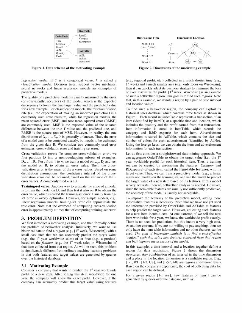
To find such a bellwether region, the company can exploit its historical sales database, which contains three tables as shown in Figure 1. Each record in OrderTable represents a transaction of an item (identified by ItemID) at a specific time and location, which includes the quantity and the profit earned from that transaction. Item information is stored in ItemTable, which records the category and R&D expense for each item. Advertisement information is stored in AdTable, which contains the size and number of colors for each advertisement (identified by AdNo). Using the foreign keys, we can obtain the item and advertisement information for each transaction.

Let us first consider a straightforward data-mining approach. We can aggregate OrderTable to obtain the target value (i.e., the 1st year worldwide profit) for each historical item. Thus, a training set can be created by associating the features (Category and RDexpense) of each item, called the item-table features, with its target value. Then, we can train a predictive model (e.g., a linear regression model) on the training set, and use the model to predict the target value of a new item based on its features. If this model is very accurate, then no bellwether analysis is needed. However, since the item-table features are usually not sufficiently predictive, the accuracy of the model is usually not acceptable.

To improve the accuracy of the predictive model, adding more informative features is necessary. Note that we have not yet used the information provided by OrderTable and AdTable as features to help predict the target value. However, collecting such features for a new item incurs a cost. At one extreme, if we sell the new item worldwide for a year, we know the worldwide profit exactly. There is no need for prediction, but this incurs a very high cost. At another extreme, if we are not willing to pay anything, then we only have the item table information and no other features can be used. The goal of bellwether analysis is to find a cost-effective “region,” such that using new features collected from that region can best improve the accuracy of the model.

In this example, a time interval and a location together define a region for data acquisition. Figure 2 shows the dimension structures. Any combination of an interval in the time dimension and a place in the location dimension is a candidate region. E.g., [1-1, WI], [1-2, US], and [1-52, All] are regions at different levels. Based on the company’s experience, the cost of collecting data for each region can be defined.

For a given region [1-t, loc], new features of item i can be generated by queries over the database, such as:

OrderTable

Time

Location

ItemID

AdNo

Quantity

Profit

ItemTable

ItemID

Category

RDExpense

AdTable

AdNo

AdSize

NumColors

All

CA US KR

AL WI

All

Country

State

Dimension: LocationDimension: Time

Week 1-1

Week 1-2

Week 1-52

(i.e., 1st year)

Figure 1. Data schema of the motivating example Figure 2. Dimensions of the motivating example

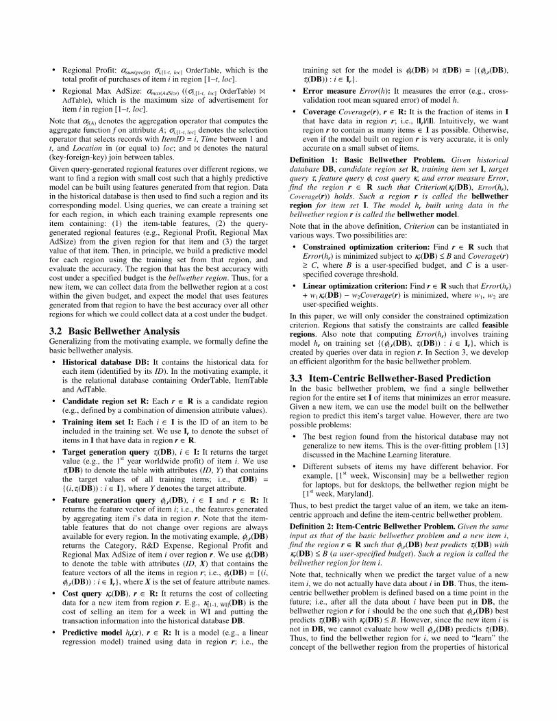
� Regional Profit: αsum(profit) σi,[1-t, loc] OrderTable, which is the total profit of purchases of item i in region [1−t, loc].

� Regional Max AdSize: αmax(AdSize) ((σi,[1-t, loc] OrderTable) ⋈AdTable), which is the maximum size of advertisement for item i in region [1−t, loc].

Note that αf(A) denotes the aggregation operator that computes the aggregate function f on attribute A; σi,[1-t, loc] denotes the selection operator that selects records with ItemID = i, Time between 1 and t, and Location in (or equal to) loc; and ⋈ denotes the natural (key-foreign-key) join between tables.

Given query-generated regional features over different regions, we want to find a region with small cost such that a highly predictive model can be built using features generated from that region. Data in the historical database is then used to find such a region and its corresponding model. Using queries, we can create a training set for each region, in which each training example represents one item containing: (1) the item-table features, (2) the query-generated regional features (e.g., Regional Profit, Regional Max AdSize) from the given region for that item and (3) the target value of that item. Then, in principle, we build a predictive model for each region using the training set from that region, and evaluate the accuracy. The region that has the best accuracy with cost under a specified budget is the bellwether region. Thus, for a new item, we can collect data from the bellwether region at a cost within the given budget, and expect the model that uses features generated from that region to have the best accuracy over all other regions for which we could collect data at a cost under the budget.

3.2 Basic Bellwether Analysis Generalizing from the motivating example, we formally define the basic bellwether analysis.

� Historical database DB: It contains the historical data for each item (identified by its ID). In the motivating example, it is the relational database containing OrderTable, ItemTable and AdTable.

� Candidate region set R: Each r ∈ R is a candidate region (e.g., defined by a combination of dimension attribute values).

� Training item set I: Each i ∈ I is the ID of an item to be included in the training set. We use Ir to denote the subset of items in I that have data in region r ∈ R.

� Target generation query τi(DB), i ∈ I: It returns the target value (e.g., the 1st year worldwide profit) of item i. We use τ(DB) to denote the table with attributes (ID, Y) that contains the target values of all training items; i.e., τ(DB) = {(i,τi(DB)) : i ∈ I}, where Y denotes the target attribute.

� Feature generation query φi,r(DB), i ∈ I and r ∈ R: It returns the feature vector of item i; i.e., the features generated by aggregating item i’s data in region r. Note that the item-table features that do not change over regions are always available for every region. In the motivating example, φi,r(DB) returns the Category, R&D Expense, Regional Profit and Regional Max AdSize of item i over region r. We use φr(DB) to denote the table with attributes (ID, X) that contains the feature vectors of all the items in region r; i.e., φr(DB) = {(i, φi,r(DB)) : i ∈ Ir}, where X is the set of feature attribute names.

� Cost query κr(DB), r ∈ R: It returns the cost of collecting data for a new item from region r. E.g., κ[1-1, WI](DB) is the cost of selling an item for a week in WI and putting the transaction information into the historical database DB.

� Predictive model hr(x), r ∈ R: It is a model (e.g., a linear regression model) trained using data in region r; i.e., the

training set for the model is φr(DB) ⋈ τ(DB) = {(φi,r(DB), τi(DB)) : i ∈ Ir}.

� Error measure Error(h): It measures the error (e.g., cross-validation root mean squared error) of model h.

� Coverage Coverage(r), r ∈ R: It is the fraction of items in I that have data in region r; i.e., |Ir|/|I|. Intuitively, we want region r to contain as many items ∈ I as possible. Otherwise, even if the model built on region r is very accurate, it is only accurate on a small subset of items.

Definition 1: Basic Bellwether Problem. Given historical database DB, candidate region set R, training item set I, target query τ, feature query φ, cost query κ, and error measure Error, find the region r ∈ R such that Criterion(κr(DB), Error(hr), Coverage(r)) holds. Such a region r is called the bellwether region for item set I. The model hr built using data in the bellwether region r is called the bellwether model.

Note that in the above definition, Criterion can be instantiated in various ways. Two possibilities are:

� Constrained optimization criterion: Find r ∈ R such that Error(hr) is minimized subject to κr(DB) ≤ B and Coverage(r) ≥ C, where B is a user-specified budget, and C is a user- specified coverage threshold.

� Linear optimization criterion: Find r ∈ R such that Error(hr) + w1κr(DB) − w2Coverage(r) is minimized, where w1, w2 are user-specified weights.

In this paper, we will only consider the constrained optimization criterion. Regions that satisfy the constraints are called feasible regions. Also note that computing Error(hr) involves training model hr on training set {(φi,r(DB), τi(DB)) : i ∈ Ir}, which is created by queries over data in region r. In Section 3, we develop an efficient algorithm for the basic bellwether problem.

3.3 Item-Centric Bellwether-Based Prediction In the basic bellwether problem, we find a single bellwether region for the entire set I of items that minimizes an error measure. Given a new item, we can use the model built on the bellwether region to predict this item’s target value. However, there are two possible problems:

� The best region found from the historical database may not generalize to new items. This is the over-fitting problem [13] discussed in the Machine Learning literature.

� Different subsets of items my have different behavior. For example, [1st week, Wisconsin] may be a bellwether region for laptops, but for desktops, the bellwether region might be [1st week, Maryland].

Thus, to best predict the target value of an item, we take an item-centric approach and define the item-centric bellwether problem.

Definition 2: Item-Centric Bellwether Problem. Given the same input as that of the basic bellwether problem and a new item i, find the region r ∈ R such that φi,r(DB) best predicts τi(DB) with κr(DB) ≤ B (a user-specified budget). Such a region is called the bellwether region for item i.

Note that, technically when we predict the target value of a new item i, we do not actually have data about i in DB. Thus, the item-centric bellwether problem is defined based on a time point in the future; i.e., after all the data about i have been put in DB, the bellwether region r for i should be the one such that φi,r(DB) best predicts τi(DB) with κr(DB) ≤ B. However, since the new item i is not in DB, we cannot evaluate how well φi,r(DB) predicts τi(DB). Thus, to find the bellwether region for i, we need to “learn” the concept of the bellwether region from the properties of historical

items. In Sections 4 and 5, we present two methods for finding bellwether regions of new items.

3.4 Discussion and Extension The above problem definitions are fairly general. The candidate region set can contain regions of any form (not necessarily combinations of dimension attribute values), and the feature generation, target generation and cost queries can also be arbitrary functions (not necessarily aggregate-select-join SQL queries). Although the efficient algorithms in this paper apply only to the special case mentioned above (which is actually fairly general), we would also like to point out some other cases to show the richness of the problem and the opportunities for future research.

� Combinatorial bellwether analysis: We previously defined bellwether candidates to be regions in R. Now, a candidate c is a combination of regions; i.e., c ⊆ R. Equivalently, we can specify the candidate region set to be 2R. The search space of combinatorial bellwether analysis is extremely flexible and large, which opens the possibility of finding better bellwether region combinations but requires further techniques to efficiently search through the space.

� Multi-instance bellwether analysis: Previously, we defined the feature generation query φi,r(DB) to return a feature vector for item i aggregated over data in region r. Now, φi,r(DB) returns a set of feature vectors in region r for item i without aggregation. Thus, each training example consists of a set of feature vectors and the target value for that set. This setting is non-standard and similar to multi-instance learning [20].

� Relational bellwether analysis: Some relational predictive models [5] do not need to make predictions based on feature vectors. They can use the whole historical relational database to predict the target value of a new item. In this case, φi,r(DB) returns a relational database consisting of the data about item i in region r and the sub-database of DB that is considered “historical” from region r’s point of view.

� Automatic feature generation: In the current formulation, the user needs to specify the feature generation queries. Since the number of possibly useful queries can be huge, it is desirable to have an automatic feature generation framework.

Also note that, although bellwether analysis may look similar to feature selection (which goal is to select predictive features), they are orthogonal problems. In fact, the models used in bellwether analysis can employ feature selection techniques. However, a unique idea of bellwether analysis is that collecting features from a region requires a region-dependent cost. Finding a cost-effective region is important since useful features are usually not cost free.

4. BASIC BELLWETHER ALGORITHM Ideally, if we have unlimited resources, as long as the candidate region set is finite, we can iterate through all the candidate regions, and for each region, issue a query to create a training set and learn a model from that training set, and finally pick the most cost-effective region as the bellwether region. However, in reality, this computation is very expensive, and we need an efficient algorithm. We now consider an interesting instance of the basic bellwether problem and develop an efficient algorithm.

4.1 OLAP-Style Basic Bellwether Search For efficient computation, we structure the space by considering OLAP-style schemas, regions and aggregate queries. The historical database has a star schema; i.e., DB = {F, T1, …, Tn}, where F is the fact table (e.g., OrderTable) and Ti is a reference table (e.g., ItemTable and AdTable). The link between F and Ti is

through a natural (key-foreign-key) join. F has two special kinds of attributes: ID is the attribute containing the item IDs, and Z={Z1, …, Zd} is the set of dimension attributes (e.g., {Time, Location}), each of which has a dimension structure (e.g., Figure 2). We consider two kinds of dimension structures:

� Interval dimension: The values in the dimension are intervals (e.g., week 1-5). The values recorded in F are time points (e.g., week 4). Currently, we only consider incremental intervals (i.e., from time 1 to time t), but in general they can be defined by different kinds of windows.

� Hierarchical dimension: The values in the dimension are organized as a tree. The values recorded in F are at the lowest (i.e., leaf) level (e.g., State level) of the tree.

Each combination of dimension attribute values defines a candidate region (e.g., R = {[1-1, AL], …, [1-52, All]}). The target generation query τi(DB) can be arbitrary since the target values do not change over different regions and need to be generated only once. The feature generation query φi,r(DB) consists of a set of stylized aggregate-select-join SQL queries, each for an element of the feature vector. The forms of the stylized queries are as follows (Table 1 summarizes the operators we consider):

� αf(F.A) σID=i, Z∈r F: It returns an aggregate value f(F.A) (e.g., sum, min, max or average) of attribute A of table F for item i over region r. E.g., αsum(profit) σ ID=i, Z∈r OrderTable returns the total profit of item i in region r.

� αf(T.A) ((σID=i, Z∈r F) ⋈ T): It returns an aggregate value of attribute A of table T for item i over region r. E.g., αmax(AdSize)

((σID=i, Z∈r OrderTable) ⋈ AdTable) returns the largest size of advertisement for item i in region r.

� αf(T.A) ((πFK σID=i, Z∈r F) ⋈ T), where FK is the foreign key in F that links to the primary key of T: It returns an aggregate value f(T.A) of attribute A of table T for item i over region r. The projection onto FK ensures that each matching row of T is considered only once in the aggregate, even if it matches multiple F tuples. E.g., αsum(AdSize) ((αAdNo σID=i, Z∈r OrderTable) ⋈ AdTable) returns the total size of advertisements used for item i in region r, where each individual advertisement is counted once.

For the cost query κr(DB), we assume the user provides a cost table C with attributes (Z, Cost) describing the cost of each finest-grained region. The cost of a larger region r is αf(Cost) σ Z∈r C, e.g., the sum of costs of all the finest-grained regions in r. Finally, note again that we only consider the constrained optimization criterion.

4.2 An Efficient Algorithm The basic ideas of the algorithm are: (1) we can prune regions with cost > B and coverage < C, so that no model is built for those infeasible regions; and (2) we can generate the training sets for the feasible regions all together, so that data cube computation

Table 1. Operators of extended relational algebra

σID=i, Z∈r F Select all the tuples t in F such that t[ID] = i and t[Z] in region r.

αG, f(A) F Aggregate over F group by G and for each group compute aggregate function f(A). If G is omitted, α aggregates all of F.

πZ F Project F onto a set Z of attributes without duplicates.

F ⋈ T Natural (key-foreign-key) join between tables.

techniques can be applied. In fact, the generation of the training sets for all the feasible regions can be written as a single OLAP query and optimized.

First, we rewrite the three forms of feature generation queries into the following equivalent forms:

� αf(F.A) σID=i, Z∈r F → σ Z=r,ID=i, αZ,ID,f(F.A) F

� αf(T.A) ((σID=i, Z∈r F) ⋈ T) → σZ=r,ID=i αZ,ID,f(T.A) (F ⋈ T)

� αf(T.A) ((πFK σID=i, Z∈r F) ⋈ T) →

σZ=r,ID=i α Z,ID,f(T.A) ((πFK F) ⋈ T)

Note that here we assume the aggregate operator performs the CUBE operation [7] on the dimension attributes; i.e., αZ,ID,f(F.A) F returns a relation containing an aggregate value of f(F.A) for each region (identified by attribute Z) and item (identified by attribute ID). Thus, the selection condition in the rewritten forms becomes Z = r, rather than Z ∈ r. If we remove the selection, each query actually returns a table containing a feature for each region and item. By joining these tables on ID and Z, we obtain all feature vectors of all the items in all the regions. Then, by joining the resulting table with τ(DB) (the table containing the target value for each item) on ID, we associate each feature vector with the target value.

The cost constraint and coverage constraint can also be expressed in OLAP queries. πZ σsum(Cost)≤B αZ,sum(Cost) C returns the regions with cost ≤ B. πZ σcount(ID)≥C* αZ,count(ID) (F ⋈ I) returns all the regions with coverage ≥ C, where count(ID) counts for distinct ID values, I is a table with a single attribute ID specifying the set of items of interest, and C* = C⋅|I| is a constant.

Putting everything together, if the feature vector of item i in region r is ⟨ αf1(F.A) σID=i,Z∈r F, αf2(T.A) ((σID=i,Z∈r F) ⋈ T), αf3(T.A) ((πFK σID=i,Z∈r F) ⋈ T) ⟩. The query to generate all the training sets is as follows:

τ(DB) ⋈ (αZ,ID,f1(F.A) F) ⋈ (αZ,ID,f2(T.A) (F ⋈ T)) ⋈ (α Z,ID,f3(T.A) ((πFK F) ⋈ T)) ⋈

(πZ σsum(Cost)≤B αZ,sum(Cost) C) ⋈ (πZ σcount(ID)≥C* αZ,count(ID) (F ⋈ I))

To efficiently evaluate this query, we can first use iceberg cube techniques [1, 9] to find all the regions satisfying the constraints, and then apply techniques for simultaneously computing multiple aggregate functions [3]. The details are omitted for lack of space.

After generating the training sets for all the feasible regions, we simply build a model for each feasible region and evaluate the error of that model. Then, the region having the minimum-error model is the bellwether region.

5. BELLWETHER TREE Now, we consider the item-centric bellwether-based prediction. The basic idea is that to find the bellwether region for a new item, we first identify a subset S ⊆ I of historical items similar to the new one, and find the bellwether region for S. In this section, we introduce the bellwether tree, where items having different characteristics are recursively partitioned based on item-table features. In the next section, the bellwether cube is introduced, which uses predefined item hierarchies to group similar items.

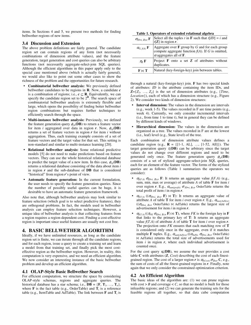
A bellwether tree is similar to a decision/regression tree. Each node in the tree has a splitting criterion (e.g., RDexpense ≥ 50K) that partitions a set of items into several parts. However, at the leaf node, unlike a decision/regression tree that predicts the target value directly based on the items in that leaf, we find the bellwether region for the set of items in that leaf and use that region to serve as the bellwether region for any new item that would be sent to that leaf. Figure 3 shows an example bellwether

tree, where for items with RDexpense ≥ 50K, [1-1, NY] is the bellwether region, while the bellwether region for an item with RDexpense < 50K depends on what category the item belongs to.

The features used in the splitting criteria are the item-table features, which do not depend on regions and are known at the time when we want to predict the target value for any item. Thus, we redefine the item set I to be a table (e.g., the ItemTable in Figure 1) with attributes (ID, A1, …, An), where ID is the column for item IDs and A1, …, An are the item-table features (e.g., RDexpense, Category). Ak can be categorical or numeric. To avoid confusion between item-table features and features generated from regions (i.e., φi,r(DB)), we call the latter regional features.

In the rest of this section, we first adapt the standard regression tree construction algorithm to build bellwether trees. The idea is to use the bellwether models for the subsets of items in the branches of a split to define how good the split is. Then, we recursively create child nodes by using the best splits. However, the naïve recursive tree construction algorithm is not scalable. Thus, we extend the Rain Forest [6] algorithm to make bellwether tree construction scalable. The main result is that we provide a sufficient statistic for evaluating the goodness of a splitting criterion that can be plugged into the Rain Forest framework.

5.1 Naïve Bellwether Tree Algorithm Similar to a decision/regression tree construction algorithm (e.g. [15]), the key component of the bellwether tree construction algorithm is the method for choosing splits at the internal nodes. Intuitively, we want to pick the criterion that partitions a set of items into several parts, each of which needs a different bellwether region. Note that the reason for using different bellwether regions for different subsets of items is to reduce prediction error. Thus, instead of trying to identify subsets of items having different bellwether regions, we take a more direct approach. That is, for each node, we try to find the splitting criterion such that after we split (and find the bellwether region for each child subset of items), the expected prediction error can be reduced the most. We call the amount of error reduction the goodness of a splitting criterion. Now, consider that we want to find the splitting criterion for node v with set S of items. Let Error(hr | S) denote the error of the model hr built on region r using the set S of items (i.e., trained on {(φi,r(DB), τi(DB)) : i ∈ Sr}). We consider all the possible splitting criteria for each feature Ak, and pick the best one:

� If Ak is categorical, we denote the possible splitting criterion by ⟨Ak⟩. Let the possible values of Ak be a1, …, an. Then, ⟨Ak⟩ splits S into n child partitions, each of which is for a value ap. Let Sp ≡ σAk=ap

S denote the pth child partition. The goodness of the splitting criterion ⟨Ak⟩ is:

Goodness(⟨Ak⟩) = |S|⋅Error(hr | S) − ∑p |Sp|⋅Error(hrp | Sp),

where r is the bellwether region for S, rp is the bellwether region for Sp, and |S| denote the number of items in S.

� If Ak numeric, we denote a possible splitting criterion by ⟨Ak, b⟩, where b is the splitting point. The set of all possible splitting criteria for Ak is {⟨Ak, (ai+ai+1)/2⟩ : i = 1, …, n−1},

RDexpense ≥≥≥≥ 50K

YesNo

Category

Desktop Laptop

[1-2, WI] [1-3, MD]

[1-1, NY]

Figure 3. An example bellwether tree

constraints

where a1, …, an are the (sorted) distinct values of Ak. Then, ⟨Ak, b⟩ splits S into two child partitions: S1 ≡ σAk<b S and S2 ≡ σAk≥b S. The goodness of ⟨Ak, b⟩ is:

Goodness(⟨Ak,b⟩) = |S|⋅Error(hr|S) − ∑p∈{1,2} |Sp|⋅Error(hrp|Sp),

where r, r1 and r2 are the bellwether regions for S, S1 and S2, respectively. If the number of possible splitting points is too large, we can consider only the points at a small number (e.g., 50) of the percentiles of a1, …, an.

The set of all possible splitting criteria at a node is {⟨Ak⟩ : for categorical feature Ak} ∪ { ⟨Ak, (ai+ai+1)/2⟩ : for numeric feature Ak, and i = 1, …, n−1}. A naïve algorithm to construct a bellwether tree is to recursively split each node by choosing the best splitting criterion at that node until some termination condition holds. Currently, we use a simple termination condition: stop if the number of items in a node falls under a threshold. The algorithm is shown in Figure 4. To avoid over-fitting [13], after the tree is constructed, standard pruning techniques, e.g., the minimum description length principle [16, 12], can be applied. We omit the details since this is well known.

To predict the target value of a new item j, we first pass the item down the tree to a leaf node based on its item-table features. Then, the bellwether region r for the item subset S in this leaf node is used as the bellwether region for the new item. Thus, we spend the budget to collect data from this bellwether region for item j, and put the data into the database DB. Finally, we predict the target value of j by using φj,r(DB) as the input to the bellwether model (trained on {(φi,r(DB), τi(DB)) : i ∈ Sr}) of this leaf node.

5.2 RF Bellwether Tree Algorithm Note that, in the naïve bellwether tree algorithm, for each node, each splitting criterion, and each child partition produced by the splitting criterion, we solve a basic bellwether problem. Solving this problem requires reading the training sets for all the feasible regions once. We call the dataset that contains the training sets for all the feasible regions the entire training data. Since we cannot generally assume that the entire training data fits in memory, the naïve bellwether algorithm will scan the entire training data about l⋅m times, where l is the number of levels of the tree, and m is the number of splitting criteria considered at each node. (Because each node partitions the item set into non-overlapping subsets of items, the union of all the training examples for all the nodes at a level is, in fact, the entire training data.) We assume the item table I fits in memory, because although the number of transactions can be very large, the number of items is usually modest.

To reduce this tremendous cost, we extend the RainForest (RF) algorithm [6] (designed to efficiently learn a regular decision tree from a disk-resident dataset) to our setting. The basic idea of the RF algorithm is to scan the entire training data once per level of the tree, and during the scan, collect all the sufficient statistics for determining the splitting criteria for all the active nodes at that level. An active node is one that has not met the termination condition. From the definition of the goodness of a splitting criterion c, the sufficient statistic for computing the goodness of splitting criterion c is {⟨Error(hrp

| Sp), |Sp|⟩ : for each child partition Sp produced by c}, where Error(hrp

| Sp) is the error of the model built on the bellwether region for that partition, and |Sp| is the size of the partition. Note that |S| and Error(hr | S) have been computed when we process the parent of this node.

By the definition of a bellwether region, Error(hrp | Sp) = minr∈R

Error(hr | Sp). Thus, we can create an entry for the minimum error of each possible child partition Sp, and obtain the minimum error for all Sp by a single scan over the entire training data (i.e., going through each r ∈ R). The algorithm is presented in Figure 4. Note

that for simplicity, we just show the algorithm corresponding to RF-read [6], and assume the sufficient statistics for any given level fit in memory. Other techniques (e.g., RF-hybrid) proposed in [6] that further improve the efficiency can also be applied here in a similar manner.

Lemma 1. The RF bellwether tree algorithm produces the same tree as the one produced by the naïve bellwether tree algorithm. It scans the entire training data l times, where l is the number of levels of the tree.

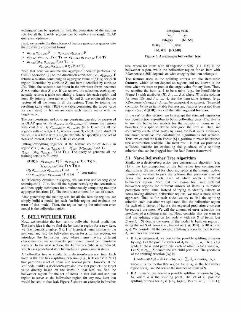
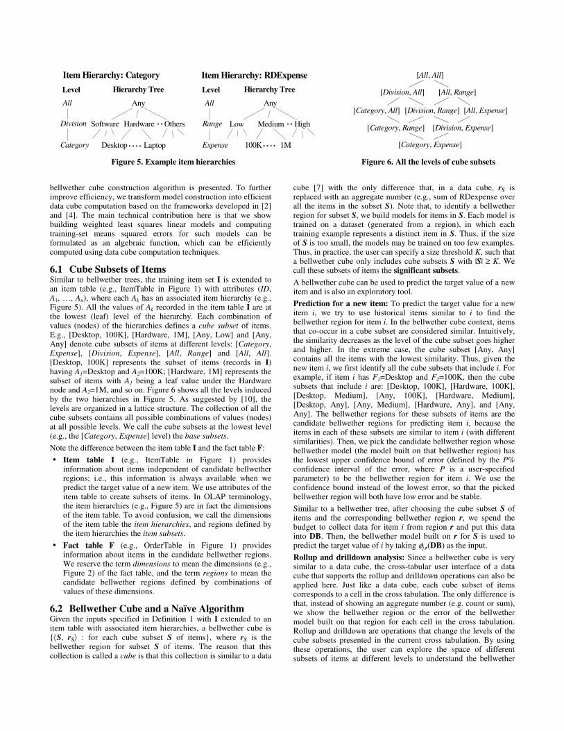
6. BELLWETHER CUBE Similar to a bellwether tree, a bellwether cube finds different bellwether regions for different subsets of items. However, unlike a bellwether tree, in which item subsets are induced by the tree structure, the item subsets in a bellwether cube are defined by item hierarchies. Figure 5 shows an example of two item hierarchies. For example, [Hardware, Low] represents the subset of items that belong to the Hardware division and have low R&D expenses, and the bellwether region for it may be different from the bellwether region for item subset [Desktop, Any]. A bellwether cube systematically finds the bellwether region for each such cube subset of items induced by the item hierarchies. It not only can be used to predict the target value of a new item, but also is an exploratory tool for rollup and drilldown analysis.

In the rest of this section, we first define bellwether cubes and show how to use them to perform bellwether-based prediction and conduct rollup and drilldown analysis. Then, a single-scan

Naïve Bellwether Tree Algorithm

call SplitNode(Root node u, Item set I); Prune the resulting tree; function SplitNode(Node v, Item set S)

if the termination condition holds then return; foreach possible splitting criterion c

foreach child partition Sp created by c

Find the bellwether region for Sp;

Evaluate Goodness(c); Pick criterion c* that has the maximum goodness value; Create child nodes v1, …, vn based on c*;

foreach child node vp

call SplitNode(vp, Sp);

RF Bellwether Tree Algorithm

foreach level l of the tree foreach (active node v at level l, splitting criterion c)

foreach (child partition p) Set MinError[v, c, p] = ∞; (In the following, scan the entire training data once) foreach feasible region r ∈ R

Read in training set Dr for region r; foreach active node v at level l

foreach possible splitting criterion c foreach child partition Sp created by c

Build a model hr on region r for Sp;

if Error(hr | Sp) < MinError[v, c, p] then

MinError[v, c, p] = Error(hr | Sp);

Size[v, c, p] = |Sp|;

foreach active node v at level l foreach possible splitting criterion c

Compute Goodness(c) from MinError[v, c, p] and Size[v, c, p], for all p;

Split v based on c* that has the best goodness value;

Figure 4. Bellwether tree algorithms

bellwether cube construction algorithm is presented. To further improve efficiency, we transform model construction into efficient data cube computation based on the frameworks developed in [2] and [4]. The main technical contribution here is that we show building weighted least squares linear models and computing training-set means squared errors for such models can be formulated as an algebraic function, which can be efficiently computed using data cube computation techniques.

6.1 Cube Subsets of Items Similar to bellwether trees, the training item set I is extended to an item table (e.g., ItemTable in Figure 1) with attributes (ID, A1, …, An), where each Ak has an associated item hierarchy (e.g., Figure 5). All the values of Ak recorded in the item table I are at the lowest (leaf) level of the hierarchy. Each combination of values (nodes) of the hierarchies defines a cube subset of items. E.g., [Desktop, 100K], [Hardware, 1M], [Any, Low] and [Any, Any] denote cube subsets of items at different levels: [Category, Expense], [Division, Expense], [All, Range] and [All, All]. [Desktop, 100K] represents the subset of items (records in I) having A1=Desktop and A2=100K; [Hardware, 1M] represents the subset of items with A1 being a leaf value under the Hardware node and A2=1M, and so on. Figure 6 shows all the levels induced by the two hierarchies in Figure 5. As suggested by [10], the levels are organized in a lattice structure. The collection of all the cube subsets contains all possible combinations of values (nodes) at all possible levels. We call the cube subsets at the lowest level (e.g., the [Category, Expense] level) the base subsets.

Note the difference between the item table I and the fact table F:

� Item table I (e.g., ItemTable in Figure 1) provides information about items independent of candidate bellwether regions; i.e., this information is always available when we predict the target value of a new item. We use attributes of the item table to create subsets of items. In OLAP terminology, the item hierarchies (e.g., Figure 5) are in fact the dimensions of the item table. To avoid confusion, we call the dimensions of the item table the item hierarchies, and regions defined by the item hierarchies the item subsets.

� Fact table F (e.g., OrderTable in Figure 1) provides information about items in the candidate bellwether regions. We reserve the term dimensions to mean the dimensions (e.g., Figure 2) of the fact table, and the term regions to mean the candidate bellwether regions defined by combinations of values of these dimensions.

6.2 Bellwether Cube and a Naïve Algorithm Given the inputs specified in Definition 1 with I extended to an item table with associated item hierarchies, a bellwether cube is {⟨S, rS⟩ : for each cube subset S of items}, where rS is the bellwether region for subset S of items. The reason that this collection is called a cube is that this collection is similar to a data

cube [7] with the only difference that, in a data cube, rS is replaced with an aggregate number (e.g., sum of RDexpense over all the items in the subset S). Note that, to identify a bellwether region for subset S, we build models for items in S. Each model is trained on a dataset (generated from a region), in which each training example represents a distinct item in S. Thus, if the size of S is too small, the models may be trained on too few examples. Thus, in practice, the user can specify a size threshold K, such that a bellwether cube only includes cube subsets S with |S| ≥ K. We call these subsets of items the significant subsets.

A bellwether cube can be used to predict the target value of a new item and is also an exploratory tool.

Prediction for a new item: To predict the target value for a new item i, we try to use historical items similar to i to find the bellwether region for item i. In the bellwether cube context, items that co-occur in a cube subset are considered similar. Intuitively, the similarity decreases as the level of the cube subset goes higher and higher. In the extreme case, the cube subset [Any, Any] contains all the items with the lowest similarity. Thus, given the new item i, we first identify all the cube subsets that include i. For example, if item i has F1=Desktop and F2=100K, then the cube subsets that include i are: [Desktop, 100K], [Hardware, 100K], [Desktop, Medium], [Any, 100K], [Hardware, Medium], [Desktop, Any], [Any, Medium], [Hardware, Any], and [Any, Any]. The bellwether regions for these subsets of items are the candidate bellwether regions for predicting item i, because the items in each of these subsets are similar to item i (with different similarities). Then, we pick the candidate bellwether region whose bellwether model (the model built on that bellwether region) has the lowest upper confidence bound of error (defined by the P% confidence interval of the error, where P is a user-specified parameter) to be the bellwether region for item i. We use the confidence bound instead of the lowest error, so that the picked bellwether region will both have low error and be stable.

Similar to a bellwether tree, after choosing the cube subset S of items and the corresponding bellwether region r, we spend the budget to collect data for item i from region r and put this data into DB. Then, the bellwether model built on r for S is used to predict the target value of i by taking φj,r(DB) as the input.

Rollup and drilldown analysis: Since a bellwether cube is very similar to a data cube, the cross-tabular user interface of a data cube that supports the rollup and drilldown operations can also be applied here. Just like a data cube, each cube subset of items corresponds to a cell in the cross tabulation. The only difference is that, instead of showing an aggregate number (e.g. count or sum), we show the bellwether region or the error of the bellwether model built on that region for each cell in the cross tabulation. Rollup and drilldown are operations that change the levels of the cube subsets presented in the current cross tabulation. By using these operations, the user can explore the space of different subsets of items at different levels to understand the bellwether

AnyAll

Division

Category

Item Hierarchy: Category

HardwareSoftware

Desktop Laptop

Others

AnyAll

Range

Expense

Item Hierarchy: RDExpense

MediumLow High

100K 1M [Category, Expense]

[Category, Range] [Division, Expense]

[Category, All] [Division, Range] [All, Expense]

[Division, All] [All, Range]

[All, All]

Level Hierarchy Tree Level Hierarchy Tree

Figure 5. Example item hierarchies Figure 6. All the levels of cube subsets

behavior of the database. We omit the details of the user interface, and note that a more thorough treatment of applying the data cube interface to predictive models can be found in [2].

Naïve algorithm: If we have unlimited resources, we can just enumerate the cube subsets of items, and for each cube subset, apply the basic bellwether search algorithm to find the bellwether region for that subset.

6.3 Single-Scan Bellwether Cube Algorithm It is obvious that the naïve algorithm is very inefficient, since for each cube subset of items, we need to solve a basic bellwether problem for that subset. However, because the cube subsets are nested, by carefully sharing the computation, it is possible to improve the efficiency. Also, if we have large enough memory, we can build a bellwether cube in a single scan over the entire training data, which consists of the training sets for all the feasible regions. In this subsection, we describe the single-scan technique. We discuss the technique that exploits shared computation in the next subsection.

In the following, we assume the size of main memory is at least O(n), where n is the number of significant cube subsets of items; i.e., the main memory is large enough to simultaneously hold a small amount of size-fixed data for each significant cube subset. Since the number of items is usually modest, the number of significant cube subsets of items is usually also modest. Thus, it is reasonable to assume the number of significant cube subsets can fit in memory. If the number of significant cube subsets cannot fit in memory, we can partition these cube subsets into several parts such that each part fits in memory. However, for simplicity, we omit the details.

Let rS denote the bellwether region for item subset S. By definition, Error(hrS

| S) = minr∈R Error(hr | S). Thus, similar to the RF bellwether tree algorithm, we can keep an entry for each cube subset S of items in memory, and scan the entire training data (i.e., going through each r ∈ R) once to find the region rS that has the minimum error. The algorithm is shown in Figure 7. Note that we omit the details about how to select significant cube subsets of items because this can be done by an iceberg query, for which computation techniques are well known [1, 19].

Lemma 2. The single-scan bellwether cube algorithm outputs the same bellwether cube as the naïve algorithm in a single scan over the entire training data.

6.4 Optimizing Repeated Model Construction Now, we describe the techniques to share the computation of building models on nested subsets of items. Note that, in the single-scan bellwether cube algorithm, we build a model for each significant cube subset of items, and these cube subsets may be nested. For example, we may build models for cube subsets: [Hardware, Medium], [Any, Medium], [Hardware, Any], and [Any, Any], where the first one is included in the following two, and the first three are included in the last one.

Let us first review how to take advantage of this nested-subset structure in regular data cube computation, where we want to compute an aggregate function (e.g., sum and average) for each cube subset. It is well known that if the aggregate function is distributive or algebraic, the aggregate values for all the cube subsets can be computed efficiently [7]. Let S1, …, Sn be subsets of items that partition S; i.e., ∪i Si = S, Si ∩ Sj = ∅, for i ≠ j. An aggregate function f is distributive if there is a function q such that f(S) = q({f(Si) : i = 1, …, n}). SUM, and COUNT are examples of distributive functions. An aggregate function f is algebraic if there are a function g that returns a fixed-length tuple and a function q

such that f(S) = q({g(Si) : i = 1, …, n}). All distributive functions are algebraic, and AVG is another example of a distributive function, where g(Si) returns ⟨SUM(Si), COUNT(Si)⟩, and q sums up all the sums and counts separately and then divides the total sum by the total count. See [7] for details.

Observation 1. Fixing region r, if Error(hr | S) is a distributive or algebraic function of S, then data cube computation techniques can be directly applied to efficiently compute the errors for all the (significant) cube subsets of items for region r.

Note that knowing Error(hr | S) for all feasible region r and all significant cube subset S of items is sufficient to build a bellwether cube. Thus, we focus on error computation, instead of model construction, although model construction is embedded in the error computation.

Following the observation, if Error(hr | S) can be computed by distributive or algebraic aggregate functions, we can replace “foreach significant cube subset S of items, build a model hr on r for S” (i.e., line 7-8 of Figure 7) with a data cube query that returns the error value for each significant cube subset. We omit the details of the data cube computation, for it is well known.

Now the question is how to make Error(hr | S) a distributive or algebraic aggregate function of S. It depends on what kind of predictive model is used. For classification models, Chen et al. [2] developed a scoring function decomposition technique, which allows test-set-based accuracy (equivalently, error) computation to be treated as computing distributive or algebraic aggregate functions if the model used is distributively or algebraically decomposable. For indecomposable models, an approximation technique called probability-based ensemble was also proposed to make the model distributively decomposable with a small accuracy drop. These techniques can be directly applied here.

For regression models, Chen et al. [4] developed a technique to efficiently build ordinary least squares (OLS) linear regression models for nested cube subsets. In the following, we extend their technique in two ways. First, our technique not only can handle OLS linear regression models, but also weighted least squares (WLS) linear regression models, which are usually used in Statistics to handle aggregated target values (e.g., total sales). Second, our technique directly transforms the computation of training-set mean squared errors of WLS linear models to the computation of algebraic aggregate functions. Note that because linear models are simple models, training-set errors are usually good estimates of the true errors of the models. Our experimental results also suggest that the behavior of training-set errors is very similar to that of cross-validation errors for linear models.

We first review some basics of linear regression models (see [18] for details). Let X = (Xi,j) be an n×p matrix, where each row is a

Select all the significant cube subsets of items by an iceberg cube query over I;

foreach significant cube subset S of items Set MinError[S] = ∞;

(In the following, scan the entire training data once) foreach feasible region r ∈ R

foreach significant cube subset S of items Build a model hr on r for S; if Error(hr | S) < MinError[S] then

MinError[S] = ∞; BellwetherRegion[S] = r;

Output BellwetherRegion[S] for each S;

Figure 7. Single-scan bellwether cube algorithm

training example, and each column represents a feature; i.e., Xi,j is the jth feature value1 of example i. Note that we have n training examples, each of which has p feature values. For simplicity, all the features are assumed to be numeric. Let Y = (Yi) be a column vector with length n, where Yi is the target value of the ith example (i.e., row) in X. Let W = (Wi,j) be an n×n positive diagonal matrix (i.e., Wi,j = 0 for i ≠ j and Wi,i > 0 for i = 1, …, n) which specifies the weight for each example; i.e., Wi,i is the weight for the ith example in X. A linear regression model is written as Yi = ∑j Xi,j βj + εi, where βj, j = 1, …, p, are the model parameters, and εi is the error term for the ith example. We use a p-element column vector ββββ to denote all the model parameters. The OLS linear model is the ββββ that minimizes ∑i (Yi −∑j Xi,j βj)

2 and the WLS linear model is the ββββ that minimizes ∑i Wi,i(Yi −∑j Xi,j βj)

2. Note that, when Wi,i = 1 for all i, the WLS linear model reduces to the OLS linear model. Thus, we only consider the WLS linear model. According to [18], the WLS linear model is:

ββββWLS = (X′WX)−1(X′WY),

where X′ denotes the matrix transpose of X. By a straightforward matrix derivation, we obtain the weighted sum of squared errors:

∑i Wi,i(Yi −∑j Xi,j βj)2 = (Y − XββββWLS)′W(Y − XββββWLS)

= Y′WY − (X′WY)′(X′WX)−1(X′WY),

and the weighted mean squared error is the above quantity divided by n−p, which is the number of degrees of freedom. Note that Y′WY is a number, X′WX is a p×p matrix, and X′WY is a p×1 vector. None of their sizes depend on the number of examples (i.e., n), but having these is sufficient to obtain the WLS linear model and its training-set (weighted) mean squared error.

Let S be a cube subset of items, and S1, …, Sm be subsets of S that partition S. We use X, Y, W and Xk, Yk, Wk to denote the feature matrix, target-value vector and weight matrix for S and Sk (k = 1, …, m), respectively. Let SSEr(S) denote the (weighted) sum of squared errors of the model hr trained on a given region r using items in S. Then, we have the following theorem.

Theorem 1. SSEr(S) is an algebraic aggregate function of S; i.e., SSEr(S) = q({g(Si) : i = 1, …, n}), where

g(Sk) = ⟨Yk′WkYk, Xk′WkXk, Xk′WkYk⟩, and q({g(Sk)}) = (∑k Yk′WkYk)−(∑k Xk′WkYk)′(∑k Xk′WkXk)

−1(∑k Xk′WkYk).

Proof: (1) The size of the returned value of g(Sk) is 1 + p×p + p, which is fixed (i.e., independent of the sizes of S and Sk). (2) By a straightforward matrix derivation, we can see that Y′WY = ∑k Yk′WkYk, X′WX = ∑k Xk′WkXk and X′WY = ∑k Xk′WkYk. Thus, q({g(Si)}) indeed returns the SSEr(S). �

7. EXPERIMENTAL RESULTS In this section, we present the experimental results. We first show that bellwether regions do exist in real datasets, and bellwether trees and cubes may improve the prediction accuracy over the bellwether region found by the basic bellwether search. We then demonstrate efficiency and scalability of the proposed algorithms.

7.1 Mail Order Dataset The mail order dataset contains transaction records of a real catalog company for the year 1996. It contains 1,515 items and 4,591,581 transactions. After removing outliers, 1,012 items and the associated 4,030,335 transactions were selected for the following analysis. The fact table contains transactions of the orders, each of which records an order of a single item at a specific time and from a specific location with the net profit

1 To include a constant term in the regression model, set Xi,1 always to 1.

earned from that order. A candidate region is defined by a time interval (e.g., first two months) and a location (e.g., Midwest) in the US. The time and location dimensions are similar to those in Figure 2 with the following differences. For the time dimension, instead of weeks, we consider the 1st month, 1-2 months, …, and 1-10 months. For the location dimension, the levels are State, Division, Region, and All. The cost of each region is defined by m⋅n, where m is the number of months in the time interval and n is the number of zip code areas in the location divided by 100. The goal is to find a cost-effective region such that the features generated from that region can best predict the total profit of an item in the US over the entire time interval (10 months). The features of an item are the profit and the number of orders in a region, and also information from the mailed catalogs. We use the OLS linear regression model as the predictive model, and use 10-fold cross-validation root mean squared error as the error measure.

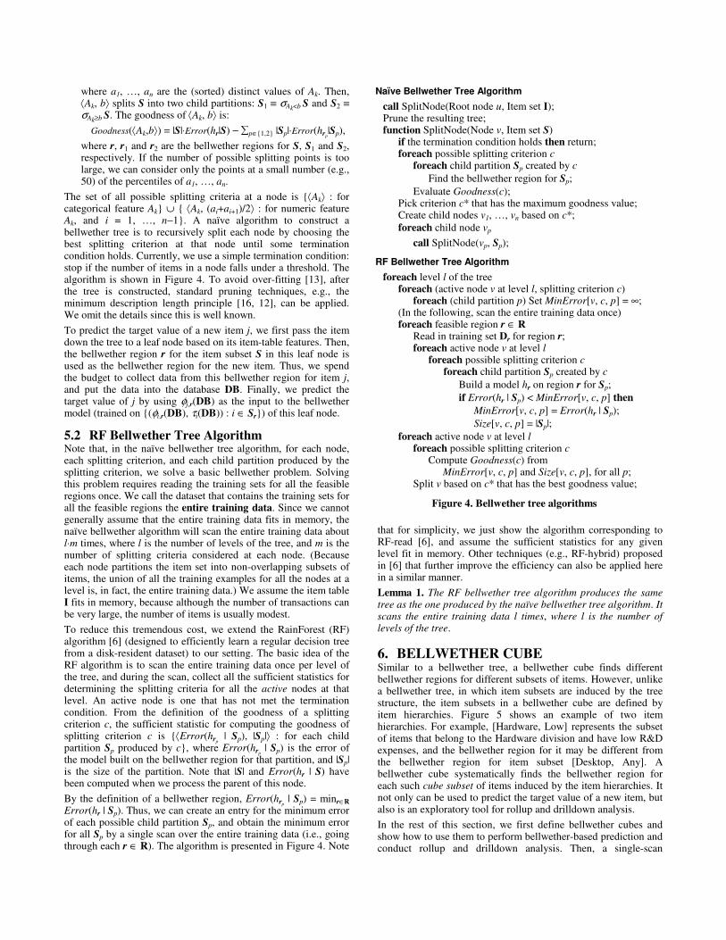
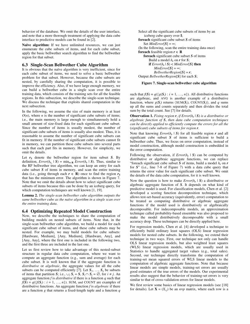
Figure 7 (a) shows the error of the bellwether model as a function of the budget. To understand how well a bellwether model performs, we plot the following curves.

� Bel Err: This curve shows the error of the bellwether model (i.e., the model built using data from the bellwether region). Each point represents the error of the bellwether model with a cost under a specific budget.

� Avg Err: This curve shows the average error, on which each point represents the average error of all the regions with costs under a specific budget.

� Smp Err: This curve shows the performance of a random sampling approach, in which we randomly select a collection of regions such that the cost of the collection is at most the specified budget. Note that this collection may not correspond to any OLAP-style region (defined in Section 3.1), which we consider as the candidates in the bellwether search.

The result in Figure 7 (a) shows that at budget around 50, the error of the bellwether model converges, which means we cannot increase the performance of the model by increasing the budget. The bellwether region found is [1-8, MD], i.e., the first eight months in the state of Maryland. Also, the bellwether model performs better than the random sampling approach and significantly better than the average case.

Figure 7 (b) shows the uniqueness of bellwether regions. Each point on the curve labelled with P% represents the fraction of regions that have a model with error within P% confidence interval of the error of the bellwether model under a specific budget. A high fraction means the bellwether region found is indistinguishable from other regions under the budget. A low fraction means the bellwether is almost unique, because almost no other region can perform as well as the bellwether one. As shown in the figure, from budget 35 to 85, the bellwether regions found are almost unique.

Figure 7 (c) shows the plot of error vs. budget using the training-set error, instead of the cross-validation error. Note that it is almost exactly the same as Figure 7 (a). This verifies that for simple models such as linear models, training-set error usually approximates cross-validation error, but can be computed much more efficiently.

Finally, we evaluate item-centric bellwether-based prediction on the mail order dataset. The result is shown in Figure 8. We consider three methods. The bellwether tree (labelled Tree), the bellwether cube (labelled Cube) and the method that simply uses the bellwether region found by the basic bellwether search (labelled Basic). The 10-fold cross-validation prediction errors for each method at various budgets are reported in Figure 8. The

result shows that from budget 10 to 30, both the bellwether cube and the bellwether tree improve accuracy over basic bellwether search. However, the improvement is not significant. The reason might be that there is not too much difference between different subsets of items in this particular dataset.

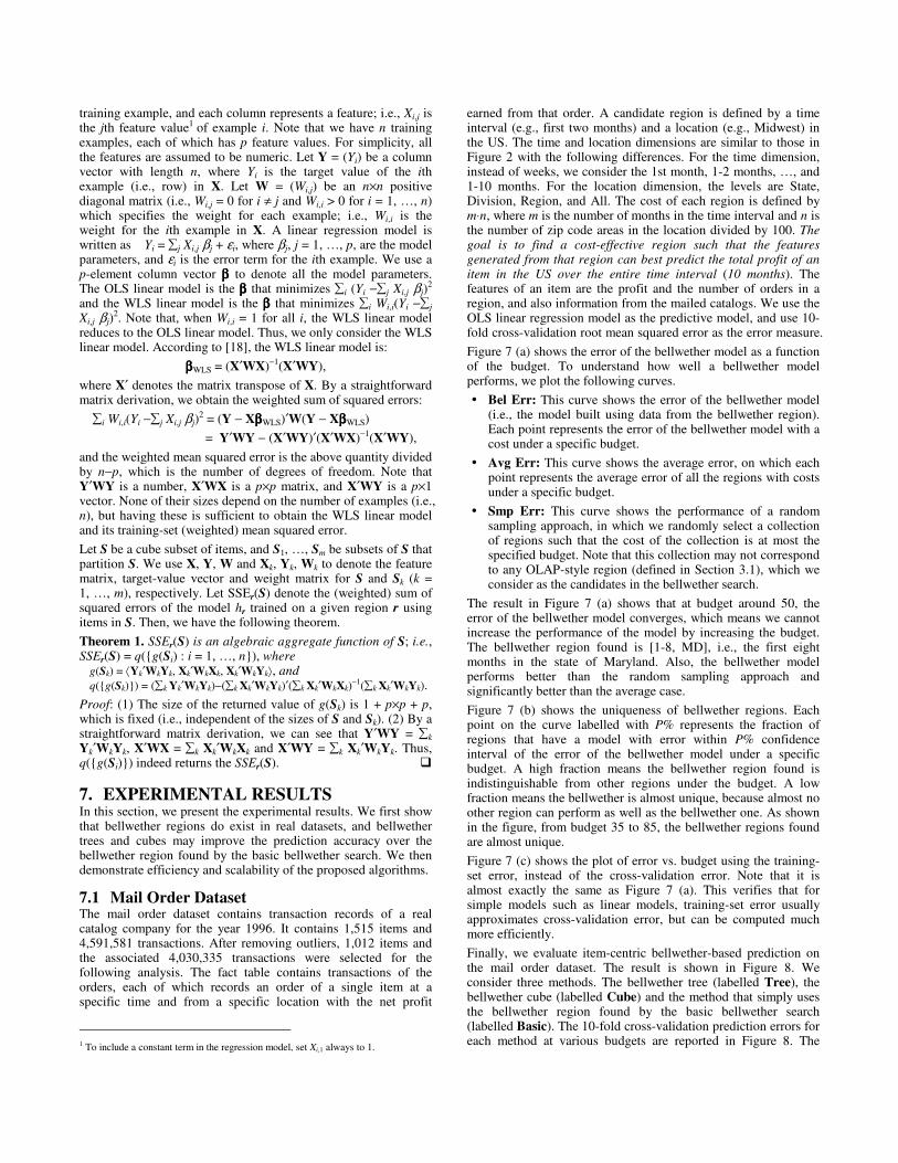
7.2 Book Store Dataset Next, we show the results on another real dataset where there is no clear bellwether region. The book store dataset is a sample from a large bookstore company with stores spread across the United States. The dataset obtained contains transactional data of books sold for the year 2004 in five states of USA totaling 900,000 transactions and about 43,000 books; of which we used around a thousand most occurring books, since many books only have very few transaction records. There are 116 stores spread across 86 cities in the five given states. Similar to the mail order dataset, we consider time and location to be dimension attributes that define candidate regions. Similarly, OLS linear regression models and cross-validation errors are used to determine bellwether regions.

The result is shown in Figure 9. Although in Figure 9 (a) the error of the bellwether model seems to converge at budget 200, we cannot identify a bellwether region with high confidence, since as shown in Figure 9 (b), there is still a relatively large fraction of other regions that are indistinguishable from the one returned by the basic search algorithm. The reason that we cannot find clear bellwether regions might be that (1) there is actually no unique bellwether region at each budget point, or (2) the dataset is too small. Note that this dataset does not contain all the transaction records for the stores we have. Rather, it is a relatively small sample of the actual data warehouse. The prediction errors of the basic, tree and cube methods are shown in Figure 9 (c). There is no clear winner to be found.

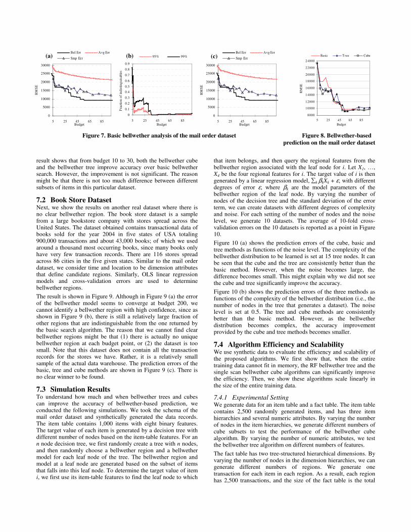
7.3 Simulation Results To understand how much and when bellwether trees and cubes can improve the accuracy of bellwether-based prediction, we conducted the following simulations. We took the schema of the mail order dataset and synthetically generated the data records. The item table contains 1,000 items with eight binary features. The target value of each item is generated by a decision tree with different number of nodes based on the item-table features. For an n node decision tree, we first randomly create a tree with n nodes, and then randomly choose a bellwether region and a bellwether model for each leaf node of the tree. The bellwether region and model at a leaf node are generated based on the subset of items that falls into this leaf node. To determine the target value of item i, we first use its item-table features to find the leaf node to which

that item belongs, and then query the regional features from the bellwether region associated with the leaf node for i. Let X1, …, X4 be the four regional features for i. The target value of i is then generated by a linear regression model, ∑k βkXk + ε, with different degrees of error ε, where βk are the model parameters of the bellwether region of the leaf node. By varying the number of nodes of the decision tree and the standard deviation of the error term, we can create datasets with different degrees of complexity and noise. For each setting of the number of nodes and the noise level, we generate 10 datasets. The average of 10-fold cross-validation errors on the 10 datasets is reported as a point in Figure 10.

Figure 10 (a) shows the prediction errors of the cube, basic and tree methods as functions of the noise level. The complexity of the bellwether distribution to be learned is set at 15 tree nodes. It can be seen that the cube and the tree are consistently better than the basic method. However, when the noise becomes large, the difference becomes small. This might explain why we did not see the cube and tree significantly improve the accuracy.

Figure 10 (b) shows the prediction errors of the three methods as functions of the complexity of the bellwether distribution (i.e., the number of nodes in the tree that generates a dataset). The noise level is set at 0.5. The tree and cube methods are consistently better than the basic method. However, as the bellwether distribution becomes complex, the accuracy improvement provided by the cube and tree methods becomes smaller.

7.4 Algorithm Efficiency and Scalability We use synthetic data to evaluate the efficiency and scalability of the proposed algorithms. We first show that, when the entire training data cannot fit in memory, the RF bellwether tree and the single scan bellwether cube algorithms can significantly improve the efficiency. Then, we show these algorithms scale linearly in the size of the entire training data.

7.4.1 Experimental Setting We generate data for an item table and a fact table. The item table contains 2,500 randomly generated items, and has three item hierarchies and several numeric attributes. By varying the number of nodes in the item hierarchies, we generate different numbers of cube subsets to test the performance of the bellwether cube algorithm. By varying the number of numeric attributes, we test the bellwether tree algorithm on different numbers of features.

The fact table has two tree-structured hierarchical dimensions. By varying the number of nodes in the dimension hierarchies, we can generate different numbers of regions. We generate one transaction for each item in each region. As a result, each region has 2,500 transactions, and the size of the fact table is the total

0

5000

10000

15000

20000

25000

30000

5 25 45 65 85Budget

RM

SE

Bel Err Avg Err

Smp Err

0

0.1

0.2

0.3

0.4

0.5

0.6

0.7

0.8

0.9

5 25 45 65 85Budget

Fra

ctio

n o

f in

dis

tin

gu

isab

les

95% 99%

0

5000

10000

15000

20000

25000

30000

5 25 45 65 85Budget

RM

SE

Bel Err Avg Err

Smp Err

8000

10000

12000

14000

16000

18000

20000

22000

24000

5 25 45 65 85

Budget

RM

SE

Basic T ree Cube

Figure 7. Basic bellwether analysis of the mail order dataset Figure 8. Bellwether-based

prediction on the mail order dataset

(a) (b) (c)

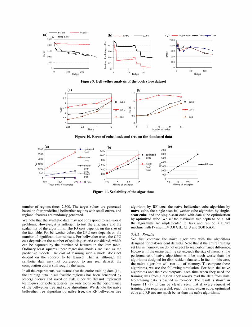
number of regions times 2,500. The target values are generated based on four predefined bellwether regions with small errors, and regional features are randomly generated.

We note that the synthetic data may not correspond to real-world problems. However, it is sufficient to test the efficiency and the scalability of the algorithms. The IO cost depends on the size of the fact table. For bellwether cubes, the CPU cost depends on the number of significant item subsets. For bellwether trees, the CPU cost depends on the number of splitting criteria considered, which can be captured by the number of features in the item table. Ordinary least squares linear regression models are used as the predictive models. The cost of learning such a model does not depend on the concept to be learned. That is, although the synthetic data may not correspond to any real dataset, the computation cost is still roughly the same.

In all the experiments, we assume that the entire training data (i.e., the training data in all feasible regions) has been generated by iceberg queries and saved on disk. Since we did not implement techniques for iceberg queries, we only focus on the performance of the bellwether tree and cube algorithms. We denote the naïve bellwether tree algorithm by naïve tree, the RF bellwether tree

algorithm by RF tree, the naïve bellwether cube algorithm by naïve cube, the single-scan bellwether cube algorithm by single-scan cube, and the single-scan cube with data cube optimization by optimized cube. We set the maximum tree depth to be 7. All the algorithms are implemented in Java and run on a Linux machine with Pentium IV 3.0 GHz CPU and 2GB RAM.

7.4.2 Results We first compare the naïve algorithms with the algorithms designed for disk-resident datasets. Note that if the entire training set fits in memory, we do not expect to see performance difference. However, if the entire training set exceeds the size of memory, the performance of naïve algorithms will be much worse than the algorithms designed for disk-resident datasets. In fact, in this case, the naïve algorithm will run out of memory. To compare these algorithms, we use the following simulation. For both the naïve algorithms and their counterparts, each time when they need the training data from a region, they always read the data from disk. No training data is cached in memory. The result is shown in Figure 11 (a). It can be clearly seen that if every request of training data requires a disk read, the single-scan cube, optimized cube and RF tree are much better than the naïve algorithms.

0

500

1000

1500

2000

2500

0 100 200Budget

RM

SE

Bel Err Avg Err

Samp Error

0

0.2

0.4

0.6

0.8

1

0 100 200Budget

Fra

cti

on

of

ind

isti

ng

uis

ab

les

0 .95% 0.99%

0

500

1000

1500

2000

2500

0 100 200

Budget

RM

SE

SingleRegion Cube T ree

Figure 9. Bellwether analysis of the book store dataset

0

0.5

1

1.5

2

2.5

3

0.05 0.5 1 2Noise

RM

SE

cube

basic

tree

0

0.5

1

1.5

2

3 7 15 31 63Number of nodes

RM

SE

cube

basic

tree

Figure 10. Error of cube, basic and tree on the simulated data

0

500

1000

1500

2000

2500

3000

100 200 300

Thousands of examples

Se

c

optimized

cube

naive

cube

single-

scan

cubenaive

tree

RF tree

0

200

400

600

800

1000

1200

2.5 5 7.5 10Millions of examples

Se

c

optimized

cube

single-

scan

cube

0

1000

2000

3000

4000

5000

6000

7000

2.5 5 7.5 10Millions of examples

Se

c

RF tree

Figure 11. Scalability of the algorithms

(a) (b) (c)

(a) (b)

(a) (b) (c)

Next, we show the scalability of the single-scan cube, the optimized cube (in Figure 11 (b)) and the RF tree (in Figure 11 (c)). These algorithms all scale linearly in the number of examples in the entire training data. Also the optimized cube has better performance than the single-scan cube. Note that the RF tree takes more time than the cubes. This is because RF tree scans the entire training data once per level of the tree, while the cubes only scan the entire training data once. Techniques developed in [6] can further reduce the cost of the RF tree. Also, the cubes only use the three item hierarchies, but the RF tree uses 4 additional numeric item features.

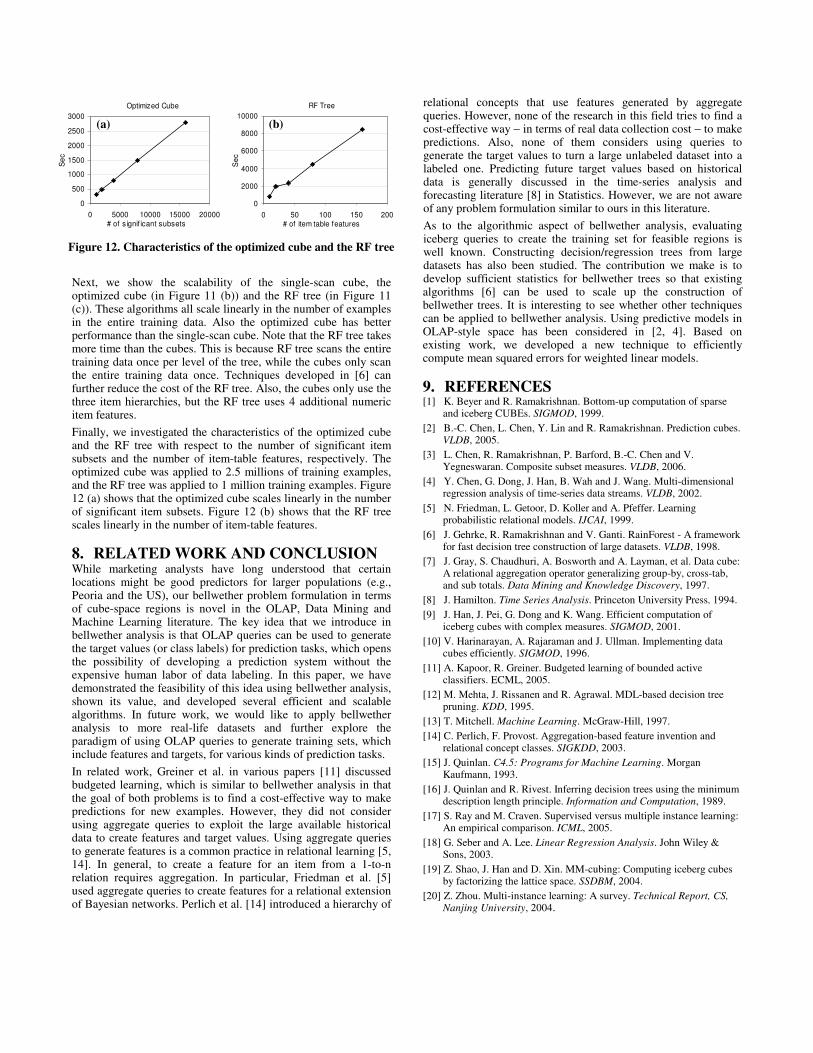
Finally, we investigated the characteristics of the optimized cube and the RF tree with respect to the number of significant item subsets and the number of item-table features, respectively. The optimized cube was applied to 2.5 millions of training examples, and the RF tree was applied to 1 million training examples. Figure 12 (a) shows that the optimized cube scales linearly in the number of significant item subsets. Figure 12 (b) shows that the RF tree scales linearly in the number of item-table features.

8. RELATED WORK AND CONCLUSION While marketing analysts have long understood that certain locations might be good predictors for larger populations (e.g., Peoria and the US), our bellwether problem formulation in terms of cube-space regions is novel in the OLAP, Data Mining and Machine Learning literature. The key idea that we introduce in bellwether analysis is that OLAP queries can be used to generate the target values (or class labels) for prediction tasks, which opens the possibility of developing a prediction system without the expensive human labor of data labeling. In this paper, we have demonstrated the feasibility of this idea using bellwether analysis, shown its value, and developed several efficient and scalable algorithms. In future work, we would like to apply bellwether analysis to more real-life datasets and further explore the paradigm of using OLAP queries to generate training sets, which include features and targets, for various kinds of prediction tasks.

In related work, Greiner et al. in various papers [11] discussed budgeted learning, which is similar to bellwether analysis in that the goal of both problems is to find a cost-effective way to make predictions for new examples. However, they did not consider using aggregate queries to exploit the large available historical data to create features and target values. Using aggregate queries to generate features is a common practice in relational learning [5, 14]. In general, to create a feature for an item from a 1-to-n relation requires aggregation. In particular, Friedman et al. [5] used aggregate queries to create features for a relational extension of Bayesian networks. Perlich et al. [14] introduced a hierarchy of

relational concepts that use features generated by aggregate queries. However, none of the research in this field tries to find a cost-effective way − in terms of real data collection cost − to make predictions. Also, none of them considers using queries to generate the target values to turn a large unlabeled dataset into a labeled one. Predicting future target values based on historical data is generally discussed in the time-series analysis and forecasting literature [8] in Statistics. However, we are not aware of any problem formulation similar to ours in this literature.

As to the algorithmic aspect of bellwether analysis, evaluating iceberg queries to create the training set for feasible regions is well known. Constructing decision/regression trees from large datasets has also been studied. The contribution we make is to develop sufficient statistics for bellwether trees so that existing algorithms [6] can be used to scale up the construction of bellwether trees. It is interesting to see whether other techniques can be applied to bellwether analysis. Using predictive models in OLAP-style space has been considered in [2, 4]. Based on existing work, we developed a new technique to efficiently compute mean squared errors for weighted linear models.

9. REFERENCES [1] K. Beyer and R. Ramakrishnan. Bottom-up computation of sparse

and iceberg CUBEs. SIGMOD, 1999.

[2] B.-C. Chen, L. Chen, Y. Lin and R. Ramakrishnan. Prediction cubes. VLDB, 2005.

[3] L. Chen, R. Ramakrishnan, P. Barford, B.-C. Chen and V. Yegneswaran. Composite subset measures. VLDB, 2006.

[4] Y. Chen, G. Dong, J. Han, B. Wah and J. Wang. Multi-dimensional regression analysis of time-series data streams. VLDB, 2002.

[5] N. Friedman, L. Getoor, D. Koller and A. Pfeffer. Learning probabilistic relational models. IJCAI, 1999.

[6] J. Gehrke, R. Ramakrishnan and V. Ganti. RainForest - A framework for fast decision tree construction of large datasets. VLDB, 1998.

[7] J. Gray, S. Chaudhuri, A. Bosworth and A. Layman, et al. Data cube: A relational aggregation operator generalizing group-by, cross-tab, and sub totals. Data Mining and Knowledge Discovery, 1997.

[8] J. Hamilton. Time Series Analysis. Princeton University Press, 1994.

[9] J. Han, J. Pei, G. Dong and K. Wang. Efficient computation of iceberg cubes with complex measures. SIGMOD, 2001.

[10] V. Harinarayan, A. Rajaraman and J. Ullman. Implementing data cubes efficiently. SIGMOD, 1996.

[11] A. Kapoor, R. Greiner. Budgeted learning of bounded active classifiers. ECML, 2005.

[12] M. Mehta, J. Rissanen and R. Agrawal. MDL-based decision tree pruning. KDD, 1995.

[13] T. Mitchell. Machine Learning. McGraw-Hill, 1997.

[14] C. Perlich, F. Provost. Aggregation-based feature invention and relational concept classes. SIGKDD, 2003.

[15] J. Quinlan. C4.5: Programs for Machine Learning. Morgan Kaufmann, 1993.

[16] J. Quinlan and R. Rivest. Inferring decision trees using the minimum description length principle. Information and Computation, 1989.

[17] S. Ray and M. Craven. Supervised versus multiple instance learning: An empirical comparison. ICML, 2005.

[18] G. Seber and A. Lee. Linear Regression Analysis. John Wiley & Sons, 2003.

[19] Z. Shao, J. Han and D. Xin. MM-cubing: Computing iceberg cubes by factorizing the lattice space. SSDBM, 2004.

[20] Z. Zhou. Multi-instance learning: A survey. Technical Report, CS,

Nanjing University, 2004.

Optimized Cube

0

500

1000

1500

2000

2500

3000

0 5000 10000 15000 20000# of s ignif icant subsets

Se

c

RF Tree

0

2000

4000

6000

8000

10000

0 50 100 150 200# of item table features

Se

c

Figure 12. Characteristics of the optimized cube and the RF tree

(a) (b)