Embed Size (px)
Citation preview
THE ROLE OF ELEVATION ON TEMPERATURE TRENDS IN THE WESTERN UNITED STATES:
A COMPARISON OF TWO STATISTICAL METHODS
By
Ruben J Behnke
A thesis submitted in partial fulfillment of the requirements for the degree of
Master of Science
(Atmospheric and Oceanic Science)
UNIVERSITY OF WISCONSIN – MADISON
2011

ii
Acknowledgements
I would like to express my sincere gratitude to my research and academic advisor,
Ankur Desai. He has provided me with the advice, encouragement, and help I needed to
successfully complete my degree and my research. I would also like to thank Dan Vimont
and Chris Kucharik for taking the time to provide comments and edit my thesis, and
especially Steve Vavrus for providing me with the opportunity for me to stay at UW
Madison and finish my degree. Also, a sincere thank you goes to my fellow lab members
and AOS graduate students for their encouragement and comments.
I would also like to thank Sam Batzli for taking the time to teach me a great deal of
GIS and also Bjorn Brooks for taking the time to help me with the computational aspects of
the clustering process. I could not have produced all the maps and data without their help.
Finally, I am grateful to both the office staff of The PRISM Group at OSU and Clark Labs,
Clark University for providing me with a great deal of assistance with data and tool usage.
This research was funded by grants from the Centers for Disease Control and the
Department of Energy.
iii
Contents
1. Introduction 1
2. Background 3
2.1 Topoclimate/microclimate 3
2.2 Literature Review 5
2.2.1 Previous Studies 5
2.2.2 Global and North American Temperature Trends 7
2.3 Free Air vs. Surface Meteorology 10
3. Objectives 13
3.1 Hypotheses 13
3.2 Study Regions 14
4. Methodology 15
4.1 Data Set – PRISM 16
4.2 Previous Research 18
4.3 Definition of Mountainous Regions 22
4.4 Statistical Methods 27
4.4.1 Least Squares Linear Regression 27
4.4.2 K-‐Means Cluster Analysis 28
5. Results 30
5.1 Mean Seasonal Temperature Trends 30
5.2 Elevational Temperature Trends 47
iv
5.2.1 Cluster Results 47
5.2.2 Linear Regression 55
6. Discussion 64
6.1 Mean and Elevational Temperature Trends 64
6.2 Potential Role of Large Scale/Synoptic Regimes 68
6.3 Sources of Error 69
6.3.1 Niwot Ridge Comparison 71
6.3.2 Grid Cell/Station Location Comparison 74
7. Conclusion 75
8. References 77
9. Appendix 88

v
Abstract
Mountainous regions account for 25% of the world’s land surface area (Kapos, et
al.), serve as home to 26% of the world’s population (Beniston, 2003), and are very
important culturally and socially, and often contain very high biodiversity (Beniston, 2006).
These factors make understanding of temperature trends in mountainous regions an
important part of climate change research. In this study, the PRISM data set, developed by
Dr. Christopher Daly at Oregon State University, is used to study potential variation in
running 30 year temperature trends by elevation since 1895 in six mountain chains in the
western U.S., including the 1) Cascades, 2) Sierra Nevada, 3) North Rockies, 4) Middle
Rockies, 5) Southern Rockies, and 6) Wasatch Range. Similar to studies of other
mountainous regions around the world, results indicate that a region-‐wide temperature
trend dependence on elevation is rather difficult to detect, and that results are highly
spatially and temporally variable. Finally, interpolation methodology, statistical limitations,
and other sources of error are discussed in some detail, as are opportunities for future
improvements and additions to this research.

1
1. Introduction Mountainous regions account for 25% of the global land surface area (Kapos, et al.
2000), while around 26% of the world’s population lives in mountainous regions or within
their foothills (Meybeck, et al., 2001). Forty percent of the world’s population relies on
water sources originating from mountains (Beniston, 2003). Culturally and socially,
mountains are very important for many reasons. For several ancestral or native cultures
around the world, mountains represent deities or spirits, including Fujiyama in Japan and
Kailas in Tibet (Barry, 2008). Modern cultural importance is much more economically
oriented, and tourism is the main factor now. But, lifestyle factors, including job and other
livelihood issues which result from natural resource availability (such as minerals), are of
major importance.
Mountains also often contain very high biodiversity, with a large proportion of plant
and animal species, including their associated ecosystems, being unique to a particular
mountain or mountain chain (Beniston, 2006). This occurs for two reasons. One is because
of the isolation that species which live at high elevations experience. The other is that very
rapid gradients in climate on the mountain create a large range of potential habitats.
Because of the harsh and spatially limited environment in which these organisms already
live, as well as the increased susceptibility of mountains to environmental degradation
(especially soil erosion/landslides), mountain environments and ecosystems are particularly
fragile (Beniston, 2003; Barry, 2008; Bonan, 2008).
2
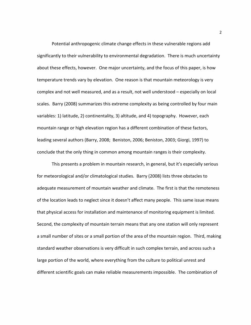
Potential anthropogenic climate change effects in these vulnerable regions add
significantly to their vulnerability to environmental degradation. There is much uncertainty
about these effects, however. One major uncertainty, and the focus of this paper, is how
temperature trends vary by elevation. One reason is that mountain meteorology is very
complex and not well measured, and as a result, not well understood – especially on local
scales. Barry (2008) summarizes this extreme complexity as being controlled by four main
variables: 1) latitude, 2) continentality, 3) altitude, and 4) topography. However, each
mountain range or high elevation region has a different combination of these factors,
leading several authors (Barry, 2008; Beniston, 2006; Beniston, 2003; Giorgi, 1997) to
conclude that the only thing in common among mountain ranges is their complexity.
This presents a problem in mountain research, in general, but it’s especially serious
for meteorological and/or climatological studies. Barry (2008) lists three obstacles to
adequate measurement of mountain weather and climate. The first is that the remoteness
of the location leads to neglect since it doesn’t affect many people. This same issue means
that physical access for installation and maintenance of monitoring equipment is limited.
Second, the complexity of mountain terrain means that any one station will only represent
a small number of sites or a small portion of the area of the mountain region. Third, making
standard weather observations is very difficult in such complex terrain, and across such a
large portion of the world, where everything from the culture to political unrest and
different scientific goals can make reliable measurements impossible. The combination of

3
these issues means that, in order to get complete measurements of mountain systems
around the world, a very large number of stations would need to be set up and maintained.
Because of these issues, there is a lack of observational studies of the variation in
climate trends with elevation and across complex terrain. Most studies have focused on
European mountain chains with limited work on western North America, where climatic
change is strongly impacting ecosystems. Here, terrain-‐specific interpolated meteorology
and a digital elevation model (DEM) are used to make statistical inference on the
magnitudes of these trends and the spatial extent and coherence of elevation specific
trends in the western United States.
2. Background
2.1 Topoclimate/Microclimate Although it is beyond the scope of this paper to present a complete, detailed
description of the specific factors which contribute to the complexity of mountain
meteorology, a brief overview is helpful as part of the motivation for this study. The
limitations experienced in observing mountain meteorology have led to the development of
several downscaling techniques specifically designed to interpolate observed and/or
modeled data to a higher resolution in order to capture the very complex and rapidly
changing temperature, precipitation, wind, humidity, radiation, and other meteorological
variables which exist in mountainous regions (or ‘complex terrain’). The goal of this
downscaling is to capture the ‘topoclimates’ which exist in complex terrain. These very high
gradients of climate are a major contributor to the large biodiversity and endemism (species

4
are unique to a particular location) found in mountainous regions. These small scale regions
(~100m to 10 km) exist within the larger scale mountain environment and are mostly
controlled by different amounts of radiation received because of the greatly varying
exposures, facet directions, slope angles, sunlight totals, etc. Further, ‘microclimates’
(~1cm to 100m) exist within these topoclimates (Barry, 2008). Some examples of these
include the surface of leaves, the forest canopy, a clearing, areas near a waterfall or a cave
entrance, a small rock outcrop, and different soil layers. These microclimates have the
largest gradients, and are often a result of the more intense radiation at high altitudes,
which can heat a surface to a temperature much higher than that of the surrounding air
(Barry, 2008). As will be discussed in greater detail later, no downscaling technique, in and
of itself, can accurately and consistently reproduce these topoclimates or microclimates.
Knowledge about the specific geographic and climatic characteristics of the local area is
needed. This fact appears to greatly limit the resolution at which downscaling techniques
can be used, as well as the spatial extent of very high resolution downscaling projects
because the knowledge base needed in such cases is not readily available.
These dramatic differences in surface heating produce very complex wind patterns,
which are then modified further by forests, ridges, valleys, clearings, glaciers, urban
development, agriculture, and other topological and ecological features. For example,
differences in heating between glaciers and surroundings produce ‘glacier winds’, while
sheltered valleys commonly experience cold air pooling at nighttime (Barry, 2008;
Lundquist, 2008; Pepin, Daly, and Lundquist – poster). Synoptic conditions, including
5
regional scale wind strength and direction, cloudiness, and precipitation, must favor the
development of these cold pools, which are often very shallow and local, and not always
recorded by local observation stations. Other winds associated with complex terrain
include the Chinook of the Rocky Mountains, the Santa Ana of California, the fohn and bora
of the Alps, and the katabatic winds of Greenland and Antarctica. Much more detailed
information on topoclimates and microclimates can be found in Barry (2008), Bonan (2008),
de Jong (2005), and Whiteman (2000).
2.2 Literature Review
2.2.1 Previous Studies on Climatic Trends in Mountainous Regions The question of whether or not elevation plays a role in temperature trends is a
relatively new one, which is driven largely by the interest in climate change and its potential
impacts. Most literature on this topic is less than twenty years old, and the pace of this
research seems to be increasing in response to the demand for information on climate
change impacts from policymakers, renewable energy companies, etc. Additionally, a
significant amount of information on temperature trends in mountainous regions can be
retrieved from studies which do not have these trends as their focus. These are not
reviewed here, for the most part. There are also a growing number of conferences around
the world which focus on mountain ecology and climate change, and a significant portion of
this literature review comes from presentations of new, unpublished research given by
some of the leaders in mountain meteorology, ecology, and downscaling research.

6
Just as the topoclimates and microclimates of mountain ranges around the world
cannot be generalized, neither can their temperature trends or their variation by elevation.
Additionally, Seidel and Free (2003) indicate that temperature trends on diurnal, seasonal,
interannual, and multidecadal time scales differ greatly over short distances in complex
terrain. They also point out that determining local trends requires local observations, which
are not available for many locations around the world. According to Barry (1992), the Alps
are, by far, the best studied mountain range in the world. The data used in these studies
varies greatly, depending on what is available for a specific location, but includes GHCN
(Global Historical Climate Network) and other station networks, radiosonde data, satellite
data, dynamically modeled data, and statistically downscaled data.
Pepin and Lundquist (2008) report that study results on whether or not elevational
temperature trends are increasing or decreasing do not always agree. Beniston et al. (1997)
and Seidel and Free (2003) come to this same conclusion. However, Diaz and Bradley
(1997), Liu and Chen (2000) and Beniston and Rebetz (1996) found most high elevation sites
to be warming faster than lower elevation sites. Pepin and Lundquist (2008) also list several
studies which found no significant relationship between elevation and trend magnitude,
including Vuille, et al. (2003), Pepin and Seidel (2005), Liu et al. (2006), and You et al. (2008).
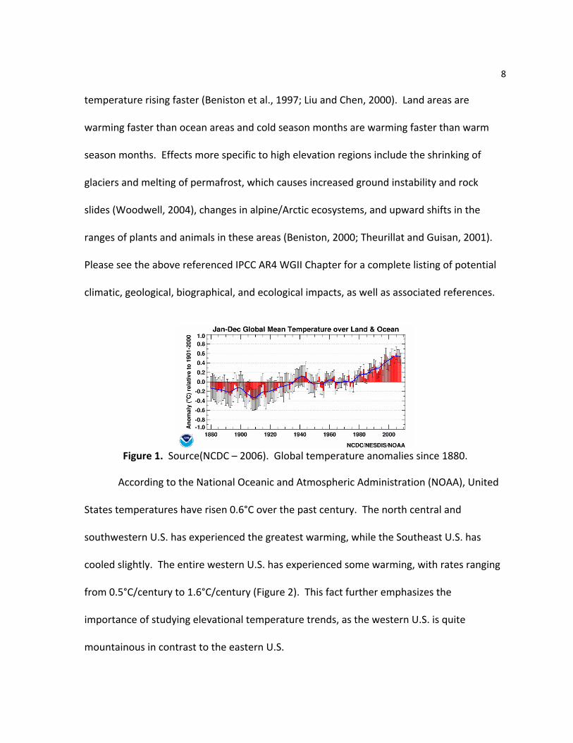
Despite these concerns, Pepin and Lundquist (2008) used GHCN and CRU (Climate
Research Unit) station data to construct a table showing, in general, how temperature
trends vary by elevation throughout the world (Table 1). Their study indicated that areas
near the 0°C isotherm in the extratropics experienced the greatest warming trends due to
7
snow-‐ice feedback effects. Additionally, stations at mountain summits and other locations
where free air drainage/movement (local/regional air flow not impeded by topographic
features) was common showed much more consistent trends, and therefore are
hypothesized to more accurately represent global changes. An important note Pepin and
Lundquist make here is that this consistency is not necessarily due to the notion that
mountain locations may be more sensitive to climate change, but that they are less
influenced by surface complexities, and may provide a good record of Earth’s climate.
Figure 2 shows North American temperature trends by elevation, which form a significant
negative relationship with elevation.
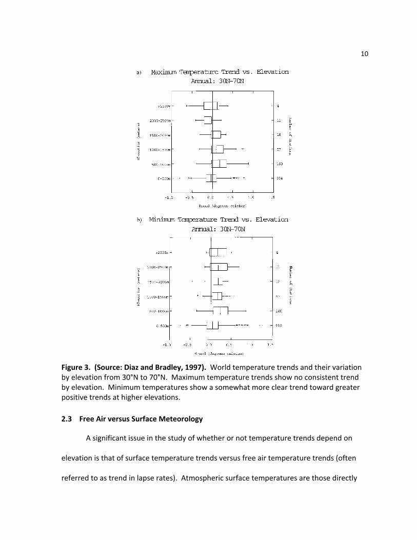
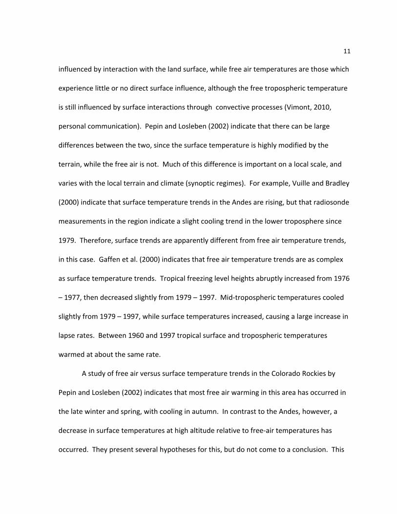
According to Diaz and Bradley (1997), the greatest warming in high elevations has
occurred in Europe and Asia. This same study showed that zonal maximum temperature
trends between 30°N and 70°N do not vary linearly with elevation, while minimum
temperatures show a somewhat more linear, consistent trend toward greater positive trend
magnitudes at higher elevations (Figure 3). Vuille and Bradley (2000) report that trends in
the Andes are greatest at low elevations, but that more recent time periods show trends of
greater positive magnitude at all elevations.
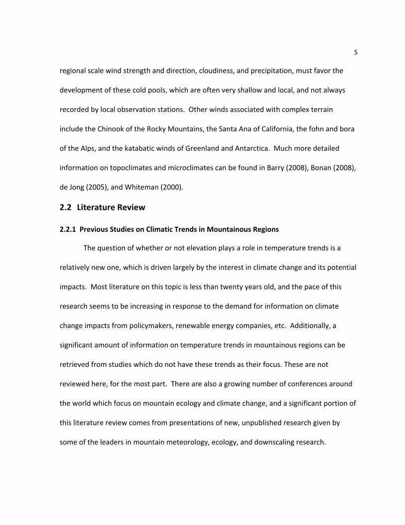
2.2.2 Global and North American Trends Globally, temperatures have risen about 0.8°C over the last century (Figure 1, NCDC –
2006), with current warming rates averaging 1.6°C/century. The 2007 IPCC report (AR4
WGII Chapter 4 -‐ Ecosystems, their Properties, Goods and Services -‐ 4.4.7 Mountains) also
indicates that both minimum and maximum temperatures are rising, with minimum
8
temperature rising faster (Beniston et al., 1997; Liu and Chen, 2000). Land areas are
warming faster than ocean areas and cold season months are warming faster than warm
season months. Effects more specific to high elevation regions include the shrinking of
glaciers and melting of permafrost, which causes increased ground instability and rock
slides (Woodwell, 2004), changes in alpine/Arctic ecosystems, and upward shifts in the
ranges of plants and animals in these areas (Beniston, 2000; Theurillat and Guisan, 2001).
Please see the above referenced IPCC AR4 WGII Chapter for a complete listing of potential
climatic, geological, biographical, and ecological impacts, as well as associated references.
Figure 1. Source(NCDC – 2006). Global temperature anomalies since 1880.
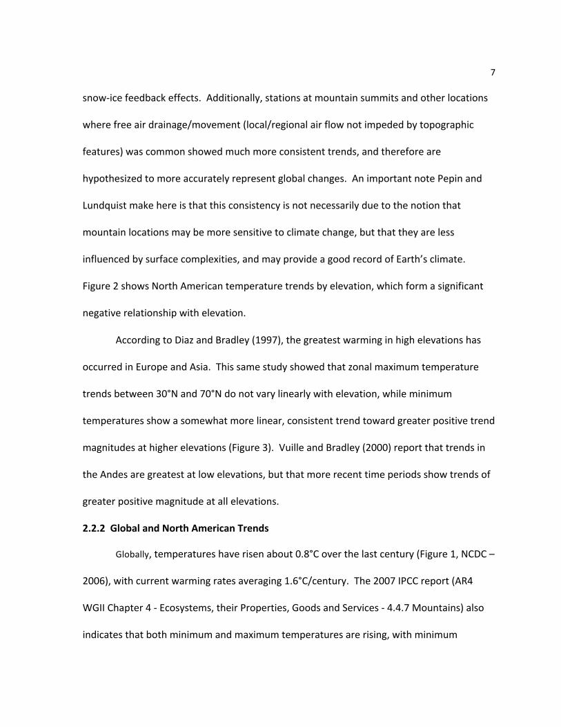
According to the National Oceanic and Atmospheric Administration (NOAA), United
States temperatures have risen 0.6°C over the past century. The north central and
southwestern U.S. has experienced the greatest warming, while the Southeast U.S. has
cooled slightly. The entire western U.S. has experienced some warming, with rates ranging
from 0.5°C/century to 1.6°C/century (Figure 2). This fact further emphasizes the
importance of studying elevational temperature trends, as the western U.S. is quite
mountainous in contrast to the eastern U.S.
9
Figure 2. (Source: NOAA – 2008). Mean annual United States temperature trends from 1901 -‐ 2005. Table 1. (Source: Pepin and Lundquist, 2008). Table showing general temperature trends and their variation by elevation through the world (1948 – 2002). Uncertainty is defined using 95% confidence intervals. Red shading indicates significant warming for the entire continent. Elevation bands were defined by continent by dividing the stations into three equal elevation categories. The North American temperature trend is stronger at lower elevations.
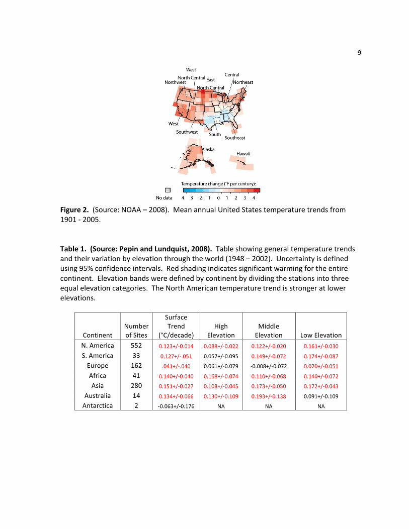
Continent Number of Sites
Surface Trend
(°C/decade) High
Elevation Middle Elevation Low Elevation
N. America 552 0.123+/-‐0.014 0.088+/-‐0.022 0.122+/-‐0.020 0.161+/-‐0.030
S. America 33 0.127+/-‐.051 0.057+/-‐0.095 0.149+/-‐0.072 0.174+/-‐0.087
Europe 162 .041+/-‐.040 0.061+/-‐0.079 -‐0.008+/-‐0.072 0.070+/-‐0.051
Africa 41 0.140+/-‐0.040 0.168+/-‐0.074 0.110+/-‐0.068 0.140+/-‐0.072
Asia 280 0.151+/-‐0.027 0.108+/-‐0.045 0.173+/-‐0.050 0.172+/-‐0.043
Australia 14 0.134+/-‐0.066 0.130+/-‐0.109 0.193+/-‐0.138 0.091+/-‐0.109
Antarctica 2 -‐0.063+/-‐0.176 NA NA NA
10
Figure 3. (Source: Diaz and Bradley, 1997). World temperature trends and their variation by elevation from 30°N to 70°N. Maximum temperature trends show no consistent trend by elevation. Minimum temperatures show a somewhat more clear trend toward greater positive trends at higher elevations. 2.3 Free Air versus Surface Meteorology
A significant issue in the study of whether or not temperature trends depend on
elevation is that of surface temperature trends versus free air temperature trends (often
referred to as trend in lapse rates). Atmospheric surface temperatures are those directly
11
influenced by interaction with the land surface, while free air temperatures are those which
experience little or no direct surface influence, although the free tropospheric temperature
is still influenced by surface interactions through convective processes (Vimont, 2010,
personal communication). Pepin and Losleben (2002) indicate that there can be large
differences between the two, since the surface temperature is highly modified by the
terrain, while the free air is not. Much of this difference is important on a local scale, and
varies with the local terrain and climate (synoptic regimes). For example, Vuille and Bradley
(2000) indicate that surface temperature trends in the Andes are rising, but that radiosonde
measurements in the region indicate a slight cooling trend in the lower troposphere since
1979. Therefore, surface trends are apparently different from free air temperature trends,
in this case. Gaffen et al. (2000) indicates that free air temperature trends are as complex
as surface temperature trends. Tropical freezing level heights abruptly increased from 1976
– 1977, then decreased slightly from 1979 – 1997. Mid-‐tropospheric temperatures cooled
slightly from 1979 – 1997, while surface temperatures increased, causing a large increase in
lapse rates. Between 1960 and 1997 tropical surface and tropospheric temperatures
warmed at about the same rate.
A study of free air versus surface temperature trends in the Colorado Rockies by
Pepin and Losleben (2002) indicates that most free air warming in this area has occurred in
the late winter and spring, with cooling in autumn. In contrast to the Andes, however, a
decrease in surface temperatures at high altitude relative to free-‐air temperatures has
occurred. They present several hypotheses for this, but do not come to a conclusion. This
12
lack of understanding about the changes in lapse rates, and the apparent contrast in surface
temperature trends vs. free-‐air temperature (surface temperatures warming faster than
upper air temperatures) trends shows the need for significantly more research in this area
(Pepin and Losloben, 2002). Surface trends are the focus of this paper for two reasons: 1)
station data is representative of surface temperatures and 2) ecosystem impacts are
dependent on surface temperatures.
As already stated, much uncertainty exists, even in the studies performed, because
of the scarcity of observational data. The effects of synoptic regime, local terrain, land
cover, free air vs. surface temperatures, ENSO (EL Nino Southern Oscillation), feedbacks,
etc. on climate trends in mountain regions combine to make prediction of climate change
effects very difficult. This has led to using models to predict future climate in these areas.
However, the same variables that contribute to the lack of current observations also
contribute to the difficulty of modeling climate for these regions. Pepin and Lundquist
(2008), however, note that nearly all global climate models produce too strong a warming
feedback at high elevations (above the 0°C isotherm), which is likely due to the ice-‐snow
albedo feedback. According to Nogues-‐Bravo et al. (2007), the IPCC expects mountain
ranges to experience 21st century warming rates two to three times higher than those of the
20th century. In accordance with this, isotherms are expected to move upward between
380 and 550 meters in Europe and North America, affecting the range in which plants and
animals can survive.
13
3. OBJECTIVES
3.1 HYPOTHESES Since the literature shows that North American mountain ranges have not been
studied as well as their European counterparts, that existing studies on elevational
influences on temperature trends are, for the most part, not regionally or locally specific,
and observational networks in mountainous regions are relatively sparse, it is clear we do
not understand the influence of elevation on temperature trends or have the high
resolution data needed in order to effectively and fully understand topoclimates in complex
terrain, or the potential effects of climate change in these regions.
Therefore, my main objective in this study is to study elevational temperature trends
in the western United States for specific mountain ranges using a previously validated
downscaled, topographically adjusted climate data set, for two periods – 1941 to 1970 and
1971 -‐ 2000. Are there spatially coherent elevational trends in temperature in mountain
regimes and how do they relate to global patterns? Also, are these spatial patterns and
general trend patterns consistent globally and across North America or is there significant
geographic variability? Thus, this study has two main hypotheses: 1) trends in mean surface
temperature have taken place over the western U.S. since 1941 and these trends are
amplified with increased elevation due to a snow-‐ice albedo feedback and exposure to the
free atmosphere, and 2) different mountain chains in the western U.S. experience
significantly different trend patterns depending on the primary synoptic regime experienced
by each mountain region. Using a high quality interpolated data set, these hypotheses can
14
be tested. Six mountain chains were used in this study, including: 1) Cascades, 2) Sierra
Nevada, 3) Northern Rockies, 4) Middle Rockies, 5) Southern Rockies, and 6) the Wasatch
Range. Figures 33 and 34 in the appendix show mean seasonal temperatures from 1895 –
2009 for all ecoregions.
3.2 STUDY REGIONS
The geographical outlines for each studied mountainous region are based on Bailey’s
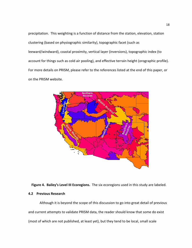
Level III Ecoregions (Bailey, 1983). Figure 4 shows a map of Bailey’s Level III ecoregions,
with the six in this study labeled. These ecoregions are used as the basis for this study
because these regions are based on precipitation amount and pattern throughout each
region, as well as their temperatures and their distribution. Each ecoregion has unique
geological, climatic, and ecological characteristics, which are briefly described below (source
-‐ EPA’s ecoregion website: http://www.epa.gov/wed/pages/ecoregions/level_iii_iv.htm).
The Cascades are composed mostly of volcanoes, both dormant and active.
Glaciation has significantly affected the range, and it is characterized by many steep ridges
and river valleys in the west, and a high plateau in the east. Ranging up to 14,411 feet in
height, it has a moist, temperate climate which supports an extensive and very productive
coniferous forest. Subalpine meadows and rocky alpine zones occur at high elevations. It is
important to note that the Cascade ecoregion stops in central Washington state, and does
not include the North Cascades, which is a distinct and separate ecoregion.
The Sierra Nevada range rises quickly from the dry basin to its east, and slopes
gently toward the central California to its west. The east side has been heavily glaciated

15
and alpine conditions exist at its highest elevations. Vegetation includes ponderosa pine
and douglas-‐fir at low west side elevations, pin and Sierra juniper on its east side, to fir and
other conifers at higher elevations.
The Northern Rockies is a very rugged, strongly glacier influenced, high marine
influenced ecoregion. Although this region is not as high as the Canadian or Southern
Rockies, the highest elevations include alpine characteristics and numerous glacial lakes.
Douglas and subalpine fir, Englemann spruce, ponderosa pine, western red cedar, western
hemlock, and grand fir are common and are indicative of the marine influence.
The Middle Rockies lack the strong maritime influence of the Northern Rockies, and
the lack of Pacific tree species is indicative of this. Douglas and subalpine fir, as well as
Engelmann spruce are common. Large alpine areas are common, as are partly wooded or
shrub and grass covered areas. Intermontane valleys are also grass and/or shrub covered,
containing unique flora and fauna.
The Southern Rockies are high, rugged mountains, comprised of land cover/use
which follows a pattern of elevational banding. Shrub or grass covers the lowest elevations,
while grazing is common at low and middle elevations. Douglas fir, ponderosa pine, aspen,
and juniper-‐oak woodlands are found at low to middle elevations. Coniferous forests cover
the middle to high elevations, which also have alpine characteristics.
The Wasatch Range is also a high, steep mountain chain filled with narrow crests,
valleys, and some plateaus and open mountaintops. Land cover/use follows an elevational
banding pattern similar to that of the Southern Rockies, although aspen, chaparral, juniper-‐
16
pinyon, and scrub oak are found at middle elevations. Summer grazing of livestock is also
common.
Table 2 shows the mean, minimum, and maximum elevation for each range. The
Southern Rockies has the highest mean elevation (2279 meters), while the Cascades have
the lowest (881 meters). All mountain regions have elevation ranges of 2278 meters or
greater, with the Sierra Nevada have the greatest (3936 meters). Additionally, the variety
of mountainous regions allows me to test the potential influence of synoptic regime on
elevational trends.
4. Methodology
4.1 Data Set – PRISM
The main objective of my research is to study temperature trends and their variation
with elevation throughout the western U.S. from 1895 to 2009, with a focus on two periods,
1941 – 1970 and 1971 – 2000. As stated earlier, Pepin and Lundquist have performed a
similar analysis using GHCN, CRU, and NWS data. However, the number of stations at high
elevations in the western U.S. is still less than exists at lower, more populated elevations.
To compensate for this, I use the PRISM (Parameter-‐Regressions on Independent Slopes
Model) data set developed by Dr. Christopher Daly at Oregon State University (Daly, et al.
2008). This data set uses an advanced downscaling scheme to interpolate observed
maximum and minimum temperature, precipitation, and dew point temperature to a 4 km
grid across the conterminous U.S. on a monthly time scale from 1895 to the current month
(Note: An 800m dataset is available, but I used the 4 km data set). The PRISM website
17
(http://www.prism.oregonstate.edu/docs/index.phtml) contains many publications,
presentations, and posters which describe PRISM’s interpolation scheme in detail. These
are listed in this paper’s reference section. I will summarize the algorithm here.
The PRISM model was developed mainly for interpolating temperature and
precipitation in complex terrain. Therefore, elevation is the main variable in the algorithm,
which uses several unique methods to accurately model its effect on temperature on a
monthly time scale.
The first of these methods is that PRISM uses a knowledge base to “inject knowledge
into a climate mapping system” (PRISM overview – presentation, 2008). This knowledge
base includes several factors, with the main one being the fact that precipitation increases
and temperature decreases with elevation, and that this relationship is often linear. This
computer based system automatically makes decisions based on this knowledge base.
Other factors in this knowledge base include terrain induced climate transitions
(topographic facets and a ‘moisture index’ or moisture regime – including windward vs
leeward sides of a mountain range), coastal effects due to proximity, a two layer
atmosphere and a topographic index (allows for temperature inversions), orographic
effectiveness of terrain (at lifting the air -‐ based on topographical steepness and
orientation, wind direction), and persistence of climate patterns.
The second part of the algorithm, and the mathematical basis of the model, is a
moving window regression of climate vs. elevation for each grid cell. The third part of the
algorithm is the station weighting used to produce the monthly temperature or
18
precipitation. This weighting is a function of distance from the station, elevation, station
clustering (based on physiographic similarity), topographic facet (such as
leeward/windward), coastal proximity, vertical layer (inversions), topographic index (to
account for things such as cold air pooling), and effective terrain height (orographic profile).
For more details on PRISM, please refer to the references listed at the end of this paper, or
on the PRISM website.
Figure 4. Bailey’s Level III Ecoregions. The six ecoregions used in this study are labeled.
4.2 Previous Research
Although it is beyond the scope of this discussion to go into great detail of previous
and current attempts to validate PRISM data, the reader should know that some do exist
(most of which are not published, at least yet), but they tend to be local, small scale
19
projects that do not represent the fact that PRISM’s interpolation represents the average
temperature over a 16km2 area. However, Scully (2010) did a nationwide study similar to
that of section 5.3.2, by ecoregion (7474 stations used, plus 712 SNOTEL stations, 1980 -‐
2003). Although this study’s goal was to compare PRISM and Daymet (Thornton et al.
1997), much of the work performed is applicable to this study. I will present here what I
feel are the most relevant results.
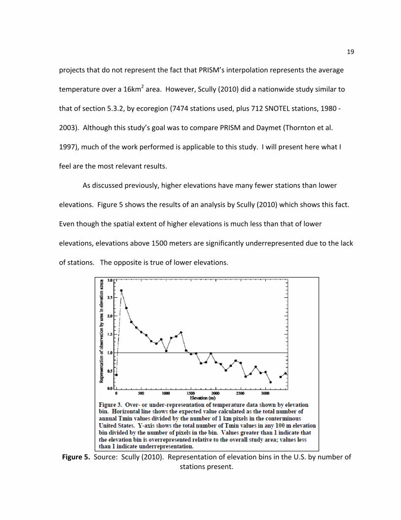
As discussed previously, higher elevations have many fewer stations than lower
elevations. Figure 5 shows the results of an analysis by Scully (2010) which shows this fact.
Even though the spatial extent of higher elevations is much less than that of lower
elevations, elevations above 1500 meters are significantly underrepresented due to the lack
of stations. The opposite is true of lower elevations.
Figure 5. Source: Scully (2010). Representation of elevation bins in the U.S. by number of
stations present.
20
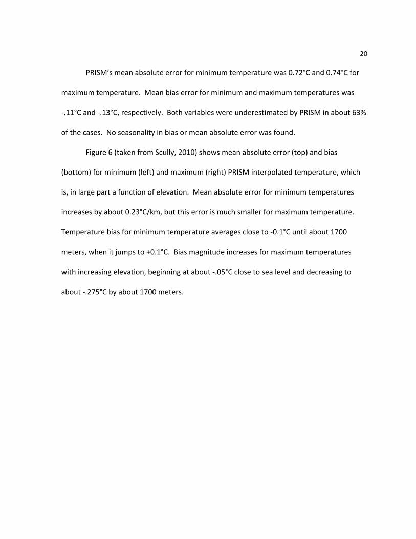
PRISM’s mean absolute error for minimum temperature was 0.72°C and 0.74°C for
maximum temperature. Mean bias error for minimum and maximum temperatures was
-‐.11°C and -‐.13°C, respectively. Both variables were underestimated by PRISM in about 63%
of the cases. No seasonality in bias or mean absolute error was found.
Figure 6 (taken from Scully, 2010) shows mean absolute error (top) and bias
(bottom) for minimum (left) and maximum (right) PRISM interpolated temperature, which
is, in large part a function of elevation. Mean absolute error for minimum temperatures
increases by about 0.23°C/km, but this error is much smaller for maximum temperature.
Temperature bias for minimum temperature averages close to -‐0.1°C until about 1700
meters, when it jumps to +0.1°C. Bias magnitude increases for maximum temperatures
with increasing elevation, beginning at about -‐.05°C close to sea level and decreasing to
about -‐.275°C by about 1700 meters.
21
Figure 6. Source: Scully (2010). PRISM mean absolute error and temperature bias for minimum and maximum temperatures. Both error and bias increase at greater elevations, which is expected because fewer stations exist in high elevations, and the more complex topography creates higher temperature gradients in these areas.
TMin
TMax
22
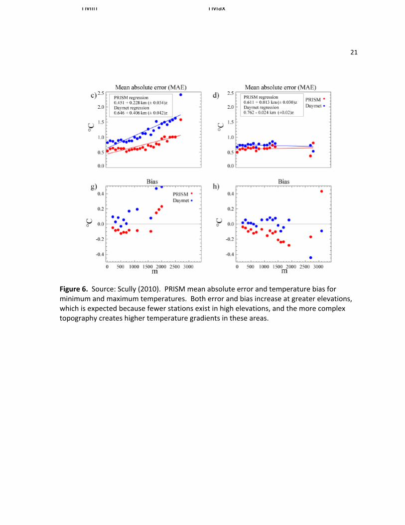
4.3 Definition of Mountainous Regions Although the ecoregions are used as the basis for each of the mountainous areas in
this study, I used a buffer of approximately 50km around each ecoregion for the elevational
analysis. There are two reasons for this. One, in many cases, Bailey’s ecoregions closely
follow a particular elevation contour. This means that choosing the exact boundaries of the
ecoregion would significantly limit the elevational range of the analysis for each region.
Also, the number of stations at high locations is limited, so choosing a larger area allows for
the inclusion of more station data. These buffers were created using IDRISI Taiga.
Table 2. Buffered Elevational and Area Statistics.
Region
Mean Elevation
(m)
Minimum Elevation
(m)
Maximum Elevation
(m)
Elevation Range (m)
Std. Dev. (m)
Area (Km2)
Cascades 881.7 23 3255 3232 517.5 76194.7 Sierra Nevada 1417.3 9 3945 3936 855.3 133754.2
Northern Rockies 1128.2 240 2518 2278 386.7 116043.6 Middle Rockies 1997.2 800 3781 2981 482.6 253857.0 Southern Rockies 2279.9 1283 4005 2722 526.2 313946.3 Wasatch Range 2063.7 889 3711 2822 461.2 125150.4
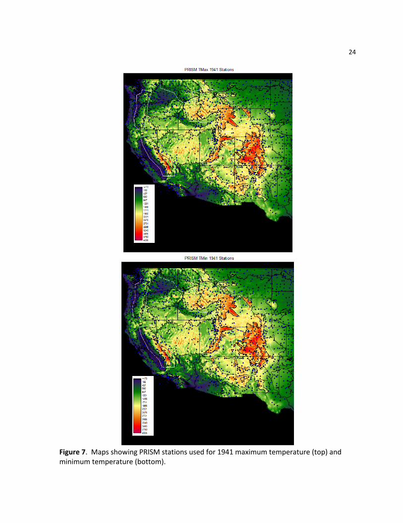
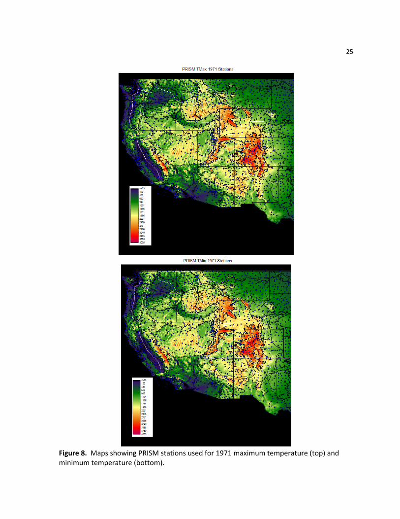
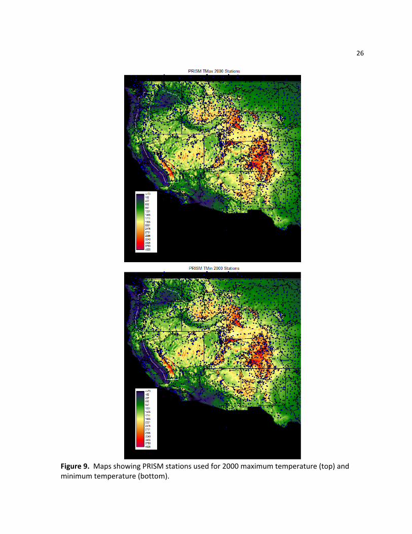
Figures 7 -‐ 9 show the stations used in the PRISM model, with the PRISM digital
elevation model (DEM) overlaid, and the ecoregions and states outlined in black. The areas
outlined in white indicate the buffered areas around each ecoregion used in the elevational
trend analysis. Table 2 provides detailed information about each buffered area (outlined in
white). The distribution of stations the PRISM model uses in its downscaling algorithm for
1941, 1971, and 2000 is shown in these figures (these are the beginning and end years of
the periods of study). More stations are available, in general, as time progresses.
Additionally, the distribution of these stations is quite good, even across the highest

23
elevations. The one exception to this tends to be the Sierra Nevada, especially across its
southern portions. Eastern portions of the Wasatch and southeastern portions of the
Middle Rockies also show sparse station locations for 1941 and 1971, with a dramatic
increase in station coverage in 2000. Additionally, low elevations at the foothills of the
ranges tend to have a concentration of stations (such as the western parts of the Sierra
Nevada and Wasatch Range, and the front range of the Southern Rockies.
24
Figure 7. Maps showing PRISM stations used for 1941 maximum temperature (top) and minimum temperature (bottom).
25
Figure 8. Maps showing PRISM stations used for 1971 maximum temperature (top) and minimum temperature (bottom).
26
Figure 9. Maps showing PRISM stations used for 2000 maximum temperature (top) and minimum temperature (bottom).
27
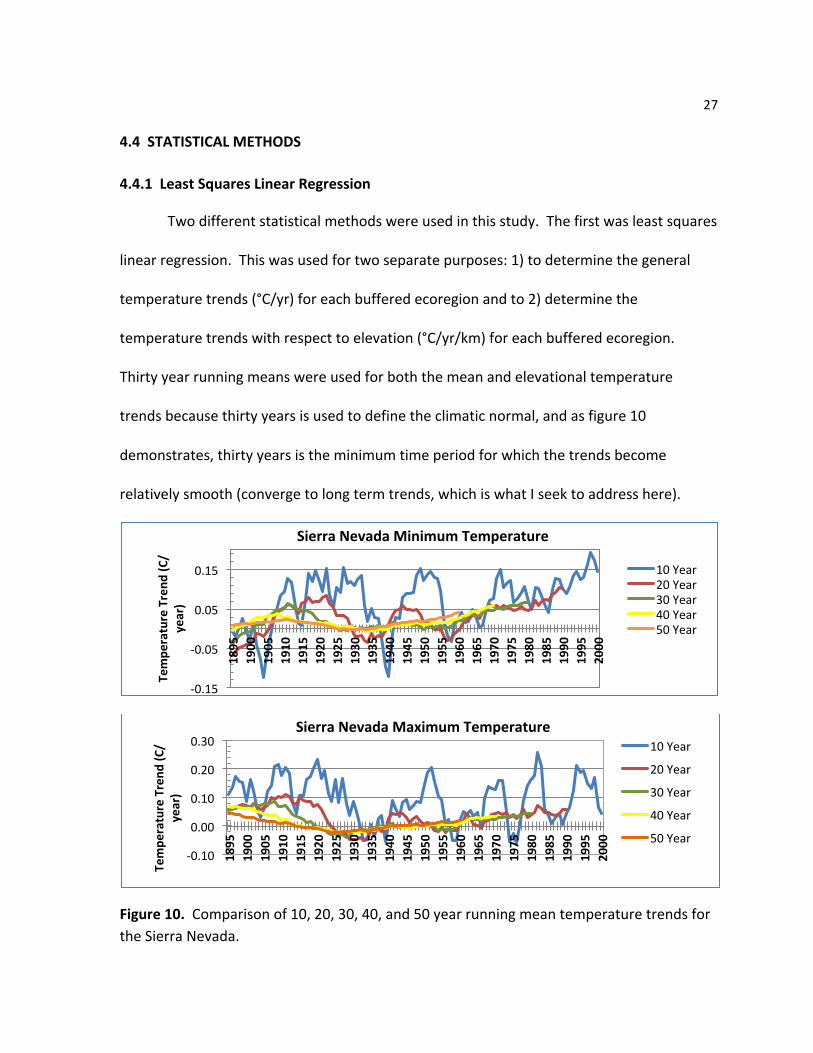
4.4 STATISTICAL METHODS 4.4.1 Least Squares Linear Regression Two different statistical methods were used in this study. The first was least squares
linear regression. This was used for two separate purposes: 1) to determine the general
temperature trends (°C/yr) for each buffered ecoregion and to 2) determine the
temperature trends with respect to elevation (°C/yr/km) for each buffered ecoregion.
Thirty year running means were used for both the mean and elevational temperature
trends because thirty years is used to define the climatic normal, and as figure 10
demonstrates, thirty years is the minimum time period for which the trends become
relatively smooth (converge to long term trends, which is what I seek to address here).
Figure 10. Comparison of 10, 20, 30, 40, and 50 year running mean temperature trends for the Sierra Nevada.
-‐0.15
-‐0.05
0.05
0.15
1895
1900
1905
1910
1915
1920
1925
1930
1935
1940
1945
1950
1955
1960
1965
1970
1975
1980
1985
1990
1995
2000
Tempe
rature Trend
(C/
year)
Sierra Nevada Minimum Temperature
10 Year 20 Year 30 Year 40 Year 50 Year
-‐0.10
0.00
0.10
0.20
0.30
1895
1900
1905
1910
1915
1920
1925
1930
1935
1940
1945
1950
1955
1960
1965
1970
1975
1980
1985
1990
1995
2000
Tempe
rature Trend
(C/
year)
Sierra Nevada Maximum Temperature 10 Year
20 Year
30 Year
40 Year
50 Year
28
4.4.2 K-‐Means Cluster Analysis
The second statistical method used was k-‐means cluster analysis. This method is
very useful because it determines how to best group data observations while maintaining
consistency in seasonal trends. For this analysis, 30 year running trends for minimum and
maximum temperature, precipitation, and dew point for each season and each grid cell, for
the entire western U.S., were clustered. Two separate analyses were performed. One
analyses used each season separately (4 variables) and the other used the four variables for
all seasons (16 variables). Each four variable clustering analysis (one per season) produced
different elevation means and different temperature trends for each cluster centroid. The
centroid of a cluster represents the multidimensional ‘center’ for the observations of the
variables used in the analysis. Each sixteen variable analysis produced one elevation mean
for all seasons (a yearly average) and four different seasonal mean temperatures for each
elevation mean (and cluster centroid value). The result was a grouping of the trends into
regions for these four variables for each season for both periods, 1941 – 1970 and 1971 –
2000.
There are many variations within the general k-‐means method, so it is important to
discuss the specific steps used for this analysis (Bradley, et al. (1997). First, the observations
for minimum and maximum temperature, precipitation, and dew point trends were
normalized. As a result, the clustering operates on the variance of the data set. The entire
data set is first randomly divided into ten separate groups of equal size (each of which is
assumed to be representative of the entire data set). Within each of these ten groups, each

29
observation is assigned to one of k seeds, or randomly placed locations (values of the
normalized variables) within the multidimensional space of the analysis. This yields ten
different versions for the locations of the k seeds. The version with the lowest Euclidean
distance (variance) between seeds and observations is used as the initial step for the next
step. This method is used because k-‐means cluster analysis is very sensitive to the initial
seeds used, and this method makes it likely that, if the analyses is repeated, the same
answer will emerge.
Next, all observations are assigned to the nearest seed location as determined from
the first step, and the total Euclidean distance is calculated. Then, the observations furthest
from the centroids are reassigned to the nearest neighbor centroids, the centroid values are
recomputed, and the total variance is recalculated. This process continues until the number
of observations which are reassigned is less than 0.5% of the total.
The best number of clusters was determined to be fifty, based on the fact that the
sum of the squared error (of the Euclidean distance) leveled out at an approximate
minimum of fifty clusters in all cases. This method was used because it does not take into
account or assume any prior knowledge about the data set before attempting to divide the
data into clusters (often referred to as machine learning or a form of data mining). Finally,
the mean elevation was calculated for each cluster, based on the location and the elevation
the PRISM DEM assigned for each grid cell contained in the cluster.
Although this method was used because it produces robust results, it does not
provide any information about which variable is most important. In this study, it only
30
provides information about trend similarity among PRISM grid cells. Dr. Bjorn Brooks of the
University of Wisconsin Madison provided sample clustering programs which were adapted
for the study during Spring and Fall 2010. Tables 6 – 9 in the appendix provide specific
cluster statistics for the period 1971 – 2000 for elevation, as well as minimum and
maximum temperature. Figures 33 and 34 are example maps showing the mean spring
cluster trends for all 50 clusters for both 1941 – 1970 and 1971 – 2000. Note that the mean
cluster value for both variables increases from the early period to the later period. Also,
clusters are spatially much more complex in the mountain regions as compared to the
plains. In some cases, significant differences occur, including clusters with means trends of
opposite signs, in adjacent clusters.
For both periods, clustering for the early period tends to show a clear spatial pattern
where clusters with greater positive values are located in mountainous areas. The one
exception to this, however, is the Sierra Nevada range, where highly negative mean cluster
trends are present for both periods in the northern 2/3 of the range, while positive values
occur in the southern 1/3. A visual inspection also seems to indicate that mean cluster
trends are more spatially variable in the later period, which may be a reflection of fewer
stations in this ecoregion than in other ecoregions.
5. Results
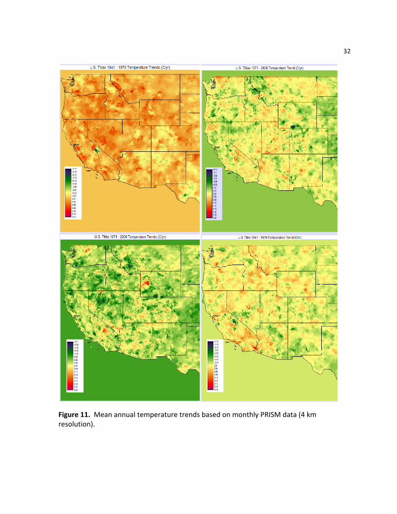
5.1. Mean Seasonal Temperature Trends As shown in Figure 11, maximum and minimum temperature trends over the
western United States for the periods 1941 – 1970 and 1971 – 2000 are highly spatially
31
variable. This variation is largely due to the interaction of the complex terrain with the local
synoptic regime, its continentality, and other factors, which are poorly understood. Based
solely on temperature trends over these two periods, it is rather difficult to discern terrain
influenced trends. Some basic patterns can be seen, however. The Colorado Rockies
(Southern Rockies) have generally higher or positive trends during all periods, except for
1941 – 1970 maximum temperature, for which the trends are slightly negative. The central
valley of California can be seen as a long oval bordered by generally higher, positive trends
to its east, especially for the later period. Later period maximum trends show the Wasatch
Range in Utah, while minimum trends for the same period are similar throughout the
Cascade Range. The mountain/valley terrain of Nevada can also be seen, especially for
1971-‐ 2000. Otherwise, the trends are generally of greater magnitude for minimum
temperatures than for maximum temperatures, which is consistent with global temperature
trends. An important note here is that some spatial anomalies in the trends do occur. In
particular, an area of highly negative trends is present in the central Sierra Nevada for 1941
– 1970 and in south central Wyoming (not in any ecoregion – but part of this region is
included in the buffered Wasatch Range and Southern Rockies regions used in the
elevational trend analysis). I did not determine whether these anomalies are due to station
data or actual terrain influences, although they appear to be caused by station data because
neither anomaly is present for both time periods.
32
Figure 11. Mean annual temperature trends based on monthly PRISM data (4 km resolution).

33
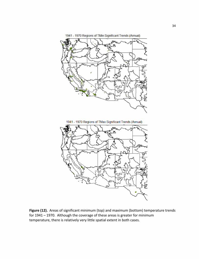
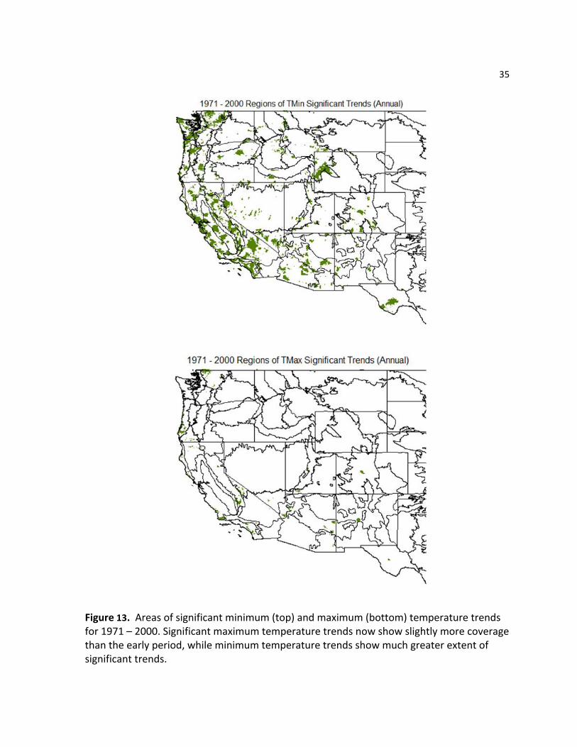
Figures 12 and 13 show where minimum and maximum annual temperature trends
for both periods are statistically significant. Here, a statistically significant trend is based on
whether or not the slope of the best fit least squares regression line is different from zero
(no slope). In this case, the degrees of freedom were based on the number of time series
points (30 years of monthly data). Trends for maximum temperature during the early
period show virtually no significance across the western U.S., except for a small area on the
southeast border of the Sierra Nevada ecoregion. For the later period, the areal spatial
extent of significant trends expand slightly, including parts of the Pacific Northwest,
California, and a few small portions of the interior western U.S. Minimum temperature
trends for the early period are also significant across parts of the Pacific Northwest and
California. By far, the largest portion of significant trends are present for later period
minimum temperatures. Once again, the Pacific Northwest and California contain most of
the significant trends. However, some portions of the Middle and Southern Rockies contain
significant trends. Many smaller areas of significant trends are scattered throughout the
entire region.
34
Figure (12). Areas of significant minimum (top) and maximum (bottom) temperature trends for 1941 – 1970. Although the coverage of these areas is greater for minimum temperature, there is relatively very little spatial extent in both cases.
35
Figure 13. Areas of significant minimum (top) and maximum (bottom) temperature trends for 1971 – 2000. Significant maximum temperature trends now show slightly more coverage than the early period, while minimum temperature trends show much greater extent of significant trends.
36
The mean seasonal temperature trends for the six mountain ranges in this study
share some very general characteristics. Mean seasonal maximum temperature trends are
more variable throughout the study period than the minimum trends, which tend to be
more consistent and follow a trend closer to zero. Each range shows relatively high trends
through the 1920’s, after which they level off or decrease to the mid or late 20th century,
and then begin a rise. Additionally, seasonal trends for each range tend to share general
trends, although some important differences are apparent.
In spite of these similarities, each range has its own unique seasonal temperature
trend patterns. As shown in figures 14 – 19, these patterns are quite complex.
Interestingly, each season’s trends are highly variable, and no single season is more
consistent or less variable than another across the different ranges.
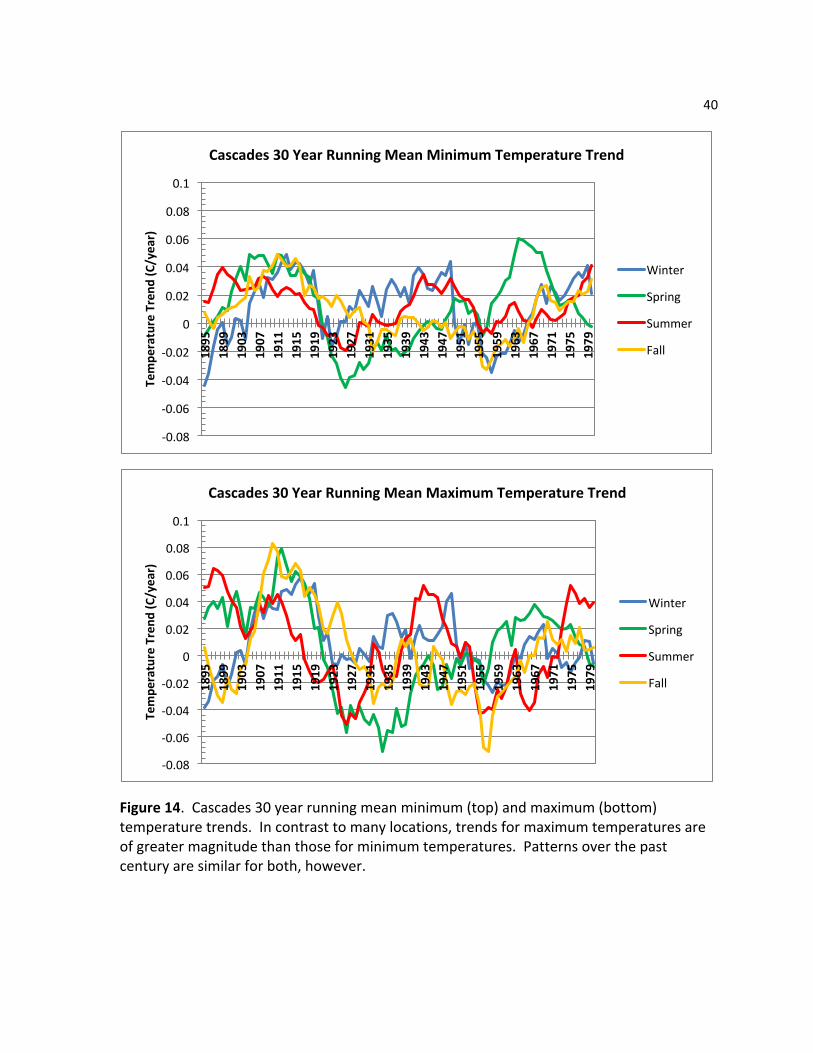
The Cascades show peaks for both minimum and maximum trends around 1910,
1945, and 1965, with minimum trends occurring around 1925 and 1955. Spring minimum
trends peak close 0.06°C/year around 1965, while the other seasons experience very little
or no trend. Trends for the other months then increase, while the spring trend decreases to
zero. In contrast to minimum trends, maximum recent trends for the Cascades occur during
summer, while the other seasons trends remain near zero. Additionally, the Cascades are
currently experiencing the smallest mean seasonal trend magnitudes of any range.
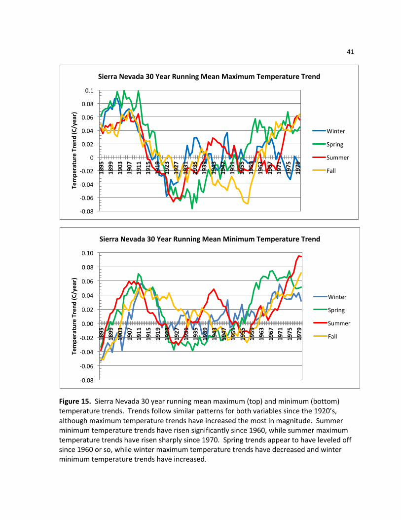
Minimum trends for the Sierra Nevada show a very large range since 1895. Trends
rose to between 0.6°C and 1.0°C/year before 1910, and then fell to around -‐0.06°C/yr by
1927. Since then, all seasons, except winter, have experienced a moderate rate of increase
37
to between 0.04 and 0.06°C/yr. Winter’s minimum trend remains near zero. The spring
minimum trend has appeared to have leveled off since 1960, while fall’s trend has risen
sharply since 1957. Maximum trends, on the other hand, peaked for all seasons around
1912, fell to a mean of around zero by 1930 and have risen quickly since 1960. The spring
maximum trend has also appeared to have peaked already and is now steady at about
0.05°C/yr.
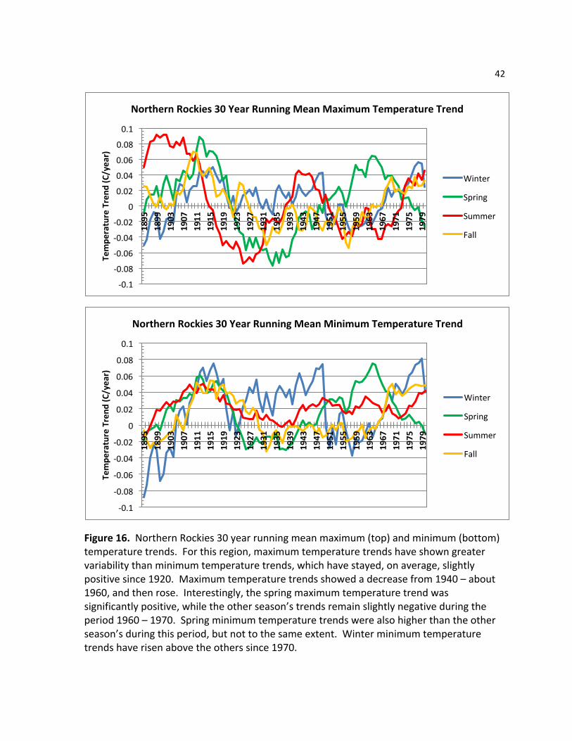
After peaking around 1910, mean maximum temperature trends for the Northern
Rockies for spring and summer fell to a minimum around 1937, rose to another peak about
1943, and are currently experiencing a peak. The fall and winter minimum trends for this
region have been significantly less variable, although they follow a similar pattern. Winter
maximum trends have been the most variable, on the other hand, and have mostly been
above zero since 1895. Summer trends have been small, but entirely positive during this
period, and fall trends remained close to zero through 1965, and then rose. Spring trends
for both variables peaked around 1965 and have since fallen to slightly negative.
In similar fashion to the Northern Rockies, both minimum and maximum trends for
spring in the Middle Rockies peaked around 1965, and have since fallen, although they
remain above zero in this region. Maximum winter and fall trends are the least variable,
while both spring and summer trends experienced a relatively large minimum during the
1920 and 1930’s. Except for winter, all maximum trends are still rising. Minimum trends for
fall and summer are the least variable and are still rising, while winter trends peaked during

38
the 1930’s, fell to slightly negative values around 1960 and then rose very quickly to their
current peak.
Both minimum and maximum seasonal trends in the Southern Rockies are quite
coherent, with little variation between seasons. Maximum trends show a large peak around
1915, a drop to around zero by 1950 (except fall, which fell to -‐0.06°C/yr), and then rapidly
rise. Spring trends appear to have leveled off recently, while winter trends have dropped
very recently. Minimum trends show a small peak around 1915, a long period of trends
close to zero from 1920 – 1955, and then a rapid rise of all seasonal trends. Once again,
spring trends appear to have leveled off since around 1963.
Maximum trends in the Wasatch Range are very close to the Southern Rockies
minimum trends. Spring trends appear to have leveled off in similar fashion, although the
other seasons trends continue to rise and have surpassed that of spring. Minimum trends
were quite consistent during the earlier part of the 20th century. Maximum trends
experienced a larger peak around 1910, fell to near zero by 1920 and stayed there through
1960, after which they rose. Spring shows the highest trend, however, in contrast to the
other seasons, which follow each other very closely.
Table 3 summarizes the mean seasonal temperature trends for each ecoregion for
1941 – 1970 and 1971 – 2000. All trends that were found to be significant are positive,
which was not expected for the early period, since many locations around the world,
including portions of North America, experienced no trend or even slight cooling during this
period (Figure 1). These results are representative of local rates of change, therefore. All
39
significant trends are for minimum temperatures, except for 1971 – 2000 maximum trends
for the Wasatch. The number of significant trends increased nearly threefold over the two
periods, as well. Winter, spring, and fall are the most common seasons showing significant
trends. A bias toward southern regions having more significant trends is evident, with the
Sierra Nevada, Middle Rockies, and Wasatch holding the most significant trends for the later
period. Interestingly, these same ranges showed significant summer trends during the early
period, but these were not present for the later period. However, the only significant trend
for the Southern Rockies for both periods is the summer trend. The Northern Rockies were
expected to show more significant trends, especially for the later period, because of their
relatively high latitude. However, they are also the lowest in elevation. This is not a tested
hypothesis in this paper, but perhaps this moderates their general temperature trends.
40
Figure 14. Cascades 30 year running mean minimum (top) and maximum (bottom) temperature trends. In contrast to many locations, trends for maximum temperatures are of greater magnitude than those for minimum temperatures. Patterns over the past century are similar for both, however.
-‐0.08
-‐0.06
-‐0.04
-‐0.02
0
0.02
0.04
0.06
0.08
0.1
1895
1899
1903
1907
1911
1915
1919
1923
1927
1931
1935
1939
1943
1947
1951
1955
1959
1963
1967
1971
1975
1979
Tempe
rature Trend
(C/year)
Cascades 30 Year Running Mean Minimum Temperature Trend
Winter
Spring
Summer
Fall
-‐0.08
-‐0.06
-‐0.04
-‐0.02
0
0.02
0.04
0.06
0.08
0.1
1895
1899
1903
1907
1911
1915
1919
1923
1927
1931
1935
1939
1943
1947
1951
1955
1959
1963
1967
1971
1975
1979
Tempe
rature Trend
(C/year)
Cascades 30 Year Running Mean Maximum Temperature Trend
Winter
Spring
Summer
Fall
41
Figure 15. Sierra Nevada 30 year running mean maximum (top) and minimum (bottom) temperature trends. Trends follow similar patterns for both variables since the 1920’s, although maximum temperature trends have increased the most in magnitude. Summer minimum temperature trends have risen significantly since 1960, while summer maximum temperature trends have risen sharply since 1970. Spring trends appear to have leveled off since 1960 or so, while winter maximum temperature trends have decreased and winter minimum temperature trends have increased.
-‐0.08
-‐0.06
-‐0.04
-‐0.02
0
0.02
0.04
0.06
0.08
0.1
1895
1899
1903
1907
1911
1915
1919
1923
1927
1931
1935
1939
1943
1947
1951
1955
1959
1963
1967
1971
1975
1979
Tempe
rature Trend
(C/year)
Sierra Nevada 30 Year Running Mean Maximum Temperature Trend
Winter
Spring
Summer
Fall
-‐0.08
-‐0.06
-‐0.04
-‐0.02
0.00
0.02
0.04
0.06
0.08
0.10
1895
1899
1903
1907
1911
1915
1919
1923
1927
1931
1935
1939
1943
1947
1951
1955
1959
1963
1967
1971
1975
1979
Tempe
rature Trend
(C/year)
Sierra Nevada 30 Year Running Mean Minimum Temperature Trend
Winter
Spring
Summer
Fall
42
Figure 16. Northern Rockies 30 year running mean maximum (top) and minimum (bottom) temperature trends. For this region, maximum temperature trends have shown greater variability than minimum temperature trends, which have stayed, on average, slightly positive since 1920. Maximum temperature trends showed a decrease from 1940 – about 1960, and then rose. Interestingly, the spring maximum temperature trend was significantly positive, while the other season’s trends remain slightly negative during the period 1960 – 1970. Spring minimum temperature trends were also higher than the other season’s during this period, but not to the same extent. Winter minimum temperature trends have risen above the others since 1970.
-‐0.1
-‐0.08
-‐0.06
-‐0.04
-‐0.02
0
0.02
0.04
0.06
0.08
0.1
1895
1899
1903
1907
1911
1915
1919
1923
1927
1931
1935
1939
1943
1947
1951
1955
1959
1963
1967
1971
1975
1979
Tempe
rature Trend
(C/year)
Northern Rockies 30 Year Running Mean Maximum Temperature Trend
Winter
Spring
Summer
Fall
-‐0.1
-‐0.08
-‐0.06
-‐0.04
-‐0.02
0
0.02
0.04
0.06
0.08
0.1
1895
1899
1903
1907
1911
1915
1919
1923
1927
1931
1935
1939
1943
1947
1951
1955
1959
1963
1967
1971
1975
1979
Tempe
rature Trend
(C/year)
Northern Rockies 30 Year Running Mean Minimum Temperature Trend
Winter
Spring
Summer
Fall
43
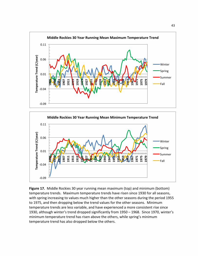
Figure 17. Middle Rockies 30 year running mean maximum (top) and minimum (bottom) temperature trends. Maximum temperature trends have risen since 1930 for all seasons, with spring increasing to values much higher than the other seasons during the period 1955 to 1975, and then dropping below the trend values for the other seasons. Minimum temperature trends are less variable, and have experienced a more consistent rise since 1930, although winter’s trend dropped significantly from 1950 – 1968. Since 1970, winter’s minimum temperature trend has risen above the others, while spring’s minimum temperature trend has also dropped below the others.
-‐0.09
-‐0.04
0.01
0.06
0.11
1895
1899
1903
1907
1911
1915
1919
1923
1927
1931
1935
1939
1943
1947
1951
1955
1959
1963
1967
1971
1975
1979
Tempe
rature Trend
(C/year)
Middle Rockies 30 Year Running Mean Maximum Temperature Trend
Winter
Spring
Summer
Fall
-‐0.09
-‐0.04
0.01
0.06
0.11
1895
1899
1903
1907
1911
1915
1919
1923
1927
1931
1935
1939
1943
1947
1951
1955
1959
1963
1967
1971
1975
1979
Tempe
rature Trend
(C/year)
Middle Rockies 30 Year Running Mean Minimum Temperature Trend
Winter
Spring
Summer
Fall
44
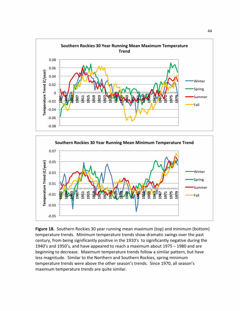
Figure 18. Southern Rockies 30 year running mean maximum (top) and minimum (bottom) temperature trends. Minimum temperature trends show dramatic swings over the past century, from being significantly positive in the 1910’s to significantly negative during the 1940’s and 1950’s, and have appeared to reach a maximum about 1975 – 1980 and are beginning to decrease. Maximum temperature trends follow a similar pattern, but have less magnitude. Similar to the Northern and Southern Rockies, spring minimum temperature trends were above the other season’s trends. Since 1970, all season’s maximum temperature trends are quite similar.
-‐0.08
-‐0.06
-‐0.04
-‐0.02
0
0.02
0.04
0.06
0.08 1895
1899
1903
1907
1911
1915
1919
1923
1927
1931
1935
1939
1943
1947
1951
1955
1959
1963
1967
1971
1975
1979
Tempe
rature Trend
(C/year)
Southern Rockies 30 Year Running Mean Maximum Temperature Trend
Winter
Spring
Summer
Fall
-‐0.05
-‐0.03
-‐0.01
0.01
0.03
0.05
0.07
1895
1899
1903
1907
1911
1915
1919
1923
1927
1931
1935
1939
1943
1947
1951
1955
1959
1963
1967
1971
1975
1979
Tempe
rature Trend
(C/year)
Southern Rockies 30 Year Running Mean Minimum Temperature Trend
Winter
Spring
Summer
Fall
45
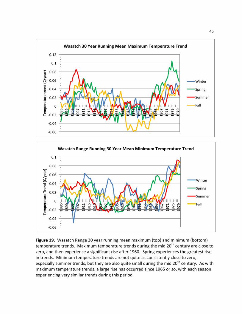
Figure 19. Wasatch Range 30 year running mean maximum (top) and minimum (bottom) temperature trends. Maximum temperature trends during the mid 20th century are close to zero, and then experience a significant rise after 1960. Spring experiences the greatest rise in trends. Minimum temperature trends are not quite as consistently close to zero, especially summer trends, but they are also quite small during the mid 20th century. As with maximum temperature trends, a large rise has occurred since 1965 or so, with each season experiencing very similar trends during this period.
-‐0.06
-‐0.04
-‐0.02
0
0.02
0.04
0.06
0.08
0.1
0.12
1895
1899
1903
1907
1911
1915
1919
1923
1927
1931
1935
1939
1943
1947
1951
1955
1959
1963
1967
1971
1975
1979
Tempe
rature tren
d (C/year)
Wasatch 30 Year Running Mean Maximum Temperature Trend
Winter
Spring
Summer
Fall
-‐0.06
-‐0.04
-‐0.02
0
0.02
0.04
0.06
0.08
0.1
1895
1899
1903
1907
1911
1915
1919
1923
1927
1931
1935
1939
1943
1947
1951
1955
1959
1963
1967
1971
1975
1979
Tempe
rature Trend
(C/year)
Wasatch Range Running 30 Year Mean Minimum Temperature Trend
Winter
Spring
Summer
Fall

46
Table 3. Table showing time period, season, and location of significant trends in mean ecoregion temperature. All significant trends are positive. As expected, the period 1971 – 2000 shows a large increase in the number of significant trends. All significant trends are for minimum temperature, except for the 1971 – 2000 spring Wasatch Range maximum temperature trend.
1941 -‐
1970
1971 -‐
2000
1941 -‐
1970
1971 -‐
2000
Cascades
Winter Tmax
Sierra Nevada
Winter Tmax
Tmin Tmin +
Spring Tmax
Spring Tmax
Tmin Tmin +
Summer Tmax
Summer Tmax
Tmin Tmin +
Fall Tmax
Fall Tmax
Tmin Tmin +
Northern Rockies
Winter Tmax
Middle Rockies
Winter Tmax
Tmin Tmin
Spring Tmax
Spring Tmax
Tmin Tmin +
Summer Tmax
Summer Tmax
Tmin Tmin +
Fall Tmax
Fall Tmax
Tmin + Tmin +
Southern Rockies
Winter Tmax
Wasatch Range
Winter Tmax
Tmin Tmin +
Spring Tmax
Spring Tmax +
Tmin Tmin +
Summer Tmax
Summer Tmax
Tmin + + Tmin +
Fall Tmax
Fall Tmax
Tmin Tmin +
47
5.2 Elevational Temperature Trends
5.2.1 Cluster Results This section describes two analyses that were used to determine if seasonal
temperature trends for both minimum and maximum temperatures vary by elevation. The
first analysis used was k-‐means clustering for these variables for two periods, 1941 – 1970
and 1971 – 2000. Figures 20 – 21 show the results of four variable clustering (of each
season’s trends for minimum and maximum temperature, mean dewpoint, and
precipitation). Figures 22 – 23 show the results of sixteen variable clustering (of all four
season’s trends for the above variables), which was performed in order to test the
hypothesis that seasonal elevational temperature trends are stronger than yearly trends.
Table 4 shows the values and significance levels of these elevational temperature trends.
These clustering analyses were performed for the entire western U.S. west of 105°W
longitude. An important note here is that the mean centroid trends (y-‐axis) and elevational
trends in table 4 are about one order of magnitude less that of the individual grid cell
trends. This occurs because each centroid is the mean value of each cluster’s observational
values.
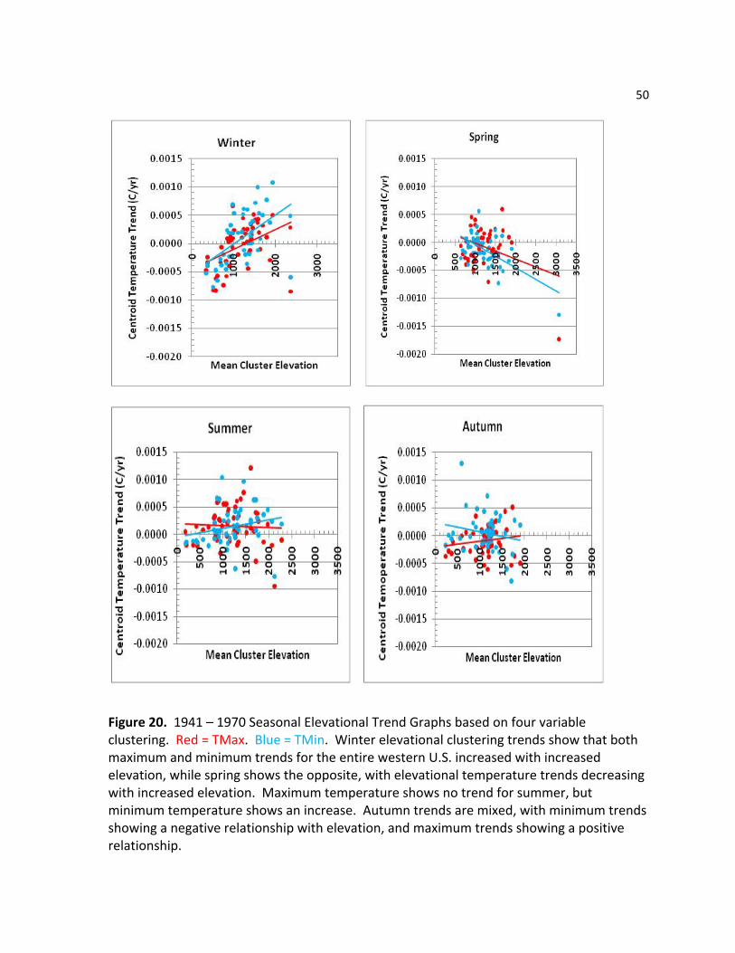
As figure 21 shows, this analysis indicates that a positive relationship exists between
elevation and both winter minimum and maximum temperature trends for the period 1941
-‐1970. This means that temperature trends increased with increasing altitude over the
western U.S., on average. Table 4 indicates that both of these elevational trends are
significant. Spring, on the other hand, experienced significant negative elevational trends

48
over the same time period, but this was due to a strongly negative trend for a cluster
located at about 3000 meters (a statistical outlier). Maximum and minimum trends are
opposite for summer and fall. Summer maximum trends are slightly negative, while
minimum trends are moderately positive. For autumn, however, the opposite is true, with
maximum trends being positive and minimum trends being negative. Neither summer or
fall trends are significant.
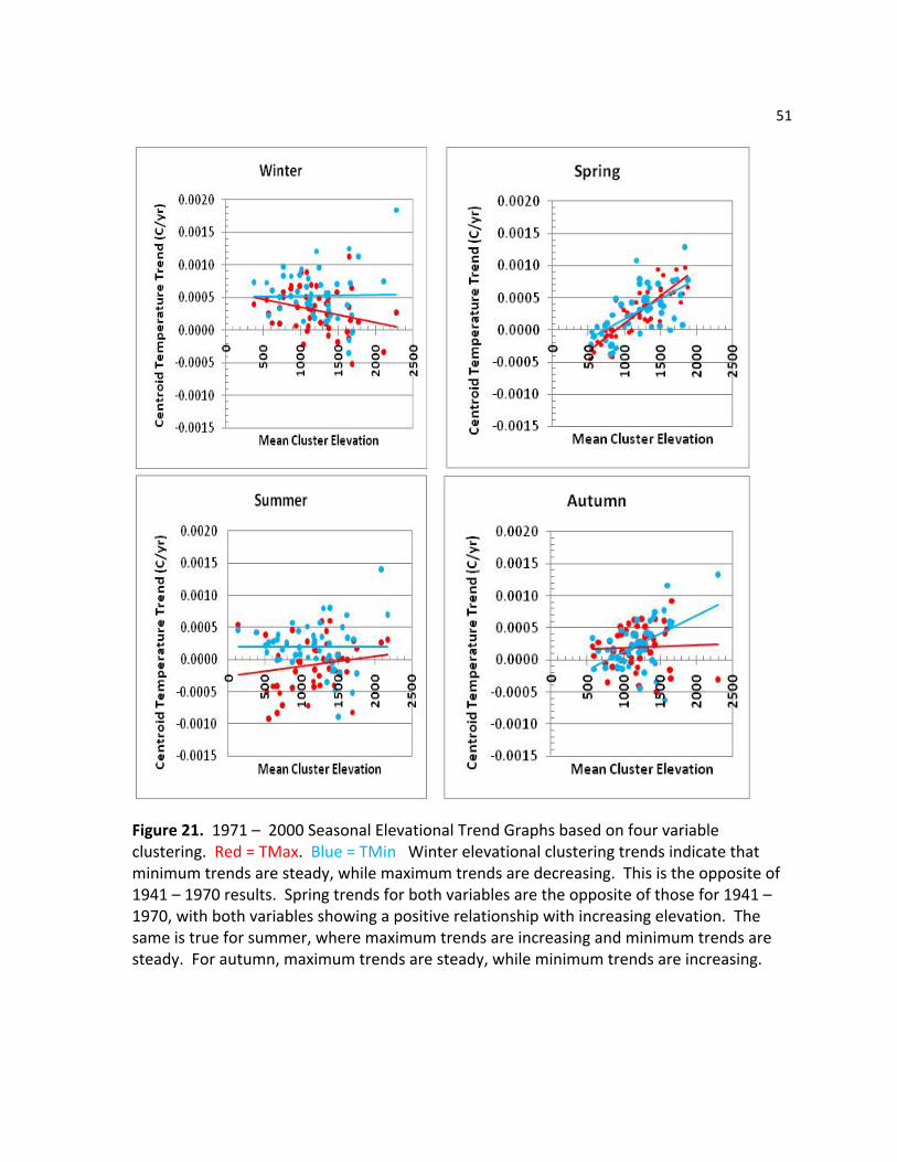
Four variable clustering analysis for the period 1971 – 2000 shows that winter and
spring trends have changed sign for both maximum and minimum temperatures, although
winter’s minimum trend is nearly constant with elevation (figure 21). Maximum winter
trends are now significantly negative, and both spring trends are significantly positive.
Summer maximum trends are now positive, but minimum trends are nearly flat. Autumn
minimum elevational temperature trends are now significantly positive, in contrast to a
negative trend in 1941 – 1970.
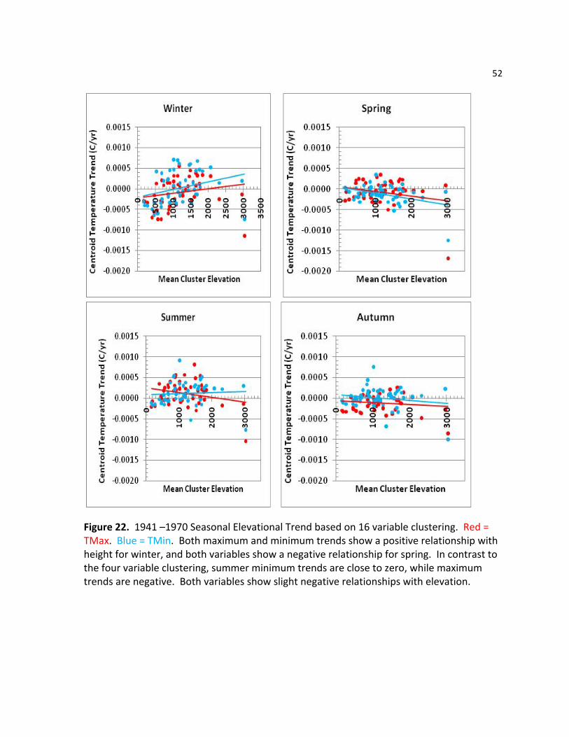
Sixteen variable clustering for 1941 – 1970 produced similar results to that of the
seasonal clustering, where winter trends show a positive relationship with elevation and
spring trends show a negative relationship (figure 22). The main difference for winter and
spring is that the relationships are not as strong, but minimum trends for these seasons
were still significant for this analysis. Both autumn trends are slightly negative, but very
similar. Summer trends were mixed, with slightly positive minimum trends and somewhat
negative maximum trends.
49
Figure 23 shows significantly positive elevational temperature trends for spring for
1971 – 2000. Both winter trends are slightly negative, both in direct contrast to the 1941 –
1970. Summer trends are nearly flat for this period, while both a significantly positive
autumn minimum trend exists alongside a nearly flat maximum trend.
As expected, the four variable clustering produced more significant results than the
sixteen variable (yearly) analysis. This is likely because the yearly analysis operates on
trends averaged over seasonal trends, which are of opposite sign and different magnitudes.
However, the differences between them are important. Seasonal clustering for 1941 – 1970
showed both winter and spring maximum trends to be significant (positive and negative,
respectively), and seasonal clustering for 1971 – 2000 showed winter maximum trends to
be significant, whereas the yearly clustering did not. This indicates that seasonal trends can
be different than or larger than yearly trends. Also, the yearly analysis indicates the same
seasons and time periods as being significant as the seasonal analysis does.
50
Figure 20. 1941 – 1970 Seasonal Elevational Trend Graphs based on four variable clustering. Red = TMax. Blue = TMin. Winter elevational clustering trends show that both maximum and minimum trends for the entire western U.S. increased with increased elevation, while spring shows the opposite, with elevational temperature trends decreasing with increased elevation. Maximum temperature shows no trend for summer, but minimum temperature shows an increase. Autumn trends are mixed, with minimum trends showing a negative relationship with elevation, and maximum trends showing a positive relationship.
51
Figure 21. 1971 – 2000 Seasonal Elevational Trend Graphs based on four variable clustering. Red = TMax. Blue = TMin Winter elevational clustering trends indicate that minimum trends are steady, while maximum trends are decreasing. This is the opposite of 1941 – 1970 results. Spring trends for both variables are the opposite of those for 1941 – 1970, with both variables showing a positive relationship with increasing elevation. The same is true for summer, where maximum trends are increasing and minimum trends are steady. For autumn, maximum trends are steady, while minimum trends are increasing.
52
Figure 22. 1941 –1970 Seasonal Elevational Trend based on 16 variable clustering. Red = TMax. Blue = TMin. Both maximum and minimum trends show a positive relationship with height for winter, and both variables show a negative relationship for spring. In contrast to the four variable clustering, summer minimum trends are close to zero, while maximum trends are negative. Both variables show slight negative relationships with elevation.
53
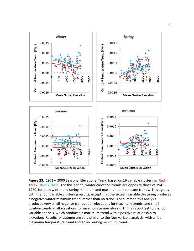
Figure 23. 1971 – 2000 Seasonal Elevational Trend based on 16 variable clustering. Red = TMax. Blue = TMin. For this period, winter elevation trends are opposite those of 1941 – 1970, for both winter and spring minimum and maximum temperature trends. This agrees with the four variable clustering results, except that the sixteen variable clustering produces a negative winter minimum trend, rather than no trend. For summer, this analysis produced very small negative trends at all elevations for maximum trends, and small positive trends at all elevations for minimum temperatures. This is in contrast to the four variable analysis, which produced a maximum trend with a positive relationship to elevation. Results for autumn are very similar to the four variable analysis, with a flat maximum temperature trend and an increasing minimum trend.
54
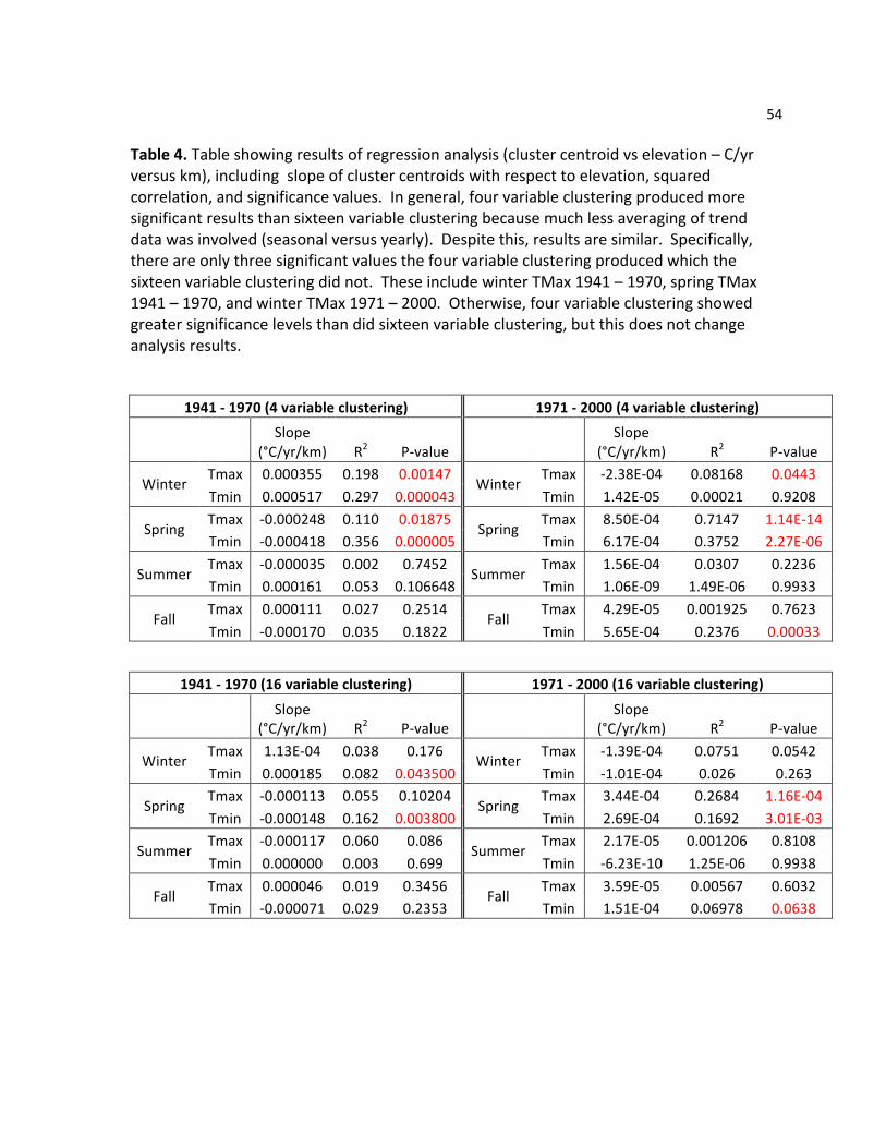
Table 4. Table showing results of regression analysis (cluster centroid vs elevation – C/yr versus km), including slope of cluster centroids with respect to elevation, squared correlation, and significance values. In general, four variable clustering produced more significant results than sixteen variable clustering because much less averaging of trend data was involved (seasonal versus yearly). Despite this, results are similar. Specifically, there are only three significant values the four variable clustering produced which the sixteen variable clustering did not. These include winter TMax 1941 – 1970, spring TMax 1941 – 1970, and winter TMax 1971 – 2000. Otherwise, four variable clustering showed greater significance levels than did sixteen variable clustering, but this does not change analysis results.
1941 -‐ 1970 (4 variable clustering) 1971 -‐ 2000 (4 variable clustering)
Slope
(°C/yr/km) R2 P-‐value Slope
(°C/yr/km) R2 P-‐value
Winter Tmax 0.000355 0.198 0.00147
Winter Tmax -‐2.38E-‐04 0.08168 0.0443
Tmin 0.000517 0.297 0.000043 Tmin 1.42E-‐05 0.00021 0.9208
Spring Tmax -‐0.000248 0.110 0.01875
Spring Tmax 8.50E-‐04 0.7147 1.14E-‐14
Tmin -‐0.000418 0.356 0.000005 Tmin 6.17E-‐04 0.3752 2.27E-‐06
Summer Tmax -‐0.000035 0.002 0.7452
Summer Tmax 1.56E-‐04 0.0307 0.2236
Tmin 0.000161 0.053 0.106648 Tmin 1.06E-‐09 1.49E-‐06 0.9933
Fall Tmax 0.000111 0.027 0.2514
Fall Tmax 4.29E-‐05 0.001925 0.7623
Tmin -‐0.000170 0.035 0.1822 Tmin 5.65E-‐04 0.2376 0.00033
1941 -‐ 1970 (16 variable clustering) 1971 -‐ 2000 (16 variable clustering)
Slope
(°C/yr/km) R2 P-‐value Slope
(°C/yr/km) R2 P-‐value
Winter Tmax 1.13E-‐04 0.038 0.176
Winter Tmax -‐1.39E-‐04 0.0751 0.0542
Tmin 0.000185 0.082 0.043500 Tmin -‐1.01E-‐04 0.026 0.263
Spring Tmax -‐0.000113 0.055 0.10204
Spring Tmax 3.44E-‐04 0.2684 1.16E-‐04
Tmin -‐0.000148 0.162 0.003800 Tmin 2.69E-‐04 0.1692 3.01E-‐03
Summer Tmax -‐0.000117 0.060 0.086
Summer Tmax 2.17E-‐05 0.001206 0.8108
Tmin 0.000000 0.003 0.699 Tmin -‐6.23E-‐10 1.25E-‐06 0.9938
Fall Tmax 0.000046 0.019 0.3456
Fall Tmax 3.59E-‐05 0.00567 0.6032
Tmin -‐0.000071 0.029 0.2353 Tmin 1.51E-‐04 0.06978 0.0638
55
5.2.2 Linear Regression
In addition to k-‐means clustering, linear regression for the mean minimum and
maximum temperatures for each buffered ecoregion against elevation was performed in
order to produce 30 year running means of seasonal elevational temperature trends
(figures 24 -‐ 29). These analyses were done in order to provide more regionally specific
elevational temperature trends, in contrast to the clustering which was done for the entire
western United States. In general, elevational temperature trends are of lower magnitude
than mean temperature trends, but they follow a similar pattern through time. This means
that when mean temperature trends are positive, higher elevations show greater or more
positive temperature trends than do lower elevations. There are some general additional
significant differences for all ranges, however. The most noticeable is that spring’s
elevational trend does not tend to peak around 1965 and then level off, as it does for many
of the mountain ranges mean trends. It continues to rise, in most cases. Seasonal
elevational trends tend to be much more consistent with each other as well, and variability
through time is less than mean trends.
Both minimum and maximum elevational trends in the Cascades closely follow the
pattern of the mean trends. Magnitudes are generally about ½ to 1/3 their value, however.
All seasonal trends for both variables are currently rising. Maximum elevational trends have
experienced a sharp rise since 1975.
Seasonal elevational trends in the Sierra Nevada range also closely follow the
pattern of their mean trends, although their magnitudes are only about ¼ that of the mean
56
trends. Here, maximum trends are more variable than minimum trends. Winter maximum
trends have shown the greatest increase, while summer’s maximum trends have leveled off
since 1960. All seasonal minimum trends have experienced a moderate rise since 1950, and
are very similar in magnitude. No seasonal trend shows a recent, noticeable difference
from the others.
Through 1950, maximum elevational trends for the Northern Rockies are relatively
small, but they do not follow their respect mean temperature trend patterns very closely.
All seasons experience a large decrease to relatively large negative elevational trends (~
0.04°C/yr/km) by 1967, which is starkly different from all other regions. Recently, winter
and fall trends have increased somewhat, but spring and summer trends remain negative.
In contrast, minimum elevational trends are very steady through 1950 as well, but they only
decrease slightly through 1968 and then rise sharply.
The Middle and Southern Rockies, as well as the Wasatch, follow the relatively
steady trend pattern of the Northern Rockies through about 1955. Maximum winter
elevational trends for the Southern Rockies and the Wasatch are the most variable in
comparison to the other seasons, have the largest magnitudes, and are of opposite sign
during the 1920’s and again during the 1950’s. Additionally, these variables do not indicate
a recent increase in elevational trends, as minimum elevational trends for these ranges and
both maximum and minimum elevational trends in the Middle Rockies show. Recent trends
for spring are greatest for the Middle Rockies for both variables, while recent trends for the
Wasatch in fall also show a large increase. The mean seasonal trend patterns and

57
elevational trends for these three ranges do not follow each other as closely as the
Cascades, Sierra Nevada, and Northern Rockies. As Barry (2008) discusses, this may be due
to their greater continentality.
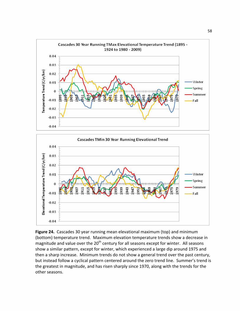
58
Figure 24. Cascades 30 year running mean elevational maximum (top) and minimum (bottom) temperature trend. Maximum elevation temperature trends show a decrease in magnitude and value over the 20th century for all seasons except for winter. All seasons show a similar pattern, except for winter, which experienced a large dip around 1975 and then a sharp increase. Minimum trends do not show a general trend over the past century, but instead follow a cyclical pattern centered around the zero trend line. Summer’s trend is the greatest in magnitude, and has risen sharply since 1970, along with the trends for the other seasons.
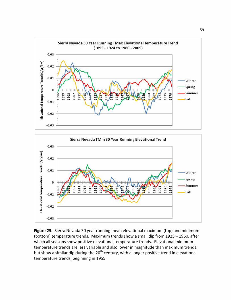
59
Figure 25. Sierra Nevada 30 year running mean elevational maximum (top) and minimum (bottom) temperature trends. Maximum trends show a small dip from 1925 – 1960, after which all seasons show positive elevational temperature trends. Elevational minimum temperature trends are less variable and also lower in magnitude than maximum trends, but show a similar dip during the 20th century, with a longer positive trend in elevational temperature trends, beginning in 1955.
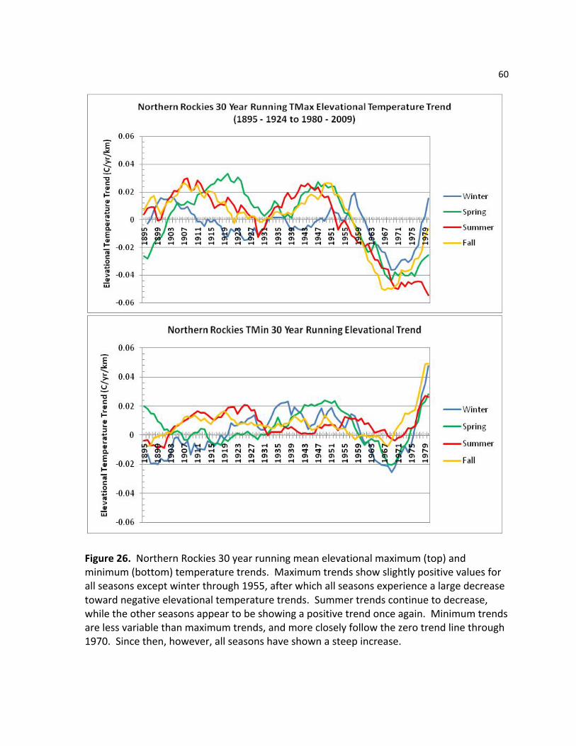
60
Figure 26. Northern Rockies 30 year running mean elevational maximum (top) and minimum (bottom) temperature trends. Maximum trends show slightly positive values for all seasons except winter through 1955, after which all seasons experience a large decrease toward negative elevational temperature trends. Summer trends continue to decrease, while the other seasons appear to be showing a positive trend once again. Minimum trends are less variable than maximum trends, and more closely follow the zero trend line through 1970. Since then, however, all seasons have shown a steep increase.
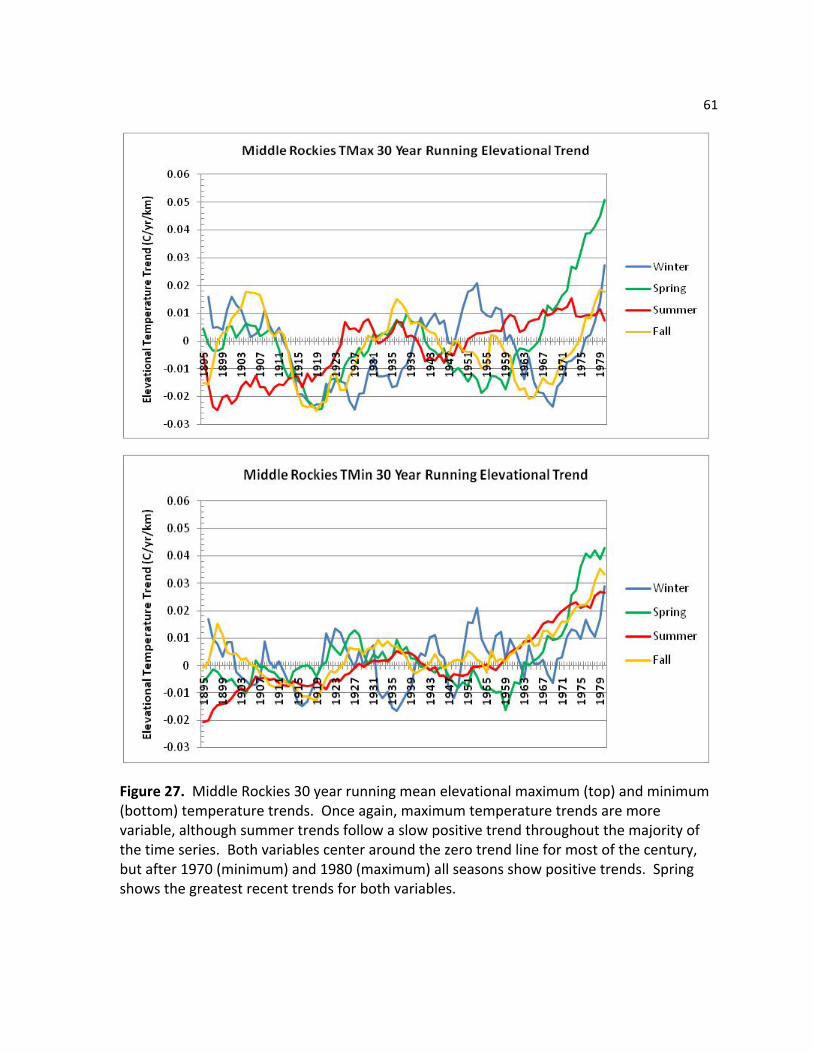
61
Figure 27. Middle Rockies 30 year running mean elevational maximum (top) and minimum (bottom) temperature trends. Once again, maximum temperature trends are more variable, although summer trends follow a slow positive trend throughout the majority of the time series. Both variables center around the zero trend line for most of the century, but after 1970 (minimum) and 1980 (maximum) all seasons show positive trends. Spring shows the greatest recent trends for both variables.
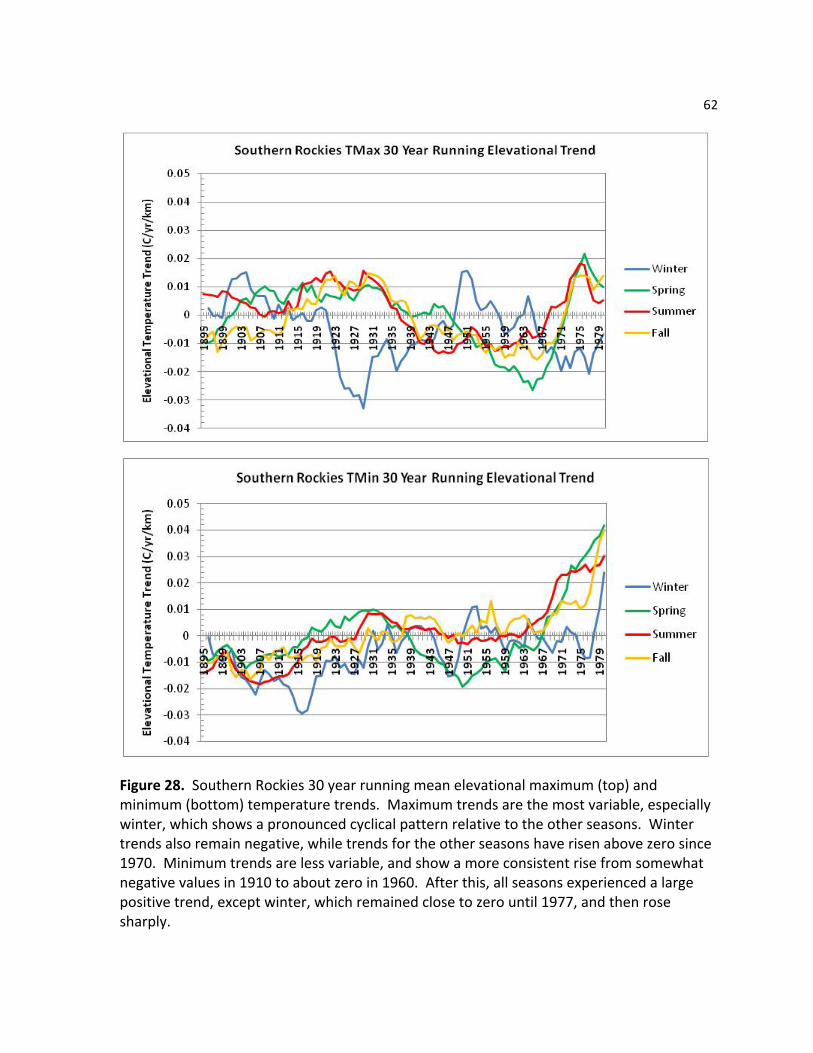
62
Figure 28. Southern Rockies 30 year running mean elevational maximum (top) and minimum (bottom) temperature trends. Maximum trends are the most variable, especially winter, which shows a pronounced cyclical pattern relative to the other seasons. Winter trends also remain negative, while trends for the other seasons have risen above zero since 1970. Minimum trends are less variable, and show a more consistent rise from somewhat negative values in 1910 to about zero in 1960. After this, all seasons experienced a large positive trend, except winter, which remained close to zero until 1977, and then rose sharply.
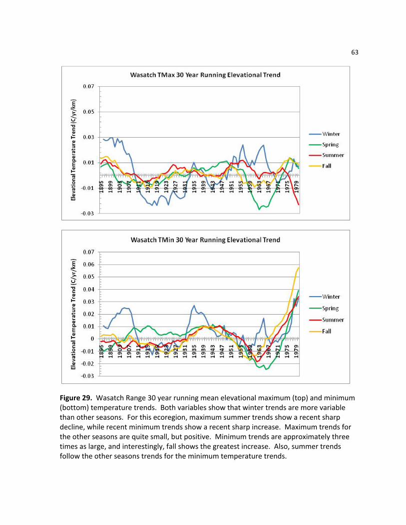
63
Figure 29. Wasatch Range 30 year running mean elevational maximum (top) and minimum (bottom) temperature trends. Both variables show that winter trends are more variable than other seasons. For this ecoregion, maximum summer trends show a recent sharp decline, while recent minimum trends show a recent sharp increase. Maximum trends for the other seasons are quite small, but positive. Minimum trends are approximately three times as large, and interestingly, fall shows the greatest increase. Also, summer trends follow the other seasons trends for the minimum temperature trends.
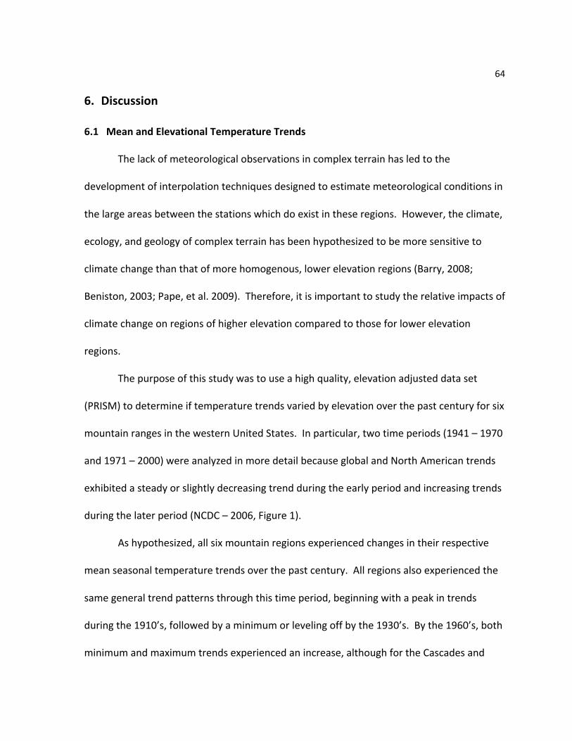
64
6. Discussion
6.1 Mean and Elevational Temperature Trends
The lack of meteorological observations in complex terrain has led to the
development of interpolation techniques designed to estimate meteorological conditions in
the large areas between the stations which do exist in these regions. However, the climate,
ecology, and geology of complex terrain has been hypothesized to be more sensitive to
climate change than that of more homogenous, lower elevation regions (Barry, 2008;
Beniston, 2003; Pape, et al. 2009). Therefore, it is important to study the relative impacts of
climate change on regions of higher elevation compared to those for lower elevation
regions.
The purpose of this study was to use a high quality, elevation adjusted data set
(PRISM) to determine if temperature trends varied by elevation over the past century for six
mountain ranges in the western United States. In particular, two time periods (1941 – 1970
and 1971 – 2000) were analyzed in more detail because global and North American trends
exhibited a steady or slightly decreasing trend during the early period and increasing trends
during the later period (NCDC – 2006, Figure 1).
As hypothesized, all six mountain regions experienced changes in their respective
mean seasonal temperature trends over the past century. All regions also experienced the
same general trend patterns through this time period, beginning with a peak in trends
during the 1910’s, followed by a minimum or leveling off by the 1930’s. By the 1960’s, both
minimum and maximum trends experienced an increase, although for the Cascades and
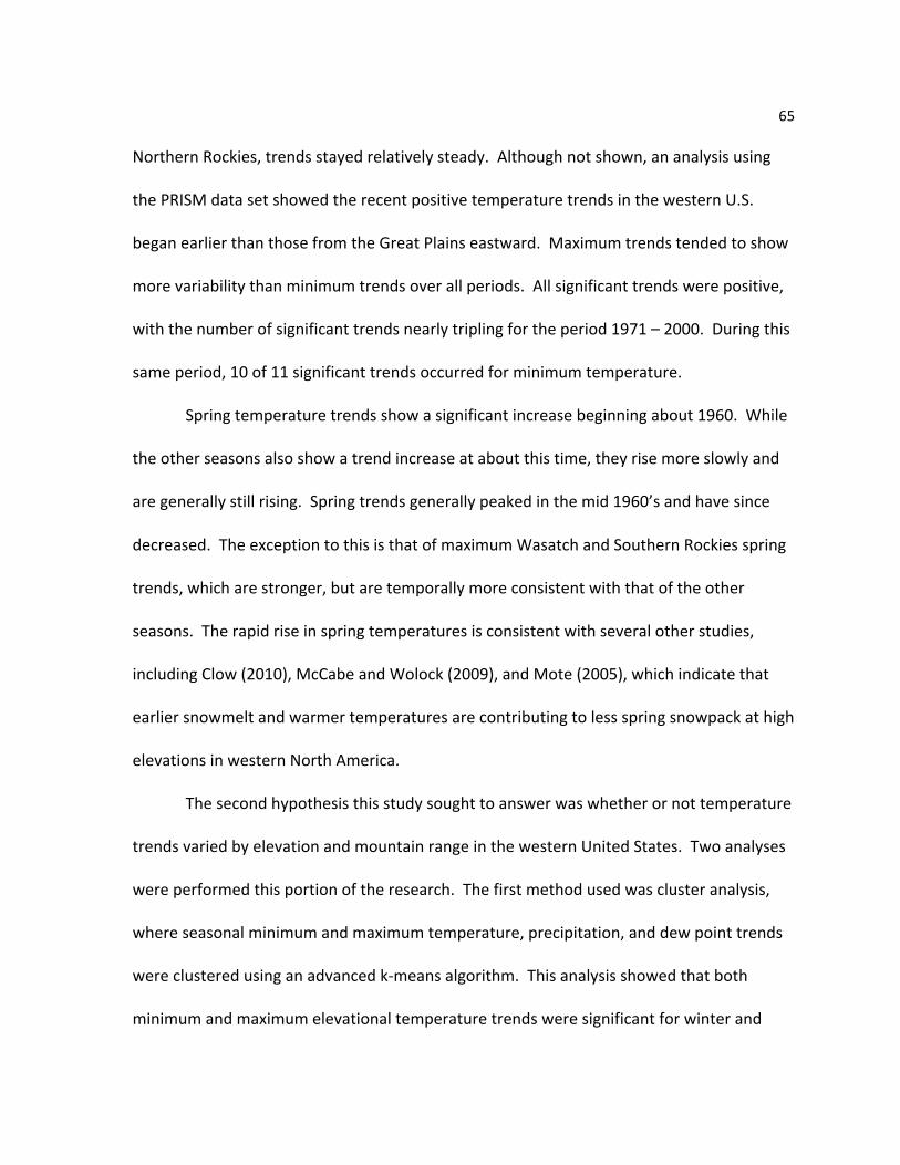
65
Northern Rockies, trends stayed relatively steady. Although not shown, an analysis using
the PRISM data set showed the recent positive temperature trends in the western U.S.
began earlier than those from the Great Plains eastward. Maximum trends tended to show
more variability than minimum trends over all periods. All significant trends were positive,
with the number of significant trends nearly tripling for the period 1971 – 2000. During this
same period, 10 of 11 significant trends occurred for minimum temperature.
Spring temperature trends show a significant increase beginning about 1960. While
the other seasons also show a trend increase at about this time, they rise more slowly and
are generally still rising. Spring trends generally peaked in the mid 1960’s and have since
decreased. The exception to this is that of maximum Wasatch and Southern Rockies spring
trends, which are stronger, but are temporally more consistent with that of the other
seasons. The rapid rise in spring temperatures is consistent with several other studies,
including Clow (2010), McCabe and Wolock (2009), and Mote (2005), which indicate that
earlier snowmelt and warmer temperatures are contributing to less spring snowpack at high
elevations in western North America.
The second hypothesis this study sought to answer was whether or not temperature
trends varied by elevation and mountain range in the western United States. Two analyses
were performed this portion of the research. The first method used was cluster analysis,
where seasonal minimum and maximum temperature, precipitation, and dew point trends
were clustered using an advanced k-‐means algorithm. This analysis showed that both
minimum and maximum elevational temperature trends were significant for winter and
66
spring 1941 – 1970. The trends were positive for winter, but negative for spring. For 1971 –
2000, spring elevation trends were still significant, but now they were positive. Only the
trend for maximum temperature was now significant, but it too had changed sign, to
negative. No summer trends were significant. Minimum fall trends for 1971 – 2000 were
significantly positive. An important note here is that spring 1941 – 1970 trends are likely
significant due to the highly negative trend for the cluster at 3000 meters. Additionally,
yearly averages of these variables, based on seasonal averages, were clustered. This
analysis produced similar, although less significant results. These generally agree with those
found in table 4, showing that yearly results are smaller and are not as significant. Overall,
this analysis indicates that spring temperatures are currently warming faster at higher
elevations than at low elevations.
The second method used to analyze elevational temperature trends was a running
30 year mean for a buffered area around each ecoregion. Here, maximum temperature
trends are more variable, although the magnitude for minimum and maximum trends is
about 1/3 to ½ that of the mean trends. Temperature trends by elevation generally follow a
pattern similar to that of their respective mean ecoregion trends (for example, positive
mean temperature trends tend to occur if temperature trends increase with elevation, and
vice versa). The Northern Rockies maximum trend shows a large decrease around 1960,
while the minimum trend shows a large increase from about 1970. The Cascades and Sierra
Nevada show a smaller average elevational trend magnitude than the other ranges.
Minimum trends experience a larger recent increase than that of maximum trends.
67
Seasonal differences are small. Spring trends are much higher than those of the other
seasons for the Middle Rockies, however. This analysis also indicates that, with the
exception of the maximum trends for the Northern Rockies and possibly Wasatch Range,
higher elevations are warming faster than lower elevations. Virtually no temporal
difference is apparent among seasonal trends for any ecoregion.
Results from this analysis agree with those of Pepin and Lundquist (2008), in the
sense that temperature trends in mountainous regions are not necessarily easily
distinguishable from those elsewhere. However, very generally, both my analyses do
indicate that higher elevations are experiencing greater warming rates (there is also a large
amount of spatial variation, which makes this an inconclusive result for the entire western
U.S.). This is in contrast to the findings of Pepin and Lunquist (2008), who base their results
on GHCN data. A few possible reasons may exist for this discrepancy. One is the different
sources of data used. The other is the difference in time periods analyzed. Pepin and
Lundquist use the period 1948 – 2002 to determine trends, while I essentially break this
period into two separate analyses, each of which produces different results for winter and
spring elevational trends. Pepin and Lundquist do not do a seasonal analysis; nor do they
analyze by ecoregion or mountain range. Additionally, my research seems to indicate the
greatest trends occur further south and for inland mountainous terrain, which is in general
contrast to the results of Pepin and Lundquist. Once again, however, the differences in time
periods may be a significant factor. This may be a valuable area for future research.
68
There is significant uncertainty in these results, both spatially and temporally,
however, due to the lack of stations in these areas. Despite this, overall results from this
study appear to be in line with other research, indicating that spring is warming faster than
other seasons, and recent temperature trends are greater at higher elevations. These
results, including the lack of detailed findings (spatial differences and their causes, for
example), highlight the need for more data collection and continued development and
evaluation of interpolated meteorological data sets. Future sections of this paper discuss
sources of error and suggest future work that may contribute to knowledge about what
drives temperature trends in western North America.
6.2 Potential Role of Large Scale/ Synoptic Regimes
As discussed earlier, mountain meteorology is relatively poorly observed, and as a
result, not well understood, especially at a small scale. Therefore, causes for varying
temperature trends with changing elevation are somewhat difficult to discern. Scully (2010)
indicates that actual temperatures in mountainous areas are controlled much more strongly
by local terrain and other factors, rather than large scale pattern changes, such as ENSO.
This is consistent with observations, which indicate that terrain factors such as aspect and
slope orientation, and local meteorological factors, such as cold air pooling produce the
greatest variations in temperature in these areas.
Table 3 indicates that, in general, mean temperature trends are less significant the
lower in elevation the mountain range is, as well as the more maritime influence it has
(Cascades and Northern Rockies). The combination of high elevation and strong
69
continentality seems to indicate a better likelihood of higher mean temperature trends
(Sierra Nevada, Middle Rockies, and Wasatch Range). Surprisingly, the only significant
mean seasonal trends for the Southern Rockies are for summer minimum temperatures.
This pattern is not explained by greater elevation or continentality. The fact that spring
temperatures show the greatest changes may be explained by earlier snowmelt and
decreasing snowfall (Clow, 2010). Although this particular study was focused on the
Colorado Rockies, similar spring temperature patterns exist in other ranges, perhaps
indicating this is also the case in these areas.
Elevational temperature trends do not appear to follow this same pattern related to
maritime influence and continentality, in general. Table 5 shows these for 1971 -‐ 2000. For
example, nearly all minimum temperature elevational trends are significant for the
Southern Rockies, except for winter and spring, which were the only significant mean
trends. The Cascades (mostly maximum trends) and Northern Rockies (mostly minimum
trends) each show several significant seasonal trends. Rangwala (2008) suggests that
increasing humidity at higher locations may explain why certain high altitude regions
(Tibetan Plateau, in particular) are warming during the winter. Whether or not this is due to
synoptic regime changes is unclear. He also indicates that the snow-‐albedo feedback is a
more important factor for warming during the spring and summer months for the Tibetan
Plateau, which also appears to be valid for the Colorado Rockies.

70
6.3 Sources of Error
As discussed previously, a potentially large source of error is the interpolation
algorithm used by PRISM. However, PRISM data was used because it is specifically adjusted
for elevation, and many studies have concluded that it is the most accurate interpolated
data set (see Reference section). Station data are too sparse at high elevations to
determine elevational temperature trends. As pointed out by Dan Vimont (2010, personal
communication) the linear interpolation used by PRISM may lead to the station trends being
interpolated to different elevations, so that the interpolated trends are artificially similar to
those of the nearby stations used. Although PRISM takes into account inversions, the
analysis of station trends used in PRISM and trends of grid cells based on those stations
would be a good verification step.
The clustering algorithm was designed to minimize potential error in determining
which grid cells were most similar, but this may also be a source of error. There are many
clustering algorithms available, and it may be worthwhile to try other algorithms. Error in
the linear regression analyses can stem from the fact that there are many more stations at
lower elevations than at high elevations. This doesn’t necessarily change the trends,
though. A potential problem is that the number of stations used in the PRISM interpolation
changes with time, potentially influencing the trends. No studies have been done, to the
best of my knowledge, which quantifies the potential impact of this fact. Trend analysis
could be done using only the stations at the beginning of the period, either 1941 or 1971 to
avoid this issue. I am only able to speculate on this issue, however, since the number of
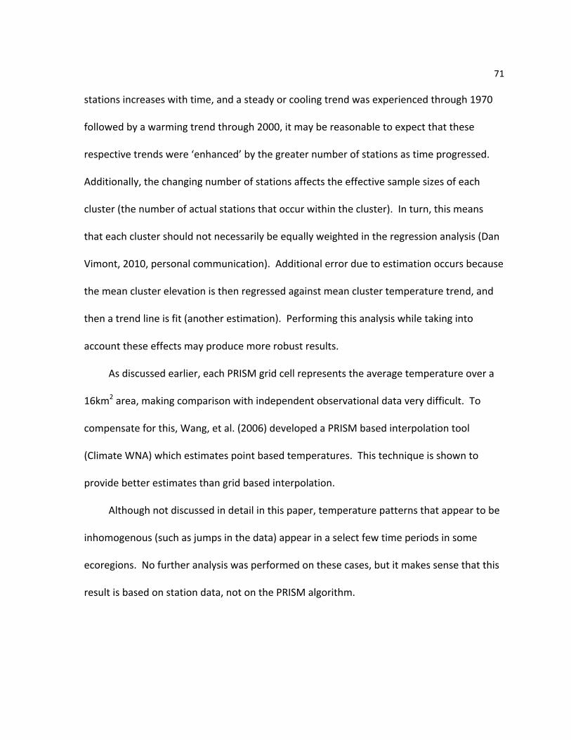
71
stations increases with time, and a steady or cooling trend was experienced through 1970
followed by a warming trend through 2000, it may be reasonable to expect that these
respective trends were ‘enhanced’ by the greater number of stations as time progressed.
Additionally, the changing number of stations affects the effective sample sizes of each
cluster (the number of actual stations that occur within the cluster). In turn, this means
that each cluster should not necessarily be equally weighted in the regression analysis (Dan
Vimont, 2010, personal communication). Additional error due to estimation occurs because
the mean cluster elevation is then regressed against mean cluster temperature trend, and
then a trend line is fit (another estimation). Performing this analysis while taking into
account these effects may produce more robust results.
As discussed earlier, each PRISM grid cell represents the average temperature over a
16km2 area, making comparison with independent observational data very difficult. To
compensate for this, Wang, et al. (2006) developed a PRISM based interpolation tool
(Climate WNA) which estimates point based temperatures. This technique is shown to
provide better estimates than grid based interpolation.
Although not discussed in detail in this paper, temperature patterns that appear to be
inhomogenous (such as jumps in the data) appear in a select few time periods in some
ecoregions. No further analysis was performed on these cases, but it makes sense that this
result is based on station data, not on the PRISM algorithm.
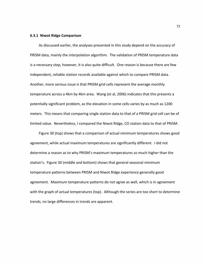
72
6.3.1 Niwot Ridge Comparison
As discussed earlier, the analyses presented in this study depend on the accuracy of
PRISM data, mainly the interpolation algorithm. The validation of PRISM temperature data
is a necessary step, however, it is also quite difficult. One reason is because there are few
independent, reliable station records available against which to compare PRISM data.
Another, more serious issue is that PRISM grid cells represent the average monthly
temperature across a 4km by 4km area. Wang (et al, 2006) indicates that this presents a
potentially significant problem, as the elevation in some cells varies by as much as 1200
meters. This means that comparing single station data to that of a PRISM grid cell can be of
limited value. Nevertheless, I compared the Niwot Ridge, CO station data to that of PRISM.
Figure 30 (top) shows that a comparison of actual minimum temperatures shows good
agreement, while actual maximum temperatures are significantly different. I did not
determine a reason as to why PRISM’s maximum temperatures so much higher than the
station’s. Figure 30 (middle and bottom) shows that general seasonal minimum
temperature patterns between PRISM and Niwot Ridge experience generally good
agreement. Maximum temperature patterns do not agree as well, which is in agreement
with the graph of actual temperatures (top). Although the series are too short to determine
trends, no large differences in trends are apparent.
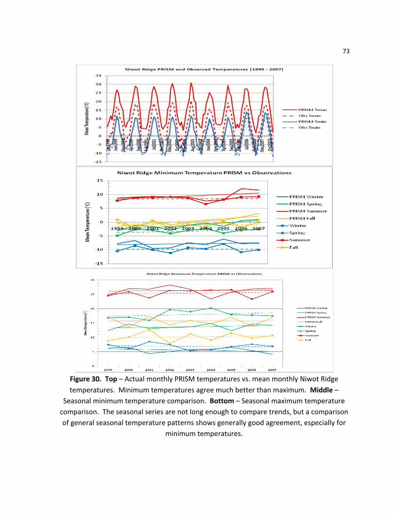
73
Figure 30. Top – Actual monthly PRISM temperatures vs. mean monthly Niwot Ridge temperatures. Minimum temperatures agree much better than maximum. Middle –
Seasonal minimum temperature comparison. Bottom – Seasonal maximum temperature comparison. The seasonal series are not long enough to compare trends, but a comparison of general seasonal temperature patterns shows generally good agreement, especially for
minimum temperatures.

74
6.3.2 Station Grid Cell Comparison
To determine whether or not general PRISM trends are reliable, an analysis
comparing the elevational trends of all station locations within each buffered ecoregion
against the elevational trends generated by the interpolated PRISM data was performed.
Table 5 shows the results of this analysis. With few exceptions, the interpolated PRISM data
are very highly significant due to the large number of grid cells. In virtually every case, the
sign and magnitude of station grid cell elevational trends is comparable to that of the
interpolated data. Their significance tends to be less, however. Interpolated elevational
trends do not show a positive or negative bias with respect to that of station grid cells, nor
do their magnitudes show a positive or negative magnitude bias. Yearly elevational trends
tend to be less significant than seasonal trends, mainly for station locations. In agreement
with previous results, winter and spring trends are the most significant.
One additional aspect of the interpolated PRISM elevational trends is that they
exhibit a cyclical pattern over time, as figures 24 -‐29 show. This provides an argument
against the hypothesis that PRISM methodology produces either a positive or negative bias
in sign or magnitude in trends, since otherwise would expect the same direction in trends
for all regions for both time periods. This is not proof, however.
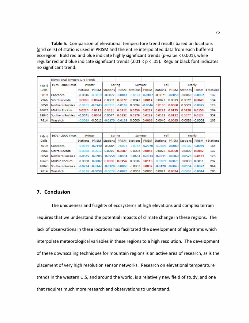
75
Table 5. Comparison of elevational temperature trend results based on locations (grid cells) of stations used in PRISM and the entire interpolated data from each buffered ecoregion. Bold red and blue indicate highly significant trends (p-‐value < 0.001), while regular red and blue indicate significant trends (.001 < p < .05). Regular black font indicates no significant trend.
7. Conclusion
The uniqueness and fragility of ecosystems at high elevations and complex terrain
requires that we understand the potential impacts of climate change in these regions. The
lack of observations in these locations has facilitated the development of algorithms which
interpolate meteorological variables in these regions to a high resolution. The development
of these downscaling techniques for mountain regions is an active area of research, as is the
placement of very high resolution sensor networks. Research on elevational temperature
trends in the western U.S, and around the world, is a relatively new field of study, and one
that requires much more research and observations to understand.
76
Past patterns in mean seasonal temperature trends, as well as seasonal elevational
temperature trends, suggest that the current dramatic rises will not continue. Specific
causes behind this rise are not well understood. However, if anthropogenic climate change
is the driving factor, then these patterns can be expected to continue. If this occurs, then
ecological systems in these locations will be affected.
The uncertainty in these trends is the motivation behind nearly all potential future
work in this research. Data analysis of higher resolution models and high density station
networks will be important. This data is expected to be included in the development of new
interpolated data sets, including TopoMet (Joel Oyler, personal communication, NTSG,
2010), as well as updated PRISM and Daymet data sets (personal communication, Peter
Thornton). Analysis of the PRISM 800 meter data may provide better estimates of
independent station comparison. Additionally, clustering only temperature trends by
individual ecoregions over all 30 year time periods since 1941 may provide better insights
into elevational trends. Part of this may include dividing the ecoregions into smaller parts
(such as splitting the Sierra Nevada into north/south divisions). Region specific snow
cover/temperature trend analyses may provide insight into the effects of the snow-‐ice
albedo feedback process. Empirical orthogonal function analysis and/or principal
component analysis may be able to show similar spatial and temporal patterns among
mountain areas. Finally, comparison of PRISM grid cell values to Climate WNA point
estimates would likely be a valuable study.
77
References Abatzoglou, J.T. (2009). Six million ways to statistically downscale: Decision, merits and limitation. Simulating the Spatial-‐Temporal Patterns of Anthropogenic Climate Change Workshop, Santa Fe, NM, July. Abatzoglou, J.T., Advances in Statistical Meteorological Downscaling: Development and Validation, Tristate EPSCoR Annual Meeting, Incline Village, NV Apr. 2010
Arakawa, Osamu, et al. Intercomparison of the relationship between precipitation and mountain heights among gridded precipitation datasets. Presented at the 23rd Conference on Hydrology, 89th AMS annual meeting, January 11 – 15, 2009, Phoenix, Arizona, USA. Bailey, R. G. 1983. Delineation of ecosystem regions. Environmental Management 7: 365-‐373. Barry, Roger G.(2008). Advances in mountain climate research. Presented at MTNCLIM, Silverton, Colorado, June 9 – 12. -‐-‐-‐-‐-‐-‐ (1992). Mountain climatology and past and potential future climatic changes in mountain regions: a review. Mountain Research and Development. Vol. 12, No. 1, 71 – 86. -‐-‐-‐-‐-‐-‐-‐. Mountain Weather and Climate. Third Edition. New York, New York: Cambridge University Press, 2008.
Beniston, M., and Rebetez, M. (1996). Regional behavior of minimum temperatures in Switzerland for the period 1979 – 1993. Journal of Theoretical and Applied Climatology, Vol. 53, 231– 243. Beniston, M., Diaz,H.F. and Bradley, R.S. (1997). Climatic change at high elevation sites: An overview. Climatic Change, Vol. 36, 233–252. Beniston, Martin. (2003). Climatic change in mountain regions: a review of possible impacts. Climatic Change. Vol. 59, 5 – 31.
Beniston, M. (2006). Mountain weather and climate: A general overview and a focus on climatic change in the Alps. Hydrobiologia, Vol. 562, 3 –16.
78
Blandford, T.R. et al. Interpolating surface air temperature for use in semi-‐distributed snowmelt runoff models. Paper presented at the Western Snow Conference, 2005. Bodine, David, et al. (2009). Variability of surface air temperature over gently sloped terrain. Journal of Applied Meteorology and Climatology, Vol. 48, 1117 – 1141. Bonan, Gordon. Ecological Climatology: Concepts and Applications. Second Edition. New York, New York: Cambridge University Press, 2008. Boni, G., Parodi, A. and Siccardi, F. (2008). A new parsimonious methodology of mapping the spatial variability of annual maximum rainfall in mountainous environments. Journal of Hydrometeorology, Vol. 9, 492 – 506. Borsdorf, Axel (Editor). Newsletter of the Mountain Research Initiative. No. 3, October 2009. Bosch, J.L, et al. (2008). Daily solar irradiation estimation over a mountainous area using artificial neural networks. Renewable Energy, Vol. 33, 1622 – 1628. Bounoua, L. et al. (2002). Effects of land cover conversion on surface climate. Climate Change, Vol. 52, 29 – 64. Bradley, Paul S., et al. (1998). Scaling clustering algorithms to large databases. Proceedings of the 4th International Conference on Knowledge Discovery and Data Mining, R. Agrawal, P. Stolorz and G. Piatesky-‐Shapiro (eds), pp/ 9 – 15. AAAI Press, Menlo Park, CA. Brazel, A. and Outcalt, S.I. (1973). The observation and simulation of diurnal evaporation contrasts in an Alaskan alpine pass. Journal of Applied Meteorology, Vol. 12, 1134 – 1143. Bristow, K.L., and Campbell, G.S. (1984). On the relationship between incoming solar radiation and daily maximum and minimum temperature. Agricultural and Forest Meteorology, Vol. 31, 159-‐166. Campbell, Gaylon S. and Norman, John M. An Introduction to Biophysics. Springer, 1998. Cenedese, Antonio, et al. (1997). Vertical Profiles of Wind, Temperature, and Turbulence. Technical Report. COST Action 710, Working Group #3.
Chen, B., Chao, W.C. and Liu, X. (2003). Enhanced climatic warming in the Tibetan plateau due to doubling CO2: A model study. Climate Dynamics, Vol. 20, 401–413.
79
Chung, Uran, and Yun, Jin I. (2004). Solar irradiance-‐corrected spatial interpolation of hourly temperature in complex terrain. Agricultural and Forest Meteorology, Vol. 126, 129 – 139. -‐-‐-‐-‐-‐-‐-‐-‐-‐, et al. (2006). Minimum temperature mapping over complex terrain by estimating cold air accumulation potential. Agricultural and Forest Meteorology, Vol. 137, 15 – 24. CIRMOUNT Committee. 2006. Mapping New Terrain: Climate Change and America’s West. Report of the Consortium for Integrated Climate Research in Western Mountains (CIRMOUNT), Misc. Pub., PSW-‐MISC-‐77, Albany, CA, Pacific Southwest Research Station, Forest Service, U.S. Department of Agriculture, 29 pp. Clow, David W. (2010). Changes in the timing of snowmelt and streamflow in Colorado: a response to recent warming. Journal of Climate, Vol. 23, 2293 – 2306. Conklin, David R. and Osborne-‐Gowey, Jeremiah D. (2010). In PRISM data, Sierra Nevada warmed only 1°C in the 20th century. Poster presentation at AGU, San Francisco, California, December 13 – 17. Daly, Christopher, et al. (2007). High resolution spatial modeling of daily weather elements for a catchment in the Oregon Cascade Mountains, United States. Journal of Applied Meteorology and Climatology, Vol. 46, 1565 – 1586. -‐-‐-‐-‐-‐-‐-‐-‐-‐. (2008). Physiographically sensitive mapping of climatological temperature and precipitation across the conterminous United States. International Journal of Climatology, DOI: 10.1002. Daly, Christopher and Conklin, David (2008). Hidden climate variability in mountainous terrain. Presented at MTNCLIM, Silverton, Colorado, June 9 – 12. Das, T. et al. (2009). Structure and detectability of trends in hydrological measures over the western United States. Journal of Hydrometeorology, Vol. 10, DOI: 10.1175. Davis, Frank W., et al. (2010). Modeling plant species distributions under future climates: how fine-‐scale do climate models need to be? Presented at AGU, San Francisco, California, December 13 – 17. Diaz, Henry F. and Bradley, Raymond S. (1997). Temperature variations during the last century at high elevation sites. Climatic Change, Vol. 36, 253 – 279.
80
Dobrowski, Solomon Z., et al. (2009). How much influence does landscape-‐scale physiography have on air temperature in a mountain environment? Agricultural and Forest Meteorology, Vol. 149, 1751 – 1758. Durand, Yves, et al. (2009). Reanalysis of 44 years of climate in the French Alps (1958 – 2002): methodology, model validation, climatology, and trends for air temperatures and precipitation. Journal of Applied Meteorology and Climatology, Vol. 48, 429 – 449. Eastman, et al. (2009). Seasonal trend analysis of image time series. International Journal of Remote Sensing. Vol. 30, Nos. 9 – 10, 2721 – 2726. Finardi, Sandro and Morselli, Maria. (1997). Wind Flow Models over Complex Terrain for Dispersion Calculations. Technical Report. COST Action 710, Working Group #4.
Franssen, H. J., and Scherrer, S.C. (2007). Freezing of lakes on the Swiss plateau in the period 1901 – 2006. International Journal of Climatology,Vol. 28, 421 – 433. Giorgi, Filippo, et al. (1997). Elevation dependency of the surface climate change signal: A model study. Journal of Climate, Vol. 10, 288 – 296.
Glassy, J.M., and Running, S.W. (1994). Validating diurnal climatology of the MT-‐CLIM model across a climatic gradient in Oregon. Ecological Applications, Vol. 4, No. 2, 248-‐257. Goovaerts, P. (2000). Geostatistical approaches for incorporating elevation into the spatial interpolation of rainfall. Journal of Hydrology, Vol. 228, 113 – 129. Grosjean, Martin. (2001). Climate Change at high elevation sites: emerging impacts HIGHEST II. Report on a joint NOAA/NSF/SwissNF/Swiss Academies of Sciences/NCRR – Climate Workshop, June 25 – 28. Davos, Switzerland. Mountain Research and Development, Vol. 21, No. 4. Guan, Huade and Wilson, John L. (2005). Geostatistical mapping of mountain precipitation incorporating autosearched effects of terrain and climatic characteristics. Journal of Hydrometeorology, Vol. 6, 1018 – 1030. Hall, Alex., et al. (2003). Mountain influence on climate. October 17. MISR. Hartigan, J. A. 1975. Clustering Algorithms. New York: John Wiley& >>Sons. ISBN 0-‐471-‐35645-‐X.
81
Hasenauer, Hubert, et al. (2003). Validating daily climate interpolations over complex terrain in Austria. Agricultural and Forest Meteorology, Vol. 119, 87 – 107. Hicke, Jeffrey A. and Meddens, Arjan. (2008). Climate influences on plant growth: using satellite observations to predict future patterns. Presented at MTNCLIM, Silverton, Colorado, June 9 – 12. Hihmans, Robert J., et al. (2005). Very high resolution interpolated climate surfaces for global land areas. International Journal of Climatology, Vol. 25, 1965 – 1978. Im, E.S. et al. (2010). Local effects of climate change over the Alpine region: A study with a high resolution climate model with a surrogate climate change scenario. Geophysical Research Letters, Vol. 37, L05704. Isaak, Daniel J., et al. (2010). Massive air and stream temperature sensor networks for studying microclimatic variation in mountain landscapes. Poster presentation at AGU, San Francisco, California, December 13 – 17. Jarvis, Claire H. and Stuart, Neil. (2000). A comparison among strategies for interpolating maximum and minimum daily air temperatures, Part I: The selection of “guiding” topographic and land cover variables. Journal of Applied Meteorology, Vol. 40, 1060 – 1074. Jenkner, J. et al. (2010). Detection and climatology of fronts in a high-‐resolution model reanalysis over the Alps. Meteorological Applications, Vol. 17, 1 -‐ 18. Jones, P. D., and Moberg, A. (2003). Hemispheric and large scale surface air temperature variations: An extensive revision and an update to 2001. Journal of Climatology, Vol. 16, 206– 223.
de Jong, et al. Climate and Hydrology of Mountain Areas. John Wiley & Sons, 2005. Kang, S., Lee, D. and Kimball, J.S. (2004). The effects of spatial aggregation of complex topography on hydroecological process simulations within a rugged forest landscape: development and application of a satellite-‐based topoclimatic model. Canadian Journal of Forest Research, Vol. 34, 519 – 530. Kettle, Helen and Thompson, Roy. (2004). Statistical downscaling in European mountains: verification of reconstructed air temperature. Climate Research, Vol. 26, 97 – 112.
Kimball, J.S., et al., (1997). An improved method for estimating surface humidity from daily minimum temperature. Agricultural and Forest Meteorology, Vol. 85, 87-‐98.
82
Lanzante, J. R., et al. (2003). Temporal homogenization of monthly radiosonde temperature data: Part II: Trends, sensitivities and MSU comparison. Journal of Climatology, Vol. 16, 241–262.
Laternser, M., and Schneebeli, M. (2003). Long term snow climate trends of the Swiss Alps (1931– 1999). International Journal of Climatology, Vol. 23, 733– 750. Lazarus, Steven M. et al. (2002). Near real-‐time application of a mesoscale analysis system to complex terrain. Weather and Forecasting, Vol. 17, 971 – 1000. Lenoir, J. et al. (2008). A significant upward shift in plant species optimum elevation during the 20th century. Science, Vol. 320, 1768 – 1771. Liechti, Sandra and Greenwood, Gregory. (Editors). Newsletter of the Mountain Research Initiative. No. 5, December 2010.
Liu, X. D., and Chen, B.D. (2000). Climatic warming in the Tibetan plateau during recent decades. International Journal of Climatology, Vol. 20, 1729–1742.
Liu, X., Yin, Z.-‐Y., Shao, X., and Qin, N. (2006). Temporal trends and variability of
daily maximum and minimum, extreme temperature events, and growing season length over the eastern and central Tibetan Plateau during 1961 – 2003. Journal of Geophysical Research, Vol. 111, D19109. Lookingbill, Todd R. and Urban, Dean L. (2003). Spatial estimation of air temperature differences for landscape-‐scale studies in montane environments. Agricultural and Forest Meteorology, Vol. 114, 141 – 151. Lundquist, Jessica D. and Cayan, Daniel R. (2007). Surface temperature patterns in complex terrain: daily variations and long term change in the central Sierra Nevada, California. Journal of Geophysical Research, Vol. 112, D11124. Lundquist, Jessica, et al. (2008). Mapping temperature across complex terrain. Presented at MTNCLIM, Silverton, Colorado, June 9 – 12. -‐-‐-‐-‐-‐-‐-‐-‐-‐-‐, et al. (2008). Automated algorithm for mapping regions of cold air pooling in complex terrain. Journal of Geophysical Research, Vol. 113, D22107. Maayar, Mustapha and Chen, Jing M. (2006). Spatial scaling of evapotranspiration as affected by heterogeneities in vegetation, topography, and soil texture. Remote Sensing of Environment, Vol. 102, 33 – 51.
83
McCabe, Gregory J. and Wolock, David M. (2009). Recent declines in western U.S. snowpack in the context of 20th century climate variability. Earth Interactions, Vol. 13, No. 13 – 012.
McCutchan, M. H. (1983). Comparing temperature and humidity on a mountain slope and in the free air nearby. Monthly Weather Review, Vol. 111, 836– 845.
Mears, C. A., et al. (2003). A reanalysis of the MSU channel 2 tropospheric temperature record. Journal of Climatology, Vol. 16, 3650–3664.
Meier, M. F., et al. (2003). The health of glaciers: Recent changes in glacier regime.
Climatic Change, Vol. 59, 123– 135.
Mote, P. W., et al. (2005). Declining mountain snowpack in western North America. Bulletin of the American Meteorological Society, Vol. 86, 39– 49.
Millar, C.I., Westfall, R.D., and Delany, D.L. (2010). Thermal regimes of periglacial
talus landforms: complex micro-‐climatic processes in the Sierra Nevada, California. Presented at MTNCLIM, Blue River, Oregon, June 7 – 10.
Miller, Jim and Rangwala, I. (2010). Enhanced temperature increases in high altitude
regions. Presented at MTNCLIM, Blue River, Oregon, June 7 – 10. Neff, W. D., and King, C. W. (1989). The accumulation and pooling of drainage flows
in a large basin. Journal of Applied Meteorology, Vol. 28, 518– 529. Nogues-‐Bravo, D. et al. (2007). Exposure of global mountain systems to climate warming during the 21st century. Global Environmental Change, Vol. 17, 420 – 428. Oki, T. and Musiake, K. (1991). Spatial rainfall distribution at a storm event in mountainous regions, estimated by orography and wind direction. Water Resources Research, Vol. 27, No. 3, 359 – 369. Pape, Roland et al.(2009). Modelling near-‐surface temperature conditions in high mountain environments: an appraisal. Climate Research, Vol. 39, 99 – 109. Pages, Meritxell and Miro, Josep Ramon. (2010). Determining temperature lapse rates over mountain slopes using vertically weighted regression: a case study from the Pyrenees. Meteorological Applications, Vol. 17, 53 – 63. Pauchard, Anibal, et al. (2009). Ain’t no mountain high enough: plant invasions reaching new elevations. Frontiers in Ecology and the Environment, Vol. 7, No. 9, 479 – 486.
84
Pepin, N. C., and Losleben, M.L. (2002). Climate change in the Colorado Rocky Mountains: Free air versus surface temperature trends. International Journal of Climatology, Vol. 22, 311 – 329. Pepin, Nick and Lundquist, Jessica. Temperature trends in North American mountains: a global context. Poster. Presented at CIRMOUNT, Silverton, CO, June 9 – 12, 2008. Pepin, Nicholas, et al. The influence of cold air drainage on spatial patterns of surface temperature trends in the western U.S. Poster.
Pepin, N. C., and Norris, J. (2005). An examination of the differences between surface and free air temperature trend at high elevation sites: Relationships with cloud cover, snow cover and wind. Journal of Geophysical Research, Vol. 110, D24112. Pepin, N.C. and Seidel,Dian J. (2005). A global comparison of surface and free air temperatures at high elevations. Journal of Geophysical Research, Vol. 110, D03104. Pepin, Nicholas and Kidd, David. (2006). Spatial temperature variation in the Eastern Pyrenees. Weather, Vol. 6, No. 11, 300 – 310. Pepin, N.C. and Lundquist, J.D. (2008). Temperature trends at high elevations: Patterns across the globe. Geophysical Research Letters, Vol. 35, L14701. Peterson, Dave, et al. (2005). Effects of climatic variability and change on Forest Ecosystems – empirical evidence from the Western Mountain Initiative. Presented at MTNCLIM, Chico Hot Springs, Montana, March 1-‐ 4. Pinard, J.-‐P. et al. (2008). Mesoscale wind climate modeling in steep mountains. Atmosphere-‐Ocean, Vol. 47, No. 1, 63 – 78. Prudhomme, Christel and Reed, Duncan W. (1999). Mapping extreme rainfall in a mountainous region using geostatistical techniques: A case study in Scotland. International Journal of Climatology, Vol. 19, 1337 – 1356. Rangwala, I., et al. (2008). Influence of increasing surface humidity on winter warming at high altitudes through the 21st century. Presented at AGU, San Francisco, California, December 15 – 19. Ranhao, Sun, et al. (2008). A multivariate regression model for predicting precipitation in the Daqing Mountains. Mountain Research and Development, Vol. 28, No. 3, 318 – 325.
85
Redmond, Kelly. T. Climate in three dimensions: integrated mountain climate observations. Presented at the CCSP Workshop (Climate Science in Support of Decision Making), Arlington, VA, November 14 – 16, 2005. -‐-‐-‐-‐-‐-‐-‐-‐-‐-‐. (2008). The MTNCLIM Year: Western Climate 2007 – 2008 in Perspective. CIRMOUNT: Anticipating Challenges to Western Mountain Ecosystems and Resources. Silverton, Colorado, June 9 – 12. Rich, Paul M. and Fu, Pinde. (2000). Topoclimate Habitat Models. 4th International Conference on Integrating GIS and Environmental Modeling (GIS/EM4): Problems, Prospects, and Research Needs. Banff, Alberta, Canada. September 2 – 8, 2000. Richards, Katrina. Topoclimates and topoclimate mapping: what do the scientific abstracts tell us about research perspectives? Presented at SIRC – The 14th Annual Colloquium of the Spatial Information Research Centre, University of Otago, Dunedin, New Zealand, December 3 – 5, 2002. Rolland, Christian. (2002). Spatial and seasonal variations of air temperature lapse rates in alpine regions. Journal of Climate, Vol. 16, 1032 – 1046.
Running, S.W., et al. (1987). Extrapolation of synoptic meteorological data in mountainous terrain and its use for simulating forest evaporation and photosynthesis. Canadian Journal of Forest Research, Vol 17, 472-‐483.
Scheifinger, Helfried and Kromp-‐Kolb, Helga. (2000). Modeling global radiation in complex terrain: comparing two statistical approaches. Agricultural and Forest Meteorology, Vol. 100, 127 – 136. Scully, Rebecca A. (2010). Intercomparison of PRISM and Daymet temperature interpolation from 1980 to 2003. Master’s Thesis, Utah State University. Major professor – Dr. Michael White.
Seidel, D. J., and Free, M. (2003). Comparison of lower-‐tropospheric temperature climatologies and trends at low and high elevation radiosonde sites. Climatic Change, Vol. 59, 53– 74.
Seidel, D. J., et al. (2004). Uncertainty in signals of large-‐scale climate variations in radiosonde and satellite upper-‐air temperature datasets. Journal of Climatology, Vol. 17, 2225– 2240. Simeral, David B. and Abatzaglou, John T. (2008). Verification of gridded climate data in mountainous terrain. Poster presentation at CIRMOUNT, Silverton, Colorado, June 9 – 12.
86
Shea, Joseph M. et al. Estimating meteorological variables within glacier boundary layers, Southern Coast Mountains, British Columbia, Canada. Paper presented at the 17th Conference on Applied Climatology, American Meteorological Society, August 11 – 15, 2008, Whistler, BC, Canada.
Sheridan, Peter, et al. (2010). A simple height-‐based correction for temperature downscaling in complex terrain. Meteorological Applications, Vol. 10, DOI: 10.1002.
Shinker, Jacqueline J. (2010). Visualizing spatial heterogeneity of western U.S. climate variability. Earth Interactions. Vol. 14, Paper 14-‐010.
Simpson, James J., et al. (2002). Long-‐term climate patterns in Alaskan surface
temperature and precipitation and their biological consequences. IEEE Transactions on Geoscience and Remote Sensing, Vol. 40, No. 5, 1164 – 1184.
Stahl, K. et al. (2006). Comparison of approaches for spatial interpolation of daily air temperature in a large region with complex topography and highly variable station density. Agricultural and Forest Meteorology, Vol. 139, 224 – 236. Stull, Roland B. An Introduction to Boundary Layer Meteorology. Springer, 2009. Theurillat, J.P. and A. Guisan, 2001: Potential impact of climate change on vegetation in the European Alps: a review. Climatic Change, 50, 77-‐109.
Thornton, P.E., et al., (1997). Generating surfaces of daily meteorological variables over large regions of complex terrain. Journal of Hydrology, Vol. 190, 214-‐251.
Thornton, P.E., and Running, S.W. (1999). An improved algorithm for estimating incident daily solar radiation from measurements of temperature, humidity, and precipitation. Agricultural and Forest Meteorology, Vol. 93, 211-‐228.
Vuille, M., and Bradley, R.S. (2000). Mean annual temperature trends and their vertical structure in the tropical Andes. Geophysical Research Letters, Vol. 27, 3885– 3888.
Vuille, M., et al. (2003). 20th century climate change in the tropical Andes: Observations and model results. Climatic Change, Vol. 59, 75– 99. Wang, Kaicun, et al. (2005). Estimating solar radiation over complex terrain using moderate resolution satellite sensor data. International Journal of Remote Sensing, Vol. 26, No. 1, 47 -‐58.
Wang, Tongli, et al. (2006). Development of scale-‐free climate data for western Canada for use in resource management. International Journal of Climatology, Vol. 26, 383 – 397.

87
Weiss, Stuart B. (2010). From butterflies to bristlecones: microclimatic and topoclimatic range adjustments as a foundation for conservation in a changing macroclimate. Presented at MTNCLIM, Blue River, Oregon, June 7 – 10. Wilby, Rob. Statistical downscaling: Status and open issues. Loughborough University, UK.
Whiteman, C. D., et al. (2001). Cold pools in the Columbia Basin. Weather Forecasting, Vol. 16, 432– 447.
-‐-‐-‐-‐-‐. Mountain meteorology: fundamentals and applications. New York, New York.
Oxford University Press, 2000. Woodwell, G.M., 2004: Mountains: top down. Ambio Special Report, 13, 35-‐38. XU Li-‐ren, et al. Dynamic simulation of mountain valley circulation over complex terrain. Presented at the 2008 Asia Simulation Conference – 7th International Conference on Systematic Simulation and Scientific Computing. Yim, Steve H.L., et al. (2007). Developing a high resolution wind map for complex terrain with a coupled MM5/CALMET system. Journal of Geophysical Research, Vol. 112, D05106. Zald, Harold S.J. (2010). Multiscale climatic, topographic, and biotic controls of tree invasion in a sub-‐alpine parkland landscape, Jefferson Park, Oregon Cascades, USA. Presented at MTNCLIM, Blue River, Oregon, June 6 -‐9. Zhang, Xuesong and Srinivasan, Raghavan. (2009). GIS-‐based spatial precipitation estimation: a comparison of geostatistical approaches. Journal of the American Water Resources Association, Vol. 45, No. 4, 894 – 906.
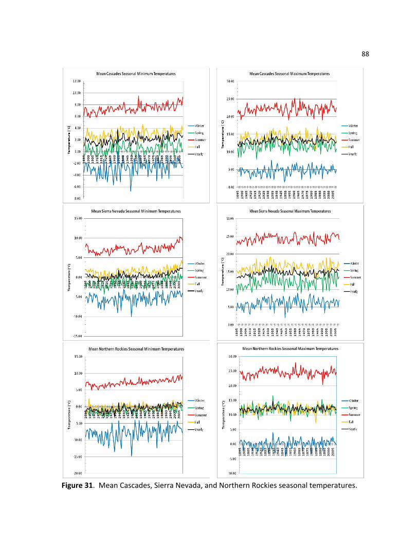
88
Figure 31. Mean Cascades, Sierra Nevada, and Northern Rockies seasonal temperatures.
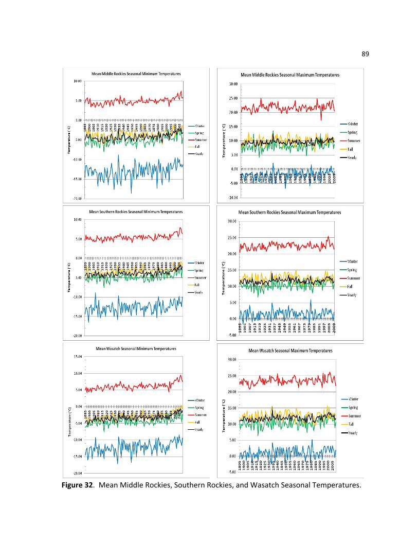
89
Figure 32. Mean Middle Rockies, Southern Rockies, and Wasatch Seasonal Temperatures.
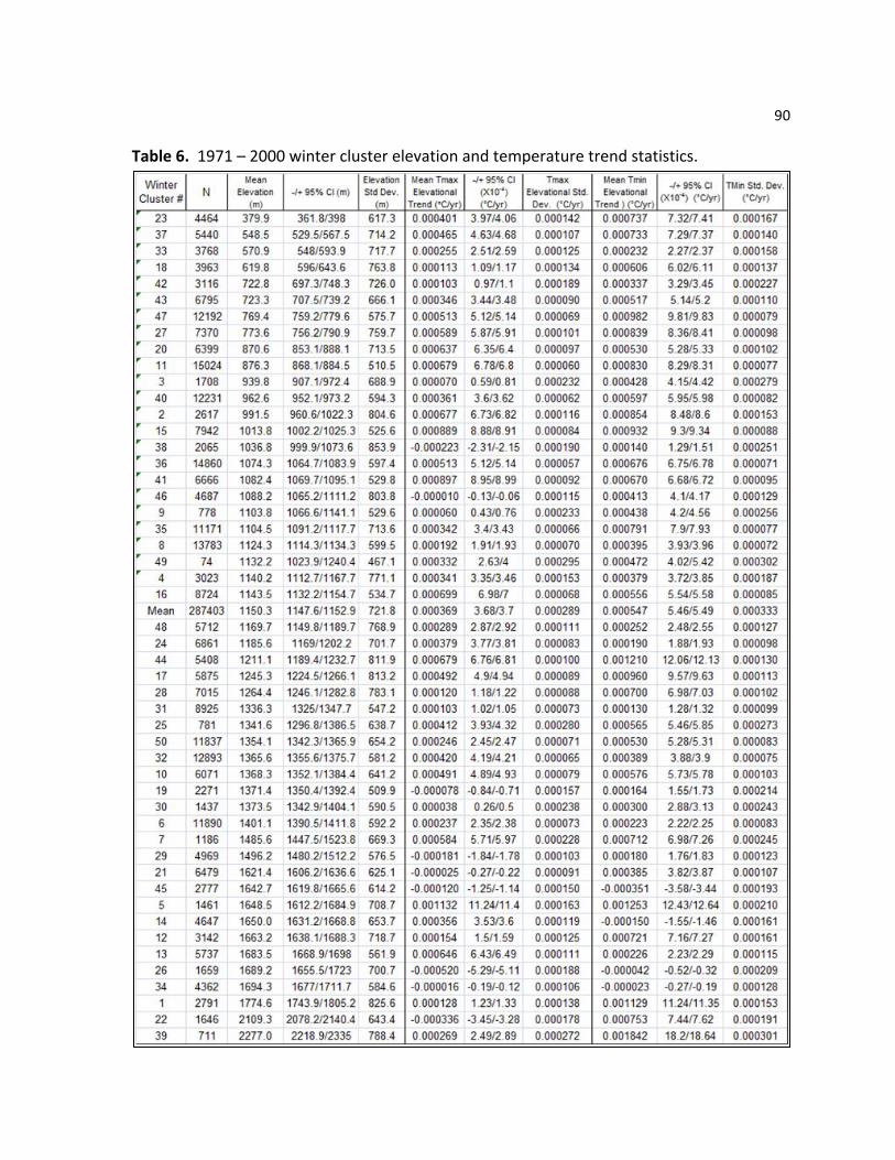
90
Table 6. 1971 – 2000 winter cluster elevation and temperature trend statistics.
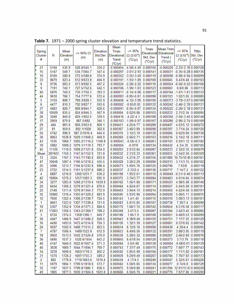
91
Table 7. 1971 – 2000 spring cluster elevation and temperature trend statistics.
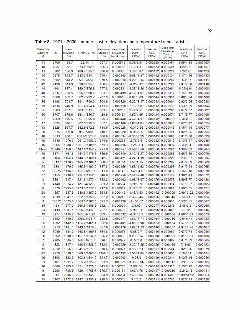
92
Table 8. 1971 – 2000 summer cluster elevation and temperature trend statistics.
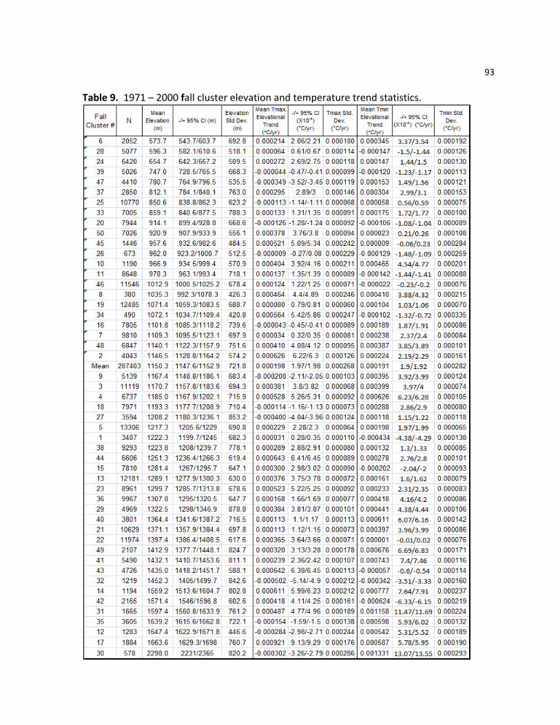
93
Table 9. 1971 – 2000 fall cluster elevation and temperature trend statistics.
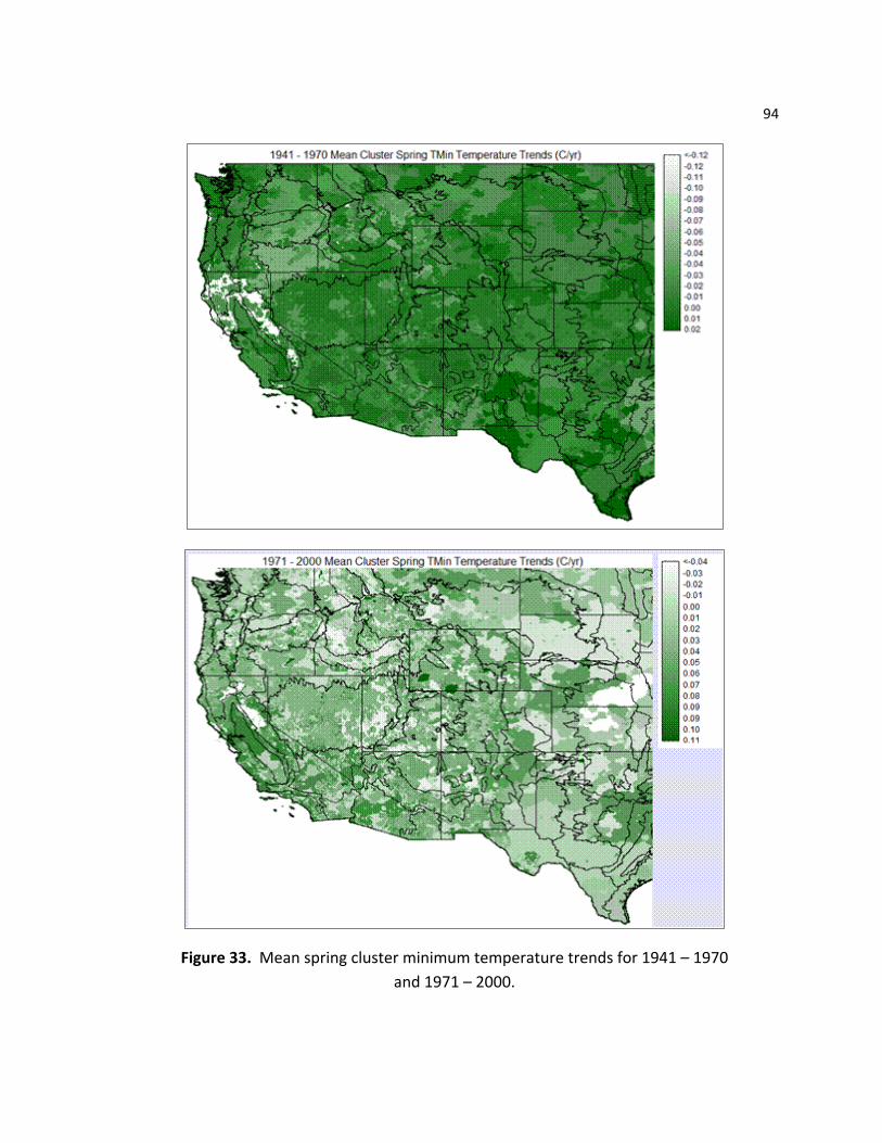
94
Figure 33. Mean spring cluster minimum temperature trends for 1941 – 1970 and 1971 – 2000.
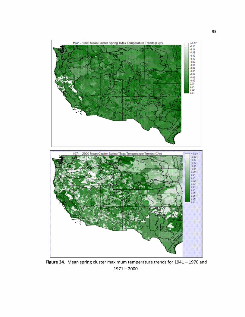
95
Figure 34. Mean spring cluster maximum temperature trends for 1941 – 1970 and
1971 – 2000.