Embed Size (px)
Citation preview

Behavioural Financial DecisionMaking Under Uncertainty
�Hongyu Jiang
St Edmund Hall
University of Oxford
A dissertation submitted for the degree of
MSc in Mathematical and Computational Finance
20 June, 2008


Abstract
Ever since von Neumann and Morgenstern published the axiomisation of
Expected Utility Theory, there have been a considerable amount of ob-
servations appeared in the literature violating the expected utility theory.
To make decisions under uncertainty, people generally separate possible
outcomes into gains and losses. They are risk averse for gains but risk
seeking for losses with very large probabilities; risk averse for losses but
risk seeking for gains with very small probabilities. To accommodate
these characteristics, Prospect Theory and its improvement Cumulative
Prospect Theory were developed in order to formulate people’s behaviours
under uncertainty in a descriptive and normative way. As such, values are
assigned to gains and losses and probabilities are replaced by probability
weighting functions. The CPT models built in this project are based on
the power value function and the compound invariant form of probability
weighting function. The models are calibrated with the data from Hong
Kong Mark Six lottery market. The parameters in the models are esti-
mated, hence to examine properties of the models and give an insights into
how they fit the real life situation. In the first approach, the parameter
in the value function is fixed, but the plots of the estimated probability
weighting function do not give sensible explanations of lottery player’s
behaviours. In the second approach, the parameters in value function and
weighting function are both estimated from the data to give an optimal
fitting of the model.


Contents
1 Introduction 1
1.1 Utility and Expected Utility Theory . . . . . . . . . . . . . . . . . . . 1
1.2 Violations of Expected Utility Theory . . . . . . . . . . . . . . . . . . 4
1.3 Prospect Theory . . . . . . . . . . . . . . . . . . . . . . . . . . . . . 6
1.4 Cumulative Prospect Theory . . . . . . . . . . . . . . . . . . . . . . . 7
1.5 Aim of the Project . . . . . . . . . . . . . . . . . . . . . . . . . . . . 7
1.6 Organisation of the Dissertation . . . . . . . . . . . . . . . . . . . . . 8
2 Theoretical Framework 9
2.1 Cumulative Presentation of Uncertainty . . . . . . . . . . . . . . . . 9
2.2 Axiomisation of CPT . . . . . . . . . . . . . . . . . . . . . . . . . . . 12
2.3 Values and Weights . . . . . . . . . . . . . . . . . . . . . . . . . . . . 13
2.4 Compound Invariant Weighting Functions . . . . . . . . . . . . . . . 15
3 Numerical Experiment 21
3.1 Mark Six . . . . . . . . . . . . . . . . . . . . . . . . . . . . . . . . . . 21
3.2 Data . . . . . . . . . . . . . . . . . . . . . . . . . . . . . . . . . . . . 22
3.3 Single-Factor Model . . . . . . . . . . . . . . . . . . . . . . . . . . . . 23
3.3.1 Algorithm . . . . . . . . . . . . . . . . . . . . . . . . . . . . . 25
3.3.2 Summary of Results . . . . . . . . . . . . . . . . . . . . . . . 26
3.4 Two-Factor Model . . . . . . . . . . . . . . . . . . . . . . . . . . . . 29
3.4.1 Least Squares Estimation . . . . . . . . . . . . . . . . . . . . 30
3.4.2 Summary of Results . . . . . . . . . . . . . . . . . . . . . . . 32
4 Summary and Outlook 37
4.1 Summary . . . . . . . . . . . . . . . . . . . . . . . . . . . . . . . . . 37
4.2 Outlook . . . . . . . . . . . . . . . . . . . . . . . . . . . . . . . . . . 38
Bibliography 38
i

ii

List of Figures
2.1 Plot of the value function v(x) as in equation (2.6) with α = β = 0.88
and λ = 2.25. . . . . . . . . . . . . . . . . . . . . . . . . . . . . . . . 14
2.2 Plot of the probability weighting functions w+(p) = pγ
(pγ+(1−p)γ)1/γand
w−(p) = pδ
(pδ+(1−p)δ)1/δ with γ = 0.61 and δ = 0.69. . . . . . . . . . . . 15
2.3 Plot of the function w(p) = exp{−β(−ln p)α} with fixed value of β =
0.5, α is 0.001, 0.25, 0.5, 0.75, 1, 1.5, 2, 5, 100. . . . . . . . . . . . . . . 18
2.4 Plot of the function w(p) = exp{−β(−ln p)α} with fixed value of β = 1,
α is 0.001, 0.25, 0.5, 0.75, 1, 1.5, 2, 5, 100. . . . . . . . . . . . . . . . . . 19
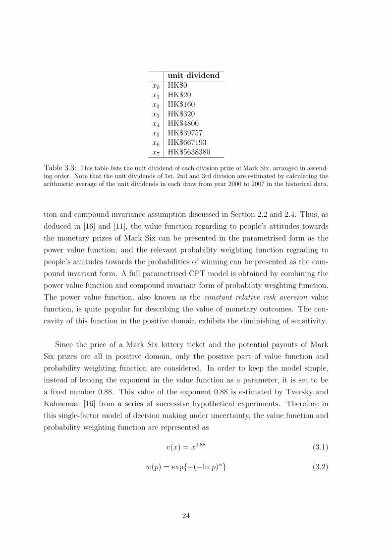
2.5 Plot of the function w(p) = exp{−β(−ln p)α} with fixed value of β =
1.5, α is 0.001, 0.25, 0.5, 0.75, 1, 1.5, 2, 5, 100. . . . . . . . . . . . . . . 19
2.6 Plot of the function w(p) = exp{−β(−ln p)α} with different values of
β = 0.5, 1, 1.5, α is fixed to be 0.65. . . . . . . . . . . . . . . . . . . . 20
2.7 Plot of the function w+(p) = w−(p) = exp{−(−ln p)α} with different
values of α within (0, 1). . . . . . . . . . . . . . . . . . . . . . . . . . 20
3.1 Plot of the probability weighting function w(p) = exp{−(−ln p)α} with
α = 0.93. . . . . . . . . . . . . . . . . . . . . . . . . . . . . . . . . . . 28
3.2 Magnified plot of the probability weighting function w(p) = exp{−(−ln p)α}with α = 0.93. . . . . . . . . . . . . . . . . . . . . . . . . . . . . . . . 28
3.3 Another magnified plot of the probability weighting function w(p) =
exp{−(−ln p)α} with α = 0.93. . . . . . . . . . . . . . . . . . . . . . 29
3.4 The surface plotted of the function f(σ, α) with parameter σ and α. . 32
3.5 Plot of the power value function v(x) = xσ with σ = 0.42. . . . . . . . 34
3.6 Plot of the probability weighting function w(p) = exp{−(−ln p)α} with
α = 0.70. . . . . . . . . . . . . . . . . . . . . . . . . . . . . . . . . . . 34
3.7 Plot of the probability weighting function w(p) = exp{−(−ln p)α} with
α = 0.70, for an extremely small interval near zero. . . . . . . . . . . 35
iii

iv

List of Tables
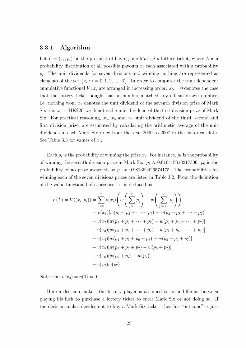
3.1 List of the criterion for awarding each division prize of Mark Six. . . . 22
3.2 List of the winning probabilities for each division prize of Mark Six. . 23
3.3 List of the unit dividend of each division of the Mark Six prize, arranged
in ascending order. . . . . . . . . . . . . . . . . . . . . . . . . . . . . 24
3.4 List of the averaged unit dividend of 1st, 2nd and 3rd division of the
Mark Six prize, with respect to the number of Jackpots before that draw. 30
3.5 List of residuals for each set of data, with σ = 0.42 and α = 0.70. . . 31
3.6 List of residuals for each set of data, with the parameters estimated by
Prelec . . . . . . . . . . . . . . . . . . . . . . . . . . . . . . . . . . . 33
v

vi

Chapter 1
Introduction
All the time people have to make decisions under uncertain conditions, about their
study, work or finance. The topic of decision making under uncertainty is unsurpris-
ingly studied for centuries by many disciplines, from mathematics, through finance
and economics to psychology. All these studies are concerned with how to define the
rationality, how to describe the logic behind decision making and people’s actual pref-
erences. The studies of decision making under uncertainty usually focus on two types
of choices: the risky choices involve possible losses, e.g. enter a gamble with specific
probabilities of winning and losing; and the riskless choices are normally referring to
an exchange of money for good or service.
1.1 Utility and Expected Utility Theory
A decision maker’s satisfaction or relative desirability to the possession or consump-
tion of wealth is measured in terms of utility. Economist used to distinguish between
cardinal utility and ordinal utility. Cardinal utility is a way to quantify the satisfac-
tion obtained by a person from good or service, hence its magnitude is meaningful.
While ordinal utility is a way to define an order, is a measure of preference. The
original idea of expected utility theory was discovered by Gabriel Cramer in 1728 [4]
and Daniel Bernoulli in 1738 [3] in order to solve the famous St. Petersburg paradox.
Bernoulli claimed that when making decisions under uncertainty in practice, people
tend not to maximise their expected monetary payoff but to maximise the expected
value of a logarithmic utility function. About two hundred years later, in 1944 von
Neumann and Morgenstern [10] published the axioms of expected utility theory in
their formulation of the game theory, consequently made the expected utility theory
1

become a fundamental and powerful tool for studying the decision making problems.
As formulated by von Neumann and Morgenstern [10], utility is described in terms
of a utility function. Let X = {x : x is a outcome} be a set of possible outcomes.
xi or x, y, z conventionally refer to the elements of X. A choice P = (xi, pi) is a
probability distribution defined on outcomes xi associated with probabilities pi. In
general, expected utility theory applies to any type of outcomes, money being a special
case. u : X → R denotes a utility function such that the value of u(x) is a measure
of the decision maker’s preference derived from the outcome x. The importance of a
utility function is that it derives a ranking, the actual magnitude is meaningless.
x � y ⇔ u(x) ≥ u(y) (1.1)
where x � y means the outcome x is preferred at least as much as the outcome y.
Equation (1.1) indicates clearly that the utility function is monotonic. Utility func-
tions are normally continuous and increasing since decision makers are assumed to
prefer more wealth to less. However, u(x) = x2 is not increasing for all values through
its domain, but it is still used quite often in some cases due to the tractability of this
function. The decrease of the function might somehow be employed to accommodate
the unacceptable outcome or satiation, e.g. one is sick of alcohol after drinking too
much.
In expected utility theory, decision makers’ attitudes towards uncertainty are
wholly modelled by the value of utility functions defined on final asset positions.
Every rational decision maker is assumed to make decisions following the principle of
maximising the value of his expected utility. The expected utility (EU) of a choice is
the sum of the utility functions of possible outcomes weighted by the corresponding
probabilities:
EU(P ) =∑i
piu(xi) (1.2)
Von Neumann and Morgenstern [10] stated in their expected utility theory that the
utility function exists if and only if the preferences satisfy four axioms: completeness,
transitivity, continuity and independence. The completeness axiom of preference says
that for any choice P,Q, we must have either P � Q, P � Q or P ∼ Q. The transitiv-
ity axiom of preference requires that if P � Q and Q � R, then P � R for any choice
P,Q and R. The continuity axiom of preference states that for any choice P � Q � R,
there exists a probability r ∈ [0, 1], such that Q ∼ rP + (1− r)R. Here rP +(1− r)R
2

is the single-stage equivalent of a compound two-stage choice in which P occurs with
probability r and R occurs with probability (1− r). The idea of continuity axiom is
that all choices of intermediate preference are preferred the same as some mixture of
a pair of better and worse choices. The independence axiom of expected utility theory
claims that if a decision maker prefers P at least as much as Q, then he must also
prefer rP +(1−r)R at least as much as rQ+(1−r)R, for any arbitrary choice R with
probability r. It basically says that the preference between two choices must be inde-
pendent of any common components. The independence axiom gives rise to the linear
structure of the expected utility, as EU(rP + (1− r)Q) = rEU(P ) + (1− r)EU(Q).
This linear structure in probabilities directly leads to the common consequence and
common ratio property. The common consequence property states that the prefer-
ence between two choices does not change if both choices are added or subtracted a
common outcome with same probability. The common ratio property states that the
preference between two choices does not change when probabilities in both choices are
multiplied by the same positive number, and the remaining probability is attached
to a common consequence [17]. However, the above four axioms underlying the ex-
pected utility theory have been intensely debated and questioned in the literature.
The violations of expected utility theory will be discussed in Section 1.2.
In implications of expected utility theory, the most significant assumption made
are the concavity of utility functions. Economically and financially, people are sup-
posed to be totally risk averse. Mathematically, concavity of a utility function means
∀ 0 ≤ α ≤ 1, x, y ∈ X, u(αx+ (1−α)y) ≥ αu(x) + (1−α)u(y). Where x is relatively
large, the small gradient of the concave utility function represents the diminishing of
marginal utility. If the derivative of the utility function u(·) is defined, concavity of
u(·) implies the decrease of u′(·). The explanation is that the decision maker who
is already very wealthy, obtains less additional satisfaction from each additional unit
of wealth. The degree of risk aversion is reflected by the shape of the utility func-
tion. The concavity and risk aversion assumption is seen as the main reason why
people spend the money in buying insurance premium, which eventually exceeds the
expected actuarial losses in accidents. However, most of time, most people do behave
in the way of obeying the axioms of expected utility theory [10].
3
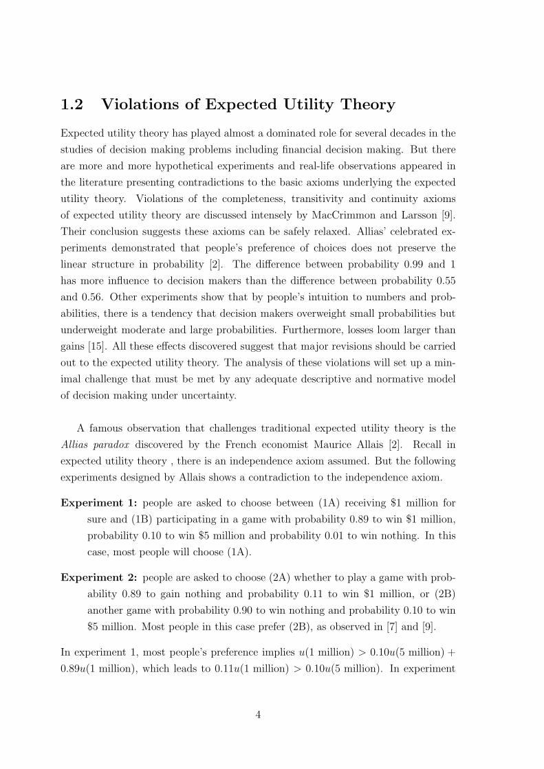
1.2 Violations of Expected Utility Theory
Expected utility theory has played almost a dominated role for several decades in the
studies of decision making problems including financial decision making. But there
are more and more hypothetical experiments and real-life observations appeared in
the literature presenting contradictions to the basic axioms underlying the expected
utility theory. Violations of the completeness, transitivity and continuity axioms
of expected utility theory are discussed intensely by MacCrimmon and Larsson [9].
Their conclusion suggests these axioms can be safely relaxed. Allias’ celebrated ex-
periments demonstrated that people’s preference of choices does not preserve the
linear structure in probability [2]. The difference between probability 0.99 and 1
has more influence to decision makers than the difference between probability 0.55
and 0.56. Other experiments show that by people’s intuition to numbers and prob-
abilities, there is a tendency that decision makers overweight small probabilities but
underweight moderate and large probabilities. Furthermore, losses loom larger than
gains [15]. All these effects discovered suggest that major revisions should be carried
out to the expected utility theory. The analysis of these violations will set up a min-
imal challenge that must be met by any adequate descriptive and normative model
of decision making under uncertainty.
A famous observation that challenges traditional expected utility theory is the
Allias paradox discovered by the French economist Maurice Allais [2]. Recall in
expected utility theory , there is an independence axiom assumed. But the following
experiments designed by Allais shows a contradiction to the independence axiom.
Experiment 1: people are asked to choose between (1A) receiving $1 million for
sure and (1B) participating in a game with probability 0.89 to win $1 million,
probability 0.10 to win $5 million and probability 0.01 to win nothing. In this
case, most people will choose (1A).
Experiment 2: people are asked to choose (2A) whether to play a game with prob-
ability 0.89 to gain nothing and probability 0.11 to win $1 million, or (2B)
another game with probability 0.90 to win nothing and probability 0.10 to win
$5 million. Most people in this case prefer (2B), as observed in [7] and [9].
In experiment 1, most people’s preference implies u(1 million) > 0.10u(5 million) +
0.89u(1 million), which leads to 0.11u(1 million) > 0.10u(5 million). In experiment
4

2, most people’s preference implies 0.10u(5 million) > 0.11u(1 million). So a contra-
diction between the traditional expected utility theory and common senses can be
spotted in this illustrative example. This effect is called common consequence effect
in the literature. This paradox presents the fact that some common sense towards
choices under uncertainty is not able to be fully captured by the expect utility model.
Efforts trying to adjust the independence axiom of expected utility theory led to the
discovery of prospect theory [7] discussed in Section 1.3.
Another paradox illustrates the so-called common ratio effect is also originally
designed by Allais [2].
Experiment 1: people are asked to choose between (1A) receiving $3000 for sure
and (1B) participating in a game with probability 0.80 to win $4000, probability
0.20 to win nothing. Most people in this case choose (1A).
Experiment 2: people are asked to choose (2A) whether to play a game with prob-
ability 0.25 to gain $3000 and probability 0.75 to win nothing, or another game
(2B) with probability 0.20 to win $4000 and probability 0.80 to win nothing.
As in Allais’ experiment, most people in this case prefer (2B).
By calculating the expected utility, the preference of most people in Experiment 1
implies 0.8u(4000) < u(3000). But in Experiment 2, the preference of most people
implies 0.25u(3000) < 0.20u(4000) which further implies u(3000) < 0.8u(4000). This
contradicts the expected utility theory but not common sense. This common ratio
effect is used by Prelec [11] as a building block in developing his compound invariant
form of probability weighting function.
It is widely agreed that the expected utility theory is not sufficient to be an ade-
quate or accurate model for studying decision making under uncertainty. Evidences
suggest that the final state of wealth are not always important for decision making
[1]. People intuitively separate the outcomes into gains and losses according to some
chosen reference point. The reference point is derived from choices presented and
decision maker’s personal expectation. Assigning values to gains and losses distinc-
tively is one way to address this issue. This idea plays a central role in Kahneman
and Tversky’s treatment of choices in their prospect theory [7].
However people’s decisions also depend on how they frame the decision making
problem, i.e. not only how they distinguish the gains and losses, but also how they
5

treat potential gains and losses. Therefore, another feature should be considered
is to assign different weights to gains and losses. People’s preference to a choice
depends not only on the probabilities of the possible outcomes but also the relatively
desirability of one possible outcome in comparison to the other possible outcomes. In
general people take possible losses more seriously than gains, hence people choose to
avoid possible losses rather than seek for possible gains [15]. People tend to overweight
extreme events with extremely small probabilities and to underweight average events
with large probabilities. The fourfold pattern of risk attitudes summarises the rules of
decision making: people are risk averse for gains accompanying large probability; risk
averse for losses accompanying small probability; risk seeking for gains accompanying
small probability; risk seeking for losses accompanying large probability.
1.3 Prospect Theory
Expected utility theory is not always consistent with people’s intuition, and some
people even systematically violate the axioms underlying the expected utility theory.
In order to build a more adequate model for decision making under uncertainty, many
authors derived various generalised models from empirical data, axiomatic generalisa-
tions, and intuition about choices [17]. Prospect Theory was proposed by Markowitz
[8] and strengthened by two extraordinary psychologists Kahneman and Tversky [7].
In prospect theory, the choices people have to make decisions on, are described as
prospects. As defined by Kahneman and Tversky [7], a prospect (xi, pi) is a contract
that yields outcome xi associated with probability pi, where the sum of pi is 1.
In the prospect theory model, decision makers are assumed first to edit the choices
in order to simplify the evaluation of choices; then they make decisions according to
the evaluation. In the evaluation phase, a value function and a nonlinear transforma-
tion of the probability scale is embounded. Instead of considering the utility function
on final asset positions, the value function v(x), which mimics the idea of utility func-
tion but is defined on the current asset position, measures the value of deviation from
the reference point, i.e. gains and losses. Probability weighting function w(p) replaces
the cumulative probabilities. By assigning probability weighting function to each
probability, the overall impact of the probabilities on the decision can be controlled
more sensibly. A monotonic transformation1 is employed against the original prob-
ability scale, thus to overweight small probabilities and underweight moderate and
1transform a set of numbers into another set so that the ranking of the original set is preserved.
6

large probabilities. This preformed model of prospect theory is managed to explain
some major violations of expected utility theory, with respect to a small number of
outcomes. However, there are also some issues raised in this early version of prospect
theory. It does not always satisfy the stochastic dominance2; it is not compatible
with large number of outcomes; the source of uncertainty is not distinguished.
1.4 Cumulative Prospect Theory
Based on the earlier version of prospect theory, many authors have proposed more
advanced and generalised models for decision making under uncertainty. For instance,
the Anticipated Utility Model designed by Quiggin [13] and the Choquet Expected
Utility model discovered by Wakker [18] managed to apply the cumulative utility to
decision making problem, hence explained some of the major behaviours observed in
various paradoxes. However, in this project the idea of Cumulative Prospect Theory
(CPT) developed by Tversky and Kahneman [16] is adapted and analysed. As an im-
provement and variant of their earlier version of prospect theory, cumulative prospect
theory incorporates many recent developments in this area. It is an adequate, de-
scriptive and normative model for decision making under uncertainty. CPT model
transforms probabilities of outcomes cumulatively rather than individually. It can be
utilised to any uncertain prospects with even continuous probability distributions and
unlimited number of outcomes. This model also enables to treat different probability
weighting functions for gains and losses respectively. Thus it can accommodate some
form of source dependence. More importantly, CPT model satisfies the stochastic
dominance. Due to Daniel Kahneman’s contribution to behavioural economics and
the development of CPT, he was awarded the Sveriges Riksbank Prize in Economic
Sciences in Memory of Alfred Nobel in 2002, “for having integrated insights from
psychological research into economic science, especially concerning human judgment
and decision-making under uncertainty” [22].
1.5 Aim of the Project
Drazen Prelec [11] relied on the common ratio effect as a building block to introduce
an alternative way of parametrising the probability weighting functions by considering
2if P ((−∞, τ ]) ≤ Q((−∞, τ ]) for all τ ∈ R, then P is called to stochastically dominate Q.
7

the compound invariance of prospects. The compound invariant form of probability
weighting function requires less axioms, is easy to estimate with the capabilities to
explain all the major characteristics of decision making under uncertainty. The aim
of this project is to estimate the parameters in a full parametrised CPT model. The
model combines the power value function, and the compound invariant form of prob-
ability weighting function designed by Prelec. Unlike in the literature the parameters
are estimated from artificial and hypothetical surveys or experiments, in this project
the data obtained from Hong Kong Mark Six lottery market is used for calibration.
Therefore the curvature of functions and performance of the model in the real-life
situation can be examined.
In modelling people’s preferences in lottery market, it is assumed that in general,
lottery players are indifferent in buying the lottery ticket to enter the game or not
doing so. Then according to this relation, two models of decision making under
uncertainty are constructed. In the single-factor case, the exponent of power value
function is fixed with the value suggested by Tversky and Kahneman, the parameter
in the probability weighting function need to be estimated from the data. While in the
two-factor case, the least squares estimation is employed to obtain both parameters
in the value function and probability weighting function. Therefore we can examine
the properties of these models, and how these models fit people’s behaviours when
making decisions under uncertainty.
1.6 Organisation of the Dissertation
In this introductory chapter, how the problem of decision making under uncertainty
is formulated in the literature, is reviewed. The axiomisation of cumulative prospect
theory and the compound invariant form of probability weighting function are pre-
sented in Chapter 2. The explicit parametrised form of value functions and probability
weighting functions are given in Section 2.3 and 2.4. The rule of Hong Kong Mark Six
lottery game and the data used in this project are explained in details in Section 3.1
and 3.2. Then a single-factor model and a two-factor model are constructed and the
parameters are estimated in Section 3.3 and 3.4. The performance of these models
regarding to the lottery game is discussed in Section 3.3.2 and 3.4.2 respectively.
8

Chapter 2
Theoretical Framework
2.1 Cumulative Presentation of Uncertainty
Cumulative prospect theory distinguishes two phases during the decision making pro-
cess, namely the framing phase and the evaluation phase. In the framing phase, the
given choices and their outcomes are reformulated into some form of representation,
by decision makers according to their own views of gains, losses and uncertainty.
Although there is no unified theory of how decision makers edit the choices, but a
considerable amount of rules which govern the behaviour have been obtained in the
literature [14]. The framing phase is followed by the evaluation phase. In the evalua-
tion phase, the value of each prospect is analysed and computed by decision makers.
Decisions are then made among choices accordingly.
The following definitions and representations are based on the work of Tversky
and Kahneman [16]. Recall the definitions in the introduction part, X is the set of
possible outcomes. xi and x, y, z conventionally refer to the elements of the set. Each
outcome can have either positive value or negative value. Since in this project only
monetary outcomes are considered, the reference point is 0. Thus the actual amount
of money received or paid become gains or losses. S is introduced as a finite state
space, each subset of S is called an event. A prospect is a function f : S → X assigns
to each event s ∈ S an outcome x ∈ X. A prospect is called positive or negative if
the relevant outcomes are positive or negative. f+(s) = f(s) if f(s) > 0, f+(s) = 0
if f(s) ≤ 0, the negative part is defined similarly. Let Ai be a partition of the set
S, (xi, Ai) is interpreted as xi is the outcome while Ai occurs. A prospect f then
becomes a sequence of pairs (xi, Ai) with xi arranged in ascending order. The value
function v : X → R measures the value of gains and losses, v(0) = 0. A cumulative
9

functional V is defined as f � g ⇔ V (f) ≥ V (g). Similar to the idea of utility func-
tion in expected utility theory, V is defined on the prospects while v is defined on the
outcomes. W is called the capability which is a function that assigns to each A ⊂ S
a number W (A) satisfying W (φ) = 0 and W (S) = 1, A ⊃ B ⇒ W (A) ≥ W (B).
The decision weight for an outcome, π(x), which represents the marginal contri-
butions to the events, is defined in terms of W+ and W−. So for positive outcome,
π+i can be interpreted as the difference of the capacities between the events: “the
outcome is preferred at least the same as xi in every respect” and “the outcome is
more preferred than xi in at least one respect”. Similarly, the decision weight for
negative outcome, π−i can be interpreted as the difference of the capacities between
the events: “the outcome is preferred at least the same as xi in every respect”’ and
“the outcome is less preferred than xi in at least one respect”.
π+i = W+(Ai ∪ · · · ∪ An)−W+(Ai+1 ∪ · · · ∪ An) , 0 ≤ i ≤ n− 1
π−i = W−(A−m ∪ · · · ∪ Ai)−W−(A−m ∪ · · · ∪ Ai−1) , 1−m ≤ i ≤ 0
π+n = W+(An) , π−−m = W−(A−m)
n∑i=0
π+i = 1 ,
0∑i=−m
π−i = 1
Hence the value of a prospect V (f) = V ((xi, Ai)) can be written as, for −m ≤i ≤ n,
V (f) = V (f+) + V (f−) =n∑
i=−m
πiv(xi) (2.1)
V (f+) =n∑i=0
π+i v(xi)
V (f−) =0∑
i=−m
π−i v(xi)
If each capability W is additive, then W turns to be a probability measure. Let Pbe a set of probability distributions defined on the set X. Hence the prospect can be
formulated as a finite probability distribution over outcomes. P+ and P− correspond
to the positive and negative parts of X. The preference relation is represented by
P � Q ⇔ V (P ) � V (Q) for all P , Q in P . w(pi) is the probability weighting
function assigning weight to the outcome. w+ and w− correspond to the positive and
10

negative outcomes. w+ and w− are strictly increasing functions, w+(0) = w−(0) = 0,
w+(1) = w−(1) = 1. Then in this case, decision weights are defined as
π+i = w+(pi + · · ·+ pn)− w+(pi+1 + · · ·+ pn) , 0 ≤ i ≤ n− 1
π−i = w−(p−m + · · ·+ pi)− w−(p−m + · · ·+ pi−1) , 1−m ≤ i ≤ 0
π+n = w+(pn) , π−−m = w−(p−m)
Note that it is assumed w+(p) = w−(p) . If w−(p) = 1 − w+(1 − p), we get
a pure rank dependent model. See [7], [16] and [11] for details. Thus a prospect
P = (x1, p1; . . . ;xn, pn) for x1 ≤ · · · ≤ xm ≤ 0 ≤ xm+1 ≤ · · · ≤ xn, can be written
explicitly as
V (P ) =m∑i=1
v(xi)
(w−
(i∑
j=1
pj
)− w−
(i−1∑j=1
pj
))
+n∑
i=m+1
v(xi)
(w+
(n∑j=i
pj
)− w+
(n∑
j=i+1
pj
))(2.2)
Therefore, a simple prospect (0, 1 − p;x, p), which is conventionally abbreviated
as (x, p), can be written in a separable form as
V ((x, p)) =
{w+(p)v(x), x > 0
w−(p)v(x), x < 0(2.3)
A binary prospect (x, p; y, q) is an abbreviation for the prospect (0, 1 − p −q;x, p; y, q), where 0 < x < y or y < x < 0. If 0 < x < y, a binary prospect
can be interpreted as the decision maker can gain the outcome x with probability
(p+q) and a further (y−x) with probability q. If y < x < 0, then the decision maker
would lose x with probability (p + q) and a further (y − x) with probability q. So a
binary prospect can be written as
V ((x, p)) =
w+(p+ q)v(x) + w+(q)(v(y)− v(x)), 0 < x < y
w−(p+ q)v(x) + w−(v(y)− v(x)), y < x < 0
w−(p)v(x) + w+(q)v(y), x < 0 < y
(2.4)
The general form of the value of a prospect, which allows the treatment for arbi-
trary continuous outcomes is in the form of the following,
V (P ) =
∫R+
v(x)d
dx(w+(G(x, p))) dx+
∫R−
v(x)d
dx(w−(G(x, p))) dx (2.5)
where G(x, p) :=∫ x−∞ dp is the cumulative probability [20].
11
2.2 Axiomisation of CPT
To formulate the cumulative prospect model, some axioms need to be understood
at the first place. Note that in CPT, the decision maker is assumed to be indiffer-
ent between receiving a payoff x and x + y but returning y. The following axioms
are systematically summarised by Wakker and Tversky [19], Wakker [20] and Prelec
[11]. Preference relations and prospects are assumed to satisfy the following without
restrictions:
• Weak Ordering: the same as in expected utility theory, the preference relation is
complete, i.e. there must exist P � Q, P � Q or P ∼ Q for any prospect P,Q;
the preference relation is transitive, i.e. P � Q and Q � H implies P � H.
• Strict Stochastic Dominance: P > Q if P 6= Q and P stochastically dominates
Q. Recall the definition of stochastic dominance, if P ((−∞, τ ]) ≤ Q((−∞, τ ])
for all τ ∈ R, then P is called to stochastically dominate Q. Notice that stochas-
tical dominance is weak ordering.
• Certainty Equivalent Condition: there exits an outcome x such that (x) ∼ P for
any P . (x) is the abbreviation for (x, 1) which means there is only one outcome
x with 100% certainty p = 1.
• Continuity in Probability: if (x, p) ≺ (y) for fixed p ∈ (0, 1), then there exists
q and r, q < p < r, (x, q) ≺ (y) and (x, r) ≺ (y). The same holds if the two
preferences and inequalities are reversed.
• Tradeoff Consistency: let �∗ be a quaternary preference relation, XY �∗ X ′Y ′
is defined for outcomes X , Y , X ′ and Y ′ as if
(x1, p1; . . . ;X , pi; . . . ;xn, pn) � (y1, p1; . . . ;Y , pi; . . . ; yn, pn) and
(x1, p1; . . . ;X ′, pi; . . . ;xn, pn) � (y1, p1; . . . ;Y ′, pi; . . . ; yn, pn)
Then by substituting CPT for above prospects, the following inequality is im-
plied accordingly,
u(X )− u(Y) ≥ u(X ′)− u(Y ′)
Therefore, the preference relation � satisfies the tradeoff consistency if XY �∗
X ′Y ′ and XY ≺∗ X ′Y ′ are not satisfied simultaneously by the same X , Y , X ′
and Y ′. The details about tradeoff consistency can be found in [20].
12

• Simple Continuity: consider rank ordered n tuples (k, n) extracted from the set
X, where 0 ≤ k ≤ n, then S(k, n) := {(x1, . . . , xn) ∈ Xn : x1 ≤ · · · ≤ xk ≤0 ≤ xk+1 ≤ · · · ≤ xn}. Therefore the preference relation satisfies the simple
continuity condition, if for any probability vector (p1, . . . , pn) the preference
induced on each S(k, n) is continuous.
The above axioms will be called fundamental axioms in the following chapters
of this project. By Theorem 6.3 in [19], the fundamental axioms ensure that CPT
holds with all capacities uniquely determined, in other words, with unique and non-
decreasing w+(p), w−(p) satisfying w+(0) = w−(0) = 0 and w+(1) = w−(1) = 1; and
the value function is a ratio scale. Furthermore, Theorem 12 in [20] indicated that
above axioms actually imply the probability weighting function is strictly increasing
on [0, 1] and continuous on (0, 1). Even the probability weighting function is continu-
ous on [0, 1], if the continuity in probability axiom is replaced by boundary continuity.
2.3 Values and Weights
In cumulative prospect theory, a decision maker’s risk seeking or risk aversion is de-
termined by joining the value function and the probability weighting function. As
mentioned previously, the value function is defined on gains and losses. Psychologi-
cally, the difference in value between gaining $200 and $400 appears greater than the
difference between gaining $3200 and $3400. The difference in value between losing
$200 and $400 appears greater than the difference between losing $3200 and $3400.
This phenomena is called principle of diminishing sensitivity. Therefore the value
function v is assumed to be concave above the reference point 0 and convex below 0,
thus S shaped. Kahneman and Tversky’s analysis based on empirical data confirmed
this result [7]. Concavity of the value function implies v′′(x) < 0 for all x > 0, while
convexity implies v′′(x) > 0 for all x < 0. The gradient of v is assumed to be steeper
for losses than for gains, v′(x) < v′(−x) for all x > 0. Because losses loom larger
than corresponding gains, according to the principle of loss aversion [15].
Investigations show that most people prefer a sure gain rather than a gamble, while
most people prefer a gamble rather than a sure loss [5]. The principle of diminishing
sensitivity also exists among probability weighting functions, since the impact of a
given change in probability diminishes with its distance from the boundary. Conse-
quently the probability weighting function should be concave near 0 and convex near
13

Figure 2.1: Plot of the value function v(x) as in equation (2.6) with α = β = 0.88 and λ = 2.25.
1, hence an inverse S shaped. Therefore, the overweight of small probabilities con-
sequently leads to the attraction of small probability gains and aversion of the small
probability losses. While underweight of large probabilities consequently diminishes
the attraction of large probability gains and aversion of large probability losses. To
summarise the results obtained as in [7], the probability weighting function is increas-
ing in p; discontinuous at 0 and 1; w(0) = 0 and w(1) = 1; w(p) > p for small p; w(p)
is subadditive for small p, i.e. w(rp) > rw(p) for 0 ≤ r ≤ 1; w(p) is subproportional,
i.e. w(pq)/w(p) < w(pqr)/w(pr); and w(p) is subcertain, i.e. w(p) + w(1 − p) < 1.
In [16], Tversky and Kahneman further claimed that the probability weighting func-
tions are inverse S shaped, concave around probability 0 and convex near probability
1; probability weighting functions are reflective, w+(p) = w−(p), which means equal
weight is assigned to a gain as to a loss; probability weighting functions are asymmet-
rical with a fixed point at about 0.37, which is below 0.5, the weight of uncertainty
related to certainty is further decreased; probability weighting functions are regres-
sive, the curve of a probability weighting function intersects the diagonal from above,
this property reflects the fourfold pattern of risk attitudes mentioned in Section 1.2.
Tversky and Kahneman gave the explicit functions for value and weights, they
also estimate the parameters from a series of systematical experiments [16]. The pa-
14

Figure 2.2: Plot of the probability weighting functions w+(p) = pγ
(pγ+(1−p)γ)1/γand w−(p) =
pδ
(pδ+(1−p)δ)1/δ with γ = 0.61 and δ = 0.69.
rameters α and β are both estimated to be 0.88. The median value of λ is 2.25. γ
and δ approximately equals 0.61 and 0.69 respectively. The following functions with
estimated parameters are plotted as Figure 2.1 and 2.2. We can see from the plots
that they satisfy all the characteristics observed for value function and probability
weighting function.
v(x) =
{xα, x ≥ 0
−λ(−x)β, x < 0(2.6)
and
w+(p) =pγ
(pγ + (1− p)γ)1/γ(2.7)
w−(p) =pδ
(pδ + (1− p)δ)1/δ(2.8)
2.4 Compound Invariant Weighting Functions
Recall the common ratio effect described in Section 1.2, this effect is explained by
Kahneman and Tversky [7] to assume log(w(p)) is convex in log(p). Mathemati-
cally, the common ratio effect says that ∀ 0 < λ < 1, p 6= q,(x, p) ∼ (y, q) implies
15
(y, λq) � (x, λp) for 0 < x < y, or (y, λq) ≺ (x, λp) for y < x < 0. This is called the
subproportionality of prospects [7]. Drazen Prelec [11] proposed the compound invari-
ant form of probability weighting function in order to explain common ratio effect
more thoroughly and fulfil the three empirical requirements of probability weighting
function: the under/overweighting, subproportionality and subadditivity.
For any outcome x, y, x′, y′, with corresponding probabilities p, q, r, s ∈ [0, 1],
and compounding integer N ∈ N, N ≥ 1, if (x, p) ∼ (y, q) and (x, r) ∼ (y, s), then
(x′, pN) ∼ (y′, qN) ⇒ (x′, rN) ∼ (y′, sN). It is the compound invariance condition
satisfied by preference relations. The assumption and following parametrised func-
tions were introduced and rigorously proved by Prelec [11]. Compound invariance
assumption can be seen as an implication of expected utility theory but it is a much
weaker condition. It aligns all three requirements for probability weighting function.
Given the assumption, the over/underweighting, subproportionality and subadditiv-
ity of probability weighting function coincide.
In the context of CPT, if the fundamental axioms and compound invariance as-
sumption are satisfied, the probability weighting functions for gains and losses, can
be represented as
w+(p) = exp{−β+(−ln p)α}
w−(p) = exp{−β−(−ln p)α} (2.9)
where 0 < α < 1 is unique, β+ > 0, β− > 0.
Here are some special cases of the equation (2.9):
• If α = β+ = β− = 1, the probability weighting functions become linear, w+(p) =
w−(p) = p. The expected utility theory is recovered.
• If α = 1, β+ > 0, β− > 0, the probability weighting functions become
w+(p) = pβ+
w−(p) = pβ−
In this case, the probability weighting functions are not linear. But obviously
these power functions do not satisfy any of the empirical requirements.
• If α > 1, β+ > 0, β− > 0, the plot of the functions gives an S shape, convex
followed by concave.
16
• If 0 < α < 1, β+ > 0, β− > 0, the plot of the probability weighting func-
tions shows an inverse S shape, they intersect the diagonal from above, initially
concave then convex, and are subproportional.
These obsevations are evidenced from Figure 2.3, 2.4 and 2.5. Also Figure 2.6 in-
dicates that in equation (2.9), as β increases, the probability weighting functions
become more convex, but still remain subproportional and inverse S shaped.
As claimed by Prelec [11], preferences P and Q are called quasiconcave if P ∼Q⇒ Q � λP + (1−λ)Q, for any λ ∈ [0, 1]. Similarly P and Q are called quasiconvex
if P ∼ Q ⇒ Q � λP + (1 − λ)Q. If Q is a certain prospect, then certainty-
equivalent-quasiconcave (CE-quasiconcave) and certainty-equivalent-quasiconvex are
defined accordingly. Consider a set of binary prospects where the probability of
extreme outcome is at least s and the probability of gaining nothing is at least 1− r,∆+[s, r] = {(x, p; y, q) : 0 < x < y, s ≤ q, p + q ≤ r} and ∆−[s, r] = {(x, p; y, q) :
y < x < 0, s ≤ q, p + q ≤ r}. Strict CE-quasiconcave on ∆+[s, r] means P ∼Q ⇒ Q � λP + (1 − λ)Q for any certain prospect Q. Diagonal Concavity says
there is no non degenerate interval [s, r] such that � is quasiconvex and strict CE-
quasiconcave on ∆+[s, r] or ∆−[s, r], nor quasiconcave and strictly CE-quasiconvex
on ∆+[s, r] or ∆−[s, r]. Observations so far show that probability weighting function
is concave where the probability is overweighted and convex where the probability is
underweighted. Thus it agrees that a subproportional probability weighting function
is diagonally concave.
In the context of CPT, if the fundamental axioms, compound invariance assump-
tion and diagonal concavity condition are satisfied by preferences, the probability
weighting function can be characterised in the form
w+(p) = w−(p) = exp{−(−ln p)α} (2.10)
where 0 < α < 1 is unique. Figure 2.7 is a plot for equation (2.10). It is clearly that
for all possible values of α in the range from 0 to 1, the probability weighting function
intersects the diagonal from above; the probability weighting function is concave be-
fore intersecting the diagonal and convex beyond the diagonal. Hence the probability
weighting function is regressive and S shaped. The convex region is about twice as
large as the concave region. The probability weighting function is asymmetric at a
fixed point p = 1/e = 0.37.
17
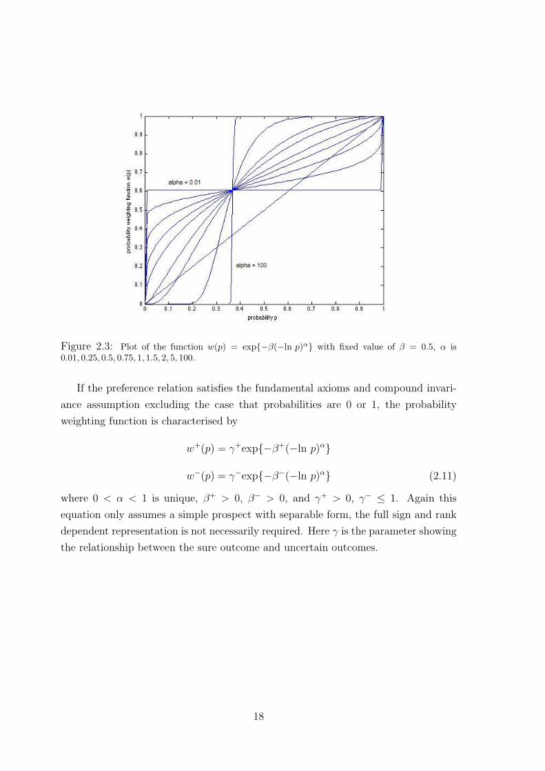
Figure 2.3: Plot of the function w(p) = exp{−β(−ln p)α} with fixed value of β = 0.5, α is0.01, 0.25, 0.5, 0.75, 1, 1.5, 2, 5, 100.
If the preference relation satisfies the fundamental axioms and compound invari-
ance assumption excluding the case that probabilities are 0 or 1, the probability
weighting function is characterised by
w+(p) = γ+exp{−β+(−ln p)α}
w−(p) = γ−exp{−β−(−ln p)α} (2.11)
where 0 < α < 1 is unique, β+ > 0, β− > 0, and γ+ > 0, γ− ≤ 1. Again this
equation only assumes a simple prospect with separable form, the full sign and rank
dependent representation is not necessarily required. Here γ is the parameter showing
the relationship between the sure outcome and uncertain outcomes.
18
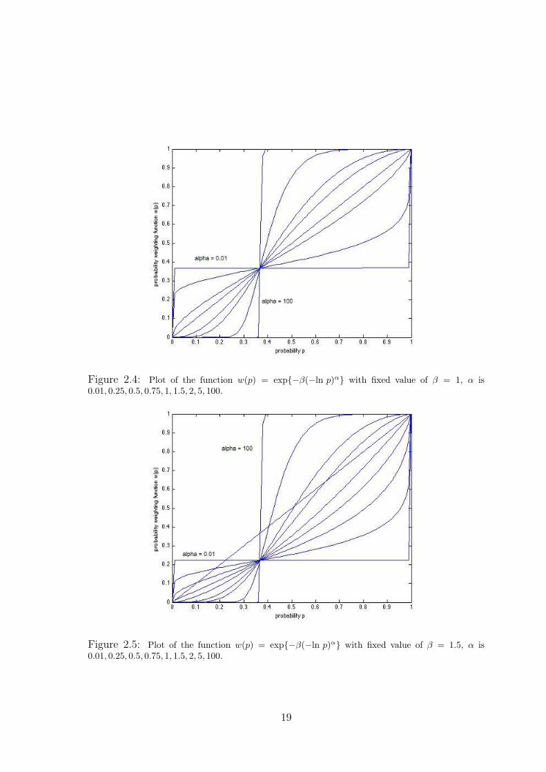
Figure 2.4: Plot of the function w(p) = exp{−β(−ln p)α} with fixed value of β = 1, α is0.01, 0.25, 0.5, 0.75, 1, 1.5, 2, 5, 100.
Figure 2.5: Plot of the function w(p) = exp{−β(−ln p)α} with fixed value of β = 1.5, α is0.01, 0.25, 0.5, 0.75, 1, 1.5, 2, 5, 100.
19

Figure 2.6: Plot of the function w(p) = exp{−β(−ln p)α} with different values of β = 0.5, 1, 1.5,α is fixed to be 0.65.
Figure 2.7: Plot of the function w+(p) = w−(p) = exp{−(−ln p)α} with different values of αwithin (0, 1).
20

Chapter 3
Numerical Experiment
3.1 Mark Six
Mark Six is a lottery game founded and organised by the Hong Kong Jockey Club.
Player pays HK$5 to purchase a lottery ticket with one selection of six numbers among
1 to 49 to enter Mark Six. On the draw day, the drawing process is broadcasted live
and famous people are invited to monitor the process to ensure the fairness. A lot-
tery machine which is a transparent sphere, draws numbered lottery balls out. Each
lottery ball is painted with different colours and numbers from 1 to 49. The lottery
machine is rolling during the drawing process to ensure the randomness. Seven num-
bers are successively drawn out from the machine, first six of the numbers are called
drawn numbers with last one called the extra number.
The awarding criterion and prizes of seven divisions are listed in Table 3.1. Ac-
cording to the regulations of Mark Six edited by HKJC [21], the first division prize is
awarded if any selection of six numbers are exactly the same as all six drawn numbers
regardless of the order. The second division prize is awarded if any selection of six
numbers are the same as five of the drawn numbers plus the extra number. 54% of
the sales revenue of Mark Six is distributed into a prize fund for funding prizes. The
payouts for each winning unit in the fourth, fifth, sixth and seventh division are fixed
to be HK$4800, HK$320, HK$160 and HK$20. They are first deducted from the prize
fund. In each draw, 7% of sales income is kept into a Snowball pool. In the draws
on some special days like Chinese New Year or Christmas Day, the money in the
Snowball pool will be added to the first division prize. Then the prizes for the first,
second and third division are dependent on percentages of the remainder of the prize
fund, the existence of Jackpot and the Snowball. The prize for the first division is
guaranteed no less than HK$5 million. The prize for the first division should at least
21

Criteria PrizeAll 6 drawn numbers 45% of the remainder of prize fund, and Jockpot,
Snowball. Guaranteed no less then HK$5 million5 drawn numbers and the extra number 15% of the remainder of prize fund5 drawn numbers 40% the remainder of prize fund4 drawn numbers and the extra number HK$48004 drawn numbers HK$3203 drawn numbers and the extra number HK$1603 drawn numbers HK$20
Table 3.1: The awarding criterion and prizes for seven divisions of prize in Mark Six. Note thatthe 3rd division is allocated a larger proportion of the prize fund than the 2nd division, becausethere are usually more winning units sharing the 3rd division prize, so the actual unit dividend in3rd division is much smaller than in 2nd division.
double the prize for the second division; the prize for the second division should at
least double the prize for the third division which should at least double the prize of
the fourth division. If more than one lottery ticket meet the awarding criterion, the
prize is shared among the winning units. If no one wins the first or second division
prize, the awarding money will be placed into a Jackpot. Then in the successive draw,
the first division prize winner gets the awarding for the present draw and the money
in the Jackpot.
3.2 Data
The data is constructed based on the statistics from Hong Kong Mark Six lottery
market. Three pieces of information is collected for each Mark Six lottery draw dated
from 2000 to 2007, a period of seven years. The first piece of data is the payouts to
each winning unit of the seven different divisions of prizes, namely the unit dividends.
The second piece of data is the number of winning units of each division in each draw.
The price for a Mark Six ticket used to be HK$2 and HK$4, some loyal players are
still allowed to buy lottery tickets with these prices. So when calculating the number
of winning units, if the lottery ticket is bought with, e.g. HK$2, then it is counted
to be 0.4 unit. The lottery player who spends HK$2 on a Mark Six ticket can only
be awarded 40 percent of any unit dividend if he wins. Thereby the statistics of the
winning units frequently shows not integers but numbers with one decimal place. Fi-
nally the total turnover of the lottery ticket sales for each draw is recorded. There is
a clear trend that the amount of total turnover becomes very large, when the amount
22

Division of Prize Winning Probability1st 1
(496 )≈ 7.1511238× 10⁻⁸
2nd(65)
(496 )≈ 42.9067431× 10⁻⁸
3rd(65)(
421 )
(496 )≈ 1802.0842907× 10−8
4th(64)(
421 )
(496 )≈ 4505.2147861× 10−8
5th(64)(
422 )
(496 )≈ 92356.5702464× 10−8
6th(63)(
422 )
(496 )≈ 123142.0936619× 10−8
7th(63)(
433 )
(496 )≈ 1641901.3217306× 10−8
Table 3.2: The winning probabilities for each division prize of Mark Six. All figures are accurateto the seventh decimal places.
of money kept in the Jackpot becomes very large. As there are more people buying
lottery tickets to enter Mark Six expecting for larger payouts.
The first reason I choose lottery data for analysing the decision making models,
is that the lottery game draws winners from a pool of an enormous amount of par-
ticipants. Very few of lottery players are believed to have knowledge about decision
making theory, so the behaviours observed are believed to be identical and realis-
tic. In contrast, most of the similar experiments in the literature are artificially or
hypothetically designed. The data is systematically obtained from a small group of
people, thus the results are less convincing. The second reason is that the lottery
players in Mark Six are obviously bearing an extremely large scale of risk of losing a
small amount of entrance fee, but expecting an extremely small probability of win-
ning a huge amount of prize. Prelec’s representation of probability weighting function
is mainly designed for the purpose of studying decision making problems under ex-
tremely small probabilities, so the lottery data is ideal for analysing the fitting and
performance of his model.
3.3 Single-Factor Model
In the Hong Kong Mark Six lottery market, it is assumed that the prospect of having
a Mark Six lottery ticket satisfies the fundamental axioms, diagonal concavity condi-
23
unit dividendx0 HK$0x1 HK$20x2 HK$160x3 HK$320x4 HK$4800x5 HK$39757x6 HK$667193x7 HK$5638380
Table 3.3: This table lists the unit dividend of each division prize of Mark Six, arranged in ascend-ing order. Note that the unit dividends of 1st, 2nd and 3rd division are estimated by calculating thearithmetic average of the unit dividends in each draw from year 2000 to 2007 in the historical data.
tion and compound invariance assumption discussed in Section 2.2 and 2.4. Thus, as
deduced in [16] and [11], the value function regarding to people’s attitudes towards
the monetary prizes of Mark Six can be presented in the parametrised form as the
power value function; and the relevant probability weighting function regrading to
people’s attitudes towards the probabilities of winning can be presented as the com-
pound invariant form. A full parametrised CPT model is obtained by combining the
power value function and compound invariant form of probability weighting function.
The power value function, also known as the constant relative risk aversion value
function, is quite popular for describing the value of monetary outcomes. The con-
cavity of this function in the positive domain exhibits the diminishing of sensitivity.
Since the price of a Mark Six lottery ticket and the potential payouts of Mark
Six prizes are all in positive domain, only the positive part of value function and
probability weighting function are considered. In order to keep the model simple,
instead of leaving the exponent in the value function as a parameter, it is set to be
a fixed number 0.88. This value of the exponent 0.88 is estimated by Tversky and
Kahneman [16] from a series of successive hypothetical experiments. Therefore in
this single-factor model of decision making under uncertainty, the value function and
probability weighting function are represented as
v(x) = x0.88 (3.1)
w(p) = exp{−(−ln p)α} (3.2)
24
3.3.1 Algorithm
Let L = (xi, pi) be the prospect of having one Mark Six lottery ticket, where L is a
probability distribution of all possible payouts xi each associated with a probability
pi. The unit dividends for seven divisions and winning nothing are represented as
elements of the set {xi : i = 0, 1, 2, . . . , 7}. In order to computer the rank dependent
cumulative functional V , xi are arranged in increasing order. x0 = 0 denotes the case
that the lottery ticket bought has no number matched any official drawn number,
i.e. nothing won; x1 denotes the unit dividend of the seventh division prize of Mark
Six, i.e. x1 = HK$20; x7 denotes the unit dividend of the first division prize of Mark
Six. For practical reasoning, x5, x6 and x7, unit dividend of the third, second and
first division prize, are estimated by calculating the arithmetic average of the unit
dividends in each Mark Six draw from the year 2000 to 2007 in the historical data.
See Table 3.3 for values of xi.
Each pi is the probability of winning the prize xi. For instance, p1 is the probability
of winning the seventh division prize in Mark Six, p1 ≈ 0.016419013217306. p0 is the
probability of no prize awarded, so p0 ≈ 0.981362426574175. The probabilities for
winning each of the seven divisions prizes are listed in Table 3.2. From the definition
of the value functional of a prospect, it is deduced as
V (L) = V ((xi, pi)) =7∑i=0
v(xi)
(w
(7∑j=i
pj
)− w
(7∑
j=i+1
pj
))= v(x1)[w(p1 + p2 + · · ·+ p7)− w(p2 + p3 + · · ·+ p7)]
+ v(x2)[w(p2 + p3 + · · ·+ p7)− w(p3 + p4 + · · ·+ p7)]
+ v(x3)[w(p3 + p4 + · · ·+ p7)− w(p4 + p5 + · · ·+ p7)]
+ v(x4)[w(p4 + p5 + p6 + p7)− w(p5 + p6 + p7)]
+ v(x5)[w(p5 + p6 + p7)− w(p6 + p7)]
+ v(x6)[w(p6 + p7)− w(p7)]
+ v(x7)w(p7)
Note that v(x0) = v(0) = 0.
Here a decision maker, the lottery player is assumed to be indifferent between
playing his luck to purchase a lottery ticket to enter Mark Six or not doing so. If
the decision maker decides not to buy a Mark Six ticket, then his “outcome” is just
25

the HK$5 cash for sure in his pocket. Thereby at the lottery player’s point of view,
HK$5 is the cash equivalent to the prospect L = (xi, pi), (5) ∼ (xi, pi). According to
this preference relation, we can derive
V (potential lottery prize) = V (lottery ticket price) (3.3)
If the decision maker leaves the lottery entrance fee in his pocket, he has this HK$5
for sure. Then obviously by equation (2.2), V (5) = v(5)w(1) = v(5) since w(1) = 1.
Hence an equation with only one parameter α, can be obtained as,
50.88 = 200.88[exp{−(−ln1863757.3425825× 10−8)α} − exp{−(−ln221856.0208520)× 10−8)α}]
+ 1600.88[exp{−(−ln221856.0208520× 10−8)α} − exp{−(−ln98713.9271901× 10−8)α}]
+ 3200.88[exp{−(−ln98713.9271901× 10−8)α} − exp{−(−ln6357.3569437× 10−8)α}]
+ 48000.88[exp{−(−ln6357.3569437× 10−8)α} − exp{−(−ln1852.1421576× 10−8)α}]
+ 397570.88[exp{−(−ln1852.1421576× 10−8)α} − exp{−(−ln50.0578669× 10−8)α}]
+ 6671930.88[exp{−(−ln50.0578669× 10−8)α} − exp{−(−ln7.1511238× 10−8)α}]
+ 56383800.88[exp{−(−ln7.1511238× 10−8)α} − exp{−(−ln0.981362426574175)α}]
The value(s) of α can be found by either solving the equation analytically or drawing
the graphs of both side of the equation then searching for intersection point(s). In
this project, the estimation is based on the computing language MATLAB. Firstly,
generate a vector containing all possible values of α ∈ (0, 1) with two decimal places.
Secondly, a vector consists the values of the left hand side of above equation is pro-
duced according to the possible values of α. The vector is then plotted as a curve.
Thirdly, a line is drawn for 50.88 = 4.1219. The intersection of this line with the curve
gives the solution. The solution is read by using the MATLAB tool “data cursor”.
3.3.2 Summary of Results
When fixing the exponent of the power value function to be 0.88, the parameter α is
estimated to be 0.93. The plot for the probability weighting function over the whole
range of p is shown in Figure 3.1. The plot of probability weighting function intersects
the diagonal at about p = 0.37. So probabilities of winning any prize in Mark Six
are located in the concave region. Interestingly, it can be seen from the plot that the
probability weighting function in this model is very close to the diagonal. It implies
that the lottery players are neither risk seeking to the extremely small probability of
winning, nor risk seeking to the extremely large probability of losing. They are more
26

likely to be risk neutral in this model. The fourfold pattern of risk attitudes cannot
be spotted distinctively in the plot.
Consider the averaged prizes and corresponding probabilities listed in Table 3.2
and 3.3, it is easy to calculate that the expected return from spending HK$5 buying
one Mark Six ticket is HK$2.44. So lottery players are generally buying the Mark Six
ticket with the money which is much more than the anticipated return of the lottery.
They are bearing an extremely large scale of risk of eventually gaining nothing (with
probability 98%) but expecting to receive a huge amount of prize with extremely
small probability.
People may readily think that a rational decision maker must not choose to enter
such a lottery game, because of the following three factors. First, the value function
is concave for gains, which diminishes the value of lottery prize relative to the value
of the lottery ticket; second, the price of a lottery ticket is the “loss”, the prizes
of lottery are “gains”, loss aversion says that people strongly prefer avoiding losses
than acquiring gains; third, the price of lottery ticket is much greater than the ac-
tuarial expected return of the lottery. However as stated by HKJC [21], Mark Six
is immensely popular so that a resident in Hong Kong who does not play Mark Six
is often considered as not a “pure” Hong Konger. Therefore the reason why people
buy Mark Six tickets, turns out to be that the lottery players are very risk seeking
for the extremely small probability of winning. It implies that the extremely small
winning probability should be overweighted by lottery players strongly enough to
compensate for all three factors above. Also when p decreases to zero, ideally the
probability weighting function should behaviour as follows: the weighting function
of small probability should decline to zero smoothly; the gradient of the probability
weighting function at 0 should be infinite, as the change from impossibility to pos-
sibility has an enormous impact; the extremely small probabilities near zero should
become difficult to notice, since the probability 1/1000000 has almost the same weight
as the probability 2/1000000.
Figure 3.2 and 3.3 are the the same plots as Figure 3.1 but magnified around
probability 0. In these two magnified plots of the extremely small probability of
winning in Mark Six, we can see first, the overweight of small probabilities does
exist, it somehow increases the appealing of the lottery game; second, the weights of
the extremely small probabilities do become relatively indistinguishable; third, the
27

Figure 3.1: Plot of the probability weighting function w(p) = exp{−(−ln p)α} with α = 0.93.
Figure 3.2: Magnified plot of the probability weighting function w(p) = exp{−(−ln p)α} withα = 0.93. It shows that near p = 0, small probabilities become relatively indistinguishable in thesense of their weights.
28
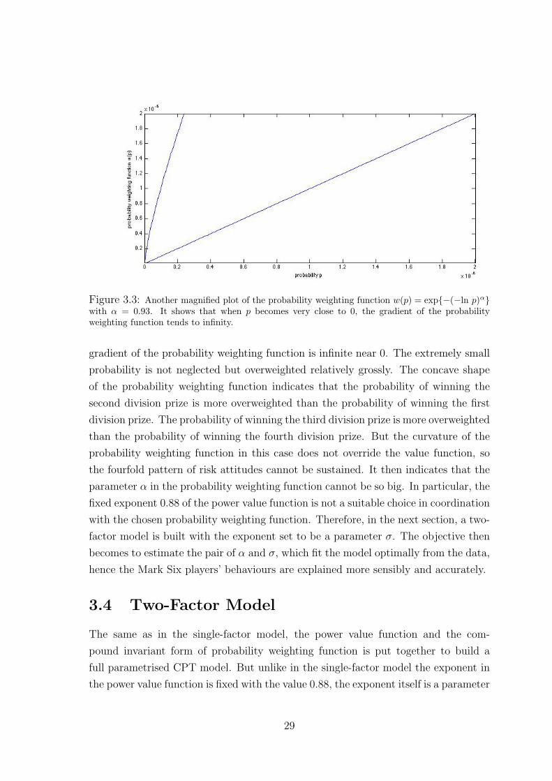
Figure 3.3: Another magnified plot of the probability weighting function w(p) = exp{−(−ln p)α}with α = 0.93. It shows that when p becomes very close to 0, the gradient of the probabilityweighting function tends to infinity.
gradient of the probability weighting function is infinite near 0. The extremely small
probability is not neglected but overweighted relatively grossly. The concave shape
of the probability weighting function indicates that the probability of winning the
second division prize is more overweighted than the probability of winning the first
division prize. The probability of winning the third division prize is more overweighted
than the probability of winning the fourth division prize. But the curvature of the
probability weighting function in this case does not override the value function, so
the fourfold pattern of risk attitudes cannot be sustained. It then indicates that the
parameter α in the probability weighting function cannot be so big. In particular, the
fixed exponent 0.88 of the power value function is not a suitable choice in coordination
with the chosen probability weighting function. Therefore, in the next section, a two-
factor model is built with the exponent set to be a parameter σ. The objective then
becomes to estimate the pair of α and σ, which fit the model optimally from the data,
hence the Mark Six players’ behaviours are explained more sensibly and accurately.
3.4 Two-Factor Model
The same as in the single-factor model, the power value function and the com-
pound invariant form of probability weighting function is put together to build a
full parametrised CPT model. But unlike in the single-factor model the exponent in
the power value function is fixed with the value 0.88, the exponent itself is a parameter
29

1st Division Prize 2nd Division Prize 3rd Division PrizeD0 HK$5638380 HK$667193 HK$39757D1 HK$6604683 HK$527847 HK$30588D2 HK$12588994 HK$735810 HK$38613D3 HK$18576056 HK$816305 HK$39061D4 HK$32402393 HK$786482 HK$41034D5 HK$36209011 HK$1041503 HK$42388D6 HK$26706946 HK$539056 HK$30977
Table 3.4: This table lists the averaged unit dividend of 1st, 2nd and 3rd division of the Mark Sixprize, with respect to the number of Jackpots before that draw. Note that the unit dividends for4th, 5th, 6th and 7th division are always fixed to be HK$4800, HK$320, HK$160, HK$20.
in two-factor model. Plus another parameter in the probability weighting function,
the nonlinearity on each dimension of the decision making problem is captured by one
parameter. The two-factor model of decision making under uncertainty is formulated
as
v(x) = xσ (3.4)
w(p) = exp{−(−ln p)α} (3.5)
Again, the lottery players are assumed to be indifferent between purchasing a
lottery ticket to enter Mark Six or not doing so. So the following relation holds
V (potential lottery prize) = V (lottery ticket price)
In order to find the parameters which fit the assumptions, model and data optimally,
the method of least squares estimation is employed for estimating the two parameters:
σ for money and α for probability.
3.4.1 Least Squares Estimation
It is started by collecting seven sets of unit dividend data, with respect to the number
of Jackpot before the lottery draw. Recall that the unit dividend of the fourth, fifth,
sixth and seventh division is fixed, but the unit dividend of the first, second and third
division is variable. So the unit dividend of the first, second and third division prize
of every single draw in the historical data are extracted, with respect to the number
of Jackpots before that draw. Then, the arithmetic average of unit dividends are
computed. D1, D2, . . . , D6 are vectors, whose elements are the unit dividends when
the number of Jackpots before that draw is ranging from 0 to 6. For example, D0 is
the vector consisting the unit dividends for the seven divisions of prize, when there is
30

ResidualD0 0.4634D1 0.4724D2 0.2328D3 0.0825D4 0.1652D5 0.2508D6 0.0114
Table 3.5: This table lists the residuals of each set of data, with σ = 0.42 and α = 0.70. Theresiduals are the difference between V (5) and V ((xi, pi)) for different sets of unit dividend data.
no Jackpot in the previous Mark Six draw, thereby it is the same payout data used
in the single-factor model discussed in previous chapter; D6 is the vector consisting
the unit dividends for the seven divisions of prize, when there are six Jackpots in the
previous draws. The values of Di are listed in Table 3.4.
Notice that the unit dividends are generally increasing as the number of Jackpot
is increasing. It is reasonable since the existence of Jackpot boosts the money in the
prize fund. However, the unit dividend of first division prize on the existence of six
Jackpots is less than the unit dividend on the existence of five Jackpots. An expla-
nation for this is that in the case there are six Jackpots, the amount of money in the
prize fund becomes enormous, the possible prizes become huge while the probabilities
of winning remain the same. Then it naturally attracts more people to enter the
lottery game, hence more people share the prizes. So the total prize is increasing and
the number of winning unit is also increasing, the unit dividend can become smaller.
Here each of the seven sets of unit dividend data cannot be expected to fit the
model perfectly. The best fit is obtained from the instance of the model for which
the sum of squared residuals has its least value.
f(σ, α) =6∑j=0
(V (5)− V ((xi, pi)))2
For each j, xi are substituted by the unit dividends in Dj. The objective of least
squares estimation here is to find a pair of (σ, α) which minimises the value of the
function f(σ, α). To estimate the optimal value of parameters, surface of the function
f is plotted in MATLAB initially with all possible values of σ ∈ (0, 1) and α ∈ (0, 1).
31

Figure 3.4: The surface plotted of the function f(σ, α) with parameter σ and α. It is found thatwhen σ = 0.42, α = 0.70, the value of function f(σ, α) reaches its minimum 0.57.
We identify the region where the value of f is smaller than elsewhere. Then the region
is refined and zoomed in to look for the values of σ and α more accurately.
3.4.2 Summary of Results
Figure 3.4 gives the plot for the surface of function f against two parameters σ and
α. The method of least squares estimation yields the parameter σ = 0.42 for the
power value function, and α = 0.70 for the compound invariant probability weighting
function. These two estimates give the minimum value of function f to be 0.57.
The residuals are calculated in order to analyse the accuracy of the estimation.
The residuals are the difference between V (5) and V ((xi, pi)) for different sets of lot-
tery data with the estimated parameters, hence the errors from our estimations. Table
3.5 lists all the residuals generated from the method of least squares estimation, with
respect to the seven sets of unit dividend data. All the residuals are close to each other
in value, and lie in the range from 0 to 0.5. The squared residuals can be even smaller.
However, let us consider the factors that data obtained only covers seven years of
lottery sales; the unit dividends used in calibration, are the arithmetic averages from
each draw; and the accurate level we can get with current computing capability. The
result of estimation is acceptable and sufficient as evidences for examining people’s
behaviours of making decisions under uncertainty. As a comparison, pick up a pair
32

ResidualD0 29.64D1 30.98D2 44.32D3 54.59D4 73.55D5 79.04D6 64.82
Table 3.6: This table lists the residuals of each set of data, with the parameters estimated by Prelec.The residuals are the difference between V (5) and V ((xi, pi)) for different sets of unit dividend data.
of estimation of σ and α in the literature, σ = 0.60 and α = 0.65 were estimated
with the same model by Prelec [12], from his questionnaires among 39 MIT students.
Table 3.6 shows the residuals with Prelec’s estimations. It is obvious that Prelec’s
estimation from artificial experiment does not fit the present data. Hence, it shows
the advantages of using real-life data to calibrate the model. Note that the differences
between our estimation and Prelec’s are only 0.18 for σ and 0.05 for α, but they lead
to the differences of scale 104 in the value of V ((xi, pi)).
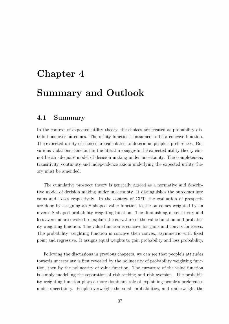
Figure 3.5 shows the plot of power value function with σ = 0.42. It is clear that
the value function is concave in the positive domain, in accord with the principle
of diminishing sensitivity. Figure 3.6 is the plot of probability weighting function
with α = 0.70, in the full range of probability from 0 to 1. This plot exhibits that
the probability weighting function is inverse S shaped; it is concave then convex,
the convex region is about twice bigger than the concave region; it is asymmetric
and regressive. Figure 3.7 is the same plot but for the extremely small interval
near zero. It zooms in for the range of values between 0 to 8 × 10⁻⁸ in order to
achieve a better resolution for small probabilities. It can be seen that the probability
weighting function declines to zero smoothly; the extremely small probabilities are
overweighted significantly; the difference between two extremely small probabilities
become relatively indistinguishable; the gradient of the probability weighting function
tends to infinity near zero. Hence it reflects the fourfold pattern of risk attitudes, as
discussed in Section 2.3. They also indicate that our assumption about the lottery
players are indifferent in entering the lottery game or not, is correct. Overall, it
appears that the CPT model can provide a reasonably good description for lottery
players’ behaviours when making decisions under uncertainty.
33
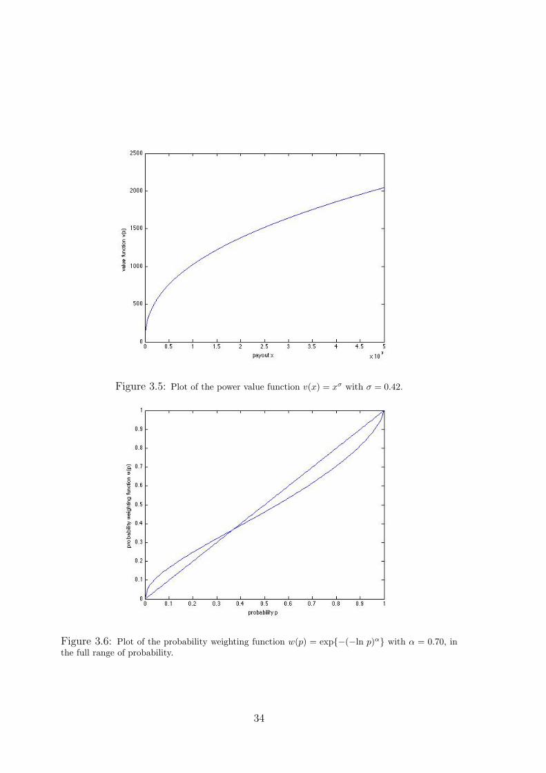
Figure 3.5: Plot of the power value function v(x) = xσ with σ = 0.42.
Figure 3.6: Plot of the probability weighting function w(p) = exp{−(−ln p)α} with α = 0.70, inthe full range of probability.
34

Figure 3.7: Plot of the probability weighting function w(p) = exp{−(−ln p)α} with α = 0.70, foran extremely small interval of probability near zero.
35

36
Chapter 4
Summary and Outlook
4.1 Summary
In the context of expected utility theory, the choices are treated as probability dis-
tributions over outcomes. The utility function is assumed to be a concave function.
The expected utility of choices are calculated to determine people’s preferences. But
various violations came out in the literature suggests the expected utility theory can-
not be an adequate model of decision making under uncertainty. The completeness,
transitivity, continuity and independence axiom underlying the expected utility the-
ory must be amended.
The cumulative prospect theory is generally agreed as a normative and descrip-
tive model of decision making under uncertainty. It distinguishes the outcomes into
gains and losses respectively. In the context of CPT, the evaluation of prospects
are done by assigning an S shaped value function to the outcomes weighted by an
inverse S shaped probability weighting function. The diminishing of sensitivity and
loss aversion are invoked to explain the curvature of the value function and probabil-
ity weighting function. The value function is concave for gains and convex for losses.
The probability weighting function is concave then convex, asymmetric with fixed
point and regressive. It assigns equal weights to gain probability and loss probability.
Following the discussions in previous chapters, we can see that people’s attitudes
towards uncertainty is first revealed by the nolinearity of probability weighting func-
tion, then by the nolinearity of value function. The curvature of the value function
is simply modelling the separation of risk seeking and risk aversion. The probabil-
ity weighting function plays a more dominant role of explaining people’s preferences
under uncertainty. People overweight the small probabilities, and underweight the
37

moderate or high probabilities. They are risk seeking to small probabilities of gains
and large probabilities of losses; risk averse to small probabilities of losses and large
probabilities of gains. The risk seeking and risk aversion are further enhanced by the
shape of value function.
Prelec’s theory claims the probability weighting function must satisfy the com-
pound invariance and the diagonal concavity condition. Then the compound invariant
form of probability weighting function is proposed in order to unify the characteris-
tics of probability weighting function. It has been shown in our experiments that the
characteristics of Mark Six lottery players’ attitudes towards uncertainty can be cap-
tured in the CPT model by combining the power value function and the compound
invariant form of probability weighting function.
4.2 Outlook
A feature may need to be added to the model more explicitly is the source depen-
dence. People’s desirability to an outcome not only depends on how uncertain the
outcome is but also depends on the where the uncertainty is generated from. Natu-
rally if the uncertainty comes from somewhere within a decision maker’s competence,
it can lead the decision maker to be more risk seeking towards this uncertainty. Heath
and Tversky [6] found that when a sports fan has to choose whether to bet on sport
games for 50% chance of winning or a fair coin toss game. He will actually prefer
betting on the sports game. People are generally trying to avoid the uncertainty
from ambiguous prospects. To reflect this effect, we may consider to call different
probability weighting function in different domains.
Also as mentioned before, when making decision under uncertainty, people simplify
the choice to whatever representations better for them to evaluate. Different framing
of the choices can lead to totally different evaluation of the prospects. The current
theory of decision making only focuses on the evaluation procedure. It is rather an
incomplete theory. So far, there is no unified method for modelling the framing phase
and evaluation phase jointly.
38

References
[1] Arrow, J., 1951, “Alternative Approaches to the Theory of Choice in Risk-Taking
Situations”, Econometrica, 19, pp. 404-437
[2] Allais, M., 1953, “ Le comportement de lhomme rationnel devant le risque: cri-
tique des postulats et axiomes de I’ecole Americain”, Econometrica, 21, pp.
503-546
[3] Bernoulli, D., 1954, “Exposition of a New Theory on the Measurement of Risk”
(original: 1738), Econometrica, 22, pp. 23-36
[4] Cramer, G., 1728, “Letter to Nicolas Bernoulli, a cousin of Daniel Bernoulli”,
see Bernoulli 1954
[5] Fishburn, C and Kochenberger, A., 1979, “Two-piece von Neumann-Morgenstern
Utility Functions”, Decision Science, 10, pp. 503-518
[6] Heath, C and Tversky, A., 1991, “Preference and Belief: Ambiguity and Com-
petence in Choice under Uncertainty”, Journal of Risk and Uncertainty, 4, pp.
5-28
[7] Kahneman, D. and Tversky, A., 1979, “Prospect theory: An Analysis of Decision
under Risk”, Econometrica, 47, pp. 263-291
[8] Markowitz, H., 1952, “The Utility of Wealth”, Journal of Political Economy, 60,
pp. 151-158
[9] MacCrimmon, K. and Larsson S., 1979, “Utility Theory: Axioms Versus ‘Para-
doxes”, in Allais M. and Hagen O. 1979, Expected utility and the Allais paradox,
Reidel, Dordrecht, pp. 333-409
[10] Neumann, J. and Morgenstern, O., 1944, Theory of Games and Economic Be-
havior, Princeton, NJ, Princeton University Press
39

[11] Prelec, D., 1998, “The Probability Weighting Function”, Econometrica, 66, pp.
497-527
[12] Prelec, D., 2008, ”Compound Invariant Weighting Functions in Prospect The-
ory”, Choices, Values and Frames, ed. Kahneman, D. and Tversky, A., 8th print-
ing, Cambridge, Cambridge University Press, pp. 86-88
[13] Quiggin, J., 1982, “A theory of Anticipated Utility”, Journal of Economic Be-
haviour and Orgnization, 3, pp. 323-343
[14] Tversky, A. and Kahneman, D., 1986, “Rational Choice and the Framing of
Decisions”, The Journal of Business, 59, part 2, pp. 251-278
[15] Tversky, A. and Kahneman, D., 1991, “Loss Aversion in Riskless Choice: a
Reference Dependent Model”, Quarterly Journal of Economics, 107, pp. 1039-
1061
[16] Tversky, A. and Kahneman, D., 1992, “Advances in Prospect Theory: Cumu-
lative Representation of Uncertainty”, Journal of Risk and Uncertainty, 5, pp.
297-323
[17] Weber, M. and Camerer, C., 1987, “Recent Developments in Modelling Prefer-
ences Under Risk”, OR Spektrum, 9, pp. 129-151
[18] Wakker, P., 1990, “Under Stochastic Dominance Choquet-Expected Utility and
Anticipated Utility are Identical”, Theory and Decision, 29, pp. 119-132
[19] Wakker, P. and Tversky, A., 1993, “An Axiomatization of Cumulative Prospect
Theory”, Journal of Risk and Uncertaity, 7, pp. 147-176
[20] Wakker, P., 1994, “Separating Marginal Utility and Probabilistic Risk Aversion”,
Theory and Decision, 36, pp. 1-44
[21] The Official Web Site of the Hong Kong Jockey Club, http://www.hkjc.com/
english/index.asp, (accessed 9 May 2008)
[22] The Official Web Site of the Nobel Foundation, “The Sveriges Riksbank Prize
in Economic Sciences in Memory of Alfred Nobel 2002”, http://nobelprize.
org/nobel_prizes/economics/laureates/2002/, (accessed 9 May 2008)
40