BEHAVIORAL FINANCE: LEARNING FROM MARKET … · BEHAVIORAL FINANCE: LEARNING FROM MARKET ANOMALIES AND PSYCHOLOGICAL FACTORS Natalia del Águila* Abstract: Empirical research has

BEHAVIORAL FINANCE: LEARNING FROM MARKETANOMALIES AND PSYCHOLOGICAL FACTORS

Natalia del Águila*

Abstract: Empirical research has shown that, when selecting a portfolio,

investors not only consider statistical measures such as risk and return, but

also psychological factors such as sentiment, overconfidence and overreaction.

In short, heuristic-driven bias, frame dependence, and market inefficiency

shape the kind of portfolios that investors chose, the type of securities investors

find attractive, and the biases to which investors are subject. As a consequence,

the purpose of the paper is to identify those psychological factors that play

an important role in their decisions. Specifically, the paper reviews the

existing literature on overconfidence and overreaction, defining the factors,

analyzing their implications, identifying questions that have been left

unanswered, and addressing the implication of these factors on market

efficiency and investors’ rational behavior. Finally, and in trying to contribute

to the theory of Behavioral Finance, some future steps and research are

proposed.

Introduction

Traditional Portfolio Theory believes in efficient markets, which means that

the prices of the securities coincide with their fundamental value. As maintained

by the efficient market school, investors are rational; i.e. their investment

decisions are made according to their risk aversion, which is measured by

the mean and variance of the returns. One of the pillars of standard finance

* Master en Finanzas (Universidad Torcuato Di Tella), Master in Human Resources Management(Washington University in St. Louis). Investigadora del Centro de Entrepreneurship yDesarrollo de Negocios (Universidad Torcuato Di Tella). [email protected]

Revista de Instituciones, Ideas y Mercados Nº 50 | Mayo 2009 | pp. 47-104 | ISSN 1852-5970

was developed by Harry Markowitz, who developed the theory of mean-

variance portfolios, offering a frontier of efficient portfolios with different

risk-return combinations from where investors can choose given their risk

aversion.

However, the major factors driving portfolio selection are much more

complex than the mean and variance of future returns and the efficient frontier.

Over the last 25 years, scholars began to discover empirical results that were

not consistent with the view that market returns were determined in accordance

with the efficient market theory. Additionally, empirical research shows that,

when selecting a portfolio, portfolio managers not only consider statistical

measures such as risk and return, but also psychological factors such as

sentiment, overconfidence, overreaction, etc. As these factors begun to be

identified by scholars, a new school of thought began to emerge; that of

Behavioral Finance.

Behavioral Finance (BF) is the application of psychology to financial

behavior; i.e. it is the behavior of practitioners. According to BF, investors

are rational, but not in the linear and mathematical sense based on the mean

and variance of returns. Instead, investors respond to natural psychological

factors such as fear, hope, optimism and pessimism. As a result, asset values

may deviate from their fundamental value and the theory of market efficiency

suffers.

Empirical research has shown that these behavioral factors do exist and

that they are, in fact, considered by the market. Thus, this may imply that

the market goes beyond the traditional theory of finance. In short, heuristic-

driven bias, frame dependence, and market inefficiency shape the kind of

portfolios that investors chose, the type of securities investors find attractive,

and the biases to which investors are subject.

As a result, the purpose of the present paper is to identify not only the

statistical measures that influence investors’ decision making, but also the

psychological factors that play an important role in their decisions.

Specifically, the paper will review the existing literature on two of the

main behavioral factors that affect portfolio selection, analyzing if the

factor and its implications have correctly been defined, and identifying

48 | RIIM Nº50, Mayo 2009

questions that have been left unanswered. In particular, the paper will

address overconfidence and overreaction and their implication on market

efficiency and investors’ rational behavior. Finally, some future steps will

be proposed.

The structure of the paper is as follows: Section I explains briefly the

assumptions underlying Traditional Portfolio Theory; Section II concentrates

on Behavioral Finance and its beginnings; Section III reviews the literature

on overreaction and overconfidence, concentrating mainly on empirical

research; Section IV discusses the implications for market efficiency and

investors’ rational behavior as well as the responses given by the Traditional

Finance Theory, and Section V proposes some future steps for research.

I. Traditional Portfolio Theory

The beginning of Standard Finance is generally considered to be the publication

of “Portfolio Selection” by Harry Markowitz in 1952, who described how

rational investors should create portfolios given a set of return expectations,

volatilities and cross correlations. A rational investor maximizes expected

returns and minimizes risk. The investor is pressured by two opposing forces:

the desire to make earnings and the dissatisfaction produced by risk. In this

way, risk and return are the two key features of investment strategy, where

risk is measured as the average (or mean) absolute deviation and the standard

deviation (Sharpe, 1985).

In order to select portfolios, the model requires the following information:

(1) expected returns of the assets; (2) standard deviation of each asset; and

(3) covariance between the returns of every pair of assets. Given this

information, it is possible to construct an efficient portfolio frontier.

A portfolio is efficient when it offers the highest return given a specific

risk, or the minimum risk given a specific return. Consequently, the group

of efficient portfolios can be determined by solving one of the following

two problems:

RIIM Nº50, Mayo 2009 | 49

a. Maximize expected return of the portfolio for a given portfolio risk:

E[Rp] = X1 E[R1] + X2 E[R2] + … + Xn E[Rn]

Subject to: σ2p = ΣiΣj Xi Xj σij = V*

X1 + X2 + … + Xn = 1

X1, X2, …, Xn ≥ 0

b. Minimize portfolio risk for a given portfolio expected return:

σ2p = ΣiΣj Xi Xj σij

Subject to: E[Rp] = X1 E[R1] + X2 E[R2] + … + Xn E[Rn] = Rp*

X1 + X2 + … + Xn = 1

X1, X2, …, Xn ≥ 0

The portfolios on the frontier are efficient in the sense that they offer the

highest E[Rp] for each value of σp, or the lowest σp for each value of E[Rp].

But in order to determine the “optimal” portfolio for the investor, it is

necessary to understand the investor’s utility function, expressed as indifference

curves. The rational investor will choose assets that offer high expected

returns and low risk (it is assumed that all investors are risk averse). As a

result, the investor’s utility function (μ) is defined as follows:

μ = F (E[Rp], σ2p)

∂ μ / ∂ E[Rp] > 0

∂ μ / ∂ σ2p < 0

Finally, the tangent point between the investor’s indifference curves and

the efficient frontier, will determine the desired risk-return combination.

Once this portfolio is selected, it is possible to obtain the percentages to

invest in each of the assets that form the portfolio (Xi).

Markowitz’s main contribution was suggesting that the stock’s risk should

be evaluated not in isolation, but also in terms of its contribution to the risk

of a diversified portfolio. He showed how an investor can reduce portfolio


risk by choosing stocks that do not move together; i.e. that they are not

affected by the same factors. In statistical terms, this means that stock prices

are not perfectly correlated and risk can be eliminated through diversification.

Sharpe (1964) extended the original work of Markowitz and developed

the Capital Asset Pricing Model (CAPM). Sharpe incorporated the Markowitz

mean-variance-optimizer investor as well as the concept of efficient markets.

The CAPM assumes that individuals are identical in expectations, investment

horizon and access to available securities. Additionally, it assumes that

individuals can borrow and lend at the same interest rate, the risk-free rate

(Rf). As a result, some combination of Rf and the tangency efficient portfolio

will offer a better risk/reward trade-off, at every level of risk, than other

points on the Markowitz efficient frontier. Since there is only one risky

portfolio that is held by all rational investors, that portfolio must be the

market (Fabozzi, 1998).

This theory is also based on the assumption that markets do not compensate

investors for assuming risk that can be reduced or eliminated through

diversification. Total risk is considered to be the sum of systematic and

unsystematic risk. Systematic risk, measured by beta, captures the reaction

of different individual securities or portfolios to changes in the market

portfolio. This risk cannot be eliminated through diversification because

securities’ prices tend to move, to a certain extent, with the market (there

are several macroeconomic variables that affect, to a more or lesser extent,

all industries and, consequently, stocks tend to move in the same direction).

On the other hand, unsystematic risk reflects the variability in the prices

of the securities due to factors which are internal to the firm or to the industry

in which the firm operates. As a result, as the CAPM sustains that investors

will receive higher returns only if they assume higher systematic risk, and

as beta is the indicator of systematic risk, the return of the securities is a

linear function of beta (Gonzalez Isla, 2006).1

To sum up, the main implications of the CAPM are that (1) the market

portfolio is mean-variance efficient; and (2) the average return is an increasing

function of beta.


Efficient Market Hypothesis

Traditional Finance assumes market efficiency. Although Fama officially

introduced the notion of an “efficient” market in 1965, the empirical research

that preceded the efficient market hypothesis modeled price behavior in

statistical terms, and it received the name of “random walk hypothesis”.

Under the assumptions of this hypothesis, successive daily stock price changes

were independent; i.e. they displayed no discernable trends or patterns that

could be exploited by investors (Ball, as cited in Chew 1999). In other words,

random walk means that no prediction of the future movements can be made

based on historic information.

Fama (1965) defined an efficient market as one ‘where there are large

numbers of rational, profit-maximizers actively competing with each other,

trying to predict future market values of individual securities, and where

important current information is almost freely available to all participants’.

As a result, a market is efficient with respect to an information set if it is

impossible to earn consistent abnormal profits by trading on the basis of the

information set (Daniel, 2002).

Three types of market efficiency have been identified:

Weak: market efficiency in its weak form means that no investor can earn

consistent abnormal profits trading on the basis of past- price information;

that prices reflect all the information contained in historic prices. Some

implications of weak form efficiency are that technical analysis is not profitable

as there is no price momentum or price reversal.

Semi-strong: market efficiency in this form means that no investor can

earn consistent abnormal profits trading on any public information; i.e.

that prices not only reflect historic prices, but also any additional public

information (such as earnings announcements, dividends, etc). Implications

of semi-strong form efficiency are that fundamental analysis and trading

based on the published earnings forecasts or analysts’ reports are not

profitable.

Strong: market efficiency in its strong form means that no investor can

earn consistent abnormal profits trading on the basis of any information,


private or public. An implication of strong form efficiency is that insider

trading is not profitable.

In an efficient market, the changes in prices are random, because if prices

always reflect all the relevant information, they will only change under new

information (by definition, new information cannot be anticipated).

Consequently, changes in prices cannot be predicted. In other words, if prices

already reflect everything that is “predicted”, then changes in prices must

only reflect the “unpredictable”. In a perfectly efficient market, prices will

always equal fair values.

In regards to the accomplishment and limitations in the theory of Efficient

Markets and Rational Investors, a large body of empirical research in the

70’s provided evidence of market efficiency that offered strong support for

the CAPM and the models that followed, such as the Arbitrage Pricing Theory

and Option Pricing models. However, and in spite of all its accomplishments,

the efficient markets theory also had its setbacks. After a period in which

one triumph of modern financial theory succeeded another, research began

to accumulate evidence of “anomalies” that appeared to contradict the theory

of efficient markets (Chew, 1999).

Additionally, the theory of rational behavior also began to suffer. Most

recent literature identified under the concept of Behavioral Finance, shows

that investors behave in a non-rational way. Jensen (as cited in Chew,

1999) describes non-rational behavior as the behavior that ‘arises under

conditions of fear’. While attempting to avoid the pain associated with

acknowledgments of their mistakes, people often end up incurring more

pain and making themselves worse off. Jensen believes that this non-

rational behavior is not random. LeDoux (1994) suggests that such

counterproductive defensive responses derive from the biological and

chemical structure of the brain, and are connected to the brain’s “fight or

flight” response. The mechanisms of the brain commonly blind people so

that they are unaware of their own fear and defensiveness. And the primary

consequence of such defensiveness is the reluctance of people to learn

and their resulting inability to respond properly to feedback and change

(Jensen, as cited in Chew 1999).


Finally, investors recognize that due to the inefficiency present in financial

markets, prices may not be correctly reflecting all the information available;

i.e. some securities may be over or undervalued. It is the portfolio manager’s

job to identify these opportunities and adopt an investment strategy accordingly.

II. Behavioral Finance

Behavioral finance (BF) is the application of psychology to financial behavior,

the behavior of practitioners. Even though the idea that psychology plays

an important role in investors’ behavior became popular only recently, several

economists and psychologists have been trying to integrate these fields for

quite some time.

Keynes wrote of the influence of psychology in economics more than

fifty years ago. Additionally, psychology Professor Paul Slovic published a

detailed study of the investment process from a behavioral point of view in

1969. However, it was not until the late 1980s that BF began to get acceptance

among professional economists. At that time, Professors Richard Thaler at

the University of Chicago, Robert Shiller at Yale University, Werner de Bondt

at the University of Illinois, and Meir Statman and Hersh Shefrin at Santa

Clara University, among others, began to publish research relevant to

Behavioral Finance (Olsen, 1998).

These scholars began to discover a host of empirical results that were

not consistent with the view that market returns were determined in

accordance with the CAPM and the efficient market hypothesis. Proponents

of Traditional Finance regarded these findings as anomalous, and thus

called them anomalies. BF’s main contribution was to allow a better

understanding of the anomalies present in investors’ behavior by integrating

psychology with finance and economics. However, it was not until Professor

Daniel Kahneman of Princeton University was awarded the 2002 Nobel

Prize in economic sciences that BF gained momentum.2 Consequently, it

was not until researchers began to discover empirical results that were not

consistent with the efficient market theory that BF became popular. In


short, the growing interest in BF has been the result of an accumulation

of empirical anomalies.

Shefrin (1998) categorizes the behavioral factors identified throughout

the years into three broad themes:

Heuristic-driven bias: The dictionary definition for the word heuristic

refers to the process by which people find things out for themselves, usually

by trial and error. Trial and error often leads people to develop rules of thumb,

but this process often leads to other errors. As a result, BF believes that

practitioners commit errors because they rely on rules of thumb; BF recognizes

that practitioners use rules of thumb called heuristics to process data. One

example of rules of thumb is: ‘past performance is the best predictor of future

performance, so invest in a mutual fund having the best five-year record’.

But rules of thumb are generally imperfect. Therefore, practitioners hold

biased beliefs that predispose them to commit errors. In contrast, Traditional

Finance assumes that when processing data, practitioners use statistical tools

appropriately and correctly.

Frame dependence: BF postulates that in addition to objective

considerations, practitioners’ perception of risk and return are highly influenced

by how decision problems are framed. In contrast, Traditional Finance

assumes frame independence, meaning that practitioners view all decisions

through the transparent, objective lens of risk and return.

Inefficient markets: BF assumes that heuristic-driven bias and framing

effects cause market prices to deviate from fundamental values. In contrast,

Traditional Finance assumes that markets are efficient, meaning that the

price of each security coincides with fundamental value.

However, it is important to highlight that only the first two themes -

heuristic-driven bias and frame dependence- are form of biases, while the

theme regarding inefficient markets is a result of bias.

As Shefrin (1998) also summarizes, the main empirical anomalies that

affect investors’ behavior and their financial decisions, and that have also

led to a reevaluation of the efficient markets hypothesis, are:

Anchoring and adjustment (conservatism): Analysts who suffer from

conservatism due to anchoring and adjustment do not adjust their earnings


predictions sufficiently in response to the new information contained in

earnings announcements. Therefore, they find themselves surprised by

subsequent earnings announcements.

Aversion to ambiguity: People prefer the familiar to the unfamiliar. The

emotional aspect of aversion to ambiguity is fear of the unknown.

Disposition effect: According to the disposition effect, investors have

great difficulty coming to terms with losses. Consequently, they are predisposed

to holding losers too long and selling winners too early.

Emotional time line: It is important to discuss emotion while analyzing

financial decisions because emotions determine tolerance for risk. According

to psychologist Lopes (1987), hope and fear affect the way that investors

evaluate alternatives. Lopes tells us that these two emotions reside within

all of us, as opposite poles, and one of her contributions is to establish how

the interaction of these conflicting emotions determines the tolerance towards

risk.

Loss aversion and “get-evenitis”: Kahneman and Tversky (1979) studied

how people respond to the prospect of loss. They find that a loss has about

two and a half times the impact of a gain of the same magnitude and they

call this phenomenon loss aversion (Prospect Theory).

Momentum: Momentum takes places when stocks that get recommended

are those that have recently done well.

Overconfidence: When people are overconfident, they set overly narrow

confidence bands. They set their high guess too low and their low guess too

high. There are two main implications of investor overconfidence. The first

is that investors take bad bets because they fail to realize that they are at an

informal disadvantage. The second is that they trade more frequently than

is prudent, which leads to excessive trading volume. Additionally, this

behavioral factor can be related to another empirical anomaly: Betting on

Trends. De Bondt (1993) reports that people tend to formulate their predictions

by naively projecting trends that they perceive in the charts. Second, they

tend to be overconfident in their ability to predict them accurately. Third,

their confidence intervals are skewed, meaning that their best guesses do

not lie midway between their low and high guesses.


Port-recommendation drift: When an analyst changes a recommendation,

the market price immediately reacts to the announcement, but the adjustment

continues for a substantial period thereafter, affecting market efficiency

(market efficiency holds that prices adjust virtually immediately to new

information; post-recommendation drift is not a property of efficient prices).

Regret: Regret is the emotion experienced for not having made the right

decision. Regret is more than the pain of loss. It is the pain associated with feeling

responsible for the loss. People tend to experience losses even more acutely

when they feel responsible for the decision that led to the loss. Regret can affect

the decisions people make, as they try to minimize possible future regret.

Representativeness and overreaction: This principle refers to judgments

based on stereotypes. A financial example illustrating representativeness is

the winner-loser effect documented by De Bondt and Thaler (1985, 1987).

Investors who rely on the representativeness heuristic become overly

pessimistic about past losers and overly optimistic about past winners. As a

consequence, investors overreact to both bad and good news. Therefore,

overreaction leads past losers to become underpriced and past winners to

become overpriced.

Sentiment: Sentiment is the reflection of heuristic-driven bias.

Separate mental accounts: This occurs when two decision problems

together constitute a concurrent package but the investor does not see the

package; instead the choices are separated into mental accounts.

III. Main behavioral factors that affect financial decisions:overreaction and overconfidence

As mentioned in the previous section, empirical research has shown that the

behavioral factors do exist and that they are, in fact, considered by the market.

As a result, the purpose of this section is to review the psychological factors

that play an important role in investors’ decisions. In order to focus the study,

De Bondt (1998) has been used to narrow the selection of empirical anomalies

to two factors: overconfidence and overreaction. De Bondt identified and


reviewed four classes of anomalies regarding individual investors that have

to do with: (1) investors’ perceptions of the stochastic process of asset prices;

(2) investors’ perceptions of value; (3) the management of risk and return;

and (4) trading practices.

De Bondt illustrated these anomalies with selected results from a study

of 45 individual investors in the Fox Valley in Wisconsin (USA). The investors

were recruited at a conference organized by the National Association of

Investment Clubs in Appleton. Every investor personally managed an equity

portfolio and the mean value of their financial portfolio was $310,000

(excluding real estate). The investors also agreed to make repeated weekly

forecasts of the Dow Jones Industrial Average (DJIA) and of the share prices

of one of their main equity holdings; i.e. the study tracked the group’s forecasts

for the future performance of both the Dow Jones and their own stocks. The

research took place between October 1994 and March 1995.

De Bondt’s findings showed the following:

(i) Investors were excessively optimistic about future performance of the

shares they owned but not about the performance of the DJIA.

(ii) They were overconfident in that they set overly narrow confidence

intervals relative to the actual variability in prices. They set their high

guess too low and their low guess too high. Additionally, the confidence

intervals were asymmetric. The average investor imagined more

downward than upward return variability. As a result, they found

themselves surprised by price changes to their stocks more frequently

than they had anticipated.

(iii) Their stock price forecasts were anchored on past performance.

(iv) They rejected the notion of risk that relied on whether the price of a

stock moved with or against the market (they underestimated the

covariance in returns between their portfolios holdings and the market

index; i.e. they underestimated beta). Additionally, they discounted

diversification; i.e. holding few stocks was a better risk management

tool than diversification

In short, De Bondt’s survey highlights two of the most important behavioral

factors that have been affecting financial decisions over the years: overconfidence


and overreaction. Specifically, the survey informs us that individual investors

display excessive optimism and overconfidence, and that they overreact to

both bad and good news. These anomalies can widely be seen among investors’

behavior and their impact on financial decisions is very strong. As a

consequence, these anomalies constitute two of the main areas of interest

that BF scholars have nowadays.

Consequently, this section focuses on the anomalies on overconfidence

and overreaction, trying to (1) identify their main issues and propositions;

(2) review the empirical models that were used; and (3) develop a strength

and weakness analysis, discussing if the research designs were appropriate

to measure the behavioral factor and if questions have been left unanswered.

Overconfidence

1) Identification of its main issues and propositions.

Psychological studies have found that people tend to overestimate the precision

of their knowledge (Lichtenstein, Fischhoff and Philips, 1982), and this can

be found in many professional fields. They also found that people overestimate

their ability to do well on tasks and these overestimates increase with the

personal importance of the task (Frank, 1935). People are also unrealistically

optimistic about future events; they expect good things to happen to them

more often than to their peers (Weinstein, 1980 and Kunda, 1987). Additionally,

most people see themselves as better than the average person and most

individuals see themselves better than others see them (Taylor and Brown,

1988).

In regards to financial markets, when people are overconfident, they set

overly narrow confidence bands. They set their high guess too low and their

low guess too high. There are two main implications of investor overconfidence.

The first is that investors take bad bets because they fail to realize that they

are at an informal disadvantage. The second is that they trade more frequently

than is prudent, which leads to excessive trading volume (Shefrin, 1998). As

a result, financial markets are affected by overconfidence. But how are markets

affected by this overconfidence factor?


2) Empirical models: research designs and methodology.

Several finance researchers have focused their research on overconfidence;

perhaps the work by Terence Odean can be considered as more explanatory.3

For Odean (1998) overconfidence is a characteristic of people, not of markets,

and some measures of the market, such as trading volume, are affected

similarly by the overconfidence of different market participants. However,

other measures, such as market efficiency, are affected in different ways but

different market participants. One of the most important factors that determine

how financial markets are affected by overconfidence is how information

is distributed in a market and who is overconfident.

Odean (1998) examined how markets were affected by studying

overconfidence in three types of traders: (i) price-taking traders in markets

where information was broadly disseminated; (ii) strategic-trading insider

in markets with concentrated information; and (iii) risk-averse market makers.

In particular, he analyzed market models in which investors were rational

in all aspects except in how they valued information. Additionally, the paper

differed from related work on overconfidence in the sense that it examined

how the effects of overconfidence depended on who in a market was

overconfident and on how information in that market was disseminated.

The main assumptions of the empirical models were:

a. Overconfidence was modeled as a belief that a trader’s information was

more precise than it actually was.

b. How heavily information is weighted depended not only on overconfidence

but also on the nature of the information. Psychologists find that when

making judgments and decisions, people overweight salient information

(Kahneman and Tversky (1973), Grether (1980). As a result, people are

prone to gather information that supports their beliefs, and readily dismiss

information that does not (Lord, Ross and Lepper (1979), Nisbett and

Ross (1980), Fiske and Taylor (1991). In short, the overconfidence

literature indicates that people believe their knowledge is more precise

than it really is, they rate their own abilities too highly when compared

to others, and they are excessively optimistic.

c. In the models, traders updated their beliefs about the terminal value of


a risky asset on the basis of three sources of information: a private signal,

their inferences from market price regarding the signals of others, and

common prior beliefs. Consequently, and in consistence with the

overconfidence literature, traders overweighed their private signals, they

overweighed their own information relative to that of others, and they

overestimated their expected utility.

d. The main difference between the insider model and the price-takers model

is that the insider model has noise traders and information is distributed

in a different way. In the price-takers model, all traders received a signal,

while in this model information is concentrated in the hands of a single

insider. It is a one-period model in which a risk-neutral, privately informed

trader (the insider) and irrational noise traders submit market orders to

a risk neutral market maker.

e. The market-makers model differs from the previous two models in the

sense that the participants in this trading are the traders who buy the

information (informed traders), traders who do not buy the information

(uninformed traders) and noise traders who buy or sell without regard

to price or value. Risk-averse traders decide whether or not to pay for

costly information about the terminal value of the risky asset; those who

buy information receive a common signal and a single round of trading

takes place. All traders, even those who remain uninformed, are

overconfident about the signal. In the previous models, traders were

overconfident about their own signals but not those of others. Here,

everyone believes the information is better than it is, but some decide

the cost is still too high.

Odean then tested the following hypothesis in the three models:

Proposition 1: Does expected trading volume increase as overconfidence

increases?

Proposition 2: Does overconfidence affect market efficiency?

Proposition 3: Does volatility of prices increase as overconfidence increases?

Proposition 4: Does overconfidence affect expected utility?

The results of Odean’s study can be summarized as follows:

The effects of overconfidence were studied in three market settings that


differed mainly on how information was distributed and on how prices were

determined. For some market measures, such as trading volume,

overconfidence had a similar effect in each setting; i.e. overconfidence in

the three types of traders increased expected trading volume. As a consequence,

overconfidence increased market depth. When an insider was overconfident,

he traded more aggressively for any given signal. The market maker adjusted

for this additional trading by increasing market depth.

For other measures, such as market efficiency, the effect of overconfidence

was not so clear. Whether overconfidence improves or worsens market

efficiency depends on how information is distributed in the market. For

example, when information was distributed in small amounts to many traders

or when it was publicly disclosed and then interpreted differently by many

traders, overconfidence caused the aggregate signal to be overweighed. This

led to prices further from the asset’s true value than would otherwise be the

case. Though all information was revealed in such a market, it was not

optimally incorporated into price. On the other hand, when information was

held exclusively by an insider and then inferred by a market maker from

order flow, overconfidence prompted the insider to reveal, through aggressive

trading, more of his private information than he would otherwise would

have, and therefore enabled the market maker to set prices closer to the

asset’s true value. Price-taking traders, who were overconfident about their

ability to interpret publicly disclosed information, reduced market efficiency;

overconfident insiders temporarily increased it. Nonetheless, overconfidence

affected market efficiency.

In regards to volatility, traders’ overconfidence increased volatility while

market makers’ overconfidence may have lowered it. However, in a market

with many traders and few market makers it is unlikely that the decrease in

volatility by overconfident market makers will offset increases in volatility

due to overconfident trader.4 Overconfidence reduced the expected utility

of overconfident traders, who did not properly optimize their expected

utilities, which were therefore lower than if the traders were rational.

Finally, the impact of a private signal depends on how many people

received that signal. The impact of traders, even rational traders, depended


on their numbers and on their willingness to trade. The mere presence of a

few rational traders in a market did not guarantee that prices were efficient;

rational traders may have been no more willing or able to act on their beliefs

than biased traders. However, it was markets with higher proportions of

rational traders that would be more efficient.

But how can these models be applied in practice? Odean believed that

how each model is used depends on the characteristics of the market. For

example, for a market in which crucial information is first obtained by well-

capitalized insiders and market makers are primarily concerned about trading

against informed traders, then the model of the overconfident insider is

appropriate. However, if relevant information is usually publicly disclosed

and then interpreted differently by a large number of traders each of whom

has little market impact, the overconfident price-taker model applies. Finally,

the market maker model would apply to markets in which traders choose

between investing passively and expending resources on information and

other costs of active trading.

Barber and Odean (1999) also believe that high levels of trading in

financial markets are due to overconfidence. They sustain that overconfidence

increases trading activity because it causes investors to be too certain about

their own opinions and to not consider sufficiently the opinion of others.

Overconfident investors also perceive their actions to be less risky than

generally proves to be the case. In their paper, they test whether a particular

class of investors, those with accounts at discount brokerages, trade excessively,

in the sense that their trading profits are insufficient to cover their trading

costs.

To test for overconfidence in the precision of information, their approach

was to determine whether the securities bought by the investors outperformed

those they sold by enough to cover the costs of trading. They examined

return horizons of 4 months, one year and two years following each transaction

(they calculated returns from the CRSP daily return files).

The results showed that not only did the securities these investors bought

not outperform the securities they sold by enough to cover trading costs but,

on average, the securities they bought underperformed those they sold.


The Importance of Illusion of Validity and Unrealistic Optimism

Psychologists Einhorn and Hogarth (1978) studied the general issue of why

people persist in beliefs that are invalid, that is, why they succumb to the

illusion of validity. They suggest that people do so because they are prone

to search for confirming evidence, not disconfirming evidence (information

that can be gained by the nonoccurrence of an action or prediction).

Consequently, they not only may come to hold views that are fallacious, but

they may be overconfident as well.

The question addressed in their article was: How can the contradiction

between the evidence on the fallibility of human judgment be reconciled

with the confidence people exhibit in their judgmental ability? In other words,

why does the illusion of validity persist? And in trying to answer this question,

the authors concentrated on the relationship between learning and experience;

i.e. why does experience not teach people to doubt their fallible judgment?

Their approach examined (i) the structure of judgmental tasks; (ii) the extent

to which people could observe the outcomes of judgment; and (iii) how

outcomes were coded and interpreted. The main results of their study were

that:

• It is extremely difficult to learn from disconfirming information. As a

result, people failed to seek disconfirming evidence and relied on positive

instances to make judgments of contingency.

• Outcomes appeared to be coded as frequencies rather than probabilities

(probability differs from frequency in that frequency is divided by all

elementary events in the sample space (assuming that all events have the

same probability of occurrence)). Experimental evidence showed that

the way in which predictions and subjective probability judgments were

made on the basis of the coded outcomes suggested that frequency was

more salient in memory than probability.

• The difficulty in learning from experience was traced to three main

factors: (a) lack of search for and use of disconfirming evidence; (b) lack

of awareness of environmental effects on outcomes; and (c) the use of

unaided memory for coding, storing, and retrieving outcome information.


Consequently, not only they may come to hold views that are fallacious,

but they may be overconfident as well.

Furthermore, people are also found to be unrealistically optimistic about

future life events. Weinstein (1980) focused on two studies that investigated

the tendency of people to be unrealistically optimistic about future life events.

The two studies tested the following hypotheses:

a. People believe that negative events are less likely to happen to them than

to others, and they believe that positive events are more likely to happen

to them than to others.

b. Among negative events, the more undesirable the event, the stronger the

tendency to believe that one’s own chances are less than average; among

positive events, the more desirable the event, the stronger the tendency

to believe that one’s own chances are greater than average.

c. The greater the perceived probability of an event, the stronger the tendency

for people to believe that their own chances are greater than average.

d. Previous personal experience with an event increases the likelihood that

people will believe their own chances are greater than average (i.e. past

personal experience influences people’s beliefs about their chances of

experiencing an event).

e. People often bring to mind actions that facilitate rather than impede goal

achievement.

Study 1 was designed to test the hypotheses themselves. Its goal was to

determine the amount of unrealistic optimism associated with different events

and to relate this optimism to the characteristics of the events. In Study 1, 258

college students estimated how much their own chances of experiencing 42

events differed from the chances of their classmates. The results of the study

supported all hypotheses. In particular, the study showed that they rated their

own chances to be above average for positive events and below average for

negative events. It also concluded that the degree of desirability, the perceived

probability, personal experiences, perceived controllability and stereotype

salience influenced the amount of optimistic bias evoked by different events.

Study 2 tested the idea that people are unrealistically optimistic because

they focus on factors that improve their own chances of achieving desirable


outcomes and fail to realize that others may have just as many factors in

their favor. Subjects in Study 2 made written lists of the factors that increased

or decreased the likelihood that specific events would happen to them. Some

subjects were then given copies of the lists generated by others and asked

to make comparative judgments of their chances of experiencing these events.

It was predicted that exposure to others’ lists would decrease their optimistic

biases.

The results of the study suggested that optimistic biases arose because

people tended not to think carefully about their own and others’ circumstances

or because they lacked significant information about others. However, the

study showed that there were more persistent sources of optimism that could

not be eliminated just by encouraging people to think more clearly about

their comparative judgments or by providing them with information about

others (providing information about the attributes and actions of others

reduced the optimistic bias but did not eliminate it). In short, these studies

were successful in demonstrating the existence of an optimistic bias concerning

many future life events.

How can investment decisions be affected by overconfidence?

For Daniel and Titman (1999) overconfidence has both a direct and an indirect

effect on how individuals process information. The direct effect, discussed

by Daniel, Hirshleifer and Subrahmanyam (1998) is that individuals place

too much weight on information they collect themselves because they tend

to overestimate the precision of that information. The indirect effect arises

because individuals filter information and bias their behavior in ways that

allow them to maintain their confidence (people tend to ignore or underweight

information that lowers their self-esteem).

The authors also believe that overconfidence does not bias the pricing

of all securities equally. Experimental evidence suggests that overconfidence

is likely to influence the judgment of investors relatively more when they

are analyzing a security with vague, subjective information. Moreover, their

analysis suggests that investor overconfidence can generate momentum in


stock returns and that this momentum effect is likely to be stronger in those

stocks whose valuations require the interpretation of ambiguous information.

Consistent with this hypothesis, the results of their study found that

momentum effects were stronger for growth stocks than for stable stocks.

Additionally, a portfolio strategy based on this hypothesis generated strong

abnormal returns from US equity portfolios that did not appear to be attributable

to risk.

The main implication of this study is that investment decisions are, in

fact, affected by overconfidence, and that the traditional efficient market

hypothesis may be violated.

3) Strength and weakness analysis: Were the research methods appropriate

to measure overconfidence? What questions have been left unanswered?

In conclusion, when people are overconfident, they tend to overestimate the

precision of their knowledge and their ability to do well on tasks, they are

unrealistically optimistic about future events, and they see themselves as

better than the average person.

Several authors have successfully defined overconfidence and have shown

how financial markets can be affected by this behavioral factor. The research

designs used to identify the factor were appropriate, but as usual, assumptions

can be questioned. However, the assumptions discussed above are valid and

necessary in order to model behavior. Nonetheless, several questions arose

from this analysis, mainly (a) How can overconfidence be incorporated in

a valuation model? and (b) Do investment strategies based on overconfidence

deliver abnormal returns?

Fuller and Thaler Asset Management (F&T) offers an example of trading

on a behavioral bias: the fund believes that both analysts and investors are

slow to recognize the information associated with a major earnings surprise.

Instead, they overconfidently remain anchored to their prior view of the

company’s prospects. That is, they underweight evidence that disconfirms

their prior views and overweight confirming evidence. Consequently, both

analysts and investors interpret a permanent change as if it were temporary;

thus, the price is slow to adjust. F&T strategy consists in buying a stock soon


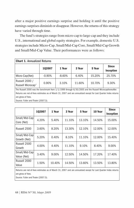
after a major positive earnings surprise and holding it until the positive

earnings surprises diminish or disappear. However, the returns of this strategy

have varied through time.

The fund’s strategies range from micro-cap to large-cap and they include

U.S., international and global equity strategies. For example, domestic U.S.

strategies include Micro-Cap, Small/Mid-Cap Core, Small/Mid-Cap Growth

and Small/Mid-Cap Value. Their performances were as follows:


Chart 1. Annualized Returns

1Q2007 1 Year 3 Year 5 YearSince

Inception

Micro-Cap(Net) -0.90% -8.60% 6.40% 15.20% 25.70%

Russell 2000 / Russell Microcap+ 0.90% 3.10% 11.60% 10.70% 9.30%

The Russell 2000 was the benchmark from 1/1/1999 through 6/30/2005 and the Russell Microcapthereafter.

Returns are net-of-fees estimates as of March 31, 2007 and are annualized except for Last Quarter Index returns

are gross-of fees.

Source: Fuller and Thaler (2007:3).

1Q2007 1 Year 3 Year 5 Year 10 YearSince

InceptionSmall/Mid-CapCore (Net)

4.20% 5.40% 11.10% 13.10% 14.50% 15.00%

Russell 2500 3.60% 8.20% 13.30% 12.10% 12.00% 12.00%

Small/Mid-CapGrowth (Net)

5.20% 0.40% 8.10% 11.10% 12.00% 15.40%

Russell 2500Growth

4.00% 4.40% 11.10% 9.10% 8.40% 9.00%

Small/Mid-CapValue (Net)

3.40% 9.00% 12.50% 14.50% 17.20% 17.40%

Russell 2000Value

1.50% 10.40% 14.50% 13.60% 13.50% 13.80%

Returns are net-of-fees estimates as of March 31, 2007 and are annualized except for Last Quarter Index returns

are gross-of fees.

Source: Fuller and Thaler (2007:3).

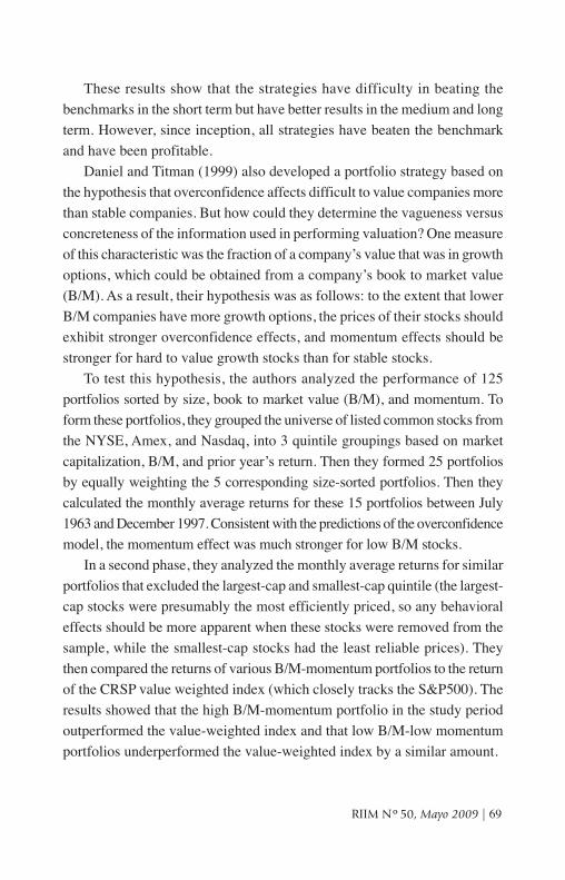
These results show that the strategies have difficulty in beating the

benchmarks in the short term but have better results in the medium and long

term. However, since inception, all strategies have beaten the benchmark

and have been profitable.

Daniel and Titman (1999) also developed a portfolio strategy based on

the hypothesis that overconfidence affects difficult to value companies more

than stable companies. But how could they determine the vagueness versus

concreteness of the information used in performing valuation? One measure

of this characteristic was the fraction of a company’s value that was in growth

options, which could be obtained from a company’s book to market value

(B/M). As a result, their hypothesis was as follows: to the extent that lower

B/M companies have more growth options, the prices of their stocks should

exhibit stronger overconfidence effects, and momentum effects should be

stronger for hard to value growth stocks than for stable stocks.

To test this hypothesis, the authors analyzed the performance of 125

portfolios sorted by size, book to market value (B/M), and momentum. To

form these portfolios, they grouped the universe of listed common stocks from

the NYSE, Amex, and Nasdaq, into 3 quintile groupings based on market

capitalization, B/M, and prior year’s return. Then they formed 25 portfolios

by equally weighting the 5 corresponding size-sorted portfolios. Then they

calculated the monthly average returns for these 15 portfolios between July

1963 and December 1997. Consistent with the predictions of the overconfidence

model, the momentum effect was much stronger for low B/M stocks.

In a second phase, they analyzed the monthly average returns for similar

portfolios that excluded the largest-cap and smallest-cap quintile (the largest-

cap stocks were presumably the most efficiently priced, so any behavioral

effects should be more apparent when these stocks were removed from the

sample, while the smallest-cap stocks had the least reliable prices). They

then compared the returns of various B/M-momentum portfolios to the return

of the CRSP value weighted index (which closely tracks the S&P500). The

results showed that the high B/M-momentum portfolio in the study period

outperformed the value-weighted index and that low B/M-low momentum

portfolios underperformed the value-weighted index by a similar amount.


Finally, they studied the performance of long-short strategies for 1964-

1997 that bought the high B/M-high momentum portfolio and sold the low

B/M-low momentum portfolio for all quintiles and then for quintile 2-4. The

performance of these portfolios was striking. The all-quintile strategy realized

an average annual return of 12.4% a year, generating profits in 31 out of 34

years in the sample period.

The main conclusion is that the evidence rejects the notion of efficient

markets in favor of an alternative theory in which asset prices are influenced

by investor overconfidence. The previous studies show that portfolio strategies

that may be suggested by the overconfidence theory can realize high abnormal

returns (which cannot be explained by additional risk). However, are these

trading strategies more profitable than other trading strategies? Are they

persistently successful? How would these strategies perform in another

sample period or in another market? Is it worth introducing overconfidence

into the models?

Overreaction

1) Identification of its main issues and propositions.

Research in experimental psychology suggests that, in violation of Bayes’

rule, most people tend to overreact to unexpected and dramatic news events,

overweighting recent information and underweighting prior data (De Bondt

and Thaler, 1985). Shefrin (1998) relates this concept to representativeness,

which he identifies as ‘one of the most important principles affecting financial

decisions, and it refers to judgments based on stereotypes’.

But how does this behavior affect stock prices? Shefrin believes that

‘investors who rely on the representativeness heuristic become overly

pessimistic about past losers and overly optimistic about past winners, and

this instance of heuristic-driven bias causes prices to deviate from fundamental

value’.

Specifically, investors overreact to both bad and good news. Therefore,

overreaction leads past losers to become underpriced and past winners to

become overpriced. However, empirical research shows that this mispricing


is not permanent; over time the mispricing corrects itself. The losers will

outperform the general market, while winners will underperform.

2) Empirical models: research designs and methodology.

Several research papers have focused on overreaction, but perhaps the most

notorious financial example illustrating representativeness and overreaction

is the winner-loser effect documented by De Bondt and Thaler (1985, 1987).

In their 1985 study, De Bondt and Thaler carried out an empirical test of

the overreaction hypothesis, trying to identify if the overreaction hypothesis

was predictive; i.e. whether it did more than merely explain, ex post, the

results on asset price dispersion. Their two hypotheses were as follows: (a)

extreme movements in stock prices will be followed by subsequent price

movements in the opposite direction; and (b) the more extreme the initial

price movement, the greater will be the subsequent adjustment. It is important

to notice that both hypotheses imply a violation of weak-market efficiency.

The basic research design used to form the winner and loser portfolios

was as follows:

• Monthly return data for New York Stock Exchange (NYSE) common

stocks for the period between January 1926 and December 1982 were

used (compiled by the Center for Research in Security Prices (CRSP) of

the University of Chicago). An equally weighted arithmetic average

return on all CRSP listed securities served as the market index.

• For every stock j with at least 85 months of return data, monthly residual

returns were estimated μjt. The procedure was repeated 16 times starting

in January 1930, January 1933,…., up to January 1975.

• For every stock j, starting in December 1932, they computed the cumulative

excess returns (CUj) for the prior 36 months. This step was repeated 16

times for all non-overlapping three-year periods between January 1930

and December 1977.

• On each of the relevant portfolio formation dates (Dec. 1932, Dec. 1935,

etc), the CUj’s were ranked from low to high and portfolios were formed.

Firms on the top decile were assigned to the winner portfolio W; firms

in the bottom decile to the loser portfolio L. In other words, the authors


formed portfolios of the most extreme winners and of the most extreme

losers, as measured by cumulative excess returns over successive three

year formation periods.

Consistent with the predictions of the overreaction hypothesis, portfolios

of prior losers were found to outperform prior winners: loser portfolios of 35

stocks outperformed the market by, on average, 19.6%, 36 months after portfolio

formation; meanwhile, winner portfolios earned about 5% less than the market,

so that the difference in cumulative average residual between the extreme

portfolios equaled 24.6% (t statistic: 2.20). In other words, thirtysix months

after portfolio formation, the losing stocks earned about 25% more than the

winners, even though the survey showed that the latter were significantly more

risky (the average betas of the securities in the winner portfolios were significantly

larger than the betas of the loser portfolio). Additionally, the tests showed that:

(i) the overreaction effect was asymmetric; it was much larger for losers than

for winners (it was reported that after the date of portfolio formation, losers

won approximately three times the amount that winners lost); (ii) stocks that

went through more (less) extreme return experiences showed subsequent price

reversals more (less) pronounced; and (iii) a strong seasonality was present

as a large portion of the excess returns occurred in January.

The interpretation of the results as evidence of investor overreaction was

questioned by Vermaelen and Verstringe (1986), who claim that ‘the

overreaction effect is a rational market response to risk changes’. Their risk-

change hypothesis states that a decline (increase) in stock prices leads to an

increase (decline) in debt-equity ratios and in risk as measured by CAPM

betas.5

Using the same data set as in their 1985 paper, De Bondt and Thaler

wrote a follow-up paper in 1987 where they address the issues of seasonality

and firm size. While trying to explain the seasonality patterns present in the

results of the 1985 paper, the authors pose the following questions: (i) Were

there any seasonal patterns in returns during the formation period?; (ii) Were

the January corrections driven by recent share price movements (say, over

the last few months), or by more long-term factors?; and (iii) Could the

winner-loser effect be explained by changes in CAPM betas?


The basic research design used to form the winner and loser portfolios

was as follows:

• For every stock j on the CRSP monthly return data (1926-1982) with at

least 61 months of return data, and starting in January 1926, they estimated

120 monthly market-adjusted excess returns, μjt = Rjt − Rmt, covering

both a five-year portfolio “formation” and a five-year “test” period. The

procedure was repeated 48 times for each of the ten-year periods starting

in January 1926, January 1927, and up to January 1973.

• For every stock in each sample, the computed the cumulative excess

returns (CUj) over the five-year formation period. After that, the CUj’s

were ranked from low to high and portfolios were formed. The 50 stocks

with the highest CUj’s were assigned to the winner portfolio W; the 50

stocks with the lowest CUj’s to the loser portfolio L. In total there were

48 winner and 48 loser portfolios, each containing 50 securities.

• For the five sequences of all non-overlapping formation periods that start

in January 1926, January 1927, and up to January 1930, the single most

extreme winners from each formation period were combined to form

group W1. The stocks that came in second in the formation period formed

group W2, etc. Consequently, they had, for each of the five experiments,

50 “rank portfolios” for winners, W1,…, W50, and 50 “rank portfolios”

for losers formed in the same way. In total there were 250 winner and

250 loser rank portfolios. Finally, average and cumulative average excess

returns were found for each rank portfolio.

The authors confirmed that seasonality was present in both the test period

returns and the formation period returns. During the test period, losers earned

virtually all of their excess returns in January, while winner excess returns

(though smaller in absolute terms than for losers), also occurred predominantly

in January. In the formation period, the January excess returns for winners

were about double that of the abnormal performance in other months. For

losers, the seasonal pattern was also present.

These results raised the question of to what extent the January returns

of long-term winners and losers were actually driven by performance over

the immediately preceding months, possibly reflecting tax-motivated trading.


The authors found that excess returns for losers in the test period (and

particularly in January) were negatively related to both long-term and short-

term formation period performance. For winners, January excess returns

were negatively related to the excess returns for the prior December, possibly

reflecting a capital gains tax “lock-in”. Additional tests and findings continued

to be consistent with tax explanations of the unusual January returns.

Regarding their last question, in their previous paper, the authors had

found out that regardless of the length of the formation period, the beta for

the loser portfolio was always lower than the beta for the winner portfolio.

However, Chan (1986) and Vermaelen and Verstringe (1986) argued that the

usual procedure of estimating betas over a prior period was inappropriate if

betas varied with changes in market value. For winners and losers, a negative

correlation between risk and market value is plausible because of changes

in financial leverage that accompany extreme movements of the value of

equity. The implication is that the winner-loser effect may disappear if the

risk estimates were obtained during the test period. They argued that De

Bondt and Thaler should have looked at the test period betas, as risk may

have changed as the losers were losing and the winners were winning. Still,

the test period betas were only slightly higher for losers than for winners

(1.263 vs 1.043) and this estimated risk difference was not capable of

explaining the gap in returns. In other words, the winner-loser effect could

not be attributed to changes in risk as measured by CAPM betas.

In regards to the size effect, De Bondt and Thaler (1987) also tried to

identify if the winner-loser effect was qualitatively different form the size

effect. In particular, they tried to answer two questions: (i) are losing firms

particularly small?; and (ii) are small firms (size measured by market value

of equity) for the most part losers? The basic research design used was as

follows:

• The sample included both NYSE and AMEX firms listed in COMPUSTAT

for the years 1966-1983.

• For each firm j, annual returns Rjt and excess returns μjt were computed

from COMPUSTAT data for all years between t−3 and t+4, with t

representing the final year of the formation period.


• Every sample was ordered by each of the following 4 rankings: (a)

cumulative excess return (CUj) over a four-year formation period between

the end of year t−4 and the end of year t; (b) market value of equity (MV)

at the end of year t; (c) market value of equity divided by book value of

equity (MV/BV); (d) company assets at t.

• For each sample and for each ranking variable, quintile, decile and ventile

portfolios were formed. Average and cumulative average excess returns

were calculated for the four years between t−3 and t, and for the four

years between t+1 and t+4.

The results showed that even for quintile portfolios, (which are less

extreme than the decile or groups of 50 stocks used in their previous study)

the losers had positive excess returns and the winners had negative excess

returns. However, they were not able to describe the winner-loser anomaly

as primarily a small firm phenomenon. On the other hand, they were able

to show that the size effect, as measured by MV, was partly a losing effect;

i.e. there was a relationship between the size effect and the losing firm effect.

The firms in the loser portfolios had lost a substantial portion of their value.

Since the firm size is usually measured by the MV of equity, the losing firms

became much smaller during the formation period.

In short, the results showed that (i) the winner-loser effect is not primarily

a size effect; (ii) the small firm effect is partly a losing firm effect, but even

if the losing firm effect is removed by using a more permanent measure of

size, such as assets, there are still excess returns to small firms; and (iii) the

earnings of winning and losing firms showed reversal patterns that were

consistent with overreaction.

Following the results from their 1987 paper, De Bondt and Thaler (1989)

referred to the concept of mean reversion.6 The idea that systematic

“irrationality” in investors’ attitudes may affect prices, and that prices may

deviate from fundamental value, raised the following question: do stock

prices follow a random walk or are they somewhat predictable?

The efficient market view claims that stock prices quickly and rationally

reflect all public information; i.e. stock prices follow a stochastic process close

to a random walk. On the other hand, the overreaction hypothesis admits to


temporary disparities between prices and fundamentals. So De Bondt and

Thaler tried to show that if overreaction was present in financial markets, then

we should observe mean-reverting returns to stocks that have experienced

extremely good or bad returns over the past few years. Referring to the 1985

paper, they showed that (i) the returns for both winners and losers were mean-

reverting; and (ii) the five-year price reversal for losers was more pronounced

than for winners. In addition, and consistent with overreaction, they showed

that the more extreme the initial price movements, the greater the subsequent

reversals. Additionally, they tested mean reversion in the short term. If mean

reversion was observed over very brief time periods, factors other than size

or objective risk could be assumed to be at work.7 Basing their analysis on the

study carried out by Bremer and Sweeny (1988), they showed that there was

a significant correction for losers in the short term, but not for winners, and

that the correction increased with the size of the initial price jump.

Several conclusions follow from these results8 but the main one is that

although prices may deviate from fundamental value, eventually, they get

corrected as actual future events predictably turn out to be more or less than

expected. A consequence for portfolio management is that this price behavior

explains the profitability of contrarian strategies. Contrary to market efficiency,

prior stock market “losers” are much better investments than prior “winners”.9

In a later work, De Bondt and Thaler (1990) present a study of the

expectations of security analysts who make periodic forecasts of individual

company earnings. They specifically test for a type of generalized overreaction,

the tendency to make forecasts that are too extreme, given the predictive value

of the information available to the forecaster. Their focus is on forecasted

changes in earnings per share (EPS) for one and two year time horizons. In

particular, they tried to answer the following questions: Are forecast errors in

EPS systematically linked to forecasted changes? Are the forecasts too extreme

(so actual changes are less than predicted)? Are most forecast revisions “up”

(“down”) if the analysts’ initially projected large declines (rises) in EPS?

(Under rationality, neither forecast errors nor forecast revisions should ever

be predictable form forecasted changes). Does the bias in the forecasts get

stronger as uncertainty grows and less is known about the future?


In order to answer these questions, they used the following research

design:

The analysts’ earnings forecasts between 1976 and 1984 were taken from

the Institutional Brokers Estimate System tapes (IBES) produced by Lynch,

Jones & Ryan. They worked only with the April and December predictions

of EPS for the current as well as the subsequent year. They matched the

earnings forecasts for each company with stock returns and accounting

numbers as provided by the CRSP at the University of Chicago and the

annual industrial COMPUSTAT files. Most of the regression analysis was

based on three sets of variables: forecasted changes in EPS, actual changes

in EPS, and forecast revisions.

The results of the study showed that forecasts were too optimistic, too

extreme, and even more extreme for two-year forecasts than for single-year

predictions. They also showed that forecast revisions were predictable from

forecasted changes, violating the rationality assumption. In sum, the results

were consistent with generalized overreaction.

The authors’ main conclusion is that even the predictions of security

analysts, who may be considered a source of rationality in financial markets,

present the same pattern of overreaction found in the predictions of naïve

undergraduates. Forecasted changes are simply too extreme to be considered

rational.

Along the same lines, De Bondt (1991) continued to analyze regression

to the mean in the belief that strategists are prone to committing gambler’s

fallacy, a phenomenon were people inappropriately predict reversal. Gambler’s

fallacy is regression to the mean gone overboard (overreaction). His survey

examined the market prediction collected by Joseph Livingston since 1952.10

In particular, he examined about 5400 individual forecasts of the S&P index

and of 425 industrial companies for the period between 1952 and 1986. The

time horizon was seven and thirteen months.

In accordance with gambler’s fallacy, De Bondt found that these predictions

consistently were overly pessimistic after a bull market and overly optimistic

after a bear market. In particular, the results showed that, after three-year

bull markets, economist predicted that on average, over the next seven


months, the S&P would decline at an annual rate of 6.4%. He concluded

that this pessimism was not borne out by the facts even though actual returns

turned out to be much smaller after large price run-ups than after market

declines. Actual returns were less than expected returns if the market was

expected to rise and more than expected if a decline was predicted.

The results also showed that professional economists expected reversals

in stock prices. After three-year bull markets, on average, 52.6% of the

subjects saw a weak downward trend. The equivalent number for three-year

bear markets was only 17.8%. But a curious finding is that these results on

mean reversion in stock prices were unknown to the survey participants; i.e.

they did not know that the average economist is a contrarian, pessimistic in

bull markets and optimistic in bear markets.

De Bondt continued by asking the following question: What does

regression to the mean suggest about predictions in the wake of above-

average performance? He concluded that it implies that future performance

will be closer to the mean, not that it will be below the mean in order to

satisfy the law of averages.

Up to this point, academic research provided us with evidence of medium

to long term reversals. Lehman (1990) argues that shorter-term reversals can

also be observed.11 Lehman believes that predictable variations in equity

returns may reflect either predictable changes in expected returns or market

inefficiency and stock price overreaction. He believes that these explanations

can be distinguished by examining returns over short time intervals since

systematic changes in fundamental valuation over intervals like a week

should not occur in efficient markets. He argues that ‘asset prices should

follow a martingale process over short time intervals even if there are

predictable variations in expected security returns over longer horizons

–systematic short-run changes in fundamental values should be negligible

in an efficient market with unpredictable information arrival’. As a consequence,

rejection of this martingale behavior over short horizons would be evidence

against market efficiency.

Lehman tested the market efficiency hypothesis by examining security

prices for evidence of unexploited arbitrage opportunities. His model was


based on the assumption that any stock price overreaction infects many

securities returns. Consequently, well-diversified portfolios composed of

either “winners” or “losers” might be expected to experience return reversals

in these circumstance. As a result, he developed a simple strategy to test

market efficiency: he studied the profits of costless (i.e. zero net investment)

portfolios which gave negative weight to recent winners and positive weight

to recent losers. The short run martingale model predicted that these costless

portfolios should earn zero profits. In contrast, if stock prices did overreact,

violating the efficient market hypothesis, these costless portfolios would

typically profit from return reversals over some horizon.

The research design implemented was as follows: Equity securities listed

on the New York and American Stock Exchange were used from 1962 to

1986. Portfolio weights were taken to be proportional to the difference

between the return of security i and the return on an equally weighted portfolio

at different lags; i.e. the number of dollars invested in each security was

proportional to the return in week k less the return of the equally weighted

portfolio. A week was considered to be a sufficiently short period for the

martingale model to apply under the efficient market hypothesis; i.e. weekly

security returns were used. Profits were reported for five horizons: one, four,

thirteen, twenty six and fifty two weeks.

The results of this study strongly suggest rejection of the efficient market

hypothesis. His results showed that the “winners” and “losers” one week

experienced sizeable return reversals the next week in a way that reflected

arbitrage profits. In other words, portfolio of securities that had positive

returns in one week typically had negative returns in the next week, while

those with negative returns in one week typically had positive returns in the

next week. The costless portfolio that is the difference between the winners

and losers portfolios had positive profits in 90% of the weeks.

However, the results failed to find pronounced persistence in the return

reversal effect. On average, the winner portfolio only had negative mean

returns in the subsequent week but had positive and increasing mean returns

over the next month. Similarly, the loser portfolio had large positive mean

returns in the subsequent week but they diminished over the next month.


3) Strength and weakness analysis: Were the research methods appropriate

to measure overreaction? What questions have been left unanswered?

In conclusion, the overreaction hypothesis believes that, in violation of Bayes’

rule, most people tend to overreact to unexpected and dramatic news events,

overweighting recent information and underweighting prior data. The winner-

loser effect documented by De Bondt and Thaler is, perhaps, the most

illustrative example of overreaction. Their work, as well as the research that

followed, is successful in proving that investors overreact. The research

designs were appropriate and the questions that arose as a result of one

publication was answered in following papers, either by the same authors

or by other researchers.

However, the empirical analysis showed some limitations and several

questions have not yet been answered. These issues can be grouped into four

broad considerations:

First: Can overreaction explain the behavior in stock prices and returns?

De Bondt and Thaler (1985) argue that mean reversion is evidence of

overreaction. They showed that over the 3 to 5-year holding period, stocks

that performed poorly over the previous 3 to 5 years achieve higher returns

than stocks that performed well over the same period. In the 1987 paper

they showed that these excess returns could not be easily attributed to

changes in risk or the “small firm anomaly”. 12 However, as stated by

Jegadeesh and Titman (1993), De Bondt and Thaler’s results are still being

debated.

In De Bondt and Thaler (1985), the winner and loser portfolios were

formed conditional upon past excess returns, rather than some firm-generated

informational variable such as earnings. But can past returns be considered

good predictors of future returns? Additionally, the requirement that 85

subsequent returns were available before any firm was allowed in the sample

biased the selection towards large, established firms. Consequently, can these

results be generalized?

De Bondt and Thaler also showed that 36 months after portfolio formation,

the losing stocks earned about 25% more than the winners, even though the

survey showed that the latter were significantly more risky (the average betas


of the securities in the winner portfolios were significantly larger than the

betas of the securities in the loser portfolio). The authors identified this issue

but failed to explain why this happened. In other words, is it correct to assume

that the risk-return relationship implicit in the efficient markets hypothesis

was violated? And what can be implied by these results? However, in trying

to solve this issue and also answer the question raised by Chan (1986) and

Vermaelen and Verstringe (1986) that the winner-loser effect may disappear

if the risk estimates were obtained during the test period, their 1987 paper

found that the test period betas were only slightly higher for losers than for

winners and that this estimated risk difference was not capable of explaining

the gap in returns. In other words, they showed that if the CAPM beta is an

adequate risk measure, then the difference between the winner and the loser

returns could not be attributed to differences in risk.

Some final comments refer to asymmetric overreaction and seasonality.

The authors identified that the overreaction effect was asymmetric, but they

failed to explain why. Additionally, although the authors offered an explanation

of the strong seasonality present in their results, significant research had to

follow in order to explain this phenomenon.

Second: Is mean reversion a sign of market inefficiency? And are contrarian

strategies the answer? The fact that prices are mean reverting implies that

prices are predictable. But as stated by Fama and French (1986), does

predictability reflect market inefficiency or time-varying expected returns

generated by rational investor behavior? Mean reversion can also explain

the profitability of contrarian strategies. In particular, Lehman’s results (1990)

showed that the “winners” and “losers” one week experienced sizeable return

reversals the next week in a way that reflected arbitrage profits. In particular,

relative strength strategies that bought past winners and sold past losers have

been documented to show significant abnormal returns13 (practitioners in

USA still use this strategy as one of their stock selection criteria (Grinblatt

and Titman, 1989, 1993). These results strongly suggested rejection of the

efficient market hypothesis. But do these contrarian strategies offer consistent

abnormal returns over other strategies? Is it profitable always to invest using

contrarian strategies?


Moreover, the evidence on short-term reversals presented by Jegadeesh

(1990) and Lehmann (1990) can also be criticized. These papers show that

contrarian strategies that select stocks based on their returns in the previous

week or month generate significant abnormal returns. However, since these

strategies are based on short-term price movements, their apparent success

may reflect the presence of short-term price pressure or a lack of liquidity

in the market rather than overreaction.14 Additionally, the explanation of

why there is little persistence in the return reversal effects is not sufficient.

Lehman offers two possible explanations: ‘first, one could emphasize the

short-run nature of the arbitrage opportunity and presume that equity markets

are (on average) efficient over longer horizons….alternatively, one could

emphasize the low power of the tests for detecting longer tem market

inefficiencies and continue to seek additional evidence (and reinterpret

existing evidence) of market inefficiency’. However, further analysis is

needed to address this issue in full.

Third: What causes the overreaction phenomenon; in other words, what

causes the systematic excessive optimism or pessimism present in forecasters?

De Bondt and Thaler (1990) showed that EPS forecasts were too optimistic

and too extreme. However and even though they tried to explain the EPS

forecast error, they failed to identify the causes of this excessive optimism

or pessimism in earnings forecasts. This same question was also present in

De Bondt’s 1991 survey. The author offered some explanations, focusing

on expected inflation, expected real economic growth, the S&P price-earnings

ratio on the forecast date, and the three-year cumulative historical returns

immediately prior to the forecast. Another explanation of this behavior has

been offered by Shefrin (1998): Regret and hindsight bias come together in

the selection of loser stocks for a portfolio: people are fearful of investing

in loser stocks, although evidence has shown that a portfolio of losers

historically outperformed the market. But these explanations are not

satisfactory; further research is necessary.

Fourth: How does the overreaction hypothesis affect portfolio theory

and portfolio selection; i.e. how can these anomalies be incorporated into

existing models? The proponents of market efficiency hold that there are


enough well-informed investors to seize all unexploited profit opportunities.

The evidence from behavioral decision-making studies is that people learn

slowly. So, are there enough quick learners to eliminate mispricing in financial

markets? DeBondt and Thaler believe that because of representativeness,

investors become overly optimistic about recent winners and overly pessimistic

about recent losers. Hence, they propose buying past losers and selling past

winners. If prices either overreact or underreact to information, then profitable

trading strategies that select stocks based on their past returns will exist,

achieving abnormal returns.

However, strategies based on relative strength have also been proven to

show abnormal returns.15 In 1993 Jegadeesh and Titman documented the

strategies that bought stocks that had performed well in the past and sold

stocks that had performed poorly in the past. In other words, the authors

tested the inverse trading strategy proposed by DeBondt and Thaler in 1985.

In particular, Jegadeesh and Titman (1993) provided an analysis of relative

strength trading strategies over 3 to 12 month horizons (in each month t, the

strategy bought the winner portfolio and sold the loser portfolio). Their

results showed that: (i) trading strategies that bought past winners and sold

past losers realized significant abnormal returns over the 1965 to 1989 period;

(ii) the profitability of the relative strength strategies was not due to their

systematic risk; (iii) profits could not be attributed to a lead-lag effect resulting

from delayed stock price reactions to information about a common factor,

although the evidence was consistent with delayed price reactions to firm-

specific information; (iv) part of the predictable price changes that occurred

during the 3 to 12 month holding periods may not have been permanent (the

longer-term performances of the past winners and losers revealed that half

of their excess returns in the year following the portfolio formation date

dissipated within the next 2 years).

So, which trading strategy is more profitable? Can they be compared?

Jegadeesh and Titman (1993) offered an explanation: the discrepancy between

the results of both trading results may be due to the difference between the

time horizons used in the trading rules examined in the academic papers and

those used in practice. For example, they cited evidence favoring contrarian


strategies focusing on trading strategies based on either very short-term return

reversals (1 week or 1 month), or very long-term return reversals (3 to 5 years).

However, evidence suggested that practitioners who use relative strength rules

base their selection on price movements over the past 3 to 12 months.16

Another alternative that has been proposed is the study of the excess

returns from value investing. Graham and Dodd (1934) found that excess

returns were obtainable from a low P/E strategy. The results showed that

buying stocks with low P/E led to excess risk-adjusted returns, and the

extreme losers outperformed the market. This strategy was replicated in the

United States and Japan, showing similar results.17

Taking all this into account, is it worth incorporating these anomalies

into existing models? I believe it is but further research that attempts to

identify explanations for these empirical irregularities is necessary. As De

Bondt and Thaler (1989) state, ‘the real challenge facing the field (of finance)

is to develop new theories of asset pricing that are consistent with known

empirical facts and offer new testable predictions’. The authors suggest

models in which some agents have non-rational expectations of future cash

flows, or have faulty risk perceptions (versus traditional models in which

all agents are assumed to be fully rational).

IV. Implications of overconfidence and overreaction for marketefficiency and investors’ rational behavior and the responses given bythe Traditional Finance Theory

In the above discussion, it was implied that the presence of overconfidence

and overreaction in investors’ choices affects the efficient market hypothesis

and may cause prices to deviate from fundamental value. However, Traditional

Finance Theory has addressed some of these issues and several responses

have been given. As a result, the objective of this section is to analyze the

implications of the anomalies regarding overreaction and overconfidence

for market efficiency, rational behavior and fundamental value, and to analyze

the responses given by the Traditional Finance Theory.


Let’s recall that the traditional theory of finance assumes that individuals

are rational; i.e. they develop expectations using Bayesian strategies and

make optimal decisions based on the available information. As a result, prices

reflect all available information, so opportunities to earn extraordinary returns

arise only from new information. Since the arrival of unexpected information

is random, prices will follow a random walk and returns will be normally

distributed (i.e., the entire return distribution can be described by its mean

and its standard deviation).

As Fama (1970) explains, on the one hand, it is easy to determine sufficient

conditions for capital market efficiency, such as: (i) the lack of transaction

costs in trading securities; (ii) all available information is costlessly available

to all market participants; and (iii) all agree on the implications of current

information for the current price and distributions of future prices of each

security. In this world, Fama sustains that it is easy to assume that the current

price of a security fully reflects all available information.

However, a market with these conditions is not met in practice. As a

result, numerous studies have tested the efficient market hypothesis throughout

the years. Testing market efficiency is basically straightforward: using

statistical methods, investigate whether a strategy (based on a certain kind

of information) consistently earns abnormal profits. Some examples included:

(1) tests of technical trading rules; (2) earnings, dividends and split

announcements; (3) trading performance of insiders (results from trading

on public information about insider trades) (Daniel, 2002).

As Fama (1970) explains, the initial studies were concerned with “weak

form” tests in which the information set was just historical prices. In the

early literature, discussions of the efficient markets model were phrased in

terms of the random walk model. The impetus for the development of a

theory came from the accumulation of evidence in the middle 1950’s and

early 1960’s that the behavior of common stock and other speculative prices

could be well approximated by a random walk. Faced with the evidence,

economists offered some rationalization, which resulted in a theory of efficient

markets stated in terms of random walks.

When the tests seemed to support the efficiency hypothesis at this level,


attention was turned to “semi strong form” tests in which the concern was

whether current prices “fully reflected” all obviously publicly available

information. Each individual test, however, was concerned with the adjustment

of security prices to one kind of information generating event (e.g. stock

splits, announcements of financial reports by firms, new security issues,

etc.).

By the time Fama wrote his 1970 paper, “strong form” tests had begun

to appear. The strong form tests of the efficient markets model were concerned

with whether all available information was fully reflected in prices in the

sense that no individual had higher expected trading profits than others

because he had monopolistic access to some information.

Lehmann (1990) also referred to this issue and explained that testing of

the efficient market hypothesis was abundant. Earlier studies supported the

random walk model, finding that the predictable variation in equity returns

was both economically and statistically small. More recently, however,

several studies began to document other examples of how market efficiency

could be violated. For example, as Fama (1991) explains, a precondition for

the strong version of the efficient market hypothesis is that information and

trading costs, the costs of getting prices to reflect information, are always

0. Since there are surely positive information and trading costs, the extreme

version of the market efficiency hypothesis is surely false.

Additionally, recent research has found evidence that equity returns can

be predicted with some reliability. In other words, there is evidence on the

predictability of daily and weekly returns from past returns.

As Raghubir and Ranjan Das (1999) state, the findings of persistent

deviation of stock prices from fundamentals are robust, suggesting that the

behavioral cause behind these price deviations is overreaction, which implies

that stock prices do not display a random walk but rather display return

predictability (Shiller, 1981, and Shleifer and Vishny, 1990).

Lehman argues that there are two competing explanations for this

phenomenon. The first is that the returns vary through time, resulting in

predictable, but efficient, mean reversion in stock prices. On the other hand,

the predictability of equity returns may reflect the overreaction of stock


prices, as suggested by De Bondt and Thaler. But these two explanations

can be distinguished by examining asset returns over short time intervals.

As explained in the previous section, Lehman tested this hypothesis and the

results showed that the “winners” and “losers” one week experienced sizeable

return reversals the next week in a way that reflected arbitrage profits. The

results of this study strongly suggest rejection of the efficient market

hypothesis. Additionally, Shiller (1979) argues that there is more volatility

in stock markets and bond markets than would be the case if prices were

determined by fundamental value alone.

In other words, the evidence of systematic reversals in stock returns over

the short and long-term violates the efficient market hypothesis. In response

to these studies, Fama reviewed once again the market efficiency literature

in 1991, offering his views on what he had learned from the research on

market efficiency.

The 1991 review also divided work on market efficiency into three

categories, but they somewhat differed from the categories identified in the

1970 paper. The main difference was in the first category: instead of weak

form tests (which are only concerned with the forecast power of past returns),

the first category covered the more general area of tests for return predictability,

which also included the work on forecasting returns with variables like

dividend yields and interest rates. For the second and third categories, he

only proposed changes in title, not coverage, naming them event studies and

tests for private information, respectively.

Fama (1991) stated that ‘ambiguity about information and trading costs

is not the main obstacle to inferences about market efficiency’. He believed

that the joint-hypothesis problem was more serious. Thus, market efficiency

per se is not testable; it must be tested jointly with some model of equilibrium,

an asset pricing model. This point says that one can only test whether

information is properly reflected in prices in the context of a pricing model

that defines the meaning of “properly”. As a result, he concluded that when

one ‘finds anomalous evidence on the behavior of returns, the way it should

be split between market inefficiency or a bad model of market equilibrium

is ambiguous’.


Finally, Fama also raised a very important question: Does return

predictability reflect rational variation through time in expected returns,

irrational deviations of price from fundamental value, or some combination

of the two? Additionally, Fama (1998) stated that it was time to ask whether

the recent studies on long-term returns that suggested market inefficiency

also suggested that efficiency should be discarded. His answer was a strong

no: an efficient market generates categories of events that individually suggest

that prices overreact to information. But in an efficient market, under-reaction

will be about as frequent as overreaction. If anomalies split randomly between

under-reaction and overreaction, they are consistent with market efficiency.

Thaler (1999) also addressed this issue. On the one hand, he believes

that real financial markets do not resemble the ones one could imagine if

we only read finance textbooks. But, on the other hand, he sustains that there

is compelling evidence that markets are efficient, and that is the performance

of active fund managers. In short, he believes that although market behavior

often diverges from what would be expected in a rational efficient market,

these anomalies do not create such large profit opportunities so that active

fund managers as a group can earn abnormal returns.

However, an alternative explanation for why active money managers

may underperform passive money managers can be offered based on

overconfidence. Odean (1998) believes that active money managers may be

overconfident in their ability to beat the market and spend too much time

and money trying to do so. When information is costly, overconfident traders

who actively pursue information fare less well than passive traders.

Can the efficient market hypothesis be discarded?

An important defense against market efficiency is that the anomalies literature

has not settled on a specific alternative to market efficiency; it only points

out that market inefficiency occurs. For example, the anomalies literature

has not accepted the discipline of overreaction to be the prediction of a

behavioral finance alternative to market efficiency. If apparent overreaction

was the general result in studies of long-term returns, market efficiency


would be dead, replaced by the behavioral alternative of overreaction.

However, the anomalies literature has found that under-reaction is about as

frequent. For example, there is evidence that stock prices seem to respond

to earnings announcements for quite some time after they are announced

(post earnings announcement drift and post recommendation drift).18

The market efficiency hypothesis offers an answer to the question regarding

why the market overreacts in some instances and under-reacts in others, and

that is chance. As Fama (1998) explains, ‘the expected value of abnormal

returns is zero, but chance generates apparent anomalies that split randomly

between overreaction and under-reaction. In other words, Fama believes that

apparent overreaction of stock prices to information is about as common as

under-reaction, and this is consistent with the market efficiency hypothesis

that the anomalies are chance results (although “behavioralists may argue

that it is possible to distinguish chance from systematic cognitive bias because

the behavioral literature does not simply say that people do not behave exactly

as the traditional model predicts; it says that people behave in specific,

regular, predictable ways that are inconsistent with the traditional models).

As a result, Fama (1998) believes that the behavioral literature does not

lean cleanly towards either anomaly (under-reaction vs. overreaction) as the

behavioral alternative to market efficiency. So, is the weight of the evidence

on long-term return anomalies so big that market efficiency is not a viable

working model even in the absence of an alternative model that explains

both under and overreaction?

Thaler (1999) also refers to this issue. Even though his 1999 study shows

that the premise of behavioral finance –that cognitive biases may influence

asset prices-is at least theoretically possible, he wonders if it is worth the

trouble. Specifically, he wonders: What is the evidence that traditional models

cannot do the job? In other words, is there enough evidence to undermine

the rational efficient market paradigm?

Statman (1999) also believes that market efficiency is at the center of

the battle between standard finance and behavioral finance, and that

overreaction and under-reaction are “weapons” in this battle. But he continues

by making a distinction between two meanings of the term “market efficiency”.


One meaning is that investors cannot systematically beat the market. The

other is that security prices are rational. Rational prices reflect only utilitarian

characteristics, such as risk, not value expressive characteristics, such as

sentiment. He continues by stating that behavioral finance has shown, however,

that value-expressive characteristics matter in both investor choices and asset

prices. Therefore, the market efficiency battle is being fought as if one side

can only win if the other loses. Statman believes that ‘the discipline of finance

would do well to accept the first meaning of market efficiency and reject

the notion that security prices are rational…we could then stop fighting the

market efficiency battle and focus on exploring (i) asset pricing models that

reflect both value expressive and utilitarian characteristics and (ii) the benefits,

both utilitarian and value expressive, that investment professionals provide

to investors’. He concludes by arguing that today’s standard finance is so

weighted down by anomalies that reconstructing financial theory along

behavioral lines makes a lot of sense. But, as Ray Ball explains (Chew, 1999),

‘the theory of efficient markets was an audacious and welcome change from

the comparative ignorance of stock markets behavior that preceded it: and

despites its now obvious theoretical and empirical flaws, it has profoundly

influenced both the theory and practice of finance’.

What does Behavioral Finance have to offer?

Given such limitations in the concept of market efficiency and the existing

empirical tests of the theory, a group of finance scholars known as

“behavioralists” has suggested that it is time to abandon the premise of

collectively rational investors on which the theory rests. “Behavioralists”

argue that stock price corrections and cycles reflect systematic biases in how

investors use information (Chew, 1999). But is behavioral finance the answer

to the limitations of the efficient markets theory?

What we do know is that Behavioral Finance offers an alternative paradigm

to the efficient market theory, one in which individuals make systematic

mistakes in the way they process information (Daniel and Titman, 1999).

The main conclusion is that investors’ behaviors can influence asset


prices. Investors do not behave with extreme rationality and research has

shown that investors’ deviations from rationality are often systematic. The

main advantage of Behavioral Finance is that it relaxes the traditional

assumptions of financial economics by incorporating these observable,

systematic, and human departures from rationality into standard models of

financial markets (Barber and Odean, 1999).

Thaler (1999) also believes that behavioral finance enriches the

understanding of financial markets by ‘adding a human element’. But can

behavioral finance be theorized? Thaler mentions three groups of authors

(Barberis, Shleifer, and Vishny 1998; Daniel, Hirshleifer, and Subrahmanyam

1998; Hong and Stein 1999) who have generated asset-pricing models that

try to explain the pattern of the latest empirical results: returns that exhibit

under-reaction in the short run and overreaction in the long run. These studies

draw on results from psychology to motivate the behavior of the agents in

their models. As a result, financial economists are becoming accustomed to

thinking about the role of human behavior in driving stock prices.

V. Behavioral Finance: Future Steps for Research

So, what are the next steps Behavioral Finance should follow? Today, research

has increased and there is abundant evidence that violates the traditional

finance theory. However, there is still no widely used model that incorporates

all these anomalies. Several models have been proposed that take into account

different behavioral factors, but none of them is as popular as, for example,

the CAPM once was. Consequently, and following Statman’s (1999) advice,

the existing behavioral models should continue to be analyzed, making

adjustments as new anomalies or new criticisms to the existing models appear.

The idea of Behavioral Finance is to extend the models of financial

markets by incorporating the imperfections that we observe in the market.

But how can these factors be incorporated in the models? Shefrin and Statman

(1994) developed a behavioral asset pricing theory as an analog to the standard

CAPM. The behavioral asset pricing model (BAPM) features the market


interaction of two groups of traders: information traders and noise traders.

Information traders are the ones present in the standard CAPM and they are

free of cognitive errors and have mean-variance preferences. Noise traders

live outside the CAPM, commit cognitive errors, and do not have strict mean-

variance preferences.

The expected returns of securities in the BAPM are determined by their

“behavioral betas”, which are relative to the tangent mean-variance efficient

portfolio. But the mean-variance efficient portfolio is not the market portfolio

because noise traders affect security prices.

When prices are efficient, security prices and volatility are determined

through a single driver, a sufficient statistic consisting only of new information.

The single driver drives the mean-variance efficient frontier, the return

distribution of the market portfolio, the premium for risk, the term structure,

and the price of options. However, noise traders act as a second driver and

they steer the market away from price efficiency. When prices are inefficient,

new information is no longer a sufficient statistic. Old information continues

to affect prices, volatility, the premium for risk, the term structure and the

option prices.

In 1995, these same authors used a behavioral method of security valuation

to better understand size and book-market ratios, and beta and its correlation

to stock returns. The study provided empirical evidence on how investors

reached expectations about stock returns and related the data to realized returns.

In 1996, Fama and French developed the “three factor model” to try to

explain behavioral factors. Previous work had shown that average returns

on common stocks were related to firm characteristics like size, earnings/price,

cash flow/price, book to market equity, past sales growth, long term past

return, and short term past returns. Because these patterns in average returns

were apparently not explained by the CAPM, they were called anomalies.

The authors found that, except for the continuation of short term returns, the

anomalies largely disappeared in the three factor model. Although this model

could not explain the continuation of short term returns documented by

Jegadeesh and Titman (1993), they captured the reversal of long term returns

documented by De Bondt and Thaler (1985, 1987).


In 1999, Shefrin and Statman developed a behavioral portfolio theory as

an alternative to the Markowitz mean-variance portfolio. Mean variance

investors evaluate portfolio as a whole; they consider covariances between

assets as they construct their portfolios. They also have consistent attitudes

towards risk; they are always risk averse. Behavioral investors build portfolios

as pyramids of assets, layer by layer. The layers are associated with particular

goals and attitudes towards risk. Some money is in the downside protection

layer, designed to avoid poverty, and other is in the upside potential layer,

designed for a shot at being rich.

Finally, another factor that has been largely documented by the behavioral

finance literature and incorporated in their models is sentiment. According

to Behavioral Finance, sentiment is the reflection of heuristic-driven bias.

For example, in 1998, Barberis, Shleifer and Vishny presented a model of

investor sentiment, which was consistent with the empirical findings. In

other words, their work tried to model how investors formed beliefs. The

model was based on psychological evidence and produced both under-reaction

and overreaction for a wide range of parameter values.

Moreover, several sentiment indexes were developed to measure sentiment

in the market. Traditionally, market sentiment is seen as a contrarian indicator.

Markets rise, the theory goes, as bears become bulls and put money into the

market. The market peaks when there are no bears left and everyone is

invested. As a result, The Bullish Sentiment Index (# bulls / (# bulls + #

bears) is used as a contrarian indicator. Research shows that the BSI provides

no guidance as to where the market is headed next but it does a good job of

predicting the past.19

Moving Forward

As Merton (1987) emphasizes, ‘anomalous empirical evidence has indeed

stimulated wide-ranging research efforts to make explicit the theoretical and

empirical limitations of the basic finance model with its frictionless markets,

complete information, and rational, optimizing economic behavior…but

although much has been done, this research line is far from closure’. In short,


future research should focus in comparing the existing behavioral models

and strategies with the traditional model, trying to answer the following

questions: (1) How are portfolios designed in practice? (Active management)

(2) Do these portfolios deviate from the “efficient portfolios” identified by

the Markowitz model? Are behavioral models taken into account in portfolio

selection? (3) How do “behavioral models and strategies” behave compared

to the traditional model and to active management; i.e. which portfolio

strategy delivers superior performance? (4) Are contrarian strategies the

answer? (5) How does passive management compare to these results? (6)

Do the results vary with the sample period? (7) What happens if these models

are tested in less efficient markets such as Argentina? (8) Is it worth

incorporating behavioral factors into models?

In order to answer the first two questions, the way fund managers construct

their portfolios in practice could be analyzed. Natalia del Águila and María

Galli (1998) showed that fund managers (not only from Argentina but also

from Europe and the United States) did not use the model developed by

Markowitz to form their portfolios, claiming that the main setback of this

model was the estimation of the stocks’ expected returns.

Additionally, the research on Active Management has increased

considerably over the years. According to this research, instead of using

traditional models of portfolio selection, fund managers implement Active

Management. This method consists in several steps: (1) choosing the type

of analysis to be used in security selection, which can be strictly fundamental,

strictly technical, or a combination of both; (2) deciding if the fundamental

analysis should follow a “Top Down” or “Bottom Up” approach; and (3)

choosing the investment criteria to be followed (value vs. growth).

Future research should try to find out if, as a result of the growing literature

in behavioral finance, behavioral models are now taken into account in

portfolio selection. Then, behavioral models and strategies should be compared

to the traditional model and to active management, trying to address which

portfolio strategy delivers superior performance and if it is worth incorporating

behavioral factors into the models.

For example, a potential empirical study could be as follows:


1. Traditional Model: in order to test the traditional model, portfolios created

according to Markowitz’s portfolio optimization model could be used.

The inputs necessary to calculate the efficient frontier are expected return

and volatility of each stock, as well as the correlation between them.

Prices for stocks listed in the New York Stock Exchange (NYSE) for the

period starting in January 1990 could be used to calculate these inputs,

and the “PCF Toolkit” software could be used to calculate the efficient

portfolios.

2. Active Management: the return of US Equity Mutual Funds could be

considered to test the performance of Active Management over the years

and to be able to compare it to alternative models.

3. “Behavioral” Strategies: to test the behavioral strategies, several tests

could be carried out. To test for overconfidence, the approach used by

Barber and Odean (1999) could be replicated. In their paper, they tested

whether investors with accounts at discount brokerages traded excessively.

Their approach was to determine whether the securities bought by the

investors outperformed those they sold by enough to cover the costs of

trading. They examined return horizons of 4 months, one year and two

years following each transaction. This same methodology could be applied

to US equity mutual funds, analyzing if the securities they buy outperform

the ones they sell by enough to cover trading costs. Additionally, different

time horizons could be used, analyzing the responses in the short, medium

and long term.

In order to test for overreaction, the work done by De Bondt and Thaler

(1985) could be extended. Their two hypotheses were that extreme movements

in stock prices would be followed by subsequent price movements in the

opposite direction, and that the more extreme the initial price movement,

the greater would be the subsequent adjustment. In order to test these

hypotheses, portfolios of the most extreme winners and most extreme losers

could be formed (winner and loser portfolios) using return data for New

York Stock Exchange (NYSE) common stocks for the period starting in

January 1990. Furthermore, to address the issue of the relationship between

risk and return, portfolio CAPM betas could also be compared.


To test for mean reversion, De Bondt and Thaler’s work (1989) as well

as Lehman’s work (1990) could be extended. The former showed that (i) the

returns for both winners and losers were mean-reverting; and (ii) the five-

year price reversal for losers was more pronounced than for winners. In

addition, and consistent with overreaction, they showed that the more extreme

the initial price movements, the greater the subsequent reversals. Lehman

(1990) showed that short term reversals could also be observed. His results

showed that the “winners” and “losers” one week experienced sizeable return

reversals the next week in a way that reflected arbitrage profits. Consequently,

and in order to test for short, medium and long term price reversal, portfolios

composed of either winners or losers should be tested over a specific time

horizon, which could include 1 week, 3 months, 6 months, 12 months, 3

years and 5 years. The sample data mentioned in the previous point could

be used to form the portfolios.

Also, and based on the previous findings, contrarian and relative strength

strategies should be evaluated. Contrarian strategies consist in buying past

losers and selling past winners. On the other hand, relative strength strategies

consist in buying past winners and selling past losers. Jegadeesh and Titman

(1993) tested the inverse trading strategy proposed by De Bondt and Thaler

in 1985 (contrarian strategy), providing an analysis of relative strength

trading strategies over 3 to 12 month horizons. The results of the study

showed that trading strategies that bought past winners and sold past losers

realized significant abnormal returns over the 1965 to 1989 period. So,

which trading strategy is more profitable? In order to be able to compare

them, the time horizons used in both strategies should be the same. For

example, trading strategies based on very short-term return reversals (1

week or 1 month), or very long-term return reversals (3 to 5 years) as well

as strategies based on price movements over the past 3 to 12 months should

be considered.

Finally, additional tests could (i) compare these results to the performance

of passive management; (ii) evaluate the performance of these strategies if

the sample period is changed; and (iii) replicate the analysis in less efficient

markets such as Argentina.


In conclusion, the major factors driving portfolio selection are much

more complex than the mean and variance of future returns and the efficient

frontier. Empirical research has shown that, when selecting a portfolio,

investors not only consider statistical measures such as risk and return, but

also psychological factors such as sentiment, overconfidence and overreaction.

In short, heuristic-driven bias, frame dependence, and market inefficiency

shape the kind of portfolios that investors chose, the type of securities investors

find attractive, and the biases to which investors are subject.

NOTES

1 For further discussions on systematic risk, see Sharpe (1964)2 Kahneman and Tversky (1979) developed the Prospect Theory, which presented a model

of decision making that was an alternative to subjective expected utility theory with morerealistic behavioral assumptions.

3 Odean’s main contribution was to successfully model overconfidence based on past models.See Odean (1998) for literature on related work on overconfidence.

4 For research on excess volatility in equity markets, see Shiller (1981, 1989), LeRoy andPorter (1981), Kleidon (1986), and Marsh and Merton (1986).

5 Additionally, some have argued that the results can be explained by the systematic risk oftheir contrarian portfolios and the size effect. See Chan (1988), Ball and Kothari (1989),Zarowin (1990), and Chopra, Lakonishok, and Ritter (1992).

6 De Bondt and Thaler were not the first ones to analyze mean reversion. In order to provethe random walk hypothesis, Fama and French (1988) regressed the return on a stockmarket index over some time period of length T, on returns over the prior period of equallength. If prices followed a random walk, then the slope in the regression would be zero.If prices were mean reverting, then the slope would be negative. The results revealedconsiderable mean reversion: the slopes of the regressions were generally negative forhorizons from 18 months to 5 years.

7 For a more detailed explanation of these studies, see De Bondt and Thaler (1989), pp.197.8 Fama and French (1986) conclude that ‘The tendency toward reversal…may reflect time-

varying expected returns generated by rational investor behavior and the dynamics ofcommon macroeconomic driving variables. On the other hand, reversals generated by astationary component of prices may reflect market-wide waves of overreaction of the kindassumed in models of an inefficient market…Whether predictability reflects marketinefficiency or time-varying expected returns generated by rational investor behavior is,and will remain, an open issue’.


9 For further evidence on systematic reversals in stock returns over longer intervals, seeFama and French (1988) and Poterba and Summers (1988).

10 Joseph Livingston has collected various stock market forecasts from academic, business,and government economists. Early June and early December of each year since 1952, aboutforty economists predict the level of the S&P that will prevail at the end of the followingJune and December.

11 For further evidence on systematic reversals in stock returns over the short term, seeRosenberg, Reid, and Lanstein (1985), and Jegadeesh (1987).

12 Some have argued that the results could be explained by the systematic risk of their contrarianportfolios and the size effect: see Chan (1988), Ball and Kothari (1989), Zarowin (1990),and Chopra, Lakonishok, and Ritter (1992).

13 See also Levy (1967) and Jensen and Bennington (1970).14 See Jegadeesh and Titman (1991) and Lo and MacKinlay (1990) for supports of the short

term interpretation.15 See Levy (1967), Jensen and Bennington (1970), and Grinblatt and Titman (1989, 1993).16 Additionally, they stated that: ‘The evidence of initial positive and later negative relative

strength returns suggests that common interpretations of return reversals as evidence ofoverreaction and return persistence (i.e., past winner achieving positive returns in thefuture) as evidence of under-reaction are probably overly optimistic. A more sophisticatedmodel of investor behavior is needed to explain the observed patter of returns’.

17 See Basu (1977) for the US and Chan, Hamao and Lakonishok (1991) for Japan.18 For further research on under-reaction to earnings’ announcements, see Bernard and Thomas

(1989, 1990), Shefrin (1998), Bernard (1993), Mendenhall (1991), Abarbanell and Bernard(1992), Wiggins (1991), Amir and Ganzach (1998), Barberis, Shleifer, and Vishny (1998),Daniel, Hirshleifer and Subrahmanyam (1998, 2001), Hong and Stein (1999), Womack (1996).

19 Other Sentiment Indicators have been developed throughout the years. The AmericanAssociation of Individual Investors (AII) monitors the sentiments of small investors; theRichard Bernstein Index is based on Wall Street strategists’ allocations; the Call/Put ratiois used by some technical analysts to measure sentiment (see Shefrin (1998), Meyers (1989,1994) and Billingsley and Chance (1988); Discount on closed-end funds can also serve asa sentiment index (Shefrin, 1998).

REFERENCES

Abarbanell, J. S. and Bernard, V. L. 1992. “Tests of analysts’ overreaction/underreaction to

earnings information as an explanation for anomalous stock price behavior”, The Journal

of Finance 45:3 (July): 1181-1207.

Amir, E. and Ganzach, Y. 1998. “Overreaction and underreaction in analysts Forecast”, Journal

of Economic Behavior and Organization, 37, 333-347.


Ball, R. and Kothari, S. 1989. “Nonstationary Expected Returns: Implications for Tests of

Market Efficiency and Serial Correlation in Returns”, Journal of Financial Economics 25,

51-74.

Barber, Brad M. and Odean, Terrance. 1999. “The Courage of Misguided Convictions”, Financial

Analysts Journal, November/December.

Barberis, Nicholas, Shleifer, Andrei and Vishny, Robert. 1998. “A model of investor sentiment”,

Journal of Financial Economics 49, 307-343.

Basu, Sanjoy. 1977. “The investment Performance of Common Stocks in Relation to their

Price-Earnings Ratios: A Test of the Efficient Market Hypothesis”, Journal of Finance,

vol.32, no.3 (July), 663-682.

Bernard, V. L. and Thomas, J. K. 1989. “Post-earnings- announcement drift: delayed price

response or risk premium?”, Journal of Accounting Research 27 (Supplement): 1-36.

Bernard, V. L. and Thomas, J. K. 1990. “Evidence that stock prices do not fully reflect the

implications of current earnings for future earnings”, Journal of Accounting and Economics

13: 305-340.

Bernard, V. L. 1993. “Stock price reactions to earnings announcements: a summary of recent

anomalous evidence and possible explanations”, Advances in Behavioral Finance, Richard

H. Thaler, Editor, 303-340.

Billingsley, Randall S. and Chance, Donald. 1988. “Put-Call Ratios and Market Timing

Effectiveness.” Journal of Portfolio Management (fall) 15, no.1: 25-28.

Bremer, M.A. and Sweeney, Richard J. 1988. “The Information Content of Extreme Negative

Rates of Return”, Working Paper, Claremont McKenna College, February.

Chan, Louis K.C., Hamao, Yasushi, and Lakonishok, Josef. 1991. “Fundamentals and Stock

Returns in Japan”, Journal of Finance, vol.46, no.5 (December), 1739-64.

Chan, K.C. 1988. “On the Contlarian Investment Strategy”, Journal of Business, 61, pp. 147-163.

Chan, K.C.. 1986. Can Tax-Loss Selling Explain the January Seasonal in Stock Returns?”,

Journal of Finance 41(5).

Chew, Donald H., Jr. 1999. The New Corporate Finance: Where Theory Meets Practice,

McGraw-Hill Companies, chapters 1-6.

Chopra, Navin, Lakonishok, Josef and Ritter, Jay R. 1992. “Measuring abnormal performance:

Do stocks overreact?”, Journal of Financial Economics 31, 235-268.

Daniel, Kent and Titman, Sheridan. 1999. “Market efficiency in an irrational world”, Financial

Analysts Journal, Nov-Dec, 28-55.


Daniel, Kent, Hirshleifer, David and Subrahmanyam, Avanidhar. 1998. “Investor psychology

and security market under- and overreactions”, Journal of Finance, Vol. 53 Issue 6 (Dec),

1839-1885.

Daniel, Kent, Hirshleifer, David, and Subrahmanyam, Avanidhar. 2001. “Overconfidence,

arbitrage, and equilibrium asset pricing”, Journal of Finance 56, 921-965.

Daniel, Kent. 2002. “Behavioral Finance”. Financial Executives International Conference,

April 2002.

De Bondt, Werner. 1991. “What do economists know about the stock market?” Journal of

Portfolio Management 17, 2:84-91.

De Bondt, Werner. 1993. “Betting on Trends: Intuitive Forecast of Financial Risk and Return.”

International Journal of Forecasting, 9: 355-371.

De Bondt, Werner. 1998. “A Portrait of the Individual Investor” European Economic Review

42: 831-844.

De Bondt, Werner, and Thaler, Richard. 1985. “Does the stock market overreact?”, Journal of

Finance 40: 793–805.

De Bondt, Werner, and Thaler, Richard. 1987. “Further Evidence on Investor Overreaction and

stock market seasonality”, Journal of Finance 42: 557–581.

De Bondt, Werner, and Thaler, Richard. 1989. “A Mean Reverting Walk Down Wall Street”.

Journal of Economic Perspectives 3, no.1: 189-202.

De Bondt, Werner, and Thaler, Richard. 1990.”Do security analysts overreact?”, American

Economic Review, 80, 2: 52-57.

del Aguila, Natalia, and Galli, María. 1998. “Theory and Practice: Harry Markowitz’s Legacy to

Portfolio Management in Argentina”, Working Paper, Universidad Torcuato Di Tella, Argentina.

Einhorn H. J. and Hogarth, R. 1978.”Confidence in Judgment: Persistence in the Illusion of

Validity”. Psychological Review, 85, no. 5: 395-416.

Fabozzi, Frank. 1998. Active Equity Portfolio Management, Frank J. Fabozzi Associates, New

Hope, Pennsylvania.

Fama, Eugene and French, Kenneth. 1986. “Common Factors in the Serial Correlations of

Stock Returns”, Working Paper, Grad. School of Business, Univ. of Chicago, October.

Fama, Eugene and French, Kenneth. 1988. “Permanent and temporary components of stock

prices”. Journal of Political Economy, 96: 246-273.

Fama, Eugene and French, Kenneth. 1996. “Multifactor explanations of asset pricing anomalies”,

Journal of Finance, 51, 1: 55-84.

100 | RIIM Nº50, Mayo 2009

Fama, Eugene. 1965. “Random Walks in Stock Market Prices”, Financial Analysts Journal,

Sep-Oct, p.4.

Fama, Eugene. 1970. “Efficient capital markets: a review of theory and empirical work”, Journal

of Finance, 25, 2:383-417.

Fama, Eugene. 1991. “Efficient capital markets II”, Journal of Finance, 46, 5: 1575-1618.

Fama, Eugene. 1998. “Market efficiency, long-term returns, and Behavioral Finance”, Journal

of Financial Economics, 49, 3: 283-306.

Fiske, Susan T. and Taylor, Shelley E. 1991. Social Cognition, McGraw Hill, Inc., NY.

Frank, Jerome D. 1935. “Some psychological determinants of the level of aspiration”, American

Journal of Psychology, 47, 285-293.

Fuller and Thaler Asset Management, 2007. “Quarterly Update”, accessed from

http://www.fullerthaler.com/reviews/newsltr2007Q1.pdf

González Isla, Pablo. 2006. No le tema a Wall Street: Una mirada estratégica, integral y sencilla

al mundo de las inversiones financieras, Editorial Planeta, Argentina

Graham, Benjamin and Dodd, David. 1934. Security Analysis, New York-London: Whittlesey

House (McGraw Hill).

Grether, David M. 1980. “Bayes’s rule as a descriptive model: The representative heuristic”,

Quarterly Journal of Economics, 95, 537-557.

Grinblatt, Mark, and Titman, Sheridan. 1989. “Mutual fund performance: An analysis of quarterly

holdings”, Journal of Business, 62, 393-416.

Grinblatt, Mark and Titman, Sheridan. 1993. “Performance Measurement without Benchmarks:

An Examination of Mutual Fund Returns“, Journal of Business, 66,1:47-68.

Hong, Harrison, and Stein, Jeremy C. 1999. “A Unified Theory of Underreaction, Momentum

Trading, and Overreaction in Asset Markets”, Journal of Finance, 54, 2143-2184.

Jegadeesh, Narasimhan, and Titman, Sheridan. 1991. “Short horizon return reversals and the

bid-ask spread”, Working Paper, University of California at Los Angeles.

Jegadeesh, Narasimhan, and Titman, Sheridan. 1993. “Returns to Buying Winners and Selling

Losers: Implications for stock market efficiency”. Journal of Finance 48: 65-91.

Jegadeesh, Narasimhan. 1987. “Evidence of the Predictability of Equity Returns”, Graduate

School of Business, Columbia University.

Jegadeesh, Narasimhan. 1990. “Evidence of Predictable Behavior of Security Returns,” Journal

of Finance, 45, 3:881-98.

RIIM Nº50, Mayo 2009 | 101

Jensen, Michael, 1999. “Self-Interest, Altruism, Incentives, and Agency Theory”, in Chew (1999).

Jensen, M.C, and Bennington, G. 1970. “Random Walks and Technical Theories: Some Additional

Evidences”, Journal of Finance, 25 (May), 469-482.

Kahneman, Daniel and Tversky, Amos. 1973. “On the psychology of prediction”, Psychological

Review, 80, 237-251.

Kahneman, Daniel and Tversky, Amos. 1979. “Prospect Theory: An analysis of Decision Making

Under Risk”. Econometrica 47, 2:263-291.

Kahneman, Daniel, Slovic, Paul and Tversky Amos, 1982. Judgment Under Uncertainty:

Heuristics and Biases, Cambridge University Press, Cambridge, and NY.

Kleidon, Allan W. 1986. “Variance bounds tests and stock price valuation models”, Journal of

Political Economy, 94, 953-1001.

Kunda, Ziva, 1987. “Motivated inference: Self-serving generation and evaluation of causal

theories”, Journal of Personality and Social Psychology, 53, 636-647.

LeDoux, Joseph. 1994. “Emotion, Memory and the Brain”, Scientific American, Vol.270, 50-

57.

Lehmann, Bruce. 1990. “Fads, Martingales, and Market Efficiency.” Quarterly Journal of

Economics, 105: 1-28.

LeRoy, Stephen F. and Porter, Richard D. 1981. “Stock price volatility: tests based on implied

variance bounds”, Econometrica 49, 97-113.

Levy, R. A. 1967. “Random Walks: Reality or Myth?” Financial Analysts Journal, 23, 6:69-

77.

Lichtenstein, Sarah, Fischhoff, Baruch, and Phillips, Lawrence. 1982. “Calibration of probabilities:

The state of the art to 1980”, in Kahneman, Slovic, Tversky (1982).

Lo, A.W., and MacKinlay, C. 1990. “When are contrarian profits due to stock market

overreaction?”, The Review of Financial Studies, 3, 175–205.

Lopes, Lola. 1987. “Between Hope and Fear: The Psychology of Risk”. Advances in Experimental

Social Psychology, 20: 255-295.

Lord, Charles G., Ross, Lee, and Lepper, Mark R. 1979. “Biased assimilation and attitude

polarization: The effects of prior theories on subsequently considered evidence”, Journal

of Personality and Social Psychology, 37, 2098-2109.

Markowitz, Harry. 1952. “Portfolio Selection”, Journal of Finance, March, 77-91.

Marsh, Terry A. and Merton, Robert C. 1986. “Dividend Variability and variance bounds tests

for the rationality of stock market prices”, American Economic Review, 76, 483-498.

102 | RIIM Nº50, Mayo 2009

Mendenhall, Richard. 1991. “Evidence of possible underweighting of earnings-related

information,” Journal of Accounting Research, 29, 170-140.

Merton, Robert. 1987, “A simple model of capital market equilibrium with incomplete

information”, Journal of Finance, 42, 3: 483-510.

Meyers, Thomas A. 1989. The Technical Analysis Course: A Winning Program for Stock and

Future Traders and Investors, Probus. Chicago.

Nisbett, Richard E., and Ross Lee. 1980. Human Inference: Strategies and shortcoming of

social judgment, Prentice Hall, Englewood Cliffs, NJ.

Odean, Terence. 1998. “Volume, volatility, Price, and Profit When All Traders Are Above

Average”. Journal of Finance, 53: 1887-1934.

Olsen, Robert A.1998. “Behavioral Finance and Its Implications for Stock-Price Volatility.

Financial Analysts Journal, March/April, 10-18.

Poterba, James M. and Summers, Lawrence H. 1988. “Mean Reversion in Stock Prices: Evidence

and Implications”. Journal of Financial Economics, 27-59.

Raghubir, Priya, and Ranjan Das, Sanjiv, 1999. “A Case for Theory-Driven Experimental

Enquiry”, Financial Analysts Journal, Nov/Dec.

Rosenberg, Barr, Reid, Kenneth, and Lanstein, Ronald. 1985. “Persuasive Evidence of Market

Inefficiency”, Journal of Portfolio Management, 9-16.

Sharpe, William F. 1964. “Capital Asset Prices: A Theory of Market Equilibrium Under Conditions

of Risk”, Journal of Finance, 19, September, 425-442.

Sharpe, William F. 1985. Investments, Prentice-Hall, Inc., Englewood Cliffs, New Jersey.

Shefrin, Hersh and Statman, Meir. 1994. “Behavioral Capital Asset Pricing Theory.” Journal

of Financial and Quantitative Analysis, 29, 3:323-349.

Shefrin, Hersh and Statman, Meir. 1995. “Making Sense of Beta, Size, and Book-to-Market.”

Journal of Portfolio Management 21, 2: 26-34.

Shefrin, Hersh and Statman, Meir. 2000. “Behavioral Portfolio Theory”, Journal of Financial

and Quantitative Analysis,Vol. 35, 2.

Shefrin, Hersh. 1998. Beyond Greed and Fear: Understanding Behavioral Finance and the

Psychology of Investing, Harvard Business School Press.

Shiller, Robert J. 1979. “The Volatility of Long-term Interest Rates and Expectations Models

of the Term-Structure”. Journal of Political Economy, 87: 1190-1219.

Shiller, Robert J. 1981. “Do stock prices move too much to be justified by subsequent changes

in dividends?”, American Economic Review ,71, 3: 421-498.

RIIM Nº50, Mayo 2009 | 103

Shiller, Robert J. 1989. Market Volatility, MIT Press, Cambridge, Mass.

Shleifer, Andrei and Vishny, Robert. 1990. “Equilibrium short horizons of investors and firms”,

American Economic Review, 80, 2:148-153.

Statman, Meir. 1999. “Behavioral Finance: Past Battles and Future Engagements”, Financial

Analysts Journal, November/December.

Taylor, Shellet, and Brown, Jonathon D. 1988. “Illusion and well-being: A social psychological

perspective on mental health”, Psychological Review, 89, 155-191.

Thaler, Richard H. 1999. “Mental Accounting Matters.” Journal of Behavioral Decision-making,

12:183–206.

Vermaelen, Theo and Verstringe, Marc. 1986. “Do Belgians Overreact?” Working Paper, Catholic

University of Louvain, Belgium, November.

Weistein, Neil. 1980. “Unrealistic Optimism About Future Life Events.” Journal of Personality

and Social Psychology, 39, 5:806-820.

Wiggins, J. B. 1991. “Do Misperceptions about the Earnings Process Contribute to Post-

Announcement Drift?”, Working Paper, Cornell University .

Womack, Kent. 1996.”Do Brokerage Analysts’ Recommendations Have Investment Value?”

Journal of Finance 51, 1: 137-168.

Zarowin, P. 1990. “Size Seasonality, and Stock Market Overreaction”, Journal of Financial and

Quantitative Analysis, 25, 113-125.

104 | RIIM Nº50, Mayo 2009

Documents

BEHAVIORAL FINANCE: LEARNING FROM MARKET … · BEHAVIORAL FINANCE: LEARNING FROM MARKET ANOMALIES AND PSYCHOLOGICAL FACTORS Natalia del Águila* Abstract: Empirical research has