Before submitting this file after my talk, I fixed formulas and grammatical (language) matters. A particularly important change is that I have corrected a wrong formula and description about the gauge transformation of W (page 25) and proof of the gauge invariance of 3-point gauge invariant quantity (page 29).

THEFEYNMANRULE

WITHOUT USINGDERIVINGOPENSTRINGFIELDAMPLITUDE

Toru Masuda,S t r i n g F i e l d T h e o r y a n d S t r i n g P e r t u r b a t i o n T h e o r y

G G I F i r e n z e, 2 0 1 9

ASCR Prague

2019/May/9

First of all, let me thank the organizers for giving me a great place to introduce my work today. Also, I would like to thank you all here for coming.

My talk is so elementary that I'm glad to say that it is easy for everyone to understand (though I believe the result is new), except for some technical calculations using wedge states etc.

3

•This talk is based on collaborative work with Hiroaki Matsunaga.In addition, there are parts that reflect comments received from the following people: Ted Erler, Matej Kudrna, Carlo Maccaferri, Yuji Okawa, Martin Schnabl.

•The title page is tribute to Ristrante I TRE PINI in Villa Alinari.

Painting: from “Madonna del cardellino (Madonna of the Goldfinch)”Raffaello, 1505-1506 (public domain)

Photo of Richard Feynman, taken in 1984 in the woods of the Robert Treat Paine Estate in Waltham, MA, while he and the photographer worked at Thinking Machines Corporation on the design of the Connection Machine CM-1/CM-2 supercomputer. (Copyright Tamiko Thiel 1984) CC BY-SA 3.0

And of course, I used the name of Feynman for the title of the talk. So let's start this talk by remembering what he did.

Comments written in small letters are notes for the speaker. You don't need to read it because he reads it verbally.

•The formulation of QFT by Feynman had a profound influence on both understanding and application of the theory. Most of the QFT textbooks today are written according to Feynman’s style.

•He presented an innovative formulation named path integral, and at the same time he greatly simplified perturbative calculation with Feynman's rule. They are crucial for later development.

•In the same way, in string field theory (SFT) we are now working on, it may be possible to imagine that simplification of the calculation method will be useful for later development.

① Introduction

6

•The string field theory is formulated in the same way as the local field theory, and of course we can use the Feynman rule.

•However, the Feynman's rule in SFT is not very convenient as a calculation tool, as it is necessary to use a conformal map of a complicated form etc.

•Then, it may not be ridiculous to imagine that there might be another calculation method particular to (a) string field theory.

Other issues related to gauge fixing

•What we have in mind as a prototype for such formulation is Elwood's interpretation of gauge invariant observables. (cf. Okawa-san’s talk etc.)

•The formula he gave (often called the Elwood correspondence) can be viewed as a formula that calculates the on-shell closed-string tadpole amplitude of the new BCFT.

∫ cc̄V(i)(Ψ − ΨT) = 𝒜BCFT*(V)

I do not explain the Ellwood correspondence here, but it is sufficient if you can notice that - the LHS is written by the classical solution of EOM and the on shell closed-string vertex operator, and - the RHS is the on shell tadpole amplitude in the new BCFT.

•So we want to construct a gauge invariant quantity that corresponds to the on-shell N point scattering amplitude (tree-level, in this talk) as a function of the classical solution etc. Let's write it like this:

I(N)Ψ ({𝒪j})

1) Ψ ↦ U−1(Q + Ψ)U, 𝒪j ↦ U−1𝒪jU

2) 𝒪j ↦ 𝒪j + QΨλ

•Our strategy is very simple; just look for an expression which is invariant under the following transformation:1) spacetime gauge transformation (for the classical solution) 2) BRST-transformation for the on-shell states

We will give a detailed explanation of these expressions later.

O_j is a on-shell open-string state corresponding to the external line. I will explain it in detail later.

and my claim is that we have found such an expression.

(though, its not the way we have found the formula)

A possible answer: knowledge of the tachyon vacuum/tachyon vacuum solutions is essential to write down the formula.

By the way, assuming such an alternative formula exists, why hasn’t it been found in the early days of string field theory?

In this sense, we could write down the formula thanks to (relatively) recent developments.

① Introduction

② Review of Witten's open SFT (+ wedge states, KBc etc.)

③ Definition of new gauge invariant quantity: N=3

④ Definition of new gauge invariant quantity: general N > 2

⑤ Example: 4 point function

⑥ Concluding comments

Contents

Action

S[Φ] = −1g2

o [ 12 ∫ ΦQΦ +

13 ∫ ΦΦΦ]

EOM, classical solution

We often omit star symbol *

QΨ + ΨΨ = 0

② Review of Witten’s open SFT etc۔

12

S[Ψ + Φ] = −1g2

o [ 12 ∫ ΦQΨΦ +

13 ∫ ΦΦΦ] + energy(Ψ)

Action expanded around a classical solution

QΨϕ = Qϕ + Ψϕ − ( − )|ϕ|ϕΨ

(QΨ)2 = 0

BRST operator around a classical solution

② Review of Witten’s open SFT etc۔

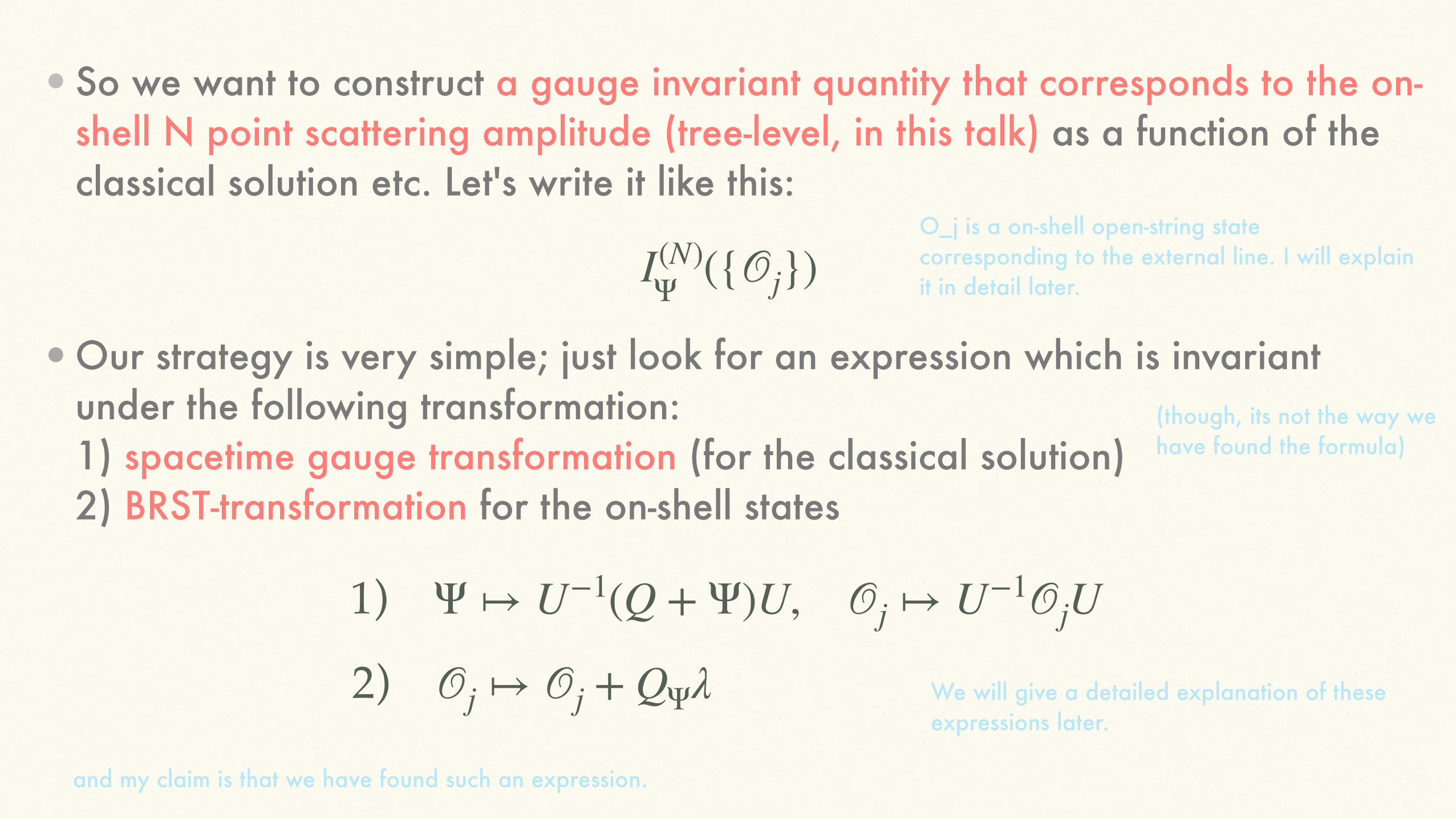
S[ΨT + Φ] = −1g2

o [ 12 ∫ ΦQTΦ +

13 ∫ ΦΦΦ] + energy(ΨT)

Tachyon vacuum solution(s)

QTϕ = Qϕ + ΨTϕ + ϕΨT

QT AT = 1

Physical excitation around the tachyon vacuum vanishes ⇔ existence of the homotopy operator

•Homotopy operator have been written down for most tachyon vacuum solutions.

Here we characterize the homotopy operator as an open string field of ghost number (-1). The 1 on the right side is the identity of the star product, which is also a string field.

To be precise, we need to consider the kernel of A_T, but let's not mind it here.

② Review of Witten’s open SFT etc۔

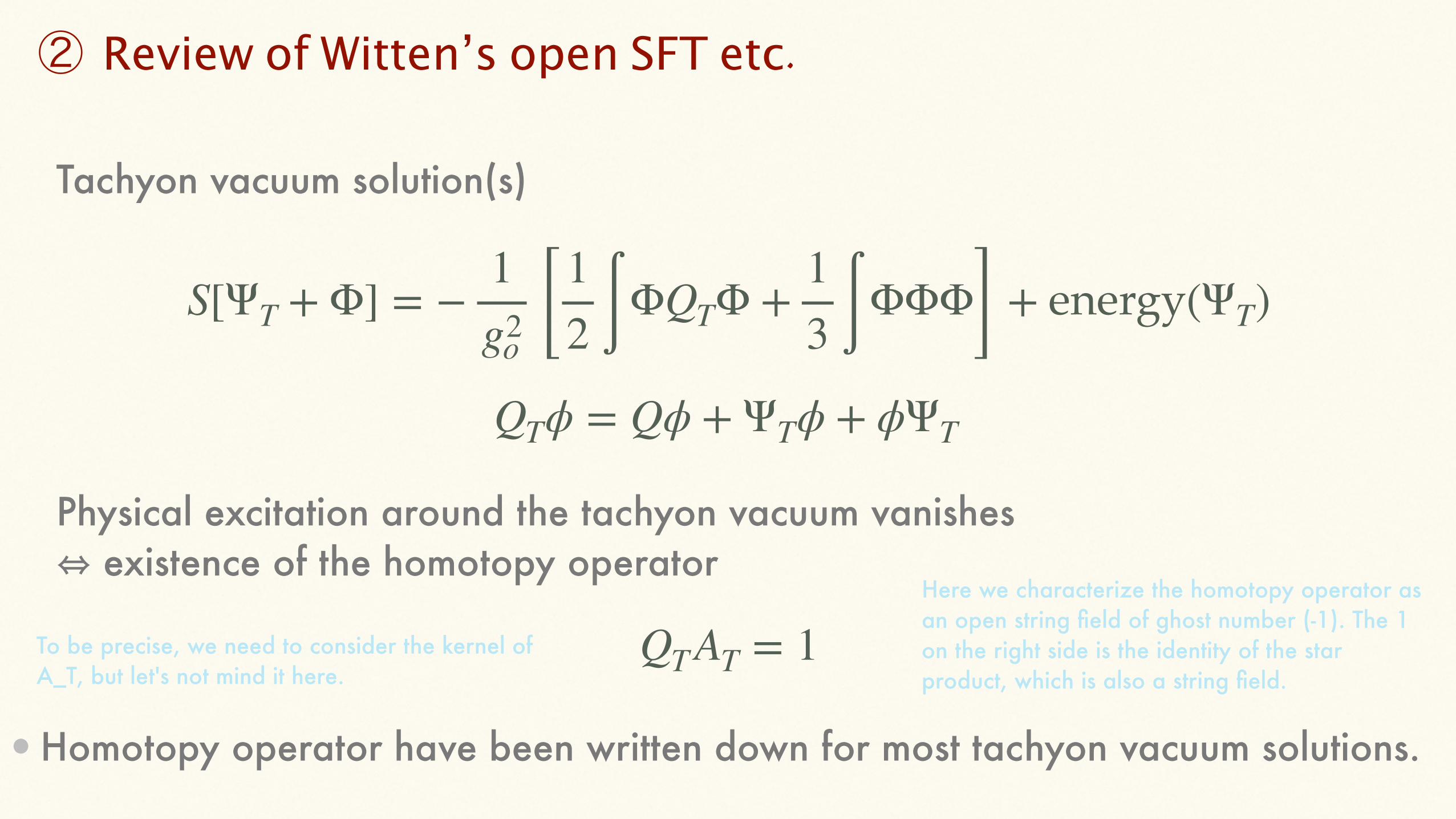
•The definition of the wedge state can be written concisely with the star product:

|n⟩ = |0⟩ * |0⟩ * . . . * |0⟩ ((n − 1) times)

•This can be generalized to non-negative real numbers.

|2⟩ = |0⟩ * |0⟩

•These algebraic relations are almost enough to define our gauge invariants. However, it is useful to prepare some technical tools to carry out concrete calculations as examples: wedge states, convenient coordinate systems, KBc algebra, etc.

② Review of Witten’s open SFT etc۔

It has already appeared in Martin's review, so it may not be necessary to be repeated here.

|0> on the right side is the conformal vacuum.|1⟩ = |0⟩

UHP Cπ : semi infinite cylinder

z = 2π arctan(ξ) ≡ f(ξ)

ξ

V(0) +1−1

z

f ∘ V(0)+1

16

|1⟩ |2⟩ = |1⟩ * |1⟩ |3⟩ = |1⟩ * |1⟩ * |1⟩ |x⟩

x321

eK e2K e3K exK

•K, B, c

K

x → 0

B

x → 0

eaK

a

c

x → 0

∫−i∞

i∞

dz2πi

b(z)∫−i∞

i∞

dz2πi

T(z)

c(0)

[K, B] = 0, {B, c} = 1,

•KBc algebra

QB = K, Qc = cKc

∫ cBex1Kcex2Kcex3Kcex4K = ∫dz2πi ⟨c(0)b(z)c(x1)c(x1 + x2)c(x1 + x2 + x3)⟩Cx1+x2+x3+x4

Relation with correlation functions on semi-infinite cylinders: an example

Cx1+x2+x3+x4

∫−i∞

i∞

dz2πi

b(z)

c(0) c(x1) c(x1 + x2) c(x1 + x2 + x3)

x1 + x2 + x3 + x4

•There are nice reviews on analytic solutions, KBc etc. （Fuchs-Kroyter 0807.4722; Schnabl 1004.4858; Okawa (2012) on PTEP;

original paper 0603159; T. Erler’s lecture note at school of the last SFT conference at HRI, etc..）

•The definition of KBc (more properly, the definition of star product) is roughly divided into two styles. (today we follow so-called Okawa’s convention)

If you're used to the other convention, what you care most in today's talk would be the sign of K. I think that there is no big influence except for it in today’s talk.

21

We use three fundamental quantities to define the gauge invariant quantity:

A𝒪j W

+1 ±０ −1

③ Definition of gauge invariant quantities for N = 3

QΨ𝒪j = 0

•We take the open string field of ghost number one, and impose the physical state condition around the classical solution:

•This object undergoes the following transformation under the gauge transformation of the classical solution:

𝒪j ↦ U𝒪jU−1

③ Definition of gauge invariant quantities for N = 3

•When considering a perturbative vacuum as a classical solution, you can typically choose the wedge state with an insertion of on-shell open string.

{Q, cV(x)} = 0

⇒ Q𝒪 = 0

•Sometimes it is useful to consider the limit, (the width) → 0.

𝒪

cV(O)

③ Definition of gauge invariant quantities for N = 3

•Definition of W

W = (Ψ − ΨT) * AT + AT * (Ψ − ΨT) = QΨAT − 1

QΨW = 0

•The important property is that W is Q_\Psi - closed,

•The change in W under replacement of tachyon vacuum solution is

W ↦ W + QΨ(UATU−1 − AT)

(if ΨT ↦ U(ΨT + Q)U−1)

③ Definition of gauge invariant quantities for N = 3

25

•As an example, take the Schnabl solution as a tachyon vacuum solution and the perturbative vacuum as a classical solution:

ΨT = eK2 c

KB1 − eK

ceK2

•In this case, W takes the following form.

W = eK

Namely, W is like a piece of the world sheet.

Ψ = 0

However, it is not necessary to remember the concrete form of the solution here. It is W that I will use later.

③ Definition of gauge invariant quantities for N = 3

•The boundary term is a formal object and can be characterized as follows:

•A is the homotopy operator of tachyon vacuum minus the “boundary term".

A = AT − (boundary term)

QΨA = W

•Such a quantity of course does not exist, but can be properly defined in correlation functions. Formally, the following relationship holds:

(boundary term) = AΨ, QΨAΨ = 1

③ Definition of gauge invariant quantities for N = 3

•As an example, let's consider again the case of choosing Schnabl solution as the tachyon vacuum solution and perturbative vacuum as the classical solution.

• In this case A is the following

A = ∫1

0dx exKB −

BK

So, A looks like a propagator (a half cut).

ΨT : Schnabl solution

Ψ = 0

③ Definition of gauge invariant quantities for N = 3

•BRST invariance: All of the objects are Q_\Psi closed, so the Q_\Psi exact part drops. Similarly, this quantity is invariant under replacement of the tachyon vacuum solution because the change of W is Q_\Psi exact.

I(3)Ψ = ∫ 𝒪1W𝒪2W𝒪3W

•Gauge invariance: a combination of (replacement of tachyon vacuum solution) and (gauge transformation) is just a similarity transformation, which preserves the Witten integral.

Definition for N=3

•Besides, this quantity is unchanged under replacement of the homotopy operator.

③ Definition of gauge invariant quantities for N = 3

29

•(Comment) you might have noticed that W’s in this definition are not necessary. and you might also find that you can insert any expression of W. That's correct, there are redundancy in this definition. I will comment on this point later again.

③ Definition of gauge invariant quantities for N = 3

•Let me skip the proof of gauge invariance, BRST invariance and other invariances. (you can check it from the definition.)

I(N)Ψ = C∑

σ∈S∫ (A + W)𝒪σ(1)(A + W)𝒪σ(2) . . . (A + W)𝒪σ(N)

•C is a simple combinatorial number (depending on the definition of the summation).

Definition for general N (>2)

④ Definition of gauge invariant quantities for general N

31

•(Comment) The following fact is important when checking gauge invariance.

∫ QΨ (expression including  1K ) ≠ 0

As (some of) you know, this is a common observation in study of multi-brane solutions in KBc (cf. Kojita-san’s talk). Although the construction of multi-brane solutions in this direction has not been done well, but part of experiences is useful in this way.

•Choose the Schnabl solution as a tachyon vacuum solution, and calculate the on-shell 4-point tachyon amplitude around the perturbative vacuum. As I mentioned earlier

W = eK

A = ∫1

0exKB −

exK

KB

x→0

main term boundary term

⑤ Example of calculation; 4 point tachyon amplitude

•For simplicity let's take the following O_j.

𝒪j

cV(0) = ceikj⋅X(0)

x → 0

cV(O)

(kj)2 =1α′�

⑤ Example of calculation; tachyon 4 point amplitude

•then the main term is given by

I(4)main({𝒪j}4

j=1) = C∑σ

∫ 𝒪σ(1)AT𝒪σ(1)W𝒪σ(1)W𝒪σ(1)W

This quantity can be written as follows after a change of the integration variable:

= C∑σ

∫1

0dx⟨𝒪σ(1)(0)𝒪σ(1)(x)𝒪σ(1)(x + 1)𝒪σ(1)(x + 2)⟩C3+x

= ∑{s,t,u}

∫12

0du u−α′�s−2(1 − u)−α′�t−2

⑤ Example of calculation; tachyon 4 point amplitude

∫ 𝒪1AT𝒪2W𝒪3W𝒪4W = ∫12

0du u...(1 − u)...

𝒪1 𝒪2 𝒪3 𝒪4

C3+x

𝒪1

𝒪2

x 1 1 1

Let us map the semi-infinite cylinder to a unit circle to get a sense of the range of integration. Let's follow the movement of the points.

𝒪3

𝒪4

W W WAT

⑤ Example of calculation; tachyon 4 point amplitude

36

W W

W

AT

𝒪1𝒪2

𝒪3

𝒪4

𝒪1

𝒪2

𝒪3

𝒪4

∫ 𝒪1AT𝒪2W𝒪3W𝒪4W = ∫12

0du u...(1 − u)...

x = 0

x = 1

at x = 0, O_1 and O_2 collide; at x = 1, O_2 is at the midpoint of O_1 and O_3. Of course, after mapping to the UHP, if you set O_1 to z = 0, O_3 to z = 1 and O_4 to x = infty, and O_2 will come to x = 1/2.

Collision

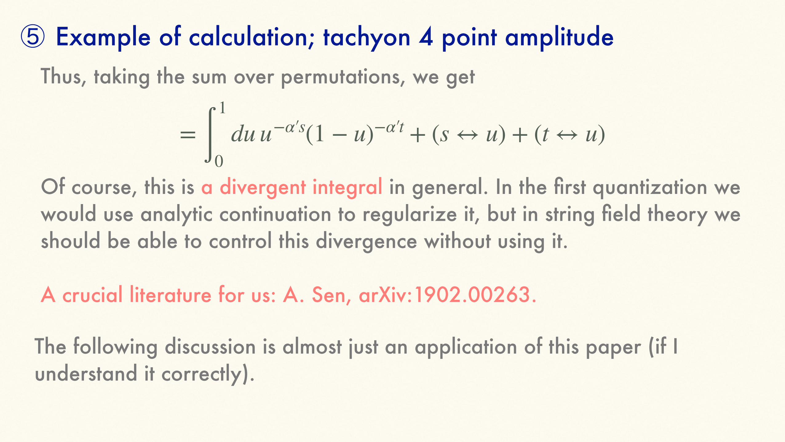
Of course, this is a divergent integral in general. In the first quantization we would use analytic continuation to regularize it, but in string field theory we should be able to control this divergence without using it. A crucial literature for us: A. Sen, arXiv:1902.00263.

= ∫1

0du u−α′�s(1 − u)−α′�t + (s ↔ u) + (t ↔ u)

The following discussion is almost just an application of this paper (if I understand it correctly).

Thus, taking the sum over permutations, we get

⑤ Example of calculation; tachyon 4 point amplitude

First, remember the following relation:

A = limϵ→0 ∫

1

ϵdx exKB −

exK

KB

x=ϵ= lim

ϵ→0 ∫1

ϵf1 − f0

x=ϵ

This relation should hold even after putting A into a correlation function and changing the integration variable from x to u.

df0 = f1

⑤ Example of calculation; tachyon 4 point amplitude

Therefore, the main term receives the following correction:

dg0(u) = u−α′�s−2(1 − u)−α′�t−2du

limϵ→0 ∫

12

ϵduu−α′�s−2(1 − u)−α′�t−2 + g0(u)

u=ϵ

Thus, at the limit of bringing ε to zero, we can choose:

g0(u) = ∑α<−1

Cα

α + 1uα+1, u−α′�s−2(1 − u)−α′�t−2 = ∑

α

Cαuα

⑤ Example of calculation; tachyon 4 point amplitude

C_\alpha is given by coefficients of the Laurant expansion of this function

This is nothing less than the minimal subtraction of the divergence of the main term. In this way, the Veneziano amplitude is reproduced without using an analytical continuation.

⑤ Example of calculation; tachyon 4 point amplitude

41

(Comment) If you select the Erler-Maccaferri solution as a classical solution

AΨ = ΣBK

Σ̄

Ψ = ΨT − ΣΨTΣ̄

In the correlation function, Σ’s cancel out altogether, and eventually reduces to the same formula as before.

W = ΣeKΣ̄ �̃�j = Σ𝒪jΣ̄

However, the physical state cannot be prepared unless the spectrum is known in advance.

⑤ Example of calculation; tachyon 4 point amplitude

•(It is related to what I just mentioned) we found a new formula, but in terms of application it can not be said that it is convenient enough. For example, can we calculate scattering amplitudes around classical solutions that are known only numerically ? It is not possible at present because it is difficult in the current technology to find a string field that satisfies the physical state condition around the classical solution.

④ Concluding comments

•Furthermore, it is desirable to make the formula simpler in order to perform numerical calculations.

•There are many generalizations or questions to be studied, but I don't think I have time to mention them. We are planning to have a list of problems in our paper.

•We might be able to regard our formula as one of the Feynman rule. Namely, it might be able to interpret the formula within the framework of a homological perturbation theory. Then, it would be possible to interpret the redundancy of the definition etc.

④ Concluding comments

この先にスライドはありません。