Beetle Bandit:

Evaluation of a Bayesian-adaptive reinforcement learning algorithm for bandit problemswith Bernoulli rewards.

A Thesis presented

by

Bart Jan Buter

in partial ful�llment of the requirements

for the degree of

Bachelor of Science in Arti�cial Intelligence

Bachelor's programme in Arti�cial Intelligence

Faculty of ScienceUniversiteit van Amsterdam

The NetherlandsJune 2006

Dedicated toMom and Dad

for their ongoing displayof unconditional love.

ii

Beetle Bandit

Bart J. Buter

Submitted for the degree of

Bachelor of Science in Arti�cial IntelligenceJune 2006

Abstract

A novel approach to Bayesian Reinforcement learning (RL) named Beetle has recently been pre-sented; this approach nicely balances exploration vs. exploitation while learning is performedonline. This has produced an interest into experimental results obtained from the Beetle algo-rithm. This thesis gives an overview of bandit problems and modi�es the Beetle algorithm. Thenew Beetle Bandit algorithm is applied to the multi-armed bandit class of problems, therebycomparing the resulting Beetle Bandit algorithm with traditional and current Bayesian inspiredapproaches.

iii

Declaration

The work in this thesis is based on research carried out at the Faculty of Science of the Universiteitvan Amsterdam The Netherlands. No part of this thesis has been submitted elsewhere for anyother degree or quali�cation and it all my own work performed under the guidance of my projectsupervisor unless referenced to the contrary in the text.

Copyright c© 2006 by Bart J. Buter.

�The copyright of this thesis rests with the author. No quotations from it should be publishedwithout the author's prior written consent and information derived from it should be acknowl-edged�.

iv

Acknowledgments

Nikos Vlassis for his inspiring courses and his guidance during this �nal bachelor's project.My mentor Leo Dorst for his guidance and advice during my bachelors programme, though westill have to really drink co�ee some day. All teachers of the courses I have taken during mybachelors programme. My fellow students for our pleasant co-operation and indulging classes.Radboud Winkels and Frits de Vries for giving me the opportunity to be student assistant fortheir courses. Friends and family for their many proof-readings and general support during myeducation. Especially, sis for taking care of your little brother as you so often do. Dad for hisongoing support, insight and guidance, and Mom though your mind may be leaving your spiritnever has.

Thank you all.

v

Contents

Abstract iii

Declaration iv

Acknowledgements v

1 Introduction 1

1.1 Introduction . . . . . . . . . . . . . . . . . . . . . . . . . . . . . . . . . . . . . . . 11.2 Layman's overview . . . . . . . . . . . . . . . . . . . . . . . . . . . . . . . . . . . 21.3 Problem description . . . . . . . . . . . . . . . . . . . . . . . . . . . . . . . . . . 3

2 Bandits Problems 4

2.1 Historical Background . . . . . . . . . . . . . . . . . . . . . . . . . . . . . . . . . 42.2 Problem Statement . . . . . . . . . . . . . . . . . . . . . . . . . . . . . . . . . . 42.3 Important Concepts . . . . . . . . . . . . . . . . . . . . . . . . . . . . . . . . . . 5

2.3.1 Gittins Index . . . . . . . . . . . . . . . . . . . . . . . . . . . . . . . . . . 52.3.2 Lai and Robbins . . . . . . . . . . . . . . . . . . . . . . . . . . . . . . . . 6

2.4 The Bandit problem as MDPs . . . . . . . . . . . . . . . . . . . . . . . . . . . . . 62.4.1 Bandits as a Markov decision process . . . . . . . . . . . . . . . . . . . . . 62.4.2 Bandits as POMDP or BAMDP . . . . . . . . . . . . . . . . . . . . . . . 7

2.5 Beetle Bandit . . . . . . . . . . . . . . . . . . . . . . . . . . . . . . . . . . . . . . 82.5.1 The Bellman Equation . . . . . . . . . . . . . . . . . . . . . . . . . . . . . 82.5.2 Value functions . . . . . . . . . . . . . . . . . . . . . . . . . . . . . . . . . 9

2.6 Beetle Bandit Algorithm . . . . . . . . . . . . . . . . . . . . . . . . . . . . . . . . 92.7 Beetle Bandit-2 and other improvements . . . . . . . . . . . . . . . . . . . . . . 10

3 Previous approaches 11

3.1 ε-Greedy algorithms . . . . . . . . . . . . . . . . . . . . . . . . . . . . . . . . . . 113.1.1 basic ε-greedy . . . . . . . . . . . . . . . . . . . . . . . . . . . . . . . . . . 113.1.2 ε-�rst . . . . . . . . . . . . . . . . . . . . . . . . . . . . . . . . . . . . . . 113.1.3 ε-decreasing . . . . . . . . . . . . . . . . . . . . . . . . . . . . . . . . . . . 123.1.4 LeastTaken . . . . . . . . . . . . . . . . . . . . . . . . . . . . . . . . . . . 12

3.2 Softmax algorithms . . . . . . . . . . . . . . . . . . . . . . . . . . . . . . . . . . . 123.2.1 Gibbs-Softmax . . . . . . . . . . . . . . . . . . . . . . . . . . . . . . . . . 123.2.2 Softmix . . . . . . . . . . . . . . . . . . . . . . . . . . . . . . . . . . . . . 123.2.3 Exp3 . . . . . . . . . . . . . . . . . . . . . . . . . . . . . . . . . . . . . . . 12

3.3 Interval estimation . . . . . . . . . . . . . . . . . . . . . . . . . . . . . . . . . . . 133.4 Poker . . . . . . . . . . . . . . . . . . . . . . . . . . . . . . . . . . . . . . . . . . 133.5 UCB2 . . . . . . . . . . . . . . . . . . . . . . . . . . . . . . . . . . . . . . . . . . 143.6 Optimistically initialized Greedy . . . . . . . . . . . . . . . . . . . . . . . . . . . 14

vi

Contents vii

4 Experiments 15

4.1 Overview of experimental setup . . . . . . . . . . . . . . . . . . . . . . . . . . . . 154.2 2-Armed bandit experiments . . . . . . . . . . . . . . . . . . . . . . . . . . . . . . 15

4.2.1 Experimental setup . . . . . . . . . . . . . . . . . . . . . . . . . . . . . . . 154.2.2 Discussion of results 2-armed Bandit experiments . . . . . . . . . . . . . . 16

4.3 5-Armed Beetle experiment . . . . . . . . . . . . . . . . . . . . . . . . . . . . . . 164.3.1 Experimental setup . . . . . . . . . . . . . . . . . . . . . . . . . . . . . . . 164.3.2 Discussion of results 5-armed Bandit experiments . . . . . . . . . . . . . . 17

5 Conclusion 18

List of Tables

4.1 Best average rewards and regrets per round for 2-armed Bandit . . . . . . . . . . 164.2 Results by Wang et al. compared with Beetle Bandit, 5-armed bandit reward per

round is reported . . . . . . . . . . . . . . . . . . . . . . . . . . . . . . . . . . . . 17

viii

Chapter 1

Introduction

1.1 Introduction

Reinforcement learning (RL) is presented as a �eld especially suited for problems where plan-ning and learning has to take place simultaneously. A common theme in these problems is theexploration-exploitation trade-o�; is it best to exploit the knowledge obtained or do you exploreto increase the knowledge base? A prevalent solution to this trade-o� is amortization of the costof exploring, leading to asymptotically optimal behavior, see [17] for a variety of these algorithms.

Bayesian approaches to RL o�er the prospect of optimal behavior because an informed trade-o� can be made between the cost of obtaining new information and the future reward exploitationthis new information will likely provide. This is achieved by learning a transition-reward model,a prior distribution is de�ned over transition and reward models, the prior distribution and newobservation are used to determine the posterior distribution, that is the updated transition-reward model. A drawback of the Bayesian approach to RL has been the intractability of theseapproaches.

However, recent developments have made approximate solutions to partially observable Markovdecision processes (POMDPs) tractable. This, coupled with the knowledge that Bayesian adap-tive Markov decision processes (BAMDPs) can be modeled as POMDPs [8], has created a renewedinterest in Bayesian approaches. One of the results of this renewed interest is Beetle (BayesianExploration Exploitation Trade-o� in LEarning) [14].

Multi-armed bandit problems are prototypical problems which display the exploration- ex-ploitation trade-o�. These bandit problems are �rst described by Robbins [15]. In these problemsan agent gets to pull one of multiple levers connected to a slot-machine and every lever payso� according to an underlying unknown probability distribution. The objective is to gain max-imum reward by pulling the levers, or, more common in this setting, minimizing regret, whichis the amount of possible reward lost because of pulling a sub-optimal lever. The exploration-exploitation trade-o� now becomes a question of pulling the lever with the highest payo� so farversus pulling a sub-optimal lever but gaining more certainty on the underlying distributions.

This thesis is the result of a four week project, which completes the quali�cations neededin obtaining the Bachelor of Science degree in Arti�cial Intelligence. The project is aimed atevaluating the Beetle algorithm in the multi-armed bandit setting. This thesis is organized asfollows: Chapter 1 will give a layman's overview aimed towards friends and family, then it willgive a description of the project and its setup. Chapter 2 is aimed to give a literature overviewon bandit problems in the �eld of reinforcement learning and it will give insight into the BeetleBandit algorithm. Chapter 3 will describe algorithms used in the comparison of the new BeetleBandit algorithm. Chapter 4 will describe experimental results. Chapter 5 will give a conclusionto this project and give ideas for possible future research.

1

1.2. Layman's overview 2

1.2 Layman's overview

Suppose you enter a casino and the manager welcomes you as the one millionth visitor. Of course,this means you win a special prize. You are let into a room with a few di�erent slot machines.You are allowed to play these one-armed bandits for free, for a �xed period, wanting to extractas much money as quickly as possible from the machines. How will you be able to achieve thisgoal? By playing the machines you have to �nd out which machine on average pays out themost and then play this best paying machine, while minimizing the plays on the machine thatpays out the least. The problem you are faced with is a classical dilemma between explorationand exploitation. In this case the exploration means playing the machine which has, so far, onaverage given less payout, but by playing it you are gaining more knowledge and con�dence thatthis machine is worse. Exploiting means playing the machine that has shown the best averagepayout until now, but how can you be sure this is indeed the best machine to play?

Robbins [15] came up with this multi-armed bandit problem to investigate the exploration-exploitation trade-o�. These problems were �rst studied as statistical problems; however, withthe advent of computing it is being studied in computer science. Reinforcement learning (RL) isa machine learning setting where an agent learns a policy (how to behave) by receiving positive ornegative rewards while interacting with the environment. This setting is well suited for the banditproblem because both deal with actions and subsequent rewards. This thesis investigates thebandit problem in a RL setting and presents results for di�erent algorithms, one of which is ournew Beetle bandit algorithm, playing the multi-armed bandit. More speci�cally, it investigatesthe problem where a choice has to be made between machines which pay out 0 or 1 each time,but on average pay a �xed amount per play.

An intuitive way of dealing with this problem is keeping an estimate of the payout probability,thus an average for every machine, and updating this estimate every time a machine is playedand more information about the real probability is received. This estimate will be called a belief;with all the information we have received until now we believe the underlying probability to beour estimate. Updating beliefs in the light of new evidence can mathematically be done withBayes' theorem.

However, this �rst intuitive solution loses the notion of certainty about your belief. Forexample observing an average of 0.8 for arm 2 over 100 plays gives more certainty of what is tobe expected next time arm 2 is pulled than observing the same average over 10 plays. This iswhy we take our belief to be a probability distribution over our estimate, meaning we do notsay we believe the real probability for arm 2 is 0.8, but we now say we think 0.8 is the mostprobable real probability. The real probability might also be 0.5, but this is less likely, though0.5 is more likely with 10 observations than with 100. We can now make an informed decisionbetween gaining short term rewards and/or improving the certainty of our estimates. This newapproach, however, causes computational problems.

Since our beliefs are no longer a �xed set of averages but all possible distributions, we cannotcompute the best actions to take but we have to make due with estimates. Previous Bayesianapproaches to RL slowly computed the estimates online ("while playing") a game. They aretherefore impractical in real life applications, For example when a router has to choose the bestpeer to send a packet it has to be able to decide in milliseconds. However, if this router couldpre-compute intermediate results o�ine (before it is brought into service) it could provide fastonline service.

Due to certain mathematical properties of the bandit problem which will be derived in thisthesis, we are capable of such a fast online algorithm. We do this by �rst imagining that weare playing multi-armed bandit problems and then pre-computing the belief updates; playingthe game has now become considerably less intensive computationally for the online decisionmaking.

Poupart et al. [14] have recently described a new algorithm from which the new Beetle Banditalgorithm is derived. Beetle is capable of making a good trade-o� between exploration and

1.3. Problem description 3

exploitation while still making fast online decisions. There is a demand for experimental resultsfrom this algorithm. This is why it has been adapted for the multi-armed bandit problem. Wehave compared it to several other algorithms and found that the new Beetle Bandit algorithmperforms equal to, if not better than, any of the other reviewed classical algorithms, as longas the problem is kept small. For larger problems other algorithms such as Wang's samplingmethods [20] have been found to be better.

1.3 Problem description

The project has primarily been setup to gain experimental data on the Beetle algorithm; morespeci�cally, we have chosen to gather experimental data in order to compare the Beetle algorithmwith existing algorithms. The project aims are three-fold:

• Adapting the Beetle algorithm to the domain of bandit problems.

• Review literature on bandit problems to see how this new algorithm compares to existingapproaches.

• Gather experimental results to compare Beetle Bandit with algorithms found in literature.

Chapter 2

Bandits Problems

2.1 Historical Background

Bandit problems are a prototypical example of the exploration-exploitation trade-o� seen inmachine learning algorithms in general and reinforcement learning in particular. The problemwas �rst proposed by Robbins [15]. Put simply, a slot machine with multiple arms, all withdi�erent payo� probabilities, can be played with the aim of maximizing reward. There havebeen many variations on this basic bandit problem. For instance, Du� [7] attaches a rewardprocess to each arm where the reward is dependent on the arm chosen and the internal state ofthe process attached to this arm. Cicirello et al. [5] try to maximize the largest single reward,while Hardwick et al. [12] study a bandit problem with delayed reward signal. This variety inbandit problems is due to the simplicity, complexity and universality of the problem. That is,the problem statement is easy to grasp and understand, yet it manifests all complexity of theexploration-exploitation trade-o�. This is why it has found it's way from sequential design instatistics into machine learning [1], and in particular, reinforcement learning [17] and practicalapplications such as clinical trial design [11].

Three works are of particular importance to the �eld of bandit problems, namely those byBellman [3], Gittins and Jones [10] and Lai and Robbins [13]. Bellman proved that the optimalBayesian solution was intractable. Gittins and Jones' paper is often described as making theproblem tractable. They prove that the optimal decision can be found by computing an index,independent of other arms, for every separate arm after which the optimal choice is the arm withthe highest index. However, the computation of the indices is not trivial and needs informationabout the reward processes [1]. Lai and Robbins proved that optimal exploration policies can beachieved where the regret grows logarithmically with respect to the horizon of the problem.

2.2 Problem Statement

The basic bandit problem is well stated by Auer et al. [1], which we will follow closely in theproblem description of the multi-armed bandit with Bernoulli distributed rewards.

A K-armed bandit problem is de�ned by random variables Xi,m for 1 ≤ a ≤ K and m ≥ 1, where m denotes time and a is the index of an arm or lever of the bandit. By playing the K-armed bandits ath arm rewards Xa,1, Xa,2, ... are received, these are independent and identicallydistributed according to the Bernoulli distribution with unknown expectation µa. This meansPr(Xa,m = 1) = µa where 0 ≤ µa ≤ 1. The rewards across arms are also independent; that isXa,s and Xb,t are independent for each 1 ≤ a ≤ b ≤ K and each s, t≥ 1.

A policy, or allocation strategy, A is an algorithm that chooses the action to take, thuswhich arm to pull, based on the previous plays and subsequent obtained rewards. Let Xa,mbethe reward received when arm a was pulled at time m. Then the regret of A after m plays isde�ned by

4

2.3. Important Concepts 5

µ?m−m∑

t=1

E[Xπt,t] (2.1)

whereµ? = max

1≤a≤Kµa (2.2)

and E[·] denotes expectation, πt, denotes the action taken at time t when following policy π.Thus the regret is the expected loss due to the fact that the policy does not always play the bestarm.

A division can be made between problems with �nite vs. in�nite horizons. Bandit problemswith �nite horizons stop after a certain number of rounds, whereas the in�nite horizon problemsnever stop. A consequence of the in�nite problem setting is that future cumulative rewardalso becomes in�nite. This is why future cumulative rewards for in�nite problems need to bediscounted by a term 0 < γ < 1, cumulative future reward then becomes

R =∞∑

m=1

γm−1rm (2.3)

where rm is the reward received at time m. For �nite horizon problems the discount factor γ = 1can be used to cancel discounting. Since regret is related to reward, future cumulative regretalso has to be discounted.

2.3 Important Concepts

Two concepts are of particular importance to Bandit problems, the Gittins index and the proofby Lai and Robins about �optimal" regret, both will be discussed in this section. It is importantto note that both concepts are about the in�nite bandit case, the Gittins index needs in�nitecumulative rewards, while Lai and Robbins claims hold when m →∞

2.3.1 Gittins Index

This section will describe and give an intuition into the so called Gittins index [9, 10].Suppose we have a 1-armed bandit with rewards drawn from an unknown Bernoulli distribu-

tion. Let na denote the number of times a positive reward of 1 is observed after pulling arm aand na, denotes the number of times a reward of 0 has been observed after pulling a, and let γbe a discount factor where 0 < γ < 0. We can now express a value function that is dependenton observations of rewards in the following way

V (n, n) =n

n + n[1 + γV (n + 1, n)] +

n

n + nγV (n, n + 1) (2.4)

This means we multiply the the chance of receiving a reward rm ∈ {0, 1}, by the obtained rewardand all future rewards for both the reward 0 and 1. The future rewards are expressed as a valuefunction with updated observations. This is a Bayesian approach, because the prior probabilityis used to update the posterior probability with the newly observed rewards.

Suppose we now add an arm to this bandit which gives reward 1 with probability p, thisprobability is known to the player of the bandit. The discounted reward at round m will thenbe γm−1rm and the in�nite cumulative reward is given by equation 2.3, for a �xed reward r thiswill be r

1−γ . The new value function for this problem becomes

V (n, n) = max{

p

1− γ,

n

n + n[1 + γV (n + 1, n)] +

n

n + nγV (n, n + 1)

}(2.5)

2.4. The Bandit problem as MDPs 6

The new formula expresses that a choice has to be made between pulling the new arm with�xed probability p or the arm with unknown probability. The Gittins index is de�ned as the pwhere the value of pulling the arm with unknown probability is equal to the one with knownprobability.

For a multi-armed bandit the best action is to pull the arm with the highest Gittins index.However, the Gittins index is not easy to compute, it can be solved iteratively, but this is not atrivial computation.

2.3.2 Lai and Robbins

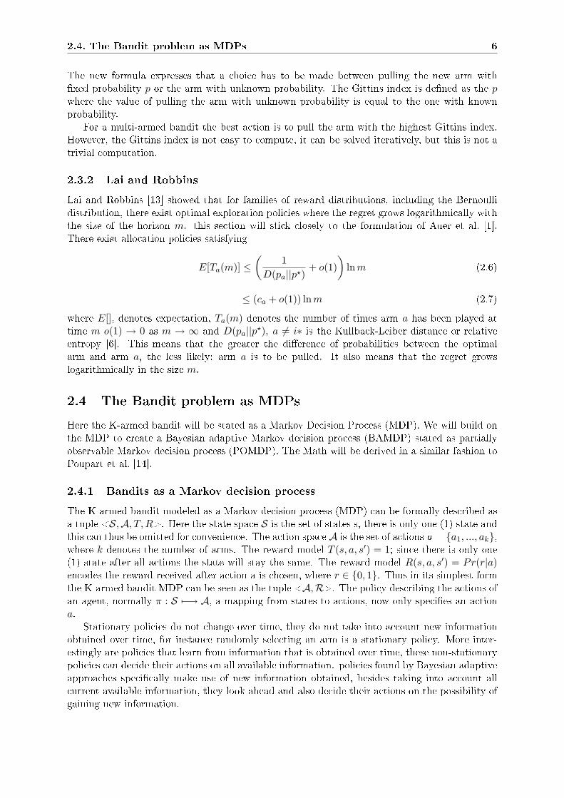
Lai and Robbins [13] showed that for families of reward distributions, including the Bernoullidistribution, there exist optimal exploration policies where the regret grows logarithmically withthe size of the horizon m. this section will stick closely to the formulation of Auer et al. [1].There exist allocation policies satisfying

E[Ta(m)] ≤(

1D(pa||p?)

+ o(1))

lnm (2.6)

≤ (ca + o(1)) lnm (2.7)

where E[], denotes expectation, Ta(m) denotes the number of times arm a has been played attime m o(1) → 0 as m → ∞ and D(pa||p?), a 6= i∗ is the Kullback-Leiber distance or relativeentropy [6]. This means that the greater the di�erence of probabilities between the optimalarm and arm a, the less likely; arm a is to be pulled. It also means that the regret growslogarithmically in the size m.

2.4 The Bandit problem as MDPs

Here the K-armed bandit will be stated as a Markov Decision Process (MDP). We will build onthe MDP to create a Bayesian adaptive Markov decision process (BAMDP) stated as partiallyobservable Markov decision process (POMDP). The Math will be derived in a similar fashion toPoupart et al. [14].

2.4.1 Bandits as a Markov decision process

The K-armed bandit modeled as a Markov decision process (MDP) can be formally described asa tuple <S,A, T, R>. Here the state space S is the set of states s, there is only one (1) state andthis can thus be omitted for convenience. The action space A is the set of actions a = {a1, ..., ak},where k denotes the number of arms. The reward model T (s, a, s′) = 1; since there is only one(1) state after all actions the state will stay the same. The reward model R(s, a, s′) = Pr(r|a)encodes the reward received after action a is chosen, where r ∈ {0, 1}. Thus in its simplest formthe K-armed bandit MDP can be seen as the tuple <A,R>. The policy describing the actions ofan agent, normally π : S 7−→ A, a mapping from states to actions, now only speci�es an actiona.

Stationary policies do not change over time, they do not take into account new informationobtained over time, for instance randomly selecting an arm is a stationary policy. More inter-estingly are policies that learn from information that is obtained over time, these non-stationarypolicies can decide their actions on all available information. policies found by Bayesian adaptiveapproaches speci�cally make use of new information obtained, besides taking into account allcurrent available information, they look ahead and also decide their actions on the possibility ofgaining new information.

2.4. The Bandit problem as MDPs 7

2.4.2 Bandits as POMDP or BAMDP

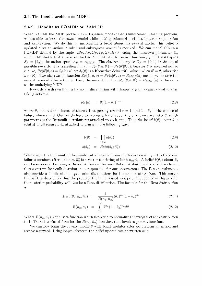
When we cast the MDP problem as a Bayesian model-based reinforcement learning problem,we are able to learn the reward model while making informed decisions between exploitationand exploration. We do this by introducing a belief about the reward model; this belief isupdated after an action is taken and subsequent reward is received. We can model this as aPOMDP de�ned by the tuple <SP ,AP ,OP , TP , ZP , RP>, using the unknown parameter θa,which describes the parameter of the Bernoulli distributed reward function µa. The state spaceSP = {θa}, the action space AP = AMDP . The observation space OP = {0, 1} is the set ofpossible rewards. The transition function TP (θ, a, θ′) = Pr(θ′|θ, a), because θ is assumed not tochange, Pr(θ′|θ, a) = δθ(θ′) where δθ(θ) is a Kronecker delta with value 1 when θ′ = θ, otherwisezero (0). The observation function ZP (θ′, a, o) = Pr(o|θ′, a) = RMDP (a) means we observe thereward received after action a. Last, the reward function RP (θ, a, θ′) = RMDP (a) is the sameas the underlying MDP.

Rewards are drawn from a Bernoulli distribution with chance of p to obtain reward r, aftertaking action a

p(r|a) = θra(1− θa)1−r (2.8)

where θa denotes the chance of success thus getting reward r = 1, and 1 − θa is the chance offailure where r = 0. Our beliefs have to express a belief about the unknown parameter θ, whichparametrizes the Bernoulli distributions attached to each arm. Thus the belief b(θ) about θ isrelated to all separate θa attached to arm a in the following way.

b(θ) =∏a∈A

b(θa) (2.9)

b(θa) = Beta(θa;−→na) (2.10)

Where na− 1 is the count of the number of successes obtained after action a, na− 1 is the countfailures obtained after action a, −→na is a vector consisting of both na, na. A belief b(θa) about θa

can be expressed by using a Beta distribution, because Beta distributions describe the chancethat a certain Bernoulli distribution is responsible for our observations. The Beta distributionsalso provide a family of conjugate prior distributions for Bernoulli distributions. This meansthat a Beta distribution has the property that if it is used as a prior probability in Bayes' rule,the posterior probability will also be a Beta distribution. The formula for the Beta distributionis

Beta(θa;na, na) =1

B(na, na)(θa)na(1− θa)na (2.11)

B(na, na) =∫ 1

0θna(1− θa)nadθ (2.12)

Where B(na, na) is the Beta function which is needed to normalize the integral of the distributionto 1. There is a closed form for the B(na, na) function, that involves gamma functions.

We can now learn the reward model θ with belief updates after we perform an action andreceive a reward. Using Bayes' theorem the belief update can be written as :

2.5. Beetle Bandit 8

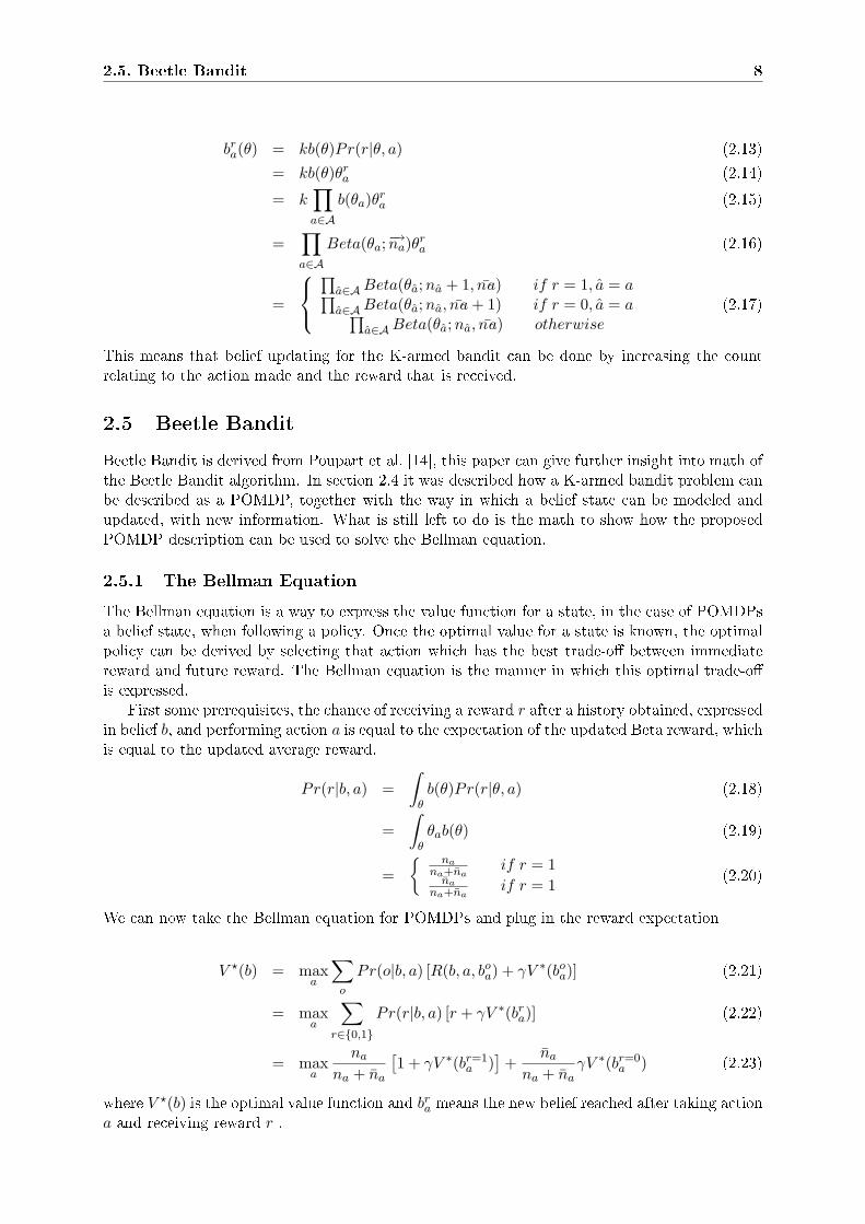
bra(θ) = kb(θ)Pr(r|θ, a) (2.13)

= kb(θ)θra (2.14)

= k∏a∈A

b(θa)θra (2.15)

=∏a∈A

Beta(θa;−→na)θra (2.16)

=

∏

a∈A Beta(θa;na + 1, na) if r = 1, a = a∏a∈A Beta(θa;na, na + 1) if r = 0, a = a∏

a∈A Beta(θa;na, na) otherwise(2.17)

This means that belief updating for the K-armed bandit can be done by increasing the countrelating to the action made and the reward that is received.

2.5 Beetle Bandit

Beetle Bandit is derived from Poupart et al. [14], this paper can give further insight into math ofthe Beetle Bandit algorithm. In section 2.4 it was described how a K-armed bandit problem canbe described as a POMDP, together with the way in which a belief state can be modeled andupdated, with new information. What is still left to do is the math to show how the proposedPOMDP description can be used to solve the Bellman equation.

2.5.1 The Bellman Equation

The Bellman equation is a way to express the value function for a state, in the case of POMDPsa belief state, when following a policy. Once the optimal value for a state is known, the optimalpolicy can be derived by selecting that action which has the best trade-o� between immediatereward and future reward. The Bellman equation is the manner in which this optimal trade-o�is expressed.

First some prerequisites, the chance of receiving a reward r after a history obtained, expressedin belief b, and performing action a is equal to the expectation of the updated Beta reward, whichis equal to the updated average reward.

Pr(r|b, a) =∫

θb(θ)Pr(r|θ, a) (2.18)

=∫

θθab(θ) (2.19)

={ na

na+naif r = 1

nana+na

if r = 1(2.20)

We can now take the Bellman equation for POMDPs and plug in the reward expectation

V ?(b) = maxa

∑o

Pr(o|b, a) [R(b, a, boa) + γV ∗(bo

a)] (2.21)

= maxa

∑r∈{0,1}

Pr(r|b, a) [r + γV ∗(bra)] (2.22)

= maxa

na

na + na

[1 + γV ∗(br=1

a )]+

na

na + naγV ∗(br=0

a ) (2.23)

where V ?(b) is the optimal value function and bra means the new belief reached after taking action

a and receiving reward r .

2.6. Beetle Bandit Algorithm 9

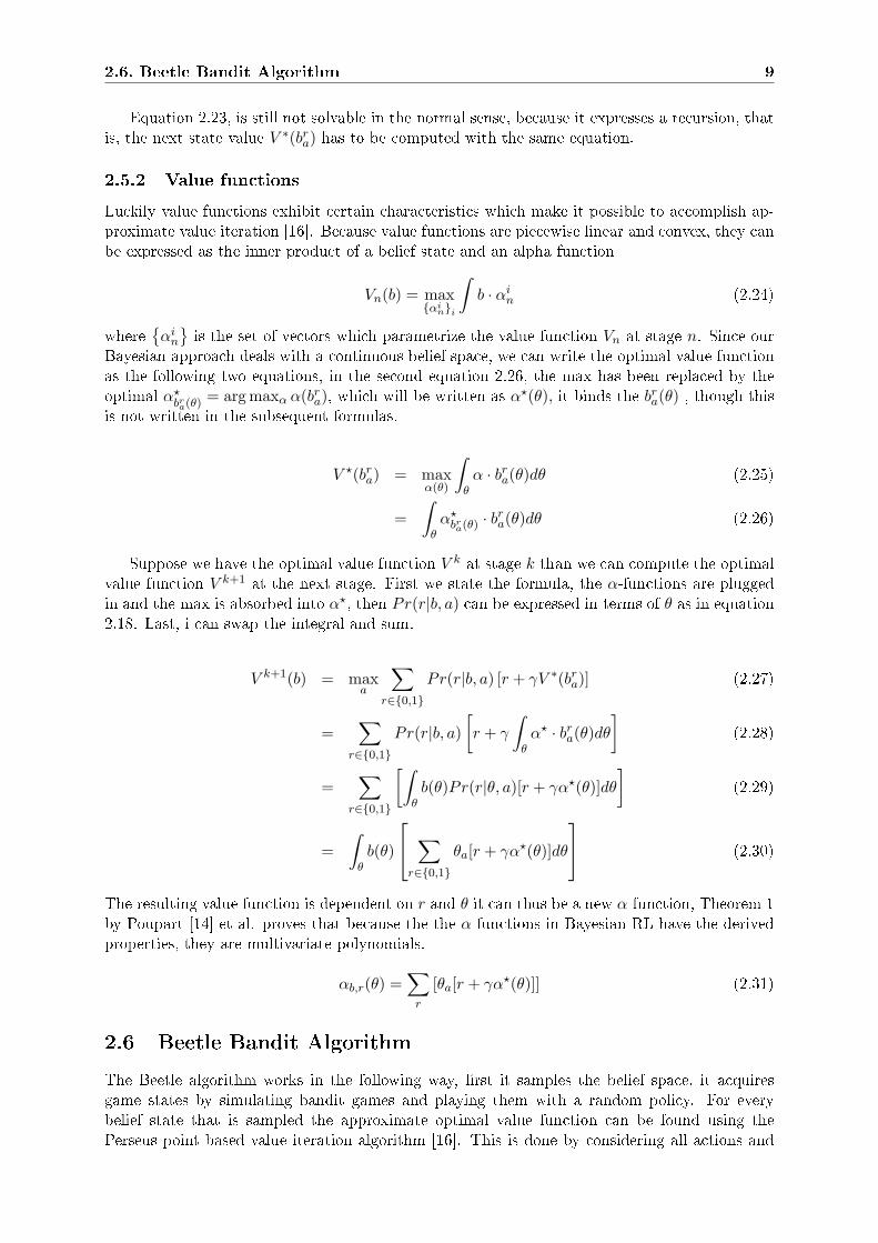
Equation 2.23, is still not solvable in the normal sense, because it expresses a recursion, thatis, the next state value V ∗(br

a) has to be computed with the same equation.

2.5.2 Value functions

Luckily value functions exhibit certain characteristics which make it possible to accomplish ap-proximate value iteration [16]. Because value functions are piecewise linear and convex, they canbe expressed as the inner product of a belief state and an alpha function

Vn(b) = max{αi

n}i

∫b · αi

n (2.24)

where{αi

n

}is the set of vectors which parametrize the value function Vn at stage n. Since our

Bayesian approach deals with a continuous belief space, we can write the optimal value functionas the following two equations, in the second equation 2.26, the max has been replaced by theoptimal α?

bra(θ) = arg maxα α(br

a), which will be written as α?(θ), it binds the bra(θ) , though this

is not written in the subsequent formulas.

V ?(bra) = max

α(θ)

∫θα · br

a(θ)dθ (2.25)

=∫

θα?

bra(θ) · b

ra(θ)dθ (2.26)

Suppose we have the optimal value function V k at stage k than we can compute the optimalvalue function V k+1 at the next stage. First we state the formula, the α-functions are pluggedin and the max is absorbed into α?, then Pr(r|b, a) can be expressed in terms of θ as in equation2.18. Last, i can swap the integral and sum.

V k+1(b) = maxa

∑r∈{0,1}

Pr(r|b, a) [r + γV ∗(bra)] (2.27)

=∑

r∈{0,1}

Pr(r|b, a)[r + γ

∫θα? · br

a(θ)dθ

](2.28)

=∑

r∈{0,1}

[∫θb(θ)Pr(r|θ, a)[r + γα?(θ)]dθ

](2.29)

=∫

θb(θ)

∑r∈{0,1}

θa[r + γα?(θ)]dθ

(2.30)

The resulting value function is dependent on r and θ it can thus be a new α-function, Theorem 1by Poupart [14] et al. proves that because the the α-functions in Bayesian RL have the derivedproperties, they are multivariate polynomials.

αb,r(θ) =∑

r

[θa[r + γα?(θ)]] (2.31)

2.6 Beetle Bandit Algorithm

The Beetle algorithm works in the following way, �rst it samples the belief space, it acquiresgame states by simulating bandit games and playing them with a random policy. For everybelief state that is sampled the approximate optimal value function can be found using thePerseus point based value iteration algorithm [16]. This is done by considering all actions and

2.7. Beetle Bandit-2 and other improvements 10

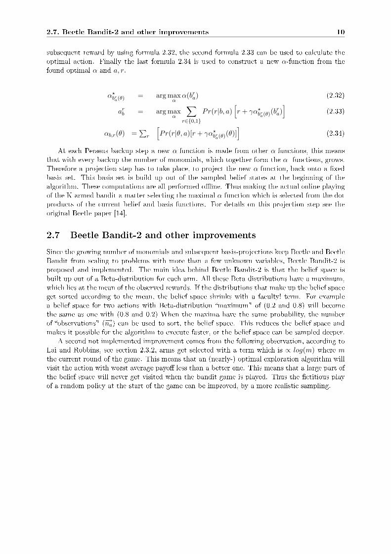
subsequent reward by using formula 2.32, the second formula 2.33 can be used to calculate theoptimal action. Finally the last formula 2.34 is used to construct a new α-function from thefound optimal α and a, r.

α?bra(θ) = arg max

αα(br

a) (2.32)

arb = arg max

α

∑r∈{0,1}

Pr(r|b, a)[r + γα?

bra(θ)(b

ra)

](2.33)

αb,r(θ) =∑

r

[Pr(r|θ, a)[r + γα?

bra(θ)(θ)]

](2.34)

At each Perseus backup step a new α-function is made from other α-functions, this meansthat with every backup the number of monomials, which together form the α -functions, grows.Therefore a projection step has to take place, to project the new α-function, back onto a �xedbasis set. This basis set is build up out of the sampled belief states at the beginning of thealgorithm. These computations are all performed o�ine. Thus making the actual online playingof the K-armed bandit a matter selecting the maximal α-function which is selected from the dotproducts of the current belief and basis functions. For details on this projection step see theoriginal Beetle paper [14].

2.7 Beetle Bandit-2 and other improvements

Since the growing number of monomials and subsequent basis-projections keep Beetle and BeetleBandit from scaling to problems with more than a few unknown variables, Beetle Bandit-2 isproposed and implemented. The main idea behind Beetle Bandit-2 is that the belief space isbuilt up out of a Beta-distribution for each arm. All these Beta distributions have a maximum,which lies at the mean of the observed rewards. If the distributions that make up the belief spaceget sorted according to the mean, the belief space shrinks with a faculty! term. For examplea belief space for two actions with Beta-distribution �maximum" of (0.2 and 0.8) will becomethe same as one with (0.8 and 0.2) When the maxima have the same probability, the numberof �observations" (−→na) can be used to sort, the belief space. This reduces the belief space andmakes it possible for the algorithm to execute faster, or the belief space can be sampled deeper.

A second not implemented improvement comes from the following observation, according toLai and Robbins, see section 2.3.2, arms get selected with a term which is ∝ log(m) where mthe current round of the game. This means that an (nearly-) optimal exploration algorithm willvisit the action with worst average payo� less than a better one. This means that a large part ofthe belief space will never get visited when the bandit game is played. Thus the �ctitious playof a random policy at the start of the game can be improved, by a more realistic sampling.

Chapter 3

Previous approaches

This chapter describes previous approaches to the multi-armed bandit problem. All algorithmsdescribed are �nite algorithms, because they do not use any discount factor γ. Usually �nitealgorithms perform better in an experiment with a short horizon, we therefore feel that thesealgorithms form a good benchmark for our new Beetle Bandit algorithm.

All algorithms are taken from Vermorel et al. [18], with accompanying implementations fromsourceforge.bandit.net, unless stated otherwise. For a more in depth discussion I would like todirect the reader to the Vermorel et al. paper. Caveat Lector, some claims are not substantiated;for instance, in the description of ε-decreasing strategy it is claimed that Auer et al. [1] foundthis strategy to be as good as other strategies described in the cited article. We concur with thisstatement, however the algorithm described by Vermorel and Auer are not the same. Because

Vermorel uses εm = min{1, ε0

m

}, where Auer uses εm = min

{1, ε0K

d2m

}where 0 < d < 1. Nonethe-

less, these algorithms are included in the research because we are con�dent in the experimentalresults obtained.

In our multi-armed bandit setting, every action has a chance of returning a success whenchosen. This success chance can be estimated, this is called the value estimate, this valueestimate of an action a is usually equal to the mean reward obtained after performing action a.If the action with the highest value estimate is chosen, this is called a greedy action.

3.1 ε-Greedy algorithms

For all ε-greedy algorithms the book by Sutton and Barto [17] is a good source for a more detaileddescription of these methods.

3.1.1 basic ε-greedy

The ε-greedy algorithm is one of the simplest RL-algorithms. In its basic form a parameter ε isset where 0 ≤ ε ≤ 1. The algorithm with a probability ε will choose a random action, and thealgorithm with probability 1 − ε will take a greedy action, it will exploit its current knowledgeand choose the action with the highest estimated action value. The extreme parameter settingof ε = 0 leads to a completely greedy policy, while the other extreme ε = 1 leads to a completelyrandom policy.

3.1.2 ε-�rst

ε-First is a variation of the basic ε-greedy; here the algorithm starts with an exploration phase,where all actions are chosen at random, after which a completely greedy policy is followed. Thismeans two parameters have to be set, ε and the horizon of the problem M , where 0 ≤ ε ≤ 1. Theexploration phase lasts εM rounds while the greedy exploitation phase lasts (1− ε)M rounds.

11

3.2. Softmax algorithms 12

3.1.3 ε-decreasing

Because the ε-greedy algorithm keeps exploring, it does not converge to the optimal policy.Convergence is possible when more exploration is done in the beginning, while an increasinglymore greedy policy is followed near the end. ε-decreasing is one of the methods to achieve this.Each round the ε value is decreased until it reaches 0. Parameter for this algorithm is ε0 > 0,the εm at each round 1 ≤ m ≤ M is calculated by εm = min

{1, ε0

m

}.

3.1.4 LeastTaken

LeastTaken is another ε-greedy variety although the policy does not take an arbitrary randomaction. The least taken arm is pulled with probability εa

m = 4/(4 + l2), where l is the number oftimes the least taken action has been taken. With probability 1− εa

m, the greedy policy is taken.

3.2 Softmax algorithms

For the �rst two algorithms, the book by Sutton and Barto [17] is again a good starting pointfor additional information.

3.2.1 Gibbs-Softmax

This algorithm will simply be called Softmax. Like the ε-greedy algorithms, Softmax also givesthe highest chance of selection to the greedy action. All other actions are given a probabilityweighted by their value estimate according to a Gibbs distribution. The algorithm has parameterτ ; this is the temperature of the Gibbs distribution. This is expressed in the following formula

Pr(a) =eQm(a)/τ∑Kb=1 eQm(b)/τ

(3.1)

Thus, the chance of picking action a at time m depends on the current action-value estimateQm(a), which is the mean, the number of actions k and temperature parameter τ . When τ isset high, the part Qm(a) plays in the equation becomes less, thus the policy will perform morerandomly and explore more. On the other hand, when τ → 0 the greedy action will be performed.

3.2.2 Softmix

What Softmax still misses is the behavior of ε-decreasing where more exploration is done inthe beginning and more exploitation in the end. This can be done by adjusting temperature τevery round, with a higher τ in the beginning for more exploration and a lower temperature forexploitation. Softmix does exactly this; it is parametrized by τ0 the starting temperature and isadjusted every round by τm = τ0 log(t) /t.

3.2.3 Exp3

The Exponential weight algorithm for exploration and exploitation is described by Auer et al. [2].This bandit problem algorithm was designed without statistical assumptions about the processgenerating the payo�s of the slot machines. Exp3 generates new weights for the played arm whichis dependent on the reward received, as well as the chance this action was actually selected. Theformulas for calculating the probabilities that action a gets chosen at time m are,

pa(m) = (1− γ)wa(m)∑K

b=1 wb(m)+

γ

K(3.2)

wa(m + 1) = wa(m) exp(

γra(m)

pa(m)K

)(3.3)

3.3. Interval estimation 13

The only parameter γ can be set 0 ≤ γ ≤ 1, it controls the importance which is given to thisweight wa. Here a higher γ means a more random policy.

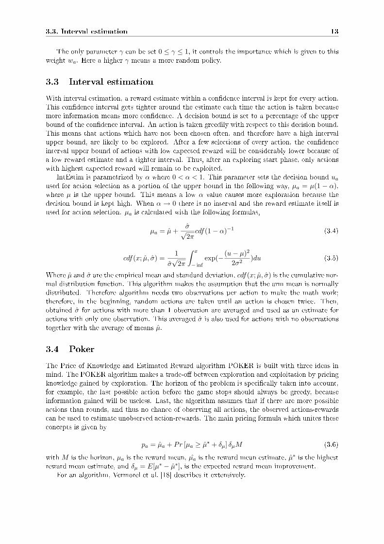
3.3 Interval estimation

With interval estimation, a reward estimate within a con�dence interval is kept for every action.This con�dence interval gets tighter around the estimate each time the action is taken becausemore information means more con�dence. A decision bound is set to a percentage of the upperbound of the con�dence interval. An action is taken greedily with respect to this decision bound.This means that actions which have not been chosen often, and therefore have a high intervalupper bound, are likely to be explored. After a few selections of every action, the con�denceinterval upper bound of actions with low expected reward will be considerably lower because ofa low reward estimate and a tighter interval. Thus, after an exploring start phase, only actionswith highest expected reward will remain to be exploited.

IntEstim is parametrized by α where 0 < α < 1. This parameter sets the decision bound ua

used for action selection as a portion of the upper bound in the following way, µa = µ(1 − α),where µ is the upper bound. This means a low α value causes more exploration because thedecision bound is kept high. When α → 0 there is no interval and the reward estimate itself isused for action selection. µa is calculated with the following formulas,

µa = µ +σ√2π

cdf(1− α)−1 (3.4)

cdf(x; µ, σ) =1

σ√

2π

∫ x

− infexp(−(u− µ)2

2σ2)du (3.5)

Where µ and σ are the empirical mean and standard deviation, cdf(x; µ, σ) is the cumulative nor-mal distribution function. This algorithm makes the assumption that the arm mean is normallydistributed. Therefore algorithm needs two observations per action to make the math work;therefore, in the beginning, random actions are taken until an action is chosen twice. Then,obtained σ for actions with more than 1 observation are averaged and used as an estimate foractions with only one observation. This averaged σ is also used for actions with no observationstogether with the average of means µ.

3.4 Poker

The Price of Knowledge and Estimated Reward algorithm POKER is built with three ideas inmind. The POKER algorithm makes a trade-o� between exploration and exploitation by pricingknowledge gained by exploration. The horizon of the problem is speci�cally taken into account,for example, the last possible action before the game stops should always be greedy, becauseinformation gained will be useless. Last, the algorithm assumes that if there are more possibleactions than rounds, and thus no chance of observing all actions, the observed actions-rewardscan be used to estimate unobserved action-rewards. The main pricing formula which unites theseconcepts is given by

pa = µa + Pr [µa ≥ µ? + δµ] δµM (3.6)

with M is the horizon, µa is the reward mean, µa is the reward mean estimate, µ∗ is the highestreward mean estimate, and δµ = E[µ∗ − µ∗], is the expected reward mean improvement.

For an algorithm, Vermorel et al. [18] describes it extensively.

3.5. UCB2 14

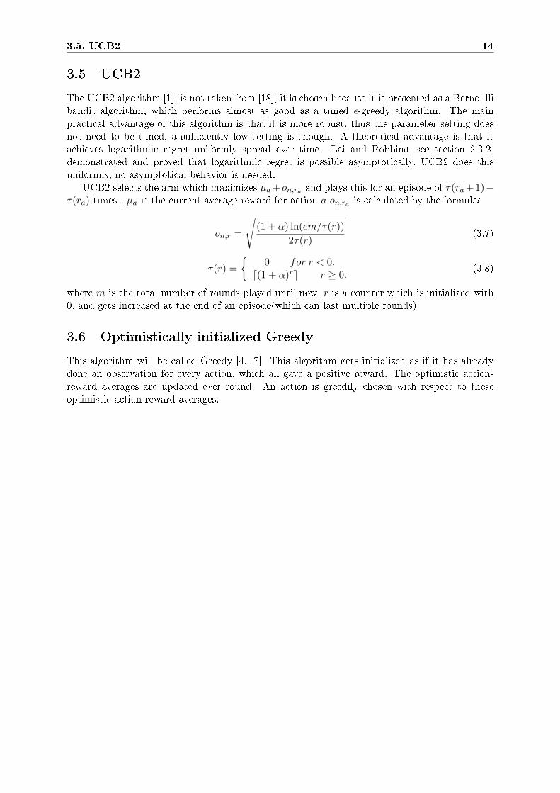
3.5 UCB2

The UCB2 algorithm [1], is not taken from [18], it is chosen because it is presented as a Bernoullibandit algorithm, which performs almost as good as a tuned ε-greedy algorithm. The mainpractical advantage of this algorithm is that it is more robust, thus the parameter setting doesnot need to be tuned, a su�ciently low setting is enough. A theoretical advantage is that itachieves logarithmic regret uniformly spread over time. Lai and Robbins, see section 2.3.2,demonstrated and proved that logarithmic regret is possible asymptotically, UCB2 does thisuniformly, no asymptotical behavior is needed.

UCB2 selects the arm which maximizes µa +on,ra and plays this for an episode of τ(ra +1)−τ(ra) times , µa is the current average reward for action a on,ra is calculated by the formulas

on,r =

√(1 + α) ln(em/τ(r))

2τ(r)(3.7)

τ(r) ={

0 for r < 0.d(1 + α)re r ≥ 0.

(3.8)

where m is the total number of rounds played until now, r is a counter which is initialized with0, and gets increased at the end of an episode(which can last multiple rounds).

3.6 Optimistically initialized Greedy

This algorithm will be called Greedy [4, 17]. This algorithm gets initialized as if it has alreadydone an observation for every action, which all gave a positive reward. The optimistic action-reward averages are updated ever round. An action is greedily chosen with respect to theseoptimistic action-reward averages.

Chapter 4

Experiments

4.1 Overview of experimental setup

This chapter will describe the experiments which where designed to be able to compare the newlyproposed Beetle Bandit algorithm with other algorithms. There will be two setups: a 2-armedbandit setup and a 5-armed setup. These two setups are chosen because the 2-armed banditproblem is the simplest problem which still exhibits the whole complexity of the explorationexploitation trade-o�. The 5-armed bandit is chosen so the results obtained can be compared tothe article of Wang et al. [20]. The obtained results will be discussed at the end of the chapter.One has to take into account that Beetle Bandit is an in�nite horizon algorithm where the otheralgorithms it is being compared to are not. Usually �nite horizon algorithms perform betterthan in�nite horizon algorithms on problems with a small horizon.

4.2 2-Armed bandit experiments

Since we are con�dent the newly reported Beetle Bandit algorithm will make a good trade-o�between exploration and exploitation, we have designed an experiment with a short horizon.This means algorithms with good asymptotic behavior but poor �start" behavior are expected tonot perform well on this setup. This is because they generally over explore in the beginning, thenover exploit in the end, making the poor start behavior. Algorithms are run with parameters setin multiple ways; the best results for every algorithm are reported in this section. UCB2 is theonly algorithm that was run with only 1 parameter because the authors have put this algorithmforward to be robust as long as the parameter α is set low. The authors optimal setting forUCB2 is used.

4.2.1 Experimental setup

The setting uses 2-armed bandit problems. The arms generate Bernoulli distributed rewards,with means drawn uniformly from the interval (0,1) (though all algorithms play the same game)this is done for 20 di�erent games. The game horizon is 20. Every game is played 1000 times.Reward and regret per round will be reported.

Beetle Bandit has a number of parameters, the following parameters are used. To test thein�uence of in�nite vs �nite games played by Beetle Bandit, discount factors γ = 0.99 and 1 wereused. The number of that are sampled is 2000 and the maximal number of basis functions thatwere created was 100. 100 Perseus backups were performed. Every game new basis vectors areinitialized. State sampling of the belief space is performed with the same horizon as the problem.

15

4.3. 5-Armed Beetle experiment 16

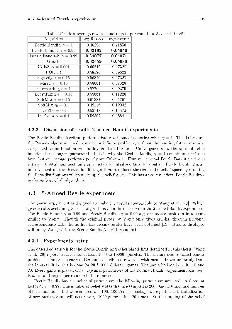
Table 4.1: Best average rewards and regrets per round for 2-armed BanditAlgorithm avg-Reward avg-Regret

Beetle Bandit, γ = 1 0.46298 0.21850

Beetle Bandit, γ = 0.99 0.62192 0.05956

Beetle Bandit-2, γ = 0.99 0.64077 0.04071

Greedy 0.62459 0.05688

UCB2, α = 0.001 0.60819 0.07328

POKER 0.58526 0.09622

ε-greedy, ε = 0.15 0.56346 0.07328

ε-�rst, ε = 0.15 0.58661 0.07328

ε-decreasing, ε = 1 0.58769 0.09379

LeastTaken ε = 0.15 0.58661 0.11220

SoftMax τ = 0.15 0.61387 0.06761

SoftMix τ0 = 0.1 0.49146 0.19002

Exp3 γ = 0.4 0.53718 0.14572

IntEstim α = 0.1 0.59307 0.08841

4.2.2 Discussion of results 2-armed Bandit experiments

The Beetle Bandit algorithm performs badly without discounting when γ = 1. This is becausethe Perseus algorithm used is made for in�nite problems, without discounting future rewards,every next value function will be higher than the last. Convergence onto the optimal valuefunction is no longer guaranteed. This is why the Beetle Bandit, γ = 1 sometimes performsbest, but on average performs poorly see Table 4.1. However, normal Beetle Bandit performswith γ = 0.99 almost best, only optimistically initialized Greedy is better. Beetle Bandit-2 is animprovement on the Beetle Bandit algorithm, it reduces the size of the belief space by orderingthe Beta-distributions which make up the belief space. This has a positive e�ect, Beetle Bandit-2performs best of all algorithms.

4.3 5-Armed Beetle experiment

The 5-arm experiment is designed to make the results comparable to Wang et al. [20]. Whichgives results pertaining to other algorithms than the ones used in the 2-armed Bandit experiment.The Beetle Bandit γ = 0.99 and Beetle Bandit-2 γ = 0.99 algorithms are both run in a setupsimilar to Wang. Though the original paper by Wang only gives graphs, through personalcorrespondence with the author the precise results have been obtained [19]. Results displayedwill be by Wang with the Beetle Bandit Algorithms added.

4.3.1 Experimental setup

The described setup is for the Beetle Bandit and other algorithms described in this thesis, Wanget al. [20] report averages taken from 1000 to 10000 episodes. The setting uses 5-armed banditproblems. The arms generate Bernoulli distributed rewards, with means drawn uniformly fromthe interval (0,1), this is done for 20 * 1000 di�erent games. The game horizon is 5, 10, 15 and20. Every game is played once. Optimal parameters of the 2-armed bandit experiment are used.Reward and regret per round will be reported.

Beetle Bandit has a number of parameters, the following parameters are used. A discountfactor of γ = 0.99. The number of belief states that are sampled is 2000 and the maximal numberof basis functions that were created was 100. 100 Perseus backups were performed. Initializationof new basis vectors will occur every 1000 games, thus 20 times.. State sampling of the belief

4.3. 5-Armed Beetle experiment 17

space is performed with the same horizon as the problem. State sampling of the belief space isdone with the same horizon as the problem.

Table 4.2: Results by Wang et al. compared with Beetle Bandit, 5-armed bandit reward perround is reported

Horizon 5 10 15 20

ε-greedy 0.5905 0.6311 0.6511 0.6703

Bolzman 0.574 0.6244 0.6494 0.6758

Interval Est. 0.498 0.5858 0.6061 0.6313

Thompson 0.5389 0.5965 0.6141 0.6412

MVPI 0.5511 0.6029 0.613 0.6445

Peret Garcia 0.555 0.5887 0.6097 0.6479

Sparse Samp. 0.6075 0.6598 0.6806 0.7148

Bayes Samp 0.6161 0.6686 0.6868 0.7212

Beetle Bandit, γ = 0.99 0.6109 0.6496 0.6673 0.7027

Beetle Bandit-2, γ = 0.99 0.5986 0.6580 0.6697 0,6987

4.3.2 Discussion of results 5-armed Bandit experiments

Table 4.2 shows that Beetle Bandit and Beetle Bandit-2 are comparable in performance on the5-armed bandit. The results for Beetle Bandit are better than those for the classical approaches.However, the Sparse and Bayes sampling techniques are generally a bit better than Beetle Bandit.There are two reason why Beetle Bandits performance does not grow equally with Bayesiansampling. Beetle Bandit is an in�nite horizon algorithm, where Bayesian sampling is a �nitehorizon algorithm. In�nite horizon algorithms usually perform slightly worse than �nite horizonalgorithms which do not discount rewards.

Beetle Bandit also su�ers from the size of the belief space when the horizon of the problemgrows. The reachable belief space can be seen as a tree with the root at the start of a game, thetree branches out with every possible action and reward, this means the size of the tree will be(2K)H , where K is the number of arms and H the horizon. The sampling of the belief spacewhich beetle performs at the beginning of the algorithm is not capable of getting a representativesample of the whole belief space, this the performance of the algorithm drops as the size of thebelief space grows larger.

Chapter 5

Conclusion

In this thesis I have given an overview of Bandit Problems, in particular those with rewardsobtained from Bernoulli distributions. I have given an overview of algorithms with which ournewly developed Beetle Bandit algorithm was compared, as well as the math needed to adjustBeetle into Beetle Bandit. The experiments show that for Bandit problems with limited arms,horizon, and rewards distributed according to a Bernoulli distribution, the Beetle Bandit is per-forming better than classical approaches and slightly worse than other current Bayesian inspiredapproaches. These results occur because Beetle Bandit is an in�nite horizon algorithm whereasthe compared algorithms are �nite horizon algorithms which are usually better at dealing withshort horizon setups such as those presented in this paper. The other cause of these results isthe problem Beetle Bandit has with adequate sampling of large belief spaces. The Bayesian ap-proach taken with Beetle Bandit o�ers the possibility of an optimal exploration vs. exploitationtrade-o�. Beetle Bandit has shown through o�ine pre-computation that the Bayesian approachcan give best results while still being able to make fast online decisions.

The main advantage of Beetle Bandit is its performance on problems with a small number ofvariables. For these problems, it o�ers one of the best exploration exploitation decision makingavailable. However, a problem still facing Beetle and Beetle Bandit are larger problems withmore variables. This is partly due to the size of the belief space, as sampling this e�cientlybecomes increasingly harder and the projection onto a �xed set of basis functions becomes moreprone to errors as the size of the belief space increases. I have made a start at improving thisvulnerability of Beetle Bandit by sorting the distributions making up the belief space. Theresults of this approach are promising, as for small problems the 'adapted' Beetle Bandit-2 doesnot perform worse, but sometimes even better than Beetle Bandit. Making Beetle Bandit scaleto larger problems is the main area of future research. One may think of more intelligent beliefspace sampling, better belief space representations, or better projection onto basis functions. Another way can be to keep the look ahead decision tree small by intelligent sampling techniques.A �rst step into this future research has been given with Beetle Bandit-2. For in terms ofpractical applications, one can think of intelligent adaptive routers which can use Beetle Banditin discovering what peers should be selected for optimal service. Beetle Bandit can also beused in adaptive medical trials where the goal is to decide which is the better treatment while,balancing this with the the least possible negative impact.

18

Bibliography

[1] P. Auer, N. Cesa-Bianchi, and P. Fischer. Finite-time analysis of the multiarmed banditproblem. Machine Learning, 47(2/3):235�256, 2002.

[2] P. Auer, N. Cesa-Bianchi, Y. Freund, and R. E. Schapire. Gambling in a rigged casino:the adversarial multi-armed bandit problem. In Proceedings of the 36th Annual Symposium

on Foundations of Computer Science, pages 322�331. IEEE Computer Society Press, LosAlamitos, CA, 1995.

[3] R. Bellman. A problem in the sequential design of experiments. Sankhya A, 16:221�229,1956.

[4] R. I. Brafman and M. Tennenholtz. R-MAX � a general polynomial time algorithm fornear-optimal reinforcement learning. In IJCAI, pages 953�958, 2001.

[5] V. Cicirello and S. Smith. The max k-armed bandit: A new model for exploration applied tosearch heuristic selection. In 20th National Conference on Arti�cial Intelligence (AAAI-05),July 2005. Best Paper Award.

[6] T. M. Cover and J. A. Thomas. Elements of Information Theory. John Wiley, New York,1991.

[7] M. O. Du�. Q-learning for bandit problems. In International Conference on Machine

Learning, pages 209�217, 1995.

[8] M. O. Du�. Optimal learning: computational procedures for Bayes-adaptive Markov decision

processes. PhD thesis, University of Massachusetts Amherst, 2002. Director-Andrew Barto.

[9] J. Gittins. Bandit Processes and Dynamic Allocation Indices. John Wiley, 1989.

[10] J. C. Gittins and D. M. Jones. A dynamic allocation index for the sequential design ofexperiments. Progress in Statistics, 1:241�66, 1974.

[11] J. Hardwick. IMS Lecture Notes � Monograph Series, chapter A modi�ed bandit as anapproach to ethical allocation in clinical trials, pages 65�87. Institute of MathematicalStatistics, 1995.

[12] J. Hardwick, R. Oehmke, and Q. F. Stout. New adaptive designs for delayed responsemodels. Journal of Sequential Planning and Inference, 136:1940�1955, 2006.

[13] T. Lai and H. Robbins. Asymptotically e�cient adaptive allocation rules. Advances in

Mathematics, 6:4�22, 1985.

[14] P. Poupart, N. Vlassis, J. Hoey, and K. Regan. An analytic solution to discrete Bayesianreinforcement learning. In Proceedings of the International Joint Conference on Machine

Learning, pages 249�256, Hakodate, Japan, May 2006.

19

Bibliography 20

[15] H. Robbins. Some aspects of the sequential design of experiments. Bulletin American

Mathematical Society, 55:427�535, 1952.

[16] M. T. J. Spaan and N. Vlassis. Perseus: Randomized point-based value iteration forPOMDPs. Journal of Arti�cial Intelligence Research, 24:195�220, 2005.

[17] R. S. Sutton and A. G. Barto. Reinforcement Learning. MIT Press, Cambridge, MA, 1998.

[18] J. Vermorel and M. Mohri. Multi-armed bandit algorithms and empirical evaluation. InMachine Learning: ECML 2005: 16th European Conference on Machine Learning, Porto,

Portugal, October 3-7, 2005. Proceedings, volume Volume 3720, pages 437 � 448, Nov 2005.

[19] T. Wang. Personal correspondence, June 2006.

[20] T. Wang, D. Lizotte, M. Bowling, and D. Schuurmans. Bayesian sparse sampling for on-linereward optimization. In ICML '05: Proceedings of the 22nd international conference on

Machine learning, pages 956�963, New York, NY, USA, 2005. ACM Press.