Embed Size (px)
Citation preview

IntroductionUnconstrained Optimization
Review: Simultaneous systems of equationsThe Tangent Plane
BEE1024 Mathematics for EconomistsMultivariate Functions
Juliette Stephenson and Amr (Miro) AlgarhiAuthor: Dieter Balkenborg
Department of Economics, University of Exeter
Week 2
Balkenborg Multivariate Functions
IntroductionUnconstrained Optimization
Review: Simultaneous systems of equationsThe Tangent Plane
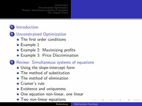
1 Introduction
2 Unconstrained OptimizationThe �rst order conditionsExample 1Example 2: Maximizing pro�tsExample 3: Price Discrimination
3 Review: Simultaneous systems of equationsUsing the slope-intercept formThe method of substitutionThe method of eliminationCramer�s ruleExistence and uniquenessOne equation non-linear, one linearTwo non-linear equations
Balkenborg Multivariate Functions
IntroductionUnconstrained Optimization
Review: Simultaneous systems of equationsThe Tangent Plane
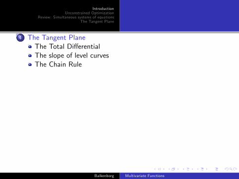
4 The Tangent PlaneThe Total Di¤erentialThe slope of level curvesThe Chain Rule
Balkenborg Multivariate Functions

IntroductionUnconstrained Optimization
Review: Simultaneous systems of equationsThe Tangent Plane
Optimization 1
�Since the fabric of the universe is most perfect, andis the work of a most perfect creator, nothing whatsoevertakes place in the universe in which some form ofmaximum or minimum does not appear.�Leonhard Euler, 1744
Balkenborg Multivariate Functions
IntroductionUnconstrained Optimization
Review: Simultaneous systems of equationsThe Tangent Plane
Objectives
Subject: Optimization of multivariate functions
Two basic types of problems:
1 unconstrained (e.g. pro�t maximization)2 constrained (e.g. utility maximization with budget constraint)
This week:
1 ��rst order conditions� for optimum2 Simultaneous system of equations (!Review)3 the tangent plane / the marginal rate of substitution
Next weeks:
1 Lagrangian approach for constrained problems2 2nd order conditions
Balkenborg Multivariate Functions
IntroductionUnconstrained Optimization
Review: Simultaneous systems of equationsThe Tangent Plane
Objectives
Subject: Optimization of multivariate functions
Two basic types of problems:1 unconstrained (e.g. pro�t maximization)
2 constrained (e.g. utility maximization with budget constraint)
This week:
1 ��rst order conditions� for optimum2 Simultaneous system of equations (!Review)3 the tangent plane / the marginal rate of substitution
Next weeks:
1 Lagrangian approach for constrained problems2 2nd order conditions
Balkenborg Multivariate Functions
IntroductionUnconstrained Optimization
Review: Simultaneous systems of equationsThe Tangent Plane
Objectives
Subject: Optimization of multivariate functions
Two basic types of problems:1 unconstrained (e.g. pro�t maximization)2 constrained (e.g. utility maximization with budget constraint)
This week:
1 ��rst order conditions� for optimum2 Simultaneous system of equations (!Review)3 the tangent plane / the marginal rate of substitution
Next weeks:
1 Lagrangian approach for constrained problems2 2nd order conditions
Balkenborg Multivariate Functions
IntroductionUnconstrained Optimization
Review: Simultaneous systems of equationsThe Tangent Plane
Objectives
Subject: Optimization of multivariate functions
Two basic types of problems:1 unconstrained (e.g. pro�t maximization)2 constrained (e.g. utility maximization with budget constraint)
This week:1 ��rst order conditions� for optimum
2 Simultaneous system of equations (!Review)3 the tangent plane / the marginal rate of substitution
Next weeks:
1 Lagrangian approach for constrained problems2 2nd order conditions
Balkenborg Multivariate Functions
IntroductionUnconstrained Optimization
Review: Simultaneous systems of equationsThe Tangent Plane
Objectives
Subject: Optimization of multivariate functions
Two basic types of problems:1 unconstrained (e.g. pro�t maximization)2 constrained (e.g. utility maximization with budget constraint)
This week:1 ��rst order conditions� for optimum2 Simultaneous system of equations (!Review)
3 the tangent plane / the marginal rate of substitution
Next weeks:
1 Lagrangian approach for constrained problems2 2nd order conditions
Balkenborg Multivariate Functions
IntroductionUnconstrained Optimization
Review: Simultaneous systems of equationsThe Tangent Plane
Objectives
Subject: Optimization of multivariate functions
Two basic types of problems:1 unconstrained (e.g. pro�t maximization)2 constrained (e.g. utility maximization with budget constraint)
This week:1 ��rst order conditions� for optimum2 Simultaneous system of equations (!Review)3 the tangent plane / the marginal rate of substitution
Next weeks:1 Lagrangian approach for constrained problems
2 2nd order conditions
Balkenborg Multivariate Functions
IntroductionUnconstrained Optimization
Review: Simultaneous systems of equationsThe Tangent Plane
Objectives
Subject: Optimization of multivariate functions
Two basic types of problems:1 unconstrained (e.g. pro�t maximization)2 constrained (e.g. utility maximization with budget constraint)
This week:1 ��rst order conditions� for optimum2 Simultaneous system of equations (!Review)3 the tangent plane / the marginal rate of substitution
Next weeks:1 Lagrangian approach for constrained problems2 2nd order conditions
Balkenborg Multivariate Functions
IntroductionUnconstrained Optimization
Review: Simultaneous systems of equationsThe Tangent Plane
The �rst order conditionsExample 1Example 2: Maximizing pro�tsExample 3: Price Discrimination
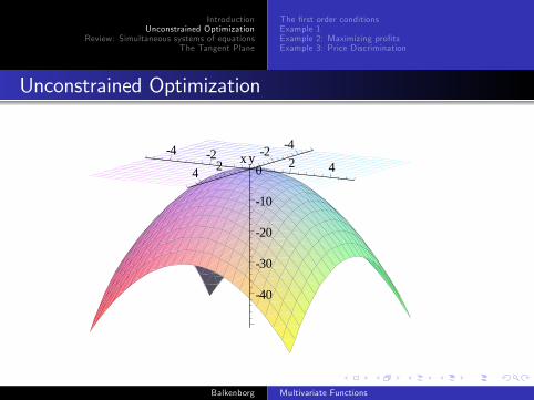
Unconstrained Optimization
40
30
20
10
04 2 2 4
y42
24x
Balkenborg Multivariate Functions
IntroductionUnconstrained Optimization
Review: Simultaneous systems of equationsThe Tangent Plane
The �rst order conditionsExample 1Example 2: Maximizing pro�tsExample 3: Price Discrimination
Unconstrained Optimization
Objective: Find (absolute) maximum of function
z = f (x , y)
i.e., �nd a pair (x�, y �) such that
f (x�, y �) � f (x , y)
holds for all pairs (x , y).Hereby both pairs of numbers (x�, y �) and (x , y) must be in the domain ofthe function.
For an absolute minimum require f (x�, y �) � f (x , y).f (x , y) is called the �objective function�.
Balkenborg Multivariate Functions
IntroductionUnconstrained Optimization
Review: Simultaneous systems of equationsThe Tangent Plane
The �rst order conditionsExample 1Example 2: Maximizing pro�tsExample 3: Price Discrimination
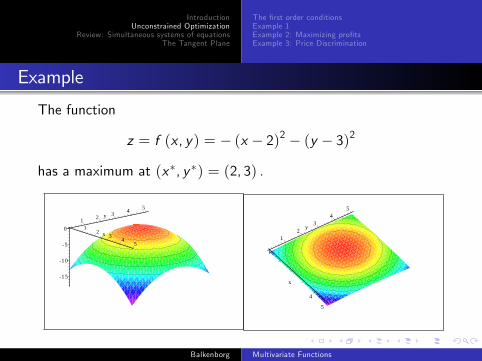
Example
The function
z = f (x , y) = � (x � 2)2 � (y � 3)2
has a maximum at (x�, y �) = (2, 3) .
15
10
5
01 2 3 4 5
y
12
34
5
x1
23
45
y
4
5
x
Balkenborg Multivariate Functions
IntroductionUnconstrained Optimization
Review: Simultaneous systems of equationsThe Tangent Plane
The �rst order conditionsExample 1Example 2: Maximizing pro�tsExample 3: Price Discrimination
Outline1 Introduction2 Unconstrained Optimization
The �rst order conditionsExample 1Example 2: Maximizing pro�tsExample 3: Price Discrimination
3 Review: Simultaneous systems of equationsUsing the slope-intercept formThe method of substitutionThe method of eliminationCramer�s ruleExistence and uniquenessOne equation non-linear, one linearTwo non-linear equations
4 The Tangent PlaneThe Total Di¤erentialThe slope of level curvesThe Chain Rule Balkenborg Multivariate Functions
IntroductionUnconstrained Optimization
Review: Simultaneous systems of equationsThe Tangent Plane
The �rst order conditionsExample 1Example 2: Maximizing pro�tsExample 3: Price Discrimination
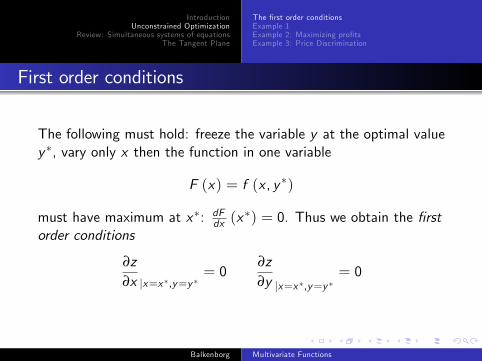
First order conditions
The following must hold: freeze the variable y at the optimal valuey �, vary only x then the function in one variable
F (x) = f (x , y �)
must have maximum at x�: dFdx (x�) = 0. Thus we obtain the �rst
order conditions
∂z∂x jx=x �,y=y �
= 0∂z∂y jx=x �,y=y �
= 0
Balkenborg Multivariate Functions
IntroductionUnconstrained Optimization
Review: Simultaneous systems of equationsThe Tangent Plane
The �rst order conditionsExample 1Example 2: Maximizing pro�tsExample 3: Price Discrimination
Outline1 Introduction2 Unconstrained Optimization
The �rst order conditionsExample 1Example 2: Maximizing pro�tsExample 3: Price Discrimination
3 Review: Simultaneous systems of equationsUsing the slope-intercept formThe method of substitutionThe method of eliminationCramer�s ruleExistence and uniquenessOne equation non-linear, one linearTwo non-linear equations
4 The Tangent PlaneThe Total Di¤erentialThe slope of level curvesThe Chain Rule Balkenborg Multivariate Functions
IntroductionUnconstrained Optimization
Review: Simultaneous systems of equationsThe Tangent Plane
The �rst order conditionsExample 1Example 2: Maximizing pro�tsExample 3: Price Discrimination
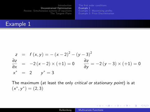
Example 1
z = f (x , y) = � (x � 2)2 � (y � 3)2
∂z∂x
= �2 (x � 2)� (+1) = 0 ∂z∂y= �2 (y � 3)� (+1) = 0
x� = 2 y � = 3
The maximum (at least the only critical or stationary point) is at(x�, y �) = (2, 3)
Balkenborg Multivariate Functions
IntroductionUnconstrained Optimization
Review: Simultaneous systems of equationsThe Tangent Plane
The �rst order conditionsExample 1Example 2: Maximizing pro�tsExample 3: Price Discrimination
Outline1 Introduction2 Unconstrained Optimization
The �rst order conditionsExample 1Example 2: Maximizing pro�tsExample 3: Price Discrimination
3 Review: Simultaneous systems of equationsUsing the slope-intercept formThe method of substitutionThe method of eliminationCramer�s ruleExistence and uniquenessOne equation non-linear, one linearTwo non-linear equations
4 The Tangent PlaneThe Total Di¤erentialThe slope of level curvesThe Chain Rule Balkenborg Multivariate Functions
IntroductionUnconstrained Optimization
Review: Simultaneous systems of equationsThe Tangent Plane
The �rst order conditionsExample 1Example 2: Maximizing pro�tsExample 3: Price Discrimination
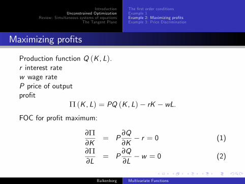
Maximizing pro�ts
Production function Q (K , L).r interest ratew wage rateP price of outputpro�t
Π (K , L) = PQ (K , L)� rK � wL.FOC for pro�t maximum:
∂Π∂K
= P∂Q∂K
� r = 0 (1)
∂Π∂L
= P∂Q∂L� w = 0 (2)
Balkenborg Multivariate Functions
IntroductionUnconstrained Optimization
Review: Simultaneous systems of equationsThe Tangent Plane
The �rst order conditionsExample 1Example 2: Maximizing pro�tsExample 3: Price Discrimination
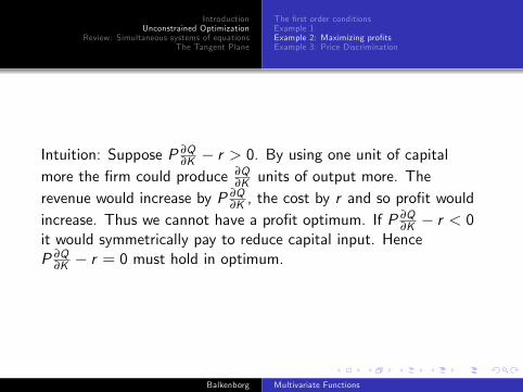
Intuition: Suppose P ∂Q∂K � r > 0. By using one unit of capital
more the �rm could produce ∂Q∂K units of output more. The
revenue would increase by P ∂Q∂K , the cost by r and so pro�t would
increase. Thus we cannot have a pro�t optimum. If P ∂Q∂K � r < 0
it would symmetrically pay to reduce capital input. HenceP ∂Q
∂K � r = 0 must hold in optimum.
Balkenborg Multivariate Functions
IntroductionUnconstrained Optimization
Review: Simultaneous systems of equationsThe Tangent Plane
The �rst order conditionsExample 1Example 2: Maximizing pro�tsExample 3: Price Discrimination
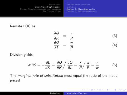
Rewrite FOC as
∂Q∂K
=rP
(3)
∂Q∂L
=wP
(4)
Division yields:
MRS = � dLdK
=∂Q∂K
�∂Q∂L
=rP
. wP=rw
(5)
The marginal rate of substitution must equal the ratio of the inputprices!
Balkenborg Multivariate Functions
IntroductionUnconstrained Optimization
Review: Simultaneous systems of equationsThe Tangent Plane
The �rst order conditionsExample 1Example 2: Maximizing pro�tsExample 3: Price Discrimination
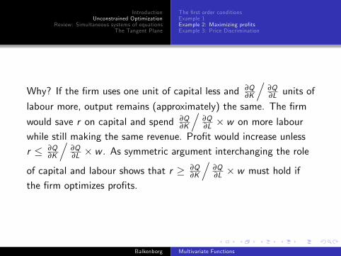
Why? If the �rm uses one unit of capital less and ∂Q∂K
.∂Q∂L units of
labour more, output remains (approximately) the same. The �rm
would save r on capital and spend ∂Q∂K
.∂Q∂L � w on more labour
while still making the same revenue. Pro�t would increase unlessr � ∂Q
∂K
.∂Q∂L � w . As symmetric argument interchanging the role
of capital and labour shows that r � ∂Q∂K
.∂Q∂L � w must hold if
the �rm optimizes pro�ts.
Balkenborg Multivariate Functions
IntroductionUnconstrained Optimization
Review: Simultaneous systems of equationsThe Tangent Plane
The �rst order conditionsExample 1Example 2: Maximizing pro�tsExample 3: Price Discrimination
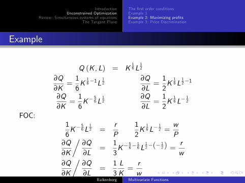
Example
Q (K , L) = K16 L
12
∂Q∂K
=16K
16�1L
12
∂Q∂L
=12K
16 L
12�1
∂Q∂K
=16K�
56 L
12
∂Q∂L
=12K
16 L�
12
FOC:16K�
56 L
12 =
rP
12K
16 L�
12 =
wP
∂Q∂K
�∂Q∂L
=13K�
56�
16 L
12�(�
12 ) =
rw
∂Q∂K
�∂Q∂L
=13LK=rw
Balkenborg Multivariate Functions
IntroductionUnconstrained Optimization
Review: Simultaneous systems of equationsThe Tangent Plane
The �rst order conditionsExample 1Example 2: Maximizing pro�tsExample 3: Price Discrimination
Example
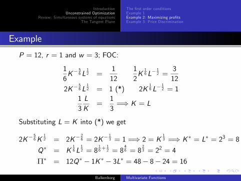
P = 12, r = 1 and w = 3; FOC:
16K�
56 L
12 =
112
12K
16 L�
12 =
312
2K�56 L
12 = 1 (*) 2K
16 L�
12 = 1
13LK
=13=) K = L
Substituting L = K into (*) we get
2K�56K
12 = 2K�
26 = 2K�
13 = 1 =) 2 = K
13 =) K � = L� = 23 = 8
Q� = K16 L
12 = 8
16+
12 = 8
46 = 8
23 = 22 = 4
Π� = 12Q� � 1K � � 3L� = 48� 8� 24 = 16
Balkenborg Multivariate Functions
IntroductionUnconstrained Optimization
Review: Simultaneous systems of equationsThe Tangent Plane
The �rst order conditionsExample 1Example 2: Maximizing pro�tsExample 3: Price Discrimination
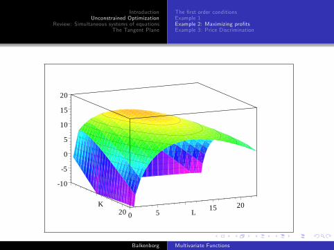
20K
0 515 20
L
10
5
0
5
10
15
20
Balkenborg Multivariate Functions
IntroductionUnconstrained Optimization
Review: Simultaneous systems of equationsThe Tangent Plane
The �rst order conditionsExample 1Example 2: Maximizing pro�tsExample 3: Price Discrimination
Outline1 Introduction2 Unconstrained Optimization
The �rst order conditionsExample 1Example 2: Maximizing pro�tsExample 3: Price Discrimination
3 Review: Simultaneous systems of equationsUsing the slope-intercept formThe method of substitutionThe method of eliminationCramer�s ruleExistence and uniquenessOne equation non-linear, one linearTwo non-linear equations
4 The Tangent PlaneThe Total Di¤erentialThe slope of level curvesThe Chain Rule Balkenborg Multivariate Functions
IntroductionUnconstrained Optimization
Review: Simultaneous systems of equationsThe Tangent Plane
The �rst order conditionsExample 1Example 2: Maximizing pro�tsExample 3: Price Discrimination
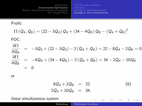
Example 3: Price Discrimination
A monopolist with total cost function TC (Q) = Q2 sells hisproduct in two di¤erent countries. When he sells QA units of thegood in country A he will obtain the price
PA = 22� 3QA
for each unit. When he sells QB units of the good in country B heobtains the price
PB = 34� 4QB .How much should the monopolist sell in the two countries in orderto maximize pro�ts?
Balkenborg Multivariate Functions
IntroductionUnconstrained Optimization
Review: Simultaneous systems of equationsThe Tangent Plane
The �rst order conditionsExample 1Example 2: Maximizing pro�tsExample 3: Price Discrimination
Solution
Total revenue in country A:
TRA = PAQA = (22� 3QA)QA
Total revenue in country B:
TRB = PBQB = (34� 4QB )QB
Total production costs are:
TC = (QA +QB )2
Pro�t:
Π (QA,QB ) = (22� 3QA)QA + (34� 4QB )QB � (QA +QB )2
Balkenborg Multivariate Functions
IntroductionUnconstrained Optimization
Review: Simultaneous systems of equationsThe Tangent Plane
The �rst order conditionsExample 1Example 2: Maximizing pro�tsExample 3: Price Discrimination
Pro�t:
Π (QA,QB ) = (22� 3QA)QA + (34� 4QB )QB � (QA +QB )2
FOC:
∂Π∂QA
= �3QA + (22� 3QA)� 2 (QA +QB ) = 22� 8QA � 2QB = 0
∂Π∂QB
= �4QB + (34� 4QB )� 2 (QA +QB ) = 34� 2QA � 10QB= 0
or
8QA + 2QB = 22 (6)
2QA + 10QB = 34.
linear simultaneous systemBalkenborg Multivariate Functions
IntroductionUnconstrained Optimization
Review: Simultaneous systems of equationsThe Tangent Plane
Using the slope-intercept formThe method of substitutionThe method of eliminationCramer�s ruleExistence and uniquenessOne equation non-linear, one linearTwo non-linear equations
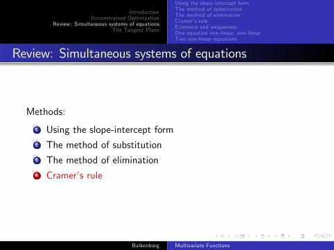
Review: Simultaneous systems of equations
Methods:
1 Using the slope-intercept form
2 The method of substitution3 The method of elimination4 Cramer�s rule
Balkenborg Multivariate Functions
IntroductionUnconstrained Optimization
Review: Simultaneous systems of equationsThe Tangent Plane
Using the slope-intercept formThe method of substitutionThe method of eliminationCramer�s ruleExistence and uniquenessOne equation non-linear, one linearTwo non-linear equations
Review: Simultaneous systems of equations
Methods:
1 Using the slope-intercept form2 The method of substitution
3 The method of elimination4 Cramer�s rule
Balkenborg Multivariate Functions
IntroductionUnconstrained Optimization
Review: Simultaneous systems of equationsThe Tangent Plane
Using the slope-intercept formThe method of substitutionThe method of eliminationCramer�s ruleExistence and uniquenessOne equation non-linear, one linearTwo non-linear equations
Review: Simultaneous systems of equations
Methods:
1 Using the slope-intercept form2 The method of substitution3 The method of elimination
4 Cramer�s rule
Balkenborg Multivariate Functions
IntroductionUnconstrained Optimization
Review: Simultaneous systems of equationsThe Tangent Plane
Using the slope-intercept formThe method of substitutionThe method of eliminationCramer�s ruleExistence and uniquenessOne equation non-linear, one linearTwo non-linear equations
Review: Simultaneous systems of equations
Methods:
1 Using the slope-intercept form2 The method of substitution3 The method of elimination4 Cramer�s rule
Balkenborg Multivariate Functions
IntroductionUnconstrained Optimization
Review: Simultaneous systems of equationsThe Tangent Plane
Using the slope-intercept formThe method of substitutionThe method of eliminationCramer�s ruleExistence and uniquenessOne equation non-linear, one linearTwo non-linear equations
Outline1 Introduction2 Unconstrained Optimization
The �rst order conditionsExample 1Example 2: Maximizing pro�tsExample 3: Price Discrimination
3 Review: Simultaneous systems of equationsUsing the slope-intercept formThe method of substitutionThe method of eliminationCramer�s ruleExistence and uniquenessOne equation non-linear, one linearTwo non-linear equations
4 The Tangent PlaneThe Total Di¤erentialThe slope of level curvesThe Chain Rule Balkenborg Multivariate Functions
IntroductionUnconstrained Optimization
Review: Simultaneous systems of equationsThe Tangent Plane
Using the slope-intercept formThe method of substitutionThe method of eliminationCramer�s ruleExistence and uniquenessOne equation non-linear, one linearTwo non-linear equations
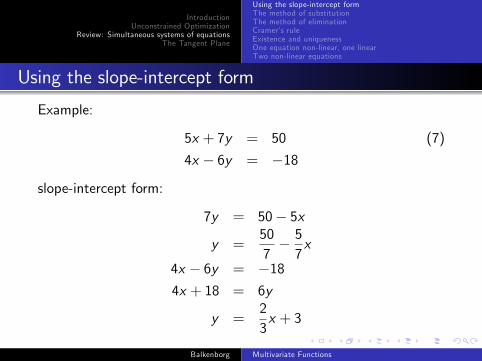
Using the slope-intercept form
Example:
5x + 7y = 50 (7)
4x � 6y = �18
slope-intercept form:
7y = 50� 5x
y =507� 57x
4x � 6y = �184x + 18 = 6y
y =23x + 3
Balkenborg Multivariate Functions
IntroductionUnconstrained Optimization
Review: Simultaneous systems of equationsThe Tangent Plane
Using the slope-intercept formThe method of substitutionThe method of eliminationCramer�s ruleExistence and uniquenessOne equation non-linear, one linearTwo non-linear equations
2
3
4
5
6
7
8
2 0 2 4 6x
Balkenborg Multivariate Functions
IntroductionUnconstrained Optimization
Review: Simultaneous systems of equationsThe Tangent Plane
Using the slope-intercept formThe method of substitutionThe method of eliminationCramer�s ruleExistence and uniquenessOne equation non-linear, one linearTwo non-linear equations
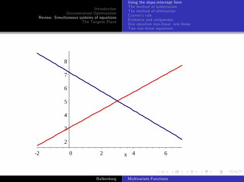
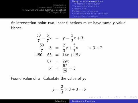
At intersection point two linear functions must have same y -value.Hence
507� 57x = y =
23x + 3
507� 3 =
23x +
57x j � 3� 7
150� 63 = 14x + 15x
87 = 29x
x =8729= 3
Found value of x . Calculate the value of y :
y =23� 3+ 3 = 5
Balkenborg Multivariate Functions
IntroductionUnconstrained Optimization
Review: Simultaneous systems of equationsThe Tangent Plane
Using the slope-intercept formThe method of substitutionThe method of eliminationCramer�s ruleExistence and uniquenessOne equation non-linear, one linearTwo non-linear equations
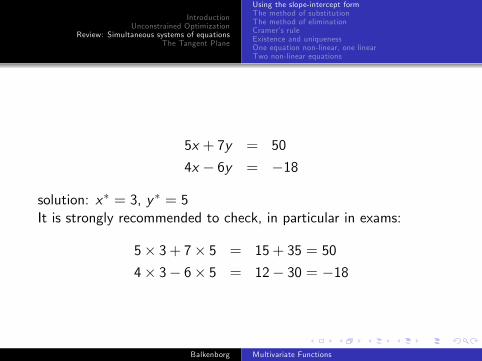
5x + 7y = 50
4x � 6y = �18
solution: x� = 3, y � = 5It is strongly recommended to check, in particular in exams:
5� 3+ 7� 5 = 15+ 35 = 50
4� 3� 6� 5 = 12� 30 = �18
Balkenborg Multivariate Functions
IntroductionUnconstrained Optimization
Review: Simultaneous systems of equationsThe Tangent Plane
Using the slope-intercept formThe method of substitutionThe method of eliminationCramer�s ruleExistence and uniquenessOne equation non-linear, one linearTwo non-linear equations
Outline1 Introduction2 Unconstrained Optimization
The �rst order conditionsExample 1Example 2: Maximizing pro�tsExample 3: Price Discrimination
3 Review: Simultaneous systems of equationsUsing the slope-intercept formThe method of substitutionThe method of eliminationCramer�s ruleExistence and uniquenessOne equation non-linear, one linearTwo non-linear equations
4 The Tangent PlaneThe Total Di¤erentialThe slope of level curvesThe Chain Rule Balkenborg Multivariate Functions
IntroductionUnconstrained Optimization
Review: Simultaneous systems of equationsThe Tangent Plane
Using the slope-intercept formThe method of substitutionThe method of eliminationCramer�s ruleExistence and uniquenessOne equation non-linear, one linearTwo non-linear equations
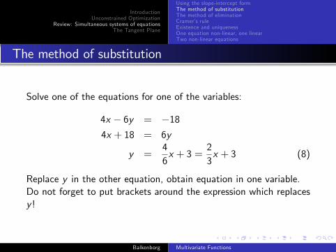
The method of substitution
Solve one of the equations for one of the variables:
4x � 6y = �184x + 18 = 6y
y =46x + 3 =
23x + 3 (8)
Replace y in the other equation, obtain equation in one variable.Do not forget to put brackets around the expression which replacesy !
Balkenborg Multivariate Functions
IntroductionUnconstrained Optimization
Review: Simultaneous systems of equationsThe Tangent Plane
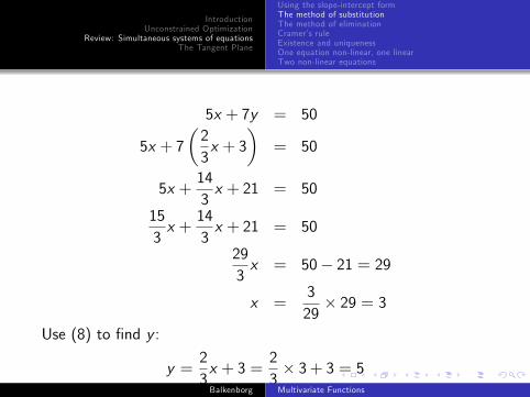
Using the slope-intercept formThe method of substitutionThe method of eliminationCramer�s ruleExistence and uniquenessOne equation non-linear, one linearTwo non-linear equations
5x + 7y = 50
5x + 7�23x + 3
�= 50
5x +143x + 21 = 50
153x +
143x + 21 = 50
293x = 50� 21 = 29
x =329� 29 = 3
Use (8) to �nd y :
y =23x + 3 =
23� 3+ 3 = 5
Balkenborg Multivariate Functions
IntroductionUnconstrained Optimization
Review: Simultaneous systems of equationsThe Tangent Plane
Using the slope-intercept formThe method of substitutionThe method of eliminationCramer�s ruleExistence and uniquenessOne equation non-linear, one linearTwo non-linear equations
Outline1 Introduction2 Unconstrained Optimization
The �rst order conditionsExample 1Example 2: Maximizing pro�tsExample 3: Price Discrimination
3 Review: Simultaneous systems of equationsUsing the slope-intercept formThe method of substitutionThe method of eliminationCramer�s ruleExistence and uniquenessOne equation non-linear, one linearTwo non-linear equations
4 The Tangent PlaneThe Total Di¤erentialThe slope of level curvesThe Chain Rule Balkenborg Multivariate Functions
IntroductionUnconstrained Optimization
Review: Simultaneous systems of equationsThe Tangent Plane
Using the slope-intercept formThe method of substitutionThe method of eliminationCramer�s ruleExistence and uniquenessOne equation non-linear, one linearTwo non-linear equations
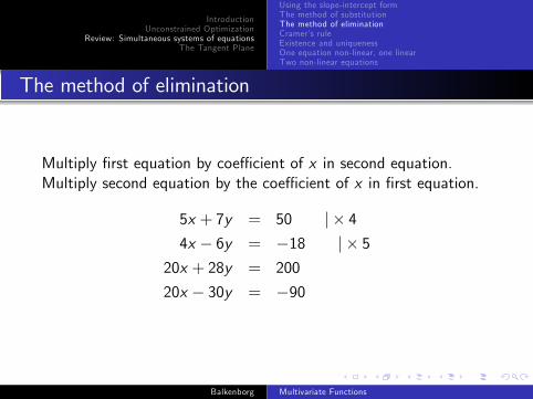
The method of elimination
Multiply �rst equation by coe¢ cient of x in second equation.Multiply second equation by the coe¢ cient of x in �rst equation.
5x + 7y = 50 j � 44x � 6y = �18 j � 5
20x + 28y = 200
20x � 30y = �90
Balkenborg Multivariate Functions
IntroductionUnconstrained Optimization
Review: Simultaneous systems of equationsThe Tangent Plane
Using the slope-intercept formThe method of substitutionThe method of eliminationCramer�s ruleExistence and uniquenessOne equation non-linear, one linearTwo non-linear equations
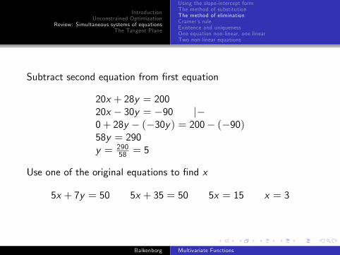
Subtract second equation from �rst equation
20x + 28y = 20020x � 30y = �90 j�0+ 28y � (�30y) = 200� (�90)58y = 290y = 290
58 = 5
Use one of the original equations to �nd x
5x + 7y = 50 5x + 35 = 50 5x = 15 x = 3
Balkenborg Multivariate Functions
IntroductionUnconstrained Optimization
Review: Simultaneous systems of equationsThe Tangent Plane
Using the slope-intercept formThe method of substitutionThe method of eliminationCramer�s ruleExistence and uniquenessOne equation non-linear, one linearTwo non-linear equations
Outline1 Introduction2 Unconstrained Optimization
The �rst order conditionsExample 1Example 2: Maximizing pro�tsExample 3: Price Discrimination
3 Review: Simultaneous systems of equationsUsing the slope-intercept formThe method of substitutionThe method of eliminationCramer�s ruleExistence and uniquenessOne equation non-linear, one linearTwo non-linear equations
4 The Tangent PlaneThe Total Di¤erentialThe slope of level curvesThe Chain Rule Balkenborg Multivariate Functions
IntroductionUnconstrained Optimization
Review: Simultaneous systems of equationsThe Tangent Plane
Using the slope-intercept formThe method of substitutionThe method of eliminationCramer�s ruleExistence and uniquenessOne equation non-linear, one linearTwo non-linear equations
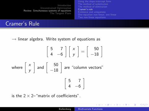
Cramer�s Rule
! linear algebra. Write system of equations as�5 74 �6
� �xy
�=
�50
�18
�
where�xy
�and
�50
�18
�are �column vectors�
�5 74 �6
�is the 2� 2��matrix of coe¢ cients�.
Balkenborg Multivariate Functions
IntroductionUnconstrained Optimization
Review: Simultaneous systems of equationsThe Tangent Plane
Using the slope-intercept formThe method of substitutionThe method of eliminationCramer�s ruleExistence and uniquenessOne equation non-linear, one linearTwo non-linear equations
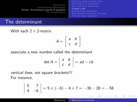
The determinant
With each 2� 2-matrix
A =�a bc d
�associate a new number called the determinant
detA =
���� a bc d
���� = ad � cbvertical lines, not square brackets!!!For instance,���� 5 7
4 �6
���� = 5� (�6)� 4� 7 = �30� 28 = �58Balkenborg Multivariate Functions
IntroductionUnconstrained Optimization
Review: Simultaneous systems of equationsThe Tangent Plane
Using the slope-intercept formThe method of substitutionThe method of eliminationCramer�s ruleExistence and uniquenessOne equation non-linear, one linearTwo non-linear equations
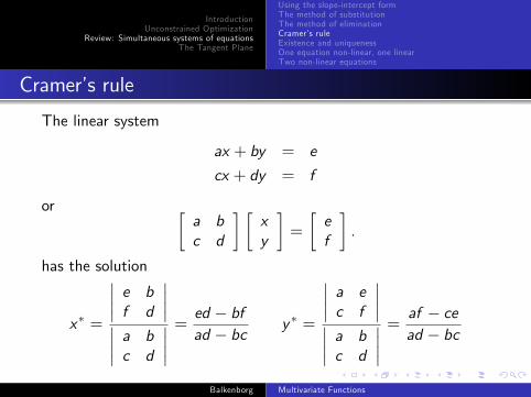
Cramer�s rule
The linear system
ax + by = e
cx + dy = f
or �a bc d
� �xy
�=
�ef
�.
has the solution
x� =
���� e bf d
�������� a bc d
���� =ed � bfad � bc y � =
���� a ec f
�������� a bc d
���� =af � cead � bc
Balkenborg Multivariate Functions
IntroductionUnconstrained Optimization
Review: Simultaneous systems of equationsThe Tangent Plane
Using the slope-intercept formThe method of substitutionThe method of eliminationCramer�s ruleExistence and uniquenessOne equation non-linear, one linearTwo non-linear equations
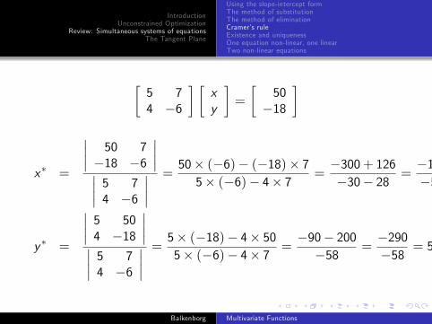
�5 74 �6
� �xy
�=
�50
�18
�
x� =
���� 50 7�18 �6
�������� 5 74 �6
���� =50� (�6)� (�18)� 75� (�6)� 4� 7 =
�300+ 126�30� 28 =
�174�58 = 3
y � =
���� 5 504 �18
�������� 5 74 �6
���� =5� (�18)� 4� 505� (�6)� 4� 7 =
�90� 200�58 =
�290�58 = 5
Balkenborg Multivariate Functions
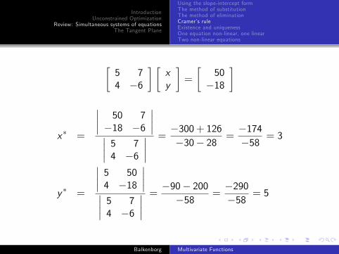
IntroductionUnconstrained Optimization
Review: Simultaneous systems of equationsThe Tangent Plane
Using the slope-intercept formThe method of substitutionThe method of eliminationCramer�s ruleExistence and uniquenessOne equation non-linear, one linearTwo non-linear equations
�5 74 �6
� �xy
�=
�50
�18
�
x� =
���� 50 7�18 �6
�������� 5 74 �6
���� =�300+ 126�30� 28 =
�174�58 = 3
y � =
���� 5 504 �18
�������� 5 74 �6
���� =�90� 200�58 =
�290�58 = 5
Balkenborg Multivariate Functions
IntroductionUnconstrained Optimization
Review: Simultaneous systems of equationsThe Tangent Plane
Using the slope-intercept formThe method of substitutionThe method of eliminationCramer�s ruleExistence and uniquenessOne equation non-linear, one linearTwo non-linear equations
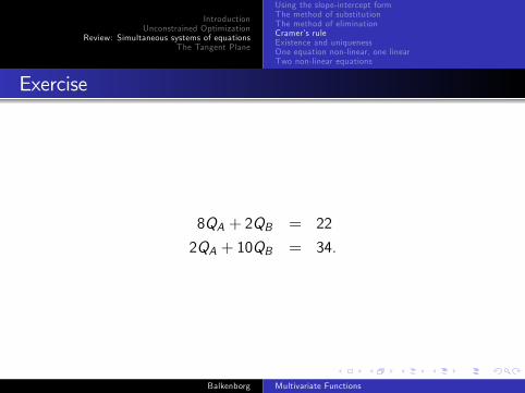
Exercise
8QA + 2QB = 22
2QA + 10QB = 34.
Balkenborg Multivariate Functions
IntroductionUnconstrained Optimization
Review: Simultaneous systems of equationsThe Tangent Plane
Using the slope-intercept formThe method of substitutionThe method of eliminationCramer�s ruleExistence and uniquenessOne equation non-linear, one linearTwo non-linear equations
Outline1 Introduction2 Unconstrained Optimization
The �rst order conditionsExample 1Example 2: Maximizing pro�tsExample 3: Price Discrimination
3 Review: Simultaneous systems of equationsUsing the slope-intercept formThe method of substitutionThe method of eliminationCramer�s ruleExistence and uniquenessOne equation non-linear, one linearTwo non-linear equations
4 The Tangent PlaneThe Total Di¤erentialThe slope of level curvesThe Chain Rule Balkenborg Multivariate Functions
IntroductionUnconstrained Optimization
Review: Simultaneous systems of equationsThe Tangent Plane
Using the slope-intercept formThe method of substitutionThe method of eliminationCramer�s ruleExistence and uniquenessOne equation non-linear, one linearTwo non-linear equations
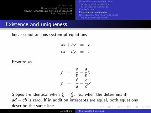
Existence and uniqueness
linear simultaneous system of equations
ax + by = e
cx + dy = f
Rewrite as
y =eb� abx
y =fd� cdx
Slopes are identical when ab =
cd , i.e., when the determinant
ad � cb is zero. If in addition intercepts are equal, both equationsdescribe the same line.
Balkenborg Multivariate Functions
IntroductionUnconstrained Optimization
Review: Simultaneous systems of equationsThe Tangent Plane
Using the slope-intercept formThe method of substitutionThe method of eliminationCramer�s ruleExistence and uniquenessOne equation non-linear, one linearTwo non-linear equations
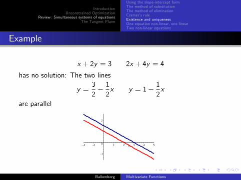
Example
x + 2y = 3 2x + 4y = 4
has no solution: The two lines
y =32� 12x y = 1� 1
2x
are parallel
1
0
2
2 1 1 2 3 4 5x
Balkenborg Multivariate Functions
IntroductionUnconstrained Optimization
Review: Simultaneous systems of equationsThe Tangent Plane
Using the slope-intercept formThe method of substitutionThe method of eliminationCramer�s ruleExistence and uniquenessOne equation non-linear, one linearTwo non-linear equations
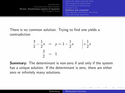
There is no common solution. Trying to �nd one yields acontradiction
32� 12x = y = 1� 1
2x
����+12x32= 1
Summary: The determinant is non-zero if and only if the systemhas a unique solution. If the determinant is zero, there are eitherzero or in�nitely many solutions.
Balkenborg Multivariate Functions
IntroductionUnconstrained Optimization
Review: Simultaneous systems of equationsThe Tangent Plane
Using the slope-intercept formThe method of substitutionThe method of eliminationCramer�s ruleExistence and uniquenessOne equation non-linear, one linearTwo non-linear equations
Outline1 Introduction2 Unconstrained Optimization
The �rst order conditionsExample 1Example 2: Maximizing pro�tsExample 3: Price Discrimination
3 Review: Simultaneous systems of equationsUsing the slope-intercept formThe method of substitutionThe method of eliminationCramer�s ruleExistence and uniquenessOne equation non-linear, one linearTwo non-linear equations
4 The Tangent PlaneThe Total Di¤erentialThe slope of level curvesThe Chain Rule Balkenborg Multivariate Functions
IntroductionUnconstrained Optimization
Review: Simultaneous systems of equationsThe Tangent Plane
Using the slope-intercept formThe method of substitutionThe method of eliminationCramer�s ruleExistence and uniquenessOne equation non-linear, one linearTwo non-linear equations
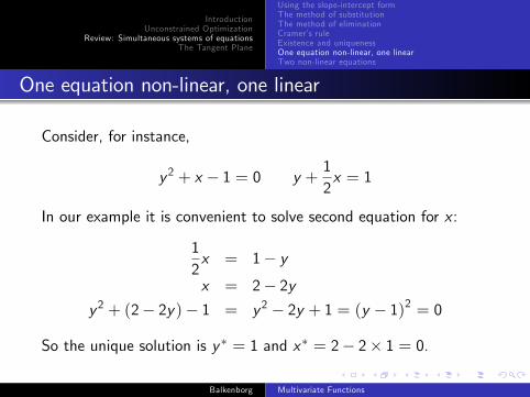
One equation non-linear, one linear
Consider, for instance,
y2 + x � 1 = 0 y +12x = 1
In our example it is convenient to solve second equation for x :
12x = 1� yx = 2� 2y
y2 + (2� 2y)� 1 = y2 � 2y + 1 = (y � 1)2 = 0
So the unique solution is y � = 1 and x� = 2� 2� 1 = 0.
Balkenborg Multivariate Functions
IntroductionUnconstrained Optimization
Review: Simultaneous systems of equationsThe Tangent Plane
Using the slope-intercept formThe method of substitutionThe method of eliminationCramer�s ruleExistence and uniquenessOne equation non-linear, one linearTwo non-linear equations
Outline1 Introduction2 Unconstrained Optimization
The �rst order conditionsExample 1Example 2: Maximizing pro�tsExample 3: Price Discrimination
3 Review: Simultaneous systems of equationsUsing the slope-intercept formThe method of substitutionThe method of eliminationCramer�s ruleExistence and uniquenessOne equation non-linear, one linearTwo non-linear equations
4 The Tangent PlaneThe Total Di¤erentialThe slope of level curvesThe Chain Rule Balkenborg Multivariate Functions
IntroductionUnconstrained Optimization
Review: Simultaneous systems of equationsThe Tangent Plane
Using the slope-intercept formThe method of substitutionThe method of eliminationCramer�s ruleExistence and uniquenessOne equation non-linear, one linearTwo non-linear equations
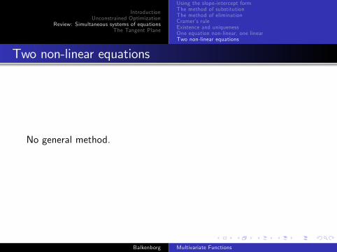
Two non-linear equations
No general method.
Balkenborg Multivariate Functions
IntroductionUnconstrained Optimization
Review: Simultaneous systems of equationsThe Tangent Plane
The Total Di¤erentialThe slope of level curvesThe Chain Rule
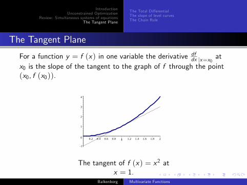
The Tangent Plane
For a function y = f (x) in one variable the derivative dfdx jx=x0 at
x0 is the slope of the tangent to the graph of f through the point(x0, f (x0)).
1
0
1
2
3
4
0 .2 0 .4 0 .6 0 .8 1 1 .2 1 .4 1 .6 1 .8 2x
The tangent of f (x) = x2 atx = 1.
Balkenborg Multivariate Functions
IntroductionUnconstrained Optimization
Review: Simultaneous systems of equationsThe Tangent Plane
The Total Di¤erentialThe slope of level curvesThe Chain Rule
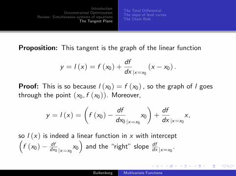
Proposition: This tangent is the graph of the linear function
y = l (x) = f (x0) +dfdx jx=x0
(x � x0) .
Proof: This is so because l (x0) = f (x0) , so the graph of l goesthrough the point (x0, f (x0)). Moreover,
y = l (x) =�f (x0)�
dfdx0 jx=x0
x0
�+dfdx jx=x0
x ,
so l (x) is indeed a linear function in x with intercept�f (x0)� df
dx0 jx=x0x0�and the �right� slope df
dx jx=x0 .
Balkenborg Multivariate Functions
IntroductionUnconstrained Optimization
Review: Simultaneous systems of equationsThe Tangent Plane
The Total Di¤erentialThe slope of level curvesThe Chain Rule
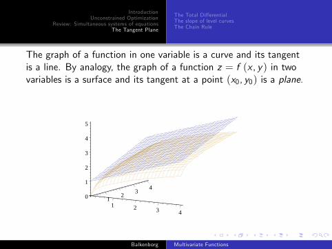
The graph of a function in one variable is a curve and its tangentis a line. By analogy, the graph of a function z = f (x , y) in twovariables is a surface and its tangent at a point (x0, y0) is a plane.
0
1
2
3
4
5
1 2 3 4
1 2 3 4
Balkenborg Multivariate Functions
IntroductionUnconstrained Optimization
Review: Simultaneous systems of equationsThe Tangent Plane
The Total Di¤erentialThe slope of level curvesThe Chain Rule
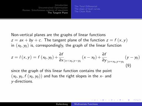
Non-vertical planes are the graphs of linear functionsz = ax + by + c . The tangent plane of the function z = f (x , y)in (x0, y0) is, correspondingly, the graph of the linear function
z = l (x , y) = f (x0, y0)+∂f∂x jx=x0,y=y0
(x � x0)+∂f∂y jx=x0,y=y0
(y � y0)
(9)since the graph of this linear function contains the point(x0, y0, f (x0, y0)) and has the right slopes in the x- andy -directions.
Balkenborg Multivariate Functions
IntroductionUnconstrained Optimization
Review: Simultaneous systems of equationsThe Tangent Plane
The Total Di¤erentialThe slope of level curvesThe Chain Rule
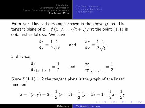
Exercise: This is the example shown in the above graph. Thetangent plane of z = f (x , y) =
px +
py at the point (1, 1) is
obtained as follows: We have
∂z∂x=121px
and∂z∂y=121py
and hence
∂z∂x jx=1,y=1
=12
and∂z∂y jx=1,y=1
=12.
Since f (1, 1) = 2 the tangent plane is the graph of the linearfunction
z = l (x , y) = 2+12(x � 1) + 1
2(y � 1) = 1+ 1
2x +
12y
Balkenborg Multivariate Functions
IntroductionUnconstrained Optimization
Review: Simultaneous systems of equationsThe Tangent Plane
The Total Di¤erentialThe slope of level curvesThe Chain Rule
Outline1 Introduction2 Unconstrained Optimization
The �rst order conditionsExample 1Example 2: Maximizing pro�tsExample 3: Price Discrimination
3 Review: Simultaneous systems of equationsUsing the slope-intercept formThe method of substitutionThe method of eliminationCramer�s ruleExistence and uniquenessOne equation non-linear, one linearTwo non-linear equations
4 The Tangent PlaneThe Total Di¤erentialThe slope of level curvesThe Chain Rule Balkenborg Multivariate Functions
IntroductionUnconstrained Optimization
Review: Simultaneous systems of equationsThe Tangent Plane
The Total Di¤erentialThe slope of level curvesThe Chain Rule
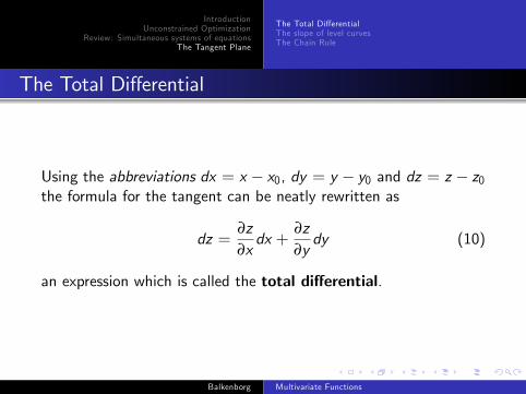
The Total Di¤erential
Using the abbreviations dx = x � x0, dy = y � y0 and dz = z � z0the formula for the tangent can be neatly rewritten as
dz =∂z∂xdx +
∂z∂ydy (10)
an expression which is called the total di¤erential.
Balkenborg Multivariate Functions
IntroductionUnconstrained Optimization
Review: Simultaneous systems of equationsThe Tangent Plane
The Total Di¤erentialThe slope of level curvesThe Chain Rule
Outline1 Introduction2 Unconstrained Optimization
The �rst order conditionsExample 1Example 2: Maximizing pro�tsExample 3: Price Discrimination
3 Review: Simultaneous systems of equationsUsing the slope-intercept formThe method of substitutionThe method of eliminationCramer�s ruleExistence and uniquenessOne equation non-linear, one linearTwo non-linear equations
4 The Tangent PlaneThe Total Di¤erentialThe slope of level curvesThe Chain Rule Balkenborg Multivariate Functions
IntroductionUnconstrained Optimization
Review: Simultaneous systems of equationsThe Tangent Plane
The Total Di¤erentialThe slope of level curvesThe Chain Rule
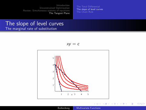
The slope of level curvesThe marginal rate of substitution
xy = c
1
2
3
4
5
1 2 3 4 5x
Balkenborg Multivariate Functions
IntroductionUnconstrained Optimization
Review: Simultaneous systems of equationsThe Tangent Plane
The Total Di¤erentialThe slope of level curvesThe Chain Rule
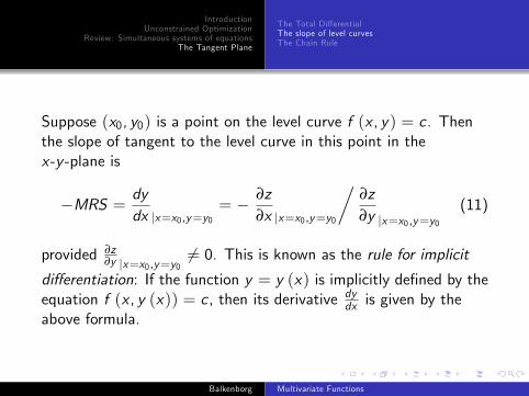
Suppose (x0, y0) is a point on the level curve f (x , y) = c . Thenthe slope of tangent to the level curve in this point in thex-y -plane is
�MRS = dydx jx=x0,y=y0
= � ∂z∂x jx=x0,y=y0
�∂z∂y jx=x0,y=y0
(11)
provided ∂z∂y jx=x0,y=y0
6= 0. This is known as the rule for implicitdi¤erentiation: If the function y = y (x) is implicitly de�ned by theequation f (x , y (x)) = c , then its derivative dy
dx is given by theabove formula.
Balkenborg Multivariate Functions
IntroductionUnconstrained Optimization
Review: Simultaneous systems of equationsThe Tangent Plane
The Total Di¤erentialThe slope of level curvesThe Chain Rule
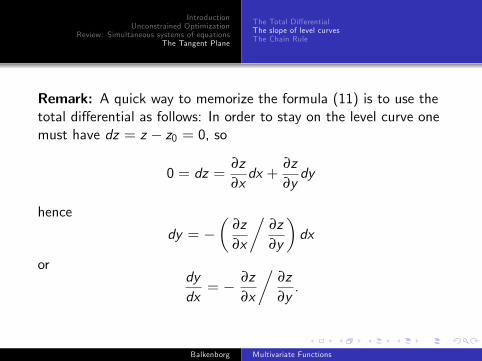
Remark: A quick way to memorize the formula (11) is to use thetotal di¤erential as follows: In order to stay on the level curve onemust have dz = z � z0 = 0, so
0 = dz =∂z∂xdx +
∂z∂ydy
hence
dy = ��
∂z∂x
�∂z∂y
�dx
ordydx= � ∂z
∂x
�∂z∂y.
Balkenborg Multivariate Functions
IntroductionUnconstrained Optimization
Review: Simultaneous systems of equationsThe Tangent Plane
The Total Di¤erentialThe slope of level curvesThe Chain Rule
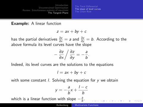
Example: A linear function
z = ax + by + c
has the partial derivatives ∂z∂x = a and
∂z∂y = b. According to the
above formula its level curves have the slope
� ∂z∂x
�∂z∂y= � a
b.
Indeed, its level curves are the solutions to the equations
l = ax + by + c
with some constant l . Solving the equation for y we obtain
y = � abx +
l � cb
which is a linear function with slope � ab .
Balkenborg Multivariate Functions
IntroductionUnconstrained Optimization
Review: Simultaneous systems of equationsThe Tangent Plane
The Total Di¤erentialThe slope of level curvesThe Chain Rule
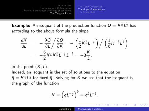
Example: An isoquant of the production function Q = K16 L
12 has
according to the above formula the slope
dKdL
= � ∂Q∂L
�∂Q∂K
= ��12K
16 L�
12
���16K�
56 L
12
�= �6
2K
16K
56 L�
12 L�
12 = �3K
L.
in the point (K , L).Indeed, an isoquant is the set of solutions to the equationq̄ = K
16 L
12 for �xed q̄. Solving for K we see that the isoquant is
the graph of the function
K =�q̄L�
12
�6= q̄6L�3.
Balkenborg Multivariate Functions
IntroductionUnconstrained Optimization
Review: Simultaneous systems of equationsThe Tangent Plane
The Total Di¤erentialThe slope of level curvesThe Chain Rule
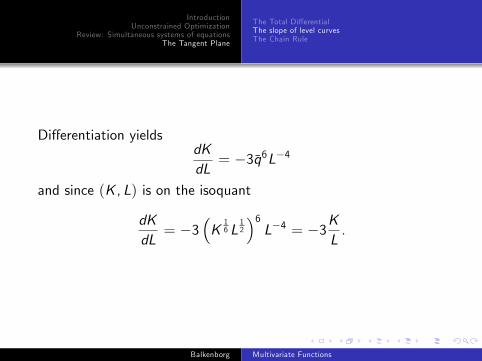
Di¤erentiation yieldsdKdL
= �3q̄6L�4
and since (K , L) is on the isoquant
dKdL
= �3�K
16 L
12
�6L�4 = �3K
L.
Balkenborg Multivariate Functions
IntroductionUnconstrained Optimization
Review: Simultaneous systems of equationsThe Tangent Plane
The Total Di¤erentialThe slope of level curvesThe Chain Rule
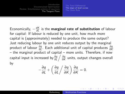
Economically, � dKdL is the marginal rate of substitution of labour
for capital: If labour is reduced by one unit, how much morecapital is (approximately) needed to produce the same output?Just reducing labour by one unit reduces output by the marginalproduct of labour ∂q
∂L . Each additional unit of capital produces∂q∂K
�the marginal product of capital �more units. Therefore, if nowcapital input is increased by ∂q
∂L
.∂q∂K units, output changes overall
by
�∂q∂L+
�∂q∂L
�∂q∂K
�∂q∂K
= 0.
Balkenborg Multivariate Functions
IntroductionUnconstrained Optimization
Review: Simultaneous systems of equationsThe Tangent Plane
The Total Di¤erentialThe slope of level curvesThe Chain Rule
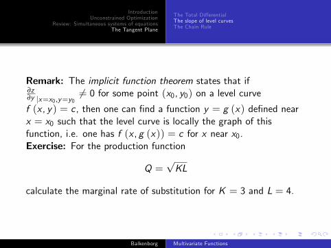
Remark: The implicit function theorem states that if∂z∂y jx=x0,y=y0
6= 0 for some point (x0, y0) on a level curvef (x , y) = c , then one can �nd a function y = g (x) de�ned nearx = x0 such that the level curve is locally the graph of thisfunction, i.e. one has f (x , g (x)) = c for x near x0.Exercise: For the production function
Q =pKL
calculate the marginal rate of substitution for K = 3 and L = 4.
Balkenborg Multivariate Functions
IntroductionUnconstrained Optimization
Review: Simultaneous systems of equationsThe Tangent Plane
The Total Di¤erentialThe slope of level curvesThe Chain Rule
Outline1 Introduction2 Unconstrained Optimization
The �rst order conditionsExample 1Example 2: Maximizing pro�tsExample 3: Price Discrimination
3 Review: Simultaneous systems of equationsUsing the slope-intercept formThe method of substitutionThe method of eliminationCramer�s ruleExistence and uniquenessOne equation non-linear, one linearTwo non-linear equations
4 The Tangent PlaneThe Total Di¤erentialThe slope of level curvesThe Chain Rule Balkenborg Multivariate Functions
IntroductionUnconstrained Optimization
Review: Simultaneous systems of equationsThe Tangent Plane
The Total Di¤erentialThe slope of level curvesThe Chain Rule
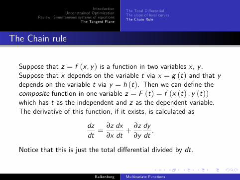
The Chain rule
Suppose that z = f (x , y) is a function in two variables x , y .Suppose that x depends on the variable t via x = g (t) and that ydepends on the variable t via y = h (t). Then we can de�ne thecomposite function in one variable z = F (t) = f (x (t) , y (t))which has t as the independent and z as the dependent variable.The derivative of this function, if it exists, is calculated as
dzdt=
∂z∂xdxdt+
∂z∂ydydt.
Notice that this is just the total di¤erential divided by dt.
Balkenborg Multivariate Functions
IntroductionUnconstrained Optimization
Review: Simultaneous systems of equationsThe Tangent Plane
The Total Di¤erentialThe slope of level curvesThe Chain Rule
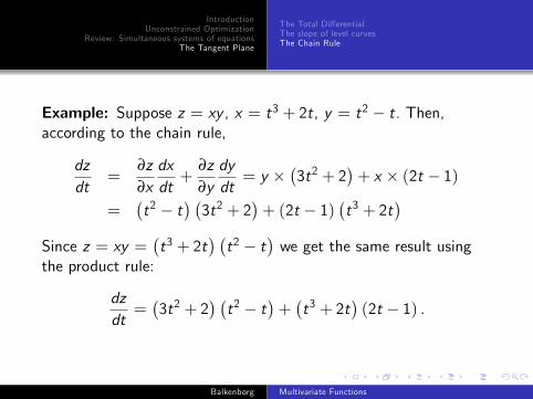
Example: Suppose z = xy , x = t3 + 2t, y = t2 � t. Then,according to the chain rule,
dzdt
=∂z∂xdxdt+
∂z∂ydydt= y �
�3t2 + 2
�+ x � (2t � 1)
=�t2 � t
� �3t2 + 2
�+ (2t � 1)
�t3 + 2t
�Since z = xy =
�t3 + 2t
� �t2 � t
�we get the same result using
the product rule:
dzdt=�3t2 + 2
� �t2 � t
�+�t3 + 2t
�(2t � 1) .
Balkenborg Multivariate Functions