BEC  

HANDOUT

2011

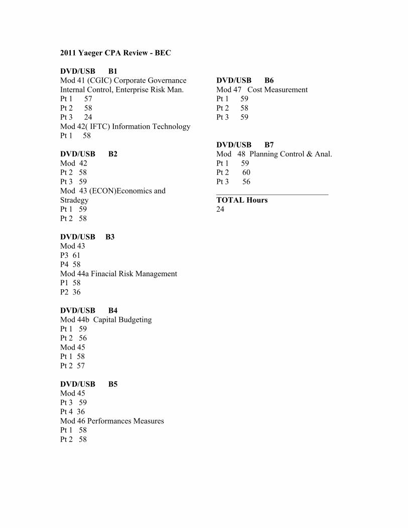
2011 Yaeger CPA Review - BEC DVD/USB B1 Mod 41 (CGIC) Corporate Governance Internal Control, Enterprise Risk Man. Pt 1 57 Pt 2 58 Pt 3 24 Mod 42( IFTC) Information Technology Pt 1 58 DVD/USB B2 Mod 42 Pt 2 58 Pt 3 59 Mod 43 (ECON)Economics and Stradegy Pt 1 59 Pt 2 58 DVD/USB B3 Mod 43 P3 61 P4 58 Mod 44a Finacial Risk Management P1 58 P2 36 DVD/USB B4 Mod 44b Capital Budgeting Pt 1 59 Pt 2 56 Mod 45 Pt 1 58 Pt 2 57 DVD/USB B5 Mod 45 Pt 3 59 Pt 4 36 Mod 46 Performances Measures Pt 1 58 Pt 2 58

DVD/USB B6 Mod 47 Cost Measurement Pt 1 59 Pt 2 58 Pt 3 59 DVD/USB B7 Mod 48 Planning Control & Anal. Pt 1 59 Pt 2 60 Pt 3 56 ____________________________ TOTAL Hours 24

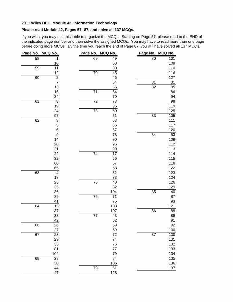
2011 Wiley BEC, Module 42, Information Technology

Please read Module 42, Pages 57--87, and solve all 137 MCQs.

If you wish, you may use this table to organize the MCQs. Starting on Page 57, please read to the END ofthe indicated page number and then solve the assigned MCQs. You may have to read more than one page before doing more MCQs. By the time you reach the end of Page 87, you will have solved all 137 MCQs.

Page No. MCQ No. Page No. MCQ No. Page No. MCQ No.

58 1 69 49 80 10110 68 109

59 11 80 11012 70 45 116

60 2 46 1277 54 81 31

13 55 82 8516 71 64 8634 70 94

61 8 72 73 9819 95 11924 73 50 12597 61 83 105

62 3 63 1115 66 1176 67 1209 78 84 53

14 90 10820 96 11221 99 11322 74 17 11432 56 11560 57 11865 58 122

63 4 62 12318 83 12425 75 48 12635 82 12936 104 85 4039 76 71 8741 75 93

64 15 103 12137 107 86 8838 77 43 8942 52 91

66 26 59 9227 69 100

67 28 72 87 13029 74 13133 76 13281 77 133

102 79 13468 23 84 135

30 106 13644 79 51 13747 128

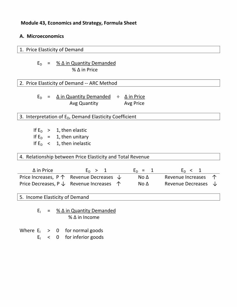
 Module 43, Economics and Strategy, Formula Sheet  A.  Microeconomics  

1.  Price Elasticity of Demand 

      ED  =     % Δ in Quantity Demanded                         % Δ in Price  

2.  Price Elasticity of Demand ‐‐ ARC Method 

      ED  =     Δ in Quantity Demanded     ÷    Δ in Price                             Avg Quantity                   Avg Price  

3.  Interpretation of ED, Demand Elasticity Coefficient 

   If ED  >     1, then elastic   If ED  =     1, then unitary   If ED  <     1, then inelastic  

4.  Relationship between Price Elasticity and Total Revenue 

 Δ in Price  ED      >     1  ED     =     1  ED     <     1 

Price Increases,  P ↑  Revenue Decreases   ↓ No Δ  Revenue Increases     ↑ Price Decreases, P ↓   Revenue Increases    ↑  No Δ  Revenue Decreases    ↓ 

5.  Income Elasticity of Demand 

      EI  =     % Δ in Quantity Demanded                      % Δ in Income  Where  EI  >     0     for normal goods      EI  <     0     for inferior goods 

6.  Cross Elasticity of Demand      (The Δ in Quantity demanded for X versus the Δ in Price for Y) 

      EXY  =      % Δ in Quantity Demanded of X                           % Δ in Price of Y  Where  EXY  >     0     for substitutes      EXY  =     0     for unrelated goods      EXY  <     0     for complements  

7.  Consumption Function 

      C  =     c0     +     c1YD  Where  C  =     Consumption for the period      YD  =     Disposable income for the period      c0  =     The constant      c1  =     The slope of the consumption function And     c1  =     MPC, the marginal propensity to consume  

8.  Relationship between Marginal Propensity to Save (MPS) and       Marginal Propensity to Consume (MPC) 

    MPS   +   MPC  =  1  

9.  Elasticity of Supply 

      ES  =     % Δ in Quantity Supplied                       % Δ in Price  

9A.  Interpretation of ES, Supply Elasticity Coefficient 

   If ES  >     1, then elastic   If ES  =     1, then unitary   If ES  <     1, then inelastic  

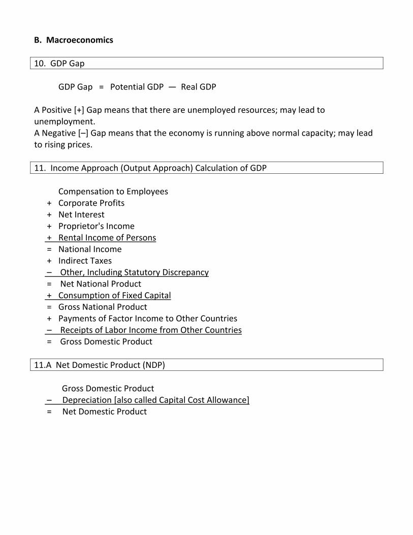
B.  Macroeconomics  

10.  GDP Gap 

   GDP Gap   =   Potential GDP  —  Real GDP  A Positive [+] Gap means that there are unemployed resources; may lead to unemployment. A Negative [–] Gap means that the economy is running above normal capacity; may lead to rising prices.  

11.  Income Approach (Output Approach) Calculation of GDP 

   Compensation to Employees       +  Corporate Profits       +  Net Interest       +  Proprietor's Income       +  Rental Income of Persons       =  National Income       +  Indirect Taxes       –    Other, Including Statutory Discrepancy       =    Net National Product       +  Consumption of Fixed Capital       =  Gross National Product       +  Payments of Factor Income to Other Countries       –    Receipts of Labor Income from Other Countries       =    Gross Domestic Product  

11.A  Net Domestic Product (NDP) 

              Gross Domestic Product       –     Depreciation [also called Capital Cost Allowance]       =     Net Domestic Product 

 

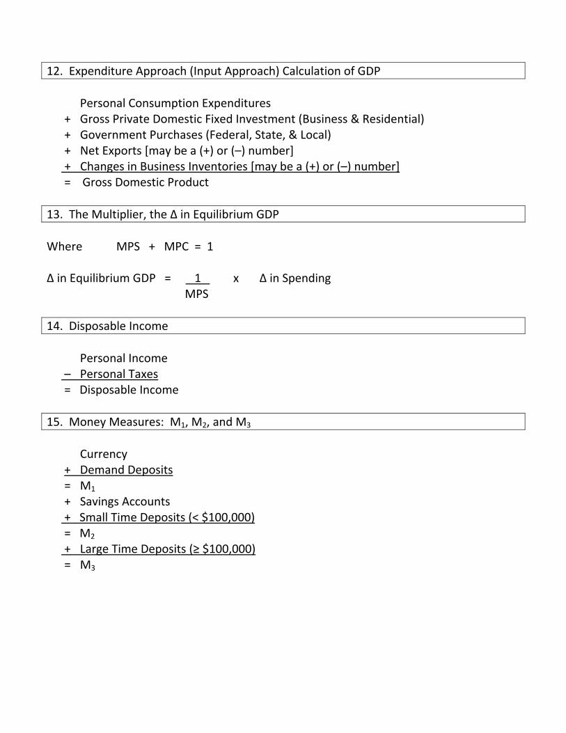
12.  Expenditure Approach (Input Approach) Calculation of GDP 

   Personal Consumption Expenditures       +  Gross Private Domestic Fixed Investment (Business & Residential)       +  Government Purchases (Federal, State, & Local)       +  Net Exports [may be a (+) or (–) number]       +  Changes in Business Inventories [may be a (+) or (–) number]       =    Gross Domestic Product  

13.  The Multiplier, the Δ in Equilibrium GDP 

 Where   MPS   +   MPC  =  1  Δ in Equilibrium GDP   =        1           x       Δ in Spending                      MPS  

14.  Disposable Income 

        Personal Income       –  Personal Taxes              =   Disposable Income  

15.  Money Measures:  M1, M2, and M3 

   Currency       +  Demand Deposits       =  M1       +  Savings Accounts       +   Small Time Deposits (< $100,000)       =   M2 

      +  Large Time Deposits (≥ $100,000)       =  M3 

 

     

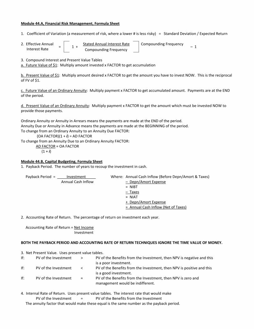
Module 44.A, Financial Risk Management, Formula Sheet  1.   Coefficient of Variation (a measurement of risk, where a lower # is less risky)   =   Standard Deviation / Expected Return  

Stated Annual Interest Rate    Compounding Frequency   2.  Effective Annual       Interest Rate 

=    1  +    Compounding Frequency     

  –  1  

 3.  Compound Interest and Present Value Tables a.  Future Value of $1:  Multiply amount invested x FACTOR to get accumulation  b.  Present Value of $1:  Multiply amount desired x FACTOR to get the amount you have to invest NOW.  This is the reciprocal of FV of $1.  c.  Future Value of an Ordinary Annuity:  Multiply payment x FACTOR to get accumulated amount.  Payments are at the END of the period.  d.  Present Value of an Ordinary Annuity:  Multiply payment x FACTOR to get the amount which must be invested NOW to provide those payments.  Ordinary Annuity or Annuity in Arrears means the payments are made at the END of the period. Annuity Due or Annuity in Advance means the payments are made at the BEGINNING of the period. To change from an Ordinary Annuity to an Annuity Due FACTOR: 

 (OA FACTOR)(1 + i) = AD FACTOR To change from an Annuity Due to an Ordinary Annuity FACTOR: 

AD FACTOR = OA FACTOR       (1 + i)  

Module 44.B, Capital Budgeting, Formula Sheet 1.  Payback Period.  The number of years to recoup the investment in cash.       Payback Period  =            Investment    Where:  Annual Cash Inflow (Before Depn/Amort & Taxes)                    Annual Cash Inflow      –  Depn/Amort Expense               =  NIBT               –  Taxes                =  NIAT               +  Depn/Amort Expense               =  Annual Cash Inflow (Net of Taxes)  2.  Accounting Rate of Return.  The percentage of return on investment each year.       Accounting Rate of Return = Net Income 

         Investment  BOTH THE PAYBACK PERIOD AND ACCOUNTING RATE OF RETURN TECHNIQUES IGNORE THE TIME VALUE OF MONEY.  3.  Net Present Value.  Uses present value tables. If:  PV of the Investment  >  PV of the Benefits from the Investment, then NPV is negative and this              is a poor investment. If:  PV of the Investment   <  PV of the Benefits from the Investment, then NPV is positive and this              is a good investment. If:  PV of the Investment  =  PV of the Benefits from the Investment, then NPV is zero and               management would be indifferent.  4.  Internal Rate of Return.  Uses present value tables.  The interest rate that would make 

PV of the Investment   =  PV of the Benefits from the Investment      The annuity factor that would make these equal is the same number as the payback period. 

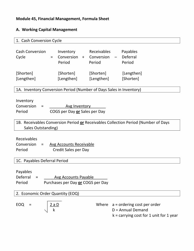
Module 45, Financial Management, Formula Sheet  A.  Working Capital Management  

1.  Cash Conversion Cycle 

 Cash Conversion            Inventory              Receivables           Payables Cycle                         =     Conversion    +     Conversion     –     Deferral                                           Period                   Period                     Period  [Shorten]                         [Shorten]              [Shorten]                [Lengthen] [Lengthen]                      [Lengthen]            [Lengthen]             [Shorten]    

1A.  Inventory Conversion Period (Number of Days Sales in Inventory) 

 Inventory Conversion     =                      Avg Inventory                                           Period             COGS per Day or Sales per Day  

1B.  Receivables Conversion Period or Receivables Collection Period (Number of Days         Sales Outstanding) 

 Receivables Conversion     =      Avg Accounts Receivable       Period                Credit Sales per Day  

1C.  Payables Deferral Period 

 Payables Deferral     =            Avg Accounts Payable                Period       Purchases per Day or COGS per Day  

2.  Economic Order Quantity (EOQ) 

 EOQ     =              2 a D        Where    a = ordering cost per order                   k                        D = Annual Demand                      k = carrying cost for 1 unit for 1 year 

 

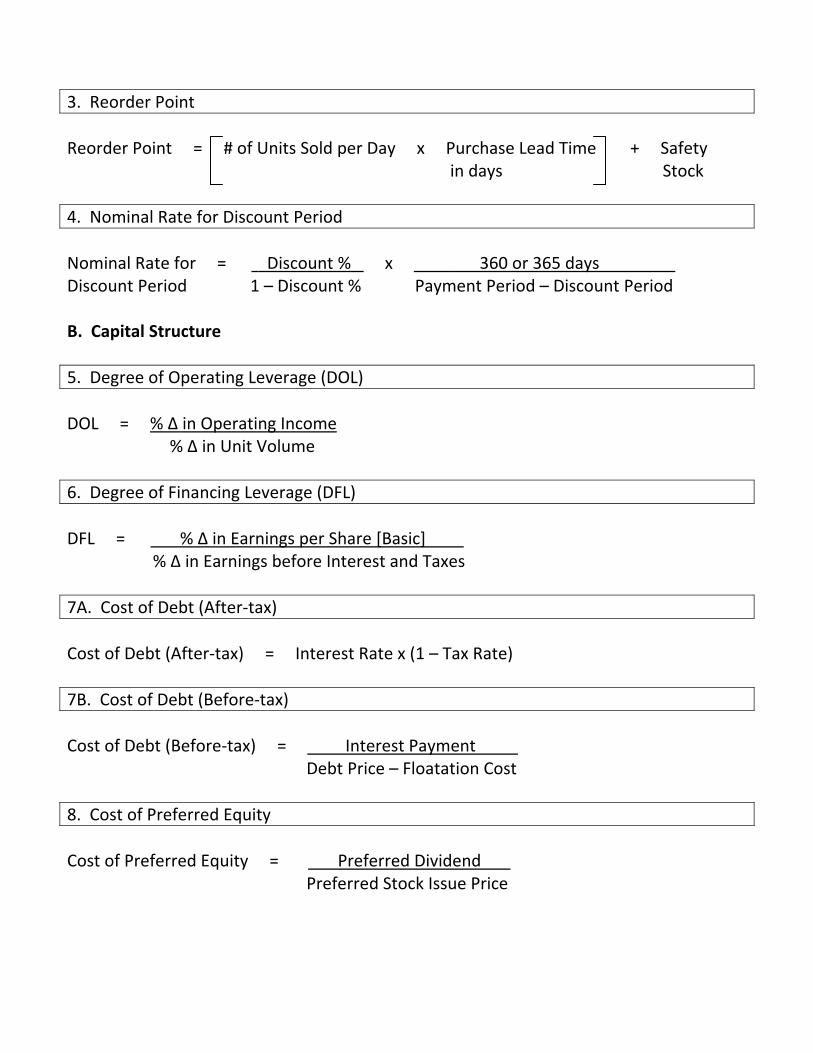
3.  Reorder Point 

 Reorder Point     =     # of Units Sold per Day     x     Purchase Lead Time        +     Safety                                                                                            in days                                      Stock  

4.  Nominal Rate for Discount Period 

 Nominal Rate for     =          Discount %        x              360 or 365 days              Discount Period               1 – Discount %     Payment Period – Discount Period  B.  Capital Structure  

5.  Degree of Operating Leverage (DOL) 

 DOL     =     % Δ in Operating Income                                                                                          % Δ in Unit Volume  

6.  Degree of Financing Leverage (DFL) 

 DFL     =             % Δ in Earnings per Share [Basic]                                                                                                  % Δ in Earnings before Interest and Taxes  

7A.  Cost of Debt (After‐tax) 

 Cost of Debt (After‐tax)     =     Interest Rate x (1 – Tax Rate)                                  

7B.  Cost of Debt (Before‐tax) 

 Cost of Debt (Before‐tax)     =              Interest Payment                                                     Debt Price – Floatation Cost      

8.  Cost of Preferred Equity 

 Cost of Preferred Equity     =              Preferred Dividend                              Preferred Stock Issue Price 

 

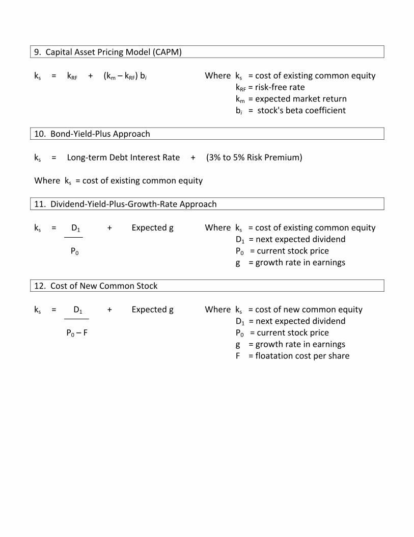
9.  Capital Asset Pricing Model (CAPM) 

 ks     =     kRF     +     (km – kRF) bi       Where  ks   = cost of existing common equity                    kRF = risk‐free rate                    km  = expected market return                    bi   =  stock's beta coefficient  

10.  Bond‐Yield‐Plus Approach 

 ks     =     Long‐term Debt Interest Rate     +     (3% to 5% Risk Premium)  Where  ks  = cost of existing common equity  

11.  Dividend‐Yield‐Plus‐Growth‐Rate Approach 

 ks     =       D1   +  Expected g    Where  ks   = cost of existing common equity                    D1  = next expected dividend                        P0                    P0   = current stock price                    g    = growth rate in earnings  

12.  Cost of New Common Stock 

 ks     =        D1   +  Expected g    Where  ks   = cost of new common equity                    D1  = next expected dividend                      P0 – F               P0   = current stock price                    g    = growth rate in earnings                    F    = floatation cost per share 

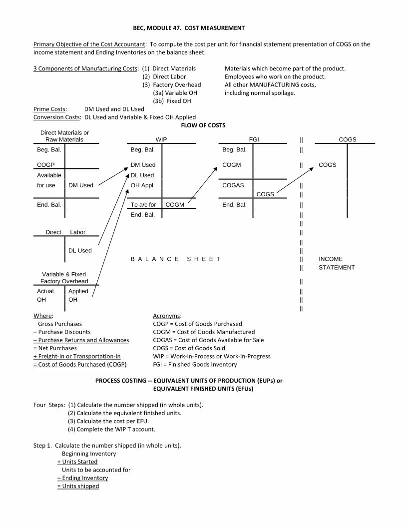
BEC, MODULE 47.  COST MEASUREMENT  Primary Objective of the Cost Accountant:  To compute the cost per unit for financial statement presentation of COGS on the income statement and Ending Inventories on the balance sheet.  3 Components of Manufacturing Costs:  (1)  Direct Materials    Materials which become part of the product. 

         (2)  Direct Labor    Employees who work on the product.          (3)  Factory Overhead  All other MANUFACTURING costs,   (3a) Variable OH    including normal spoilage.   (3b)  Fixed OH 

Prime Costs:     DM Used and DL Used Conversion Costs:  DL Used and Variable & Fixed OH Applied 

FLOW OF COSTS  Direct Materials or Raw Materials WIP FGI || COGS

Beg. Bal. Beg. Bal. Beg. Bal. ||

COGP DM Used

COGM

|| COGS

Available DL Used

for use DM Used OH Appl COGAS ||

COGS ||

End. Bal. To a/c for COGM End. Bal. ||

End. Bal. ||

||

Direct Labor ||

||

DL Used ||

B A L A N C E S H E E T || INCOME

|| STATEMENT Variable & Fixed Factory Overhead ||

Actual Applied ||

OH OH ||

|| Where:          Acronyms:      Gross Purchases      COGP = Cost of Goods Purchased – Purchase Discounts      COGM = Cost of Goods Manufactured – Purchase Returns and Allowances  COGAS = Cost of Goods Available for Sale = Net Purchases        COGS = Cost of Goods Sold + Freight‐In or Transportation‐in    WIP = Work‐in‐Process or Work‐in‐Progress = Cost of Goods Purchased (COGP)    FGI = Finished Goods Inventory    PROCESS COSTING ‐‐ EQUIVALENT UNITS OF PRODUCTION (EUPs) or 

EQUIVALENT FINISHED UNITS (EFUs)  Four  Steps:  (1) Calculate the number shipped (in whole units). 

       (2) Calculate the equivalent finished units.        (3) Calculate the cost per EFU.        (4) Complete the WIP T account. 

 Step 1.  Calculate the number shipped (in whole units). 

   Beginning Inventory + Units Started                      Units to be accounted for – Ending Inventory            = Units shipped                  

MODULE 47.  PROCESS COSTING ‐‐ EUPs or EFUs (Continued)  Step 2.  Calculate the equivalent finished units. A.  FIFO            B. Weighted‐Average 

                       DM              CC                  DM              CC         Units shipped             Units shipped + End. Inv. (EFUs)         + End. Inv. (EFUs)      – Beg. Inv. (EFUs)         = W/A EFUs           = FIFO EFUs           Step 3.  Calculate the cost per EFU A.  FIFO            B. Weighted‐Average Cost per EFU = Current Costs Only      Cost per EFU = Beg. Inv. + Current Costs 

        EFUs            EFUs  Step 4.  Complete the WIP T account.  Using the number of Ending Inventory EFUs from Step 2 and Cost per EFU in Step 3, calculate the $ value of ending inventory in WIP and plug COGM.  Lost Units: (1) Abnormal Spoilage is a PERIOD COST; do not include it in WIP. 

(2) Normal Spoilage is a PRODUCT COST; the costs of all units are spread over the good units; usually       part of OH. 

 BEC, MODULE 47.  COST MEASUREMENT 

BACKFLUSH COSTING  Traditional Cost Flows  Direct Materials             |             |    Direct Labor             WIP                FGI               COGS                                     |               |               |               |             |               |    COGM             |    COGS           |  Var & Fixed OH             |               |               |             |             |  Backflush Costing Method I ‐‐ JIT Inventory Methods with Vendors/Suppliers: Combine DM and WIP, Combine DL and OH  

      Materials & In‐Process          |            FGI                 COGS                      |               |                | 

     Conversion Cost Control           |                |            |               |                |          | 

 Backflush Costing Method II ‐‐ JIT Inventory Methods with Vendors/Suppliers & Customers: Same as Method I, but also no FGI. 

      Materials & In‐Process           |                  COGS    

         |                               |      Conversion Cost Control                        |   

         |                            |          |   

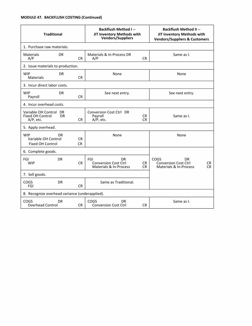
MODULE 47.  BACKFLUSH COSTING (Continued)   

 Traditional 

   Backflush Method I ‐‐ 

JIT Inventory Methods with Vendors/Suppliers 

   Backflush Method II ‐‐ 

JIT Inventory Methods with Vendors/Suppliers & Customers 

 1.  Purchase raw materials.  Materials                     DR      A/P  CR 

 Materials & In‐Process DR      A/P  CR 

   Same as I. 

 2.  Issue materials to production.  WIP                               DR      Materials  CR 

   None 

   None 

 3.  Incur direct labor costs.  WIP                               DR      Payroll  CR 

   See next entry. 

   See next entry. 

 4.  Incur overhead costs.  Variable OH Control   DR Fixed OH Control         DR      A/P, etc.  CR 

 Conversion Cost Ctrl   DR      Payroll  CR     A/P, etc.  CR 

    Same as I. 

 5.  Apply overhead.  WIP                              DR      Variable OH Control  CR       Fixed OH Control                      CR 

   None  

   None 

 6.  Complete goods. 

 

 FGI                               DR      WIP  CR 

 FGI                              DR      Conversion Cost Ctrl  CR     Materials & In‐Process  CR 

 COGS                         DR      Conversion Cost Ctrl  CR     Materials & In‐Process  CR 

 7.  Sell goods. 

  

 COGS                           DR      FGI  CR 

   Same as Traditional. 

  

 8.  Recognize overhead variance (underapplied).  COGS                           DR      Overhead Control  CR 

 COGS                          DR      Conversion Cost Ctrl  CR 

   Same as I. 

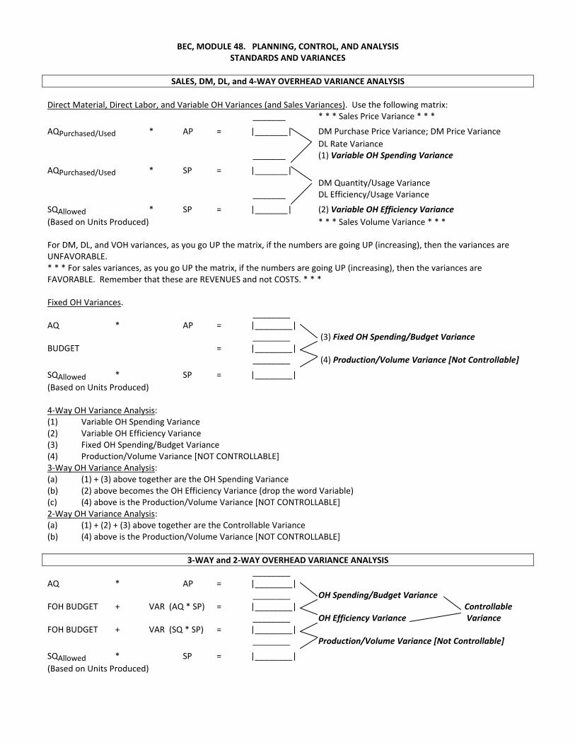
BEC, MODULE 48.   PLANNING, CONTROL, AND ANALYSIS STANDARDS AND VARIANCES 

 

SALES, DM, DL, and 4‐WAY OVERHEAD VARIANCE ANALYSIS 

 Direct Material, Direct Labor, and Variable OH Variances (and Sales Variances).  Use the following matrix: 

 _______  * * * Sales Price Variance * * * 

AQPurchased/Used  *  AP  =  |_______|  DM Purchase Price Variance; DM Price Variance   

    DL Rate Variance  _______  (1) Variable OH Spending Variance 

AQPurchased/Used  *  SP  =  |_______|   

DM Quantity/Usage Variance  _______  DL Efficiency/Usage Variance 

SQAllowed    *  SP  =  |_______|  (2) Variable OH Efficiency Variance 

(Based on Units Produced)           * * * Sales Volume Variance * * *  For DM, DL, and VOH variances, as you go UP the matrix, if the numbers are going UP (increasing), then the variances are UNFAVORABLE. * * * For sales variances, as you go UP the matrix, if the numbers are going UP (increasing), then the variances are FAVORABLE.  Remember that these are REVENUES and not COSTS. * * *  Fixed OH Variances.              ________ AQ    *    AP  =  |________|              ________   (3) Fixed OH Spending/Budget Variance BUDGET         =  |________|              ________   (4) Production/Volume Variance [Not Controllable] 

SQAllowed  *    SP  =  |________|   

(Based on Units Produced)  4‐Way OH Variance Analysis: (1)  Variable OH Spending Variance (2)  Variable OH Efficiency Variance (3)  Fixed OH Spending/Budget Variance (4)  Production/Volume Variance [NOT CONTROLLABLE] 3‐Way OH Variance Analysis: (a)  (1) + (3) above together are the OH Spending Variance (b)  (2) above becomes the OH Efficiency Variance (drop the word Variable) (c)  (4) above is the Production/Volume Variance [NOT CONTROLLABLE] 2‐Way OH Variance Analysis: (a)  (1) + (2) + (3) above together are the Controllable Variance (b)  (4) above is the Production/Volume Variance [NOT CONTROLLABLE]  

3‐WAY and 2‐WAY OVERHEAD VARIANCE ANALYSIS 

             ________ AQ    *    AP  =  |________|              ________  OH Spending/Budget Variance FOH BUDGET  +  VAR  (AQ * SP)  =  |________|               Controllable              ________  OH Efficiency Variance          Variance   FOH BUDGET  +  VAR  (SQ * SP)  =  |________|              ________  Production/Volume Variance [Not Controllable] 

SQAllowed  *    SP  =  |________|   

(Based on Units Produced)  

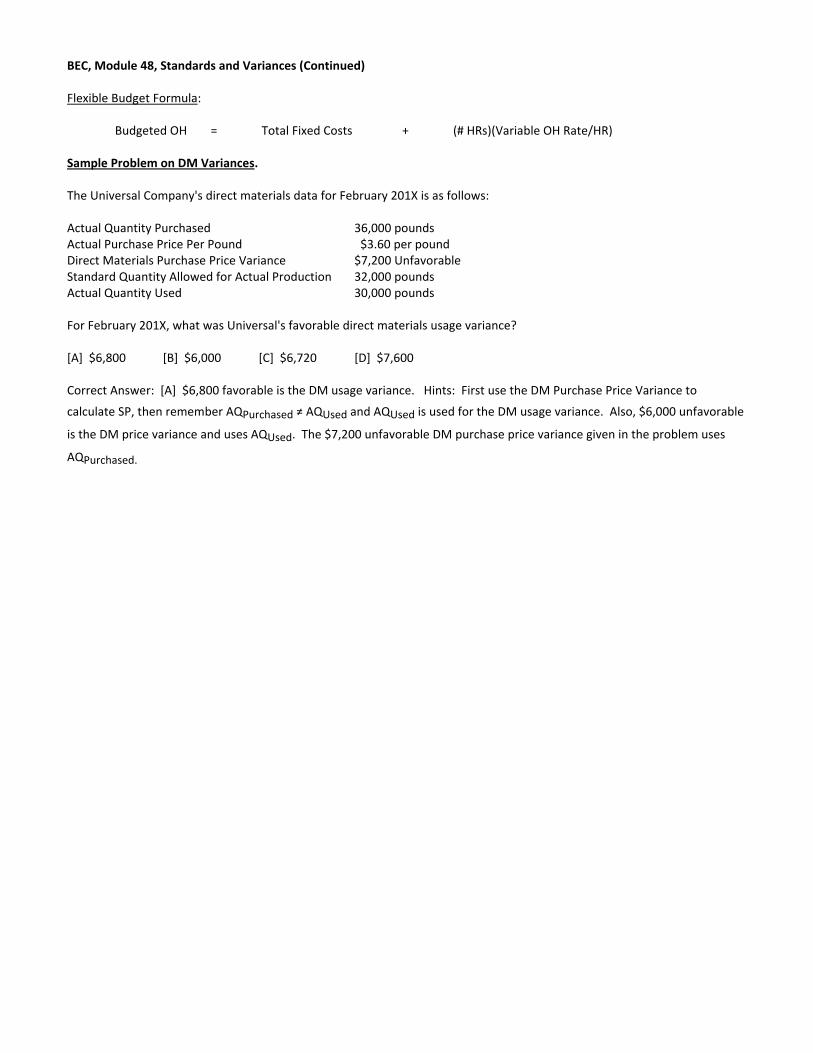
BEC, Module 48, Standards and Variances (Continued)  Flexible Budget Formula:   

Budgeted OH   =   Total Fixed Costs   +   (# HRs)(Variable OH Rate/HR)  Sample Problem on DM Variances.  The Universal Company's direct materials data for February 201X is as follows:   Actual Quantity Purchased      36,000 pounds Actual Purchase Price Per Pound        $3.60 per pound Direct Materials Purchase Price Variance     $7,200 Unfavorable Standard Quantity Allowed for Actual Production  32,000 pounds Actual Quantity Used        30,000 pounds  For February 201X, what was Universal's favorable direct materials usage variance?  [A]  $6,800  [B]  $6,000  [C]  $6,720  [D]  $7,600  Correct Answer:  [A]  $6,800 favorable is the DM usage variance.   Hints:  First use the DM Purchase Price Variance to 

calculate SP, then remember AQPurchased ≠ AQUsed and AQUsed is used for the DM usage variance.  Also, $6,000 unfavorable 

is the DM price variance and uses AQUsed.  The $7,200 unfavorable DM purchase price variance given in the problem uses 

AQPurchased. 

  

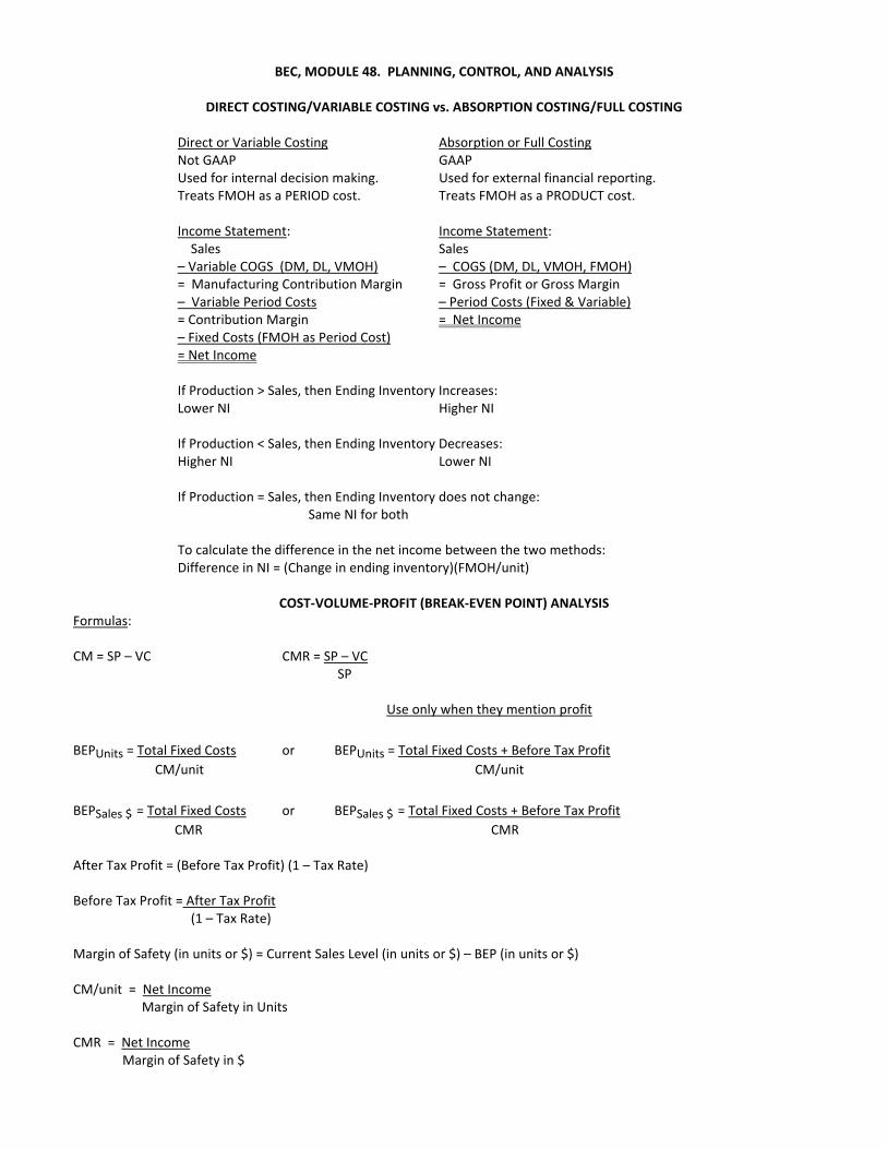
BEC, MODULE 48.  PLANNING, CONTROL, AND ANALYSIS  

DIRECT COSTING/VARIABLE COSTING vs. ABSORPTION COSTING/FULL COSTING  

Direct or Variable Costing      Absorption or Full Costing Not GAAP        GAAP Used for internal decision making.    Used for external financial reporting. Treats FMOH as a PERIOD cost.    Treats FMOH as a PRODUCT cost. 

 Income Statement:      Income Statement:     Sales               Sales – Variable COGS  (DM, DL, VMOH)     –  COGS (DM, DL, VMOH, FMOH)        =  Manufacturing Contribution Margin  =  Gross Profit or Gross Margin –  Variable Period Costs      – Period Costs (Fixed & Variable) = Contribution Margin      =  Net Income       – Fixed Costs (FMOH as Period Cost)    = Net Income                                         

 If Production > Sales, then Ending Inventory Increases: Lower NI        Higher NI 

 If Production < Sales, then Ending Inventory Decreases: Higher NI        Lower NI 

 If Production = Sales, then Ending Inventory does not change: 

        Same NI for both  

To calculate the difference in the net income between the two methods: Difference in NI = (Change in ending inventory)(FMOH/unit) 

 COST‐VOLUME‐PROFIT (BREAK‐EVEN POINT) ANALYSIS 

Formulas:  CM = SP – VC      CMR = SP – VC 

 SP  

Use only when they mention profit  

BEPUnits = Total Fixed Costs  or  BEPUnits = Total Fixed Costs + Before Tax Profit 

         CM/unit                     CM/unit  

BEPSales $ = Total Fixed Costs  or  BEPSales $ = Total Fixed Costs + Before Tax Profit                CMR            CMR 

 After Tax Profit = (Before Tax Profit) (1 – Tax Rate)  Before Tax Profit = After Tax Profit 

    (1 – Tax Rate)  

Margin of Safety (in units or $) = Current Sales Level (in units or $) – BEP (in units or $)  CM/unit  =  Net Income                                Margin of Safety in Units  CMR  =  Net Income                                      Margin of Safety in $

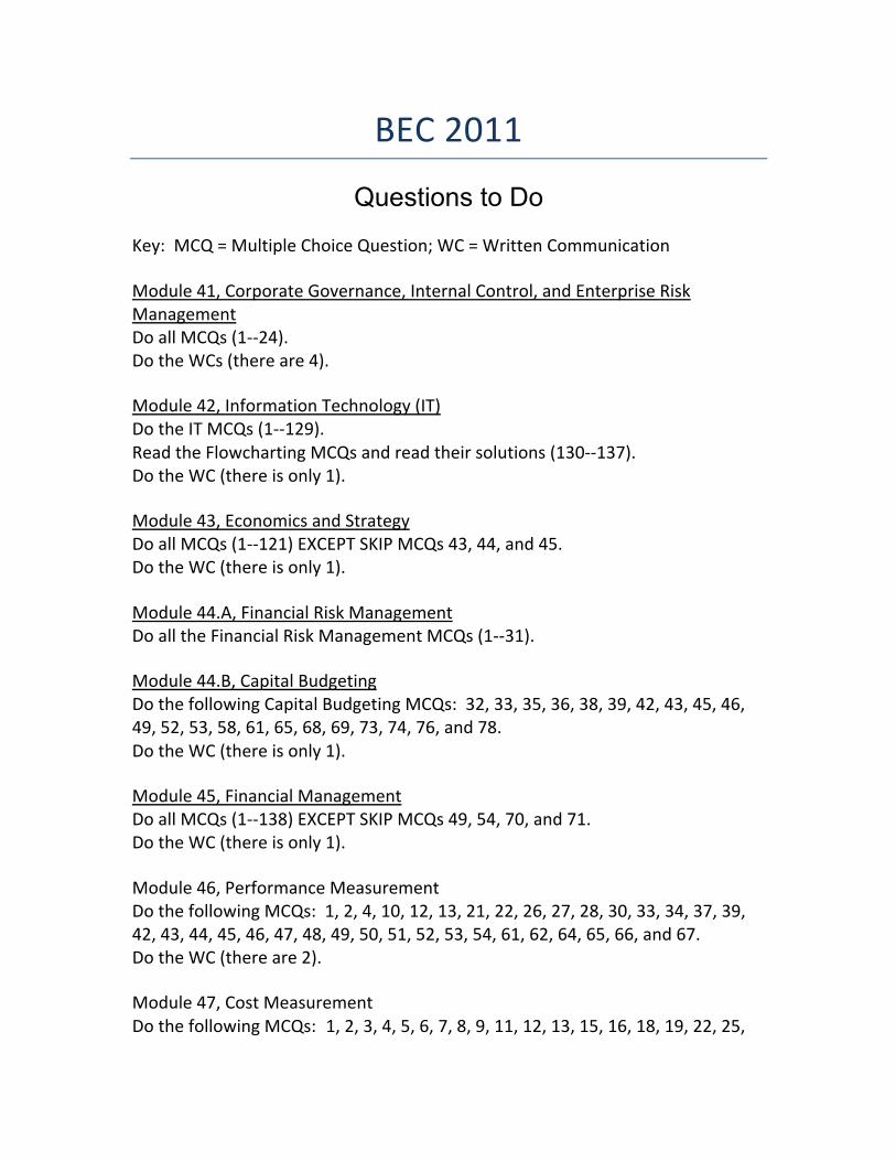
BEC  2011  

Questions to Do Key:    MCQ  =  Multiple  Choice  Question;  WC  =  Written  Communication Module  41,  Corporate  Governance,  Internal  Control,  and  Enterprise  Risk  Management   Do  all  MCQs  (1-­‐-­‐24). Do  the  WCs  (there  are  4). Module  42,  Information  Technology  (IT) Do  the  IT  MCQs  (1-­‐-­‐129). Read  the  Flowcharting  MCQs  and  read  their  solutions  (130-­‐-­‐137). Do  the  WC  (there  is  only  1). Module  43,  Economics  and  Strategy Do  all  MCQs  (1-­‐-­‐121)  EXCEPT  SKIP  MCQs  43,  44,  and  45. Do  the  WC  (there  is  only  1). Module  44.A,  Financial  Risk  Management Do  all  the  Financial  Risk  Management  MCQs  (1-­‐-­‐31). Module  44.B,  Capital  Budgeting Do  the  following  Capital  Budgeting  MCQs:    32,  33,  35,  36,  38,  39,  42,  43,  45,  46,  49,  52,  53,  58,  61,  65,  68,  69,  73,  74,  76,  and  78. Do  the  WC  (there  is  only  1). Module  45,  Financial  Management Do  all  MCQs  (1-­‐-­‐138)  EXCEPT  SKIP  MCQs  49,  54,  70,  and  71. Do  the  WC  (there  is  only  1). Module  46,  Performance  Measurement Do  the  following  MCQs:    1,  2,  4,  10,  12,  13,  21,  22,  26,  27,  28,  30,  33,  34,  37,  39,  42,  43,  44,  45,  46,  47,  48,  49,  50,  51,  52,  53,  54,  61,  62,  64,  65,  66,  and  67. Do  the  WC  (there  are  2). Module  47,  Cost  Measurement Do  the  following  MCQs:   1,  2,  3,  4,  5,  6,  7,  8,  9,  11,  12,  13,  15,  16,  18,  19,  22,  25,  

27,  29,  30,  31,  32,  33,  34,  35,  36,  37,  38,  39,  41,  42,  43,  44,  45,  47,  48,  49,  53,  54,  55,  56,  and  57. Do  the  WC  (there  is  only  1). Module  48,  Planning,  Control,  and  Analysis Do  the  following  MCQs:   1,  2,  3,  5,  6,  7,  8,  11,  13,  16,  17,  18,  19,  20,  2  1,  22,  23,  27,  28,  30,  32,  36,  37,  38,  43,  44,  45,  46,  47,  48,  49,  50,  51,  52,  53,  55,  56,  57,  58,  59,  63,  64,  66,  67,  70,  71,  72,  73,  74,  75,  76,  77,  79,  83,  84,  85,  86,  and  87.  Do  the  WC  (there  are  2).