Embed Size (px)
DESCRIPTION
statistical modelling
Citation preview

Latent Variable Modeling Using R
This step-by-step guide is written for R and latent variable model (LVM) novices. Utilizing apath model approach and focusing on the lavaan package, this book is designed to help readersquickly understand LVMs and their analysis in R. The author reviews the reasoning behind thesyntax selected and provides examples that demonstrate how to analyze data for a variety ofLVMs. Featuring examples applicable to psychology, education, business, and other social andhealth sciences, minimal text is devoted to theoretical underpinnings. The material is presentedwithout the use of matrix algebra. As a whole the book prepares readers to write about andinterpret LVM results they obtain in R.
Each chapter features background information, boldfaced key terms defined in the glossary,detailed interpretations of R output, descriptions of how to write the analysis of results forpublication, a summary, R based practice exercises (with solutions included in the back of thebook), and references and related readings. Margin notes help readers better understand LVMsand write their own R syntax. Examples using data from published work across a variety ofdisciplines demonstrate how to use R syntax for analyzing and interpreting results. R functions,syntax, and the corresponding results appear in gray boxes to help readers quickly locate thismaterial. A unique index helps readers quickly locate R functions, packages, and datasets. Thebook and accompanying website (http://blogs.baylor.edu/rlatentvariable) provide all of thedata for the book’s examples and exercises as well as R syntax so readers can replicate theanalyses. The book reviews how to enter the data into R, specify the LVMs, and obtain andinterpret the estimated parameter values.
Intended as a supplementary text for graduate and/or advanced undergraduate courses on latentvariable modeling, factor analysis, structural equation modeling, item response theory,measurement, or multivariate statistics taught in psychology, education, human development,business, economics, and social and health sciences, this book also appeals to researchers in thesefields. Prerequisites include familiarity with basic statistical concepts, but knowledge of R is notassumed.
A. Alexander Beaujean is an Associate Professor in Educational Psychology at BaylorUniversity.

This page intentionally left blank
Latent Variable Modeling Using RA Step-by-Step Guide
A. Alexander Beaujean

First published 2014by Routledge711 Third Avenue, New York, NY 10017
and by Routledge27 Church Road, Hove, East Sussex BN3 2FA
Routledge is an imprint of the Taylor & Francis Group, an informa business
© 2014 Taylor & Francis
The right of A. Alexander Beaujean to be identified as author of this work hasbeen asserted by him in accordance with sections 77 and 78 of the Copyright,Designs and Patents Act 1988.
All rights reserved. No part of this book may be reprinted or reproducedor utilised in any form or by any electronic, mechanical, or other means,now known or hereafter invented, including photocopying and recording,or in any information storage or retrieval system, without permission inwriting from the publishers.
Trademark notice: Product or corporate names may be trademarks orregistered trademarks, and are used only for identification and explanationwithout intent to infringe.
Library of Congress Cataloging in Publication DataA catalog record has been requested.
ISBN: 978-1-84872-698-7 (hbk)ISBN: 978-1-84872-699-4 (pbk)ISBN: 978-1-315-86978-0 (ebk)
Typeset in Latin Modern Romanby A. Alexander Beaujean
Contents
Author Biography viiPreface viii1 Introduction to R 1
1.1 Background . . . . . . . . . . . . . . . . . . . . . . . . . . . . . . . . . . . . . . . . 11.2 Hints for Using R . . . . . . . . . . . . . . . . . . . . . . . . . . . . . . . . . . . . . 181.3 Summary . . . . . . . . . . . . . . . . . . . . . . . . . . . . . . . . . . . . . . . . . 181.4 Exercises . . . . . . . . . . . . . . . . . . . . . . . . . . . . . . . . . . . . . . . . . . 181.5 References & Further Readings . . . . . . . . . . . . . . . . . . . . . . . . . . . . . . 20
2 Path Models and Analysis 212.1 Background . . . . . . . . . . . . . . . . . . . . . . . . . . . . . . . . . . . . . . . . 212.2 Using R For Path Analysis . . . . . . . . . . . . . . . . . . . . . . . . . . . . . . . . 272.3 Example: Path Analysis using lavaan . . . . . . . . . . . . . . . . . . . . . . . . . . 292.4 Indirect Effect . . . . . . . . . . . . . . . . . . . . . . . . . . . . . . . . . . . . . . . 302.5 Summary . . . . . . . . . . . . . . . . . . . . . . . . . . . . . . . . . . . . . . . . . 322.6 Writing the Results . . . . . . . . . . . . . . . . . . . . . . . . . . . . . . . . . . . . 322.7 Exercises . . . . . . . . . . . . . . . . . . . . . . . . . . . . . . . . . . . . . . . . . . 342.8 References & Further Readings . . . . . . . . . . . . . . . . . . . . . . . . . . . . . . 36
3 Basic Latent Variable Models 373.1 Background . . . . . . . . . . . . . . . . . . . . . . . . . . . . . . . . . . . . . . . . 373.2 Latent Variable Models . . . . . . . . . . . . . . . . . . . . . . . . . . . . . . . . . . 383.3 Example: Latent Variable Model with One Latent Variable . . . . . . . . . . . . . . 423.4 Example: Structural Equation Model . . . . . . . . . . . . . . . . . . . . . . . . . . 503.5 Summary . . . . . . . . . . . . . . . . . . . . . . . . . . . . . . . . . . . . . . . . . 513.6 Writing the Results . . . . . . . . . . . . . . . . . . . . . . . . . . . . . . . . . . . . 513.7 Exercises . . . . . . . . . . . . . . . . . . . . . . . . . . . . . . . . . . . . . . . . . . 523.8 References & Further Readings . . . . . . . . . . . . . . . . . . . . . . . . . . . . . . 55
4 Latent Variable Models with Multiple Groups 564.1 Background . . . . . . . . . . . . . . . . . . . . . . . . . . . . . . . . . . . . . . . . 564.2 Invariance . . . . . . . . . . . . . . . . . . . . . . . . . . . . . . . . . . . . . . . . . 564.3 Group Equality Constraints . . . . . . . . . . . . . . . . . . . . . . . . . . . . . . . 614.4 Example: Invariance . . . . . . . . . . . . . . . . . . . . . . . . . . . . . . . . . . . 624.5 Using Labels for Parameter Constraints . . . . . . . . . . . . . . . . . . . . . . . . . 704.6 Example: Genetically Informative Design . . . . . . . . . . . . . . . . . . . . . . . . 714.7 Summary . . . . . . . . . . . . . . . . . . . . . . . . . . . . . . . . . . . . . . . . . 744.8 Writing the Results . . . . . . . . . . . . . . . . . . . . . . . . . . . . . . . . . . . . 754.9 Exercises . . . . . . . . . . . . . . . . . . . . . . . . . . . . . . . . . . . . . . . . . . 754.10 References & Further Readings . . . . . . . . . . . . . . . . . . . . . . . . . . . . . . 78
5 Models with Multiple Time Periods 795.1 Background . . . . . . . . . . . . . . . . . . . . . . . . . . . . . . . . . . . . . . . . 79
5.2 Example: Latent Curve Model . . . . . . . . . . . . . . . . . . . . . . . . . . . . . . 805.3 Latent Curve Model Extensions . . . . . . . . . . . . . . . . . . . . . . . . . . . . . 845.4 Summary . . . . . . . . . . . . . . . . . . . . . . . . . . . . . . . . . . . . . . . . . 885.5 Writing the Results . . . . . . . . . . . . . . . . . . . . . . . . . . . . . . . . . . . . 885.6 Exercises . . . . . . . . . . . . . . . . . . . . . . . . . . . . . . . . . . . . . . . . . . 895.7 References & Further Readings . . . . . . . . . . . . . . . . . . . . . . . . . . . . . . 92
6 Models with Dichotomous Indicator Variables 936.1 Background . . . . . . . . . . . . . . . . . . . . . . . . . . . . . . . . . . . . . . . . 936.2 Example: Dichotomous Indicator Variables . . . . . . . . . . . . . . . . . . . . . . . 1046.3 Summary . . . . . . . . . . . . . . . . . . . . . . . . . . . . . . . . . . . . . . . . . 1096.4 Writing the Results . . . . . . . . . . . . . . . . . . . . . . . . . . . . . . . . . . . . 1106.5 Exercises . . . . . . . . . . . . . . . . . . . . . . . . . . . . . . . . . . . . . . . . . . 1116.6 References & Further Readings . . . . . . . . . . . . . . . . . . . . . . . . . . . . . . 112
7 Models with Missing Data 1147.1 Background . . . . . . . . . . . . . . . . . . . . . . . . . . . . . . . . . . . . . . . . 1147.2 Analyzing Data With Missing Values . . . . . . . . . . . . . . . . . . . . . . . . . . 1177.3 Example: Missing Data . . . . . . . . . . . . . . . . . . . . . . . . . . . . . . . . . . 1217.4 Summary . . . . . . . . . . . . . . . . . . . . . . . . . . . . . . . . . . . . . . . . . 1287.5 Writing the Results . . . . . . . . . . . . . . . . . . . . . . . . . . . . . . . . . . . . 1287.6 Exercises . . . . . . . . . . . . . . . . . . . . . . . . . . . . . . . . . . . . . . . . . . 1287.7 References & Further Readings . . . . . . . . . . . . . . . . . . . . . . . . . . . . . . 130
8 Sample Size Planning 1318.1 Background . . . . . . . . . . . . . . . . . . . . . . . . . . . . . . . . . . . . . . . . 1318.2 Summary . . . . . . . . . . . . . . . . . . . . . . . . . . . . . . . . . . . . . . . . . 1428.3 Writing the Results . . . . . . . . . . . . . . . . . . . . . . . . . . . . . . . . . . . . 1428.4 Exercises . . . . . . . . . . . . . . . . . . . . . . . . . . . . . . . . . . . . . . . . . . 1438.5 References & Further Readings . . . . . . . . . . . . . . . . . . . . . . . . . . . . . . 144
9 Hierarchical Latent Variable Models 1459.1 Background . . . . . . . . . . . . . . . . . . . . . . . . . . . . . . . . . . . . . . . . 1459.2 Summary . . . . . . . . . . . . . . . . . . . . . . . . . . . . . . . . . . . . . . . . . 1519.3 Writing the Results . . . . . . . . . . . . . . . . . . . . . . . . . . . . . . . . . . . . 1519.4 Exercises . . . . . . . . . . . . . . . . . . . . . . . . . . . . . . . . . . . . . . . . . . 1519.5 References & Further Readings . . . . . . . . . . . . . . . . . . . . . . . . . . . . . . 152
Appendix A Measures of Model Fit 153Appendix B Additional R Latent Variable Model Packages 167Appendix C Exercise Answers 171Glossary 190Author Index 195Subject Index 198R Function Index 202R Package Index 204R Dataset Index 205
vi

Author Biography
A. Alexander Beaujean received PhDs in School Psychology and Educational Psychology fromthe University of Missouri. His research interests are in individual differences, especially theirmeasurement and influence on life outcomes. He is currently an associate professor at BaylorUniversity in the Educational Psychology Department, where he teaches courses on psychologicalassessment, educational and psychological measurement, and multiple regression. His scholarshiphas won awards from the American Academy of Health Behavior, American PsychologicalAssociation, Mensa, and the Society for Applied Multivariate Research.
vii

Preface
The use of latent variable models has seen a tremendous amount of growth in the past 30years across a variety of academic disciplines, including the sciences, clinical professions, busi-ness, and even the humanities. Part of the reason for this growth is the increasing availabilityof software to estimate these models’ parameters. Traditionally, most of this software haseither been too expensive or too complicated for anyone without access to the resources ofa large business or university. This trend is rapidly changing, however, and there are nowfree programs that can conduct a latent variable analysis with only a modicum of knowledgeabout statistical programming.
This book is designed to introduce R, a free statistical program, and show how to use itfor latent variable modeling. Thus, the book’s two aims are to help readers:
1. understand the basics of the R language, and2. use R to analyze a variety of useful latent variable models.
To achieve these aims, this book has some distinctive features that I highlight below.
Path Model Approach to Latent Variable ModelingBased on teaching graduate students in education, psychology, and related disciplines, I havefound that using path models tends to be an effective way to help the novice learn about la-tent variable models. Consequently, after introducing the R program in Chapter 1, I thenintroduce path models in Chapter 2 and continue to use these models throughout the book.While relying only on path models comes at the price of excluding their matrix represen-tations, it comes with the benefit of increasing the readers’ facility of using a model-basedapproach to translate their research hypotheses into data analysis–an important tool for bothstudents and professionals.
Because of my emphasis on path models throughout the book, I mostly use the R packagelavaan (and packages that work with lavaan) to fit the latent variable models. I purposefullydid this as lavaan uses a path model approach to specify latent variable models. Thus, thechapter text and the R syntax complement each other.
Real World PerspectiveHaving worked with scholars from many disciplines, I know that data are not always wellbehaved and the syntax to analyze such data are not always easy to find. Consequently, themajority of the examples I use in this text come from published work that represent real datascholars have analyzed. This data comes from a variety of disciplines including education,medicine, psychology, and sociology.
Modern MethodsBecause R is open-source software, it is continually being updated and improved. Thus, itcan use modern techniques to analyze data. While I incorporate this modernity throughout
viii
ix
the book, it is particularly highlighted in the last four chapters as they contain topics thatare not readily available from some other latent variable programs. For example, in Chapter 7I discuss missing data, and demonstrate methods to determine missing data patterns as wellas modern methods of handling missing data–including the use of auxiliary variables. Like-wise, in Chapter 8 I demonstrate how to use Monte Carlo methods to determine the samplesize needed for a prospective study.
Intended AudienceThis book can be used as a supplementary text alongside a more theoretical textbook ingraduate courses on latent variable modeling. In addition, this book can also be used as asupplementary text in graduate or advanced undergraduate courses that survey latent vari-able models or courses that review LVMs such as item response theory, measurement, ormultivariate statistics taught in a variety of disciplines such as psychology, education, humandevelopment, business, economics, and other social and health sciences. Third, professionalsand researchers already using latent variable models, but unfamiliar with R, will find thisbook a useful tool for learning some important features of the R language.
I used examples from a variety of disciplines to make the context accessible to readersfrom many different backgrounds, such as business, economics, education, health sciences,human development, psychology, and social science. As the only prerequisite for the text issome familiarity with statistical concepts, both R novices and experts should find the textaccessible.
Learning ToolsThere are some key features in this text to help readers use its material.
Chapter StructureEvery chapter except the first follows the same structure. They all start with some back-ground information, then I work through one or two examples in step-by-step detail, ex-plicitly showing R syntax needed for the analyses and interpreting the output. I end eachchapter describing how to write the results from that chapter’s content for use in a report orpublication, as well as providing practice exercises and references/suggested readings. Someof the exercises follow directly from the in-text examples, while others are designed to extendthe chapter’s content. Most of the exercises require only the use of sample statistics to fit thelatent variable model, which I provide in the book. For the exercises that require raw data, Ihave the files on the book’s website at http://blogs.baylor.edu/rlatentvariable.
Glossary and IndexesAt the end of the book there are two reader-centered items. The first is a glossary of termsthat are likely new and unfamiliar to the latent variable modeling novice. The second arethe indices. In addition to the author and subject indices, I also placed three R indexes. Thefirst one contains R functions, while the second and third contain R packages and datasets,respectively. I separated these out purposefully so that the readers do not have to scour theentire index if they forget a R function, package, or dataset name.
x Preface
This is a hint!
Term
example.function()
Text Formatting• In the margins I periodically place hints, suggestions, and information that I have
found useful. These notes are designed to help readers as they write the R syntax fortheir own models as well as understand some of the complexities involved with latentvariable models.
• Every time I introduce a key term, I use boldface and place the term in the margin.This should help readers find the areas of interest quickly when they use the book tocreate their own latent variable models. These terms are then defined in the end of textglossary.
• Every time I discuss a R function or package, I use a truetype font. I attach parenthe-ses to the R functions [e.g., example.function()], and place the name in the marginanytime I introduce a new function or go into substantial detail about it. This willhelp readers find the these functions quickly when using the book to write their own Rsyntax and analyze their own data.
• I placed all my R syntax in a gray box on the page, with resulting output given in thesame gray box with two pound symbols ## on the left.
R syntax
## Results
Book ContentsIn Chapter 1, I introduce the R program, and discuss how to acquire it, input/import data,and execute some simple functions. The subsequent chapters follow a sequence found in manylatent variable textbooks. Chapter 2 introduces path models, while Chapter 3 extends thepath models to include latent variables. In Chapter 4 I discuss how to analyze a latent vari-able model with data from more than one group (including twin data), while in Chapter 5 Idiscuss how to analyze a latent variable model with data from more than one time period.
The last four chapters are unique for an applied latent variable modeling book. In Chap-ter 6, I discuss how to handle dichotomous variables, using both the traditional latent vari-able model perspective as well as an item response theory (IRT) perspective. Further, usinga worked example, I show to convert the results from one type of analysis to the other. I de-vote the entirety of Chapter 7 to fitting a latent variable model with missing data. I discusstypes of missing data, methods to determine missing data patterns, and modern methods ofhandling missing data–including the use of auxiliary variables.
In Chapter 8 I demonstrate how to determine a study’s sample size using Monte Carlosimulation. This is not the typical method most textbooks discuss concerning sample sizeplanning, but I chose to focus on this method as it can be used with a wide range of statis-tical models as well as account for missing data. In the last chapter, Chapter 9, I focus onlatent variable models with different levels (i.e., hierarchical models). I include fitting bothhigher-order models as well as bi-factor models.
After the last chapter, I placed three appendices. Appendix A is about measures of modelfit. I do not emphasize the use of any particular model fit index in the book, but in this ap-

xi
pendix I present a variety of common fit indices, including their formulae and interpretation.The second appendix covers a different area. Throughout this book, I mostly use the lavaan
package. There are other R packages that will fit latent variable models, but it has been myexperience that it is confusing to learn multiple programs concurrently, as there is a tendencyto mix the syntax. Thus, in Appendix B, I provide syntax for other R latent variable mod-els packages for readers wishing know how they compare to lavaan. Appendix C containsanswers (mostly R syntax) for each chapter’s exercises, although I do suggest trying the exer-cises yourself before looking at the answers!
While I included as much content as I could, due to space considerations I had to excludetwo au courant areas in latent variable modeling. The first area concerns models with a cat-egorical latent variable (i.e., latent class, latent profile). There are R packages available fortheir estimation (e.g., poLCA, mclust) and the interested reader should read their documenta-tion for more information. The second area is Bayesian estimation. With the integration ofwinBUGS and JAGS with R (e.g., R2WinBUGS, R2jags), Bayesian estimation of latent variablemodel is more accessible to R users than ever before. Using Bayesian estimation, however,requires much more information about the process of parameter estimation than I provide inthis text.
WebsiteThere is a companion website for this book at http://blogs.baylor.edu/rlatentvariable. Itincludes raw data files, R syntax for the book examples in a copy-and-paste format, linksto related websites with helpful information about R and latent variable models, as well assupplemental chapters on creating latent variable model diagrams, LISREL notation, andbootstrapping.
AcknowledgmentsI am indebted to many individuals for their help with this book. In particular, I want tothank the individuals who have provided feedback on previous drafts of this text: DanielleFearon (Baylor University), Darrell Hull (University of North Texas), Grant Morgan (Bay-lor University), Sonia Parker (Baylor University), Terrill Saxon (Baylor University), YanyanSheng (Southern Illinois University-Carbondale), Kara Styck (University of Texas-San Anto-nio), Phil Wood (University of Missouri), as well as all the students in my latent variable andmultiple regression courses.
I also wish to thank the people at Routledge/Taylor & Francis, especially Senior EditorDebra Riegert. While I am responsible for any errors remaining in the text, the book is muchbetter as a result of their input.
I wish to thank Yves Rosseel and Sunthud Pornprasertmanit for answering my questionsabout their R packages, and Mori Jamshidian for the advanced material concerning theMissMech package. In addition, thanks to the Law School Admissions Council for allowingme to use some example Figure Classification items in the text, and to Craig Enders for al-lowing the use of his Eating Attitudes Test data.

xii Preface
Finally, I owe much to my family: Christine, Susana, and Byron Limbers for their helpand support while I wrote the book, Susanna and Aleisa for being my little co-authors, andWilliam and Lela Beaujean for their support that allowed me to learn about latent variablemodels in the first place.
A. Alexander BeaujeanWaco, Texas
1 | Introduction to R
Chapter Contents1.1 Background . . . . . . . . . . . . . . . . . . . . . . . . . . . . . . . . . . . . 1
1.1.1 Installing R . . . . . . . . . . . . . . . . . . . . . . . . . . . . . . . . 21.1.2 Starting R . . . . . . . . . . . . . . . . . . . . . . . . . . . . . . . . . 21.1.3 Functions . . . . . . . . . . . . . . . . . . . . . . . . . . . . . . . . . 21.1.4 Packages . . . . . . . . . . . . . . . . . . . . . . . . . . . . . . . . . . 41.1.5 Data Input . . . . . . . . . . . . . . . . . . . . . . . . . . . . . . . . 51.1.6 Access a Variable Within a Dataset . . . . . . . . . . . . . . . . . . . 81.1.7 Example: Entering Data and Accessing Variables . . . . . . . . . . . 91.1.8 Data Manipulation . . . . . . . . . . . . . . . . . . . . . . . . . . . . 101.1.9 Missing Data . . . . . . . . . . . . . . . . . . . . . . . . . . . . . . . 111.1.10 Categorical Data . . . . . . . . . . . . . . . . . . . . . . . . . . . . . 121.1.11 Summarize Data . . . . . . . . . . . . . . . . . . . . . . . . . . . . . 121.1.12 Common Statistics . . . . . . . . . . . . . . . . . . . . . . . . . . . . 14
1.2 Hints for Using R . . . . . . . . . . . . . . . . . . . . . . . . . . . . . . . . . 181.3 Summary . . . . . . . . . . . . . . . . . . . . . . . . . . . . . . . . . . . . . . 181.4 Exercises . . . . . . . . . . . . . . . . . . . . . . . . . . . . . . . . . . . . . . 181.5 References & Further Readings . . . . . . . . . . . . . . . . . . . . . . . . . . 20
1.1 BackgroundR is an open-source statistical software programming language and environment for statis-tical computing. It is currently maintained by the R Development Core Team (an interna-tional team of volunteer developers), and the R web page (also known as Comprehensive RArchive Network [CRAN]) is http://www.r-project.org. This is the main site for R informa-tion and obtaining the software.
Since R is syntax-based, as opposed to using a point-and-click interface, it may appeartoo complex for a non-specialist, but this really is not the case. Using syntax allows R a levelof ease and flexibility not available with other programs. Take, for example, the process ofanalyzing a multiple regression model. While point-and-click type software can provide quickresults for a single analysis, to analyze different models (e.g., using different predictor sets)or use the information from the regression for another analysis (e.g, make a scatterplot witha line of best fit, check model assumptions), it often takes many point-and-click iterationsto produce the desired results. Moreover, if you have to stop your analysis and return toit days or weeks later, it can be hard to remember what you previously accomplished withthe analysis or even the point-and-click sequences used to obtain the previous results. WithR, though, many of these problems are not an issue. As R can store the results from theregression into objects, you can specify the parts of the regression results that need to beextracted for subsequent analysis. Furthermore, you can analyze multiple models and haveR display their coefficients in a single window instead of opening many results windows, asmany point-and-click programs would produce. Because these multiple models were analyzed
1
2 Chapter 1. Introduction to R
R version 3.0.2 (2013-09-25) -- "Frisbee Sailing"Copyright (C) 2013 The R Foundation for Statistical ComputingPlatform: x86_64-apple-darwin10.8.0 (64-bit)
R is free software and comes with ABSOLUTELY NO WARRANTY.You are welcome to redistribute it under certain conditions.Type 'license()' or 'licence()' for distribution details.
Type 'demo()' for some demos, 'help()' for on-line help, or'help.start()' for an HTML browser interface to help.Type 'q()' to quit R.
>
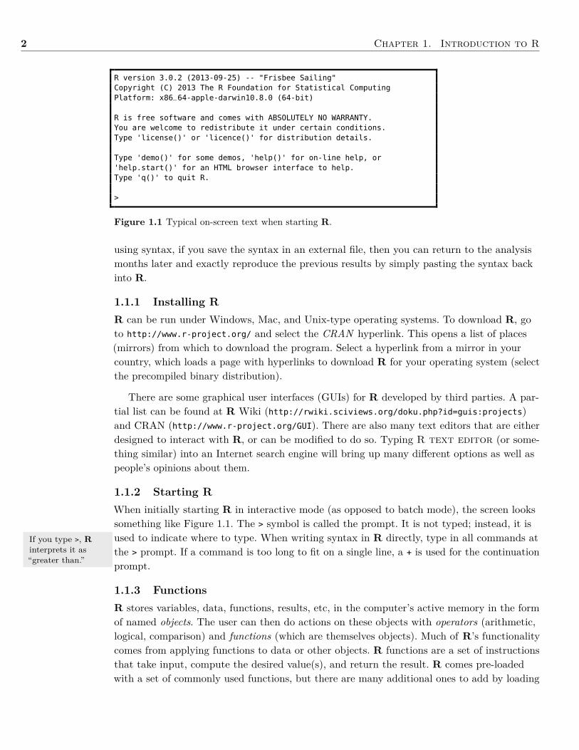
Figure 1.1 Typical on-screen text when starting R.
If you type >, Rinterprets it as“greater than.”
using syntax, if you save the syntax in an external file, then you can return to the analysismonths later and exactly reproduce the previous results by simply pasting the syntax backinto R.
1.1.1 Installing RR can be run under Windows, Mac, and Unix-type operating systems. To download R, goto http://www.r-project.org/ and select the CRAN hyperlink. This opens a list of places(mirrors) from which to download the program. Select a hyperlink from a mirror in yourcountry, which loads a page with hyperlinks to download R for your operating system (selectthe precompiled binary distribution).
There are some graphical user interfaces (GUIs) for R developed by third parties. A par-tial list can be found at R Wiki (http://rwiki.sciviews.org/doku.php?id=guis:projects)and CRAN (http://www.r-project.org/GUI). There are also many text editors that are eitherdesigned to interact with R, or can be modified to do so. Typing R text editor (or some-thing similar) into an Internet search engine will bring up many different options as well aspeople’s opinions about them.
1.1.2 Starting RWhen initially starting R in interactive mode (as opposed to batch mode), the screen lookssomething like Figure 1.1. The > symbol is called the prompt. It is not typed; instead, it isused to indicate where to type. When writing syntax in R directly, type in all commands atthe > prompt. If a command is too long to fit on a single line, a + is used for the continuationprompt.
1.1.3 FunctionsR stores variables, data, functions, results, etc, in the computer’s active memory in the formof named objects. The user can then do actions on these objects with operators (arithmetic,logical, comparison) and functions (which are themselves objects). Much of R’s functionalitycomes from applying functions to data or other objects. R functions are a set of instructionsthat take input, compute the desired value(s), and return the result. R comes pre-loadedwith a set of commonly used functions, but there are many additional ones to add by loading
1.1. Background 3
packages with the desired functions, or by writing a function. To use functions: (a) give thefunction’s name followed by parentheses; (b) in the parentheses, give the necessary values forthe function’s argument(s).
1.1.3.1 Some Useful FunctionsBelow are helpful R functions that I find myself using repeatedly.
• Comment. This is not really a function, but in R anything after the # sign is assumedto be a comment and R ignores it. Comments are extremely helpful, as annotating Rsyntax can save a lot of future time and effort.
• Assign. Another symbol that most R users will encounter frequently is the left arrow,<-, which is R’s standard assignment operator (another option is using =, but it is bet-ter to reserve using = for defining values for arguments). The <- is R’s way of assigningwhatever is on the right of the arrow to the object on the left of the arrow.
• Concatenate. The concatenate function, c(), concatenates the arguments included inthe function. Using c() in conjunction with <- assigns the concatenated objects into anew object. For example, to make a dataset of 5 observations with the values 4, 5 3, 6,9, and name it newData, I would use the following syntax:
newData <- c(4, 5, 3, 6, 9)
• Help. The help() function returns information about a function (or certain specialwords or characters). A shortcut for help() is a question mark, ?. For example, thefollowing two lines of syntax return the same results.
help(mean)?mean
The help() function returns a page that (at a minimum) describes the function, its argu-ments, and gives some examples of how to use it. Some help pages have much more detailthan others. To just execute the example syntax for a function, use the example() function.
example(mean)
#### mean> x <- c(0:10, 50)#### mean> xm <- mean(x)#### mean> c(xm, mean(x, trim = 0.10))## [1] 8.8 5.5
To obtain help on an entire R package, use the package argument in the help() function.
help(package = psych)
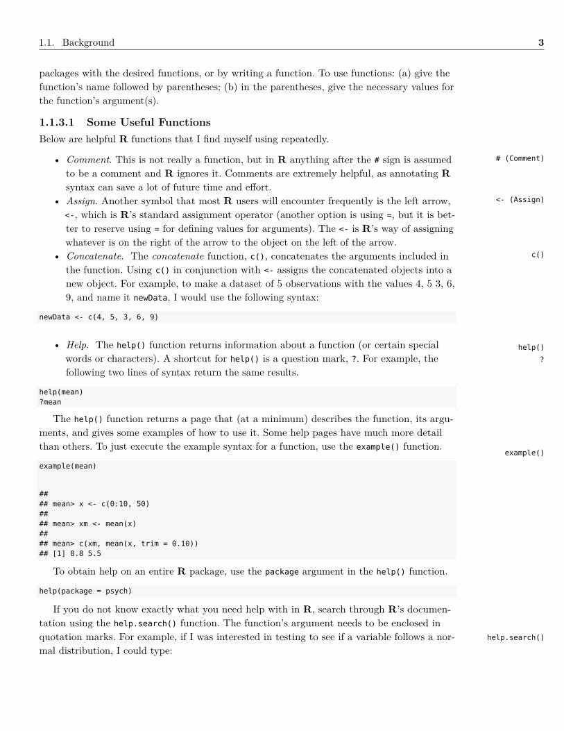
If you do not know exactly what you need help with in R, search through R’s documen-tation using the help.search() function. The function’s argument needs to be enclosed inquotation marks. For example, if I was interested in testing to see if a variable follows a nor-mal distribution, I could type:
# (Comment)
<- (Assign)
c()
help()
?
example()
help.search()
4 Chapter 1. Introduction to R
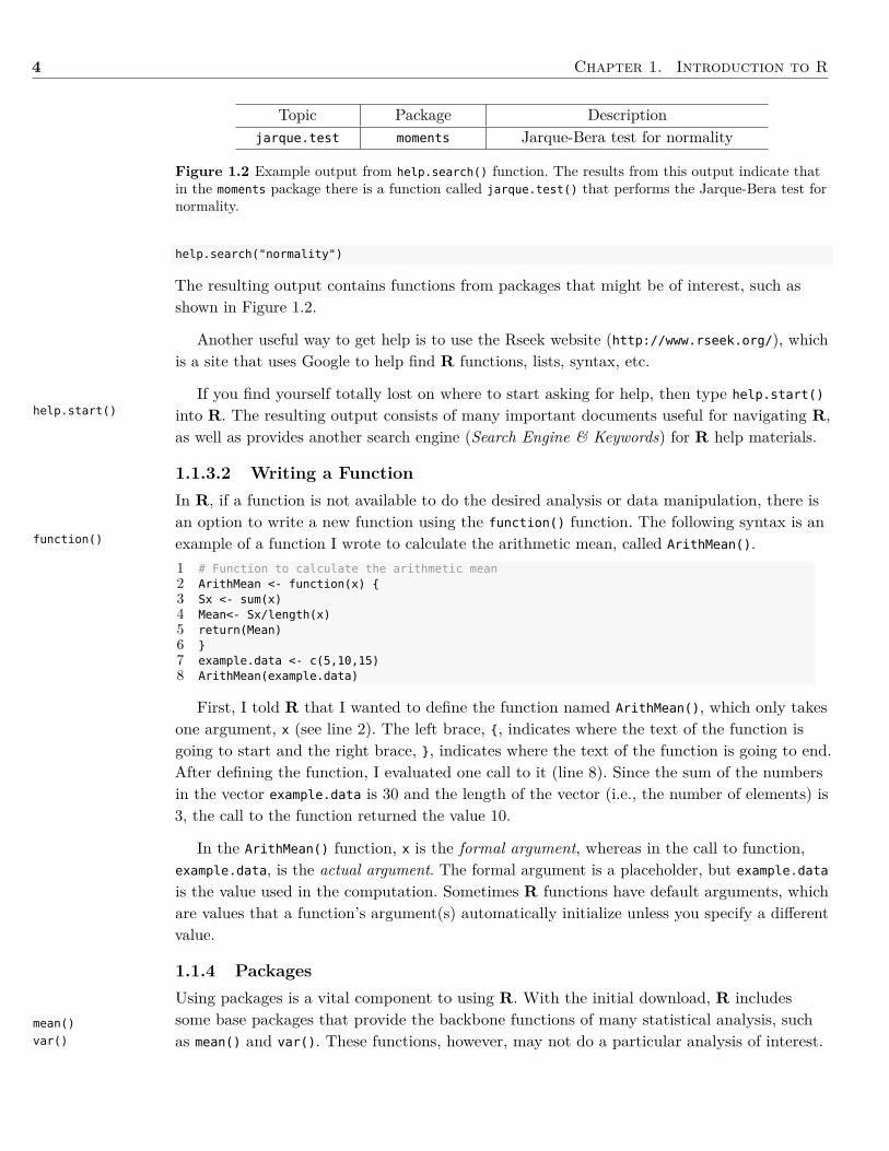
Topic Package Descriptionjarque.test moments Jarque-Bera test for normality
Figure 1.2 Example output from help.search() function. The results from this output indicate thatin the moments package there is a function called jarque.test() that performs the Jarque-Bera test fornormality.
help.start()
function()
mean()
var()
help.search("normality")
The resulting output contains functions from packages that might be of interest, such asshown in Figure 1.2.
Another useful way to get help is to use the Rseek website (http://www.rseek.org/), whichis a site that uses Google to help find R functions, lists, syntax, etc.
If you find yourself totally lost on where to start asking for help, then type help.start()
into R. The resulting output consists of many important documents useful for navigating R,as well as provides another search engine (Search Engine & Keywords) for R help materials.
1.1.3.2 Writing a FunctionIn R, if a function is not available to do the desired analysis or data manipulation, there isan option to write a new function using the function() function. The following syntax is anexample of a function I wrote to calculate the arithmetic mean, called ArithMean().1 # Function to calculate the arithmetic mean2 ArithMean <- function(x) {3 Sx <- sum(x)4 Mean<- Sx/length(x)5 return(Mean)6 }7 example.data <- c(5,10,15)8 ArithMean(example.data)
First, I told R that I wanted to define the function named ArithMean(), which only takesone argument, x (see line 2). The left brace, {, indicates where the text of the function isgoing to start and the right brace, }, indicates where the text of the function is going to end.After defining the function, I evaluated one call to it (line 8). Since the sum of the numbersin the vector example.data is 30 and the length of the vector (i.e., the number of elements) is3, the call to the function returned the value 10.
In the ArithMean() function, x is the formal argument, whereas in the call to function,example.data, is the actual argument. The formal argument is a placeholder, but example.datais the value used in the computation. Sometimes R functions have default arguments, whichare values that a function’s argument(s) automatically initialize unless you specify a differentvalue.
1.1.4 PackagesUsing packages is a vital component to using R. With the initial download, R includessome base packages that provide the backbone functions of many statistical analysis, suchas mean() and var(). These functions, however, may not do a particular analysis of interest.
1.1. Background 5
Thus, I can see if a contributed R package has a function for the needed analysis. These Rpackages usually consist of functions and example data that were written in the R language(although sometimes they are written in FORTRAN or C and then linked back into R).
The ability for users to contribute packages is extremely powerful, as there are manyexperts across a variety of fields who have contributed packages that contain functions tocompute almost any statistical analysis. A list of R packages, along with a short descrip-tion of what they do, can be found in CRAN, but it is very long and hard to navigate un-less looking for a specific package by name. An alternative is to examine CRAN task views[http://cran.r-project.org/web/views/], which is designed to help users find packages asso-ciated with specific types of fields or analyses. For example, the Psychometrics view [http://cran.r-project.org/web/views/Psychometrics.html] has many packages dealing with itemand test analysis.
To install a package, use the (oddly enough named!) install.packages() function, namingthe package to install in quotation marks. For example, to install the BaylorEdPsych pack-age, I use the following syntax:
install.packages("BaylorEdPsych", dep = TRUE)
The dep = TRUE argument tells R that, in addition to the package of interest, I also wantto download any other package upon which the package of interest is dependent. Installingthe dependent packages saves the time of having to download each required package sepa-rately. Packages only need to installed on a computer’s hard disk once, but need to be loadedinto R’s memory each time R is restarted and there is a need to use one of the package’sfunctions. Load an already-installed package by using the library() function.
library(BaylorEdPsych)
Since R is case sensitive, Install.packages("BaylorEdPsych", dep = TRUE),install.packages("BaylorEdpsych", dep = TRUE), install.Packages("BaylorEdPsych",
dep = TRUE), or any other permutation will result in an error message.
1.1.5 Data Input
1.1.5.1 ConcatenateThe easiest way to enter data into R is to directly type it using the c() function, and thenassign it to an object. To verify that the data are in the object (in this case, a vector), justtype the object’s name.
newData <- c(4, 5, 3, 6, 9)newData
## [1] 4 5 3 6 9
Once the data is in an R object, I can then apply functions to the object, e.g.,
install.packages()
The interactiveversion of R pro-vides an alternativemethod of installingpackages via thePackages & Datamenu.
library()
6 Chapter 1. Introduction to R
Variable names needto start with let-ters.
Besides a period,variable namesshould not haveany other non-alphanumeric charac-ters.
You can use otherextensions for datafiles, such as .dat.
read.table()
read.csv()
file.choose()
mean(newData)sum(newData)
1.1.5.2 Import Data from an External SourceUnless the dataset has one variable with a few observations (e.g., data from a textbook exam-ple), it is usually better to store the data in an external file and then import into R. Here arethree suggestions when saving data in an external file.
• Code all missing values to NA, which is the default indicator in R for a missing value.• Make sure the variable names do not have spaces. Use a period in lieu of a space (e.g.,
first.name).• Save the data as a plain text file, using either tabs, spaces, or commas as delimiters.
Typically when data storage programs export space- or tab-delimited files they appenda .txt extension and use a .csv extension for comma-delimited files. Most spreadsheetand database programs can export data in at least one of these formats.
After the data are properly stored in the external file, the read.table() function can im-port the externally stored data. The main argument for this function is the external file’sname and location. R requires the use of a forward slash or double backslash to indicate afile location. For example, say I stored a dataset in a file named data.csv, which I stored ina folder named name that is further nested in a folder named file. To import the data usingany of the following syntaxes.# Windowsnew.data <- read.table("C:\\file\\name\\data.csv", sep = ",")new.data <- read.csv("C:\\file\\name\\data.csv")new.data <- read.csv("C:/file/name/data.csv")
# Mac and Unix-type systemsnew.data <- read.table("/Users/first_last/file/name/data.csv", sep = ",")new.data <- read.csv("/Users/first_last/file/name/data.csv")
The sep argument tell the function how the variables are delimited in the data file. The de-fault option is tab delimitation, so specifying sep="," is needed to indicate comma delimita-tion. The read.csv() function works just like the read.table() function, only it assumes thedata are comma-delimited.
By default, the read.table() function returns a data frame. A data frame is a type of Robject that stores variables as columns. Data frames are useful as they can store differenttypes of variables, such as strings and numbers.
If the location of the data file is under many sublayers of folders, (or, more typically forme, I forget its exact location), I can search for file using the file.choose() function.new.data <- read.table(file.choose(), header = TRUE, sep = ",")
This opens a dialog box that allows me to choose the file interactively.
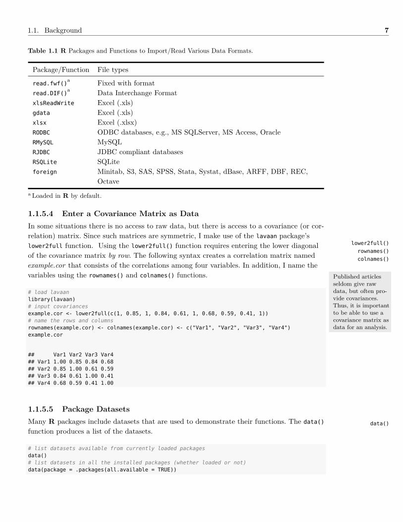
1.1.5.3 Import Other Programs’ DataR can read in data from file formats other than plain text. Table 1.1 lists some packages andfunctions along with the data types they read.
1.1. Background 7
Table 1.1 R Packages and Functions to Import/Read Various Data Formats.
Package/Function File types
read.fwf()a Fixed with format
read.DIF()a Data Interchange Format
xlsReadWrite Excel (.xls)gdata Excel (.xls)xlsx Excel (.xlsx)RODBC ODBC databases, e.g., MS SQLServer, MS Access, OracleRMySQL MySQLRJDBC JDBC compliant databasesRSQLite SQLiteforeign Minitab, S3, SAS, SPSS, Stata, Systat, dBase, ARFF, DBF, REC,
Octavea Loaded in R by default.
1.1.5.4 Enter a Covariance Matrix as DataIn some situations there is no access to raw data, but there is access to a covariance (or cor-relation) matrix. Since such matrices are symmetric, I make use of the lavaan package’slower2full function. Using the lower2full() function requires entering the lower diagonalof the covariance matrix by row. The following syntax creates a correlation matrix namedexample.cor that consists of the correlations among four variables. In addition, I name thevariables using the rownames() and colnames() functions.
# load lavaanlibrary(lavaan)# input covariancesexample.cor <- lower2full(c(1, 0.85, 1, 0.84, 0.61, 1, 0.68, 0.59, 0.41, 1))# name the rows and columnsrownames(example.cor) <- colnames(example.cor) <- c("Var1", "Var2", "Var3", "Var4")example.cor
## Var1 Var2 Var3 Var4## Var1 1.00 0.85 0.84 0.68## Var2 0.85 1.00 0.61 0.59## Var3 0.84 0.61 1.00 0.41## Var4 0.68 0.59 0.41 1.00
1.1.5.5 Package DatasetsMany R packages include datasets that are used to demonstrate their functions. The data()
function produces a list of the datasets.
# list datasets available from currently loaded packagesdata()# list datasets in all the installed packages (whether loaded or not)data(package = .packages(all.available = TRUE))
lower2full()
rownames()
colnames()
Published articlesseldom give rawdata, but often pro-vide covariances.Thus, it is importantto be able to use acovariance matrix asdata for an analysis.
data()
8 Chapter 1. Introduction to R
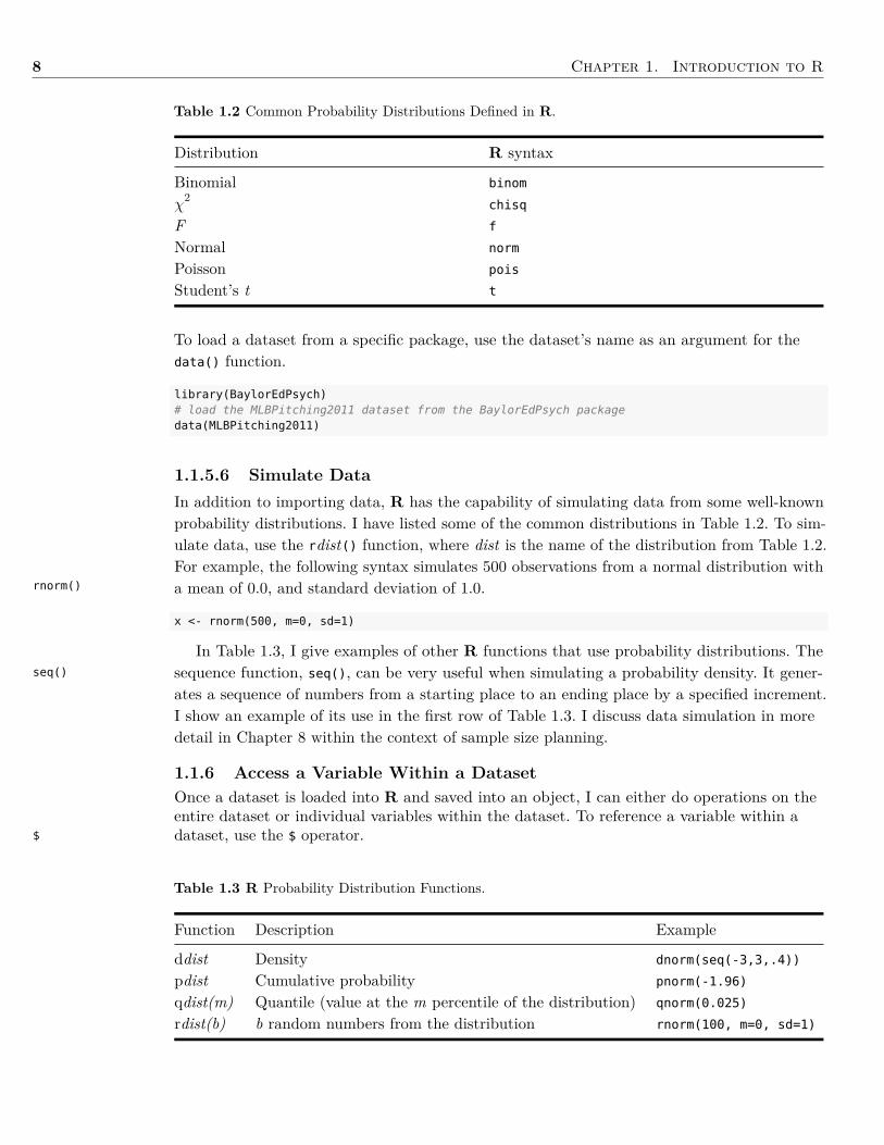
Table 1.2 Common Probability Distributions Defined in R.
Distribution R syntax
Binomial binom
χ2
chisq
F f
Normal norm
Poisson pois
Student’s t t
rnorm()
seq()
$
To load a dataset from a specific package, use the dataset’s name as an argument for thedata() function.
library(BaylorEdPsych)# load the MLBPitching2011 dataset from the BaylorEdPsych packagedata(MLBPitching2011)
1.1.5.6 Simulate DataIn addition to importing data, R has the capability of simulating data from some well-knownprobability distributions. I have listed some of the common distributions in Table 1.2. To sim-ulate data, use the rdist() function, where dist is the name of the distribution from Table 1.2.For example, the following syntax simulates 500 observations from a normal distribution witha mean of 0.0, and standard deviation of 1.0.
x <- rnorm(500, m=0, sd=1)
In Table 1.3, I give examples of other R functions that use probability distributions. Thesequence function, seq(), can be very useful when simulating a probability density. It gener-ates a sequence of numbers from a starting place to an ending place by a specified increment.I show an example of its use in the first row of Table 1.3. I discuss data simulation in moredetail in Chapter 8 within the context of sample size planning.
1.1.6 Access a Variable Within a DatasetOnce a dataset is loaded into R and saved into an object, I can either do operations on theentire dataset or individual variables within the dataset. To reference a variable within adataset, use the $ operator.
Table 1.3 R Probability Distribution Functions.
Function Description Example
ddist Density dnorm(seq(-3,3,.4))
pdist Cumulative probability pnorm(-1.96)
qdist(m) Quantile (value at the m percentile of the distribution) qnorm(0.025)
rdist(b) b random numbers from the distribution rnorm(100, m=0, sd=1)
1.1. Background 9
new.data$variable
An alternative to the $ function is to attach a dataset using the attach() function. Afterattaching a dataset, I can directly access the variables within it.
attach(new.data)variable
Using the attach() function can cause trouble, though, if the name of a dataset’s variableis already being used by R. Specifically, if I attach two datasets to R and both have a vari-able with the same name, R automatically uses the variable from the most recently attacheddataset. An alternative to using attach() is to wrap the syntax in the with() function. Forexample, say I have a dataset named new.data, and a variable in the dataset is named age.The following syntax calculates the mean of the age variable.
with(new.data, mean(age))
Some functions have an argument to specify the dataset to use, in which case there is noneed to use the with() function or $ notation. For example, the following syntax regresses theage variable on the IQ variable in the new.data dataset.1
lm(age ~ IQ, data = new.data)
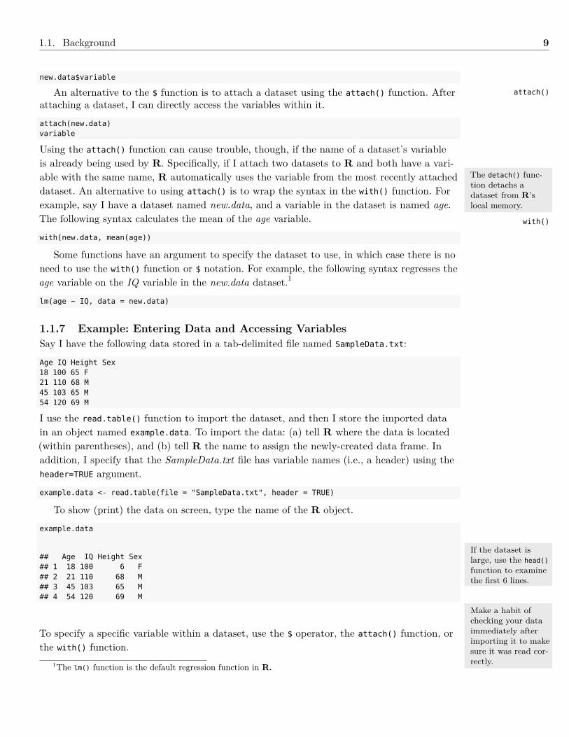
1.1.7 Example: Entering Data and Accessing VariablesSay I have the following data stored in a tab-delimited file named SampleData.txt:
Age IQ Height Sex18 100 65 F21 110 68 M45 103 65 M54 120 69 M
I use the read.table() function to import the dataset, and then I store the imported datain an object named example.data. To import the data: (a) tell R where the data is located(within parentheses), and (b) tell R the name to assign the newly-created data frame. Inaddition, I specify that the SampleData.txt file has variable names (i.e., a header) using theheader=TRUE argument.
example.data <- read.table(file = "SampleData.txt", header = TRUE)
To show (print) the data on screen, type the name of the R object.
example.data
## Age IQ Height Sex## 1 18 100 6 F## 2 21 110 68 M## 3 45 103 65 M## 4 54 120 69 M
To specify a specific variable within a dataset, use the $ operator, the attach() function, orthe with() function.
attach()
The detach() func-tion detachs adataset from R’slocal memory.
with()
If the dataset islarge, use the head()
function to examinethe first 6 lines.
Make a habit ofchecking your dataimmediately afterimporting it to makesure it was read cor-rectly.1The lm() function is the default regression function in R.
10 Chapter 1. Introduction to R
example.data$Age
## [1] 18 21 45 54
with(example.data, Age)
## [1] 18 21 45 54
attach(example.data)Age
## [1] 18 21 45 54
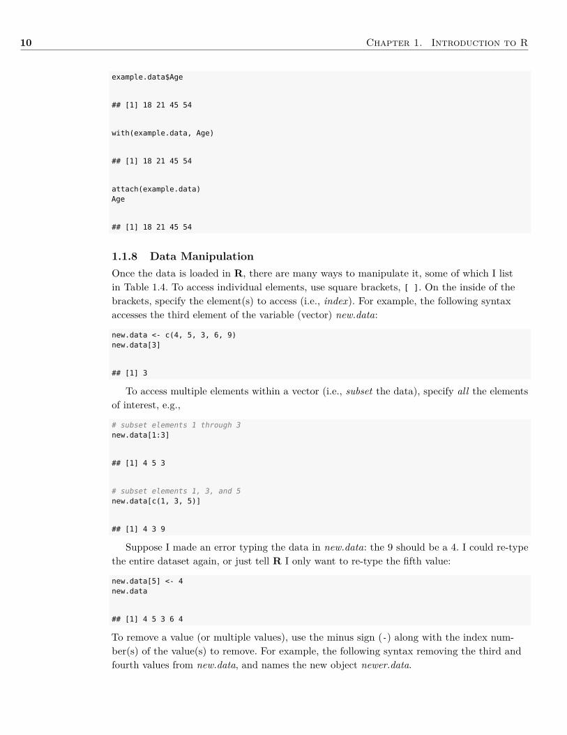
1.1.8 Data ManipulationOnce the data is loaded in R, there are many ways to manipulate it, some of which I listin Table 1.4. To access individual elements, use square brackets, [ ]. On the inside of thebrackets, specify the element(s) to access (i.e., index). For example, the following syntaxaccesses the third element of the variable (vector) new.data:
new.data <- c(4, 5, 3, 6, 9)new.data[3]
## [1] 3
To access multiple elements within a vector (i.e., subset the data), specify all the elementsof interest, e.g.,
# subset elements 1 through 3new.data[1:3]
## [1] 4 5 3
# subset elements 1, 3, and 5new.data[c(1, 3, 5)]
## [1] 4 3 9
Suppose I made an error typing the data in new.data: the 9 should be a 4. I could re-typethe entire dataset again, or just tell R I only want to re-type the fifth value:
new.data[5] <- 4new.data
## [1] 4 5 3 6 4
To remove a value (or multiple values), use the minus sign (-) along with the index num-ber(s) of the value(s) to remove. For example, the following syntax removing the third andfourth values from new.data, and names the new object newer.data.
1.1. Background 11
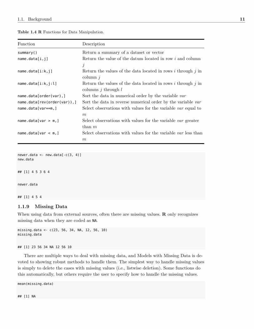
Table 1.4 R Functions for Data Manipulation.
Function Description
summary() Return a summary of a dataset or vectorname.data[i,j] Return the value of the datum located in row i and column
j
name.data[i:k,j] Return the values of the data located in rows i through j incolumn j
name.data[i:k,j:l] Return the values of the data located in rows i through j incolumns j through l
name.data[order(var),] Sort the data in numerical order by the variable varname.data[rev(order(var)),] Sort the data in reverse numerical order by the variable varname.data[var==m,] Select observations with values for the variable var equal to
m
name.data[var > m,] Select observations with values for the variable var greaterthan m
name.data[var < m,] Select observations with values for the variable var less thanm
newer.data <- new.data[-c(3, 4)]new.data
## [1] 4 5 3 6 4
newer.data
## [1] 4 5 4
1.1.9 Missing DataWhen using data from external sources, often there are missing values. R only recognizesmissing data when they are coded as NA.
missing.data <- c(23, 56, 34, NA, 12, 56, 10)missing.data
## [1] 23 56 34 NA 12 56 10
There are multiple ways to deal with missing data, and Models with Missing Data is de-voted to showing robust methods to handle them. The simplest way to handle missing valuesis simply to delete the cases with missing values (i.e., listwise deletion). Some functions dothis automatically, but others require the user to specify how to handle the missing values.
mean(missing.data)
## [1] NA

12 Chapter 1. Introduction to R
na.omit()
These are factorsin the experimentaldesign sense, not thelatent variable sense.
factor()
summary()
describe()
mean(missing.data, na.rm = TRUE)
## [1] 32
Another option is to make a new dataset that removes the missing values using the na.omit()
function.
nomissing.data <- na.omit(missing.data)mean(nomissing.data)
## [1] 32
1.1.10 Categorical DataCategorical variables have a countably finite number of possible values. For such variables,their values can be coded either qualitatively (e.g., “Male”, “Female”) or numerically (e.g.,Male=0, Female=1). If a variable is coded qualitatively, then R has a special data class forthem: factors.
qual.data <- c("Male", "Female", "Female", "Male", "Male")qual.data
## [1] "Male" "Female" "Female" "Male" "Male"
factor(qual.data)
## [1] Male Female Female Male Male## Levels: Female Male
If a categorical variable is coded numerically, R assumes it is a continuous variable unlesstold differently. To make R recognize it as a categorical variable, either make it a factor byusing the factor() function, or qualitatively re-code it.
quant.data <- c(0, 1, 1, 0, 0)# make quant.data a factorquant.data <- factor(quant.data)# make the quant.data qualitative by giving labels to the factorsquant.data <- factor(x = quant.data, levels = 0:1, labels = c("Male", "Female"))quant.data
## [1] Male Female Female Male Male## Levels: Male Female
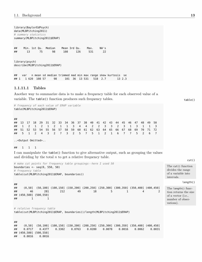
1.1.11 Summarize DataR’s summary() function is the default method of summarizing data. I typically use the psych
package’s describe() function, though, as it provides most of the common summary statis-tics for data description and inspection.
1.1. Background 13
library(BaylorEdPsych)data(MLBPitching2011)# summary statisticssummary(MLBPitching2011$ERAP)
## Min. 1st Qu. Median Mean 3rd Qu. Max. NA's## 13 75 98 108 126 531 22
library(psych)describe(MLBPitching2011$ERAP)
## var n mean sd median trimmed mad min max range skew kurtosis se## 1 1 620 108 57 98 101 36 13 531 518 2.7 13 2.3
1.1.11.1 TablesAnother way to summarize data is to make a frequency table for each observed value of avariable. The table() function produces such frequency tables.
# frequency of each value of ERAP variabletable(MLBPitching2011$ERAP)
#### 13 17 18 29 31 32 33 34 36 37 38 40 41 42 43 44 45 46 47 48 49 50## 1 2 1 2 1 2 1 1 3 4 4 2 2 3 3 2 3 1 3 1 1 3## 51 52 53 54 55 56 57 58 59 60 61 62 63 64 65 66 67 68 69 70 71 72## 5 1 2 4 3 2 7 3 2 5 7 5 1 2 1 6 7 7 5 2 6 7
..<Output Omitted>..
## 1 1 1
I can manipulate the table() function to give alternative output, such as grouping the valuesand dividing by the total n to get a relative frequency table.
# make cut points for frequency table groupings--here I used 50boundaries <- seq(0, 550, 50)# frequency tabletable(cut(MLBPitching2011$ERAP, boundaries))
#### (0,50] (50,100] (100,150] (150,200] (200,250] (250,300] (300,350] (350,400] (400,450]## 46 281 212 49 18 5 1 4 2## (450,500] (500,550]## 1 1
# relative frequency tabletable(cut(MLBPitching2011$ERAP, boundaries))/length(MLBPitching2011$ERAP)
#### (0,50] (50,100] (100,150] (150,200] (200,250] (250,300] (300,350] (350,400] (400,450]## 0.0717 0.4377 0.3302 0.0763 0.0280 0.0078 0.0016 0.0062 0.0031## (450,500] (500,550]## 0.0016 0.0016
table()
cut()
The cut() functiondivides the rangeof a variable intointervals.
length()
The length() func-tion returns the sizeof a vector (i.e.,number of obser-vations).
14 Chapter 1. Introduction to R
cor()
cov()
1.1.12 Common Statistics
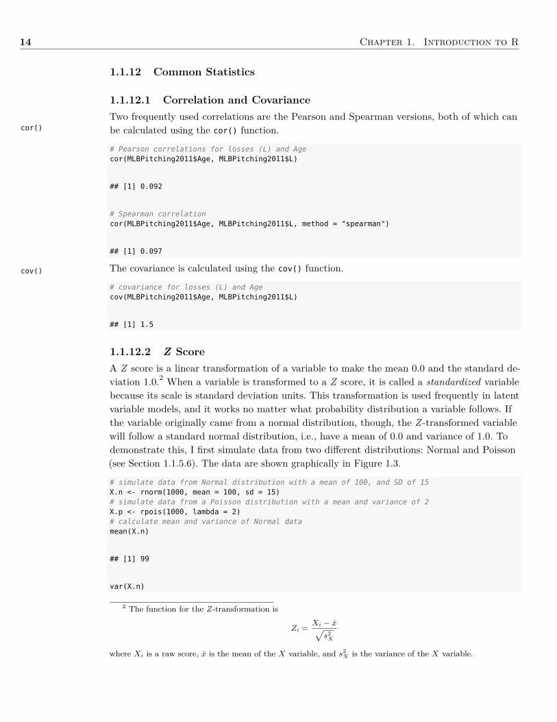
1.1.12.1 Correlation and CovarianceTwo frequently used correlations are the Pearson and Spearman versions, both of which canbe calculated using the cor() function.
# Pearson correlations for losses (L) and Agecor(MLBPitching2011$Age, MLBPitching2011$L)
## [1] 0.092
# Spearman correlationcor(MLBPitching2011$Age, MLBPitching2011$L, method = "spearman")
## [1] 0.097
The covariance is calculated using the cov() function.
# covariance for losses (L) and Agecov(MLBPitching2011$Age, MLBPitching2011$L)
## [1] 1.5
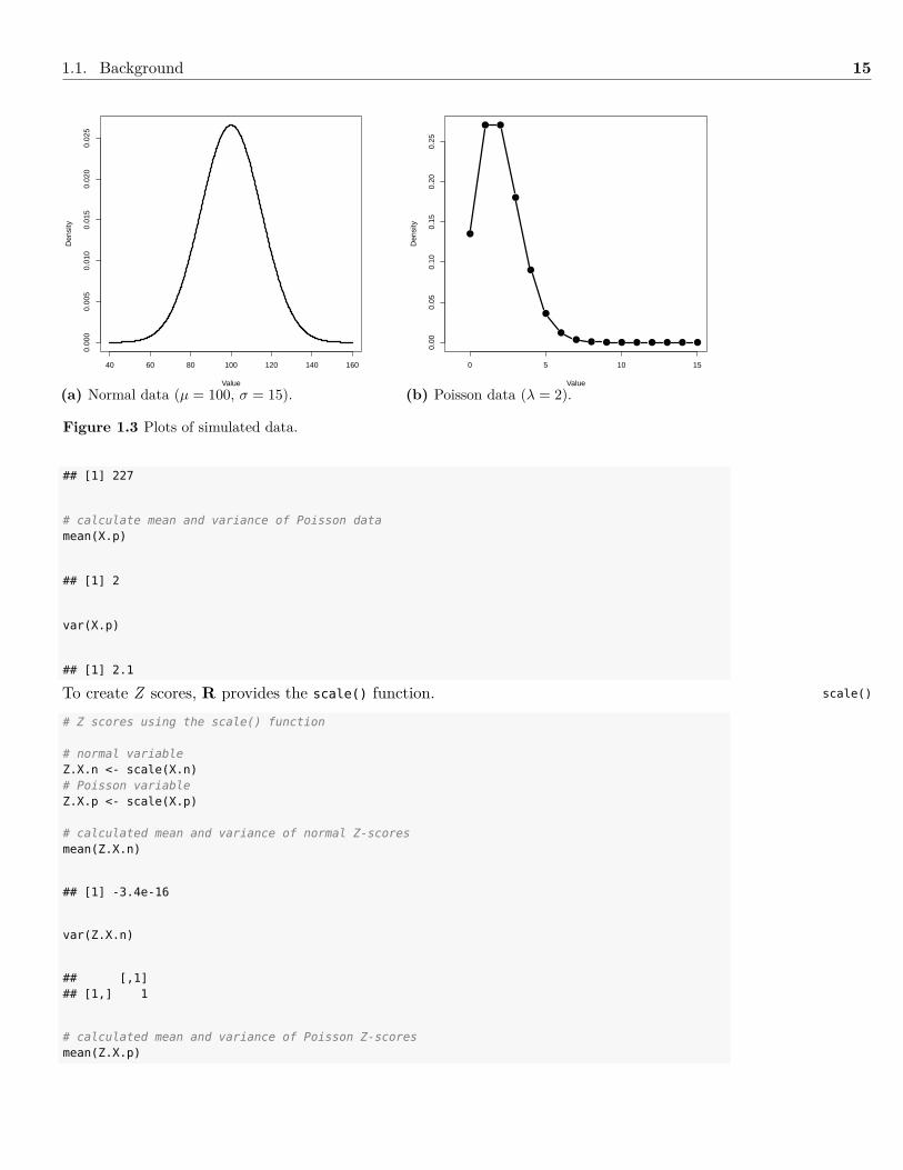
1.1.12.2 Z ScoreA Z score is a linear transformation of a variable to make the mean 0.0 and the standard de-viation 1.0.2 When a variable is transformed to a Z score, it is called a standardized variablebecause its scale is standard deviation units. This transformation is used frequently in latentvariable models, and it works no matter what probability distribution a variable follows. Ifthe variable originally came from a normal distribution, though, the Z -transformed variablewill follow a standard normal distribution, i.e., have a mean of 0.0 and variance of 1.0. Todemonstrate this, I first simulate data from two different distributions: Normal and Poisson(see Section 1.1.5.6). The data are shown graphically in Figure 1.3.
# simulate data from Normal distribution with a mean of 100, and SD of 15X.n <- rnorm(1000, mean = 100, sd = 15)# simulate data from a Poisson distribution with a mean and variance of 2X.p <- rpois(1000, lambda = 2)# calculate mean and variance of Normal datamean(X.n)
## [1] 99
var(X.n)
2 The function for the Z -transformation is
Zi = Xi − x̄√s2
X
where Xi is a raw score, x̄ is the mean of the X variable, and s2X is the variance of the X variable.
1.1. Background 15
40 60 80 100 120 140 160
0.00
00.
005
0.01
00.
015
0.02
00.
025
Value
Den
sity
(a) Normal data (µ = 100, σ = 15).
●
● ●
●
●
●
●
● ● ● ● ● ● ● ● ●
0 5 10 15
0.00
0.05
0.10
0.15
0.20
0.25
Value
Den
sity
(b) Poisson data (λ = 2).
Figure 1.3 Plots of simulated data.
## [1] 227
# calculate mean and variance of Poisson datamean(X.p)
## [1] 2
var(X.p)
## [1] 2.1
To create Z scores, R provides the scale() function.# Z scores using the scale() function
# normal variableZ.X.n <- scale(X.n)# Poisson variableZ.X.p <- scale(X.p)
# calculated mean and variance of normal Z-scoresmean(Z.X.n)
## [1] -3.4e-16
var(Z.X.n)
## [,1]## [1,] 1
# calculated mean and variance of Poisson Z-scoresmean(Z.X.p)
scale()
16 Chapter 1. Introduction to R
z.test()
na.omit()
t.test()
## [1] -6.1e-17
var(Z.X.p)
## [,1]## [1,] 1
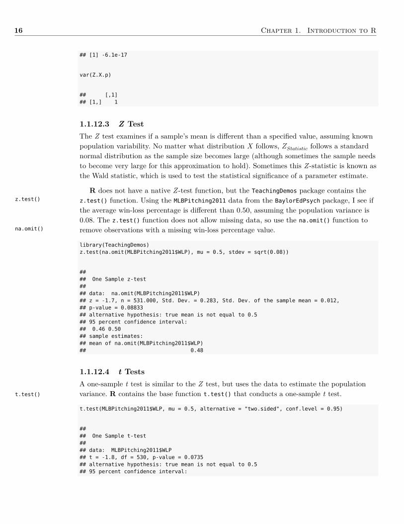
1.1.12.3 Z TestThe Z test examines if a sample’s mean is different than a specified value, assuming knownpopulation variability. No matter what distribution X follows, ZStatistic follows a standardnormal distribution as the sample size becomes large (although sometimes the sample needsto become very large for this approximation to hold). Sometimes this Z -statistic is known asthe Wald statistic, which is used to test the statistical significance of a parameter estimate.
R does not have a native Z -test function, but the TeachingDemos package contains thez.test() function. Using the MLBPitching2011 data from the BaylorEdPsych package, I see ifthe average win-loss percentage is different than 0.50, assuming the population variance is0.08. The z.test() function does not allow missing data, so use the na.omit() function toremove observations with a missing win-loss percentage value.
library(TeachingDemos)z.test(na.omit(MLBPitching2011$WLP), mu = 0.5, stdev = sqrt(0.08))
#### One Sample z-test#### data: na.omit(MLBPitching2011$WLP)## z = -1.7, n = 531.000, Std. Dev. = 0.283, Std. Dev. of the sample mean = 0.012,## p-value = 0.08833## alternative hypothesis: true mean is not equal to 0.5## 95 percent confidence interval:## 0.46 0.50## sample estimates:## mean of na.omit(MLBPitching2011$WLP)## 0.48
1.1.12.4 t TestsA one-sample t test is similar to the Z test, but uses the data to estimate the populationvariance. R contains the base function t.test() that conducts a one-sample t test.
t.test(MLBPitching2011$WLP, mu = 0.5, alternative = "two.sided", conf.level = 0.95)
#### One Sample t-test#### data: MLBPitching2011$WLP## t = -1.8, df = 530, p-value = 0.0735## alternative hypothesis: true mean is not equal to 0.5## 95 percent confidence interval:
1.1. Background 17
## 0.46 0.50## sample estimates:## mean of x## 0.48
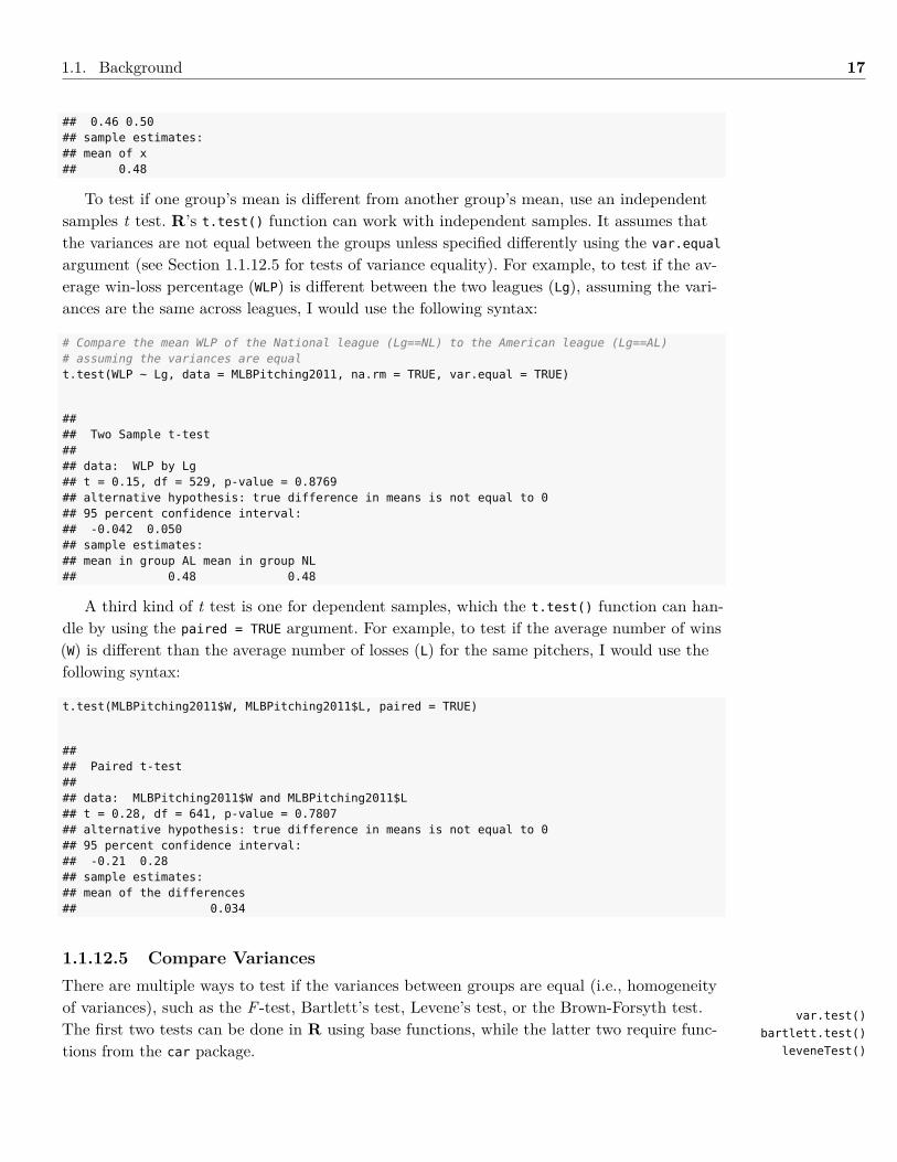
To test if one group’s mean is different from another group’s mean, use an independentsamples t test. R’s t.test() function can work with independent samples. It assumes thatthe variances are not equal between the groups unless specified differently using the var.equal
argument (see Section 1.1.12.5 for tests of variance equality). For example, to test if the av-erage win-loss percentage (WLP) is different between the two leagues (Lg), assuming the vari-ances are the same across leagues, I would use the following syntax:
# Compare the mean WLP of the National league (Lg==NL) to the American league (Lg==AL)# assuming the variances are equalt.test(WLP ~ Lg, data = MLBPitching2011, na.rm = TRUE, var.equal = TRUE)
#### Two Sample t-test#### data: WLP by Lg## t = 0.15, df = 529, p-value = 0.8769## alternative hypothesis: true difference in means is not equal to 0## 95 percent confidence interval:## -0.042 0.050## sample estimates:## mean in group AL mean in group NL## 0.48 0.48
A third kind of t test is one for dependent samples, which the t.test() function can han-dle by using the paired = TRUE argument. For example, to test if the average number of wins(W) is different than the average number of losses (L) for the same pitchers, I would use thefollowing syntax:
t.test(MLBPitching2011$W, MLBPitching2011$L, paired = TRUE)
#### Paired t-test#### data: MLBPitching2011$W and MLBPitching2011$L## t = 0.28, df = 641, p-value = 0.7807## alternative hypothesis: true difference in means is not equal to 0## 95 percent confidence interval:## -0.21 0.28## sample estimates:## mean of the differences## 0.034
1.1.12.5 Compare VariancesThere are multiple ways to test if the variances between groups are equal (i.e., homogeneityof variances), such as the F -test, Bartlett’s test, Levene’s test, or the Brown-Forsyth test.The first two tests can be done in R using base functions, while the latter two require func-tions from the car package.
var.test()
bartlett.test()
leveneTest()
18 Chapter 1. Introduction to R
source()
There are many texteditors for R. Mostof them allow you totry the product forfree, so I suggest try-ing many differenteditors to see whichone best fits yourneeds.
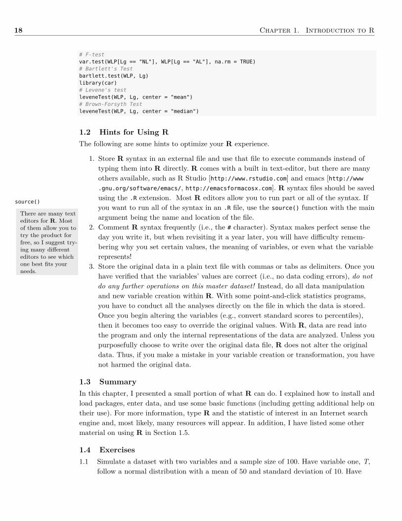
# F-testvar.test(WLP[Lg == "NL"], WLP[Lg == "AL"], na.rm = TRUE)# Bartlett's Testbartlett.test(WLP, Lg)library(car)# Levene's testleveneTest(WLP, Lg, center = "mean")# Brown-Forsyth TestleveneTest(WLP, Lg, center = "median")
1.2 Hints for Using RThe following are some hints to optimize your R experience.
1. Store R syntax in an external file and use that file to execute commands instead oftyping them into R directly. R comes with a built in text-editor, but there are manyothers available, such as R Studio [http://www.rstudio.com] and emacs [http://www.gnu.org/software/emacs/, http://emacsformacosx.com]. R syntax files should be savedusing the .R extension. Most R editors allow you to run part or all of the syntax. Ifyou want to run all of the syntax in an .R file, use the source() function with the mainargument being the name and location of the file.
2. Comment R syntax frequently (i.e., the # character). Syntax makes perfect sense theday you write it, but when revisiting it a year later, you will have difficulty remem-bering why you set certain values, the meaning of variables, or even what the variablerepresents!
3. Store the original data in a plain text file with commas or tabs as delimiters. Once youhave verified that the variables’ values are correct (i.e., no data coding errors), do notdo any further operations on this master dataset! Instead, do all data manipulationand new variable creation within R. With some point-and-click statistics programs,you have to conduct all the analyses directly on the file in which the data is stored.Once you begin altering the variables (e.g., convert standard scores to percentiles),then it becomes too easy to override the original values. With R, data are read intothe program and only the internal representations of the data are analyzed. Unless youpurposefully choose to write over the original data file, R does not alter the originaldata. Thus, if you make a mistake in your variable creation or transformation, you havenot harmed the original data.
1.3 SummaryIn this chapter, I presented a small portion of what R can do. I explained how to install andload packages, enter data, and use some basic functions (including getting additional help ontheir use). For more information, type R and the statistic of interest in an Internet searchengine and, most likely, many resources will appear. In addition, I have listed some othermaterial on using R in Section 1.5.
1.4 Exercises1.1 Simulate a dataset with two variables and a sample size of 100. Have variable one, T,
follow a normal distribution with a mean of 50 and standard deviation of 10. Have
1.4. Exercises 19
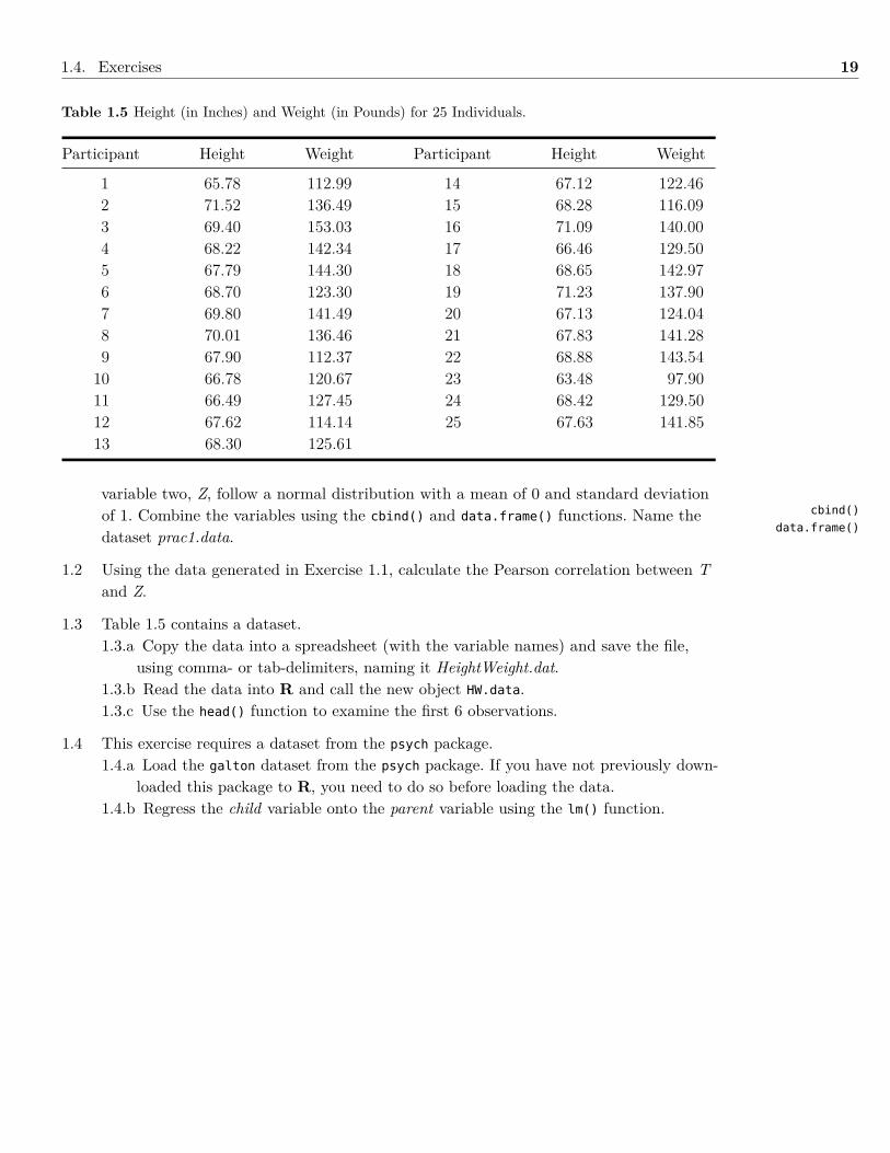
Table 1.5 Height (in Inches) and Weight (in Pounds) for 25 Individuals.
Participant Height Weight Participant Height Weight
1 65.78 112.99 14 67.12 122.462 71.52 136.49 15 68.28 116.093 69.40 153.03 16 71.09 140.004 68.22 142.34 17 66.46 129.505 67.79 144.30 18 68.65 142.976 68.70 123.30 19 71.23 137.907 69.80 141.49 20 67.13 124.048 70.01 136.46 21 67.83 141.289 67.90 112.37 22 68.88 143.54
10 66.78 120.67 23 63.48 97.9011 66.49 127.45 24 68.42 129.5012 67.62 114.14 25 67.63 141.8513 68.30 125.61
variable two, Z, follow a normal distribution with a mean of 0 and standard deviationof 1. Combine the variables using the cbind() and data.frame() functions. Name thedataset prac1.data.
1.2 Using the data generated in Exercise 1.1, calculate the Pearson correlation between Tand Z.
1.3 Table 1.5 contains a dataset.1.3.a Copy the data into a spreadsheet (with the variable names) and save the file,
using comma- or tab-delimiters, naming it HeightWeight.dat.1.3.b Read the data into R and call the new object HW.data.1.3.c Use the head() function to examine the first 6 observations.
1.4 This exercise requires a dataset from the psych package.1.4.a Load the galton dataset from the psych package. If you have not previously down-
loaded this package to R, you need to do so before loading the data.1.4.b Regress the child variable onto the parent variable using the lm() function.
cbind()
data.frame()
20 Chapter 1. Introduction to R
1.5 References & Further ReadingsBeaujean, A. A. (2012). BaylorEdPsych: R package for Baylor University Educational
Psychology quantitative courses (Version 0.5) [Computer software]. Waco, TX: BaylorUniversity.
R Development Core Team. (2013). R: A language and environment for statistical computing[Computer program]. Vienna, Austria: R Foundation for Statistical Computing.
Crawley, M. J. (2013). The R book (2nd ed.). Hoboken, NJ: Wiley.Field, A., Miles, J., & Field, Z. (2012). Discovering statistics using R. Thousand Oaks, CA:
Sage.Matloff, N. (2011). The art of R programming: A tour of statistical software design. San
Francisco, CA: No Starch Press.Revelle, W. (2012). psych: Procedures for psychological, psychometric, and personality research
[Computer program]. Evanston, IL: Northwestern University.
2 | Path Models and Analysis
Chapter Contents2.1 Background . . . . . . . . . . . . . . . . . . . . . . . . . . . . . . . . . . . . 21
2.1.1 Variables Relationships in a Path Model . . . . . . . . . . . . . . . . 212.1.2 Path Model Variations . . . . . . . . . . . . . . . . . . . . . . . . . . 232.1.3 Tracing Rules . . . . . . . . . . . . . . . . . . . . . . . . . . . . . . . 232.1.4 Obtaining a Numerical Solution . . . . . . . . . . . . . . . . . . . . . 242.1.5 Path Coefficients . . . . . . . . . . . . . . . . . . . . . . . . . . . . . 26
2.2 Using R For Path Analysis . . . . . . . . . . . . . . . . . . . . . . . . . . . . 272.2.1 The lavaan Package . . . . . . . . . . . . . . . . . . . . . . . . . . . 27
2.3 Example: Path Analysis using lavaan . . . . . . . . . . . . . . . . . . . . . . 292.4 Indirect Effect . . . . . . . . . . . . . . . . . . . . . . . . . . . . . . . . . . . 30
2.4.1 Example: Indirect Effects . . . . . . . . . . . . . . . . . . . . . . . . 312.5 Summary . . . . . . . . . . . . . . . . . . . . . . . . . . . . . . . . . . . . . . 322.6 Writing the Results . . . . . . . . . . . . . . . . . . . . . . . . . . . . . . . . 322.7 Exercises . . . . . . . . . . . . . . . . . . . . . . . . . . . . . . . . . . . . . . 342.8 References & Further Readings . . . . . . . . . . . . . . . . . . . . . . . . . . 36
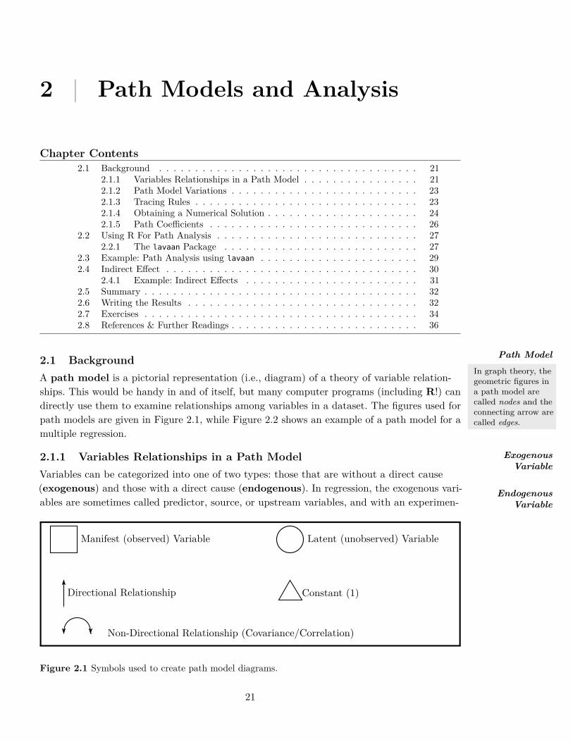
2.1 BackgroundA path model is a pictorial representation (i.e., diagram) of a theory of variable relation-ships. This would be handy in and of itself, but many computer programs (including R!) candirectly use them to examine relationships among variables in a dataset. The figures used forpath models are given in Figure 2.1, while Figure 2.2 shows an example of a path model for amultiple regression.
2.1.1 Variables Relationships in a Path ModelVariables can be categorized into one of two types: those that are without a direct cause(exogenous) and those with a direct cause (endogenous). In regression, the exogenous vari-ables are sometimes called predictor, source, or upstream variables, and with an experimen-
Path ModelIn graph theory, thegeometric figures ina path model arecalled nodes and theconnecting arrow arecalled edges.
ExogenousVariable
EndogenousVariable
Manifest (observed) Variable Latent (unobserved) Variable
Constant (1)Directional Relationship
Non-Directional Relationship (Covariance/Correlation)
Figure 2.1 Symbols used to create path model diagrams.
21
22 Chapter 2. Path Models and Analysis
X2X1 X3
Y
Error
z
a b c
1
d f
e
(a) Standardized model:Y = aX1 + bX2 + cX3 + Error.
X2X1 X3
Y1
Error
z
a b c
1
g
d f
e
(b) Unstandardized model:Y = aX1 + bX2 + cX3 + g + Error.
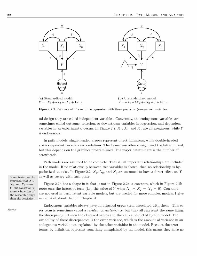
Figure 2.2 Path model of a multiple regression with three predictor (exogenous) variables.
Some texts use thelanguage that X1,X2, and X3 causeY, but causation ismore a function ofthe research designthan the statistics.
Error
tal design they are called independent variables. Conversely, the endogenous variables aresometimes called outcome, criterion, or downstream variables in regression, and dependentvariables in an experimental design. In Figure 2.2, X1, X2, and X3 are all exogenous, while Yis endogenous.
In path models, single-headed arrows represent direct influences, while double-headedarrows represent covariance/correlations. The former are often straight and the latter curved,but this depends on the graphics program used. The major determinant is the number ofarrowheads.
Path models are assumed to be complete. That is, all important relationships are includedin the model. If no relationship between two variables is shown, then no relationship is hy-pothesized to exist. In Figure 2.2, X1, X2, and X3 are assumed to have a direct effect on Yas well as covary with each other.
Figure 2.2b has a shape in it that is not in Figure 2.2a: a constant, which in Figure 2.2brepresents the intercept term (i.e., the value of Y when X1 = X2 = X3 = 0). Constantsare not used in basic latent variable models, but are needed for more complex models. I givemore detail about them in Chapter 4.
Endogenous variables always have an attached error term associated with them. This er-ror term is sometimes called a residual or disturbance, but they all represent the same thing:the discrepancy between the observed values and the values predicted by the model. Thevariability of these discrepancies is the error variance, which is the amount of variance in anendogenous variable not explained by the other variables in the model. Because the errorterms, by definition, represent something unexplained by the model, this means they have no
2.1. Background 23
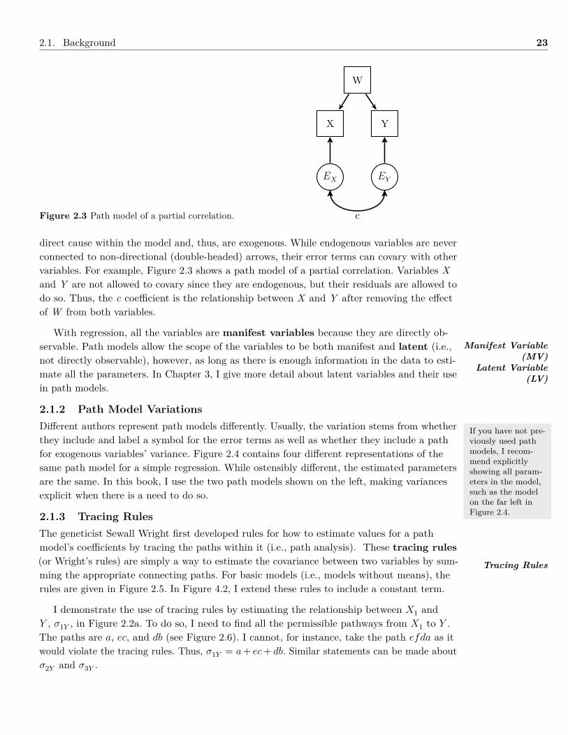
Figure 2.3 Path model of a partial correlation.
W
X Y
EX EY
c
direct cause within the model and, thus, are exogenous. While endogenous variables are neverconnected to non-directional (double-headed) arrows, their error terms can covary with othervariables. For example, Figure 2.3 shows a path model of a partial correlation. Variables Xand Y are not allowed to covary since they are endogenous, but their residuals are allowed todo so. Thus, the c coefficient is the relationship between X and Y after removing the effectof W from both variables.
With regression, all the variables are manifest variables because they are directly ob-servable. Path models allow the scope of the variables to be both manifest and latent (i.e.,not directly observable), however, as long as there is enough information in the data to esti-mate all the parameters. In Chapter 3, I give more detail about latent variables and their usein path models.
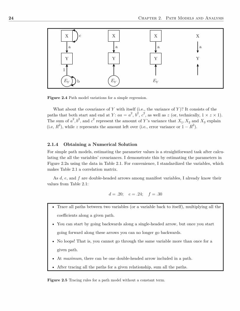
2.1.2 Path Model VariationsDifferent authors represent path models differently. Usually, the variation stems from whetherthey include and label a symbol for the error terms as well as whether they include a pathfor exogenous variables’ variance. Figure 2.4 contains four different representations of thesame path model for a simple regression. While ostensibly different, the estimated parametersare the same. In this book, I use the two path models shown on the left, making variancesexplicit when there is a need to do so.
2.1.3 Tracing RulesThe geneticist Sewall Wright first developed rules for how to estimate values for a pathmodel’s coefficients by tracing the paths within it (i.e., path analysis). These tracing rules(or Wright’s rules) are simply a way to estimate the covariance between two variables by sum-ming the appropriate connecting paths. For basic models (i.e., models without means), therules are given in Figure 2.5. In Figure 4.2, I extend these rules to include a constant term.
I demonstrate the use of tracing rules by estimating the relationship between X1 andY , σ1Y , in Figure 2.2a. To do so, I need to find all the permissible pathways from X1 to Y .The paths are a, ec, and db (see Figure 2.6). I cannot, for instance, take the path efda as itwould violate the tracing rules. Thus, σ1Y = a+ ec+ db. Similar statements can be made aboutσ2Y and σ3Y .
Manifest Variable(MV)
Latent Variable(LV)
If you have not pre-viously used pathmodels, I recom-mend explicitlyshowing all param-eters in the model,such as the modelon the far left inFigure 2.4.
Tracing Rules
24 Chapter 2. Path Models and Analysis
X
Y
EY
a
1
b
c X
Y
EY
a
X
Y
EY
a
X
Y
a
Figure 2.4 Path model variations for a simple regression.
What about the covariance of Y with itself (i.e., the variance of Y )? It consists of thepaths that both start and end at Y : aa = a
2, b2, c2, as well as z (or, technically, 1 × z × 1).The sum of a2
, b2, and c2 represent the amount of Y ’s variance that X1, X2 and X3 explain
(i.e, R2), while z represents the amount left over (i.e., error variance or 1−R2).
2.1.4 Obtaining a Numerical SolutionFor simple path models, estimating the parameter values is a straightforward task after calcu-lating the all the variables’ covariances. I demonstrate this by estimating the parameters inFigure 2.2a using the data in Table 2.1. For convenience, I standardized the variables, whichmakes Table 2.1 a correlation matrix.
As d, e, and f are double-headed arrows among manifest variables, I already know theirvalues from Table 2.1:
d = .20; e = .24; f = .30
• Trace all paths between two variables (or a variable back to itself), multiplying all the
coefficients along a given path.
• You can start by going backwards along a single-headed arrow, but once you start
going forward along these arrows you can no longer go backwards.
• No loops! That is, you cannot go through the same variable more than once for a
given path.
• At maximum, there can be one double-headed arrow included in a path.
• After tracing all the paths for a given relationship, sum all the paths.
Figure 2.5 Tracing rules for a path model without a constant term.
2.1. Background 25
X2X1 X3
Y
Error
a b c
d
e
f
1
z
X2X1 X3
Y
Error
a b c
d f
e
1
z
X2X1 X3
Y
Error
a b c
e
fd
1
z
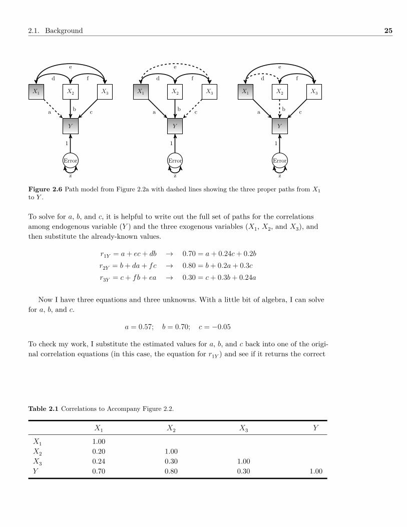
Figure 2.6 Path model from Figure 2.2a with dashed lines showing the three proper paths from X1to Y .
To solve for a, b, and c, it is helpful to write out the full set of paths for the correlationsamong endogenous variable (Y ) and the three exogenous variables (X1, X2, and X3), andthen substitute the already-known values.
r1Y = a+ ec+ db → 0.70 = a+ 0.24c+ 0.2br2Y = b+ da+ fc → 0.80 = b+ 0.2a+ 0.3cr3Y = c+ fb+ ea → 0.30 = c+ 0.3b+ 0.24a
Now I have three equations and three unknowns. With a little bit of algebra, I can solvefor a, b, and c.
a = 0.57; b = 0.70; c = −0.05
To check my work, I substitute the estimated values for a, b, and c back into one of the origi-nal correlation equations (in this case, the equation for r1Y ) and see if it returns the correct
Table 2.1 Correlations to Accompany Figure 2.2.
X1 X2 X3 Y
X1 1.00X2 0.20 1.00X3 0.24 0.30 1.00Y 0.70 0.80 0.30 1.00
26 Chapter 2. Path Models and Analysis
Path Coefficient
value.
r1Y = 0.70 = a+ 0.24c+ 0.20b0.70 = 0.57 + 0.24(−0.05) + 0.20(0.70)0.70 = 0.57− 0.01 + 0.140.70 = 0.70
To solve for z, I follow the same steps as solving for a, b, and c, noting that rY Y = σ2Y Y =
1 since the variables are standardized.
rY Y = a2 + b2 + c2 + 2(cea) + 2(cfb) + 2(bda) + z
1.00 = 0.572 + 0.702 +−0.052 + 2(−0.05)(0.24)(0.57)+2(−0.05)(0.30)(0.70) + 2(0.70)(0.20)(0.57) + z
1.00 = 0.335 + 0.490 + 0.002 +−0.014 +−0.021 + 0.160 + z
1.00− 0.942 = z
0.058 = z
To estimate the amount of Y ’s variance the predictor variables explain (i.e., R2), I use thesame formula I used for rY Y , but leave out the error term (z).
R2 = a2 + b2 + c2 + 2(cea) + 2(cfb) + 2(bda) = 0.942
2.1.5 Path CoefficientsThe values of d − f in Figure 2.6 are correlation coefficients, but what are the values a, b,and c? They are standardized partial regression coefficients, often referred to as just pathcoefficients. Standardized means are variables transformed to Z scores, which places themon standard deviation units (see Section 1.1.12.2); partial regression means that it is therelationship between an exogenous and endogenous variable, controlling for all the otherexogenous variables going to that endogenous variable.
It is not required that the path coefficients be standardized. The variables could just aseasily have been in their natural metric (i.e., raw score units), which would have made thepath coefficients unstandardized.The situation is the same as in multiple regression when deal-ing with standardized (b∗) versus unstandardized (b) coefficients, and the tradeoffs mentionedthere for both types of coefficients apply here as well.1 Usually standardized values are betterwhen comparing coefficients within the same model (or across models for the same sample),while unstandardized values are better when comparing coefficients for the same variable re-lationships across samples or when the raw score units are meaningful (e.g., dollars, height,age). It is relatively easy to obtain the standardized coefficients from the unstandardizedones, and vice versa, using Equation (2.1) and Equation (2.2).
1I use asterisked coefficients to indicate standardized coefficients only when there is likely to be confusionabout whether a coefficient is standardized or unstandardized.
2.2. Using R For Path Analysis 27
b = b∗σYσX
(2.1)
b∗ = bσXσY
(2.2)
where σ is the standard deviation, Y is the outcome variable (i.e., at the end of the singleheaded arrow), and X is the predictor variable (i.e., at the beginning of the single headedarrow).
2.2 Using R For Path AnalysisTo conduct a path analysis in R, I use the lavaan package, as this is the same package Iuse for the latent variable analyses in subsequent chapters. In Appendix B, I present somealternative R packages that conduct path analysis.
2.2.1 The lavaan Packagelavaan (LAtent VAriable ANalysis) is an R package designed for general structural equationmodeling. Information and documentation about it can be found on the package’s web page:http://www.lavaan.org.
Installing lavaan from CRAN follows the same steps as installing other R packages (seeSection 1.1.4).
install.packages("lavaan", dependencies = TRUE)
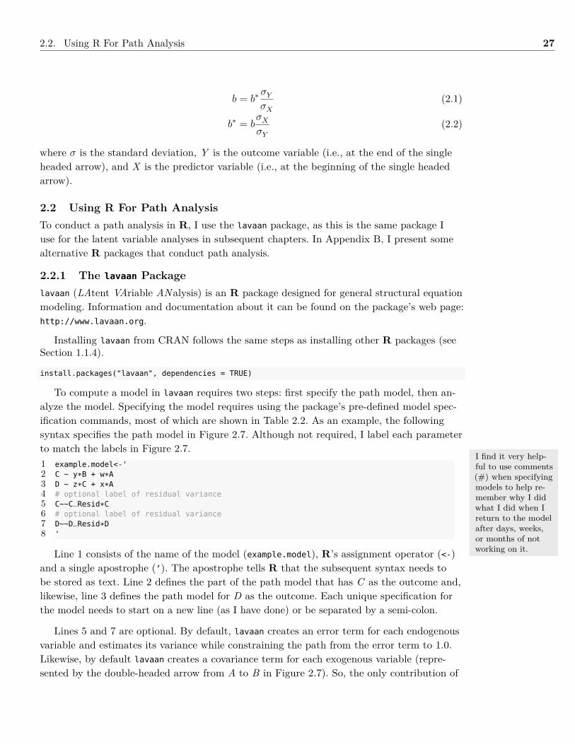
To compute a model in lavaan requires two steps: first specify the path model, then an-alyze the model. Specifying the model requires using the package’s pre-defined model spec-ification commands, most of which are shown in Table 2.2. As an example, the followingsyntax specifies the path model in Figure 2.7. Although not required, I label each parameterto match the labels in Figure 2.7.1 example.model<-'2 C ~ y*B + w*A3 D ~ z*C + x*A4 # optional label of residual variance5 C~~C_Resid*C6 # optional label of residual variance7 D~~D_Resid*D8 '
Line 1 consists of the name of the model (example.model), R’s assignment operator (<-)and a single apostrophe (’). The apostrophe tells R that the subsequent syntax needs tobe stored as text. Line 2 defines the part of the path model that has C as the outcome and,likewise, line 3 defines the path model for D as the outcome. Each unique specification forthe model needs to start on a new line (as I have done) or be separated by a semi-colon.
Lines 5 and 7 are optional. By default, lavaan creates an error term for each endogenousvariable and estimates its variance while constraining the path from the error term to 1.0.Likewise, by default lavaan creates a covariance term for each exogenous variable (repre-sented by the double-headed arrow from A to B in Figure 2.7). So, the only contribution of
I find it very help-ful to use comments(#) when specifyingmodels to help re-member why I didwhat I did when Ireturn to the modelafter days, weeks,or months of notworking on it.
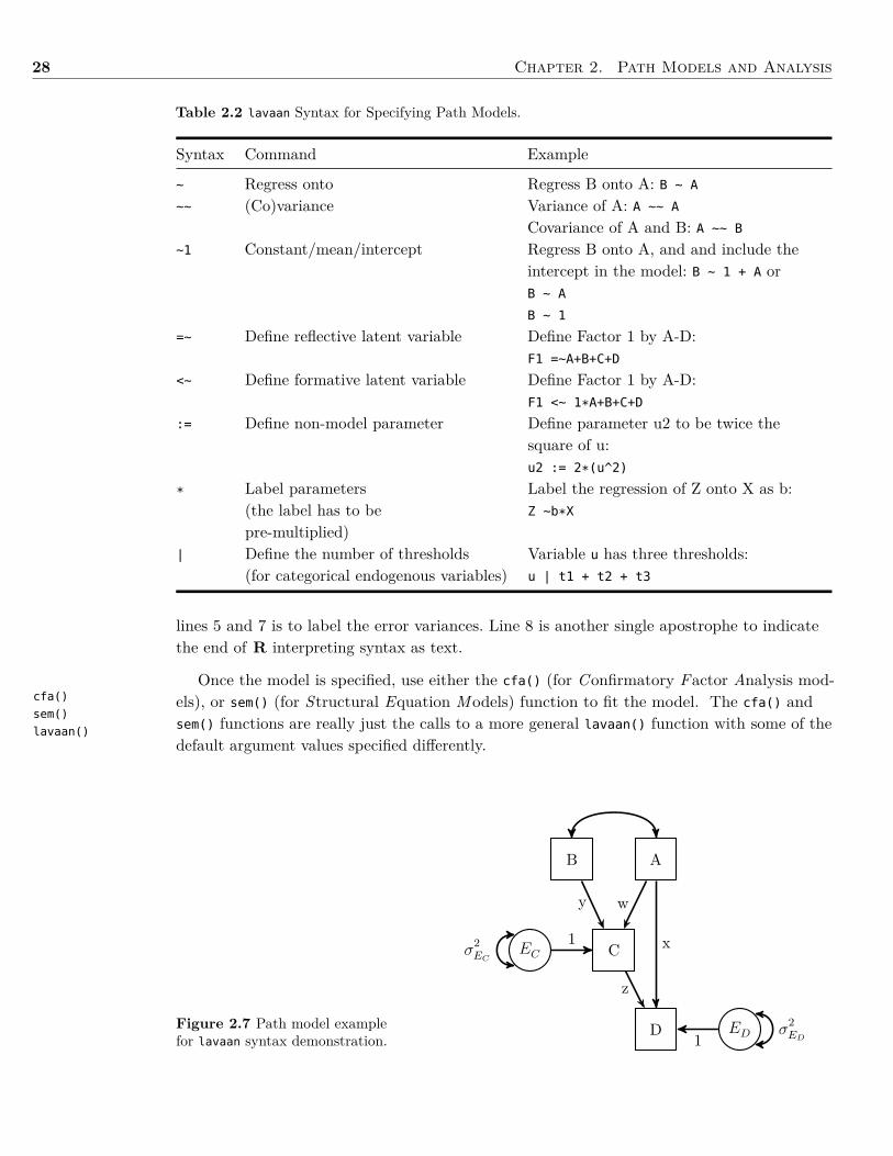
28 Chapter 2. Path Models and Analysis
Table 2.2 lavaan Syntax for Specifying Path Models.
Syntax Command Example
~ Regress onto Regress B onto A: B ~ A
~~ (Co)variance Variance of A: A ~~ A
Covariance of A and B: A ~~ B
~1 Constant/mean/intercept Regress B onto A, and and include theintercept in the model: B ~ 1 + A orB ~ A
B ~ 1
=~ Define reflective latent variable Define Factor 1 by A-D:F1 =~A+B+C+D
<~ Define formative latent variable Define Factor 1 by A-D:F1 <~ 1*A+B+C+D
:= Define non-model parameter Define parameter u2 to be twice thesquare of u:u2 := 2*(u^2)
* Label parameters Label the regression of Z onto X as b:(the label has to be Z ~b*X
pre-multiplied)| Define the number of thresholds Variable u has three thresholds:
(for categorical endogenous variables) u | t1 + t2 + t3
cfa()
sem()
lavaan()
lines 5 and 7 is to label the error variances. Line 8 is another single apostrophe to indicatethe end of R interpreting syntax as text.
Once the model is specified, use either the cfa() (for Confirmatory Factor Analysis mod-els), or sem() (for Structural Equation Models) function to fit the model. The cfa() andsem() functions are really just the calls to a more general lavaan() function with some of thedefault argument values specified differently.
Figure 2.7 Path model examplefor lavaan syntax demonstration.
B A
C
D
EC
ED
y w
x
z
1
1
σ2EC
σ2ED
2.3. Example: Path Analysis using lavaan 29
lavaan accepts either a covariance matrix (and sample size) or raw data as input, usingthe sample.cov (and sample.nobs) or data arguments, respectively. When using a covariancematrix as input, there is an option to also input a mean vector with the sample.mean argu-ment. By default, lavaan uses normal-theory maximum likelihood as the parameter estima-tion technique for models with continuous variables as indicators (the typical model), butother estimators are available.
As an example, say I collected data from 500 individuals on variables A-D used for thepath model in Figure 2.7 that I specified in example.model. Further, suppose I already im-ported the data into R and named it example.data. To estimate the parameters specified inexample.model using example.data, I would use this call to lavaan:
example.fit <- sem(example.model, data = example.data)
If I wanted to use the variables’ covariance matrix (named example.cov) instead of the rawdata, I would use this call to lavaan:
example.fit <- sem(example.model, sample.cov = example.cov, sample.nobs = 500)
Both calls return nothing on-screen because the the results are stored in the example.fit
object. To obtain the lavann results, one option is to use the summary() function.
summary(example.fit)
By default, lavaan’s summary() function returns: (a) a note indicating if the parameter es-timation algorithm converged; (b) the sample size; (c) estimator; (d) fit statistic (χ2) and itsdegrees of freedom and p-value; (e) the unstandardized parameter estimates; (f) the parame-ter estimates’ standard errors; (g) the ratio of the parameter estimates and their standard er-rors, (i.e., Wald statistic); and (h) the p-value for the Wald statistic. The summary() functionhas these default specifications for its arguments: standardized=FALSE, fit.measures=FALSE,
rsquare=FALSE, and modindices=FALSE. Setting standardized=TRUE will include standardizedestimates in the results, setting fit.measures=TRUE will include fit indices in the results (seeAppendix A for a list and description), setting rsquare=TRUE will include the R2 for eachendogenous variable, and setting modindices=TRUE will include modification indices (see Chap-ter 3).
2.3 Example: Path Analysis using lavaan
As a numerical example of using lavaan, I check the parameter estimate values I calculatedin Section 2.1.4. First, I input the covariance matrix in Table 2.1 (see Section 1.1.5.4). Next,I label the rows and columns; otherwise, lavaan does not know where to find the correct(co)variances.
# create a correlation matrixlibrary(lavaan)regression.cor <- lower2full(c(1.0,0.20,1,0.24,0.30,1,0.70,0.80,0.30,1))# name the variables in the matrixcolnames(regression.cor) <- rownames(regression.cor) <- c("X1", "X2", "X3", "Y")regression.cor
To obtain the de-fault values for thecfa() or sem() func-tions, as well astheir various argu-ments and availableestimators, type?cfa or ?sem, respec-tively.
summary()
Many packages havetheir own summary()
functions. The cor-rect one is calledbased on the func-tion that created theobject.
I typically name myR objects with anextension that givestheir type, e.g.: acovariance matrixhas a .cov extension;a correlation matrix:.cor ; a mean vector:.mean; and a SDvector: .sd.
30 Chapter 2. Path Models and Analysis
sem()
Indirect Effect
## X1 X2 X3 Y## X1 1.00 0.2 0.24 0.7## X2 0.20 1.0 0.30 0.8## X3 0.24 0.3 1.00 0.3## Y 0.70 0.8 0.30 1.0
Next, I specify the path model.
regression.model<-'# structural model for YY ~ a*X1 + b*X2 + c*X3# label the residual variance of YY ~~ z*Y'
Last, I estimate the parameters using the sem() function, assuming the n = 1000.
library(lavaan)regression.fit <- sem(regression.model, sample.cov = regression.cor, sample.nobs = 1000)summary(regression.fit, rsquare = TRUE)
## lavaan (0.5-16) converged normally after 25 iterations#### Number of observations 1000#### Estimator ML## Minimum Function Test Statistic 0.000## Degrees of freedom 0## P-value (Chi-square) 1.000#### Parameter estimates:#### Information Expected## Standard Errors Standard#### Estimate Std.err Z-value P(>|z|)## Regressions:## Y ~## X1 (a) 0.571 0.008 74.539 0.000## X2 (b) 0.700 0.008 89.724 0.000## X3 (c) -0.047 0.008 -5.980 0.000#### Variances:## Y (z) 0.054 0.002#### R-Square:#### Y 0.946
Notice that the coefficients in the Estimate column agree with what I found by hand, withinrounding error.
2.4 Indirect EffectAll the models I have shown thus far have been concerned with direct effects of one variableon another. Another type of effect a variable can have is an indirect effect. An indirecteffect is the influence one variable has on another variable, through a second (or third, or
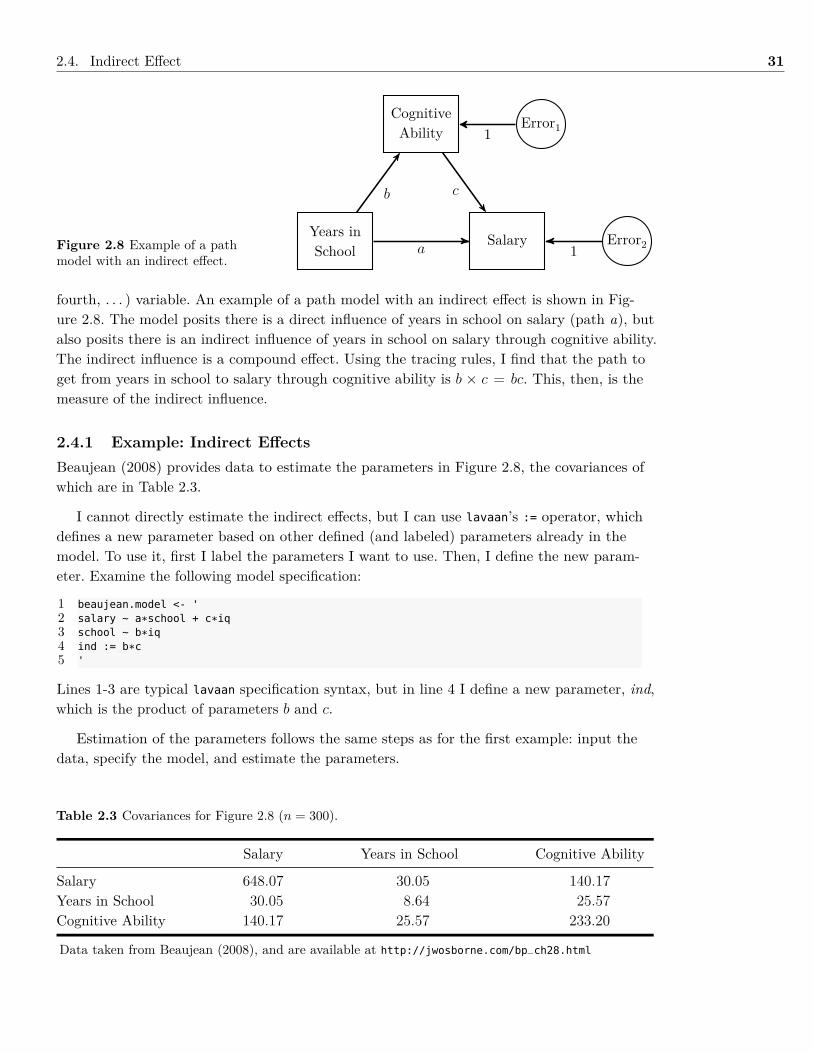
2.4. Indirect Effect 31
Figure 2.8 Example of a pathmodel with an indirect effect.
SalaryYears inSchool
Error2
CognitiveAbility
Error1
a
b c
1
1
fourth, . . . ) variable. An example of a path model with an indirect effect is shown in Fig-ure 2.8. The model posits there is a direct influence of years in school on salary (path a), butalso posits there is an indirect influence of years in school on salary through cognitive ability.The indirect influence is a compound effect. Using the tracing rules, I find that the path toget from years in school to salary through cognitive ability is b × c = bc. This, then, is themeasure of the indirect influence.
2.4.1 Example: Indirect EffectsBeaujean (2008) provides data to estimate the parameters in Figure 2.8, the covariances ofwhich are in Table 2.3.
I cannot directly estimate the indirect effects, but I can use lavaan’s := operator, whichdefines a new parameter based on other defined (and labeled) parameters already in themodel. To use it, first I label the parameters I want to use. Then, I define the new param-eter. Examine the following model specification:
1 beaujean.model <- '2 salary ~ a*school + c*iq3 school ~ b*iq4 ind := b*c5 '
Lines 1-3 are typical lavaan specification syntax, but in line 4 I define a new parameter, ind,which is the product of parameters b and c.
Estimation of the parameters follows the same steps as for the first example: input thedata, specify the model, and estimate the parameters.
Table 2.3 Covariances for Figure 2.8 (n = 300).
Salary Years in School Cognitive Ability
Salary 648.07 30.05 140.17Years in School 30.05 8.64 25.57Cognitive Ability 140.17 25.57 233.20
Data taken from Beaujean (2008), and are available at http://jwosborne.com/bp_ch28.html
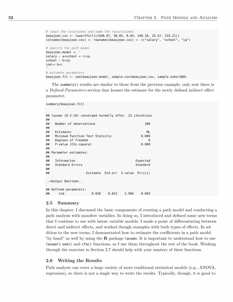
32 Chapter 2. Path Models and Analysis
# input the covarianes and name the rows/columnsbeaujean.cov <- lower2full(c(648.07, 30.05, 8.64, 140.18, 25.57, 233.21))colnames(beaujean.cov) <- rownames(beaujean.cov) <- c("salary", "school", "iq")
# specify the path modelbeaujean.model <- 'salary ~ a*school + c*iqschool ~ b*iqind:= b*c'# estimate parametersbeaujean.fit <- sem(beaujean.model, sample.cov=beaujean.cov, sample.nobs=300)
The summary() results are similar to those from the previous example, only now there isa Defined Parameters section that houses the estimate for the newly defined indirect effectparameter.
summary(beaujean.fit)
## lavaan (0.5-16) converged normally after 23 iterations#### Number of observations 300#### Estimator ML## Minimum Function Test Statistic 0.000## Degrees of freedom 0## P-value (Chi-square) 0.000#### Parameter estimates:#### Information Expected## Standard Errors Standard#### Estimate Std.err Z-value P(>|z|)
..<Output Omitted>..
## Defined parameters:## ind 0.036 0.012 2.984 0.003
2.5 SummaryIn this chapter, I discussed the basic components of creating a path model and conducting apath analysis with manifest variables. In doing so, I introduced and defined some new termsthat I continue to use with latent variable models. I made a point of differentiating betweendirect and indirect effects, and worked though examples with both types of effects. In ad-dition to the new terms, I demonstrated how to estimate the coefficients in a path model“by hand” as well by using the R package lavaan. It is important to understand how to uselavaan’s sem() and cfa() functions, as I use them throughout the rest of the book. Workingthrough the exercises in Section 2.7 should help with your mastery of these functions.
2.6 Writing the ResultsPath analysis can cover a large variety of more traditional statistical models (e.g., ANOVA,regression), so there is not a single way to write the results. Typically, though, it is good to
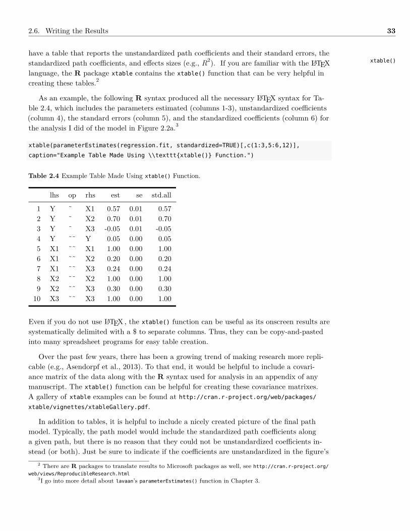
2.6. Writing the Results 33
have a table that reports the unstandardized path coefficients and their standard errors, thestandardized path coefficients, and effects sizes (e.g., R2). If you are familiar with the LATEXlanguage, the R package xtable contains the xtable() function that can be very helpful increating these tables.2
As an example, the following R syntax produced all the necessary LATEX syntax for Ta-ble 2.4, which includes the parameters estimated (columns 1-3), unstandardized coefficients(column 4), the standard errors (column 5), and the standardized coefficients (column 6) forthe analysis I did of the model in Figure 2.2a.3
xtable(parameterEstimates(regression.fit, standardized=TRUE)[,c(1:3,5:6,12)],
caption="Example Table Made Using \\texttt{xtable()} Function.")
Table 2.4 Example Table Made Using xtable() Function.
lhs op rhs est se std.all
1 Y ˜ X1 0.57 0.01 0.572 Y ˜ X2 0.70 0.01 0.703 Y ˜ X3 -0.05 0.01 -0.054 Y ˜˜ Y 0.05 0.00 0.055 X1 ˜˜ X1 1.00 0.00 1.006 X1 ˜˜ X2 0.20 0.00 0.207 X1 ˜˜ X3 0.24 0.00 0.248 X2 ˜˜ X2 1.00 0.00 1.009 X2 ˜˜ X3 0.30 0.00 0.3010 X3 ˜˜ X3 1.00 0.00 1.00
Even if you do not use LATEX , the xtable() function can be useful as its onscreen results aresystematically delimited with a $ to separate columns. Thus, they can be copy-and-pastedinto many spreadsheet programs for easy table creation.
Over the past few years, there has been a growing trend of making research more repli-cable (e.g., Asendorpf et al., 2013). To that end, it would be helpful to include a covari-ance matrix of the data along with the R syntax used for analysis in an appendix of anymanuscript. The xtable() function can be helpful for creating these covariance matrixes.A gallery of xtable examples can be found at http://cran.r-project.org/web/packages/
xtable/vignettes/xtableGallery.pdf.
In addition to tables, it is helpful to include a nicely created picture of the final pathmodel. Typically, the path model would include the standardized path coefficients alonga given path, but there is no reason that they could not be unstandardized coefficients in-stead (or both). Just be sure to indicate if the coefficients are unstandardized in the figure’s
xtable()
2 There are R packages to translate results to Microsoft packages as well, see http://cran.r-project.org/
web/views/ReproducibleResearch.html3I go into more detail about lavaan’s parameterEstimates() function in Chapter 3.
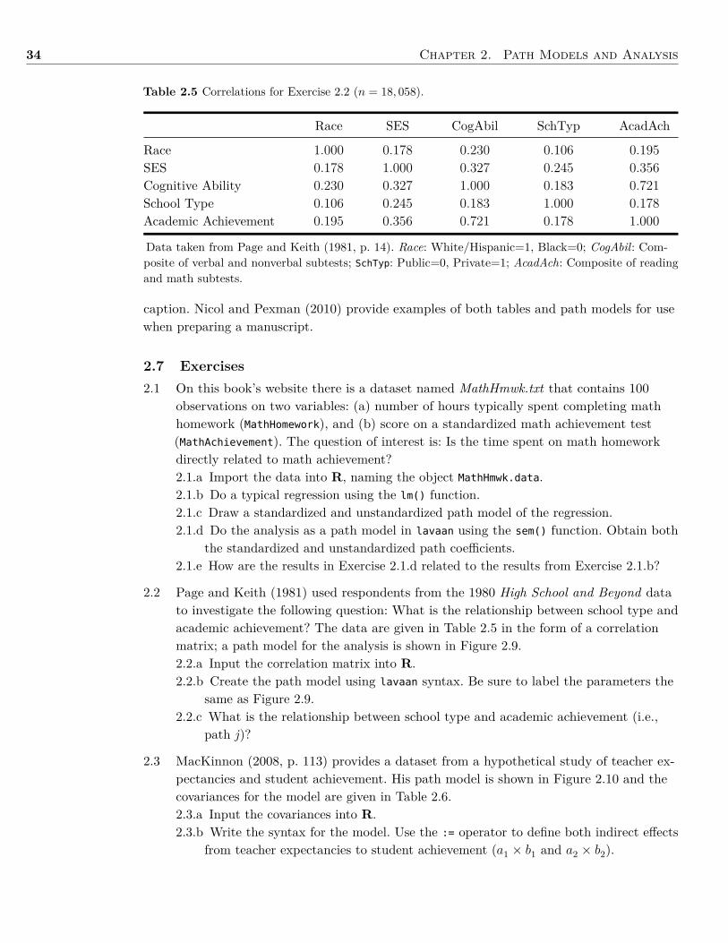
34 Chapter 2. Path Models and Analysis
Table 2.5 Correlations for Exercise 2.2 (n = 18, 058).
Race SES CogAbil SchTyp AcadAch
Race 1.000 0.178 0.230 0.106 0.195SES 0.178 1.000 0.327 0.245 0.356Cognitive Ability 0.230 0.327 1.000 0.183 0.721School Type 0.106 0.245 0.183 1.000 0.178Academic Achievement 0.195 0.356 0.721 0.178 1.000
Data taken from Page and Keith (1981, p. 14). Race: White/Hispanic=1, Black=0; CogAbil: Com-posite of verbal and nonverbal subtests; SchTyp: Public=0, Private=1; AcadAch: Composite of readingand math subtests.
caption. Nicol and Pexman (2010) provide examples of both tables and path models for usewhen preparing a manuscript.
2.7 Exercises2.1 On this book’s website there is a dataset named MathHmwk.txt that contains 100
observations on two variables: (a) number of hours typically spent completing mathhomework (MathHomework), and (b) score on a standardized math achievement test(MathAchievement). The question of interest is: Is the time spent on math homeworkdirectly related to math achievement?2.1.a Import the data into R, naming the object MathHmwk.data.2.1.b Do a typical regression using the lm() function.2.1.c Draw a standardized and unstandardized path model of the regression.2.1.d Do the analysis as a path model in lavaan using the sem() function. Obtain both
the standardized and unstandardized path coefficients.2.1.e How are the results in Exercise 2.1.d related to the results from Exercise 2.1.b?
2.2 Page and Keith (1981) used respondents from the 1980 High School and Beyond datato investigate the following question: What is the relationship between school type andacademic achievement? The data are given in Table 2.5 in the form of a correlationmatrix; a path model for the analysis is shown in Figure 2.9.2.2.a Input the correlation matrix into R.2.2.b Create the path model using lavaan syntax. Be sure to label the parameters the
same as Figure 2.9.2.2.c What is the relationship between school type and academic achievement (i.e.,
path j)?
2.3 MacKinnon (2008, p. 113) provides a dataset from a hypothetical study of teacher ex-pectancies and student achievement. His path model is shown in Figure 2.10 and thecovariances for the model are given in Table 2.6.2.3.a Input the covariances into R.2.3.b Write the syntax for the model. Use the := operator to define both indirect effects
from teacher expectancies to student achievement (a1 × b1 and a2 × b2).
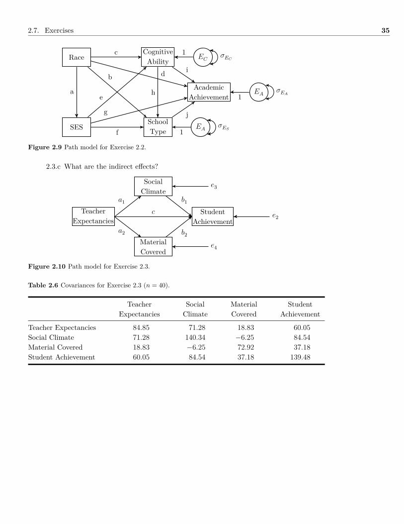
2.7. Exercises 35
Race
SES
CognitiveAbility
SchoolType
AcademicAchievement
EA
EA
EC
σEA
σES
σEC
a
b
c
d
e
f
g
h
i
j
1
1
1
Figure 2.9 Path model for Exercise 2.2.
2.3.c What are the indirect effects?
TeacherExpectancies
SocialClimate
MaterialCovered
StudentAchievement
e3
e4
e2
a1
a2
b1
b2
c
Figure 2.10 Path model for Exercise 2.3.
Table 2.6 Covariances for Exercise 2.3 (n = 40).
Teacher Social Material StudentExpectancies Climate Covered Achievement
Teacher Expectancies 84.85 71.28 18.83 60.05Social Climate 71.28 140.34 −6.25 84.54Material Covered 18.83 −6.25 72.92 37.18Student Achievement 60.05 84.54 37.18 139.48

36 Chapter 2. Path Models and Analysis
2.8 References & Further ReadingsAsendorpf, J. B., Conner, M., De Fruyt, F., De Houwer, J., Denissen, J. J. A., Fiedler, K., . . .
Wicherts, J. M. (2013). Recommendations for increasing replicability in psychology.European Journal of Personality, 27 , 108-119. doi: 10.1002/per.1919
Beaujean, A. A. (2008). Mediation, moderation, and the study of individual differences. InJ. W. Osborne (Ed.), Best practices in quantitative methods (pp. 422–442). ThousandOaks, CA: Sage.
Boker, S. M., & McArdle, J. J. (2005). Path analysis and path diagrams. In B. Everitt &D. C. Howell (Eds.), Encyclopedia of behavioral statistics (Vol. 3, pp. 1529–1531). WestSussex, England: Wiley.
MacKinnon, D. P. (2008). Introduction to statistical mediation analysis. Mahwah, NJ:Erlbaum.
Nicol, A. A. M., & Pexman, P. M. (2010). Presenting your findings: A practical guide forcreating tables (6th ed.). Washington, DC: American Psychological Association.
Page, E. B., & Keith, T. Z. (1981). Effects of U.S. private schools: A technical analysis of tworecent claims. Educational Researcher , 10 , 7-17. doi: 10.2307/1174256
Rosseel, Y. (2012). lavaan: An R package for structural equation modeling. Journal ofStatistical Software, 48 (2), 1-36. Retrieved from www.jstatsoft.org/v48/i02/.
Wolfle, L. M. (1999). Sewall Wright on the method of path coefficients: An annotatedbibliography. Structural Equation Modeling: A Multidisciplinary Journal, 6 , 280-291. doi:10.1080/10705519909540134
Wolfle, L. M. (2003). The introduction of path analysis to the social sciences, and someemergent themes: An annotated bibliography. Structural Equation Modeling: AMultidisciplinary Journal, 10 , 1-34. doi: 10.1207/S15328007SEM1001_1
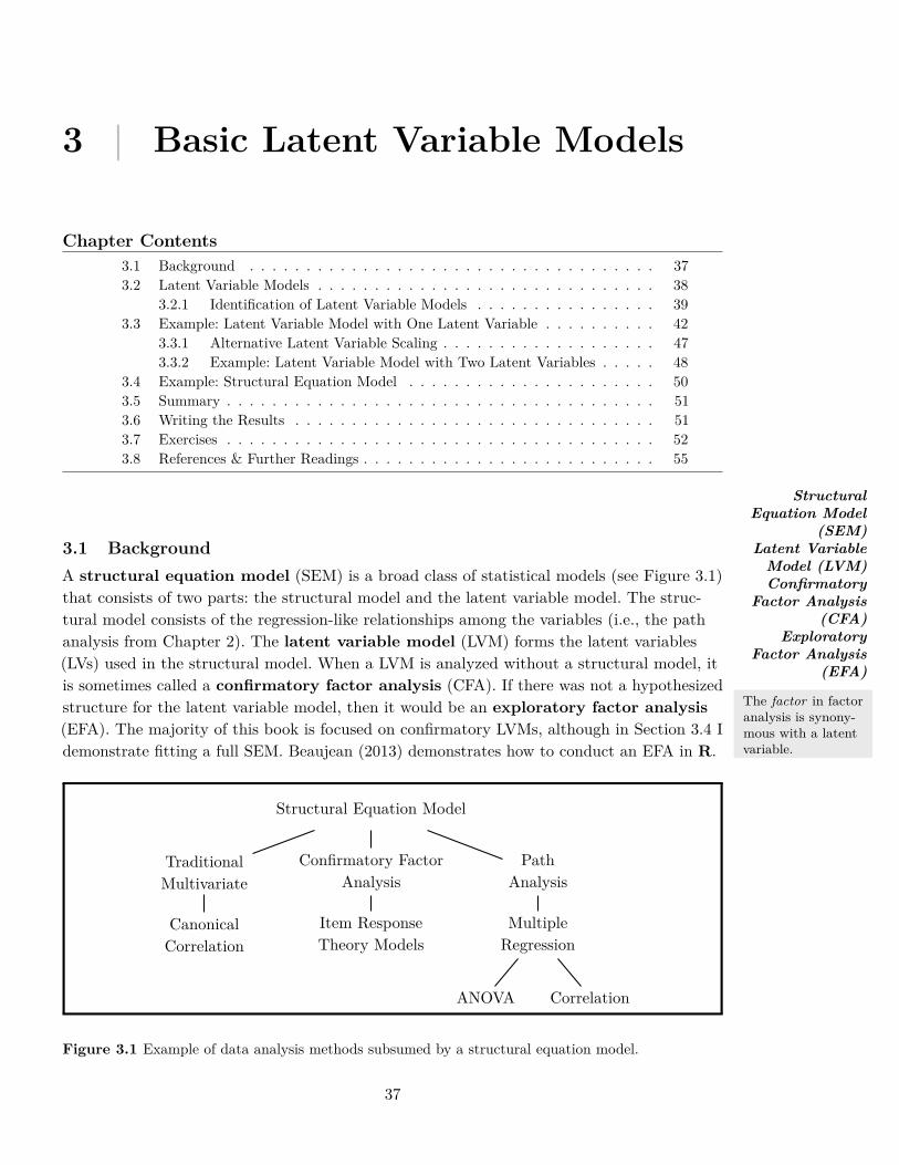
3 | Basic Latent Variable Models
Chapter Contents3.1 Background . . . . . . . . . . . . . . . . . . . . . . . . . . . . . . . . . . . . 373.2 Latent Variable Models . . . . . . . . . . . . . . . . . . . . . . . . . . . . . . 38
3.2.1 Identification of Latent Variable Models . . . . . . . . . . . . . . . . 393.3 Example: Latent Variable Model with One Latent Variable . . . . . . . . . . 42
3.3.1 Alternative Latent Variable Scaling . . . . . . . . . . . . . . . . . . . 473.3.2 Example: Latent Variable Model with Two Latent Variables . . . . . 48
3.4 Example: Structural Equation Model . . . . . . . . . . . . . . . . . . . . . . 503.5 Summary . . . . . . . . . . . . . . . . . . . . . . . . . . . . . . . . . . . . . . 513.6 Writing the Results . . . . . . . . . . . . . . . . . . . . . . . . . . . . . . . . 513.7 Exercises . . . . . . . . . . . . . . . . . . . . . . . . . . . . . . . . . . . . . . 523.8 References & Further Readings . . . . . . . . . . . . . . . . . . . . . . . . . . 55
3.1 BackgroundA structural equation model (SEM) is a broad class of statistical models (see Figure 3.1)that consists of two parts: the structural model and the latent variable model. The struc-tural model consists of the regression-like relationships among the variables (i.e., the pathanalysis from Chapter 2). The latent variable model (LVM) forms the latent variables(LVs) used in the structural model. When a LVM is analyzed without a structural model, itis sometimes called a confirmatory factor analysis (CFA). If there was not a hypothesizedstructure for the latent variable model, then it would be an exploratory factor analysis(EFA). The majority of this book is focused on confirmatory LVMs, although in Section 3.4 Idemonstrate fitting a full SEM. Beaujean (2013) demonstrates how to conduct an EFA in R.
StructuralEquation Model
(SEM)Latent VariableModel (LVM)Confirmatory
Factor Analysis(CFA)
ExploratoryFactor Analysis
(EFA)
The factor in factoranalysis is synony-mous with a latentvariable.
Structural Equation Model
TraditionalMultivariate
CanonicalCorrelation
Confirmatory FactorAnalysis
Item ResponseTheory Models
PathAnalysis
MultipleRegression
ANOVA Correlation
Figure 3.1 Example of data analysis methods subsumed by a structural equation model.
37
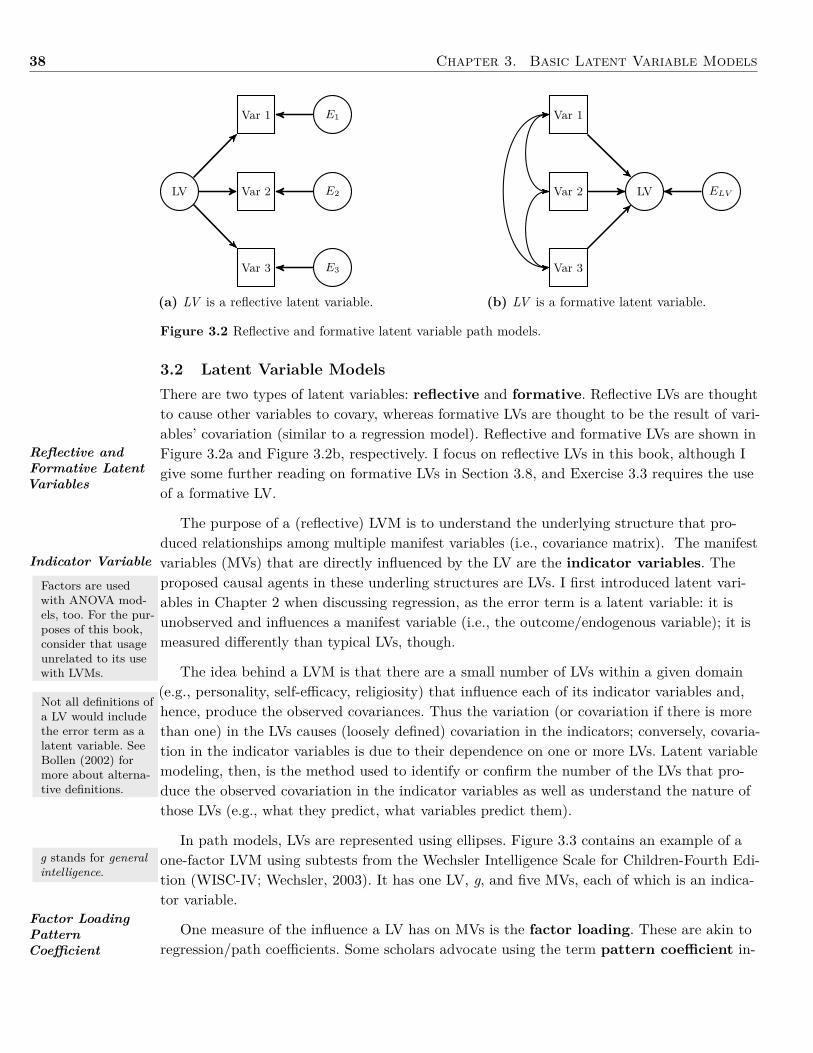
38 Chapter 3. Basic Latent Variable Models
LV Var 2
Var 3
Var 1 E1
E2
E3
(a) LV is a reflective latent variable.
LVVar 2
Var 3
Var 1
ELV
(b) LV is a formative latent variable.
Figure 3.2 Reflective and formative latent variable path models.
Reflective andFormative LatentVariables
Indicator Variable
Factors are usedwith ANOVA mod-els, too. For the pur-poses of this book,consider that usageunrelated to its usewith LVMs.
Not all definitions ofa LV would includethe error term as alatent variable. SeeBollen (2002) formore about alterna-tive definitions.
g stands for generalintelligence.
Factor LoadingPatternCoefficient
3.2 Latent Variable ModelsThere are two types of latent variables: reflective and formative. Reflective LVs are thoughtto cause other variables to covary, whereas formative LVs are thought to be the result of vari-ables’ covariation (similar to a regression model). Reflective and formative LVs are shown inFigure 3.2a and Figure 3.2b, respectively. I focus on reflective LVs in this book, although Igive some further reading on formative LVs in Section 3.8, and Exercise 3.3 requires the useof a formative LV.
The purpose of a (reflective) LVM is to understand the underlying structure that pro-duced relationships among multiple manifest variables (i.e., covariance matrix). The manifestvariables (MVs) that are directly influenced by the LV are the indicator variables. Theproposed causal agents in these underling structures are LVs. I first introduced latent vari-ables in Chapter 2 when discussing regression, as the error term is a latent variable: it isunobserved and influences a manifest variable (i.e., the outcome/endogenous variable); it ismeasured differently than typical LVs, though.
The idea behind a LVM is that there are a small number of LVs within a given domain(e.g., personality, self-efficacy, religiosity) that influence each of its indicator variables and,hence, produce the observed covariances. Thus the variation (or covariation if there is morethan one) in the LVs causes (loosely defined) covariation in the indicators; conversely, covaria-tion in the indicator variables is due to their dependence on one or more LVs. Latent variablemodeling, then, is the method used to identify or confirm the number of the LVs that pro-duce the observed covariation in the indicator variables as well as understand the nature ofthose LVs (e.g., what they predict, what variables predict them).
In path models, LVs are represented using ellipses. Figure 3.3 contains an example of aone-factor LVM using subtests from the Wechsler Intelligence Scale for Children-Fourth Edi-tion (WISC-IV; Wechsler, 2003). It has one LV, g, and five MVs, each of which is an indica-tor variable.
One measure of the influence a LV has on MVs is the factor loading. These are akin toregression/path coefficients. Some scholars advocate using the term pattern coefficient in-
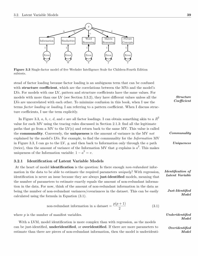
3.2. Latent Variable Models 39
g
WordReasoningSimilaritiesInformation
MatrixReasoning
PictureConcepts
Error Error Error Error Error
a b cd e
1 1 1 1 1
v w x y z
Figure 3.3 Single-factor model of five Wechsler Intelligence Scale for Children-Fourth Editionsubtests.
stead of factor loading because factor loading is an ambiguous term that can be confusedwith structure coefficient, which are the correlations between the MVs and the model’sLVs. For models with one LV, pattern and structure coefficients have the same values. Formodels with more than one LV (see Section 3.3.2), they have different values unless all theLVs are uncorrelated with each other. To minimize confusion in this book, when I use theterms factor loading or loading, I am referring to a pattern coefficient. When I discuss struc-ture coefficients, I use the term explicitly.
In Figure 3.3, a, b, c, d, and e are all factor loadings. I can obtain something akin to a R2
value for each MV using the tracing rules discussed in Section 2.1.3: find all the legitimatepaths that go from a MV to the LV(s) and return back to the same MV. This value is calledthe communality. Conversely, the uniqueness is the amount of variance in the MV notexplained by the model’s LVs. For example, to find the communality for the Information MVin Figure 3.3, I can go to the LV, g, and then back to Information only through the a path(twice), thus the amount of variance of the Information MV that g explains is a2. This makesuniqueness of the Information variable: 1− a2 = v.
3.2.1 Identification of Latent Variable ModelsAt the heart of model identification is the question: Is there enough non-redundant infor-mation in the data to be able to estimate the required parameters uniquely? With regression,identification is never an issue because they are always just-identified models, meaning thatthe number of parameters to estimate exactly equals the amount of non-redundant informa-tion in the data. For now, think of the amount of non-redundant information in the data asbeing the number of non-redundant variances/covariances in the dataset. This can be easilycalculated using the formula in Equation (3.1).
non-redundant information in a dataset = p(p+ 1)2 (3.1)
where p is the number of manifest variables.
With a LVM, model identification is more complex than with regression, as the modelscan be just-identified, underidentified, or overidentified. If there are more parameters toestimate than there are pieces of non-redundant information, then the model is underidenti-
StructureCoefficient
Communality
Uniqueness
Identification ofLatent Variable
Just-IdentifiedModel
UnderidentifiedModel
OveridentifiedModel
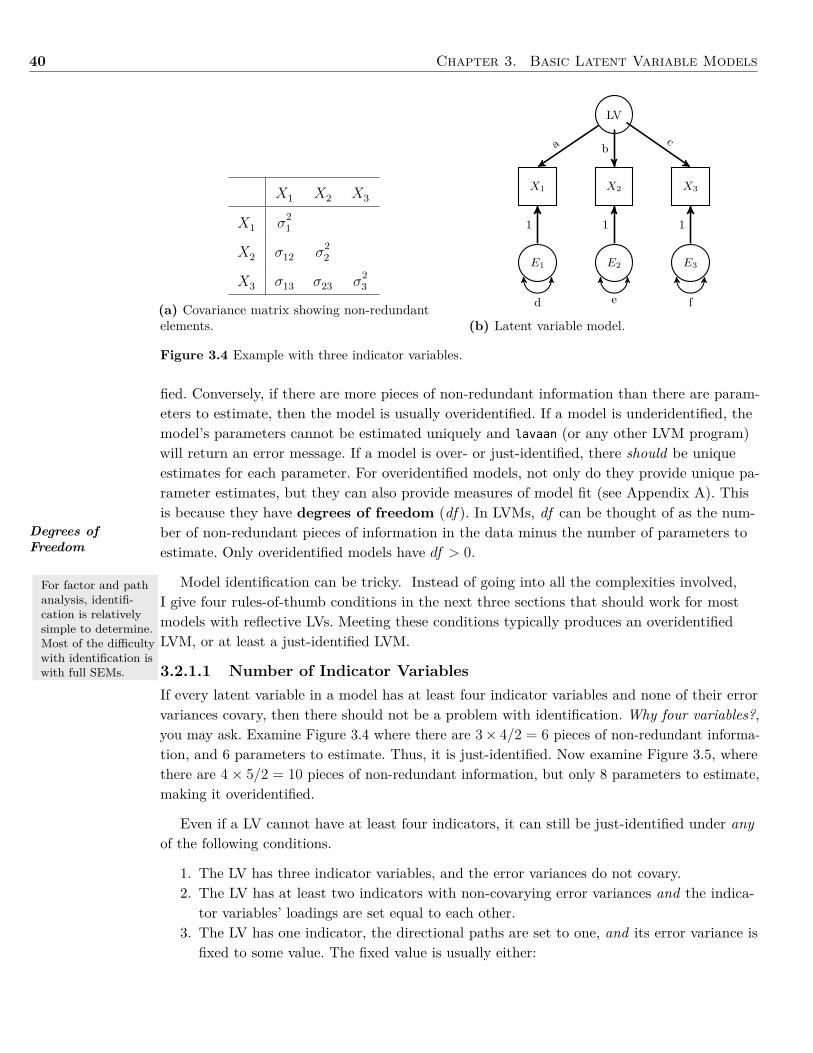
40 Chapter 3. Basic Latent Variable Models
X1 X2 X3
X1 σ21
X2 σ12 σ22
X3 σ13 σ23 σ23
(a) Covariance matrix showing non-redundantelements.
LV
X2 X3X1
E1 E2 E3
a bc
1 1 1
d e f
(b) Latent variable model.
Figure 3.4 Example with three indicator variables.
Degrees ofFreedom
For factor and pathanalysis, identifi-cation is relativelysimple to determine.Most of the difficultywith identification iswith full SEMs.
fied. Conversely, if there are more pieces of non-redundant information than there are param-eters to estimate, then the model is usually overidentified. If a model is underidentified, themodel’s parameters cannot be estimated uniquely and lavaan (or any other LVM program)will return an error message. If a model is over- or just-identified, there should be uniqueestimates for each parameter. For overidentified models, not only do they provide unique pa-rameter estimates, but they can also provide measures of model fit (see Appendix A). Thisis because they have degrees of freedom (df ). In LVMs, df can be thought of as the num-ber of non-redundant pieces of information in the data minus the number of parameters toestimate. Only overidentified models have df > 0.
Model identification can be tricky. Instead of going into all the complexities involved,I give four rules-of-thumb conditions in the next three sections that should work for mostmodels with reflective LVs. Meeting these conditions typically produces an overidentifiedLVM, or at least a just-identified LVM.
3.2.1.1 Number of Indicator VariablesIf every latent variable in a model has at least four indicator variables and none of their errorvariances covary, then there should not be a problem with identification. Why four variables?,you may ask. Examine Figure 3.4 where there are 3× 4/2 = 6 pieces of non-redundant informa-tion, and 6 parameters to estimate. Thus, it is just-identified. Now examine Figure 3.5, wherethere are 4× 5/2 = 10 pieces of non-redundant information, but only 8 parameters to estimate,making it overidentified.
Even if a LV cannot have at least four indicators, it can still be just-identified under anyof the following conditions.
1. The LV has three indicator variables, and the error variances do not covary.2. The LV has at least two indicators with non-covarying error variances and the indica-
tor variables’ loadings are set equal to each other.3. The LV has one indicator, the directional paths are set to one, and its error variance is
fixed to some value. The fixed value is usually either:
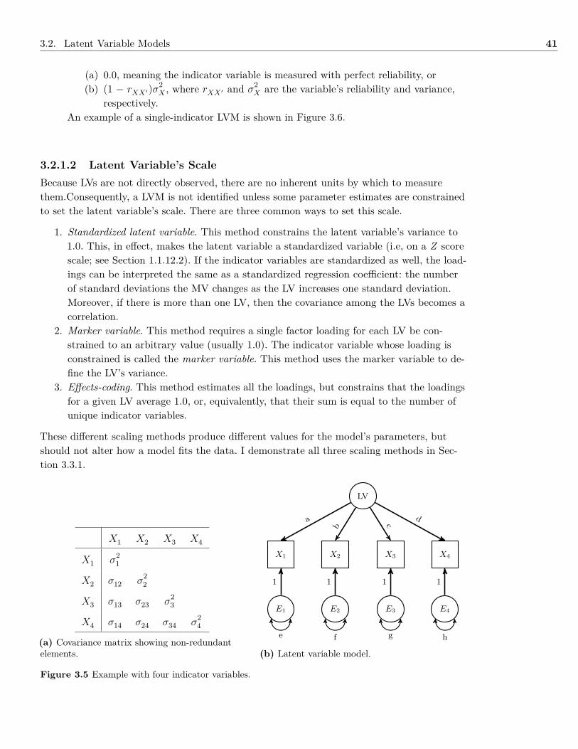
3.2. Latent Variable Models 41
(a) 0.0, meaning the indicator variable is measured with perfect reliability, or(b) (1 − rXX′)σ2
X , where rXX′ and σ2X are the variable’s reliability and variance,
respectively.An example of a single-indicator LVM is shown in Figure 3.6.
3.2.1.2 Latent Variable’s ScaleBecause LVs are not directly observed, there are no inherent units by which to measurethem.Consequently, a LVM is not identified unless some parameter estimates are constrainedto set the latent variable’s scale. There are three common ways to set this scale.
1. Standardized latent variable. This method constrains the latent variable’s variance to1.0. This, in effect, makes the latent variable a standardized variable (i.e, on a Z scorescale; see Section 1.1.12.2). If the indicator variables are standardized as well, the load-ings can be interpreted the same as a standardized regression coefficient: the numberof standard deviations the MV changes as the LV increases one standard deviation.Moreover, if there is more than one LV, then the covariance among the LVs becomes acorrelation.
2. Marker variable. This method requires a single factor loading for each LV be con-strained to an arbitrary value (usually 1.0). The indicator variable whose loading isconstrained is called the marker variable. This method uses the marker variable to de-fine the LV’s variance.
3. Effects-coding. This method estimates all the loadings, but constrains that the loadingsfor a given LV average 1.0, or, equivalently, that their sum is equal to the number ofunique indicator variables.
These different scaling methods produce different values for the model’s parameters, butshould not alter how a model fits the data. I demonstrate all three scaling methods in Sec-tion 3.3.1.
X1 X2 X3 X4
X1 σ21
X2 σ12 σ22
X3 σ13 σ23 σ23
X4 σ14 σ24 σ34 σ24
(a) Covariance matrix showing non-redundantelements.
LV
X2X1 X3 X4
E1 E2 E3 E4
a
b c d
1 1 1 1
e f g h
(b) Latent variable model.
Figure 3.5 Example with four indicator variables.
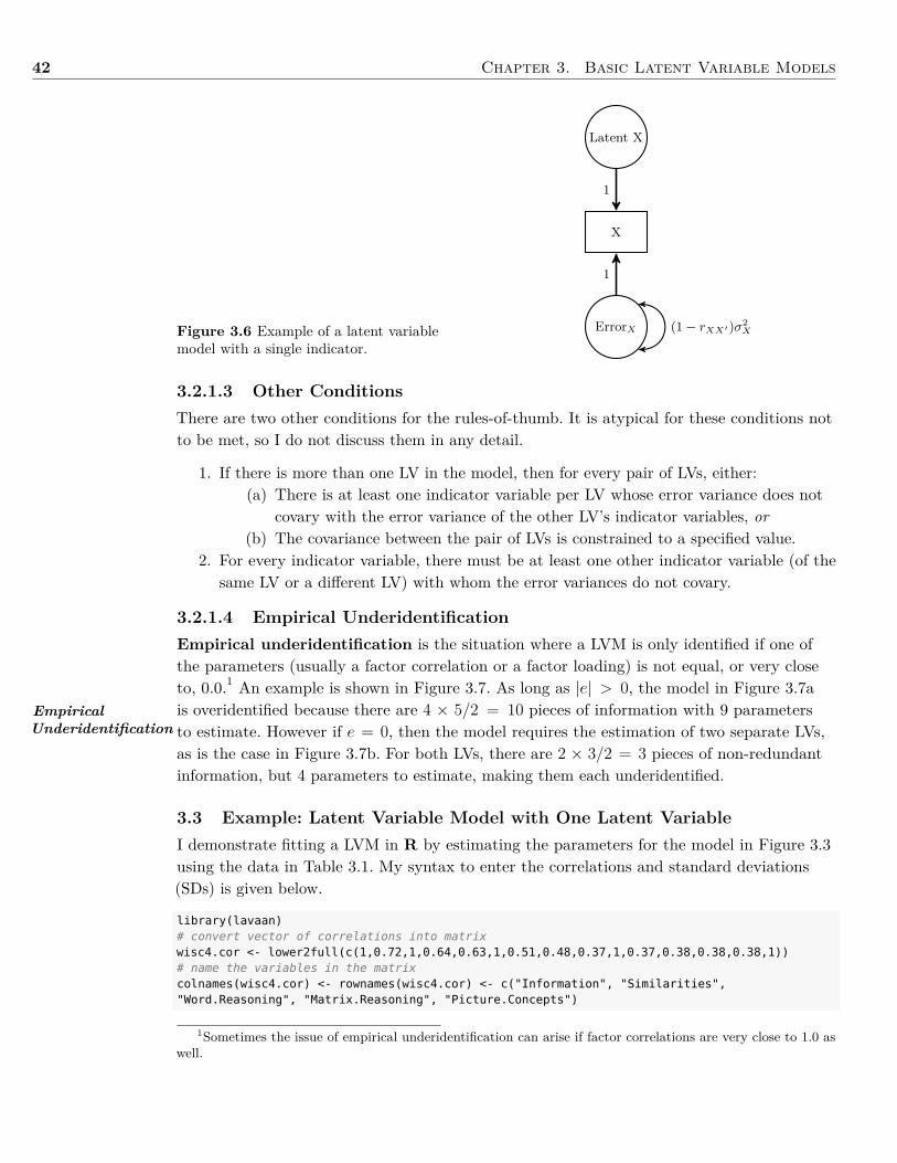
42 Chapter 3. Basic Latent Variable Models
Figure 3.6 Example of a latent variablemodel with a single indicator.
Latent X
X
ErrorX
1
1
(1 − rXX′ )σ2X
EmpiricalUnderidentification
3.2.1.3 Other ConditionsThere are two other conditions for the rules-of-thumb. It is atypical for these conditions notto be met, so I do not discuss them in any detail.
1. If there is more than one LV in the model, then for every pair of LVs, either:(a) There is at least one indicator variable per LV whose error variance does not
covary with the error variance of the other LV’s indicator variables, or(b) The covariance between the pair of LVs is constrained to a specified value.
2. For every indicator variable, there must be at least one other indicator variable (of thesame LV or a different LV) with whom the error variances do not covary.
3.2.1.4 Empirical UnderidentificationEmpirical underidentification is the situation where a LVM is only identified if one ofthe parameters (usually a factor correlation or a factor loading) is not equal, or very closeto, 0.0.1 An example is shown in Figure 3.7. As long as |e| > 0, the model in Figure 3.7ais overidentified because there are 4 × 5/2 = 10 pieces of information with 9 parametersto estimate. However if e = 0, then the model requires the estimation of two separate LVs,as is the case in Figure 3.7b. For both LVs, there are 2 × 3/2 = 3 pieces of non-redundantinformation, but 4 parameters to estimate, making them each underidentified.
3.3 Example: Latent Variable Model with One Latent VariableI demonstrate fitting a LVM in R by estimating the parameters for the model in Figure 3.3using the data in Table 3.1. My syntax to enter the correlations and standard deviations(SDs) is given below.
library(lavaan)# convert vector of correlations into matrixwisc4.cor <- lower2full(c(1,0.72,1,0.64,0.63,1,0.51,0.48,0.37,1,0.37,0.38,0.38,0.38,1))# name the variables in the matrixcolnames(wisc4.cor) <- rownames(wisc4.cor) <- c("Information", "Similarities","Word.Reasoning", "Matrix.Reasoning", "Picture.Concepts")
1Sometimes the issue of empirical underidentification can arise if factor correlations are very close to 1.0 aswell.
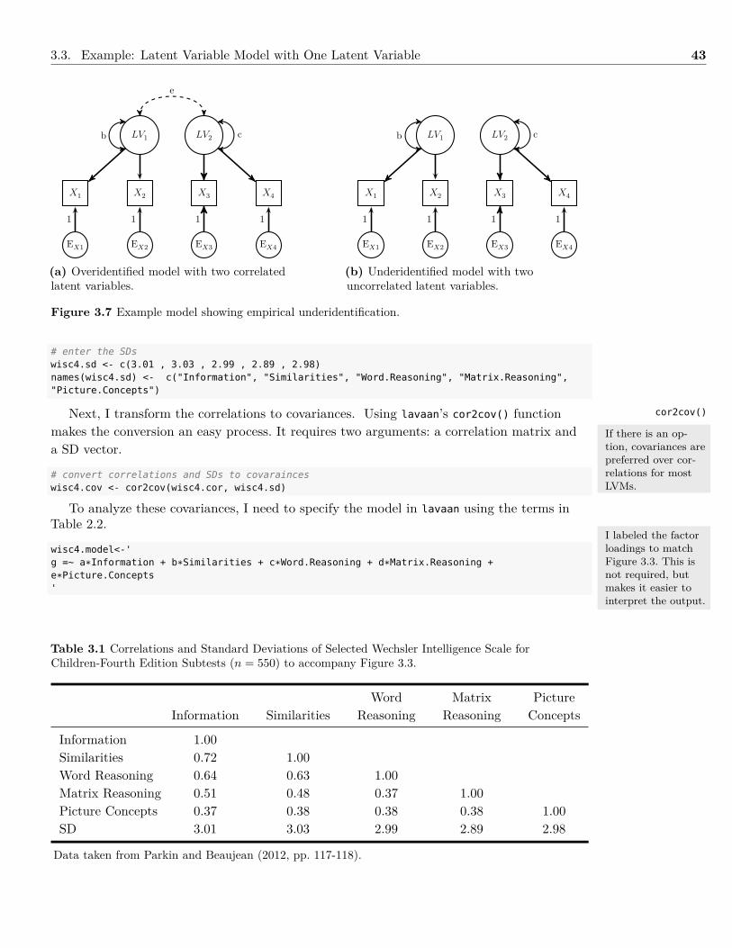
3.3. Example: Latent Variable Model with One Latent Variable 43
X3X2X1 X4
EX1 EX2 EX3 EX4
1 1 1 1
LV1 LV2
e
b c
(a) Overidentified model with two correlatedlatent variables.
X3X2X1 X4
EX1 EX2 EX3 EX4
1 1 1 1
LV1 LV2b c
(b) Underidentified model with twouncorrelated latent variables.
Figure 3.7 Example model showing empirical underidentification.
# enter the SDswisc4.sd <- c(3.01 , 3.03 , 2.99 , 2.89 , 2.98)names(wisc4.sd) <- c("Information", "Similarities", "Word.Reasoning", "Matrix.Reasoning","Picture.Concepts")
Next, I transform the correlations to covariances. Using lavaan’s cor2cov() functionmakes the conversion an easy process. It requires two arguments: a correlation matrix anda SD vector.
# convert correlations and SDs to covarainceswisc4.cov <- cor2cov(wisc4.cor, wisc4.sd)
To analyze these covariances, I need to specify the model in lavaan using the terms inTable 2.2.
wisc4.model<-'g =~ a*Information + b*Similarities + c*Word.Reasoning + d*Matrix.Reasoning +e*Picture.Concepts'
cor2cov()
If there is an op-tion, covariances arepreferred over cor-relations for mostLVMs.
I labeled the factorloadings to matchFigure 3.3. This isnot required, butmakes it easier tointerpret the output.
Table 3.1 Correlations and Standard Deviations of Selected Wechsler Intelligence Scale forChildren-Fourth Edition Subtests (n = 550) to accompany Figure 3.3.
Word Matrix PictureInformation Similarities Reasoning Reasoning Concepts
Information 1.00Similarities 0.72 1.00Word Reasoning 0.64 0.63 1.00Matrix Reasoning 0.51 0.48 0.37 1.00Picture Concepts 0.37 0.38 0.38 0.38 1.00SD 3.01 3.03 2.99 2.89 2.98
Data taken from Parkin and Beaujean (2012, pp. 117-118).
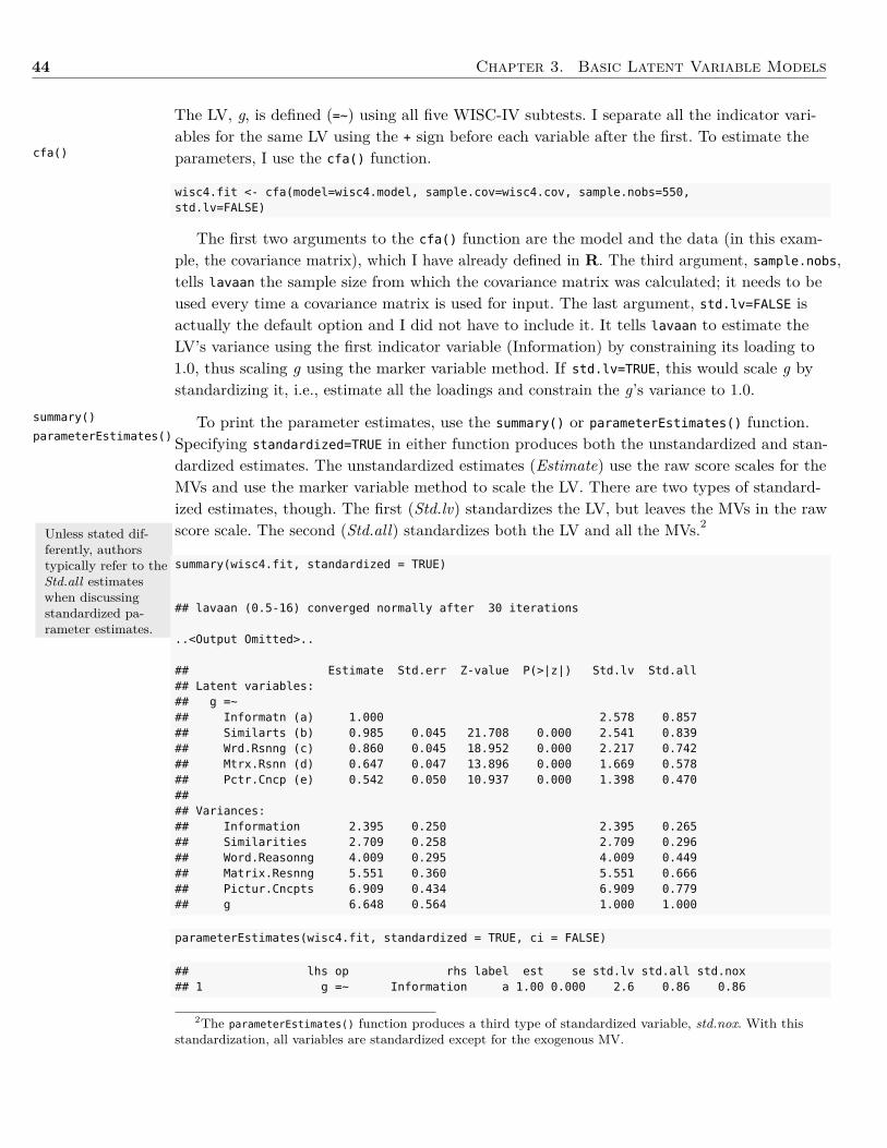
44 Chapter 3. Basic Latent Variable Models
cfa()
summary()
parameterEstimates()
Unless stated dif-ferently, authorstypically refer to theStd.all estimateswhen discussingstandardized pa-rameter estimates.
The LV, g, is defined (=~) using all five WISC-IV subtests. I separate all the indicator vari-ables for the same LV using the + sign before each variable after the first. To estimate theparameters, I use the cfa() function.
wisc4.fit <- cfa(model=wisc4.model, sample.cov=wisc4.cov, sample.nobs=550,std.lv=FALSE)
The first two arguments to the cfa() function are the model and the data (in this exam-ple, the covariance matrix), which I have already defined in R. The third argument, sample.nobs,tells lavaan the sample size from which the covariance matrix was calculated; it needs to beused every time a covariance matrix is used for input. The last argument, std.lv=FALSE isactually the default option and I did not have to include it. It tells lavaan to estimate theLV’s variance using the first indicator variable (Information) by constraining its loading to1.0, thus scaling g using the marker variable method. If std.lv=TRUE, this would scale g bystandardizing it, i.e., estimate all the loadings and constrain the g’s variance to 1.0.
To print the parameter estimates, use the summary() or parameterEstimates() function.Specifying standardized=TRUE in either function produces both the unstandardized and stan-dardized estimates. The unstandardized estimates (Estimate) use the raw score scales for theMVs and use the marker variable method to scale the LV. There are two types of standard-ized estimates, though. The first (Std.lv) standardizes the LV, but leaves the MVs in the rawscore scale. The second (Std.all) standardizes both the LV and all the MVs.2
summary(wisc4.fit, standardized = TRUE)
## lavaan (0.5-16) converged normally after 30 iterations
..<Output Omitted>..
## Estimate Std.err Z-value P(>|z|) Std.lv Std.all## Latent variables:## g =~## Informatn (a) 1.000 2.578 0.857## Similarts (b) 0.985 0.045 21.708 0.000 2.541 0.839## Wrd.Rsnng (c) 0.860 0.045 18.952 0.000 2.217 0.742## Mtrx.Rsnn (d) 0.647 0.047 13.896 0.000 1.669 0.578## Pctr.Cncp (e) 0.542 0.050 10.937 0.000 1.398 0.470#### Variances:## Information 2.395 0.250 2.395 0.265## Similarities 2.709 0.258 2.709 0.296## Word.Reasonng 4.009 0.295 4.009 0.449## Matrix.Resnng 5.551 0.360 5.551 0.666## Pictur.Cncpts 6.909 0.434 6.909 0.779## g 6.648 0.564 1.000 1.000
parameterEstimates(wisc4.fit, standardized = TRUE, ci = FALSE)
## lhs op rhs label est se std.lv std.all std.nox## 1 g =~ Information a 1.00 0.000 2.6 0.86 0.86
2The parameterEstimates() function produces a third type of standardized variable, std.nox. With thisstandardization, all variables are standardized except for the exogenous MV.
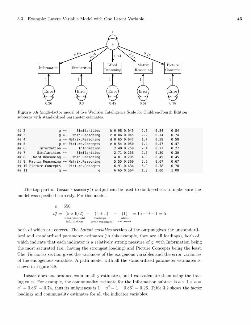
3.3. Example: Latent Variable Model with One Latent Variable 45
g
WordReasoningSimilaritiesInformation
MatrixReasoning
PictureConcepts
Error Error Error Error Error
0.86 0.84 0.74
0.580.47
1 1 1 1 1
0.26 0.3 0.45 0.67 0.78
1
Figure 3.8 Single-factor model of five Wechsler Intelligence Scale for Children-Fourth Editionsubtests with standardized parameter estimates.
## 2 g =~ Similarities b 0.98 0.045 2.5 0.84 0.84## 3 g =~ Word.Reasoning c 0.86 0.045 2.2 0.74 0.74## 4 g =~ Matrix.Reasoning d 0.65 0.047 1.7 0.58 0.58## 5 g =~ Picture.Concepts e 0.54 0.050 1.4 0.47 0.47## 6 Information ~~ Information 2.40 0.250 2.4 0.27 0.27## 7 Similarities ~~ Similarities 2.71 0.258 2.7 0.30 0.30## 8 Word.Reasoning ~~ Word.Reasoning 4.01 0.295 4.0 0.45 0.45## 9 Matrix.Reasoning ~~ Matrix.Reasoning 5.55 0.360 5.6 0.67 0.67## 10 Picture.Concepts ~~ Picture.Concepts 6.91 0.434 6.9 0.78 0.78## 11 g ~~ g 6.65 0.564 1.0 1.00 1.00
The top part of lavaan’s summary() output can be used to double-check to make sure themodel was specified correctly. For this model:
n = 550df = (5× 6/2)
non-redundantinformation
− (4 + 5)loadings +
error varainces
− (1)latent
variances
= 15− 9− 1 = 5
both of which are correct. The Latent variables section of the output gives the unstandard-ized and standardized parameter estimates (in this example, they are all loadings), both ofwhich indicate that each indicator is a relatively strong measure of g, with Information beingthe most saturated (i.e., having the strongest loading) and Picture Concepts being the least.The Variances section gives the variances of the exogenous variables and the error variancesof the endogenous variables. A path model with all the standardized parameter estimates isshown in Figure 3.8.
lavaan does not produce communality estimates, but I can calculate them using the trac-ing rules. For example, the communality estimate for the Information subtest is a× 1× a =a
2 = 0.862 = 0.74, thus its uniqueness is 1− a2 = 1− 0.862 = 0.26. Table 3.2 shows the factorloadings and communality estimates for all the indicator variables.
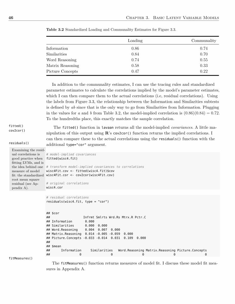
46 Chapter 3. Basic Latent Variable Models
Table 3.2 Standardized Loading and Communality Estimates for Figure 3.3.
Loading Communality
Information 0.86 0.74Similarities 0.84 0.70Word Reasoning 0.74 0.55Matrix Reasoning 0.58 0.33Picture Concepts 0.47 0.22
fitted()
cov2cor()
residuals()
Examining the resid-ual correlations isgood practice whenfitting LVMs, and isthe idea behind onemeasure of modelfit: the standardizedroot mean squareresidual (see Ap-pendix A).
fitMeasures()
In addition to the communality estimates, I can use the tracing rules and standardizedparameter estimates to calculate the correlations implied by the model’s parameter estimates,which I can then compare them to the actual correlations (i.e, residual correlations). Usingthe labels from Figure 3.3, the relationship between the Information and Similarities subtestsis defined by ab since that is the only way to go from Similarities from Information. Pluggingin the values for a and b from Table 3.2, the model-implied correlation is (0.86)(0.84) = 0.72.To the hundredths place, this exactly matches the sample correlation.
The fitted() function in lavaan returns all the model-implied covariances. A little ma-nipulation of this output using R’s cov2cor() function returns the implied correlations. Ican then compare these to the actual correlations using the residuals() function with theadditional type="cor" argument.
# model-implied covariancesfitted(wisc4.fit)
# transform model-implied covariances to correlationswisc4Fit.cov <- fitted(wisc4.fit)$covwisc4Fit.cor <- cov2cor(wisc4Fit.cov)
# original correlationswisc4.cor
# residual correlationsresiduals(wisc4.fit, type = "cor")
## $cor## Infrmt Smlrts Wrd.Rs Mtrx.R Pctr.C## Information 0.000## Similarities 0.000 0.000## Word.Reasoning 0.004 0.007 0.000## Matrix.Reasoning 0.014 -0.005 -0.059 0.000## Picture.Concepts -0.033 -0.014 0.031 0.109 0.000#### $mean## Information Similarities Word.Reasoning Matrix.Reasoning Picture.Concepts## 0 0 0 0 0
The fitMeasures() function returns measures of model fit. I discuss these model fit mea-sures in Appendix A.
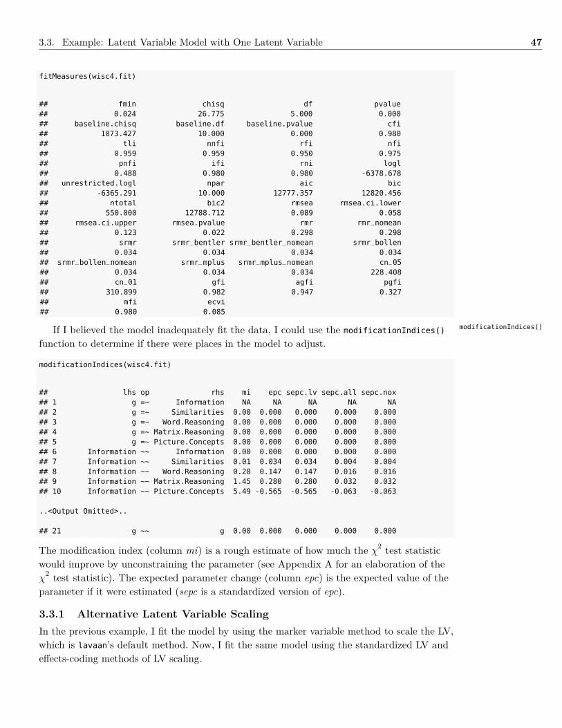
3.3. Example: Latent Variable Model with One Latent Variable 47
fitMeasures(wisc4.fit)
## fmin chisq df pvalue## 0.024 26.775 5.000 0.000## baseline.chisq baseline.df baseline.pvalue cfi## 1073.427 10.000 0.000 0.980## tli nnfi rfi nfi## 0.959 0.959 0.950 0.975## pnfi ifi rni logl## 0.488 0.980 0.980 -6378.678## unrestricted.logl npar aic bic## -6365.291 10.000 12777.357 12820.456## ntotal bic2 rmsea rmsea.ci.lower## 550.000 12788.712 0.089 0.058## rmsea.ci.upper rmsea.pvalue rmr rmr_nomean## 0.123 0.022 0.298 0.298## srmr srmr_bentler srmr_bentler_nomean srmr_bollen## 0.034 0.034 0.034 0.034## srmr_bollen_nomean srmr_mplus srmr_mplus_nomean cn_05## 0.034 0.034 0.034 228.408## cn_01 gfi agfi pgfi## 310.899 0.982 0.947 0.327## mfi ecvi## 0.980 0.085
If I believed the model inadequately fit the data, I could use the modificationIndices()
function to determine if there were places in the model to adjust.
modificationIndices(wisc4.fit)
## lhs op rhs mi epc sepc.lv sepc.all sepc.nox## 1 g =~ Information NA NA NA NA NA## 2 g =~ Similarities 0.00 0.000 0.000 0.000 0.000## 3 g =~ Word.Reasoning 0.00 0.000 0.000 0.000 0.000## 4 g =~ Matrix.Reasoning 0.00 0.000 0.000 0.000 0.000## 5 g =~ Picture.Concepts 0.00 0.000 0.000 0.000 0.000## 6 Information ~~ Information 0.00 0.000 0.000 0.000 0.000## 7 Information ~~ Similarities 0.01 0.034 0.034 0.004 0.004## 8 Information ~~ Word.Reasoning 0.28 0.147 0.147 0.016 0.016## 9 Information ~~ Matrix.Reasoning 1.45 0.280 0.280 0.032 0.032## 10 Information ~~ Picture.Concepts 5.49 -0.565 -0.565 -0.063 -0.063
..<Output Omitted>..
## 21 g ~~ g 0.00 0.000 0.000 0.000 0.000
The modification index (column mi) is a rough estimate of how much the χ2 test statisticwould improve by unconstraining the parameter (see Appendix A for an elaboration of theχ
2 test statistic). The expected parameter change (column epc) is the expected value of theparameter if it were estimated (sepc is a standardized version of epc).
3.3.1 Alternative Latent Variable ScalingIn the previous example, I fit the model by using the marker variable method to scale the LV,which is lavaan’s default method. Now, I fit the same model using the standardized LV andeffects-coding methods of LV scaling.
modificationIndices()
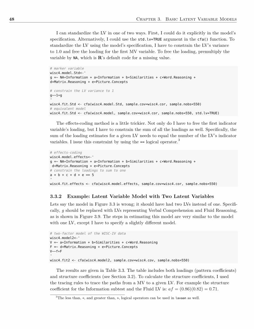
48 Chapter 3. Basic Latent Variable Models
I can standardize the LV in one of two ways. First, I could do it explicitly in the model’sspecification. Alternatively, I could use the std.lv=TRUE argument in the cfa() function. Tostandardize the LV using the model’s specification, I have to constrain the LV’s varianceto 1.0 and free the loading for the first MV variable. To free the loading, premultiply thevariable by NA, which is R’s default code for a missing value.
# marker variablewisc4.model.Std<-'g =~ NA*Information + a*Information + b*Similarities + c*Word.Reasoning +d*Matrix.Reasoning + e*Picture.Concepts
# constrain the LV variance to 1g~~1*g'wisc4.fit.Std <- cfa(wisc4.model.Std, sample.cov=wisc4.cor, sample.nobs=550)# equivalent modelwisc4.fit.Std <- cfa(wisc4.model, sample.cov=wisc4.cor, sample.nobs=550, std.lv=TRUE)
The effects-coding method is a little trickier. Not only do I have to free the first indicatorvariable’s loading, but I have to constrain the sum of all the loadings as well. Specifically, thesum of the loading estimates for a given LV needs to equal the number of the LV’s indicatorvariables. I issue this constraint by using the == logical operator.3
# effects-codingwisc4.model.effects<-'g =~ NA*Information + a*Information + b*Similarities + c*Word.Reasoning +d*Matrix.Reasoning + e*Picture.Concepts
# constrain the loadings to sum to onea + b + c + d + e == 5'wisc4.fit.effects <- cfa(wisc4.model.effects, sample.cov=wisc4.cor, sample.nobs=550)
3.3.2 Example: Latent Variable Model with Two Latent VariablesLets say the model in Figure 3.3 is wrong; it should have had two LVs instead of one. Specifi-cally, g should be replaced with LVs representing Verbal Comprehension and Fluid Reasoning,as is shown in Figure 3.9. The steps in estimating this model are very similar to the modelwith one LV, except I have to specify a slightly different model.
# two-factor model of the WISC-IV datawisc4.model2<-'V =~ a*Information + b*Similarities + c*Word.ReasoningF =~ d*Matrix.Reasoning + e*Picture.ConceptsV~~f*F'wisc4.fit2 <- cfa(wisc4.model2, sample.cov=wisc4.cov, sample.nobs=550)
The results are given in Table 3.3. The table includes both loadings (pattern coefficients)and structure coefficients (see Section 3.2). To calculate the structure coefficients, I usedthe tracing rules to trace the paths from a MV to a given LV. For example the structurecoefficient for the Information subtest and the Fluid LV is: af = (0.86)(0.82) = 0.71.
3The less than, <, and greater than, >, logical operators can be used in lavaan as well.
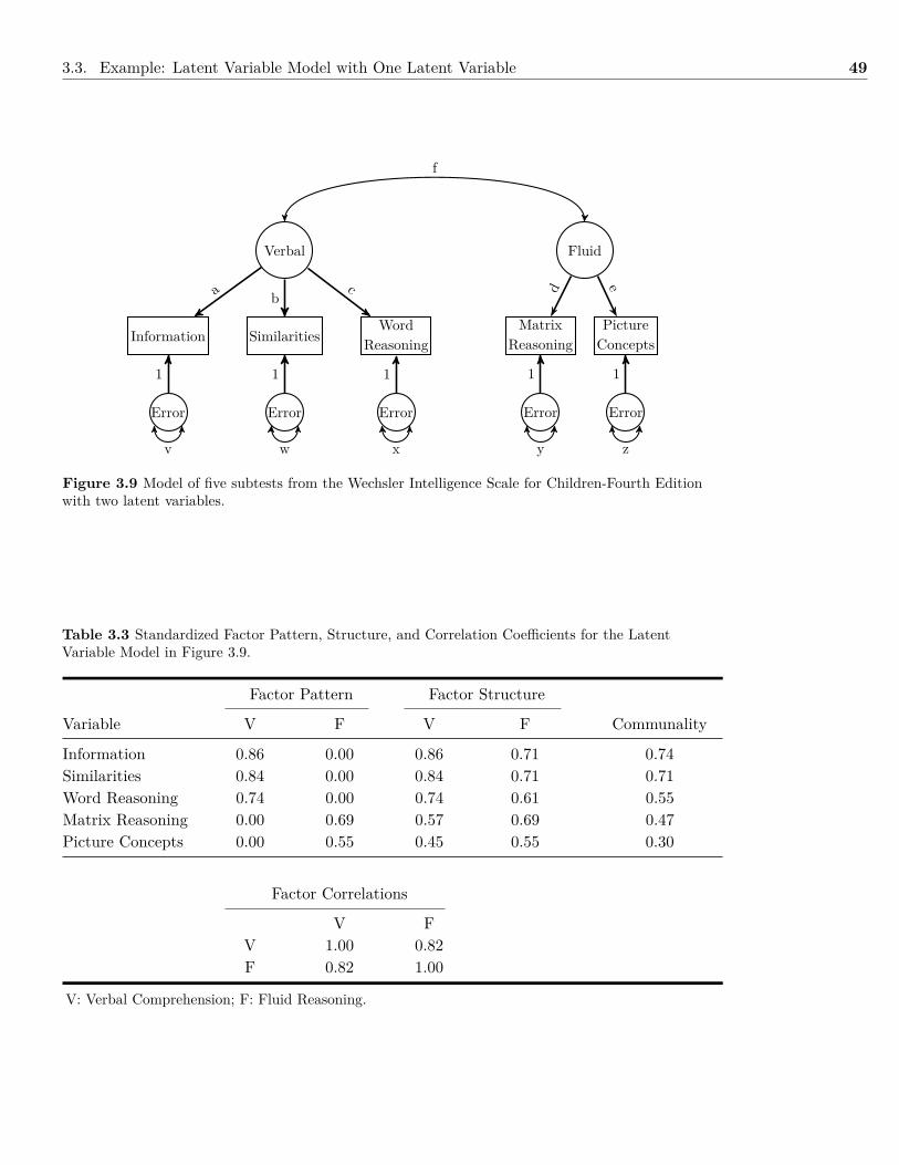
3.3. Example: Latent Variable Model with One Latent Variable 49
Verbal Fluid
SimilaritiesWord
ReasoningInformationMatrix
ReasoningPictureConcepts
Error Error Error Error Error
a bc d e
1 1 1 1 1
v w x y z
f
Figure 3.9 Model of five subtests from the Wechsler Intelligence Scale for Children-Fourth Editionwith two latent variables.
Table 3.3 Standardized Factor Pattern, Structure, and Correlation Coefficients for the LatentVariable Model in Figure 3.9.
Factor Pattern Factor Structure
Variable V F V F Communality
Information 0.86 0.00 0.86 0.71 0.74Similarities 0.84 0.00 0.84 0.71 0.71Word Reasoning 0.74 0.00 0.74 0.61 0.55Matrix Reasoning 0.00 0.69 0.57 0.69 0.47Picture Concepts 0.00 0.55 0.45 0.55 0.30
Factor Correlations
V FV 1.00 0.82F 0.82 1.00
V: Verbal Comprehension; F: Fluid Reasoning.
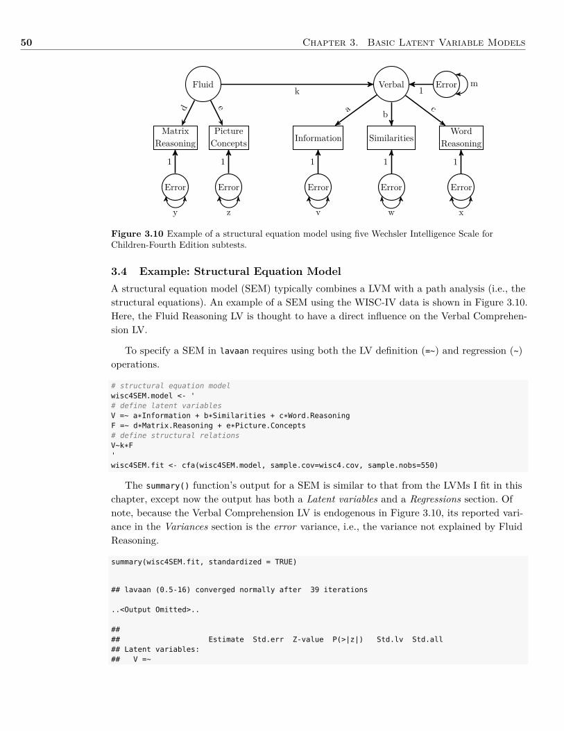
50 Chapter 3. Basic Latent Variable Models
Fluid Verbal
SimilaritiesWord
ReasoningInformationMatrix
ReasoningPictureConcepts
Error Error ErrorError Error
Error
a bcd e
1
1 1 11 1
v w xy z
mk
Figure 3.10 Example of a structural equation model using five Wechsler Intelligence Scale forChildren-Fourth Edition subtests.
3.4 Example: Structural Equation ModelA structural equation model (SEM) typically combines a LVM with a path analysis (i.e., thestructural equations). An example of a SEM using the WISC-IV data is shown in Figure 3.10.Here, the Fluid Reasoning LV is thought to have a direct influence on the Verbal Comprehen-sion LV.
To specify a SEM in lavaan requires using both the LV definition (=~) and regression (~)operations.
# structural equation modelwisc4SEM.model <- '# define latent variablesV =~ a*Information + b*Similarities + c*Word.ReasoningF =~ d*Matrix.Reasoning + e*Picture.Concepts# define structural relationsV~k*F'wisc4SEM.fit <- cfa(wisc4SEM.model, sample.cov=wisc4.cov, sample.nobs=550)
The summary() function’s output for a SEM is similar to that from the LVMs I fit in thischapter, except now the output has both a Latent variables and a Regressions section. Ofnote, because the Verbal Comprehension LV is endogenous in Figure 3.10, its reported vari-ance in the Variances section is the error variance, i.e., the variance not explained by FluidReasoning.
summary(wisc4SEM.fit, standardized = TRUE)
## lavaan (0.5-16) converged normally after 39 iterations
..<Output Omitted>..
#### Estimate Std.err Z-value P(>|z|) Std.lv Std.all## Latent variables:## V =~
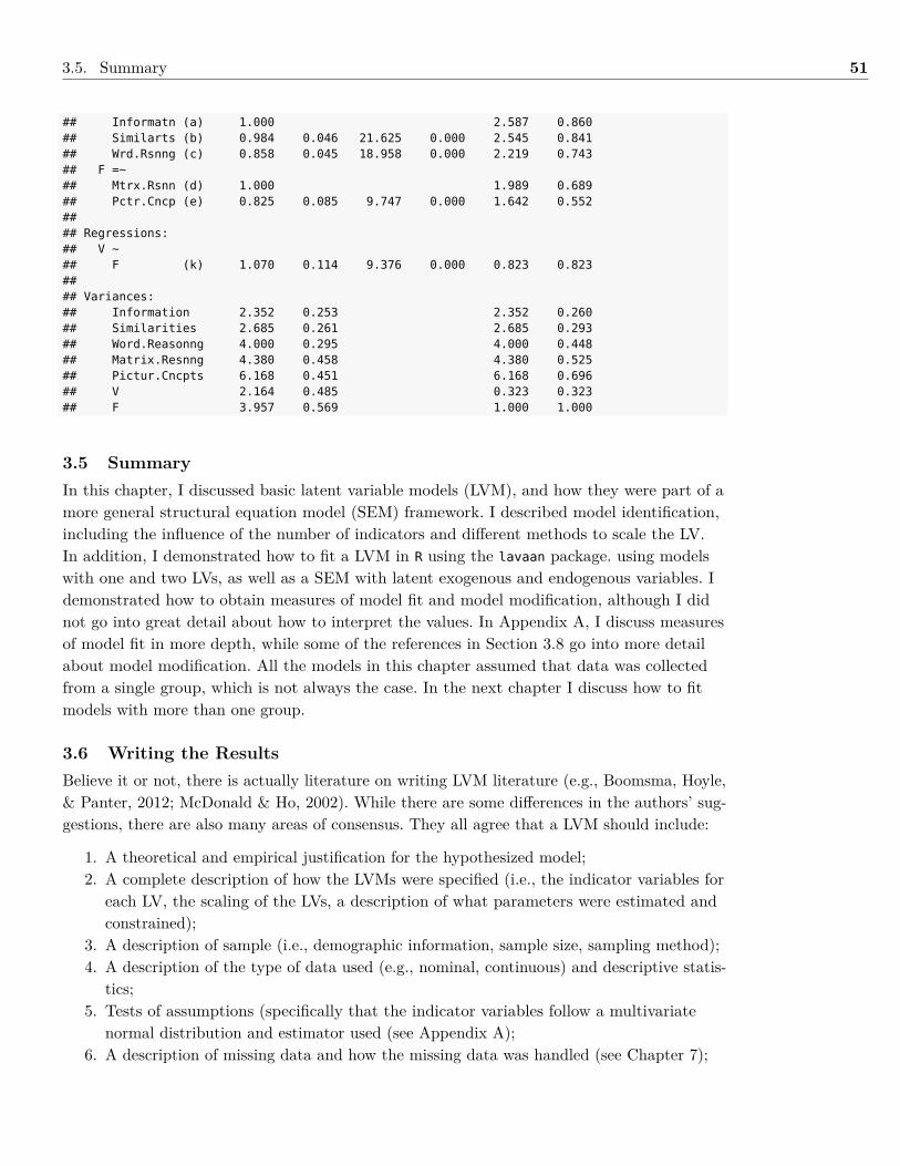
3.5. Summary 51
## Informatn (a) 1.000 2.587 0.860## Similarts (b) 0.984 0.046 21.625 0.000 2.545 0.841## Wrd.Rsnng (c) 0.858 0.045 18.958 0.000 2.219 0.743## F =~## Mtrx.Rsnn (d) 1.000 1.989 0.689## Pctr.Cncp (e) 0.825 0.085 9.747 0.000 1.642 0.552#### Regressions:## V ~## F (k) 1.070 0.114 9.376 0.000 0.823 0.823#### Variances:## Information 2.352 0.253 2.352 0.260## Similarities 2.685 0.261 2.685 0.293## Word.Reasonng 4.000 0.295 4.000 0.448## Matrix.Resnng 4.380 0.458 4.380 0.525## Pictur.Cncpts 6.168 0.451 6.168 0.696## V 2.164 0.485 0.323 0.323## F 3.957 0.569 1.000 1.000
3.5 SummaryIn this chapter, I discussed basic latent variable models (LVM), and how they were part of amore general structural equation model (SEM) framework. I described model identification,including the influence of the number of indicators and different methods to scale the LV.In addition, I demonstrated how to fit a LVM in R using the lavaan package. using modelswith one and two LVs, as well as a SEM with latent exogenous and endogenous variables. Idemonstrated how to obtain measures of model fit and model modification, although I didnot go into great detail about how to interpret the values. In Appendix A, I discuss measuresof model fit in more depth, while some of the references in Section 3.8 go into more detailabout model modification. All the models in this chapter assumed that data was collectedfrom a single group, which is not always the case. In the next chapter I discuss how to fitmodels with more than one group.
3.6 Writing the ResultsBelieve it or not, there is actually literature on writing LVM literature (e.g., Boomsma, Hoyle,& Panter, 2012; McDonald & Ho, 2002). While there are some differences in the authors’ sug-gestions, there are also many areas of consensus. They all agree that a LVM should include:
1. A theoretical and empirical justification for the hypothesized model;2. A complete description of how the LVMs were specified (i.e., the indicator variables for
each LV, the scaling of the LVs, a description of what parameters were estimated andconstrained);
3. A description of sample (i.e., demographic information, sample size, sampling method);4. A description of the type of data used (e.g., nominal, continuous) and descriptive statis-
tics;5. Tests of assumptions (specifically that the indicator variables follow a multivariate
normal distribution and estimator used (see Appendix A);6. A description of missing data and how the missing data was handled (see Chapter 7);
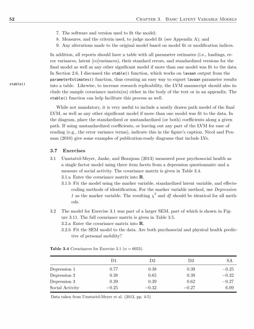
52 Chapter 3. Basic Latent Variable Models
xtable()
7. The software and version used to fit the model;8. Measures, and the criteria used, to judge model fit (see Appendix A); and9. Any alterations made to the original model based on model fit or modification indices.
In addition, all reports should have a table with all parameter estimates (i.e., loadings, er-ror variances, latent [co]variances), their standard errors, and standardized versions for thefinal model as well as any other significant model if more than one model was fit to the data.In Section 2.6, I discussed the xtable() function, which works on lavaan output from theparameterEstimates() function, thus creating an easy way to export lavaan parameter resultsinto a table. Likewise, to increase research replicability, the LVM manuscript should also in-clude the sample covariance matrix(es) either in the body of the text or in an appendix. Thextable() function can help facilitate this process as well.
While not mandatory, it is very useful to include a neatly drawn path model of the finalLVM, as well as any other significant model if more than one model was fit to the data. Inthe diagram, place the standardized or unstandardized (or both) coefficients along a givenpath. If using unstandardized coefficients, or leaving out any part of the LVM for ease ofreading (e.g., the error variance terms), indicate this in the figure’s caption. Nicol and Pex-man (2010) give some examples of publication-ready diagrams that include LVs.
3.7 Exercises3.1 Umstattd-Meyer, Janke, and Beaujean (2013) measured poor psychosocial health as
a single factor model using three item facets from a depression questionnaire and ameasure of social activity. The covariance matrix is given in Table 3.4.3.1.a Enter the covariance matrix into R.3.1.b Fit the model using the marker variable, standardized latent variable, and effects-
coding methods of identification. For the marker variable method, use Depression1 as the marker variable. The resulting χ2 and df should be identical for all meth-ods.
3.2 The model for Exercise 3.1 was part of a larger SEM, part of which is shown in Fig-ure 3.11. The full covariance matrix is given in Table 3.5.3.2.a Enter the covariance matrix into R.3.2.b Fit the SEM model to the data. Are both psychosocial and physical health predic-
tive of personal mobility?
Table 3.4 Covariances for Exercise 3.1 (n = 6053).
D1 D2 D3 SA
Depression 1 0.77 0.38 0.39 −0.25Depression 2 0.38 0.65 0.39 −0.32Depression 3 0.39 0.39 0.62 −0.27Social Activity −0.25 −0.32 −0.27 6.09
Data taken from Umstattd-Meyer et al. (2013, pp. 4-5)
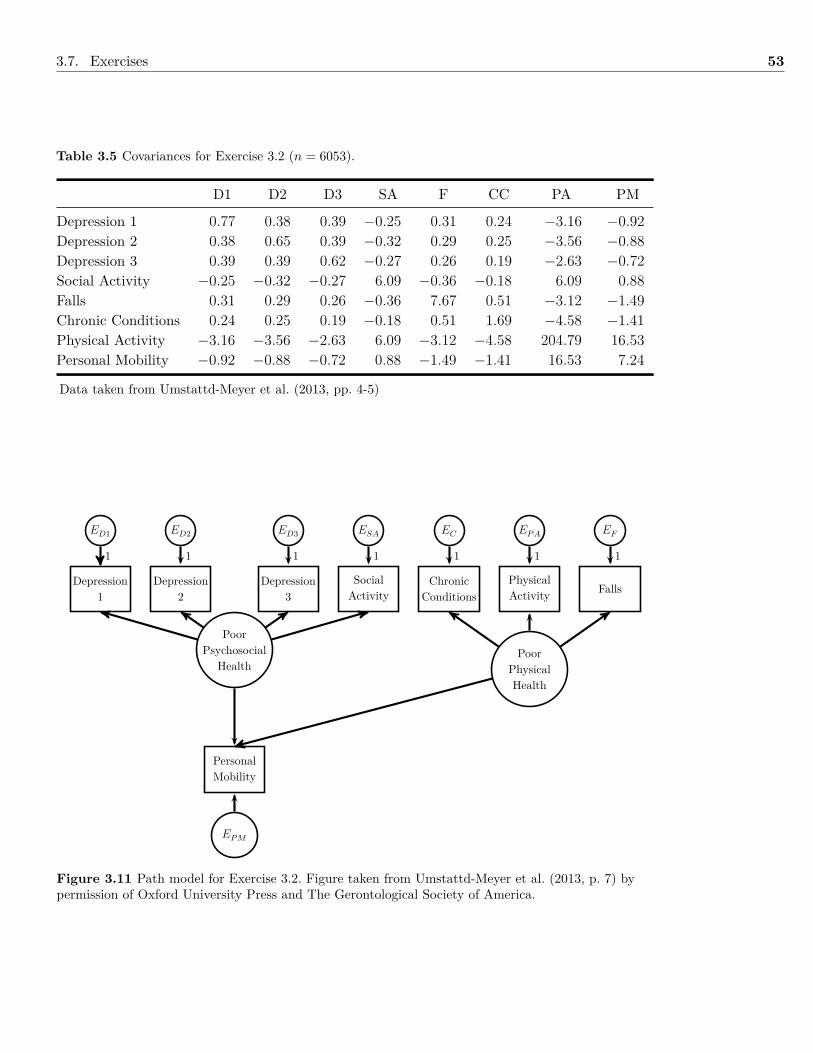
3.7. Exercises 53
Table 3.5 Covariances for Exercise 3.2 (n = 6053).
D1 D2 D3 SA F CC PA PM
Depression 1 0.77 0.38 0.39 −0.25 0.31 0.24 −3.16 −0.92Depression 2 0.38 0.65 0.39 −0.32 0.29 0.25 −3.56 −0.88Depression 3 0.39 0.39 0.62 −0.27 0.26 0.19 −2.63 −0.72Social Activity −0.25 −0.32 −0.27 6.09 −0.36 −0.18 6.09 0.88Falls 0.31 0.29 0.26 −0.36 7.67 0.51 −3.12 −1.49Chronic Conditions 0.24 0.25 0.19 −0.18 0.51 1.69 −4.58 −1.41Physical Activity −3.16 −3.56 −2.63 6.09 −3.12 −4.58 204.79 16.53Personal Mobility −0.92 −0.88 −0.72 0.88 −1.49 −1.41 16.53 7.24
Data taken from Umstattd-Meyer et al. (2013, pp. 4-5)
Depression1
Depression2
Depression3
SocialActivity
PoorPsychosocial
Health
ChronicConditions
PhysicalActivity Falls
PoorPhysicalHealth
ED1 ED2 ED3 ESA EC EPA EF
PersonalMobility
EPM
1 1 1 1 1 1 1
Figure 3.11 Path model for Exercise 3.2. Figure taken from Umstattd-Meyer et al. (2013, p. 7) bypermission of Oxford University Press and The Gerontological Society of America.
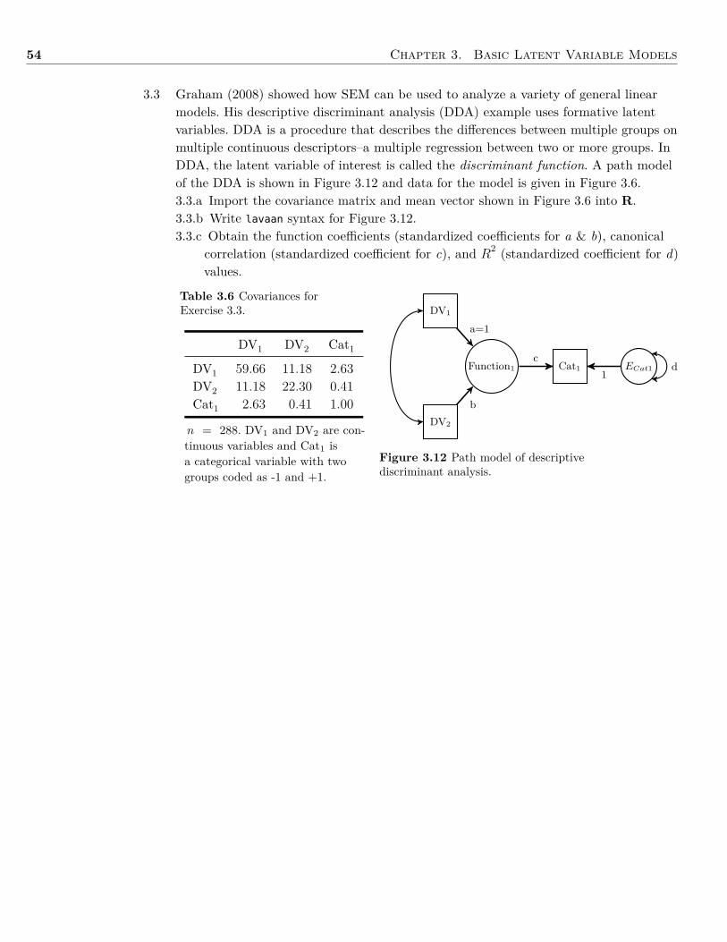
54 Chapter 3. Basic Latent Variable Models
3.3 Graham (2008) showed how SEM can be used to analyze a variety of general linearmodels. His descriptive discriminant analysis (DDA) example uses formative latentvariables. DDA is a procedure that describes the differences between multiple groups onmultiple continuous descriptors–a multiple regression between two or more groups. InDDA, the latent variable of interest is called the discriminant function. A path modelof the DDA is shown in Figure 3.12 and data for the model is given in Figure 3.6.3.3.a Import the covariance matrix and mean vector shown in Figure 3.6 into R.3.3.b Write lavaan syntax for Figure 3.12.3.3.c Obtain the function coefficients (standardized coefficients for a & b), canonical
correlation (standardized coefficient for c), and R2 (standardized coefficient for d)values.
Table 3.6 Covariances forExercise 3.3.
DV1 DV2 Cat1
DV1 59.66 11.18 2.63DV2 11.18 22.30 0.41Cat1 2.63 0.41 1.00
n = 288. DV1 and DV2 are con-tinuous variables and Cat1 isa categorical variable with twogroups coded as -1 and +1.
Function1
DV1
DV2
Cat1 ECat1
a=1
b
c1
d
Figure 3.12 Path model of descriptivediscriminant analysis.
3.8. References & Further Readings 55
3.8 References & Further ReadingsBeaujean, A. A. (2013). Factor analysis using R. Practical Assessment, Research, and
Evaluation, 18 (4), 1-11. Retrieved from http://pareonline.net/pdf/v18n4.pdf.Bollen, K. A. (2002). Latent variables in psychology and the social sciences. Annual Review of
Psychology, 53 , 605-634. doi: 10.1146/annurev.psych.53.100901.135239Boomsma, A., Hoyle, R. H., & Panter, A. T. (2012). The structural equation modeling
research report. In R. H. Hoyle (Ed.), Handbook of structural equation modeling. NewYork, NY: Guilford.
Brown, T. A. (2006). Confirmatory factor analysis for applied research. New York, NY:Guilford Press.
Chou, C.-p., & Huh, J. (2012). Model modification in structural equation modeling. InR. A. Hoyle (Ed.), Handbook of structural equation modeling (pp. 232–246). New York,NY: Guilford.
Edwards, J. R., & Bagozzi, R. P. (2000). On the nature and direction of relationships betweenconstructs and measures. Psychological Methods, 5 , 155-174. doi:10.1037/1082-989X.5.2.155
Graham, J. M. (2008). The general linear model as structural equation modeling. Journal ofEducational and Behavioral Statistics, 33 , 485-506. doi: 10.3102/1076998607306151
Kenny, D. A., Kashy, D., & Bolger, N. (1988). Data analysis in social psychology. InD. Gilbert, S. Fiske, & G. Lindzey (Eds.), Handbook of social psychology (4th ed., pp.233–265). New York, NY: McGraw-Hill.
Little, T. D., Slegers, D. W., & Card, N. A. (2006). A non-arbitrary method of identifying andscaling latent variables in SEM and MACS models. Structural Equation Modeling: AMultidisciplinary Journal, 13 , 59-72. doi: 10.1207/s15328007sem1301_3
Loehlin, J. C. (2004). Latent variable models: An introduction to factor, path, and structuralequation analysis (4th ed.). Mahwah, NJ: Erlbaum.
McDonald, R. P., & Ho, M.-H. R. (2002). Principles and practice in reporting structuralequation analyses. Psychological Methods, 7 , 64-82. doi: 10.1037/1082-989X.7.1.64
Nicol, A. A. M., & Pexman, P. M. (2010). Displaying your findings: A practical guide forcreating figures, posters, and presentations (6th ed.). Washington, DC: AmericanPsychological Association.
Parkin, J., & Beaujean, A. A. (2012). The effects of Wechsler Intelligence Scale forChildren-Fourth Edition cognitive abilities on math achievement. Journal of SchoolPsychology, 50 , 113-128. doi: 10.1016/j.jsp.2011.08.003
Umstattd-Meyer, M. R., Janke, M. C., & Beaujean, A. A. (2013). Predictors of older adults’personal and community mobility: Using a comprehensive theoretical mobilityframework. The Gerontologist, Advance online publication. doi: 10.1093/geront/gnt054
Wechsler, D. (2003). Wechsler intelligence scale for children (4th ed.). San Antonio, TX: ThePsychological Corporation.
Mean andCovarianceStructure(MACS)
4 | Latent Variable Models withMultiple Groups
Chapter Contents4.1 Background . . . . . . . . . . . . . . . . . . . . . . . . . . . . . . . . . . . . 564.2 Invariance . . . . . . . . . . . . . . . . . . . . . . . . . . . . . . . . . . . . . 56
4.2.1 Means and Intercepts . . . . . . . . . . . . . . . . . . . . . . . . . . . 574.2.2 Types of Measurement Invariance . . . . . . . . . . . . . . . . . . . . 584.2.3 Evaluating Invariance . . . . . . . . . . . . . . . . . . . . . . . . . . 61
4.3 Group Equality Constraints . . . . . . . . . . . . . . . . . . . . . . . . . . . 614.4 Example: Invariance . . . . . . . . . . . . . . . . . . . . . . . . . . . . . . . . 624.5 Using Labels for Parameter Constraints . . . . . . . . . . . . . . . . . . . . . 704.6 Example: Genetically Informative Design . . . . . . . . . . . . . . . . . . . . 714.7 Summary . . . . . . . . . . . . . . . . . . . . . . . . . . . . . . . . . . . . . . 744.8 Writing the Results . . . . . . . . . . . . . . . . . . . . . . . . . . . . . . . . 754.9 Exercises . . . . . . . . . . . . . . . . . . . . . . . . . . . . . . . . . . . . . . 754.10 References & Further Readings . . . . . . . . . . . . . . . . . . . . . . . . . . 78
4.1 BackgroundThere are typically two reasons to include multiple groups in a LVM model. The first reasonis to examine if the LVM works the same across the groups. The second reason is when theestimation of certain parameters require data from two or more unique groups, as is donewith genetically informative designs.
4.2 InvarianceThe general question of invariance is one of whether or not, under different condi-tions of observing and studying phenomena, measurements yield measures of thesame attributes. If there is no evidence indicating presence or absence of measure-ment invariance-the usual case-or there is evidence that such invariance does notobtain, then the basis for drawing scientific inference is severely lacking: findingsof differences between individuals and groups cannot be unambiguously interpreted.(Horn & McArdle, 1992, p. 117, emphasis added)
A question that often arises when examining group differences on a variable is if any ob-served differences are due to differences in the groups themselves or differences in the in-strument(s) used to measure the variable. One of the more useful ways of answering thisquestion is by assessing invariance in LVs. To do so, however, requires I adjust the LVM Iintroduced in Chapter 3 to include both covariances and means, which is why these modelsare sometimes referred to as mean and covariance structure (MACS) models. A MACSpath model is shown in Figure 4.1.
56
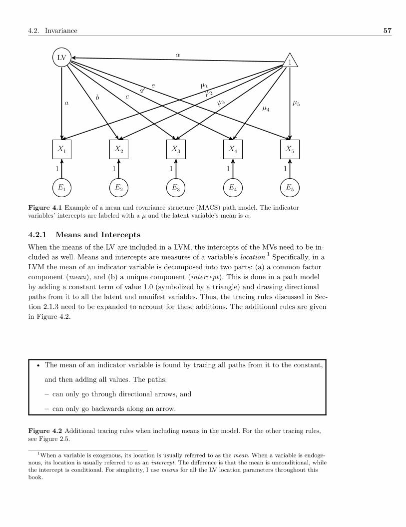
4.2. Invariance 57
X3X2X1 X4 X5
E1 E2 E3 E4 E5
LV 1
ab c
de
1 1 1 1 1
µ1µ2
µ 3µ4
µ5
α
Figure 4.1 Example of a mean and covariance structure (MACS) path model. The indicatorvariables’ intercepts are labeled with a µ and the latent variable’s mean is α.
4.2.1 Means and InterceptsWhen the means of the LV are included in a LVM, the intercepts of the MVs need to be in-cluded as well. Means and intercepts are measures of a variable’s location.1 Specifically, in aLVM the mean of an indicator variable is decomposed into two parts: (a) a common factorcomponent (mean), and (b) a unique component (intercept). This is done in a path modelby adding a constant term of value 1.0 (symbolized by a triangle) and drawing directionalpaths from it to all the latent and manifest variables. Thus, the tracing rules discussed in Sec-tion 2.1.3 need to be expanded to account for these additions. The additional rules are givenin Figure 4.2.
• The mean of an indicator variable is found by tracing all paths from it to the constant,
and then adding all values. The paths:
– can only go through directional arrows, and
– can only go backwards along an arrow.
Figure 4.2 Additional tracing rules when including means in the model. For the other tracing rules,see Figure 2.5.
1When a variable is exogenous, its location is usually referred to as the mean. When a variable is endoge-nous, its location is usually referred to as an intercept. The difference is that the mean is unconditional, whilethe intercept is conditional. For simplicity, I use means for all the LV location parameters throughout thisbook.
58 Chapter 4. Latent Variable Models with Multiple Groups
MeasurementInvariance
ConfiguralInvariance
As an example, in Figure 4.1 the path for the mean of the manifest variable X1, x̄1, is
a× α + µ1 = x̄
The a× α path is the common factor component (i.e., mean) and µ1 path is the unique compo-nent (i.e., intercept).
4.2.1.1 Identification with Means and Intercepts in the ModelWhen means and intercepts are included in a path model, each MV’s observed mean needsto be included in the input. The formula to calculate the number of non-redundant pieces ofinformation in a dataset with means is given in Equation (4.1).
non-redundant information in a dataset with means = p(p+ 1)2 +m = p(p+ 3)
2 (4.1)
where p is the number of manifest variables.
For MACS models to be identified, all the free location (means/intercepts) and scale (vari-ances) parameters have to be estimated uniquely. Thus, I need to add to the identificationrules-of-thumb I presented in Section 3.2.1 to account for means and intercepts. There arethree ways to do this that map onto one of the three methods of LV scaling I presented inSection 3.2.1.2.
1. Standardized latent variable. For this method, in addition to fixing the latent varianceto 1.0 (to fix the LV’s scales), it also requires fixing the latent means to 0.0 (to fix theLV’s location). This allows the estimation of all the indicator variables’ intercepts, al-though they will be equal to the indicator variables’ means.
2. Marker variable. For this method, the LV’s scale is set by fixing one indicator variable’sloading to 1.0 for each LV. To set the LV’s mean, the same indicator variable’s inter-cepts is fixed to 0.0. This sets the LVs to have scales and locations directly related tothe marker variable.
3. Effects-coding. To set a LV’s scale with this method, the loadings of its indicator vari-ables need to be constrained to sum to the number of its indicators. To set the LV’slocation, constrain the intercepts of a LV’s indicator variables to sum to 0.0. Thismethod forces the mean and variance of the LV to be the weighted average of all ofits indicator variables’ means and loadings.
4.2.2 Types of Measurement InvarianceMeasurement invariance is not an all-or-nothing concept. Instead, there are degrees ofinvariance, usually described as a hierarchical sequence starting with the weakest form andworking up to the strictest form. I describe the different levels of invariance below as well aspresent them in Table 4.1.
1. Configural. This is the most basic level, and just indicates that LVMs have the samestructure in all the groups. That is, the groups have the same number of LVs, formedby the same number of indicator variables, all of which have the same pattern of con-strained and estimated parameters. There is no requirement that any estimated coeffi-
4.2. Invariance 59
cients are equal across groups, but the price for these weak assumptions is that thereis no reason to believe that the LVs are measuring the same construct in each group.Thus, this level of invariance does not warrant any between-group comparisons of theconstructs the LVs represent.
2. Weak. This level adds that, for a given indicator, the loadings are the same acrossgroups. Latent variances are allowed to vary among groups, though.2 With weak in-variance, there is a weak argument that the LVs are equivalent between groups, but, atmost, this condition only allows a comparison of the latent variances and covariances.
3. Strong. This level of invariance adds the constraint that, for a given indicator variable,the intercepts are the same among groups. When constraining the intercepts, the latentmeans are allowed to vary among groups. With this level of invariance, individuals atthe same level of a given LV have the same expected value on the indicator variables,irrespective of group membership. Moreover, strong invariance allows for comparisonsof the LV. Specifically, latent means, variances, and covariances can all be comparedamong groups. If there are group differences on strongly-invariant LVs, it likely indi-cates that there are real difference in these variables, as opposed to the difference beingin how the LVs are measured.
4. Strict. This level adds that, for a given indicator, the error variances are constrainedto be equal across groups. Usually this level of invariance is not required for makingcross-group comparisons of the LVs. Because the error terms in a LVM are comprisedof random error variance as well as indicator-specific variance, there is not necessarilythe expectation that they would be the same among the groups. Thus, this form ofinvariance is usually tested, in conjunction with evaluating invariance of the latent vari-ances (level 5), when the area of interest is the reliability of the construct the LV rep-resents. If the latent variances are invariant among the groups, then evaluating strictinvariance is really an investigation of construct reliability invariance.
5. Homogeneity of Latent Variable Variances. The variance of a LV represents itsdispersion, and thus represents how much variability there is in the construct that theLV represents varies within groups. If there is homogeneity of the latent variances, thisindicates the groups used equivalent ranges of the construct for the indicator variables’values. If this does not hold, however, this indicates that the group with the smalleramount of latent variance is using a narrower range of the construct than the groupwith the larger amount. Evaluating homogeneity of latent covarinaces can be done, too,but there is usually not much to be gained from such an analysis.
6. Homogeneity of Factor Means. This level of invariance indicates no differencesamong groups in the average level of the construct the LV represents. Like the moretraditional analyses of mean differences (e.g., ANOVA), if there is more than one groupthen the test of a latent variable’s mean differences usually begins with an omnibustest that constrains the means to be equal across all groups. If this model does not fitthe data well, then subsequent tests may be conducted to isolate specific group differ-ences.
Weak Invariance
Strong Invariance
Strict Invariance
2Since the latent variances are constrained to be the same at this level, weak invariance really just showsthat the loadings are only proportionally equivalent. This is akin to predicting weight from height in twogroups. In the first group, height is measured in feet, but in the second group it is measured in inches.
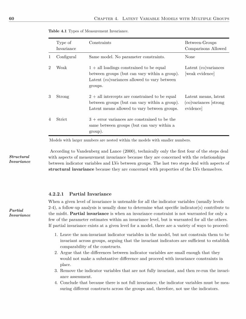
60 Chapter 4. Latent Variable Models with Multiple Groups
Table 4.1 Types of Measurement Invariance.
Type ofInvariance
Constraints Between-GroupsComparisons Allowed
1 Configural Same model. No parameter constraints. None
2 Weak 1 + all loadings constrained to be equalbetween groups (but can vary within a group).Latent (co)variances allowed to vary betweengroups.
Latent (co)variances[weak evidence]
3 Strong 2 + all intercepts are constrained to be equalbetween groups (but can vary within a group).Latent means allowed to vary between groups.
Latent means, latent(co)variances [strongevidence]
4 Strict 3 + error variances are constrained to be thesame between groups (but can vary within agroup).
Models with larger numbers are nested within the models with smaller numbers.
StructuralInvariance
PartialInvariance
According to Vandenberg and Lance (2000), technically only the first four of the steps dealwith aspects of measurement invariance because they are concerned with the relationshipsbetween indicator variables and LVs between groups. The last two steps deal with aspects ofstructural invariance because they are concerned with properties of the LVs themselves.
4.2.2.1 Partial InvarianceWhen a given level of invariance is untenable for all the indicator variables (usually levels2-4), a follow-up analysis is usually done to determine what specific indicator(s) contribute tothe misfit. Partial invariance is when an invariance constraint is not warranted for only afew of the parameter estimates within an invariance level, but is warranted for all the others.If partial invariance exists at a given level for a model, there are a variety of ways to proceed:
1. Leave the non-invariant indicator variables in the model, but not constrain them to beinvariant across groups, arguing that the invariant indicators are sufficient to establishcomparability of the constructs.
2. Argue that the differences between indicator variables are small enough that theywould not make a substantive difference and proceed with invariance constraints inplace.
3. Remove the indicator variables that are not fully invariant, and then re-run the invari-ance assessment.
4. Conclude that because there is not full invariance, the indicator variables must be mea-suring different constructs across the groups and, therefore, not use the indicators.
4.3. Group Equality Constraints 61
Usually, a mix of options 1 and 2 are used in practice, although 3 is useful in some circum-stances. Option 4 becomes the best alternative when the number of indicator variables notexhibiting invariance is too high.
4.2.3 Evaluating InvarianceBecause invariance involves a hierarchy of models, testing for invariance requires a multi-stepprocedure, testing more restrictive models at each step.3 As with assessing the fit of a modelfor a single group, there are multiple ways to examine if the increasingly restrictive modelsin Section 4.2.2 are consistent with the data. One approach is the statistical approach, whichexamines the change in χ2 values (∆χ2) across nested models (see Appendix A for more onnested models).4 If, as the models grow more restrictive, the ∆χ2 values do not significantlychange (i.e, the p-value for ∆χ2 is > some pre-set type 1 error level), this is taken as evi-dence that the more restrictive model (i.e., higher-level of invariance) fits data as well as theless restrictive model; thus, the more restrictive model should be favored over the less restric-tive one since it is more parsimonious (i.e,. estimates fewer parameters).
An alternative approach to evaluating invariance is to use a modeling approach. As withthe statistical approach, increasingly-constrained models are evaluated against each other,only this approach uses approximate fit indices (AFI) to determine what model to use (seeAppendix A for types of AFIs). For this approach, if a model with a given set of invarianceconstraints has an adequate level of fit on the AFIs, then the invariance constraints are rea-sonable additions to the LVM. The question you are probably asking is, What fit indices doI use for the modeling approach to evaluate invariance? Meade, Johnson, and Braddy (2008)did a Monte Carlo study (see Chapter 8 for more on Monte Carlo studies) and suggested thecomparative fit index (CFI) and McDonald’s noncentrality fit index (MFI) were relativelyrobust. Thus, the modeling approach would recommend that invariance be based on twocriteria:(a) the multi-group factor model with constraints exhibits an adequate fit to the dataaccording to the AFIs; and (b) the change in the CFI and MFI values from one model to amore restrictive (nested) model is negligible.
4.3 Group Equality ConstraintsBefore working through an invariance example in R, I briefly discuss general parameter con-straints in LVMs. For some LVMs, there is a need to constrain a parameter estimate to beequal to a specific value, to be greater/less than a specific value, or to be equal to another pa-rameter estimate (which includes the same parameter estimate across groups). There are twoways to constrain parameters in lavaan (and almost any other LV program). The first way toconstrain parameters is by using parameter labels, which I discuss in Section 4.5. The secondway is to use group equality constraints, which impose equality constraints on a whole set ofparameter estimates (e.g., all intercepts) among groups using the group.equal argument inthe cfa() or sem() functions. These take the general form of group.equal="m", where m is one
See Meade et al’s(2008) article formore informationon negligible valuechanges.
3The alternative would be to conduct omnibus tests for equality of the indicators’ covariances and meansamong the groups as the initial step. If that model fit the data well, then there would not be a need for anyfurther invariance investigation.
4The df for ∆χ2 are the difference between the nested models’ df.
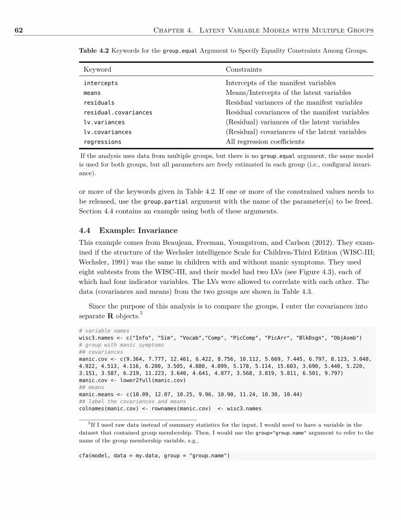
62 Chapter 4. Latent Variable Models with Multiple Groups
Table 4.2 Keywords for the group.equal Argument to Specify Equality Constraints Among Groups.
Keyword Constraints
intercepts Intercepts of the manifest variablesmeans Means/Intercepts of the latent variablesresiduals Residual variances of the manifest variablesresidual.covariances Residual covariances of the manifest variableslv.variances (Residual) variances of the latent variableslv.covariances (Residual) covariances of the latent variablesregressions All regression coefficients
If the analysis uses data from multiple groups, but there is no group.equal argument, the same modelis used for both groups, but all parameters are freely estimated in each group (i.e., configural invari-ance).
or more of the keywords given in Table 4.2. If one or more of the constrained values needs tobe released, use the group.partial argument with the name of the parameter(s) to be freed.Section 4.4 contains an example using both of these arguments.
4.4 Example: InvarianceThis example comes from Beaujean, Freeman, Youngstrom, and Carlson (2012). They exam-ined if the structure of the Wechsler intelligence Scale for Children-Third Edition (WISC-III;Wechsler, 1991) was the same in children with and without manic symptoms. They usedeight subtests from the WISC-III, and their model had two LVs (see Figure 4.3), each ofwhich had four indicator variables. The LVs were allowed to correlate with each other. Thedata (covariances and means) from the two groups are shown in Table 4.3.
Since the purpose of this analysis is to compare the groups, I enter the covariances intoseparate R objects.5
# variable nameswisc3.names <- c("Info", "Sim", "Vocab","Comp", "PicComp", "PicArr", "BlkDsgn", "ObjAsmb")# group with manic symptoms## covariancesmanic.cov <- c(9.364, 7.777, 12.461, 6.422, 8.756, 10.112, 5.669, 7.445, 6.797, 8.123, 3.048,4.922, 4.513, 4.116, 6.200, 3.505, 4.880, 4.899, 5.178, 5.114, 15.603, 3.690, 5.440, 5.220,3.151, 3.587, 6.219, 11.223, 3.640, 4.641, 4.877, 3.568, 3.819, 5.811, 6.501, 9.797)manic.cov <- lower2full(manic.cov)## meansmanic.means <- c(10.09, 12.07, 10.25, 9.96, 10.90, 11.24, 10.30, 10.44)## label the covariances and meanscolnames(manic.cov) <- rownames(manic.cov) <- wisc3.names
5If I used raw data instead of summary statistics for the input, I would need to have a variable in thedataset that contained group membership. Then, I would use the group="group.name" argument to refer to thename of the group membership variable, e.g.,
cfa(model, data = my.data, group = "group.name")
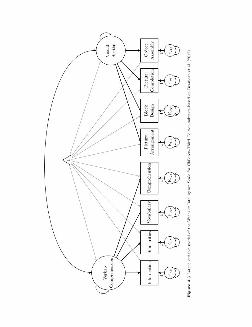
Verbal-
Com
prehen
sion
Inform
ation
Simila
rities
Vocabu
lary
Com
preh
ensio
nPicture
Arran
gement
Block
Design
Picture
Com
pletion
Object
Assem
bly
Visu
al-
Spatial
1
E IN
E SI
E VC
E CO
E PA
E BD
E PC
E OA
11
11
11
11
Figure4.3La
tent
varia
blemod
elof
theWechslerIntelligenceSc
aleforChildren-Third
Edition
subtests
basedon
Beaujeanet
al.(20
12).
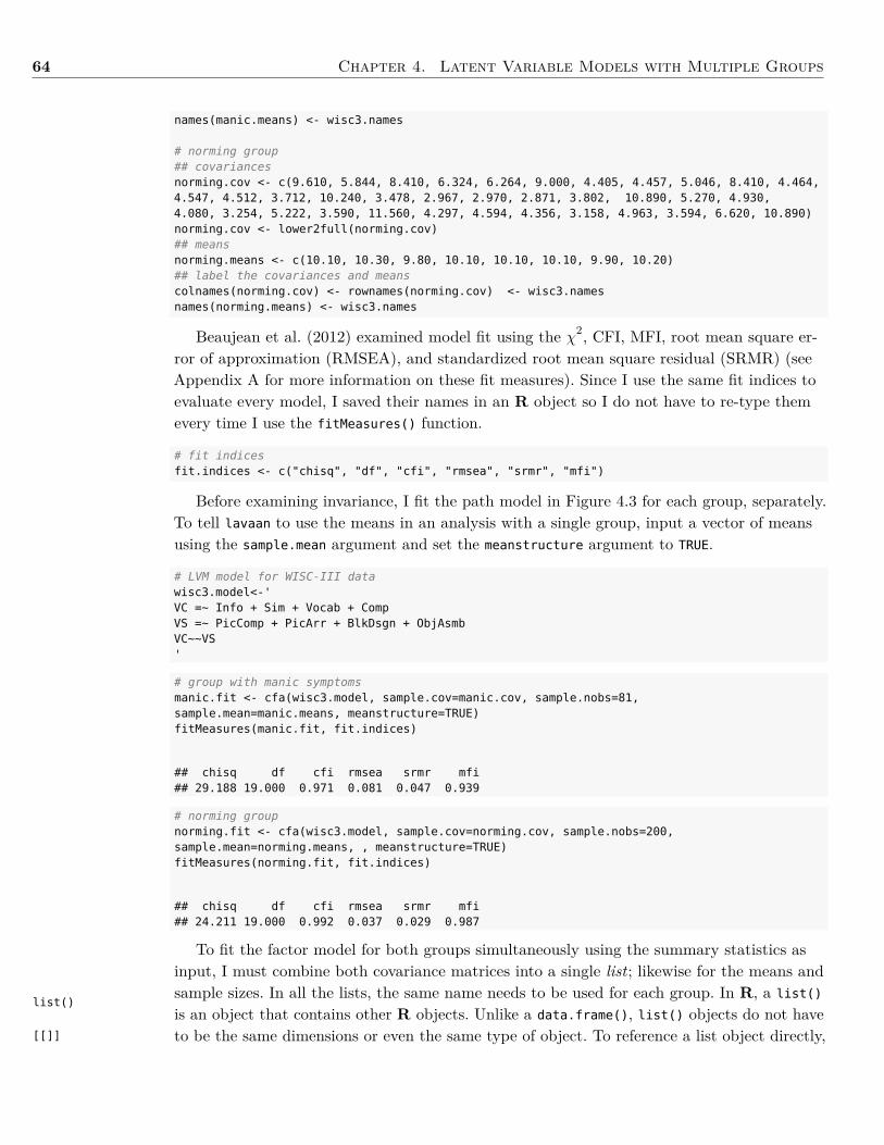
64 Chapter 4. Latent Variable Models with Multiple Groups
list()
[[]]
names(manic.means) <- wisc3.names
# norming group## covariancesnorming.cov <- c(9.610, 5.844, 8.410, 6.324, 6.264, 9.000, 4.405, 4.457, 5.046, 8.410, 4.464,4.547, 4.512, 3.712, 10.240, 3.478, 2.967, 2.970, 2.871, 3.802, 10.890, 5.270, 4.930,4.080, 3.254, 5.222, 3.590, 11.560, 4.297, 4.594, 4.356, 3.158, 4.963, 3.594, 6.620, 10.890)norming.cov <- lower2full(norming.cov)## meansnorming.means <- c(10.10, 10.30, 9.80, 10.10, 10.10, 10.10, 9.90, 10.20)## label the covariances and meanscolnames(norming.cov) <- rownames(norming.cov) <- wisc3.namesnames(norming.means) <- wisc3.names
Beaujean et al. (2012) examined model fit using the χ2, CFI, MFI, root mean square er-ror of approximation (RMSEA), and standardized root mean square residual (SRMR) (seeAppendix A for more information on these fit measures). Since I use the same fit indices toevaluate every model, I saved their names in an R object so I do not have to re-type themevery time I use the fitMeasures() function.
# fit indicesfit.indices <- c("chisq", "df", "cfi", "rmsea", "srmr", "mfi")
Before examining invariance, I fit the path model in Figure 4.3 for each group, separately.To tell lavaan to use the means in an analysis with a single group, input a vector of meansusing the sample.mean argument and set the meanstructure argument to TRUE.
# LVM model for WISC-III datawisc3.model<-'VC =~ Info + Sim + Vocab + CompVS =~ PicComp + PicArr + BlkDsgn + ObjAsmbVC~~VS'
# group with manic symptomsmanic.fit <- cfa(wisc3.model, sample.cov=manic.cov, sample.nobs=81,sample.mean=manic.means, meanstructure=TRUE)fitMeasures(manic.fit, fit.indices)
## chisq df cfi rmsea srmr mfi## 29.188 19.000 0.971 0.081 0.047 0.939
# norming groupnorming.fit <- cfa(wisc3.model, sample.cov=norming.cov, sample.nobs=200,sample.mean=norming.means, , meanstructure=TRUE)fitMeasures(norming.fit, fit.indices)
## chisq df cfi rmsea srmr mfi## 24.211 19.000 0.992 0.037 0.029 0.987
To fit the factor model for both groups simultaneously using the summary statistics asinput, I must combine both covariance matrices into a single list; likewise for the means andsample sizes. In all the lists, the same name needs to be used for each group. In R, a list()
is an object that contains other R objects. Unlike a data.frame(), list() objects do not haveto be the same dimensions or even the same type of object. To reference a list object directly,
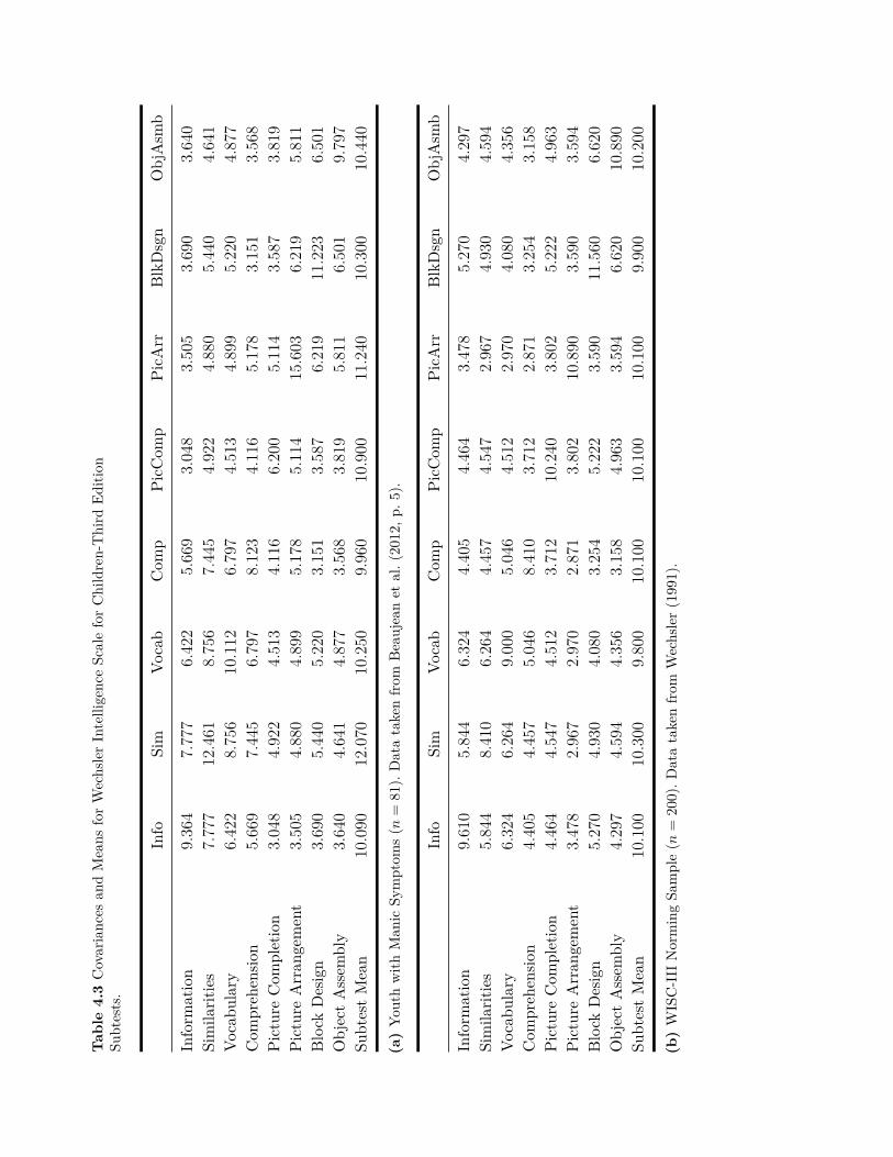
Table4.3Co variances
andMeans
forWechslerIntelligenc
eScaleforChildren-Third
Edition
Subtests.
Info
Sim
Vocab
Com
pPicC
omp
PicA
rrBlkDsgn
ObjAsm
b
Inform
ation
9.36
47.
777
6.42
25.
669
3.04
83.
505
3.69
03.
640
Simila
rities
7.77
712.4
618.
756
7.44
54.
922
4.88
05.
440
4.64
1Vo
cabu
lary
6.42
28.
756
10.1
126.
797
4.51
34.
899
5.22
04.
877
Com
prehensio
n5.
669
7.44
56.
797
8.12
34.
116
5.17
83.
151
3.56
8PictureCom
pletion
3.04
84.
922
4.51
34.
116
6.20
05.
114
3.58
73.
819
PictureArran
gement
3.50
54.
880
4.89
95.
178
5.11
415.6
036.
219
5.81
1Block
Design
3.69
05.
440
5.22
03.
151
3.58
76.
219
11.2
236.
501
ObjectAssem
bly
3.64
04.
641
4.87
73.
568
3.81
95.
811
6.50
19.
797
SubtestMean
10.0
9012.0
7010.2
509.
960
10.9
0011.2
4010.3
0010.4
40
(a)Yo
uthwith
Man
icSy
mptom
s(n
=81
).Datatakenfrom
Beaujeanet
al.(20
12,p
.5).
Info
Sim
Vocab
Com
pPicC
omp
PicA
rrBlkDsgn
ObjAsm
b
Inform
ation
9.61
05.
844
6.32
44.
405
4.46
43.
478
5.27
04.
297
Simila
rities
5.84
48.
410
6.26
44.
457
4.54
72.
967
4.93
04.
594
Vocabu
lary
6.32
46.
264
9.00
05.
046
4.51
22.
970
4.08
04.
356
Com
prehensio
n4.
405
4.45
75.
046
8.41
03.
712
2.87
13.
254
3.15
8PictureCom
pletion
4.46
44.
547
4.51
23.
712
10.2
403.
802
5.22
24.
963
PictureArran
gement
3.47
82.
967
2.97
02.
871
3.80
210.8
903.
590
3.59
4Block
Design
5.27
04.
930
4.08
03.
254
5.22
23.
590
11.5
606.
620
ObjectAssem
bly
4.29
74.
594
4.35
63.
158
4.96
33.
594
6.62
010.8
90Su
btestMean
10.1
0010.3
009.
800
10.1
0010.1
0010.1
009.
900
10.2
00
(b)W
ISC-III
NormingSa
mple(n
=20
0).D
atatakenfrom
Wechsler(199
1).
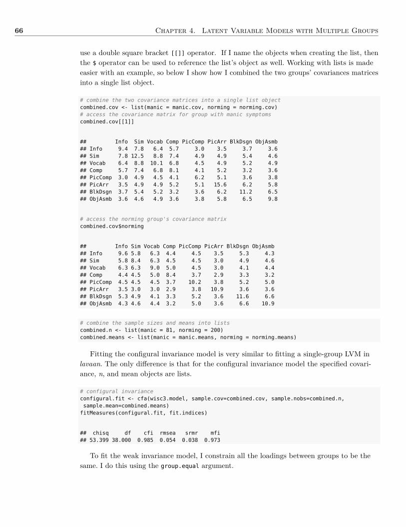
66 Chapter 4. Latent Variable Models with Multiple Groups
use a double square bracket [[]] operator. If I name the objects when creating the list, thenthe $ operator can be used to reference the list’s object as well. Working with lists is madeeasier with an example, so below I show how I combined the two groups’ covariances matricesinto a single list object.
# combine the two covariance matrices into a single list objectcombined.cov <- list(manic = manic.cov, norming = norming.cov)# access the covariance matrix for group with manic symptomscombined.cov[[1]]
## Info Sim Vocab Comp PicComp PicArr BlkDsgn ObjAsmb## Info 9.4 7.8 6.4 5.7 3.0 3.5 3.7 3.6## Sim 7.8 12.5 8.8 7.4 4.9 4.9 5.4 4.6## Vocab 6.4 8.8 10.1 6.8 4.5 4.9 5.2 4.9## Comp 5.7 7.4 6.8 8.1 4.1 5.2 3.2 3.6## PicComp 3.0 4.9 4.5 4.1 6.2 5.1 3.6 3.8## PicArr 3.5 4.9 4.9 5.2 5.1 15.6 6.2 5.8## BlkDsgn 3.7 5.4 5.2 3.2 3.6 6.2 11.2 6.5## ObjAsmb 3.6 4.6 4.9 3.6 3.8 5.8 6.5 9.8
# access the norming group's covariance matrixcombined.cov$norming
## Info Sim Vocab Comp PicComp PicArr BlkDsgn ObjAsmb## Info 9.6 5.8 6.3 4.4 4.5 3.5 5.3 4.3## Sim 5.8 8.4 6.3 4.5 4.5 3.0 4.9 4.6## Vocab 6.3 6.3 9.0 5.0 4.5 3.0 4.1 4.4## Comp 4.4 4.5 5.0 8.4 3.7 2.9 3.3 3.2## PicComp 4.5 4.5 4.5 3.7 10.2 3.8 5.2 5.0## PicArr 3.5 3.0 3.0 2.9 3.8 10.9 3.6 3.6## BlkDsgn 5.3 4.9 4.1 3.3 5.2 3.6 11.6 6.6## ObjAsmb 4.3 4.6 4.4 3.2 5.0 3.6 6.6 10.9
# combine the sample sizes and means into listscombined.n <- list(manic = 81, norming = 200)combined.means <- list(manic = manic.means, norming = norming.means)
Fitting the configural invariance model is very similar to fitting a single-group LVM inlavaan. The only difference is that for the configural invariance model the specified covari-ance, n, and mean objects are lists.
# configural invarianceconfigural.fit <- cfa(wisc3.model, sample.cov=combined.cov, sample.nobs=combined.n,sample.mean=combined.means)
fitMeasures(configural.fit, fit.indices)
## chisq df cfi rmsea srmr mfi## 53.399 38.000 0.985 0.054 0.038 0.973
To fit the weak invariance model, I constrain all the loadings between groups to be thesame. I do this using the group.equal argument.
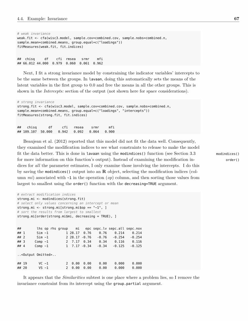
4.4. Example: Invariance 67
# weak invarianceweak.fit <- cfa(wisc3.model, sample.cov=combined.cov, sample.nobs=combined.n,sample.mean=combined.means, group.equal=c("loadings"))fitMeasures(weak.fit, fit.indices)
## chisq df cfi rmsea srmr mfi## 66.012 44.000 0.979 0.060 0.061 0.962
Next, I fit a strong invariance model by constraining the indicator variables’ intercepts tobe the same between the groups. In lavaan, doing this automatically sets the means of thelatent variables in the first group to 0.0 and free the means in all the other groups. This isshown in the Intercepts: section of the output (not shown here for space considerations).
# strong invariancestrong.fit <- cfa(wisc3.model, sample.cov=combined.cov, sample.nobs=combined.n,sample.mean=combined.means, group.equal=c("loadings", "intercepts"))fitMeasures(strong.fit, fit.indices)
## chisq df cfi rmsea srmr mfi## 109.107 50.000 0.942 0.092 0.064 0.900
Beaujean et al. (2012) reported that this model did not fit the data well. Consequently,they examined the modification indices to see what constraints to release to make the modelfit the data better. This is done in lavaan using the modindices() function (see Section 3.3for more information on this function’s output). Instead of examining the modification in-dices for all the parameter estimates, I only examine those involving the intercepts. I do thisby saving the modindices() output into an R object, selecting the modification indices (col-umn mi) associated with ~1 in the operation (op) column, and then sorting those values fromlargest to smallest using the order() function with the decreasing=TRUE argument.
# extract modification indicesstrong.mi <- modindices(strong.fit)# select only values concerning an intercept or meanstrong.mi <- strong.mi[strong.mi$op == "~1", ]# sort the results from largest to smalleststrong.mi[order(strong.mi$mi, decreasing = TRUE), ]
## lhs op rhs group mi epc sepc.lv sepc.all sepc.nox## 1 Sim ~1 1 28.17 0.76 0.76 0.214 0.214## 2 Sim ~1 2 28.17 -0.76 -0.76 -0.254 -0.254## 3 Comp ~1 2 7.17 0.34 0.34 0.116 0.116## 4 Comp ~1 1 7.17 -0.34 -0.34 -0.125 -0.125
..<Output Omitted>..
## 19 VC ~1 2 0.00 0.00 0.00 0.000 0.000## 20 VS ~1 2 0.00 0.00 0.00 0.000 0.000
It appears that the Similarities subtest is one place where a problem lies, so I remove theinvariance constraint from its intercept using the group.partial argument.
modindices()
order()
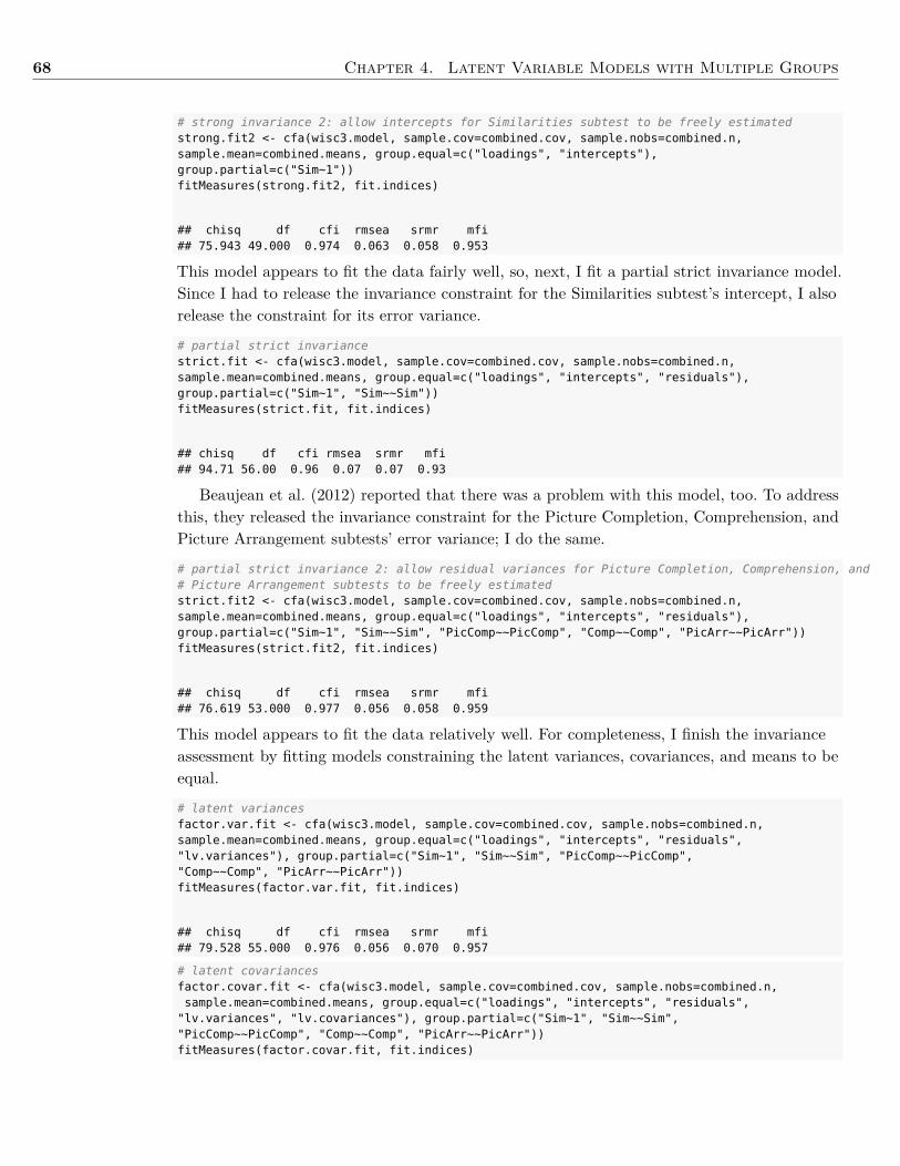
68 Chapter 4. Latent Variable Models with Multiple Groups
# strong invariance 2: allow intercepts for Similarities subtest to be freely estimatedstrong.fit2 <- cfa(wisc3.model, sample.cov=combined.cov, sample.nobs=combined.n,sample.mean=combined.means, group.equal=c("loadings", "intercepts"),group.partial=c("Sim~1"))fitMeasures(strong.fit2, fit.indices)
## chisq df cfi rmsea srmr mfi## 75.943 49.000 0.974 0.063 0.058 0.953
This model appears to fit the data fairly well, so, next, I fit a partial strict invariance model.Since I had to release the invariance constraint for the Similarities subtest’s intercept, I alsorelease the constraint for its error variance.
# partial strict invariancestrict.fit <- cfa(wisc3.model, sample.cov=combined.cov, sample.nobs=combined.n,sample.mean=combined.means, group.equal=c("loadings", "intercepts", "residuals"),group.partial=c("Sim~1", "Sim~~Sim"))fitMeasures(strict.fit, fit.indices)
## chisq df cfi rmsea srmr mfi## 94.71 56.00 0.96 0.07 0.07 0.93
Beaujean et al. (2012) reported that there was a problem with this model, too. To addressthis, they released the invariance constraint for the Picture Completion, Comprehension, andPicture Arrangement subtests’ error variance; I do the same.
# partial strict invariance 2: allow residual variances for Picture Completion, Comprehension, and# Picture Arrangement subtests to be freely estimatedstrict.fit2 <- cfa(wisc3.model, sample.cov=combined.cov, sample.nobs=combined.n,sample.mean=combined.means, group.equal=c("loadings", "intercepts", "residuals"),group.partial=c("Sim~1", "Sim~~Sim", "PicComp~~PicComp", "Comp~~Comp", "PicArr~~PicArr"))fitMeasures(strict.fit2, fit.indices)
## chisq df cfi rmsea srmr mfi## 76.619 53.000 0.977 0.056 0.058 0.959
This model appears to fit the data relatively well. For completeness, I finish the invarianceassessment by fitting models constraining the latent variances, covariances, and means to beequal.
# latent variancesfactor.var.fit <- cfa(wisc3.model, sample.cov=combined.cov, sample.nobs=combined.n,sample.mean=combined.means, group.equal=c("loadings", "intercepts", "residuals","lv.variances"), group.partial=c("Sim~1", "Sim~~Sim", "PicComp~~PicComp","Comp~~Comp", "PicArr~~PicArr"))fitMeasures(factor.var.fit, fit.indices)
## chisq df cfi rmsea srmr mfi## 79.528 55.000 0.976 0.056 0.070 0.957
# latent covariancesfactor.covar.fit <- cfa(wisc3.model, sample.cov=combined.cov, sample.nobs=combined.n,sample.mean=combined.means, group.equal=c("loadings", "intercepts", "residuals",
"lv.variances", "lv.covariances"), group.partial=c("Sim~1", "Sim~~Sim","PicComp~~PicComp", "Comp~~Comp", "PicArr~~PicArr"))fitMeasures(factor.covar.fit, fit.indices)
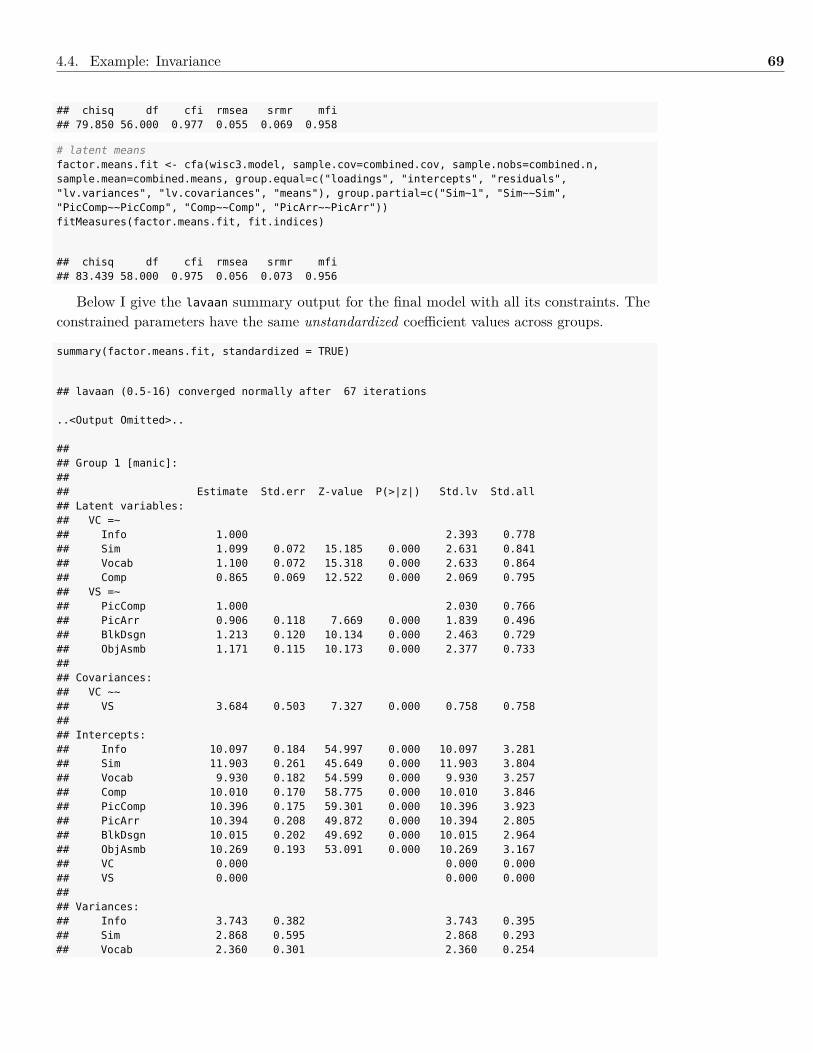
4.4. Example: Invariance 69
## chisq df cfi rmsea srmr mfi## 79.850 56.000 0.977 0.055 0.069 0.958
# latent meansfactor.means.fit <- cfa(wisc3.model, sample.cov=combined.cov, sample.nobs=combined.n,sample.mean=combined.means, group.equal=c("loadings", "intercepts", "residuals","lv.variances", "lv.covariances", "means"), group.partial=c("Sim~1", "Sim~~Sim","PicComp~~PicComp", "Comp~~Comp", "PicArr~~PicArr"))fitMeasures(factor.means.fit, fit.indices)
## chisq df cfi rmsea srmr mfi## 83.439 58.000 0.975 0.056 0.073 0.956
Below I give the lavaan summary output for the final model with all its constraints. Theconstrained parameters have the same unstandardized coefficient values across groups.
summary(factor.means.fit, standardized = TRUE)
## lavaan (0.5-16) converged normally after 67 iterations
..<Output Omitted>..
#### Group 1 [manic]:#### Estimate Std.err Z-value P(>|z|) Std.lv Std.all## Latent variables:## VC =~## Info 1.000 2.393 0.778## Sim 1.099 0.072 15.185 0.000 2.631 0.841## Vocab 1.100 0.072 15.318 0.000 2.633 0.864## Comp 0.865 0.069 12.522 0.000 2.069 0.795## VS =~## PicComp 1.000 2.030 0.766## PicArr 0.906 0.118 7.669 0.000 1.839 0.496## BlkDsgn 1.213 0.120 10.134 0.000 2.463 0.729## ObjAsmb 1.171 0.115 10.173 0.000 2.377 0.733#### Covariances:## VC ~~## VS 3.684 0.503 7.327 0.000 0.758 0.758#### Intercepts:## Info 10.097 0.184 54.997 0.000 10.097 3.281## Sim 11.903 0.261 45.649 0.000 11.903 3.804## Vocab 9.930 0.182 54.599 0.000 9.930 3.257## Comp 10.010 0.170 58.775 0.000 10.010 3.846## PicComp 10.396 0.175 59.301 0.000 10.396 3.923## PicArr 10.394 0.208 49.872 0.000 10.394 2.805## BlkDsgn 10.015 0.202 49.692 0.000 10.015 2.964## ObjAsmb 10.269 0.193 53.091 0.000 10.269 3.167## VC 0.000 0.000 0.000## VS 0.000 0.000 0.000#### Variances:## Info 3.743 0.382 3.743 0.395## Sim 2.868 0.595 2.868 0.293## Vocab 2.360 0.301 2.360 0.254
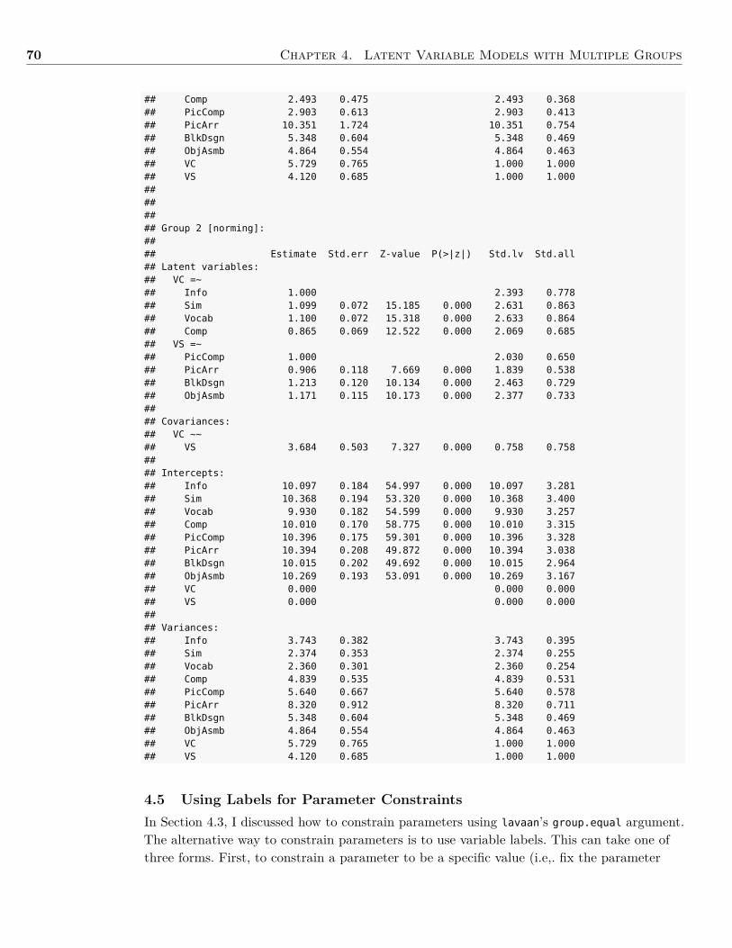
70 Chapter 4. Latent Variable Models with Multiple Groups
## Comp 2.493 0.475 2.493 0.368## PicComp 2.903 0.613 2.903 0.413## PicArr 10.351 1.724 10.351 0.754## BlkDsgn 5.348 0.604 5.348 0.469## ObjAsmb 4.864 0.554 4.864 0.463## VC 5.729 0.765 1.000 1.000## VS 4.120 0.685 1.000 1.000######## Group 2 [norming]:#### Estimate Std.err Z-value P(>|z|) Std.lv Std.all## Latent variables:## VC =~## Info 1.000 2.393 0.778## Sim 1.099 0.072 15.185 0.000 2.631 0.863## Vocab 1.100 0.072 15.318 0.000 2.633 0.864## Comp 0.865 0.069 12.522 0.000 2.069 0.685## VS =~## PicComp 1.000 2.030 0.650## PicArr 0.906 0.118 7.669 0.000 1.839 0.538## BlkDsgn 1.213 0.120 10.134 0.000 2.463 0.729## ObjAsmb 1.171 0.115 10.173 0.000 2.377 0.733#### Covariances:## VC ~~## VS 3.684 0.503 7.327 0.000 0.758 0.758#### Intercepts:## Info 10.097 0.184 54.997 0.000 10.097 3.281## Sim 10.368 0.194 53.320 0.000 10.368 3.400## Vocab 9.930 0.182 54.599 0.000 9.930 3.257## Comp 10.010 0.170 58.775 0.000 10.010 3.315## PicComp 10.396 0.175 59.301 0.000 10.396 3.328## PicArr 10.394 0.208 49.872 0.000 10.394 3.038## BlkDsgn 10.015 0.202 49.692 0.000 10.015 2.964## ObjAsmb 10.269 0.193 53.091 0.000 10.269 3.167## VC 0.000 0.000 0.000## VS 0.000 0.000 0.000#### Variances:## Info 3.743 0.382 3.743 0.395## Sim 2.374 0.353 2.374 0.255## Vocab 2.360 0.301 2.360 0.254## Comp 4.839 0.535 4.839 0.531## PicComp 5.640 0.667 5.640 0.578## PicArr 8.320 0.912 8.320 0.711## BlkDsgn 5.348 0.604 5.348 0.469## ObjAsmb 4.864 0.554 4.864 0.463## VC 5.729 0.765 1.000 1.000## VS 4.120 0.685 1.000 1.000
4.5 Using Labels for Parameter ConstraintsIn Section 4.3, I discussed how to constrain parameters using lavaan’s group.equal argument.The alternative way to constrain parameters is to use variable labels. This can take one ofthree forms. First, to constrain a parameter to be a specific value (i.e,. fix the parameter
4.6. Example: Genetically Informative Design 71
estimate), premultiply the parameter by the desired value. For example, to constrain theloading of V2:
F1 =~ V1 + 3*V2 + V3
Second, to constrain a parameter to be greater/less than a value, premultiply the label bythe parameter, then in a separate line give the inequality. For example, to constrain the vari-ance of V1 to be greater than 0:
V1 ~~ a*V1a > 0
Third, to estimate a parameter, but constrain it to be the same value among multiple groups,use the same label in all the groups. To do this, use the concatenate function, c(), to applymultiple labels.6 For example, to constrain the loading of V2 to be the same value betweentwo groups:
F1 =~ V1 + c(a,a)*V2 + V3
4.6 Example: Genetically Informative DesignIn Section 4.1, I stated there were two purposes for including multiple groups in a LVM. Thefirst was to examine invariance. The second purpose is when the estimation of a parameterrequires data from two or more unique groups. This is commonly done with genetically in-formative designs, as is common in the field of behavior genetics. Behavior genetic (BG)models examine genetic and environmental influences on physical or behavioral traits (i.e., aphenotype). The research designs in this field use natural experiments to study these influ-ences, such as twins reared in different environments and children in adopted families.
In BG models, the genetic influence on a phenotype is decomposed into: (a) additive ef-fects of alleles at various loci (A) (this is sometimes called narrow heritability); and (b) non-ad-ditive effects (D), such as allele dominance.The combination of A and D is called the broadheritability. Likewise, environmental influence on the phenotype is decomposed into: (a) ef-fects due to a shared environment (C ) (i.e., between-family effects), such as being raisedby the same parents in the same house; and (b) effects due to a non-shared environment(E) (i.e., within-family effects), such as having different peers or attending different schools.These non-shared effects include random environmental events (e.g., getting into automobileaccident) as well as random measurement events (i.e, measurement error). For readers inter-ested in such models, Plomin, DeFries, McClearn, and McGuffin (2008) provide an excellentintroductory text.
Figure 4.4 contains a path model for a BG analysis of a single phenotype, P, measured inboth identical/monozygotic (MZ) and fraternal/dizygotic (DZ) twins raised together. Themodel has seven latent variables, but there are only two indicator variables: the phenotypemeasured in twin 1 (P1) and in twin 2 (P2). This is obviously an underidentified model, so Ineed to place constraints on the parameter estimates to obtain unique estimates. For the LVs
Behavior Genetics
6A second way to constrain parameters between groups within the model is to specify m separate modelsfor your m groups, and give the parameters to be constrained the same label. For an example, see my answerto Exercise 4.1.b.
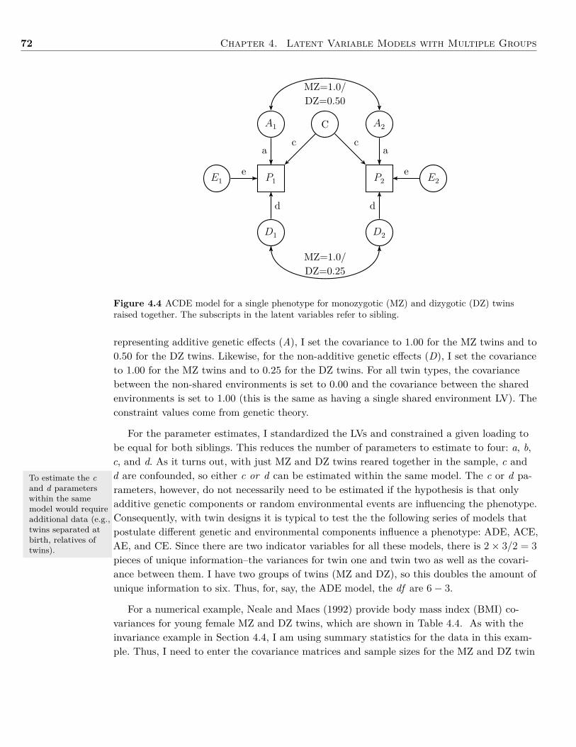
72 Chapter 4. Latent Variable Models with Multiple Groups
CA1 A2
P1 P2E1 E2
D1 D2
MZ=1.0/DZ=0.25
MZ=1.0/DZ=0.50
a ac c
e e
d d
Figure 4.4 ACDE model for a single phenotype for monozygotic (MZ) and dizygotic (DZ) twinsraised together. The subscripts in the latent variables refer to sibling.
To estimate the cand d parameterswithin the samemodel would requireadditional data (e.g.,twins separated atbirth, relatives oftwins).
representing additive genetic effects (A), I set the covariance to 1.00 for the MZ twins and to0.50 for the DZ twins. Likewise, for the non-additive genetic effects (D), I set the covarianceto 1.00 for the MZ twins and to 0.25 for the DZ twins. For all twin types, the covariancebetween the non-shared environments is set to 0.00 and the covariance between the sharedenvironments is set to 1.00 (this is the same as having a single shared environment LV). Theconstraint values come from genetic theory.
For the parameter estimates, I standardized the LVs and constrained a given loading tobe equal for both siblings. This reduces the number of parameters to estimate to four: a, b,c, and d. As it turns out, with just MZ and DZ twins reared together in the sample, c andd are confounded, so either c or d can be estimated within the same model. The c or d pa-rameters, however, do not necessarily need to be estimated if the hypothesis is that onlyadditive genetic components or random environmental events are influencing the phenotype.Consequently, with twin designs it is typical to test the the following series of models thatpostulate different genetic and environmental components influence a phenotype: ADE, ACE,AE, and CE. Since there are two indicator variables for all these models, there is 2× 3/2 = 3pieces of unique information–the variances for twin one and twin two as well as the covari-ance between them. I have two groups of twins (MZ and DZ), so this doubles the amount ofunique information to six. Thus, for, say, the ADE model, the df are 6− 3.
For a numerical example, Neale and Maes (1992) provide body mass index (BMI) co-variances for young female MZ and DZ twins, which are shown in Table 4.4. As with theinvariance example in Section 4.4, I am using summary statistics for the data in this exam-ple. Thus, I need to enter the covariance matrices and sample sizes for the MZ and DZ twin
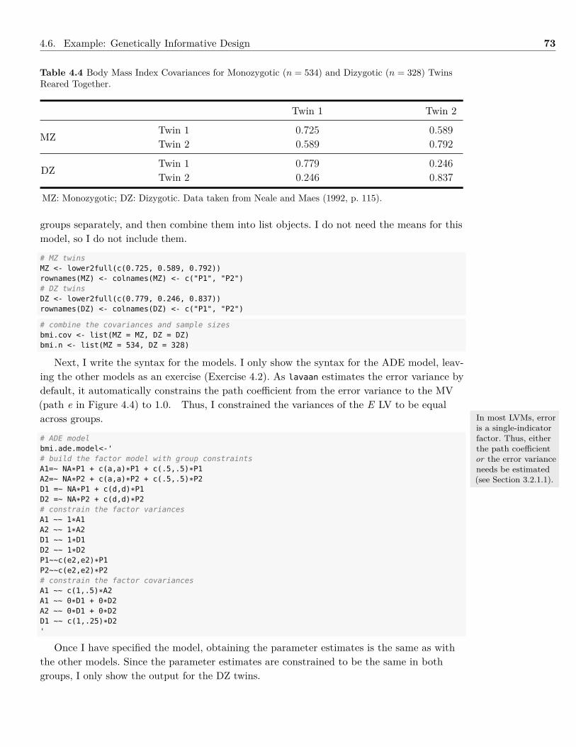
4.6. Example: Genetically Informative Design 73
Table 4.4 Body Mass Index Covariances for Monozygotic (n = 534) and Dizygotic (n = 328) TwinsReared Together.
Twin 1 Twin 2
MZ Twin 1 0.725 0.589Twin 2 0.589 0.792
DZ Twin 1 0.779 0.246Twin 2 0.246 0.837
MZ: Monozygotic; DZ: Dizygotic. Data taken from Neale and Maes (1992, p. 115).
groups separately, and then combine them into list objects. I do not need the means for thismodel, so I do not include them.
# MZ twinsMZ <- lower2full(c(0.725, 0.589, 0.792))rownames(MZ) <- colnames(MZ) <- c("P1", "P2")# DZ twinsDZ <- lower2full(c(0.779, 0.246, 0.837))rownames(DZ) <- colnames(DZ) <- c("P1", "P2")
# combine the covariances and sample sizesbmi.cov <- list(MZ = MZ, DZ = DZ)bmi.n <- list(MZ = 534, DZ = 328)
Next, I write the syntax for the models. I only show the syntax for the ADE model, leav-ing the other models as an exercise (Exercise 4.2). As lavaan estimates the error variance bydefault, it automatically constrains the path coefficient from the error variance to the MV(path e in Figure 4.4) to 1.0. Thus, I constrained the variances of the E LV to be equalacross groups.
# ADE modelbmi.ade.model<-'# build the factor model with group constraintsA1=~ NA*P1 + c(a,a)*P1 + c(.5,.5)*P1A2=~ NA*P2 + c(a,a)*P2 + c(.5,.5)*P2D1 =~ NA*P1 + c(d,d)*P1D2 =~ NA*P2 + c(d,d)*P2# constrain the factor variancesA1 ~~ 1*A1A2 ~~ 1*A2D1 ~~ 1*D1D2 ~~ 1*D2P1~~c(e2,e2)*P1P2~~c(e2,e2)*P2# constrain the factor covariancesA1 ~~ c(1,.5)*A2A1 ~~ 0*D1 + 0*D2A2 ~~ 0*D1 + 0*D2D1 ~~ c(1,.25)*D2'
Once I have specified the model, obtaining the parameter estimates is the same as withthe other models. Since the parameter estimates are constrained to be the same in bothgroups, I only show the output for the DZ twins.
In most LVMs, erroris a single-indicatorfactor. Thus, eitherthe path coefficientor the error varianceneeds be estimated(see Section 3.2.1.1).
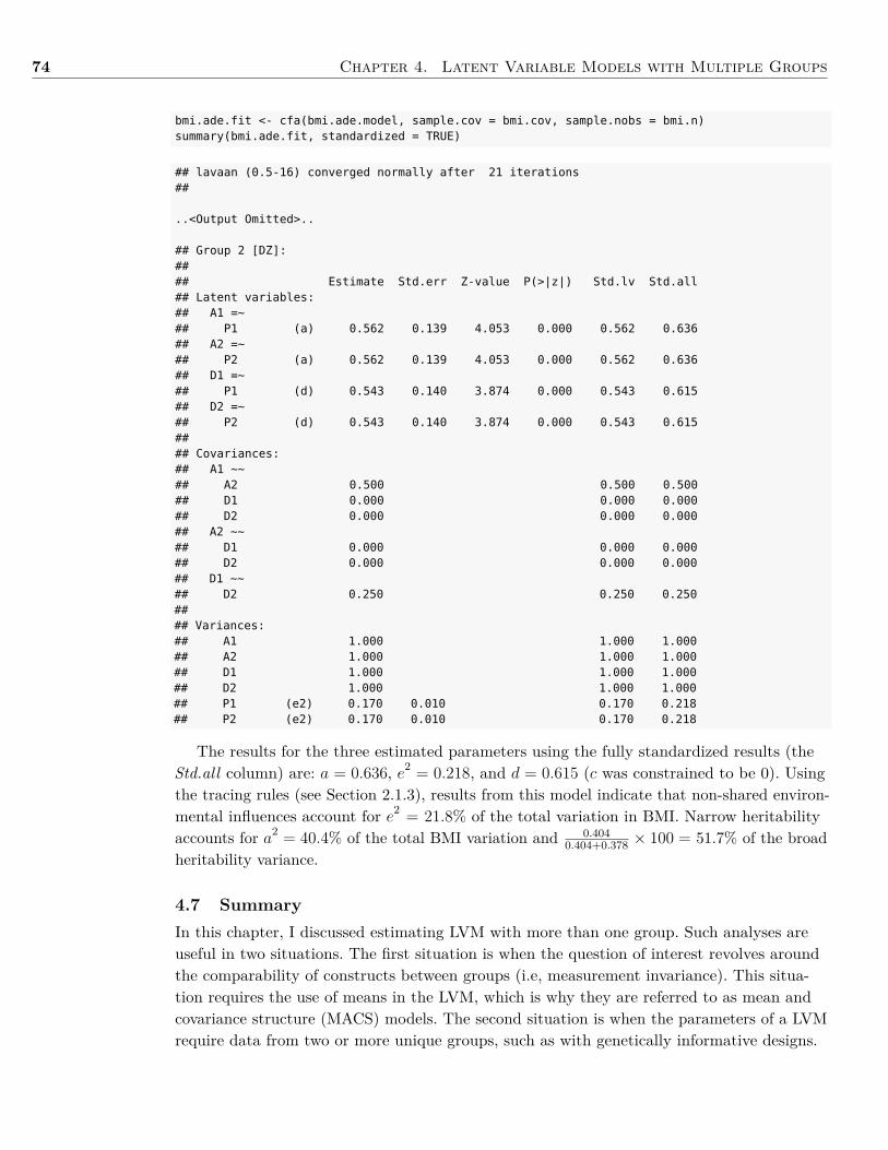
74 Chapter 4. Latent Variable Models with Multiple Groups
bmi.ade.fit <- cfa(bmi.ade.model, sample.cov = bmi.cov, sample.nobs = bmi.n)summary(bmi.ade.fit, standardized = TRUE)
## lavaan (0.5-16) converged normally after 21 iterations##
..<Output Omitted>..
## Group 2 [DZ]:#### Estimate Std.err Z-value P(>|z|) Std.lv Std.all## Latent variables:## A1 =~## P1 (a) 0.562 0.139 4.053 0.000 0.562 0.636## A2 =~## P2 (a) 0.562 0.139 4.053 0.000 0.562 0.636## D1 =~## P1 (d) 0.543 0.140 3.874 0.000 0.543 0.615## D2 =~## P2 (d) 0.543 0.140 3.874 0.000 0.543 0.615#### Covariances:## A1 ~~## A2 0.500 0.500 0.500## D1 0.000 0.000 0.000## D2 0.000 0.000 0.000## A2 ~~## D1 0.000 0.000 0.000## D2 0.000 0.000 0.000## D1 ~~## D2 0.250 0.250 0.250#### Variances:## A1 1.000 1.000 1.000## A2 1.000 1.000 1.000## D1 1.000 1.000 1.000## D2 1.000 1.000 1.000## P1 (e2) 0.170 0.010 0.170 0.218## P2 (e2) 0.170 0.010 0.170 0.218
The results for the three estimated parameters using the fully standardized results (theStd.all column) are: a = 0.636, e2 = 0.218, and d = 0.615 (c was constrained to be 0). Usingthe tracing rules (see Section 2.1.3), results from this model indicate that non-shared environ-mental influences account for e2 = 21.8% of the total variation in BMI. Narrow heritabilityaccounts for a2 = 40.4% of the total BMI variation and 0.404
0.404+0.378 × 100 = 51.7% of the broadheritability variance.
4.7 SummaryIn this chapter, I discussed estimating LVM with more than one group. Such analyses areuseful in two situations. The first situation is when the question of interest revolves aroundthe comparability of constructs between groups (i.e, measurement invariance). This situa-tion requires the use of means in the LVM, which is why they are referred to as mean andcovariance structure (MACS) models. The second situation is when the parameters of a LVMrequire data from two or more unique groups, such as with genetically informative designs.
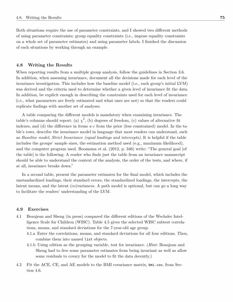
4.8. Writing the Results 75
Both situations require the use of parameter constraints, and I showed two different methodsof using parameter constraints: group equality constraints (i.e., impose equality constraintson a whole set of parameter estimates) and using parameter labels. I finished the discussionof each situations by working through an example.
4.8 Writing the ResultsWhen reporting results from a multiple group analysis, follow the guidelines in Section 3.6.In addition, when assessing invariance, document all the decisions made for each level of theinvariance investigation. This includes how the baseline model (i.e., each group’s initial LVM)was derived and the criteria used to determine whether a given level of invariance fit the data.In addition, be explicit enough in describing the constraints used for each level of invariance(i.e., what parameters are freely estimated and what ones are not) so that the readers couldreplicate findings with another set of analyses.
A table comparing the different models is mandatory when examining invariance. Thetable’s columns should report: (a) χ2, (b) degrees of freedom, (c) values of alternative fitindexes, and (d) the difference in items a-c from the prior (less constrained) model. In the ta-ble’s rows, describe the invariance model in language that most readers can understand, suchas Baseline model, Strict Invariance (equal loadings and intercepts). It is helpful if the tableincludes the groups’ sample sizes, the estimation method used (e.g., maximum likelihood),and the computer program used. Boomsma et al. (2012, p. 346) write: “The general goal [ofthe table] is the following: A reader who finds just the table from an invariance manuscriptshould be able to understand the context of the analysis, the order of the tests, and where, ifat all, invariance breaks down.”
In a second table, present the parameter estimates for the final model, which includes theunstandardized loadings, their standard errors, the standardized loadings, the intercepts, thelatent means, and the latent (co)variances. A path model is optional, but can go a long wayto facilitate the readers’ understanding of the LVM.
4.9 Exercises4.1 Beaujean and Sheng (in press) compared the different editions of the Wechsler Intel-
ligence Scale for Children (WISC). Table 4.5 gives the selected WISC subtest correla-tions, means, and standard deviations for the 7-year-old age group.4.1.a Enter the correlations, means, and standard deviations for all four editions. Then,
combine them into named list objects.4.1.b Using edition as the grouping variable, test for invariance. (Hint: Beaujean and
Sheng had to free some parameter estimates from being invariant as well as allowsome residuals to covary for the model to fit the data decently.)
4.2 Fit the ACE, CE, and AE models to the BMI covariance matrix, bmi.cov, from Sec-tion 4.6.
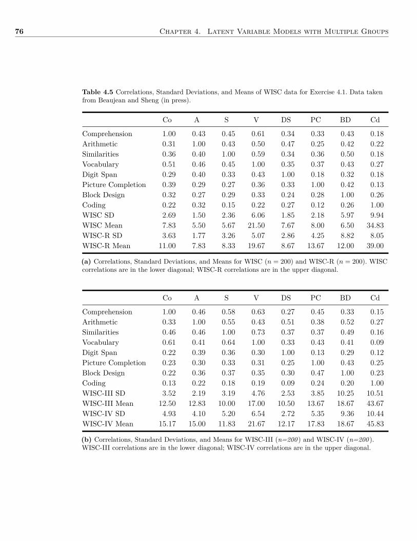
76 Chapter 4. Latent Variable Models with Multiple Groups
Table 4.5 Correlations, Standard Deviations, and Means of WISC data for Exercise 4.1. Data takenfrom Beaujean and Sheng (in press).
Co A S V DS PC BD Cd
Comprehension 1.00 0.43 0.45 0.61 0.34 0.33 0.43 0.18Arithmetic 0.31 1.00 0.43 0.50 0.47 0.25 0.42 0.22Similarities 0.36 0.40 1.00 0.59 0.34 0.36 0.50 0.18Vocabulary 0.51 0.46 0.45 1.00 0.35 0.37 0.43 0.27Digit Span 0.29 0.40 0.33 0.43 1.00 0.18 0.32 0.18Picture Completion 0.39 0.29 0.27 0.36 0.33 1.00 0.42 0.13Block Design 0.32 0.27 0.29 0.33 0.24 0.28 1.00 0.26Coding 0.22 0.32 0.15 0.22 0.27 0.12 0.26 1.00WISC SD 2.69 1.50 2.36 6.06 1.85 2.18 5.97 9.94WISC Mean 7.83 5.50 5.67 21.50 7.67 8.00 6.50 34.83WISC-R SD 3.63 1.77 3.26 5.07 2.86 4.25 8.82 8.05WISC-R Mean 11.00 7.83 8.33 19.67 8.67 13.67 12.00 39.00
(a) Correlations, Standard Deviations, and Means for WISC (n = 200) and WISC-R (n = 200). WISCcorrelations are in the lower diagonal; WISC-R correlations are in the upper diagonal.
Co A S V DS PC BD Cd
Comprehension 1.00 0.46 0.58 0.63 0.27 0.45 0.33 0.15Arithmetic 0.33 1.00 0.55 0.43 0.51 0.38 0.52 0.27Similarities 0.46 0.46 1.00 0.73 0.37 0.37 0.49 0.16Vocabulary 0.61 0.41 0.64 1.00 0.33 0.43 0.41 0.09Digit Span 0.22 0.39 0.36 0.30 1.00 0.13 0.29 0.12Picture Completion 0.23 0.30 0.33 0.31 0.25 1.00 0.43 0.25Block Design 0.22 0.36 0.37 0.35 0.30 0.47 1.00 0.23Coding 0.13 0.22 0.18 0.19 0.09 0.24 0.20 1.00WISC-III SD 3.52 2.19 3.19 4.76 2.53 3.85 10.25 10.51WISC-III Mean 12.50 12.83 10.00 17.00 10.50 13.67 18.67 43.67WISC-IV SD 4.93 4.10 5.20 6.54 2.72 5.35 9.36 10.44WISC-IV Mean 15.17 15.00 11.83 21.67 12.17 17.83 18.67 45.83
(b) Correlations, Standard Deviations, and Means for WISC-III (n=200 ) and WISC-IV (n=200 ).WISC-III correlations are in the lower diagonal; WISC-IV correlations are in the upper diagonal.
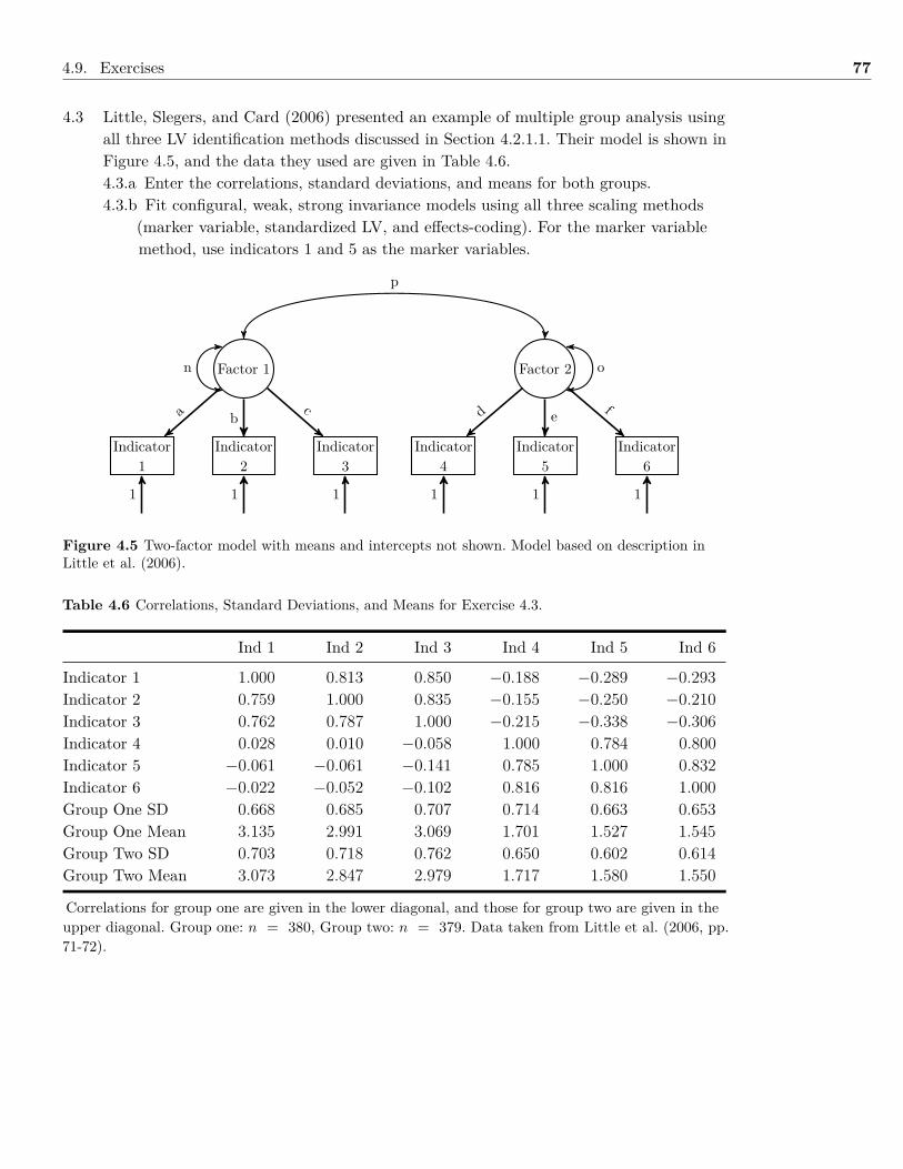
4.9. Exercises 77
4.3 Little, Slegers, and Card (2006) presented an example of multiple group analysis usingall three LV identification methods discussed in Section 4.2.1.1. Their model is shown inFigure 4.5, and the data they used are given in Table 4.6.4.3.a Enter the correlations, standard deviations, and means for both groups.4.3.b Fit configural, weak, strong invariance models using all three scaling methods
(marker variable, standardized LV, and effects-coding). For the marker variablemethod, use indicators 1 and 5 as the marker variables.
Factor 1 Factor 2
Indicator2
Indicator3
Indicator1
Indicator5
Indicator4
Indicator6
a bc d e f
1 1 1 1 1 1
p
n o
Figure 4.5 Two-factor model with means and intercepts not shown. Model based on description inLittle et al. (2006).
Table 4.6 Correlations, Standard Deviations, and Means for Exercise 4.3.
Ind 1 Ind 2 Ind 3 Ind 4 Ind 5 Ind 6
Indicator 1 1.000 0.813 0.850 −0.188 −0.289 −0.293Indicator 2 0.759 1.000 0.835 −0.155 −0.250 −0.210Indicator 3 0.762 0.787 1.000 −0.215 −0.338 −0.306Indicator 4 0.028 0.010 −0.058 1.000 0.784 0.800Indicator 5 −0.061 −0.061 −0.141 0.785 1.000 0.832Indicator 6 −0.022 −0.052 −0.102 0.816 0.816 1.000Group One SD 0.668 0.685 0.707 0.714 0.663 0.653Group One Mean 3.135 2.991 3.069 1.701 1.527 1.545Group Two SD 0.703 0.718 0.762 0.650 0.602 0.614Group Two Mean 3.073 2.847 2.979 1.717 1.580 1.550
Correlations for group one are given in the lower diagonal, and those for group two are given in theupper diagonal. Group one: n = 380, Group two: n = 379. Data taken from Little et al. (2006, pp.71-72).
78 Chapter 4. Latent Variable Models with Multiple Groups
4.10 References & Further ReadingsBeaujean, A. A., Freeman, M. J., Youngstrom, E., & Carlson, G. (2012). The structure of
cognitive abilities in youths with manic symptoms: A factorial invariance study.Assessment, 19 , 462-471. doi: 10.1177/1073191111399037
Beaujean, A. A., & Sheng, Y. (in press). Assessing the Flynn effect in the Wechsler scales.Journal of Individual Differences.
Boomsma, A., Hoyle, R. H., & Panter, A. T. (2012). The structural equation modelingresearch report. In R. H. Hoyle (Ed.), Handbook of structural equation modeling. NewYork, NY: Guilford.
Horn, J. L., & McArdle, J. J. (1992). A practical and theoretical guide to measurementinvariance in aging research. Experimental Aging Research, 18 , 117-144.
Little, T. D. (1997). Mean and covariance structures (MACS) analyses of cross-cultural data:Practical and theoretical issues. Multivariate Behavioral Research, 32 , 53-76. doi:10.1207/s15327906mbr3201_3
Little, T. D., Card, N. A., Slegers, D. W., & Ledford, E. C. (2007). Representing contextualeffects in multiple-group MACS models. In T. D. Little, J. A. Bovaird, & N. A. Card(Eds.), Modeling ecological and contextual effects in longitudinal studies (pp. 121–147).Mahwah, NJ: Lawrence Erlbaum Associates.
Little, T. D., Slegers, D. W., & Card, N. A. (2006). A non-arbitrary method of identifying andscaling latent variables in SEM and MACS models. Structural Equation Modeling: AMultidisciplinary Journal, 13 , 59-72. doi: 10.1207/s15328007sem1301_3
Meade, A. W., Johnson, E. C., & Braddy, P. W. (2008). Power and sensitivity of alternativefit indices in tests of measurement invariance. Journal of Applied Psychology, 93 ,568-592. doi: 10.1037/0021-9010.93.3.568
Millsap, R. E. (2011). Statistical approaches to measurement invariance. New York, NY:Routledge.
Neale, M. C., & Maes, H. H. M. (1992). Methodology for genetic studies of twins and families.Dordrecht, The Netherlands: Kluwer Academic Publishers.
Plomin, R., DeFries, J. C., McClearn, G. E., & McGuffin, P. (2008). Behavioral genetics (5thed.). New York: Worth.
Rutter, M. (2007). Proceeding from observed correlation to causal inference: The use ofnatural experiments. Perspectives on Psychological Science, 2 , 377-395. doi:10.1111/j.1745-6916.2007.00050.x
Steenkamp, J.-B. E. M., & Baumgartner, H. (1998). Assessing measurement invariance incross-national consumer research. Journal of Consumer Research, 25 , 78-107. doi:10.1086/209528
Vandenberg, R. J., & Lance, C. E. (2000). A review and synthesis of the measurementinvariance literature: Suggestions, practices, and recommendations for organizationalresearch. Organizational Research Methods, 3 , 4-70. doi: 10.1177/109442810031002
Wechsler, D. (1991). Wechsler intelligence scale for children (3rd ed.). San Antonio, TX: ThePsychological Corporation.
5 | Models with Multiple TimePeriods
Chapter Contents5.1 Background . . . . . . . . . . . . . . . . . . . . . . . . . . . . . . . . . . . . 79
5.1.1 Latent Curve Models in lavaan . . . . . . . . . . . . . . . . . . . . . 805.2 Example: Latent Curve Model . . . . . . . . . . . . . . . . . . . . . . . . . . 805.3 Latent Curve Model Extensions . . . . . . . . . . . . . . . . . . . . . . . . . 84
5.3.1 Adding Covariates . . . . . . . . . . . . . . . . . . . . . . . . . . . . 845.3.2 Multi-Group Models . . . . . . . . . . . . . . . . . . . . . . . . . . . 875.3.3 Alternative Ways to Specify the Latent Intercept and Slope . . . . . 87
5.4 Summary . . . . . . . . . . . . . . . . . . . . . . . . . . . . . . . . . . . . . . 885.5 Writing the Results . . . . . . . . . . . . . . . . . . . . . . . . . . . . . . . . 885.6 Exercises . . . . . . . . . . . . . . . . . . . . . . . . . . . . . . . . . . . . . . 895.7 References & Further Readings . . . . . . . . . . . . . . . . . . . . . . . . . . 92
5.1 BackgroundThis far, all of the models I have considered used data measured at a single time period.LVMs are versatile, though, and can handle data that has been measured at multiple timeperiods (i.e., repeated measures). There are a variety of ways to analyze such data, such asgrowth models, multilevel models, and random regression/mixed-effects models. When usinga LVM, though, the model is typically called a latent growth curve model or simply a latentcurve model (LCM).
In LCMs, each respondent in the sample has his or her own trajectory of change over timeon the measured variable(s). Thus, characteristics of the trajectory (i.e., slope, intercept) canvary across individuals. To allow this variation, the parameters are modeled as LVs. I callthese variables latent intercept and latent slope, so as not to confuse them with the manifestintercepts I discussed in Section 4.2.1. Like any other LV, the latent intercept and latentslope can be exogenous or endogenous. Figure 5.1 contains a path model of a LCM with dataacross four time periods.
LCMs provide a great amount of flexibility in examining change over time. Moreover,more traditional forms of modeling growth (e.g., repeated measures ANOVA), as well asmore modern forms of modeling growth (e.g., multilevel model), can be parametrized as aLCM. What sets apart LCM from other methods of analyzing change is that LCMs are ex-plicit in modeling the latent slope and latent intercept’s covariances, as well as modeling thestructure of the error variances. Moreover, like all LVMs, LCMs can examine how differentmodels fit the data.
Latent CurveModel
79
80 Chapter 5. Models with Multiple Time Periods
Random Effects
growth()
In the LVM models I have examined thus far, the loadings were usually estimated, unlessthey were constrained for identification or to examine invariance. In LCM, typically all theloadings are fixed. For the latent intercept, the loadings are fixed to 1.0, which indicates thelatent intercept has equal influence on the indicator variables across all waves of data collec-tion. The latent slope’s loadings can have a variety of values, increasing from one time pointto another, although they are somewhat dependent on the time between data collections andthe nature of the hypothesized growth. The best values to start with are 0.0 for the first timepoint and then have the values increase by 1.0 for the subsequent loadings (i.e., 0.0, 1.0, 2.0,3.0), which reflects an equal amount of time passing between data collection time periods.Starting with 0.0 gives the mean of the latent intercept the interpretation of being the meanvalue of the outcome variable at the first time point.
LCMs not only need to account for the means of the manifest variables, but they needto account for mean changes as well. Thus, they need to include the manifest variables’ in-tercepts as well as the latent means (see Section 4.2.1). Usually, the manifest intercepts areconstrained to be 0.0, which makes the manifest variables’ means modeled entirely by the la-tent means.1 The residual (co)variances and latent (co)variances are modeled as usual, unlessthere is a need to constrain their values.
Bollen and Curran (2006) give three questions to ask when initially creating a LCM:
1. What is the average trajectory for all respondents? Stated differently: (a) what is theinitial level of the variable (i.e., mean); (b) does the variable change over time; and, ifso, (c) what is the form of the change (e.g., linear, quadratic)?
2. Is the average trajectory sufficient, or is there enough variability between observationsto warrant allowing distinct trajectories? In other words, does the latent intercept orlatent slope need to have a variance term or can the variance be constrained to 0.0?These latent slope and latent intercept variances are sometimes called random ef-fects.
3. If distinct trajectories are needed (i.e., the latent slope or latent intercept has variabil-ity), are there variables that can predict them? That is, do other variables need to beadded to the LCM to explain the latent intercept or latent slope variability?
5.1.1 Latent Curve Models in lavaan
The easiest way to specify a LCM in lavaan is to use the growth() function. The growth()
function is very similar to the sem() function, but it assumes there are means and inter-cepts in the model, with the observed intercepts fixed to zero and the latent means freelyestimated.
5.2 Example: Latent Curve ModelThe data are crime rates in various New York and Pennsylvania communities, measured atfour equidistant time periods across eight months in 1995.2 Summary statistics are given in
1An alternative parameterization is to set the latent means equal to 0.0 and estimate the intercepts in-stead.
2The outcome variable is actually the logarithm of the crime rates. The authors transformed the variablesto have them better approximate a normal distribution.
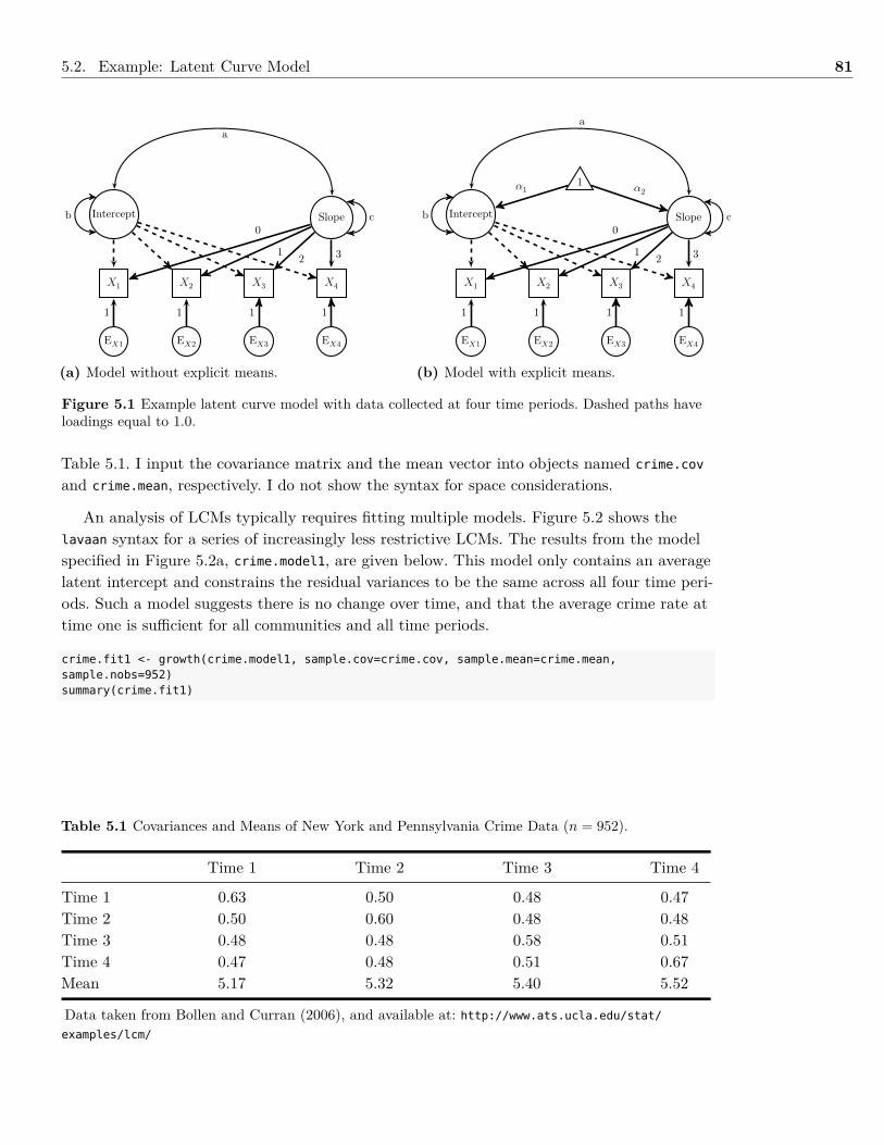
5.2. Example: Latent Curve Model 81
X3X2X1 X4
EX1 EX2 EX3 EX4
1 1 1 1
Intercept Slope0
1 2 3
a
b c
(a) Model without explicit means.
X3X2X1 X4
EX1 EX2 EX3 EX4
1 1 1 1
Intercept Slope
1α1 α2
0
1 2 3
a
b c
(b) Model with explicit means.
Figure 5.1 Example latent curve model with data collected at four time periods. Dashed paths haveloadings equal to 1.0.
Table 5.1. I input the covariance matrix and the mean vector into objects named crime.cov
and crime.mean, respectively. I do not show the syntax for space considerations.
An analysis of LCMs typically requires fitting multiple models. Figure 5.2 shows thelavaan syntax for a series of increasingly less restrictive LCMs. The results from the modelspecified in Figure 5.2a, crime.model1, are given below. This model only contains an averagelatent intercept and constrains the residual variances to be the same across all four time peri-ods. Such a model suggests there is no change over time, and that the average crime rate attime one is sufficient for all communities and all time periods.
crime.fit1 <- growth(crime.model1, sample.cov=crime.cov, sample.mean=crime.mean,sample.nobs=952)summary(crime.fit1)
Table 5.1 Covariances and Means of New York and Pennsylvania Crime Data (n = 952).
Time 1 Time 2 Time 3 Time 4
Time 1 0.63 0.50 0.48 0.47Time 2 0.50 0.60 0.48 0.48Time 3 0.48 0.48 0.58 0.51Time 4 0.47 0.48 0.51 0.67Mean 5.17 5.32 5.40 5.52
Data taken from Bollen and Curran (2006), and available at: http://www.ats.ucla.edu/stat/examples/lcm/
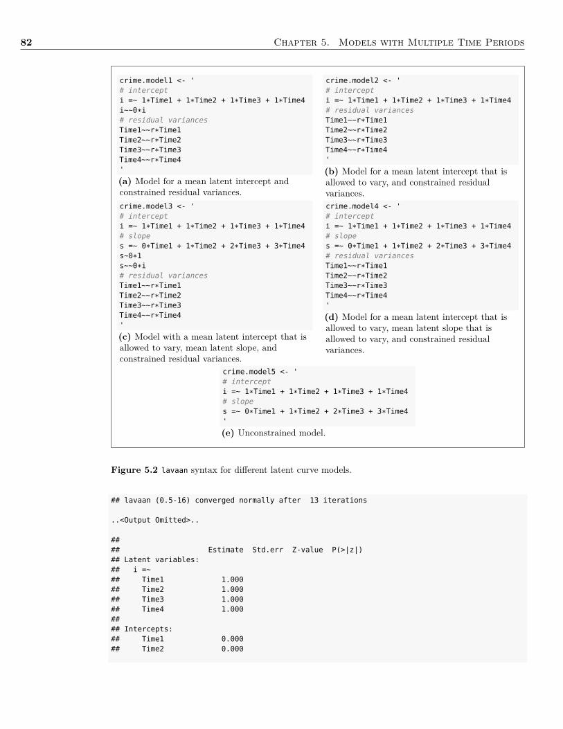
82 Chapter 5. Models with Multiple Time Periods
crime.model1 <- '# intercepti =~ 1*Time1 + 1*Time2 + 1*Time3 + 1*Time4i~~0*i# residual variancesTime1~~r*Time1Time2~~r*Time2Time3~~r*Time3Time4~~r*Time4'
(a) Model for a mean latent intercept andconstrained residual variances.
crime.model2 <- '# intercepti =~ 1*Time1 + 1*Time2 + 1*Time3 + 1*Time4# residual variancesTime1~~r*Time1Time2~~r*Time2Time3~~r*Time3Time4~~r*Time4'
(b) Model for a mean latent intercept that isallowed to vary, and constrained residualvariances.
crime.model3 <- '# intercepti =~ 1*Time1 + 1*Time2 + 1*Time3 + 1*Time4# slopes =~ 0*Time1 + 1*Time2 + 2*Time3 + 3*Time4s~0*1s~~0*i# residual variancesTime1~~r*Time1Time2~~r*Time2Time3~~r*Time3Time4~~r*Time4'
(c) Model with a mean latent intercept that isallowed to vary, mean latent slope, andconstrained residual variances.
crime.model4 <- '# intercepti =~ 1*Time1 + 1*Time2 + 1*Time3 + 1*Time4# slopes =~ 0*Time1 + 1*Time2 + 2*Time3 + 3*Time4# residual variancesTime1~~r*Time1Time2~~r*Time2Time3~~r*Time3Time4~~r*Time4'
(d) Model for a mean latent intercept that isallowed to vary, mean latent slope that isallowed to vary, and constrained residualvariances.
crime.model5 <- '# intercepti =~ 1*Time1 + 1*Time2 + 1*Time3 + 1*Time4# slopes =~ 0*Time1 + 1*Time2 + 2*Time3 + 3*Time4'
(e) Unconstrained model.
Figure 5.2 lavaan syntax for different latent curve models.
## lavaan (0.5-16) converged normally after 13 iterations
..<Output Omitted>..
#### Estimate Std.err Z-value P(>|z|)## Latent variables:## i =~## Time1 1.000## Time2 1.000## Time3 1.000## Time4 1.000#### Intercepts:## Time1 0.000## Time2 0.000

5.2. Example: Latent Curve Model 83
## Time3 0.000## Time4 0.000## i 5.351 0.013 413.817 0.000#### Variances:## i 0.000## Time1 (r) 0.637 0.015## Time2 (r) 0.637 0.015## Time3 (r) 0.637 0.015## Time4 (r) 0.637 0.015
The results show that the mean for the latent intercept, i, is 5.351, indicating that, onaverage, the communities have a crime rate of 5.351 at all time periods. The amount of unex-plained variability (i.e., residual or error variance) is 0.637, indicating that this single-latentintercept model explained 36.327 % of the variability in crime rates.
I do not show the output for the other four LCMs in Figure 5.2 to save space, but in-terpret their results. The second model, crime.model2 (Figure 5.2b), allows the latent inter-cept to vary. Although it still posits there is no change over time, it examines if any of theresidual variance is due to between-community variability. It does this by allowing the latentintercept to have a variance term associated with it. The residual variance for this modelis 0.157, down from 0.637 in the first model. The variance for the latent intercept is 0.48,which, when taken with the knowledge about the residual variance (i.e., within-communityvariability), indicates that 75.4% of the total variance in crime rate is explained by differ-ences between communities.
The third LCM, crime.model3 (Figure 5.2c), allows the latent slope to vary. This modelstill posits there is no systematic change over time, but there are random changes beyondwhat the variability at time one (i.e., latent intercept variance) can explain. With this LCM,the residual variance has now shrunk to 0.11, down from 0.157 in the second model.
The fourth LCM, crime.model4 (Figure 5.2d), finally allows for systematic change in thecrime rate over time as well as variability in this average change, i.e., each county can deviatefrom the average change. In addition, since both the latent intercept and latent slope canvary, this model allows the latent intercept and slope to covary.
The mean for the latent slope, s, is 0.113, indicating that, on average, the crime rate in-creased 0.113 units between each time period. The covariance between the intercept and theslope, -0.023, suggests that there is less crime growth for those communities that had highercrime rates at time point one than for those communities with lower crime rates. The resid-ual variance is now 0.106. While this is substantially lower than the initial estimate of 0.637,within rounding error it is the same as the residual variance in the third model. Moreover,since the the 95% confidence interval for the residual variance (0.10, 0.113) does not contain0.0, this indicates that there is more outcome variance to explain.
The last model, crime.model5 (Figure 5.2e), allows the residual variances to vary acrosstime periods. The unexplained variance for this model ranges from 0.085 to 0.138.
75.4% = 0.480.48+0.157 ×
100
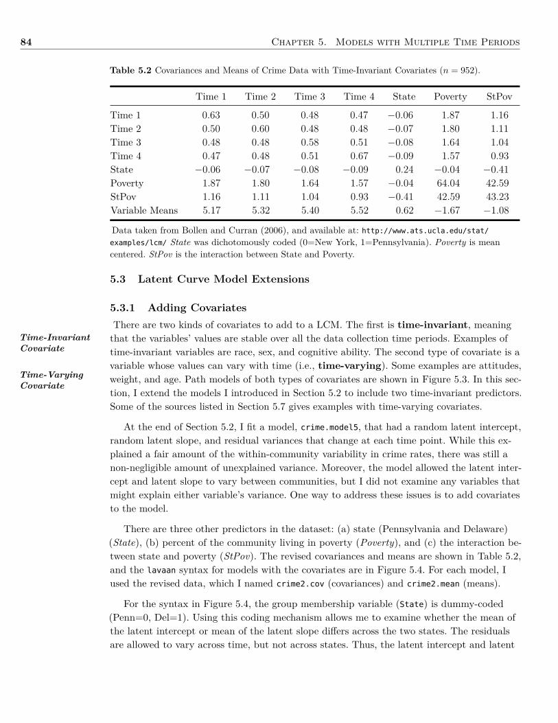
84 Chapter 5. Models with Multiple Time Periods
Table 5.2 Covariances and Means of Crime Data with Time-Invariant Covariates (n = 952).
Time 1 Time 2 Time 3 Time 4 State Poverty StPov
Time 1 0.63 0.50 0.48 0.47 −0.06 1.87 1.16Time 2 0.50 0.60 0.48 0.48 −0.07 1.80 1.11Time 3 0.48 0.48 0.58 0.51 −0.08 1.64 1.04Time 4 0.47 0.48 0.51 0.67 −0.09 1.57 0.93State −0.06 −0.07 −0.08 −0.09 0.24 −0.04 −0.41Poverty 1.87 1.80 1.64 1.57 −0.04 64.04 42.59StPov 1.16 1.11 1.04 0.93 −0.41 42.59 43.23Variable Means 5.17 5.32 5.40 5.52 0.62 −1.67 −1.08
Data taken from Bollen and Curran (2006), and available at: http://www.ats.ucla.edu/stat/examples/lcm/ State was dichotomously coded (0=New York, 1=Pennsylvania). Poverty is meancentered. StPov is the interaction between State and Poverty.
Time-InvariantCovariate
Time-VaryingCovariate
5.3 Latent Curve Model Extensions
5.3.1 Adding CovariatesThere are two kinds of covariates to add to a LCM. The first is time-invariant, meaningthat the variables’ values are stable over all the data collection time periods. Examples oftime-invariant variables are race, sex, and cognitive ability. The second type of covariate is avariable whose values can vary with time (i.e., time-varying). Some examples are attitudes,weight, and age. Path models of both types of covariates are shown in Figure 5.3. In this sec-tion, I extend the models I introduced in Section 5.2 to include two time-invariant predictors.Some of the sources listed in Section 5.7 gives examples with time-varying covariates.
At the end of Section 5.2, I fit a model, crime.model5, that had a random latent intercept,random latent slope, and residual variances that change at each time point. While this ex-plained a fair amount of the within-community variability in crime rates, there was still anon-negligible amount of unexplained variance. Moreover, the model allowed the latent inter-cept and latent slope to vary between communities, but I did not examine any variables thatmight explain either variable’s variance. One way to address these issues is to add covariatesto the model.
There are three other predictors in the dataset: (a) state (Pennsylvania and Delaware)(State), (b) percent of the community living in poverty (Poverty), and (c) the interaction be-tween state and poverty (StPov). The revised covariances and means are shown in Table 5.2,and the lavaan syntax for models with the covariates are in Figure 5.4. For each model, Iused the revised data, which I named crime2.cov (covariances) and crime2.mean (means).
For the syntax in Figure 5.4, the group membership variable (State) is dummy-coded(Penn=0, Del=1). Using this coding mechanism allows me to examine whether the mean ofthe latent intercept or mean of the latent slope differs across the two states. The residualsare allowed to vary across time, but not across states. Thus, the latent intercept and latent
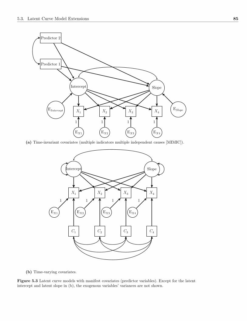
5.3. Latent Curve Model Extensions 85
X3X2X1 X4
EX1 EX2 EX3 EX4
1 1 1 1
Intercept Slope
EIntercept ESlope
Predictor 1
Predictor 2
(a) Time-invariant covariates (multiple indicators multiple independent causes [MIMIC]).
X3X2X1 X4
C1 C2 C3 C4
EX1 EX2 EX3 EX4
1 1 1 1
Intercept Slope
(b) Time-varying covariates.
Figure 5.3 Latent curve models with manifest covariates (predictor variables). Except for the latentintercept and latent slope in (b), the exogenous variables’ variances are not shown.
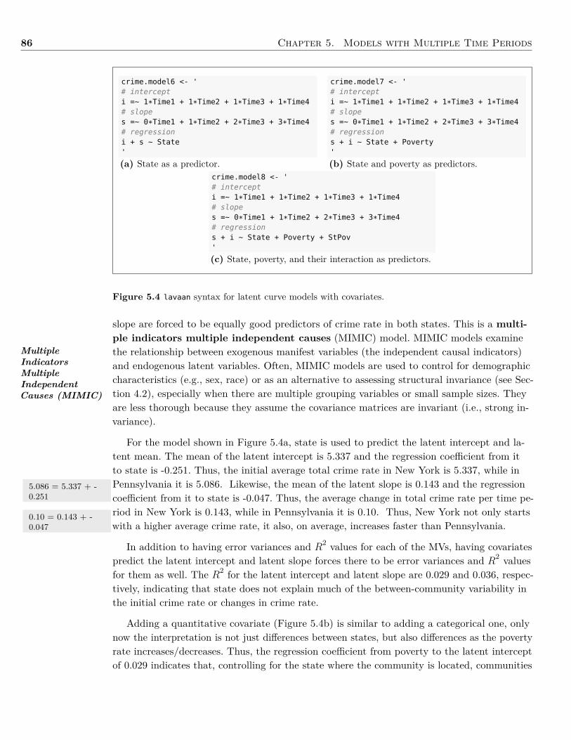
86 Chapter 5. Models with Multiple Time Periods
crime.model6 <- '# intercepti =~ 1*Time1 + 1*Time2 + 1*Time3 + 1*Time4# slopes =~ 0*Time1 + 1*Time2 + 2*Time3 + 3*Time4# regressioni + s ~ State'
(a) State as a predictor.
crime.model7 <- '# intercepti =~ 1*Time1 + 1*Time2 + 1*Time3 + 1*Time4# slopes =~ 0*Time1 + 1*Time2 + 2*Time3 + 3*Time4# regressions + i ~ State + Poverty'
(b) State and poverty as predictors.crime.model8 <- '# intercepti =~ 1*Time1 + 1*Time2 + 1*Time3 + 1*Time4# slopes =~ 0*Time1 + 1*Time2 + 2*Time3 + 3*Time4# regressions + i ~ State + Poverty + StPov'
(c) State, poverty, and their interaction as predictors.
Figure 5.4 lavaan syntax for latent curve models with covariates.
MultipleIndicatorsMultipleIndependentCauses (MIMIC)
5.086 = 5.337 + -0.251
0.10 = 0.143 + -0.047
slope are forced to be equally good predictors of crime rate in both states. This is a multi-ple indicators multiple independent causes (MIMIC) model. MIMIC models examinethe relationship between exogenous manifest variables (the independent causal indicators)and endogenous latent variables. Often, MIMIC models are used to control for demographiccharacteristics (e.g., sex, race) or as an alternative to assessing structural invariance (see Sec-tion 4.2), especially when there are multiple grouping variables or small sample sizes. Theyare less thorough because they assume the covariance matrices are invariant (i.e., strong in-variance).
For the model shown in Figure 5.4a, state is used to predict the latent intercept and la-tent mean. The mean of the latent intercept is 5.337 and the regression coefficient from itto state is -0.251. Thus, the initial average total crime rate in New York is 5.337, while inPennsylvania it is 5.086. Likewise, the mean of the latent slope is 0.143 and the regressioncoefficient from it to state is -0.047. Thus, the average change in total crime rate per time pe-riod in New York is 0.143, while in Pennsylvania it is 0.10. Thus, New York not only startswith a higher average crime rate, it also, on average, increases faster than Pennsylvania.
In addition to having error variances and R2 values for each of the MVs, having covariatespredict the latent intercept and latent slope forces there to be error variances and R2 valuesfor them as well. The R2 for the latent intercept and latent slope are 0.029 and 0.036, respec-tively, indicating that state does not explain much of the between-community variability inthe initial crime rate or changes in crime rate.
Adding a quantitative covariate (Figure 5.4b) is similar to adding a categorical one, onlynow the interpretation is not just differences between states, but also differences as the povertyrate increases/decreases. Thus, the regression coefficient from poverty to the latent interceptof 0.029 indicates that, controlling for the state where the community is located, communities
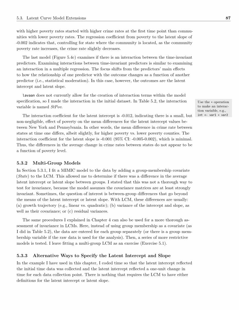
5.3. Latent Curve Model Extensions 87
with higher poverty rates started with higher crime rates at the first time point than commu-nities with lower poverty rates. The regression coefficient from poverty to the latent slope of-0.002 indicates that, controlling for state where the community is located, as the communitypoverty rate increases, the crime rate slightly decreases.
The last model (Figure 5.4c) examines if there is an interaction between the time-invariantpredictors. Examining interactions between time-invariant predictors is similar to examiningan interaction in a multiple regression. The focus shifts from the predictors’ main effectsto how the relationship of one predictor with the outcome changes as a function of anotherpredictor (i.e., statistical moderation). In this case, however, the outcomes are the latentintercept and latent slope.
lavaan does not currently allow for the creation of interaction terms within the modelspecification, so I made the interaction in the initial dataset. In Table 5.2, the interactionvariable is named StPov.
The interaction coefficient for the latent intercept is -0.012, indicating there is a small, butnon-negligible, effect of poverty on the mean differences for the latent intercept values be-tween New York and Pennsylvania. In other words, the mean difference in crime rate betweenstates at time one differs, albeit slightly, for higher poverty vs. lower poverty counties. Theinteraction coefficient for the latent slope is -0.001 (95% CI: -0.005-0.002), which is minimal.Thus, the differences in the average change in crime rates between states do not appear to bea function of poverty level.
5.3.2 Multi-Group ModelsIn Section 5.3.1, I fit a MIMIC model to the data by adding a group-membership covariate(State) to the LCM. This allowed me to determine if there was a difference in the averagelatent intercept or latent slope between groups. I stated that this was not a thorough way totest for invariance, because the model assumes the covariance matrices are at least stronglyinvariant. Sometimes, the question of interest is between-group differences that go beyondthe means of the latent intercept or latent slope. With LCM, these differences are usually:(a) growth trajectory (e.g., linear vs. quadratic); (b) variance of the intercept and slope, aswell as their covariance; or (c) residual variances.
The same procedures I explained in Chapter 4 can also be used for a more thorough as-sessment of invariance in LCMs. Here, instead of using group membership as a covariate (asI did in Table 5.2), the data are entered for each group separately (or there is a group mem-bership variable if the raw data is used for the analysis). Then, a series of more restrictivemodels is tested. I leave fitting a multi-group LCM as an exercise (Exercise 5.1).
5.3.3 Alternative Ways to Specify the Latent Intercept and SlopeIn the example I have used in this chapter, I coded time so that the latent intercept reflectedthe initial time data was collected and the latent intercept reflected a one-unit change intime for each data collection point. There is nothing that requires the LCM to have eitherdefinitions for the latent intercept or latent slope.
Use the * operationto make an interac-tion variable, e.g.,int <- var1 * var2
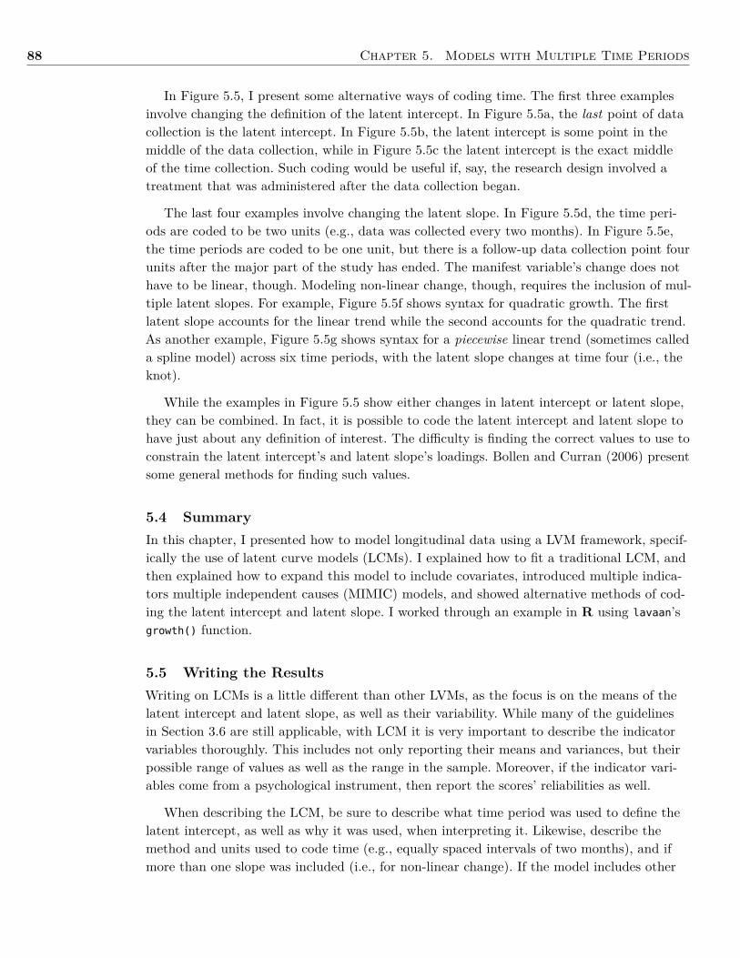
88 Chapter 5. Models with Multiple Time Periods
In Figure 5.5, I present some alternative ways of coding time. The first three examplesinvolve changing the definition of the latent intercept. In Figure 5.5a, the last point of datacollection is the latent intercept. In Figure 5.5b, the latent intercept is some point in themiddle of the data collection, while in Figure 5.5c the latent intercept is the exact middleof the time collection. Such coding would be useful if, say, the research design involved atreatment that was administered after the data collection began.
The last four examples involve changing the latent slope. In Figure 5.5d, the time peri-ods are coded to be two units (e.g., data was collected every two months). In Figure 5.5e,the time periods are coded to be one unit, but there is a follow-up data collection point fourunits after the major part of the study has ended. The manifest variable’s change does nothave to be linear, though. Modeling non-linear change, though, requires the inclusion of mul-tiple latent slopes. For example, Figure 5.5f shows syntax for quadratic growth. The firstlatent slope accounts for the linear trend while the second accounts for the quadratic trend.As another example, Figure 5.5g shows syntax for a piecewise linear trend (sometimes calleda spline model) across six time periods, with the latent slope changes at time four (i.e., theknot).
While the examples in Figure 5.5 show either changes in latent intercept or latent slope,they can be combined. In fact, it is possible to code the latent intercept and latent slope tohave just about any definition of interest. The difficulty is finding the correct values to use toconstrain the latent intercept’s and latent slope’s loadings. Bollen and Curran (2006) presentsome general methods for finding such values.
5.4 SummaryIn this chapter, I presented how to model longitudinal data using a LVM framework, specif-ically the use of latent curve models (LCMs). I explained how to fit a traditional LCM, andthen explained how to expand this model to include covariates, introduced multiple indica-tors multiple independent causes (MIMIC) models, and showed alternative methods of cod-ing the latent intercept and latent slope. I worked through an example in R using lavaan’sgrowth() function.
5.5 Writing the ResultsWriting on LCMs is a little different than other LVMs, as the focus is on the means of thelatent intercept and latent slope, as well as their variability. While many of the guidelinesin Section 3.6 are still applicable, with LCM it is very important to describe the indicatorvariables thoroughly. This includes not only reporting their means and variances, but theirpossible range of values as well as the range in the sample. Moreover, if the indicator vari-ables come from a psychological instrument, then report the scores’ reliabilities as well.
When describing the LCM, be sure to describe what time period was used to define thelatent intercept, as well as why it was used, when interpreting it. Likewise, describe themethod and units used to code time (e.g., equally spaced intervals of two months), and ifmore than one slope was included (i.e., for non-linear change). If the model includes other
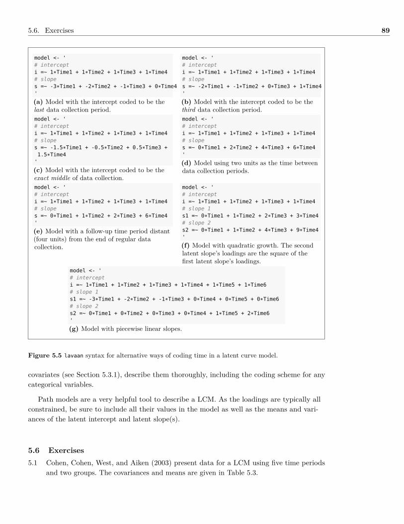
5.6. Exercises 89
model <- '# intercepti =~ 1*Time1 + 1*Time2 + 1*Time3 + 1*Time4# slopes =~ -3*Time1 + -2*Time2 + -1*Time3 + 0*Time4'
(a) Model with the intercept coded to be thelast data collection period.
model <- '# intercepti =~ 1*Time1 + 1*Time2 + 1*Time3 + 1*Time4# slopes =~ -2*Time1 + -1*Time2 + 0*Time3 + 1*Time4'
(b) Model with the intercept coded to be thethird data collection period.
model <- '# intercepti =~ 1*Time1 + 1*Time2 + 1*Time3 + 1*Time4# slopes =~ -1.5*Time1 + -0.5*Time2 + 0.5*Time3 +1.5*Time4
'
(c) Model with the intercept coded to be theexact middle of data collection.
model <- '# intercepti =~ 1*Time1 + 1*Time2 + 1*Time3 + 1*Time4# slopes =~ 0*Time1 + 2*Time2 + 4*Time3 + 6*Time4'
(d) Model using two units as the time betweendata collection periods.
model <- '# intercepti =~ 1*Time1 + 1*Time2 + 1*Time3 + 1*Time4# slopes =~ 0*Time1 + 1*Time2 + 2*Time3 + 6*Time4'
(e) Model with a follow-up time period distant(four units) from the end of regular datacollection.
model <- '# intercepti =~ 1*Time1 + 1*Time2 + 1*Time3 + 1*Time4# slope 1s1 =~ 0*Time1 + 1*Time2 + 2*Time3 + 3*Time4# slope 2s2 =~ 0*Time1 + 1*Time2 + 4*Time3 + 9*Time4'
(f) Model with quadratic growth. The secondlatent slope’s loadings are the square of thefirst latent slope’s loadings.
model <- '# intercepti =~ 1*Time1 + 1*Time2 + 1*Time3 + 1*Time4 + 1*Time5 + 1*Time6# slope 1s1 =~ -3*Time1 + -2*Time2 + -1*Time3 + 0*Time4 + 0*Time5 + 0*Time6# slope 2s2 =~ 0*Time1 + 0*Time2 + 0*Time3 + 0*Time4 + 1*Time5 + 2*Time6'
(g) Model with piecewise linear slopes.
Figure 5.5 lavaan syntax for alternative ways of coding time in a latent curve model.
covariates (see Section 5.3.1), describe them thoroughly, including the coding scheme for anycategorical variables.
Path models are a very helpful tool to describe a LCM. As the loadings are typically allconstrained, be sure to include all their values in the model as well as the means and vari-ances of the latent intercept and latent slope(s).
5.6 Exercises5.1 Cohen, Cohen, West, and Aiken (2003) present data for a LCM using five time periods
and two groups. The covariances and means are given in Table 5.3.
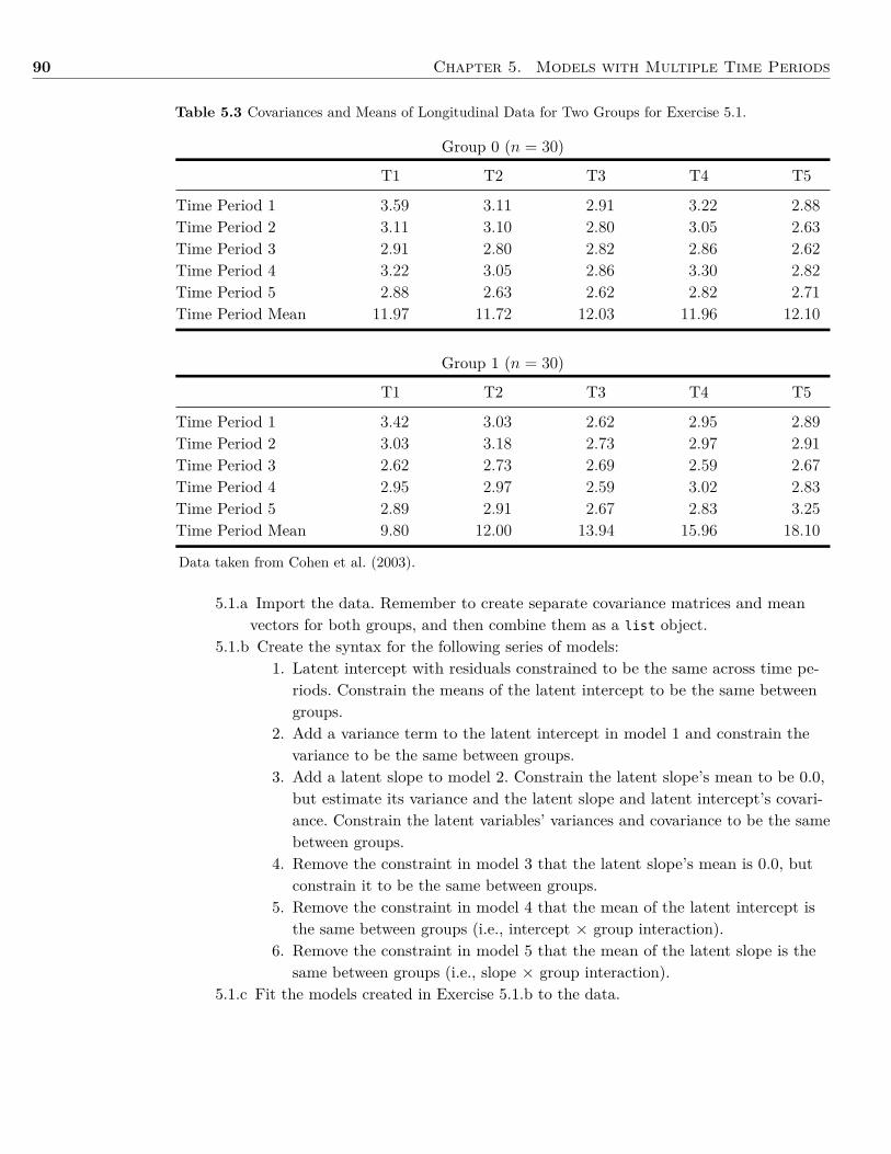
90 Chapter 5. Models with Multiple Time Periods
Table 5.3 Covariances and Means of Longitudinal Data for Two Groups for Exercise 5.1.
Group 0 (n = 30)
T1 T2 T3 T4 T5
Time Period 1 3.59 3.11 2.91 3.22 2.88Time Period 2 3.11 3.10 2.80 3.05 2.63Time Period 3 2.91 2.80 2.82 2.86 2.62Time Period 4 3.22 3.05 2.86 3.30 2.82Time Period 5 2.88 2.63 2.62 2.82 2.71Time Period Mean 11.97 11.72 12.03 11.96 12.10
Group 1 (n = 30)
T1 T2 T3 T4 T5
Time Period 1 3.42 3.03 2.62 2.95 2.89Time Period 2 3.03 3.18 2.73 2.97 2.91Time Period 3 2.62 2.73 2.69 2.59 2.67Time Period 4 2.95 2.97 2.59 3.02 2.83Time Period 5 2.89 2.91 2.67 2.83 3.25Time Period Mean 9.80 12.00 13.94 15.96 18.10
Data taken from Cohen et al. (2003).
5.1.a Import the data. Remember to create separate covariance matrices and meanvectors for both groups, and then combine them as a list object.
5.1.b Create the syntax for the following series of models:1. Latent intercept with residuals constrained to be the same across time pe-
riods. Constrain the means of the latent intercept to be the same betweengroups.
2. Add a variance term to the latent intercept in model 1 and constrain thevariance to be the same between groups.
3. Add a latent slope to model 2. Constrain the latent slope’s mean to be 0.0,but estimate its variance and the latent slope and latent intercept’s covari-ance. Constrain the latent variables’ variances and covariance to be the samebetween groups.
4. Remove the constraint in model 3 that the latent slope’s mean is 0.0, butconstrain it to be the same between groups.
5. Remove the constraint in model 4 that the mean of the latent intercept isthe same between groups (i.e., intercept × group interaction).
6. Remove the constraint in model 5 that the mean of the latent slope is thesame between groups (i.e., slope × group interaction).
5.1.c Fit the models created in Exercise 5.1.b to the data.
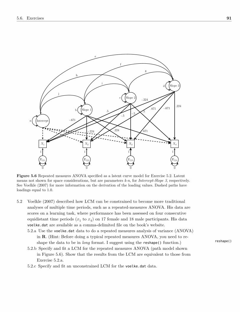
5.6. Exercises 91
X3X2X1 X4
EX1 EX2 EX3 EX4
1 1 1 1
0 0 0 0
Intercept
Slope 1
Slope 2
Slope 3
-.224 .224 .671
-.671-.5
-.5 .5.5.671 -.671
.224
-.224
a
b
c
d
e
f
gh
i
j
Figure 5.6 Repeated measures ANOVA specified as a latent curve model for Exercise 5.2. Latentmeans not shown for space considerations, but are parameters k-n, for Intercept-Slope 3, respectively.See Voelkle (2007) for more information on the derivation of the loading values. Dashed paths haveloadings equal to 1.0.
5.2 Voelkle (2007) described how LCM can be constrained to become more traditionalanalyses of multiple time periods, such as a repeated-measures ANOVA. His data arescores on a learning task, where performance has been assessed on four consecutiveequidistant time periods (x1 to x4) on 17 female and 18 male participants. His datavoelke.dat are available as a comma-delimited file on the book’s website.5.2.a Use the voelke.dat data to do a repeated measures analysis of variance (ANOVA)
in R. (Hint: Before doing a typical repeated measures ANOVA, you need to re-shape the data to be in long format. I suggest using the reshape() function.)
5.2.b Specify and fit a LCM for the repeated measures ANOVA (path model shownin Figure 5.6). Show that the results from the LCM are equivalent to those fromExercise 5.2.a.
5.2.c Specify and fit an unconstrained LCM for the voelke.dat data.
reshape()
92 Chapter 5. Models with Multiple Time Periods
5.7 References & Further ReadingsAiken, L. S., & West, S. G. (1991). Multiple regression: Testing and interpreting interactions.
Newbury Park, CA: Sage.Bollen, K. A., & Curran, P. J. (2006). Latent curve models: A structural equation perspective.
Hoboken, NJ: Wiley.Cohen, J., Cohen, P., West, S. G., & Aiken, L. S. (2003). Applied multiple
regression/correlation analysis for the behavioral sciences (3rd ed.). Mahwah, NJ:Lawrence Erlbaum.
Muthén, B. O. (1989). Latent variable modeling in heterogeneous populations. Psychometrika,54 , 557-585. doi: 10.1007/BF02296397
Muthén, B. O., & Curran, P. J. (1997). General longitudinal modeling of individual differencesin experimental designs: A latent variable framework for analysis and power estimation.Psychological Methods, 2 , 371-402. doi: 10.1037/1082-989X.2.4.371
Preacher, K. J., Wichman, A. L., MacCallum, R. C., & Briggs, N. E. (2008). Latent growthcurve modeling. Thousand Oaks, CA: Sage.
Voelkle, M. C. (2007). Latent growth curve modeling as an integrative approach to theanalysis of change. Psychology Science, 49 , 375-414.
6 | Models with DichotomousIndicator Variables
Chapter Contents6.1 Background . . . . . . . . . . . . . . . . . . . . . . . . . . . . . . . . . . . . 93
6.1.1 Item Factor Analysis . . . . . . . . . . . . . . . . . . . . . . . . . . . 966.1.2 Parameterizing the Model . . . . . . . . . . . . . . . . . . . . . . . . 996.1.3 Item Response Theory . . . . . . . . . . . . . . . . . . . . . . . . . . 1006.1.4 Relationship Between Item Response and Factor Analysis Models . . 104
6.2 Example: Dichotomous Indicator Variables . . . . . . . . . . . . . . . . . . . 1046.2.1 Item Response Theory Parameter Estimation . . . . . . . . . . . . . 1056.2.2 Item Factor Analysis Parameter Estimation . . . . . . . . . . . . . . 107
6.3 Summary . . . . . . . . . . . . . . . . . . . . . . . . . . . . . . . . . . . . . . 1096.4 Writing the Results . . . . . . . . . . . . . . . . . . . . . . . . . . . . . . . . 1106.5 Exercises . . . . . . . . . . . . . . . . . . . . . . . . . . . . . . . . . . . . . . 1116.6 References & Further Readings . . . . . . . . . . . . . . . . . . . . . . . . . . 112
6.1 BackgroundThus far, the only LVMs I have covered have assumed that the indicator variables were con-tinuous. When the indicators are categorical, the LVM needs some modification to accountfor the fact that the outcomes can only attain a small, finite number of values. If adjustmentsare not made and, instead, the parameters are estimated under the assumption that the indi-cator variables are continuous, the estimated covariances for the indicator variables tend tobe spuriously high. If the number of possible response categories is > 4 and the distributionof the responses approximately follows a normal distribution (i.e., symmetrical with moreresponses in the middle than the extremes), then treating the data as being continuous willtypically not substantially alter the parameter estimates, a robust estimator should be used(see Section A.1.1.1). Consequently, this chapter only deals with the most extreme case ofcategorical variables: those with only two response options–otherwise known as dichotomousvariables.
Traditionally, LVMs with categorical outcomes were used for item-level analyses of psy-chometric instruments (e.g., extraversion scale, test of math knowledge), so they assumedthat the indicator variables were unidimensional (i.e., only measure one LV) and locally in-dependent. Multidimensional (i.e, more than one LV) models with dichotomous items arebecoming more well-developed and used, but are beyond the scope of this chapter. Some ofthe references in Section 6.5 give more information about multidimensional models. Localindependence is a complex topic. The gist of the assumption is that after controlling for dif-ferences in the LV, the items are unrelated to each other (i.e., no correlated errors).
When discussingdichotomous indica-tor variables, I usethe terms item andindicator variableinterchangeably.
93
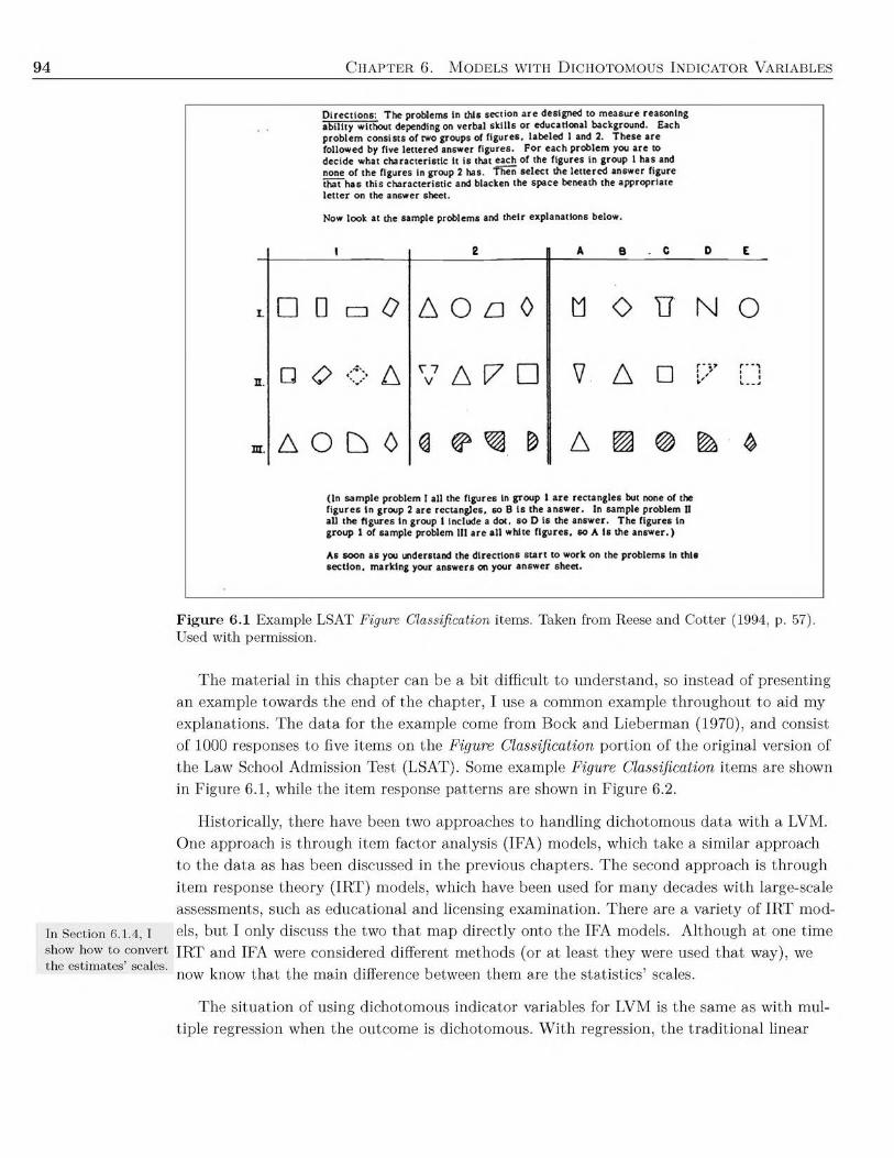
94 C h a p t e r 6 . M o d e l s w i t h D i c h o t o m o u s I n d i c a t o r V a r i a b l e s
D irec tio n s : T he problem s In this section a re designed to m easu re reasoning ab ility without depending on verbal s k ills o r educational background. Each p ro b lem c o n sis ts of two groups of f ig u res , labe led 1 and 2. T h ese a re followed by five le ttered answ er figures. F o r each p roblem you a re to decide what ch a rac te ris tic It is that each of the figu res in group 1 has and none of th e figures in group 2 has. Then se lec t the le tte re d answ er figure that h a s th is ch a rac te ris tic and blacken the space beneath the app rop ria te le t te r on the answ er sheet.
Now look at the sam ple problem s and th e ir explanations below.
(In sam p le problem 1 all the figures In g roup t a re rec tan g les but none of the fig u res In group 2 a re rec tang les , so 6 is the an sw er. In sam ple problem II all the fig u res In group I Include a dot, so D is the answ er. T h e figures In group 1 of sam ple problem III a re all white fig u res , so A Is the an sw er.)
As soon a s you understand the d irec tions s ta r t to work on the p rob lem s In th is s ec tio n , m arking your answ ers on your answ er sheet.
In Section 6.1.4, I show how to convert the estim ates’ scales.
Figure 6.1 Example LSAT Figure Classification items. Taken from Reese and Cotter (1994, p. 57). Used with permission.
The material in this chapter can be a bit difficult to understand, so instead of presenting an example towards the end of the chapter, I use a common example throughout to aid my explanations. The data for the example come from Bock and Lieberman (1970), and consist of 1000 responses to five items on the Figure Classification portion of the original version of the Law School Admission Test (LSAT). Some example Figure Classification items are shown in Figure 6.1, while the item response patterns are shown in Figure 6.2.
Historically, there have been two approaches to handling dichotomous data with a LVM. One approach is through item factor analysis (IFA) models, which take a similar approach to the data as has been discussed in the previous chapters. The second approach is through item response theory (IRT) models, which have been used for many decades with large-scale assessments, such as educational and licensing examination. There are a variety of IRT models, but I only discuss the two tha t map directly onto the IFA models. Although at one time IRT and IFA were considered different methods (or at least they were used tha t way), we now know tha t the main difference between them are the statistics’ scales.
The situation of using dichotomous indicator variables for LVM is the same as with multiple regression when the outcome is dichotomous. W ith regression, the traditional linear
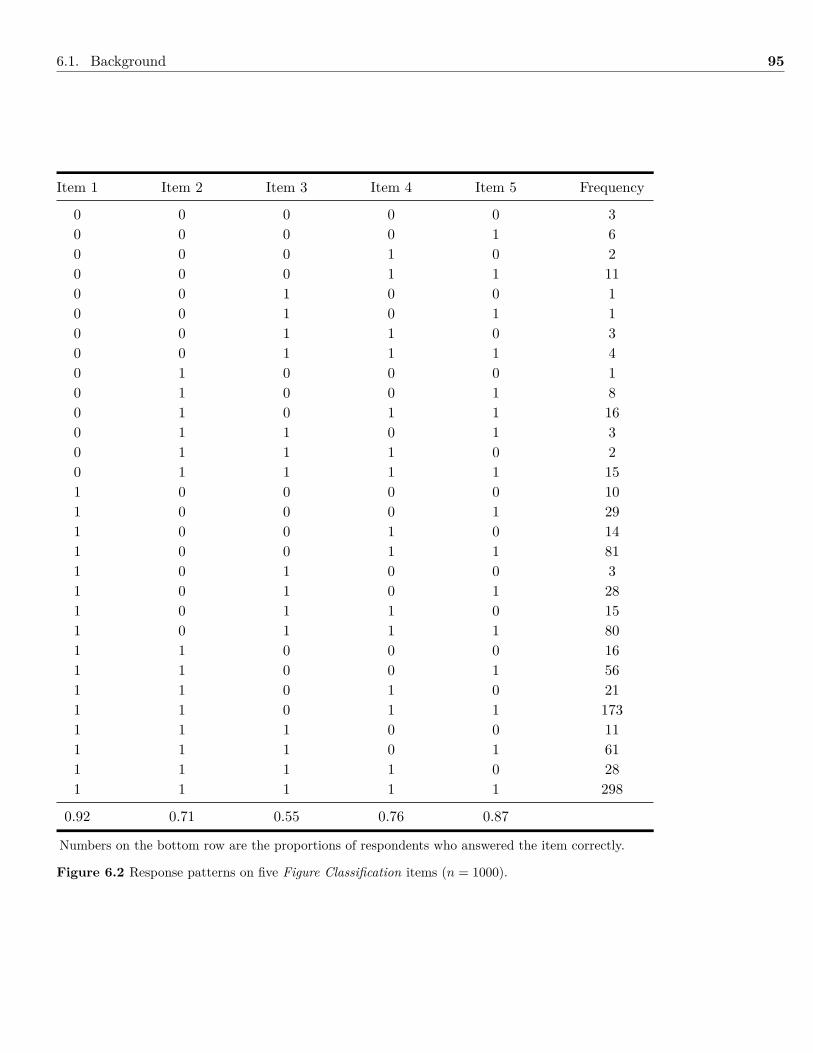
6.1. Background 95
Item 1 Item 2 Item 3 Item 4 Item 5 Frequency
0 0 0 0 0 30 0 0 0 1 60 0 0 1 0 20 0 0 1 1 110 0 1 0 0 10 0 1 0 1 10 0 1 1 0 30 0 1 1 1 40 1 0 0 0 10 1 0 0 1 80 1 0 1 1 160 1 1 0 1 30 1 1 1 0 20 1 1 1 1 151 0 0 0 0 101 0 0 0 1 291 0 0 1 0 141 0 0 1 1 811 0 1 0 0 31 0 1 0 1 281 0 1 1 0 151 0 1 1 1 801 1 0 0 0 161 1 0 0 1 561 1 0 1 0 211 1 0 1 1 1731 1 1 0 0 111 1 1 0 1 611 1 1 1 0 281 1 1 1 1 298
0.92 0.71 0.55 0.76 0.87
Numbers on the bottom row are the proportions of respondents who answered the item correctly.
Figure 6.2 Response patterns on five Figure Classification items (n = 1000).
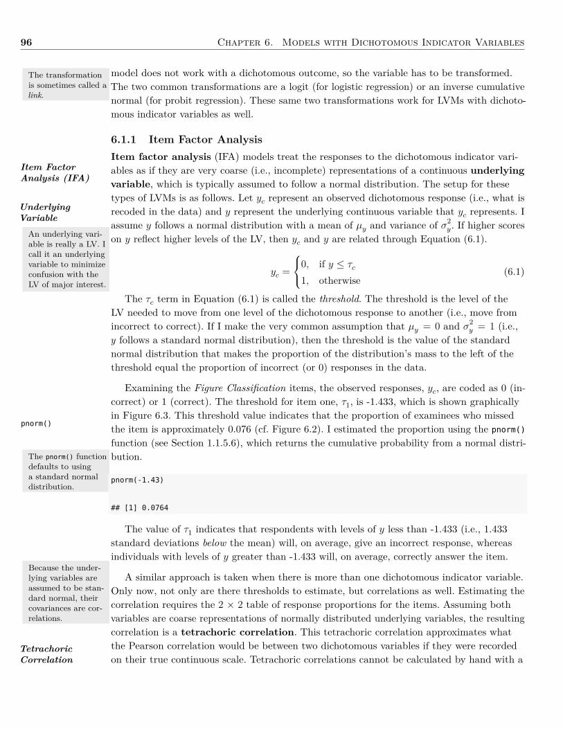
96 Chapter 6. Models with Dichotomous Indicator Variables
The transformationis sometimes called alink.
Item FactorAnalysis (IFA)
UnderlyingVariable
An underlying vari-able is really a LV. Icall it an underlyingvariable to minimizeconfusion with theLV of major interest.
pnorm()
The pnorm() functiondefaults to usinga standard normaldistribution.
Because the under-lying variables areassumed to be stan-dard normal, theircovariances are cor-relations.
TetrachoricCorrelation
model does not work with a dichotomous outcome, so the variable has to be transformed.The two common transformations are a logit (for logistic regression) or an inverse cumulativenormal (for probit regression). These same two transformations work for LVMs with dichoto-mous indicator variables as well.
6.1.1 Item Factor AnalysisItem factor analysis (IFA) models treat the responses to the dichotomous indicator vari-ables as if they are very coarse (i.e., incomplete) representations of a continuous underlyingvariable, which is typically assumed to follow a normal distribution. The setup for thesetypes of LVMs is as follows. Let yc represent an observed dichotomous response (i.e., what isrecoded in the data) and y represent the underlying continuous variable that yc represents. Iassume y follows a normal distribution with a mean of µy and variance of σ2
y. If higher scoreson y reflect higher levels of the LV, then yc and y are related through Equation (6.1).
yc =
0, if y ≤ τc
1, otherwise(6.1)
The τc term in Equation (6.1) is called the threshold. The threshold is the level of theLV needed to move from one level of the dichotomous response to another (i.e., move fromincorrect to correct). If I make the very common assumption that µy = 0 and σ2
y = 1 (i.e.,y follows a standard normal distribution), then the threshold is the value of the standardnormal distribution that makes the proportion of the distribution’s mass to the left of thethreshold equal the proportion of incorrect (or 0) responses in the data.
Examining the Figure Classification items, the observed responses, yc, are coded as 0 (in-correct) or 1 (correct). The threshold for item one, τ1, is -1.433, which is shown graphicallyin Figure 6.3. This threshold value indicates that the proportion of examinees who missedthe item is approximately 0.076 (cf. Figure 6.2). I estimated the proportion using the pnorm()
function (see Section 1.1.5.6), which returns the cumulative probability from a normal distri-bution.
pnorm(-1.43)
## [1] 0.0764
The value of τ1 indicates that respondents with levels of y less than -1.433 (i.e., 1.433standard deviations below the mean) will, on average, give an incorrect response, whereasindividuals with levels of y greater than -1.433 will, on average, correctly answer the item.
A similar approach is taken when there is more than one dichotomous indicator variable.Only now, not only are there thresholds to estimate, but correlations as well. Estimating thecorrelation requires the 2 × 2 table of response proportions for the items. Assuming bothvariables are coarse representations of normally distributed underlying variables, the resultingcorrelation is a tetrachoric correlation. This tetrachoric correlation approximates whatthe Pearson correlation would be between two dichotomous variables if they were recordedon their true continuous scale. Tetrachoric correlations cannot be calculated by hand with a
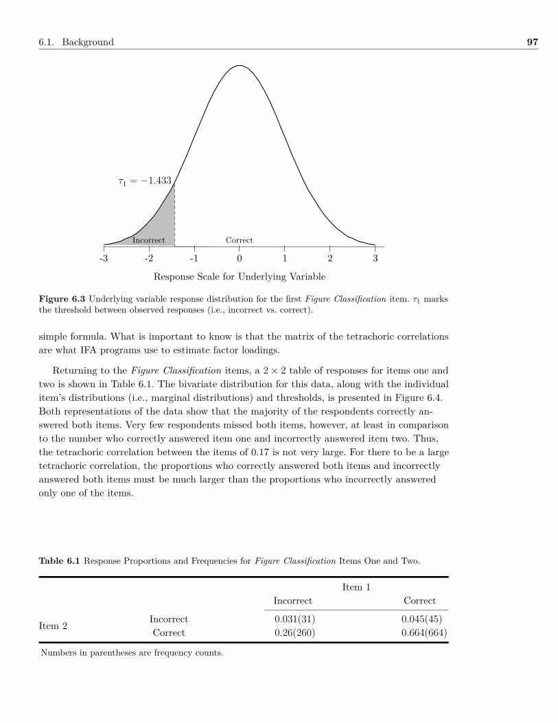
6.1. Background 97
τ1 = −1.433
Response Scale for Underlying Variable
-3 -2 -1 0 1 2 3
CorrectIncorrect
Figure 6.3 Underlying variable response distribution for the first Figure Classification item. τ1 marksthe threshold between observed responses (i.e., incorrect vs. correct).
simple formula. What is important to know is that the matrix of the tetrachoric correlationsare what IFA programs use to estimate factor loadings.
Returning to the Figure Classification items, a 2× 2 table of responses for items one andtwo is shown in Table 6.1. The bivariate distribution for this data, along with the individualitem’s distributions (i.e., marginal distributions) and thresholds, is presented in Figure 6.4.Both representations of the data show that the majority of the respondents correctly an-swered both items. Very few respondents missed both items, however, at least in comparisonto the number who correctly answered item one and incorrectly answered item two. Thus,the tetrachoric correlation between the items of 0.17 is not very large. For there to be a largetetrachoric correlation, the proportions who correctly answered both items and incorrectlyanswered both items must be much larger than the proportions who incorrectly answeredonly one of the items.
Table 6.1 Response Proportions and Frequencies for Figure Classification Items One and Two.
Item 1Incorrect Correct
Item 2 Incorrect 0.031(31) 0.045(45)Correct 0.26(260) 0.664(664)
Numbers in parentheses are frequency counts.
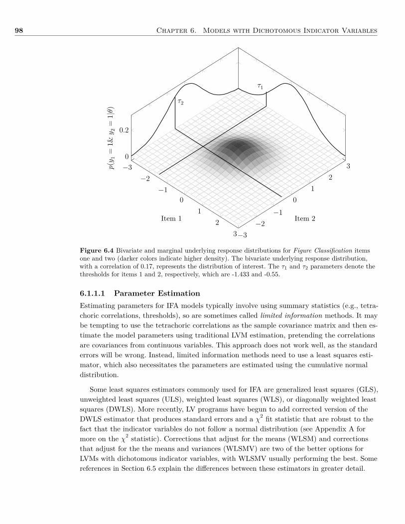
98 Chapter 6. Models with Dichotomous Indicator Variables
−3−2
−10
12
3−3−2
−10
12
30
0.2
τ1
τ2
Item 1 Item 2
p(y 1
=1&
y 2=
1|θ)
Figure 6.4 Bivariate and marginal underlying response distributions for Figure Classification itemsone and two (darker colors indicate higher density). The bivariate underlying response distribution,with a correlation of 0.17, represents the distribution of interest. The τ1 and τ2 parameters denote thethresholds for items 1 and 2, respectively, which are -1.433 and -0.55.
6.1.1.1 Parameter EstimationEstimating parameters for IFA models typically involve using summary statistics (e.g., tetra-choric correlations, thresholds), so are sometimes called limited information methods. It maybe tempting to use the tetrachoric correlations as the sample covariance matrix and then es-timate the model parameters using traditional LVM estimation, pretending the correlationsare covariances from continuous variables. This approach does not work well, as the standarderrors will be wrong. Instead, limited information methods need to use a least squares esti-mator, which also necessitates the parameters are estimated using the cumulative normaldistribution.
Some least squares estimators commonly used for IFA are generalized least squares (GLS),unweighted least squares (ULS), weighted least squares (WLS), or diagonally weighted leastsquares (DWLS). More recently, LV programs have begun to add corrected version of theDWLS estimator that produces standard errors and a χ2 fit statistic that are robust to thefact that the indicator variables do not follow a normal distribution (see Appendix A formore on the χ2 statistic). Corrections that adjust for the means (WLSM) and correctionsthat adjust for the the means and variances (WLSMV) are two of the better options forLVMs with dichotomous indicator variables, with WLSMV usually performing the best. Somereferences in Section 6.5 explain the differences between these estimators in greater detail.
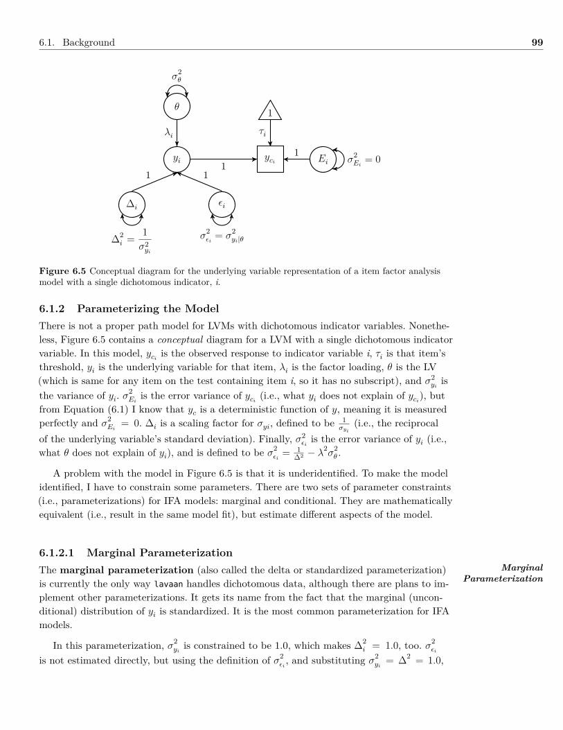
6.1. Background 99
θ
yi
εi∆i
yci
1
Ei
σ2εi
= σ2yi|θ∆2
i = 1σ2yi
σ2θ
σ2Ei
= 011
τiλi
11
Figure 6.5 Conceptual diagram for the underlying variable representation of a item factor analysismodel with a single dichotomous indicator, i.
6.1.2 Parameterizing the ModelThere is not a proper path model for LVMs with dichotomous indicator variables. Nonethe-less, Figure 6.5 contains a conceptual diagram for a LVM with a single dichotomous indicatorvariable. In this model, yci
is the observed response to indicator variable i, τi is that item’sthreshold, yi is the underlying variable for that item, λi is the factor loading, θ is the LV(which is same for any item on the test containing item i, so it has no subscript), and σ2
yiis
the variance of yi. σ2Ei
is the error variance of yci(i.e., what yi does not explain of yci
), butfrom Equation (6.1) I know that yc is a deterministic function of y, meaning it is measuredperfectly and σ2
Ei= 0. ∆i is a scaling factor for σyi, defined to be 1
σyi(i.e., the reciprocal
of the underlying variable’s standard deviation). Finally, σ2εiis the error variance of yi (i.e.,
what θ does not explain of yi), and is defined to be σ2εi
= 1∆2 − λ2
σ2θ .
A problem with the model in Figure 6.5 is that it is underidentified. To make the modelidentified, I have to constrain some parameters. There are two sets of parameter constraints(i.e., parameterizations) for IFA models: marginal and conditional. They are mathematicallyequivalent (i.e., result in the same model fit), but estimate different aspects of the model.
6.1.2.1 Marginal ParameterizationThe marginal parameterization (also called the delta or standardized parameterization)is currently the only way lavaan handles dichotomous data, although there are plans to im-plement other parameterizations. It gets its name from the fact that the marginal (uncon-ditional) distribution of yi is standardized. It is the most common parameterization for IFAmodels.
In this parameterization, σ2yi
is constrained to be 1.0, which makes ∆2i = 1.0, too. σ2
εi
is not estimated directly, but using the definition of σ2εi, and substituting σ2
yi= ∆2 = 1.0,
MarginalParameterization
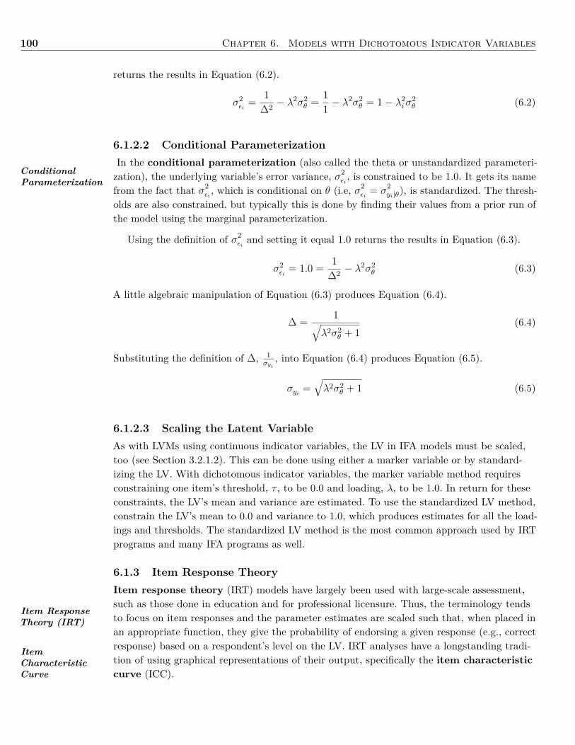
100 Chapter 6. Models with Dichotomous Indicator Variables
ConditionalParameterization
Item ResponseTheory (IRT)
ItemCharacteristicCurve
returns the results in Equation (6.2).
σ2εi
= 1∆2 − λ
2σ2θ = 1
1 − λ2σ2
θ = 1− λ2iσ
2θ (6.2)
6.1.2.2 Conditional ParameterizationIn the conditional parameterization (also called the theta or unstandardized parameteri-zation), the underlying variable’s error variance, σ2
εi, is constrained to be 1.0. It gets its name
from the fact that σ2εi, which is conditional on θ (i.e, σ2
εi= σ
2yi|θ), is standardized. The thresh-
olds are also constrained, but typically this is done by finding their values from a prior run ofthe model using the marginal parameterization.
Using the definition of σ2εiand setting it equal 1.0 returns the results in Equation (6.3).
σ2εi
= 1.0 = 1∆2 − λ
2σ2θ (6.3)
A little algebraic manipulation of Equation (6.3) produces Equation (6.4).
∆ = 1√λ2σ2
θ + 1(6.4)
Substituting the definition of ∆, 1σyi
, into Equation (6.4) produces Equation (6.5).
σyi=√λ2σ2
θ + 1 (6.5)
6.1.2.3 Scaling the Latent VariableAs with LVMs using continuous indicator variables, the LV in IFA models must be scaled,too (see Section 3.2.1.2). This can be done using either a marker variable or by standard-izing the LV. With dichotomous indicator variables, the marker variable method requiresconstraining one item’s threshold, τ , to be 0.0 and loading, λ, to be 1.0. In return for theseconstraints, the LV’s mean and variance are estimated. To use the standardized LV method,constrain the LV’s mean to 0.0 and variance to 1.0, which produces estimates for all the load-ings and thresholds. The standardized LV method is the most common approach used by IRTprograms and many IFA programs as well.
6.1.3 Item Response TheoryItem response theory (IRT) models have largely been used with large-scale assessment,such as those done in education and for professional licensure. Thus, the terminology tendsto focus on item responses and the parameter estimates are scaled such that, when placed inan appropriate function, they give the probability of endorsing a given response (e.g., correctresponse) based on a respondent’s level on the LV. IRT analyses have a longstanding tradi-tion of using graphical representations of their output, specifically the item characteristiccurve (ICC).
6.1. Background 101
Figure 6.6 Itemcharacteristic curve of aGuttman scale item whoselocation, b, is -1. The itemworks the best atdifferentiating respondentswhose ability (θ) is -1.0.
−3 −2 −1 0 1 2 3
0
0.2
0.4
0.6
0.8
1
θ
p(Correct
Respo
nse )
=p(y
=1|θ)
The ICC graphically shows the probability endorsing a given response to an item as afunction of the LV. There are two requirements for the function creating a ICC.
1. The LV, θ, is unbounded; thus, the ICC works for any level of the LV.2. The outcome is in the probability metric, p, so is bounded between 0.0 and 1.0.
One of the first ICC functions was given by Louis Guttman (1950) and is shown in Equa-tion (6.6).
p(y = 1|θ) =
1, if θ > b
0, if θ < b(6.6)
where θ is the LV, and b is the item location (i.e., the place on the latent variable’s scalewhere the item best functions). According to this function, the probability of respondingcorrectly to an item, p(y = 1), conditioned on the respondent’s level of the LV, θ, is 1.0 if thelevel of θ is greater than the item’s location, but is 0.0 if the level of θ is less than the item’slocation. An example of an ICC based on Equation (6.6) is given in Figure 6.6.
Notice that θ and b are directly compared in Equation (6.6). For this comparison to haveany meaning, the items and the LV must use the same scale. Thus, these models estimateboth item (e.g., b) and person (e.g., θ) parameters and do so by placing b and θ on the samemetric.
The major problem with Guttman’s function is that it assumes items are perfect measuresof their constructs. Anyone who has ever designed a test before knows that this assumption istypically not tenable. Subsequently, IRT scholars have used two alternative functions instead:cumulative normal distribution and cumulative logistic distribution.
The scale of the cumulative normal distribution (sometimes called a normal ogive) is inprobability units, thus it is bounded by 0.0 and 1.0. Moreover, it monotonically increases,meaning that as the magnitude of the input increases, the magnitude of the output never
Item Location
ogive is synonymouswith a cumulativedistribution func-tion.
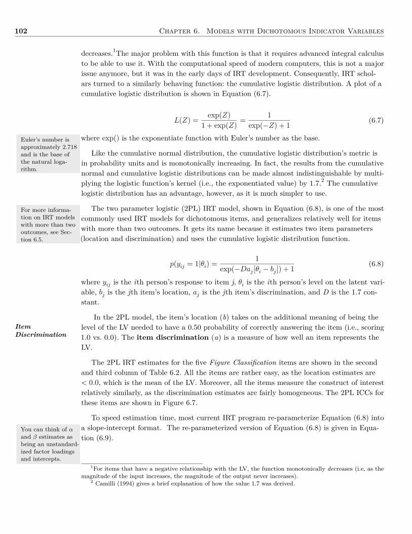
102 Chapter 6. Models with Dichotomous Indicator Variables
Euler’s number isapproximately 2.718and is the base ofthe natural loga-rithm.
For more informa-tion on IRT modelswith more than twooutcomes, see Sec-tion 6.5.
ItemDiscrimination
You can think of αand β estimates asbeing an unstandard-ized factor loadingsand intercepts.
decreases.1The major problem with this function is that it requires advanced integral calculusto be able to use it. With the computational speed of modern computers, this is not a majorissue anymore, but it was in the early days of IRT development. Consequently, IRT schol-ars turned to a similarly behaving function: the cumulative logistic distribution. A plot of acumulative logistic distribution is shown in Equation (6.7).
L(Z) = exp(Z)1 + exp(Z) = 1
exp(−Z) + 1 (6.7)
where exp() is the exponentiate function with Euler’s number as the base.
Like the cumulative normal distribution, the cumulative logistic distribution’s metric isin probability units and is monotonically increasing. In fact, the results from the cumulativenormal and cumulative logistic distributions can be made almost indistinguishable by multi-plying the logistic function’s kernel (i.e., the exponentiated value) by 1.7.2 The cumulativelogistic distribution has an advantage, however, as it is much simpler to use.
The two parameter logistic (2PL) IRT model, shown in Equation (6.8), is one of the mostcommonly used IRT models for dichotomous items, and generalizes relatively well for itemswith more than two outcomes. It gets its name because it estimates two item parameters(location and discrimination) and uses the cumulative logistic distribution function.
p(yij = 1|θi) = 1exp(−Daj [θi − bj ]) + 1 (6.8)
where yij is the ith person’s response to item j, θi is the ith person’s level on the latent vari-able, bj is the jth item’s location, aj is the jth item’s discrimination, and D is the 1.7 con-stant.
In the 2PL model, the item’s location (b) takes on the additional meaning of being thelevel of the LV needed to have a 0.50 probability of correctly answering the item (i.e., scoring1.0 vs. 0.0). The item discrimination (a) is a measure of how well an item represents theLV.
The 2PL IRT estimates for the five Figure Classification items are shown in the secondand third column of Table 6.2. All the items are rather easy, as the location estimates are< 0.0, which is the mean of the LV. Moreover, all the items measure the construct of interestrelatively similarly, as the discrimination estimates are fairly homogeneous. The 2PL ICCs forthese items are shown in Figure 6.7.
To speed estimation time, most current IRT program re-parameterize Equation (6.8) intoa slope-intercept format. The re-parameterized version of Equation (6.8) is given in Equa-tion (6.9).
1For items that have a negative relationship with the LV, the function monotonically decreases (i.e, as themagnitude of the input increases, the magnitude of the output never increases).
2 Camilli (1994) gives a brief explanation of how the value 1.7 was derived.
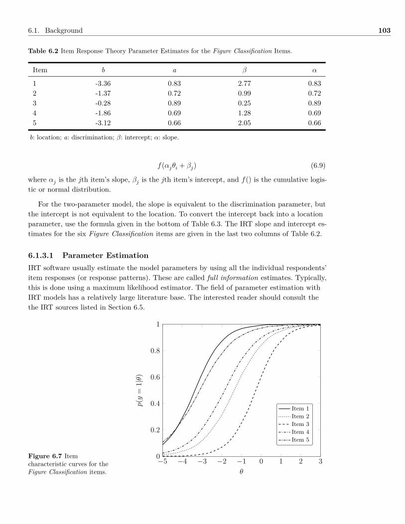
6.1. Background 103
Table 6.2 Item Response Theory Parameter Estimates for the Figure Classification Items.
Item b a β α
1 -3.36 0.83 2.77 0.832 -1.37 0.72 0.99 0.723 -0.28 0.89 0.25 0.894 -1.86 0.69 1.28 0.695 -3.12 0.66 2.05 0.66
b: location; a: discrimination; β: intercept; α: slope.
f(αjθi + βj) (6.9)
where αj is the jth item’s slope, βj is the jth item’s intercept, and f() is the cumulative logis-tic or normal distribution.
For the two-parameter model, the slope is equivalent to the discrimination parameter, butthe intercept is not equivalent to the location. To convert the intercept back into a locationparameter, use the formula given in the bottom of Table 6.3. The IRT slope and intercept es-timates for the six Figure Classification items are given in the last two columns of Table 6.2.
6.1.3.1 Parameter EstimationIRT software usually estimate the model parameters by using all the individual respondents’item responses (or response patterns). These are called full information estimates. Typically,this is done using a maximum likelihood estimator. The field of parameter estimation withIRT models has a relatively large literature base. The interested reader should consult thethe IRT sources listed in Section 6.5.
Figure 6.7 Itemcharacteristic curves for theFigure Classification items.
−5 −4 −3 −2 −1 0 1 2 30
0.2
0.4
0.6
0.8
1
θ
p(y
=1|θ)
Item 1Item 2Item 3Item 4Item 5
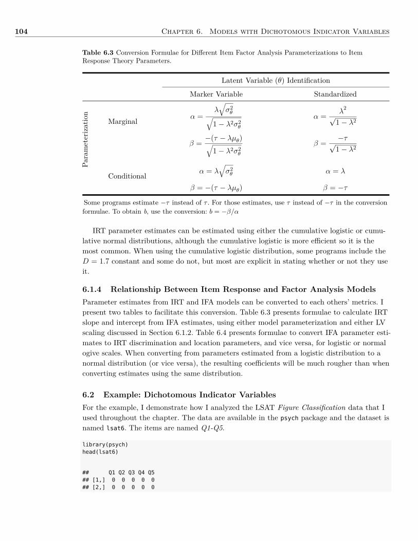
104 Chapter 6. Models with Dichotomous Indicator Variables
Table 6.3 Conversion Formulae for Different Item Factor Analysis Parameterizations to ItemResponse Theory Parameters.
Latent Variable (θ) Identification
Marker Variable StandardizedPa
rameterization
Marginal α =λ√σ2θ√
1− λ2σ2θ
α = λ2
√1− λ2
β = −(τ − λµθ)√1− λ2σ2
θ
β = −τ√1− λ2
Conditional α = λ√σ2θ α = λ
β = −(τ − λµθ) β = −τ
Some programs estimate −τ instead of τ . For those estimates, use τ instead of −τ in the conversionformulae. To obtain b, use the conversion: b = −β/α
IRT parameter estimates can be estimated using either the cumulative logistic or cumu-lative normal distributions, although the cumulative logistic is more efficient so it is themost common. When using the cumulative logistic distribution, some programs include theD = 1.7 constant and some do not, but most are explicit in stating whether or not they useit.
6.1.4 Relationship Between Item Response and Factor Analysis ModelsParameter estimates from IRT and IFA models can be converted to each others’ metrics. Ipresent two tables to facilitate this conversion. Table 6.3 presents formulae to calculate IRTslope and intercept from IFA estimates, using either model parameterization and either LVscaling discussed in Section 6.1.2. Table 6.4 presents formulae to convert IFA parameter esti-mates to IRT discrimination and location parameters, and vice versa, for logistic or normalogive scales. When converting from parameters estimated from a logistic distribution to anormal distribution (or vice versa), the resulting coefficients will be much rougher than whenconverting estimates using the same distribution.
6.2 Example: Dichotomous Indicator VariablesFor the example, I demonstrate how I analyzed the LSAT Figure Classification data that Iused throughout the chapter. The data are available in the psych package and the dataset isnamed lsat6. The items are named Q1-Q5.
library(psych)head(lsat6)
## Q1 Q2 Q3 Q4 Q5## [1,] 0 0 0 0 0## [2,] 0 0 0 0 0
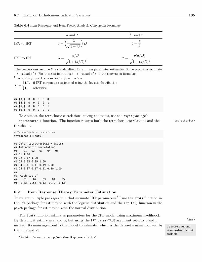
6.2. Example: Dichotomous Indicator Variables 105
Table 6.4 Item Response and Item Factor Analysis Conversion Formulae.
a and λ b1 and τ
IFA to IRT a =(
λ√1− λ2
)D b = τ
λ
IRT to IFA λ = a/D√1 + (a/D)2
τ = b(a/D)√1 + (a/D)2
The conversions assume θ is standardized for all item parameter estimates. Some programs estimate−τ instead of τ . For those estimates, use −τ instead of τ in the conversion formulae.1 To obtain β, use the conversion: β = −α × b.
D ={
1.7, if IRT parameters estimated using the logistic distribution1, otherwise
## [3,] 0 0 0 0 0## [4,] 0 0 0 0 1## [5,] 0 0 0 0 1## [6,] 0 0 0 0 1
To estimate the tetrachoric correlations among the items, use the psych package’stetrachoric() function. The function returns both the tetrachoric correlations and the
thresholds.
# Tetrachoric correlationstetrachoric(lsat6)
## Call: tetrachoric(x = lsat6)## tetrachoric correlation## Q1 Q2 Q3 Q4 Q5## Q1 1.00## Q2 0.17 1.00## Q3 0.23 0.19 1.00## Q4 0.11 0.11 0.19 1.00## Q5 0.07 0.17 0.11 0.20 1.00#### with tau of## Q1 Q2 Q3 Q4 Q5## -1.43 -0.55 -0.13 -0.72 -1.13
6.2.1 Item Response Theory Parameter EstimationThere are multiple packages in R that estimate IRT parameters.3 I use the ltm() function inthe ltm package for estimation with the logistic distribution and the irt.fa() function in thepsych package for estimation with the normal distribution.
The ltm() function estimates parameters for the 2PL model using maximum likelihood.By default, it estimates β and α, but using the IRT.param=TRUE argument returns b and ainstead. Its main argument is the model to estimate, which is the dataset’s name followed bythe tilde and z1.
tetrachoric()
ltm()
z1 represents onestandardized latentvariable.
3See http://cran.cc.uoc.gr/web/views/Psychometrics.html
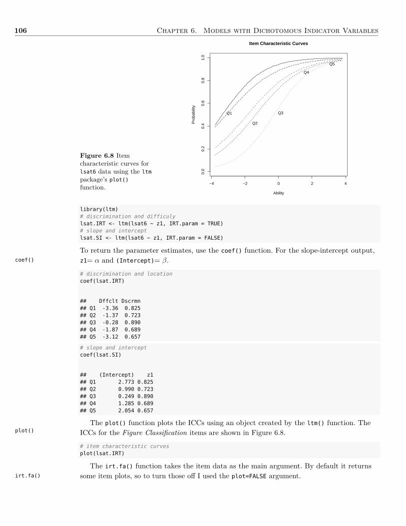
106 Chapter 6. Models with Dichotomous Indicator Variables
Figure 6.8 Itemcharacteristic curves forlsat6 data using the ltm
package’s plot()
function.−4 −2 0 2 4
0.0
0.2
0.4
0.6
0.8
1.0
Item Characteristic Curves
AbilityP
roba
bilit
y
Q1
Q2
Q3
Q4
Q5
coef()
plot()
irt.fa()
library(ltm)# discrimination and difficulylsat.IRT <- ltm(lsat6 ~ z1, IRT.param = TRUE)# slope and interceptlsat.SI <- ltm(lsat6 ~ z1, IRT.param = FALSE)
To return the parameter estimates, use the coef() function. For the slope-intercept output,z1= α and (Intercept)= β.
# discrimination and locationcoef(lsat.IRT)
## Dffclt Dscrmn## Q1 -3.36 0.825## Q2 -1.37 0.723## Q3 -0.28 0.890## Q4 -1.87 0.689## Q5 -3.12 0.657
# slope and interceptcoef(lsat.SI)
## (Intercept) z1## Q1 2.773 0.825## Q2 0.990 0.723## Q3 0.249 0.890## Q4 1.285 0.689## Q5 2.054 0.657
The plot() function plots the ICCs using an object created by the ltm() function. TheICCs for the Figure Classification items are shown in Figure 6.8.
# item characteristic curvesplot(lsat.IRT)
The irt.fa() function takes the item data as the main argument. By default it returnssome item plots, so to turn those off I used the plot=FALSE argument.
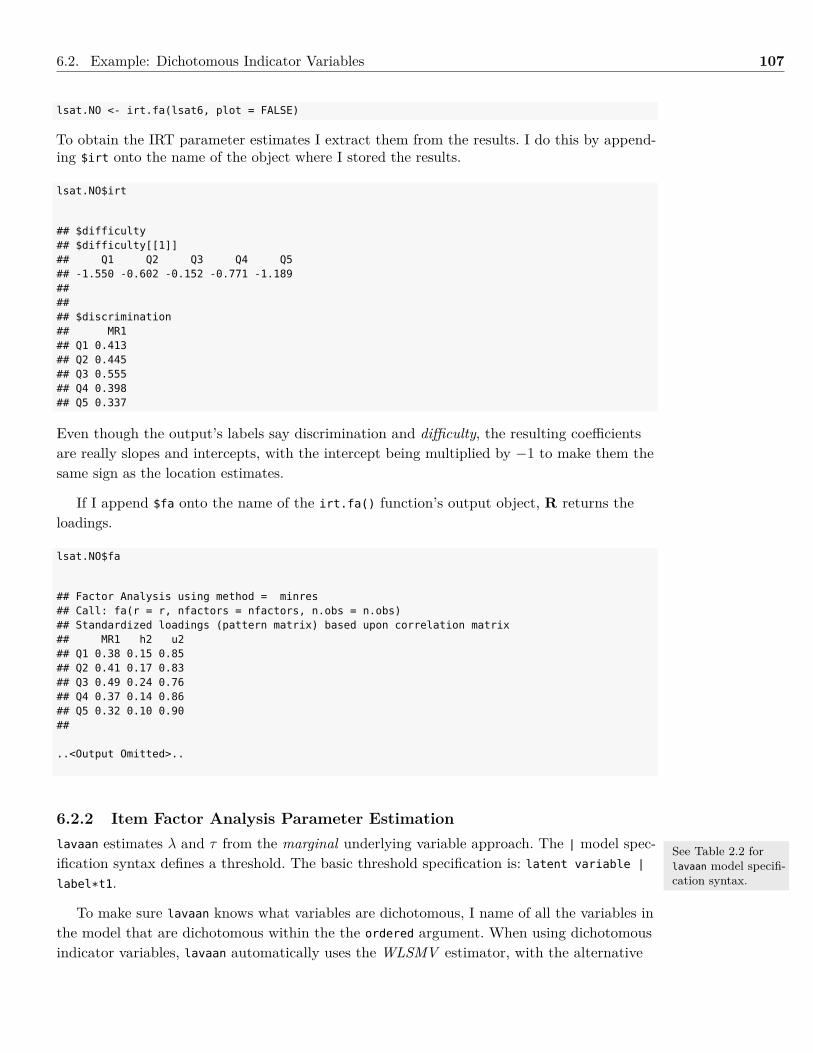
6.2. Example: Dichotomous Indicator Variables 107
lsat.NO <- irt.fa(lsat6, plot = FALSE)
To obtain the IRT parameter estimates I extract them from the results. I do this by append-ing $irt onto the name of the object where I stored the results.
lsat.NO$irt
## $difficulty## $difficulty[[1]]## Q1 Q2 Q3 Q4 Q5## -1.550 -0.602 -0.152 -0.771 -1.189###### $discrimination## MR1## Q1 0.413## Q2 0.445## Q3 0.555## Q4 0.398## Q5 0.337
Even though the output’s labels say discrimination and difficulty, the resulting coefficientsare really slopes and intercepts, with the intercept being multiplied by −1 to make them thesame sign as the location estimates.
If I append $fa onto the name of the irt.fa() function’s output object, R returns theloadings.
lsat.NO$fa
## Factor Analysis using method = minres## Call: fa(r = r, nfactors = nfactors, n.obs = n.obs)## Standardized loadings (pattern matrix) based upon correlation matrix## MR1 h2 u2## Q1 0.38 0.15 0.85## Q2 0.41 0.17 0.83## Q3 0.49 0.24 0.76## Q4 0.37 0.14 0.86## Q5 0.32 0.10 0.90##
..<Output Omitted>..
6.2.2 Item Factor Analysis Parameter Estimationlavaan estimates λ and τ from the marginal underlying variable approach. The | model spec-ification syntax defines a threshold. The basic threshold specification is: latent variable |
label*t1.
To make sure lavaan knows what variables are dichotomous, I name of all the variables inthe model that are dichotomous within the the ordered argument. When using dichotomousindicator variables, lavaan automatically uses the WLSMV estimator, with the alternative
See Table 2.2 forlavaan model specifi-cation syntax.
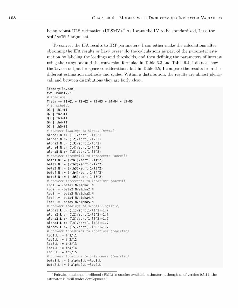
108 Chapter 6. Models with Dichotomous Indicator Variables
being robust ULS estimation (ULSMV).4 As I want the LV to be standardized, I use thestd.lv=TRUE argument.
To convert the IFA results to IRT parameters, I can either make the calculations afterobtaining the IFA results or have lavaan do the calculations as part of the parameter esti-mation by labeling the loadings and thresholds, and then defining the parameters of interestusing the := syntax and the conversion formulae in Table 6.3 and Table 6.4. I do not showthe lavaan output for space considerations, but in Table 6.5, I compare the results from thedifferent estimation methods and scales. Within a distribution, the results are almost identi-cal, and between distributions they are fairly close.
library(lavaan)twoP.model<-'# loadingsTheta =~ l1*Q1 + l2*Q2 + l3*Q3 + l4*Q4 + l5*Q5# thresholdsQ1 | th1*t1Q2 | th2*t1Q3 | th3*t1Q4 | th4*t1Q5 | th5*t1# convert loadings to slopes (normal)alpha1.N := (l1)/sqrt(1-l1^2)alpha2.N := (l2)/sqrt(1-l2^2)alpha3.N := (l3)/sqrt(1-l3^2)alpha4.N := (l4)/sqrt(1-l4^2)alpha5.N := (l5)/sqrt(1-l5^2)# convert thresholds to intercepts (normal)beta1.N := (-th1)/sqrt(1-l1^2)beta2.N := (-th2)/sqrt(1-l2^2)beta3.N := (-th3)/sqrt(1-l3^2)beta4.N := (-th4)/sqrt(1-l4^2)beta5.N := (-th5)/sqrt(1-l5^2)# convert intercepts to locations (normal)loc1 := -beta1.N/alpha1.Nloc2 := -beta2.N/alpha2.Nloc3 := -beta3.N/alpha3.Nloc4 := -beta4.N/alpha4.Nloc5 := -beta5.N/alpha5.N# convert loadings to slopes (logistic)alpha1.L := (l1)/sqrt(1-l1^2)*1.7alpha2.L := (l2)/sqrt(1-l2^2)*1.7alpha3.L := (l3)/sqrt(1-l3^2)*1.7alpha4.L := (l4)/sqrt(1-l4^2)*1.7alpha5.L := (l5)/sqrt(1-l5^2)*1.7# convert thresholds to locations (logistic)loc1.L := th1/l1loc2.L := th2/l2loc3.L := th3/l3loc4.L := th4/l4loc5.L := th5/l5# convert locations to intercepts (logistic)beta1.L := (-alpha1.L)*loc1.Lbeta2.L := (-alpha2.L)*loc2.L
4Pairwise maximum likelihood (PML) is another available estimator, although as of version 0.5.14, theestimator is “still under development.”
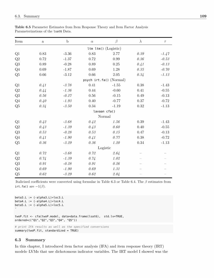
6.3. Summary 109
Table 6.5 Parameter Estimates from Item Response Theory and Item Factor AnalysisParameterizations of the lsat6 Data.
Item a b α β λ τ
ltm ltm() (Logistic)Q1 0.83 -3.36 0.83 2.77 0.39 -1.47Q2 0.72 -1.37 0.72 0.99 0.36 -0.53Q3 0.89 -0.28 0.89 0.25 0.41 -0.13Q4 0.69 -1.87 0.69 1.28 0.35 -0.70Q5 0.66 -3.12 0.66 2.05 0.34 -1.13
psych irt.fa() (Normal)Q1 0.41 -3.78 0.41 -1.55 0.38 -1.43Q2 0.44 -1.36 0.44 -0.60 0.41 -0.55Q3 0.56 -0.27 0.56 -0.15 0.49 -0.13Q4 0.40 -1.93 0.40 -0.77 0.37 -0.72Q5 0.34 -3.50 0.34 -1.19 0.32 -1.13
lavaan cfa()
NormalQ1 0.42 -3.68 0.42 1.56 0.39 -1.43Q2 0.43 -1.39 0.43 0.60 0.40 -0.55Q3 0.53 -0.28 0.53 0.15 0.47 -0.13Q4 0.41 -1.90 0.41 0.77 0.38 -0.72Q5 0.36 -3.29 0.36 1.20 0.34 -1.13
LogisticQ1 0.72 -3.68 0.72 2.64 – –Q2 0.74 -1.39 0.74 1.02 – –Q3 0.91 -0.28 0.91 0.26 – –Q4 0.69 -1.90 0.69 1.31 – –Q5 0.62 -3.29 0.62 2.04 – –
Italicized coefficients were converted using formulae in Table 6.3 or Table 6.4. The β estimates fromirt.fa() are −1(β).
beta3.L := (-alpha3.L)*loc3.Lbeta4.L := (-alpha4.L)*loc4.Lbeta5.L := (-alpha5.L)*loc5.L'
twoP.fit <- cfa(twoP.model, data=data.frame(lsat6), std.lv=TRUE,ordered=c("Q1","Q2","Q3","Q4", "Q5"))
# print IFA results as well as the specified conversionssummary(twoP.fit, standardized = TRUE)
6.3 SummaryIn this chapter, I introduced item factor analysis (IFA) and item response theory (IRT)models–LVMs that use dichotomous indicator variables. The IRT model I showed was the
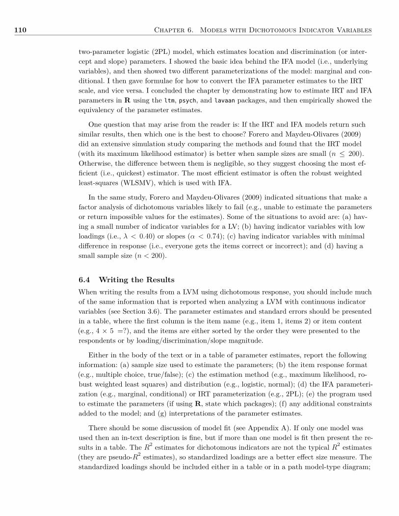
110 Chapter 6. Models with Dichotomous Indicator Variables
two-parameter logistic (2PL) model, which estimates location and discrimination (or inter-cept and slope) parameters. I showed the basic idea behind the IFA model (i.e., underlyingvariables), and then showed two different parameterizations of the model: marginal and con-ditional. I then gave formulae for how to convert the IFA parameter estimates to the IRTscale, and vice versa. I concluded the chapter by demonstrating how to estimate IRT and IFAparameters in R using the ltm, psych, and lavaan packages, and then empirically showed theequivalency of the parameter estimates.
One question that may arise from the reader is: If the IRT and IFA models return suchsimilar results, then which one is the best to choose? Forero and Maydeu-Olivares (2009)did an extensive simulation study comparing the methods and found that the IRT model(with its maximum likelihood estimator) is better when sample sizes are small (n ≤ 200).Otherwise, the difference between them is negligible, so they suggest choosing the most ef-ficient (i.e., quickest) estimator. The most efficient estimator is often the robust weightedleast-squares (WLSMV), which is used with IFA.
In the same study, Forero and Maydeu-Olivares (2009) indicated situations that make afactor analysis of dichotomous variables likely to fail (e.g., unable to estimate the parametersor return impossible values for the estimates). Some of the situations to avoid are: (a) hav-ing a small number of indicator variables for a LV; (b) having indicator variables with lowloadings (i.e., λ < 0.40) or slopes (α < 0.74); (c) having indicator variables with minimaldifference in response (i.e., everyone gets the items correct or incorrect); and (d) having asmall sample size (n < 200).
6.4 Writing the ResultsWhen writing the results from a LVM using dichotomous response, you should include muchof the same information that is reported when analyzing a LVM with continuous indicatorvariables (see Section 3.6). The parameter estimates and standard errors should be presentedin a table, where the first column is the item name (e.g., item 1, items 2) or item content(e.g., 4 × 5 =?), and the items are either sorted by the order they were presented to therespondents or by loading/discrimination/slope magnitude.
Either in the body of the text or in a table of parameter estimates, report the followinginformation: (a) sample size used to estimate the parameters; (b) the item response format(e.g., multiple choice, true/false); (c) the estimation method (e.g., maximum likelihood, ro-bust weighted least squares) and distribution (e.g., logistic, normal); (d) the IFA parameteri-zation (e.g., marginal, conditional) or IRT parameterization (e.g., 2PL); (e) the program usedto estimate the parameters (if using R, state which packages); (f) any additional constraintsadded to the model; and (g) interpretations of the parameter estimates.
There should be some discussion of model fit (see Appendix A). If only one model wasused then an in-text description is fine, but if more than one model is fit then present the re-sults in a table. The R2 estimates for dichotomous indicators are not the typical R2 estimates(they are pseudo-R2 estimates), so standardized loadings are a better effect size measure. Thestandardized loadings should be included either in a table or in a path model-type diagram;
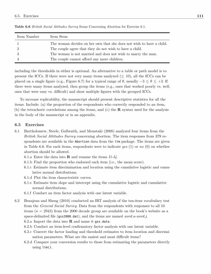
6.5. Exercises 111
Table 6.6 British Social Attitudes Survey Items Concerning Abortion for Exercise 6.1.
Item Number Item Stem
1 The woman decides on her own that she does not wish to have a child.2 The couple agree that they do not wish to have a child.3 The woman is not married and does not wish to marry the man.4 The couple cannot afford any more children.
including the thresholds in either is optional. An alternative to a table or path model is topresent the ICCs. If there were not very many items analyzed (≤ 10), all the ICCs can beplaced on a single figure (e.g., Figure 6.7) for a typical range of θ, usually −3 ≤ θ ≤ +3. Ifthere were many items analyzed, then group the items (e.g., ones that worked poorly vs. well,ones that were easy vs. difficult) and show multiple figures with the grouped ICCs.
To increase replicability, the manuscript should present descriptive statistics for all theitems. Include: (a) the proportion of the respondents who correctly responded to an item,(b) the tetrachoric correlations among the items, and (c) the R syntax used for the analysisin the body of the manuscript or in an appendix.
6.5 Exercises6.1 Bartholomew, Steele, Galbraith, and Moustaki (2008) analyzed four items from the
British Social Attitudes Survey concerning abortion. The item responses from 379 re-spondents are available in the Abortion data from the ltm package. The items are givenin Table 6.6. For each items, respondents were to indicate yes (1) or no (0) on whetherabortion should be allowed.6.1.a Enter the data into R and rename the items I1-I4.6.1.b Find the proportion who endorsed each item (i.e., the mean score).6.1.c Estimate item discrimination and location using the cumulative logistic and cumu-
lative normal distributions.6.1.d Plot the item characteristic curves.6.1.e Estimate item slope and intercept using the cumulative logistic and cumulative
normal distributions.6.1.f Conduct an item factor analysis with one latent variable.
6.2 Beaujean and Sheng (2010) conducted an IRT analysis of the ten-item vocabulary testfrom the General Social Survey. Data from the respondents with responses to all 10items (n = 2943) from the 2000 decade group are available on the book’s website as aspace-delimited file (gss2000.dat), and the items are named word.a-word.j.6.2.a Import the data into R and name it gss.data.6.2.b Conduct an item-level confirmatory factor analysis with one latent variable.6.2.c Convert the factor loading and threshold estimates to item location and discrimi-
nation parameters. What are the easiest and most difficult items?6.2.d Compare your conversion results to those from estimating the parameters directly
using ltm().
112 Chapter 6. Models with Dichotomous Indicator Variables
6.6 References & Further ReadingsBaker, F. B., & Kim, S.-H. (2004). Item response theory: Parameter estimation techniques
(2nd ed.). New York, NY: Mercel Dekker.Bartholomew, D. J., Knott, M., & Moustaki, I. (2011). Latent variable models and factor
analysis: A unified approach (3rd ed.). New York, NY: John Wiley & Sons.Bartholomew, D. J., Steele, F., Galbraith, J., & Moustaki, I. (2008). Analysis of multivariate
social science data (2nd ed.). Boca Raton, FL: Chapman and Hall/CRC.Beauducel, A., & Herzberg, P. Y. (2006). On the performance of maximum likelihood versus
means and variance adjusted weighted least squares estimation in CFA. StructuralEquation Modeling: A Multidisciplinary Journal, 13 , 186-203. doi:10.1207/s15328007sem1302_2
Beaujean, A. A., & Sheng, Y. (2010). Examining the Flynn effect in the general social surveyvocabulary test using item response theory. Personality and Individual Differences, 48 ,294-298. doi: 10.1016/j.paid.2009.10.019
Bock, R. D., & Lieberman, M. (1970). Fitting a response model for n dichotomously scoreditems. Psychometrika, 35 , 179-197. doi: 10.1007/BF02291262
Camilli, G. (1994). Teacher’s corner: Origin of the scaling constant d = 1.7 in item responsetheory. Journal of Educational and Behavioral Statistics, 19 , 293-295. doi:10.3102/10769986019003293
Embretson, S. E., & Reise, S. P. (2000). Item response theory for psychologists. Mahwah, NJ:Erlbaum.
Finney, S. J., & DiStefano, C. (2013). Non-normal and categorical data in structural equationmodeling. In G. R. Hancock & R. O. Mueller (Eds.), Structural equation modeling: Asecond course (2nd ed.). Charolette, NC: Information Age Publishing.
Flora, D. B., & Curran, P. J. (2004). An empirical evaluation of alternative methods ofestimation for confirmatory factor analysis with ordinal data. Psychological Methods, 9 ,466-491. doi: 10.1037/1082-989X.9.4.466
Forero, C. G., & Maydeu-Olivares, A. (2009). Estimation of IRT graded response models:Limited versus full information methods. Psychological Methods, 14 , 275-299. doi:10.1037/a0015825
Guttman, L. (1950). The basis for scalogram analysis. In S. A. Stouffer, L. Guttman,E. A. Suchman, P. F. Lazarsfeld, S. A. Star, & J. A. Clausen (Eds.), Measurement andprediction (pp. 60–90). Princeton, NJ: Princeton University Press.
Kamata, A., & Bauer, D. J. (2008). A note on the relation between factor analytic and itemresponse theory models. Structural Equation Modeling: A Multidisciplinary Journal, 15 ,136-153. doi: 10.1080/10705510701758406
Reese, L. M., & Cotter, R. A. (1994). A compendium of LSAT and LSAC-sponsored item types(Tech. Rep. No. LSAC-RR-94-01). Newton, PA: Law School Admission Council.
Rhemtulla, M., Brosseau-Liard, P. E., & Savalei, V. (2012). When can categorical variables betreated as continuous? A comparison of robust continuous and categorical SEMestimation methods under suboptimal conditions. Psychological Methods, 17 , 354-373.doi: 10.1037/a0029315

6.6. References & Further Readings 113
Rizopoulos, D. (2006). ltm: An R package for latent variable modeling and item responsetheory analyses. Journal of Statistical Software, 17 (5), 1-25. Retrieved fromhttp://www.jstatsoft.org/v17/i05/.
West, S. G., Finch, J. F., & Curran, P. J. (1995). Structural equation models with non-normalvariables: Problems and remedies. In R. A. Hoyle (Ed.), Structural equation modeling:Concepts, issues and applications (pp. 56–75). Newbury Park, CA: Sage.
Wirth, R. J., & Edwards, M. C. (2007). Item factor analysis: Current approaches and futuredirections. Psychological Methods, 12 , 58-79. doi: 10.1037/1082-989x.12.1.58
Missing DataPattern
7 | Models with Missing Data
Chapter Contents7.1 Background . . . . . . . . . . . . . . . . . . . . . . . . . . . . . . . . . . . . 114
7.1.1 Types of Missing Data . . . . . . . . . . . . . . . . . . . . . . . . . . 1147.2 Analyzing Data With Missing Values . . . . . . . . . . . . . . . . . . . . . . 117
7.2.1 Traditional Methods . . . . . . . . . . . . . . . . . . . . . . . . . . . 1187.2.2 Modern Methods . . . . . . . . . . . . . . . . . . . . . . . . . . . . . 1197.2.3 Auxiliary Variables . . . . . . . . . . . . . . . . . . . . . . . . . . . . 121
7.3 Example: Missing Data . . . . . . . . . . . . . . . . . . . . . . . . . . . . . . 1217.4 Summary . . . . . . . . . . . . . . . . . . . . . . . . . . . . . . . . . . . . . . 1287.5 Writing the Results . . . . . . . . . . . . . . . . . . . . . . . . . . . . . . . . 1287.6 Exercises . . . . . . . . . . . . . . . . . . . . . . . . . . . . . . . . . . . . . . 1287.7 References & Further Readings . . . . . . . . . . . . . . . . . . . . . . . . . . 130
7.1 BackgroundMissing data are almost inevitable in any research project, especially those involving humans.Depending on the pattern and amount of missing data, excluding these incomplete observa-tions can seriously bias parameter estimates or diminish sample size. Consequently, missingdata needs to be assessed and, if found, addressed in every study.
It will make the presentation of missing data types and methods for handling them easierif I first present a motivational example. In this example, I am interested in understandingthe influence of an academic intervention on reading ability in elementary school students.I randomly assigned half of the students to receive the intervention and the other half toreceive typical reading instruction. I conceptualized reading ability as a latent variable, andgathered data on three indicator variables: word reading, pseudoword reading, and readingcomprehension. A path model of this example is shown in Figure 7.1.
7.1.1 Types of Missing DataLittle and Rubin (2002) posited three types of missing data: (a) missing completely at ran-dom (MCAR) (b) missing at random (MAR); and (c) not missing at random (NMAR). Thesethree types of missing data are not mutually exclusive categories, though. In fact, Graham(2009) argued that pure versions of the typologies never really exist, so it is better to thinkof missing data as being on a continuum between them. Thus, the question is not what typeof missing data is present in a dataset, but if the pattern of missingness precludes being ableto use modern techniques to handle the missing data (see Section 7.2). A missing data pat-tern is the configuration of observed and missing values in a dataset.
7.1.1.1 Missing Completely at RandomData are missing completely at random (MCAR) when the missing values on a givenvariable (i.e, its missingness) are unrelated to both that variable and any other variable in
114
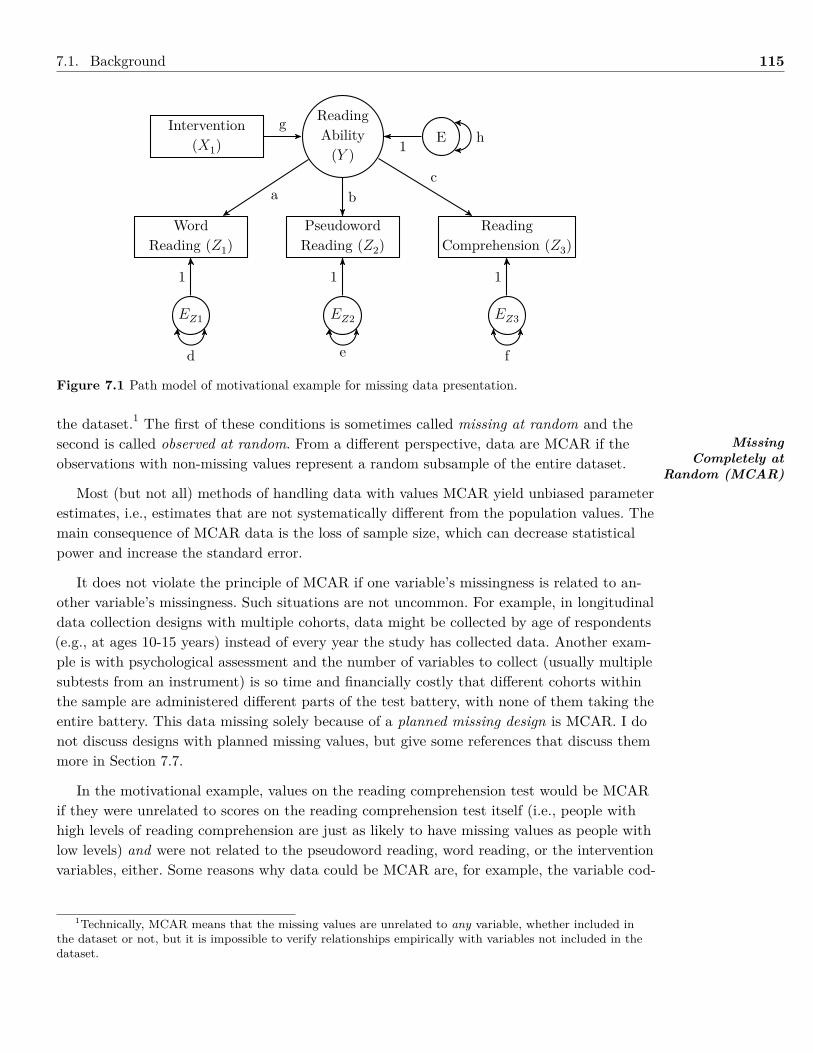
7.1. Background 115
ReadingAbility(Y )
PseudowordReading (Z2)
WordReading (Z1)
ReadingComprehension (Z3)
EIntervention
(X1)
a bc
1g
EZ1 EZ2 EZ3
1 1 1
d e f
h
Figure 7.1 Path model of motivational example for missing data presentation.
the dataset.1 The first of these conditions is sometimes called missing at random and thesecond is called observed at random. From a different perspective, data are MCAR if theobservations with non-missing values represent a random subsample of the entire dataset.
Most (but not all) methods of handling data with values MCAR yield unbiased parameterestimates, i.e., estimates that are not systematically different from the population values. Themain consequence of MCAR data is the loss of sample size, which can decrease statisticalpower and increase the standard error.
It does not violate the principle of MCAR if one variable’s missingness is related to an-other variable’s missingness. Such situations are not uncommon. For example, in longitudinaldata collection designs with multiple cohorts, data might be collected by age of respondents(e.g., at ages 10-15 years) instead of every year the study has collected data. Another exam-ple is with psychological assessment and the number of variables to collect (usually multiplesubtests from an instrument) is so time and financially costly that different cohorts withinthe sample are administered different parts of the test battery, with none of them taking theentire battery. This data missing solely because of a planned missing design is MCAR. I donot discuss designs with planned missing values, but give some references that discuss themmore in Section 7.7.
In the motivational example, values on the reading comprehension test would be MCARif they were unrelated to scores on the reading comprehension test itself (i.e., people withhigh levels of reading comprehension are just as likely to have missing values as people withlow levels) and were not related to the pseudoword reading, word reading, or the interventionvariables, either. Some reasons why data could be MCAR are, for example, the variable cod-
MissingCompletely at
Random (MCAR)
1Technically, MCAR means that the missing values are unrelated to any variable, whether included inthe dataset or not, but it is impossible to verify relationships empirically with variables not included in thedataset.
116 Chapter 7. Models with Missing Data
Section 7.7 has somereferences on inter-preting odds ratiosand using R for alogistic regression.
Missing atRandom (MAR)
I briefly mentionedMAR data in Sec-tion 7.1.1.1 as partof the MCAR defini-tion. Thus, MCARis really just a spe-cific type of MAR.
ing process had random input errors or a respondent got ill just before the test and did notcomplete the test later. The key is that there is no systematic reason why data are missing.
I can empirically evaluate if data are MCAR, and it is the only missing data mechanismthat is testable. There are two approaches to doing this: univariate and multivariate. Theunivariate approach requires creating dummy codes for each variable that has missing values(e.g., 0 = missing, 1 = present), then doing one of two procedures. First, using each dummy-coded variable to represent group membership, calculate the effect size for the between-groups mean differences (e.g., the d or g effect sizes) for each dummy-coded variable, sepa-rately. If the effect size is small (< 0.15− 0.20), this suggests that there is no systematic differ-ence between responders and non-responders on other variables in the dataset, which wouldgive some support for the data being MCAR. The second procedure involves doing a logisticregression, regressing each dummy-coded variable (separately) onto the other variables in thedataset. Having no large odds ratios (an effect size for logistic regression) indicates the dataon the dummy-coded outcome are MCAR.
As an alternative to doing many univariate comparisons, Little (1988) proposed a multi-variate test statistic for MCAR that is akin to simultaneously testing all the mean differences.Although it has not been tested extensively, what has been done has tended to support thatthe Type 1 error rate (i.e., saying the data is MCAR when is it not) is relatively stable acrosssample sizes, number of variables, and amount of missing data. The problem with both theunivariate and multivariate methods, though, is that they only test for mean differences, notdifferences in (co)variances. Thus, they do not asses whether the relationships among thevariables is the same for responders and non-responders. Fortunately, there has been somerecent developments in this area, both theoretically and in R, which I discuss more in Sec-tion 7.3.
7.1.1.2 Missing At RandomAssuming values are MCAR is often unreasonable for many studies because missing val-ues are usually related to other variables if enough pertinent information is collected (e.g.,sex, education status, age). Thus, a second type of missing data is missing at random(MAR). Data are MAR if a given variable’s missingness is unrelated to the variable itself, butis related to other variables in the dataset. Thus, MAR assumes that the variables that ex-plain the missing data are included in the analysis either as predictors, outcomes, or auxiliaryvariables (more on auxiliary variables in Section 7.2.3). If handled appropriately, analysis ofMAR data can yield unbiased parameter estimates.
In the motivational example, data on the reading comprehension variable would be MARif students with high, average, or low reading comprehension scores were equally as likely tohave missing responses, but students with low word reading scores had missing reading com-prehension scores more often than students with average or high word reading scores. Withina word reading performance group, however, there is no relationship between missingnessand reading comprehension scores. Thus, for analyses of MAR data to work properly, thevariables related to the missingness need to be included in the analysis model.
7.2. Analyzing Data With Missing Values 117
Unlike MCAR, there is no test for values being MAR. Nonetheless, it can be useful to ex-amine if any of the variables in the dataset are related to the missing responses. The logisticregression method discussed in Section 7.1.1.1 is a decent method for doing this.
7.1.1.3 Not Missing at RandomData are not missing at random (NMAR) (sometimes called non-ignorable or missing notat random) if the missing values are not MCAR or MAR. More concretely, data are NMAR ifa variable’s missingness is related to that variable, even after including all possible covariatesin the model. Values that are NMAR are a problem because they yield biased parameterestimates with traditional techniques and could yield biased results with modern techniquesas well. Thus, the modern techniques I discuss in this chapter could work or it could requiremore complex techniques (e.g., instrumental variables, mixture modeling). The references inSection 7.7 describe some alternative techniques for data NMAR.
In the motivational example, if students with lower reading comprehension skills weremore likely to have missing reading comprehension scores than students with higher skills,then the data on this variable would be NMAR. The problem, though, is that I do not knowwhat the students’ reading comprehension skills really are because I do not have their scores!Thus, NMAR is more of a conceptual consideration than a empirical one: Are students withlow reading comprehension scores more likely to have missing data (e.g., absent when the testwas administered, leave the study before taking this test)? This does not mean there are nodata to examine, though. For example, I might observe that participants who have low scoreson the reading portion of the state achievement test also have high rates of missing values onthe reading comprehension test, which would provide some evidence that the data are likelyNMAR.
7.2 Analyzing Data With Missing ValuesIf there are missing responses in a dataset, the best method to deal with them is a func-tion of: (a) the type of missing data (see Section 7.1.1); (b) how much data are missing; and(c) the variables that have missing values.
For example, if the data are MCAR and only make up a small percentage (i.e., < 3− 5%)of the entire dataset, and the sample size is relatively large (n > 200), then listwise deletion(see Section 7.2.1) will likely not have a noticeable influence on the parameter estimates. Asanother example, say the variable of interest is the average value of a group of items on aquestionnaire. The dataset contains all the item responses and a small percent of the itemresponses are missing. In such situations, it may be just as fine averaging the items that dohave responses rather than using one of the modern methods listed below.
Another consideration is the roles the variables with missing values have in the model.Missing data on an endogenous variable pose different problems from missing data on anexogenous variable. When the data are MAR, then observations with missing values on theendogenous variable, but have values for all the exogenous variables, do not contribute anyinformation to the outcome-predictor relationship. The information they provide is still use-ful, but they do not make a contribution to the path coefficient.
Not Missing AtRandom (NMAR)
A sensitivity anal-ysis could indicatewhether the modernmethods are appro-priate.
118 Chapter 7. Models with Missing Data
When initially ex-amining a dataset,listwise deletion isfine to use. A morerobust method typi-cally should be usedwhen conductingthe final (reported)analysis.
Consequently, there is not a one-size-fits-all method when dealing with missing values.Instead, it requires knowing how much data are missing on each variable, how the variablesare to be used in the analysis, and a reasoned belief for the types of missing values.
7.2.1 Traditional MethodsHistorically, missing data were addressed indirectly by one of two methods. First, observa-tions with missing data were deleted either listwise or pairwise. With listwise deletion (some-times called complete case analysis), observations (cases) with any missing values on vari-ables used in a model are deleted before estimating any parameters. This is the default pro-cedure for most statistical programs, including R. It provides unbiased parameter estimatesonly if data are MCAR. However, the price for removing entire observations is that the esti-mates’ standard errors increase (i.e., are less precise) and statistical power decreases.
With pairwise deletion (sometimes called available case analysis), the maximum amountof bivariate (pairwise) data available is retained for a single parameter estimate. This methodis usually employed to estimate means and covariances, which are then used for other analy-ses (e.g., regression, latent variable model). In such instances, an observation (case) that hasa missing value on one variable (A) would not be used to calculate the covariance betweenthat variable and another variable (A and B), but would be included in all other covarianceestimates (e.g., B and C ).
There are some major problems with pairwise deletion. First, since (potentially) differentobservations are used to calculate each covariance, this can lead to a situation where twoseparate (non-overlapping) subsets of a dataset’s observation are used for two covariance es-timates. Moreover, the covariance matrices estimated using pairwise deletion are more likelyto not return results or return impossible values (i.e., the matrix is singular/non-positive defi-nite) than other techniques for handling missing data. Finally, while the parameter estimatesfrom pairwise deletion may be unbiased if data are MCAR, it still leaves a big question unan-swered: What is the study’s sample size?
An American Psychological Association task force had this to say about listwise and pair-wise methods for handling missing data:
Special issues arise in modeling when we have missing data. The two popularmethods for dealing with missing data that are found in basic statistics packages,listwise and pairwise deletion of missing values, are among the worst methodsavailable for practical applications. (Wilkinson & American Psychological As-sociation Science Directorate Task Force on Statistical Inference, 1999, p. 598,emphasis added)
The second historical approach to handling missing data was imputation, which replaces amissing value with another plausible value, typically based on one of three strategies: (a) themean/median of all present values of the variable; (b) regression-based predicted scores (us-ing all the other variables in the dataset as predictors); or (c) use a pattern-matching tech-nique to find another observation that has similar responses across all the other variables in
7.2. Analyzing Data With Missing Values 119
the dataset, and then replace the missing value with the matched observation’s value (i.e.,hot/cold-deck imputation). Mean imputation is never a good idea with any type of missingdata. Regression and deck methods both sound reasonable, but because they only impute asingle value for each missing response, they tend to produce underestimated variability andstandard error estimates.
7.2.2 Modern MethodsThere are two more modern alternatives to the more traditional techniques for handling miss-ing values: full information maximum likelihood estimation and multiple imputation.
7.2.2.1 Full Information Maximum LikelihoodFull information maximum likelihood (FIML) is a type of maximum likelihood (ML) param-eter estimation technique. ML estimation involves an iterative procedure to find parametervalues that are the most likely for a model, given the variables’ observed values. To use aML estimator, there has to be an a priori assumption about the distribution of the vari-ables, which is usually that they follow a multivariate normal distribution. I do not discussthe general steps involved in ML, as they are very well documented. Some of the sources inSection 7.7 discuss this in more depth.
Maximum likelihood estimation is the default for most LVM computer programs. This de-fault ML estimator uses the sample’s summary statistics (i.e., covariances and means) to findparameter estimates, irrespective of whether raw data or summary statistics were used asinput. Full information maximum likelihood, however, finds the most likely parameterestimates for each observation, with the final parameter estimates being the ones that are themost likely across all observations. Conceptually, the difference between FIML and ML is thesame as the difference between using full information and limited information estimation forcategorical responses that I briefly discussed in Chapter 6. Thus, FIML can be used for itemresponse theory parameter estimation, but cannot be used for typical item factor analysismodels.2
Because FIML uses information from each observation, usually observations do not haveto be removed if they are missing values. Moreover, unlike pairwise deletion, with FIML esti-mation observations with partial data can contribute to the estimation of all the parametersbecause FIML uses both observed data as well as the relationship among all the variables inthe model.
7.2.2.2 Multiple ImputationUnlike mean, regression, or deck imputation that impute a single value for a missing obser-vation, multiple imputation (MI) creates multiple (m) datasets, each of which containdifferent plausible estimates of the missing values.
Multiple imputation involves a three-step process. The first step is to create the m datasetswith imputed data. This is the most complex step, and differs by computer program as well
Full InformationMaximumLikelihood(FIML)
MultipleImputation (MI)
The three steps forMI are:1. Imputation2. Analysis3. Pooling
2lavaan currently only allows listwise and pairwise deletion for categorical indicator variables with missingvalues.
120 Chapter 7. Models with Missing Data
Whenever combiningvariability measures,it is better to usevariance than stan-dard deviation. Tak-ing the square rootof the final valuegives the standarddeviation.
as the type of data (e.g., categorical versus continuous, longitudinal versus cross-sectional).The gist of this step is that the non-missing data (Data0) are used to estimate a mean vector(µ0) and covariance matrix (Σ0). This initial mean vector and covariance matrix are thenused to make augmented regression equations to predict the missing values. The augmenta-tion in these regression equations is the addition of random error to the regression equations.The “new” dataset (Data1) is used to make another mean vector and covariance matrix towhich another random error term is added to each parameter estimate, which are then usedto create a new mean vector (µ1) and covariance matrix (Σ1). This procedure continues untilthe distribution of parameter estimates for the missing values has stabilized.3 The final resultis m new datasets without any missing data.
If the missing values are from categorical variables, the above procedure do not workvery well. One option in such cases is to use chained equations for the imputation step. Thechained equations approach tailors the imputation model to the scale of the variable withmissing values (e.g., a logistic regression model for a categorical variable, linear regressionmodel for a continuous variable) so that a separate conditional model is specified for eachvariable with missing values. The specification of different models for each variable with miss-ing values, as opposed to multivariate model for all variables simultaneously, is why this ap-proach is so flexible in handling variables with different scale types. In R, the mice package(van Buuren & Groothuis-Oudshoorn, 2011), which stands for multivariate imputation bychained equations, does this type of imputation. I use the mice package for the example inSection 7.3.
The number of imputed datasets to create really depends on the amount of missing data,the type of variables that have missing values (e.g., categorical, continuous), and the patternsof the missing responses. As a rule of thumb, m should be at least 20, although 50 to 100may be needed if the data has a lot of idiosyncrasies.
The second step in MI is the analysis of the different datasets, which involves estimatingthe model parameters in all of the m complete datasets, separately. The third step in MIis to pool the parameter estimates from the m datasets to calculate the final parameter es-timates and their standard errors. The parameter estimates are simply the average of them parameter estimates. The calculation of the standard errors is a little more complex, aseach standard error is now comprised of two sources of variance: within dataset and betweendataset. While most modern MI programs calculate the imputed standard error automati-cally, it is informative to understand the calculation.
Within dataset variability (W̄ ) is due to the regular sampling variability that is in allparameter estimates (i.e., typical standard error). For the MI datasets, W̄ is calculated byaveraging the squared standard error across the m imputed datasets. Between dataset vari-ability (B) is due to the missing data. It is the variability of the parameter estimates foundamong the m imputed datasets. The variability estimates are combined via Equation (7.1) to
3I have described a very simplified version of the data augmentation process for imputing data, but thereare other procedures that take a somewhat different approach.
7.3. Example: Missing Data 121
yield the total variability (T ), the square root of which is the total standard error.
√T =
√W̄ +
(1 + 1
m
)B (7.1)
7.2.3 Auxiliary VariablesAn auxiliary variable (AV) is a variable that is not of interest in answering a research ques-tion, but is included in the model because it is either a potential cause or correlate of miss-ingness in the variables of interest. Auxiliary variables can be used with both FIML and MI,but for them to work well they should be strongly correlated (r ≥ 0.50) with the manifestvariables of interest and with each other.
In the motivational example, say the average number of hours parents are at home a weekis related to missing data on all three reading variables. Specifically, students who live withparents who are home more are less likely to have missing responses. The number of hoursparents are home is not of interest to the study, but for the data to be MAR requires includ-ing this variable in the model.
Some good candidates for AVs are the same variables used in the model, but measuredat different waves of data collection. For example, if reading comprehension was measuredat multiple time periods, but only the first and last waves were used in the analysis, thenreading comprehension at, say, time periods 2, 3, 4, etc. would be good AV candidates. Ifmany variables were collected, then another method to find AVs is to do an exploratory factoranalysis (see Chapter 3) of all the study’s variables and find the variables that have highloadings on the same LV that the variables of interest also have high loadings.
There are two ways to include an AV in a path model. When the model includes a regres-sion term, then one option is to use the AV as an extra endogenous variable (see Figure 7.2a).For the extra endogenous variable model: (a) the AVs are predicted by all predictor variables(manifest or latent) in the regression models of interest; (b) the AVs’ error variances covarywith error variances from all regression models (for both manifest and latent variables); and(c) the AV error variances covary with each other. If the model does not include a regressionterm (or even if it does), then an alternative way to use an AV is as a saturated correlate (seeFigure 7.2b). For the saturated correlates model: (a) the AVs covary with all exogenous mani-fest variables; (b) the AVs covary with all the endogenous manifest variables’ error variances;and (c) the AVs covary with each other.
7.3 Example: Missing DataTo demonstrate different ways of handling missing data and the difference in results, I did avery simple simulation study. Specifically, I simulated a single dataset from known populationparameter values, then removed some data so that they be MCAR, MAR, or NMAR. Inthis section, I analyze the results using the different methods I discussed in this chapter andcompare the results to the results from analyzing the complete data. Since the complete dataresults show what the parameter estimates should be, these comparisons give some indicationof how well the various missing data methods work.
Auxiliary Variable
The extra en-dogenous variablemethod is sometimescalled the extra de-pendent variablemethod.
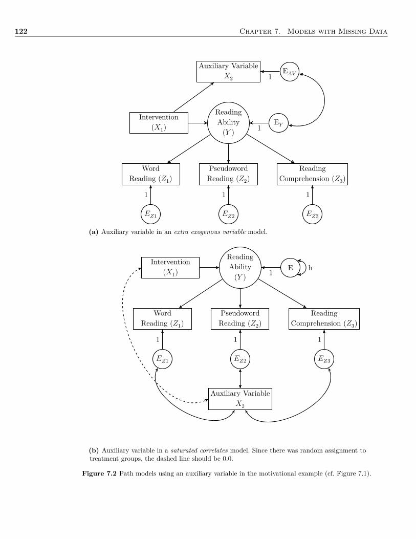
122 Chapter 7. Models with Missing Data
ReadingAbility(Y )
PseudowordReading (Z2)
WordReading (Z1)
ReadingComprehension (Z3)
EYIntervention
(X1) 1
EZ1 EZ2 EZ3
1 1 1
Auxiliary VariableX2
EAV1
(a) Auxiliary variable in an extra exogenous variable model.
ReadingAbility(Y )
PseudowordReading (Z2)
WordReading (Z1)
ReadingComprehension (Z3)
EIntervention
(X1) 1
EZ1 EZ2 EZ3
1 1 1
Auxiliary VariableX2
h
(b) Auxiliary variable in a saturated correlates model. Since there was random assignment totreatment groups, the dashed line should be 0.0.
Figure 7.2 Path models using an auxiliary variable in the motivational example (cf. Figure 7.1).
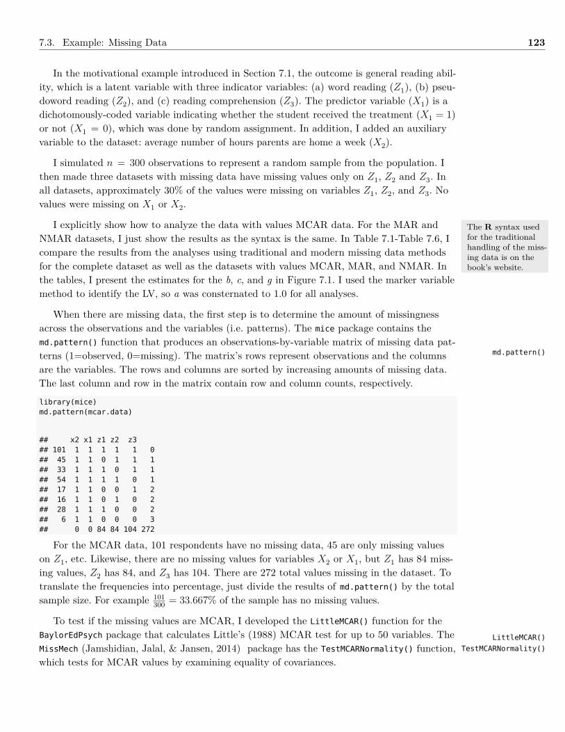
7.3. Example: Missing Data 123
In the motivational example introduced in Section 7.1, the outcome is general reading abil-ity, which is a latent variable with three indicator variables: (a) word reading (Z1), (b) pseu-doword reading (Z2), and (c) reading comprehension (Z3). The predictor variable (X1) is adichotomously-coded variable indicating whether the student received the treatment (X1 = 1)or not (X1 = 0), which was done by random assignment. In addition, I added an auxiliaryvariable to the dataset: average number of hours parents are home a week (X2).
I simulated n = 300 observations to represent a random sample from the population. Ithen made three datasets with missing data have missing values only on Z1, Z2 and Z3. Inall datasets, approximately 30% of the values were missing on variables Z1, Z2, and Z3. Novalues were missing on X1 or X2.
I explicitly show how to analyze the data with values MCAR data. For the MAR andNMAR datasets, I just show the results as the syntax is the same. In Table 7.1-Table 7.6, Icompare the results from the analyses using traditional and modern missing data methodsfor the complete dataset as well as the datasets with values MCAR, MAR, and NMAR. Inthe tables, I present the estimates for the b, c, and g in Figure 7.1. I used the marker variablemethod to identify the LV, so a was consternated to 1.0 for all analyses.
When there are missing data, the first step is to determine the amount of missingnessacross the observations and the variables (i.e. patterns). The mice package contains themd.pattern() function that produces an observations-by-variable matrix of missing data pat-terns (1=observed, 0=missing). The matrix’s rows represent observations and the columnsare the variables. The rows and columns are sorted by increasing amounts of missing data.The last column and row in the matrix contain row and column counts, respectively.
library(mice)md.pattern(mcar.data)
## x2 x1 z1 z2 z3## 101 1 1 1 1 1 0## 45 1 1 0 1 1 1## 33 1 1 1 0 1 1## 54 1 1 1 1 0 1## 17 1 1 0 0 1 2## 16 1 1 0 1 0 2## 28 1 1 1 0 0 2## 6 1 1 0 0 0 3## 0 0 84 84 104 272
For the MCAR data, 101 respondents have no missing data, 45 are only missing valueson Z1, etc. Likewise, there are no missing values for variables X2 or X1, but Z1 has 84 miss-ing values, Z2 has 84, and Z3 has 104. There are 272 total values missing in the dataset. Totranslate the frequencies into percentage, just divide the results of md.pattern() by the totalsample size. For example 101
300 = 33.667% of the sample has no missing values.
To test if the missing values are MCAR, I developed the LittleMCAR() function for theBaylorEdPsych package that calculates Little’s (1988) MCAR test for up to 50 variables. TheMissMech (Jamshidian, Jalal, & Jansen, 2014) package has the TestMCARNormality() function,which tests for MCAR values by examining equality of covariances.
The R syntax usedfor the traditionalhandling of the miss-ing data is on thebook’s website.
md.pattern()
LittleMCAR()
TestMCARNormality()
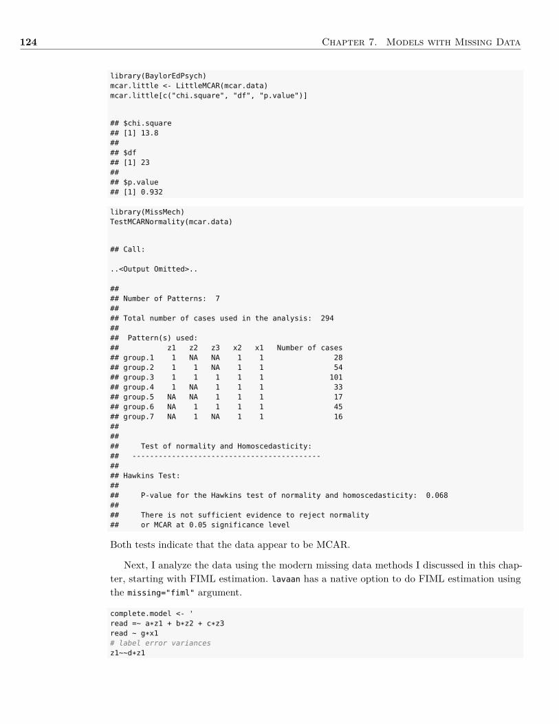
124 Chapter 7. Models with Missing Data
library(BaylorEdPsych)mcar.little <- LittleMCAR(mcar.data)mcar.little[c("chi.square", "df", "p.value")]
## $chi.square## [1] 13.8#### $df## [1] 23#### $p.value## [1] 0.932
library(MissMech)TestMCARNormality(mcar.data)
## Call:
..<Output Omitted>..
#### Number of Patterns: 7#### Total number of cases used in the analysis: 294#### Pattern(s) used:## z1 z2 z3 x2 x1 Number of cases## group.1 1 NA NA 1 1 28## group.2 1 1 NA 1 1 54## group.3 1 1 1 1 1 101## group.4 1 NA 1 1 1 33## group.5 NA NA 1 1 1 17## group.6 NA 1 1 1 1 45## group.7 NA 1 NA 1 1 16###### Test of normality and Homoscedasticity:## -------------------------------------------#### Hawkins Test:#### P-value for the Hawkins test of normality and homoscedasticity: 0.068#### There is not sufficient evidence to reject normality## or MCAR at 0.05 significance level
Both tests indicate that the data appear to be MCAR.
Next, I analyze the data using the modern missing data methods I discussed in this chap-ter, starting with FIML estimation. lavaan has a native option to do FIML estimation usingthe missing="fiml" argument.
complete.model <- 'read =~ a*z1 + b*z2 + c*z3read ~ g*x1# label error variancesz1~~d*z1
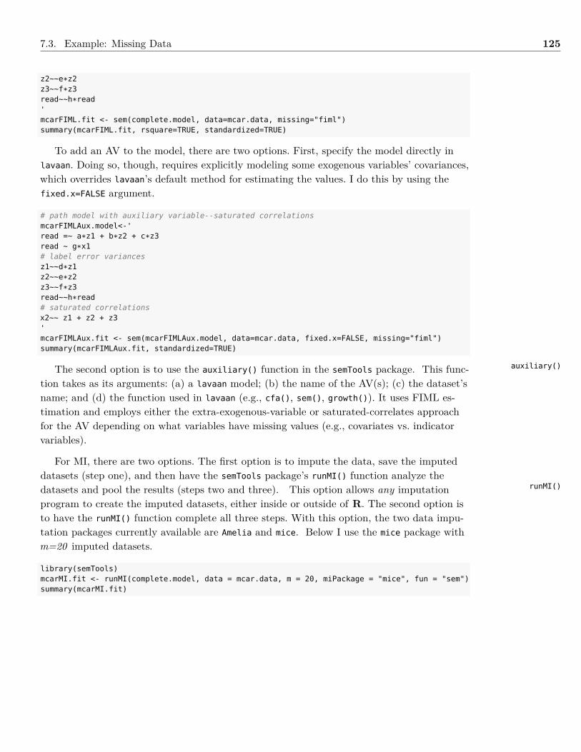
7.3. Example: Missing Data 125
z2~~e*z2z3~~f*z3read~~h*read'mcarFIML.fit <- sem(complete.model, data=mcar.data, missing="fiml")summary(mcarFIML.fit, rsquare=TRUE, standardized=TRUE)
To add an AV to the model, there are two options. First, specify the model directly inlavaan. Doing so, though, requires explicitly modeling some exogenous variables’ covariances,which overrides lavaan’s default method for estimating the values. I do this by using thefixed.x=FALSE argument.
# path model with auxiliary variable--saturated correlationsmcarFIMLAux.model<-'read =~ a*z1 + b*z2 + c*z3read ~ g*x1# label error variancesz1~~d*z1z2~~e*z2z3~~f*z3read~~h*read# saturated correlationsx2~~ z1 + z2 + z3'mcarFIMLAux.fit <- sem(mcarFIMLAux.model, data=mcar.data, fixed.x=FALSE, missing="fiml")summary(mcarFIMLAux.fit, standardized=TRUE)
The second option is to use the auxiliary() function in the semTools package. This func-tion takes as its arguments: (a) a lavaan model; (b) the name of the AV(s); (c) the dataset’sname; and (d) the function used in lavaan (e.g., cfa(), sem(), growth()). It uses FIML es-timation and employs either the extra-exogenous-variable or saturated-correlates approachfor the AV depending on what variables have missing values (e.g., covariates vs. indicatorvariables).
For MI, there are two options. The first option is to impute the data, save the imputeddatasets (step one), and then have the semTools package’s runMI() function analyze thedatasets and pool the results (steps two and three). This option allows any imputationprogram to create the imputed datasets, either inside or outside of R. The second option isto have the runMI() function complete all three steps. With this option, the two data impu-tation packages currently available are Amelia and mice. Below I use the mice package withm=20 imputed datasets.
library(semTools)mcarMI.fit <- runMI(complete.model, data = mcar.data, m = 20, miPackage = "mice", fun = "sem")summary(mcarMI.fit)
auxiliary()
runMI()
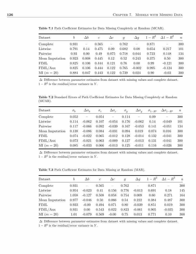
126 Chapter 7. Models with Missing Data
Table 7.1 Path Coefficient Estimates for Data Missing Completely at Random (MCAR).
Dataset b ∆b c ∆c g ∆g 1−R2 ∆1−R2 n
Complete 0.931 – 0.565 – 0.762 – 0.871 – 300Listwise 0.791 0.14 0.475 0.09 0.682 0.08 0.654 0.217 101Pairwise 0.93 0.00 0.49 0.075 0.718 0.044 0.723 0.148 134Mean Imputation 0.923 0.008 0.445 0.12 0.52 0.243 0.375 0.50 300FIML 0.825 0.106 0.444 0.121 0.76 0.00 0.99 -0.121 300FIML/Aux 0.825 0.106 0.444 0.122 0.765 -0.002 0.995 -0.124 300MI (m = 20) 0.884 0.047 0.443 0.122 0.739 0.024 0.90 -0.03 300
∆: Difference between parameter estimates from dataset with missing values and complete dataset.1−R2 is the residual/error variance in Y .
Table 7.2 Standard Errors of Path Coefficient Estimates for Data Missing Completely at Random(MCAR).
Dataset σb ∆σb σc ∆σc σg ∆σg σ1−R2 ∆σ1−R2 n
Complete 0.052 – 0.054 – 0.114 – 0.09 – 300Listwise 0.114 -0.062 0.107 -0.054 0.176 -0.062 0.14 -0.049 101Pairwise 0.117 -0.066 0.092 -0.039 0.167 -0.053 0.141 -0.051 134Mean Imputation 0.138 -0.086 0.084 -0.031 0.094 0.019 0.074 0.016 300FIML 0.074 -0.022 0.065 -0.012 0.128 -0.014 0.132 -0.041 300FIML/Aux 0.073 -0.021 0.063 -0.009 0.127 -0.013 0.131 -0.041 300MI (m = 20) 0.085 -0.033 0.066 -0.013 0.125 -0.011 0.116 -0.026 300
∆: Difference between parameter estimates from dataset with missing values and complete dataset.1−R2 is the residual/error variance in Y .
Table 7.3 Path Coefficient Estimates for Data Missing at Random (MAR).
Dataset b ∆b c ∆c g ∆g 1−R2 ∆1−R2 n
Complete 0.931 – 0.565 – 0.762 – 0.871 – 300Listwise 0.954 -0.023 0.41 0.156 0.776 -0.013 0.691 0.18 145Pairwise 1.058 -0.127 0.508 0.058 0.754 0.009 0.60 0.271 164Mean Imputation 0.977 -0.046 0.50 0.066 0.54 0.222 0.384 0.487 300FIML 0.933 -0.00 0.494 0.071 0.80 -0.039 0.851 0.019 300FIML/Aux 0.931 0.00 0.543 0.022 0.823 -0.061 0.905 -0.035 300MI (m = 20) 1.01 -0.079 0.569 -0.00 0.75 0.013 0.771 0.10 300
∆: Difference between parameter estimates from dataset with missing values and complete dataset.1−R2 is the residual/error variance in Y .
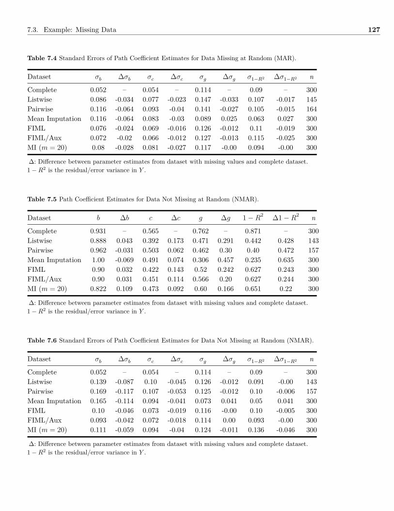
7.3. Example: Missing Data 127
Table 7.4 Standard Errors of Path Coefficient Estimates for Data Missing at Random (MAR).
Dataset σb ∆σb σc ∆σc σg ∆σg σ1−R2 ∆σ1−R2 n
Complete 0.052 – 0.054 – 0.114 – 0.09 – 300Listwise 0.086 -0.034 0.077 -0.023 0.147 -0.033 0.107 -0.017 145Pairwise 0.116 -0.064 0.093 -0.04 0.141 -0.027 0.105 -0.015 164Mean Imputation 0.116 -0.064 0.083 -0.03 0.089 0.025 0.063 0.027 300FIML 0.076 -0.024 0.069 -0.016 0.126 -0.012 0.11 -0.019 300FIML/Aux 0.072 -0.02 0.066 -0.012 0.127 -0.013 0.115 -0.025 300MI (m = 20) 0.08 -0.028 0.081 -0.027 0.117 -0.00 0.094 -0.00 300
∆: Difference between parameter estimates from dataset with missing values and complete dataset.1−R2 is the residual/error variance in Y .
Table 7.5 Path Coefficient Estimates for Data Not Missing at Random (NMAR).
Dataset b ∆b c ∆c g ∆g 1−R2 ∆1−R2 n
Complete 0.931 – 0.565 – 0.762 – 0.871 – 300Listwise 0.888 0.043 0.392 0.173 0.471 0.291 0.442 0.428 143Pairwise 0.962 -0.031 0.503 0.062 0.462 0.30 0.40 0.472 157Mean Imputation 1.00 -0.069 0.491 0.074 0.306 0.457 0.235 0.635 300FIML 0.90 0.032 0.422 0.143 0.52 0.242 0.627 0.243 300FIML/Aux 0.90 0.031 0.451 0.114 0.566 0.20 0.627 0.244 300MI (m = 20) 0.822 0.109 0.473 0.092 0.60 0.166 0.651 0.22 300
∆: Difference between parameter estimates from dataset with missing values and complete dataset.1−R2 is the residual/error variance in Y .
Table 7.6 Standard Errors of Path Coefficient Estimates for Data Not Missing at Random (NMAR).
Dataset σb ∆σb σc ∆σc σg ∆σg σ1−R2 ∆σ1−R2 n
Complete 0.052 – 0.054 – 0.114 – 0.09 – 300Listwise 0.139 -0.087 0.10 -0.045 0.126 -0.012 0.091 -0.00 143Pairwise 0.169 -0.117 0.107 -0.053 0.125 -0.012 0.10 -0.006 157Mean Imputation 0.165 -0.114 0.094 -0.041 0.073 0.041 0.05 0.041 300FIML 0.10 -0.046 0.073 -0.019 0.116 -0.00 0.10 -0.005 300FIML/Aux 0.093 -0.042 0.072 -0.018 0.114 0.00 0.093 -0.00 300MI (m = 20) 0.111 -0.059 0.094 -0.04 0.124 -0.011 0.136 -0.046 300
∆: Difference between parameter estimates from dataset with missing values and complete dataset.1−R2 is the residual/error variance in Y .
128 Chapter 7. Models with Missing Data
7.4 SummaryIn this chapter I discussed three types of missing data: missing completely at random, miss-ing at random, and not missing at random. In addition, I discussed why traditional methodsfor handling missing data might not work and showed how to implement two more robustmethods: full-information maximum likelihood and multiple imputation. Moreover, I intro-duced auxiliary variables and showed how they can be added to a path model to improveparameter estimation accuracy when there are missing data. I finished the chapter by explic-itly working through a example in R using a dataset with missing values.
7.5 Writing the ResultsA major component of any data analysis should be to check to see if there are any missingdata. This is relatively easy to do with the mice package’s md.pattern() function as I demon-strated in Section 7.3. If there are missing values, Schlomer, Bauman, and Card (2010) sug-gest three imperatives when reporting the analysis results:
1. Report the amount of missing data.2. Report the types of missing data (or at least the likely missing data types).3. Report on how the most appropriate method for handling missing data was deter-
mined.
When reporting the amount of missing data, give the percentage of missing data, either inthe text (e.g., “Missing data ranged from a low of 2% for Reading Comprehension to a highof 10% for Word Reading”) or in a table along with other descriptive statistics. If the studyinvolves multiple time periods report the percentage of attrition and missing data at eachtime period as well as over the entire study.
To examine the type of missing data, use Little’s (1988) test to assess means and the testdeveloped by Jamshidian et al. (2014) to assess covariances. Although neither test has beenstudied in great depth, hopefully they converge in their results. If they do not converge, or ifboth tests indicate the missing values are not MCAR, use univariate methods to see if thereare particular variables that strongly violate the MCAR assumptions. Be sure to include aconclusion about the types of missing data patterns in the Results section after reporting theamount of missing data.
When determining the most appropriate method to handle missing data, the defaultchoice should be using FIML or MI (with auxiliary variables, if possible), unless you canmake an argument that another method is better for a specific situation. If you chose anothermethod, be explicit in your rationale for choosing it and state why it is better than eitherFIML or MI.
7.6 Exercises7.1 The complete, MCAR, MAR, and NMAR data are on the book’s website.
7.1.a Import the three datasets with missing values into R and name them mcar.data,mar.data, and nmar.data, respectively.
7.1.b Test to see if the missing data is MCAR.
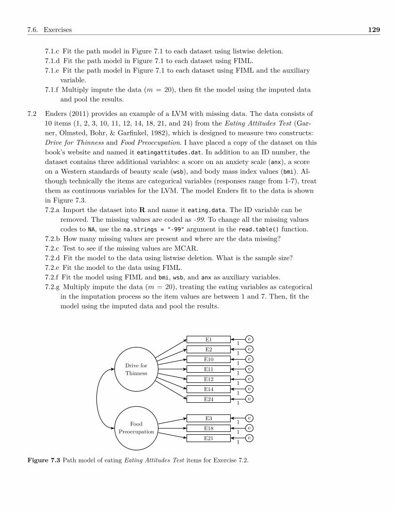
7.6. Exercises 129
7.1.c Fit the path model in Figure 7.1 to each dataset using listwise deletion.7.1.d Fit the path model in Figure 7.1 to each dataset using FIML.7.1.e Fit the path model in Figure 7.1 to each dataset using FIML and the auxiliary
variable.7.1.f Multiply impute the data (m = 20), then fit the model using the imputed data
and pool the results.
7.2 Enders (2011) provides an example of a LVM with missing data. The data consists of10 items (1, 2, 3, 10, 11, 12, 14, 18, 21, and 24) from the Eating Attitudes Test (Gar-ner, Olmsted, Bohr, & Garfinkel, 1982), which is designed to measure two constructs:Drive for Thinness and Food Preoccupation. I have placed a copy of the dataset on thisbook’s website and named it eatingattitudes.dat. In addition to an ID number, thedataset contains three additional variables: a score on an anxiety scale (anx), a scoreon a Western standards of beauty scale (wsb), and body mass index values (bmi). Al-though technically the items are categorical variables (responses range from 1-7), treatthem as continuous variables for the LVM. The model Enders fit to the data is shownin Figure 7.3.7.2.a Import the dataset into R and name it eating.data. The ID variable can be
removed. The missing values are coded as -99. To change all the missing valuescodes to NA, use the na.strings = "-99" argument in the read.table() function.
7.2.b How many missing values are present and where are the data missing?7.2.c Test to see if the missing values are MCAR.7.2.d Fit the model to the data using listwise deletion. What is the sample size?7.2.e Fit the model to the data using FIML.7.2.f Fit the model using FIML and bmi, wsb, and anx as auxiliary variables.7.2.g Multiply impute the data (m = 20), treating the eating variables as categorical
in the imputation process so the item values are between 1 and 7. Then, fit themodel using the imputed data and pool the results.
Drive forThinness
FoodPreoccupation
E11
E10
E2
E1
E12
E14
E24
E18
E3
E21
e
e
e
e
e
e
e
e
e
e
1
1
1
1
1
1
1
1
1
1
Figure 7.3 Path model of eating Eating Attitudes Test items for Exercise 7.2.
130 Chapter 7. Models with Missing Data
7.7 References & Further ReadingsEnders, C. K. (2005). Maximum likelihood estimation. In B. Everitt & D. C. Howell (Eds.),
Encyclopedia of behavioral statistics (pp. 1164–1170). West Sussex, England: Wiley.Enders, C. K. (2011). Applied missing data analysis. New York, NY: Guilford.Garner, D. M., Olmsted, M. P., Bohr, Y., & Garfinkel, P. E. (1982). The Eating Attitudes
Test: Psychometric features and clinical correlates. Psychological Medicine, 12 , 871-878.Graham, J. W. (2003). Adding missing-data-relevant variables to FIML-based structural
equation models. Structural Equation Modeling: A Multidisciplinary Journal, 10 ,80-100. doi: 10.1207/S15328007SEM1001_4
Graham, J. W. (2009). Missing data analysis: Making it work in the real world. AnnualReview of Psychology, 60 , 549-576. doi: 10.1146/annurev.psych.58.110405.085530
Jamshidian, M., & Jalal, S. (2010). Tests of homoscedasticity, normality, and missingcompletely at random for incomplete multivariate data. Psychometrika, 75 . doi:10.1007/s11336-010-9175-3
Jamshidian, M., Jalal, S., & Jansen, C. (2014). MissMech: An R package for testinghomoscedasticity, multivariate normality, and missing completely at random (MCAR).Journal of Statistical Software, 56 (6), 1-30. Retrieved fromhttp://www.jstatsoft.org/v56/i06.
Little, R. J. A. (1988). A test of missing completely at random for multivariate data withmissing values. Journal of the American Statistical Association, 83 , 1198-1202.
Little, R. J. A., & Rubin, D. B. (2002). Statistical analysis with missing data (2nd ed.).Hoboken, NJ: John Wiley.
Lottes, I. L., DeMaris, A., & Adler, M. A. (1996). Using and interpreting logistic regression: Aguide for teachers and students. Teaching Sociology, 24 , 284-298.
McArdle, J. J. (1994). Structural factor analysis experiments with incomplete data.Multivariate Behavioral Research, 29 , 409-454. doi: 10.1207/s15327906mbr2904_5
Muthén, B. O., Asparouhov, T., Hunter, A. M., & Leuchter, A. F. (2011). Growth modelingwith nonignorable dropout: Alternative analyses of the STAR*D antidepressant trial.Psychological Methods, 16 , 17-33. doi: 10.1037/a0022634
Schafer, J. L., & Graham, J. W. (2002). Missing data: Our view of the state of the art.Psychological Methods, 7 , 147-177. doi: 10.1037/1082-989X.7.2.147
Schlomer, G. L., Bauman, S., & Card, N. A. (2010). Best practices for missing datamanagement in counseling psychology. Journal of Counseling Psychology, 57 , 1-10. doi:10.1037/a0018082
van Buuren, S., & Groothuis-Oudshoorn, K. (2011). Multivariate imputation by chainedequations in R. Journal of Statistical Software, 45 (3). Retrieved fromhttp://www.jstatsoft.org/v45/i03/.
Wilkinson, L., & American Psychological Association Science Directorate Task Force onStatistical Inference. (1999). Statistical methods in psychology journals: Guidelines andexplanations. American Psychologist, 54 , 594-604. doi: 10.1037/0003-066X.54.8.594
8 | Sample Size Planning
Chapter Contents8.1 Background . . . . . . . . . . . . . . . . . . . . . . . . . . . . . . . . . . . . 131
8.1.1 Traditional Sample Size Determination . . . . . . . . . . . . . . . . . 1318.1.2 Determining Sample Size Through a Monte Carlo Study . . . . . . . 1338.1.3 Example: Sample Size for a Simple Regression Model . . . . . . . . . 1348.1.4 Example: Sample Size for a Latent Variable Model . . . . . . . . . . 137
8.2 Summary . . . . . . . . . . . . . . . . . . . . . . . . . . . . . . . . . . . . . . 1428.3 Writing the Results . . . . . . . . . . . . . . . . . . . . . . . . . . . . . . . . 1428.4 Exercises . . . . . . . . . . . . . . . . . . . . . . . . . . . . . . . . . . . . . . 1438.5 References & Further Readings . . . . . . . . . . . . . . . . . . . . . . . . . . 144
8.1 BackgroundWhen designing a study, whether using a LVM or not, it is important to consider the sam-ple size needed for the analysis. Required for what?, you might ask. Usually it is the samplesize required to reject a false null hypothesis (H0) for a given effect size.1 This idea stemsfrom null hypothesis significance testing (NHST). NHST, at least how it is currently imple-mented, pits two competing hypotheses against each other. H0 is usually set up to be theantithesis of the hypothesis of interest. Conversely, the alternative hypothesis (Ha or H1) isevery hypothesis that is not H0. Often, H0 is specified such that a parameter is equal to avalue (e.g., H0 : δ = 0), which makes Ha be that the parameter is not equal to the value (e.g.,Ha : δ 6= 0).
There are four interrelated concepts when determining the needed sample size: (a) type 1error; (b) type 2 error; (c) sample size; and (d) effect size. Type 1 error (α) is the frequencyof rejecting a true H0, based on multiple data samples from the same population. Thus, whenα is large, I will frequently say my data indicate there is an effect, when one is not presentin the population (i.e., large false + rate). Conversely, type 2 error (β) is the frequency ofaccepting a false H0, based on multiple data samples from the same population. When β islarge, I will often conclude that my data indicate there is not an effect when one is present inthe population (i.e., large false - rate). Statistical power is defined in terms of β: it is 1− β.That is, across the multiple samples, power is the frequency I will say the results indicatethere is an effect, when there is one in the population.
8.1.1 Traditional Sample Size DeterminationAs an example, say I want to determine if the entrance exam scores for the 2012-2013 enter-ing class at a university are different than the scores from the 2011-2012 entering class. Thenull and alternative hypotheses are:
β is used to indicatetype 2 error and,sometimes, the pop-ulation version ofa path coefficient(see Section 2.1.5).The meanings areindependent andshould not be usedinterchangeably.
Power
1Kelley and Maxwell (2012) provide an alternative reason for determining sample size: precision of parame-ter estimates. The methods presented in this chapter can be used for purposes. Since a focus on power is morecommon when determining sample size, that is the focus I use throughout this chapter.
131
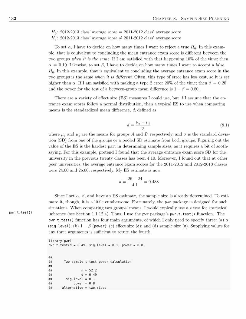
132 Chapter 8. Sample Size Planning
pwr.t.test()
H0: 2012-2013 class’ average score = 2011-2012 class’ average scoreHa: 2012-2013 class’ average score 6= 2011-2012 class’ average score
To set α, I have to decide on how many times I want to reject a true H0. In this exam-ple, that is equivalent to concluding the mean entrance exam score is different between thetwo groups when it is the same. If I am satisfied with that happening 10% of the time; thenα = 0.10. Likewise, to set β, I have to decide on how many times I want to accept a falseH0. In this example, that is equivalent to concluding the average entrance exam score in thetwo groups is the same when it is different. Often, this type of error has less cost, so it is sethigher than α. If I am satisfied with making a type 2 error 20% of the time; then β = 0.20and the power for the test of a between-group mean difference is 1− β = 0.80.
There are a variety of effect size (ES) measures I could use, but if I assume that the en-trance exam scores follow a normal distribution, then a typical ES to use when comparingmeans is the standardized mean difference, d, defined as
d = µa − µbσ
(8.1)
where µa and µb are the means for groups A and B, respectively, and σ is the standard devia-tion (SD) from one of the groups or a pooled SD estimate from both groups. Figuring out thevalue of the ES is the hardest part in determining sample sizes, as it requires a bit of sooth-saying. For this example, pretend I found that the average entrance exam score SD for theuniversity in the previous twenty classes has been 4.10. Moreover, I found out that at otherpeer universities, the average entrance exam scores for the 2011-2012 and 2012-2013 classeswere 24.00 and 26.00, respectively. My ES estimate is now:
d = 26− 244.1 = 0.488
Since I set α, β, and have an ES estimate, the sample size is already determined. To esti-mate it, though, it is a little cumbersome. Fortunately, the pwr package is designed for suchsituations. When comparing two groups’ means, I would typically use a t test for statisticalinference (see Section 1.1.12.4). Thus, I use the pwr package’s pwr.t.test() function. Thepwr.t.test() function has four main arguments, of which I only need to specify three: (a) α(sig.level); (b) 1− β (power); (c) effect size (d); and (d) sample size (n). Supplying values forany three arguments is sufficient to return the fourth.
library(pwr)pwr.t.test(d = 0.49, sig.level = 0.1, power = 0.8)
#### Two-sample t test power calculation#### n = 52.2## d = 0.49## sig.level = 0.1## power = 0.8## alternative = two.sided
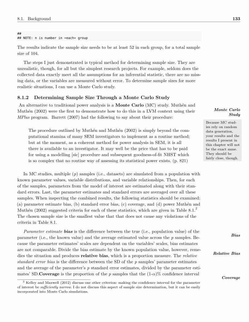
8.1. Background 133
#### NOTE: n is number in *each* group
The results indicate the sample size needs to be at least 52 in each group, for a total samplesize of 104.
The steps I just demonstrated is typical method for determining sample size. They areunrealistic, though, for all but the simplest research projects. For example, seldom does thecollected data exactly meet all the assumptions for an inferential statistic, there are no miss-ing data, or the variables are measured without error. To determine sample sizes for morerealistic situations, I can use a Monte Carlo study.
8.1.2 Determining Sample Size Through a Monte Carlo StudyAn alternative to traditional power analysis is a Monte Carlo (MC) study. Muthén andMuthén (2002) were the first to demonstrate how to do this in a LVM context using theirMPlus program. Barrett (2007) had the following to say about their procedure:
The procedure outlined by Muthén and Muthén (2002) is simply beyond the com-putational stamina of many SEM investigators to implement as a routine method;but at the moment, as a coherent method for power analysis in SEM, it is allthere is available to an investigator. It may well be the price that has to be paidfor using a modelling [sic] procedure and subsequent goodness-of-fit NHST whichis so complex that no routine way of assessing its statistical power exists. (p. 821)
In MC studies, multiple (p) samples (i.e., datasets) are simulated from a population withknown parameter values, variable distributions, and variable relationships. Then, for eachof the samples, parameters from the model of interest are estimated along with their stan-dard errors. Last, the parameter estimates and standard errors are averaged over all thesesamples. When inspecting the combined results, the following statistics should be examined:(a) parameter estimate bias, (b) standard error bias, (c) coverage, and (d) power Muthén andMuthén (2002) suggested criteria for each of these statistics, which are given in Table 8.1.2
The chosen sample size is the smallest value that that does not cause any violations of thecriteria in Table 8.1.
Parameter estimate bias is the difference between the true (i.e., population value) of theparameter (i.e., the known value) and the average estimated value across the p samples. Be-cause the parameter estimates’ scales are dependent on the variables’ scales, bias estimatesare not comparable. Divide the bias estimate by the known population value, however, reme-dies the situation and produces relative bias, which is a proportion measure. The relativestandard error bias is the difference between the SD of the p samples’ parameter estimatesand the average of the parameter’s p standard error estimates, divided by the parameter esti-mates’ SD.Coverage is the proportion of the p samples that the (1-α)% confidence interval
Monte CarloStudy
Because MC stud-ies rely on randomdata generation,your results and theresults I present inthis chapter will notbe the exact same.They should befairly close, though.
Bias
Relative Bias
Coverage2 Kelley and Maxwell (2012) discuss one other criterion: making the confidence interval for the parameter
of interest be sufficiently narrow. I do not discuss this aspect of sample size determination, but it can be easilyincorporated into Monte Carlo simulations.
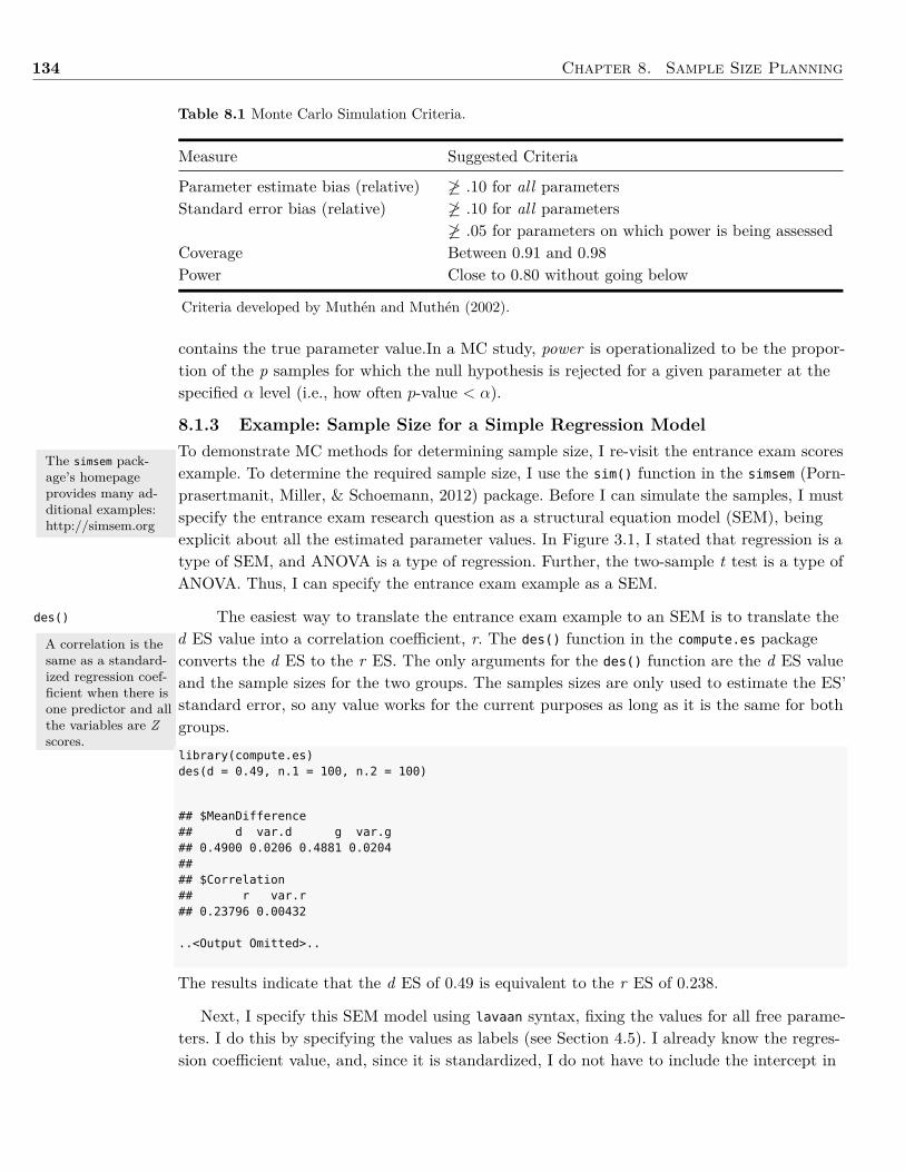
134 Chapter 8. Sample Size Planning
Table 8.1 Monte Carlo Simulation Criteria.
Measure Suggested Criteria
Parameter estimate bias (relative) 6≥ .10 for all parametersStandard error bias (relative) 6≥ .10 for all parameters
6≥ .05 for parameters on which power is being assessedCoverage Between 0.91 and 0.98Power Close to 0.80 without going below
Criteria developed by Muthén and Muthén (2002).
The simsem pack-age’s homepageprovides many ad-ditional examples:http://simsem.org
des()
A correlation is thesame as a standard-ized regression coef-ficient when there isone predictor and allthe variables are Zscores.
contains the true parameter value.In a MC study, power is operationalized to be the propor-tion of the p samples for which the null hypothesis is rejected for a given parameter at thespecified α level (i.e., how often p-value < α).
8.1.3 Example: Sample Size for a Simple Regression ModelTo demonstrate MC methods for determining sample size, I re-visit the entrance exam scoresexample. To determine the required sample size, I use the sim() function in the simsem (Porn-prasertmanit, Miller, & Schoemann, 2012) package. Before I can simulate the samples, I mustspecify the entrance exam research question as a structural equation model (SEM), beingexplicit about all the estimated parameter values. In Figure 3.1, I stated that regression is atype of SEM, and ANOVA is a type of regression. Further, the two-sample t test is a type ofANOVA. Thus, I can specify the entrance exam example as a SEM.
The easiest way to translate the entrance exam example to an SEM is to translate thed ES value into a correlation coefficient, r. The des() function in the compute.es packageconverts the d ES to the r ES. The only arguments for the des() function are the d ES valueand the sample sizes for the two groups. The samples sizes are only used to estimate the ES’standard error, so any value works for the current purposes as long as it is the same for bothgroups.library(compute.es)des(d = 0.49, n.1 = 100, n.2 = 100)
## $MeanDifference## d var.d g var.g## 0.4900 0.0206 0.4881 0.0204#### $Correlation## r var.r## 0.23796 0.00432
..<Output Omitted>..
The results indicate that the d ES of 0.49 is equivalent to the r ES of 0.238.
Next, I specify this SEM model using lavaan syntax, fixing the values for all free parame-ters. I do this by specifying the values as labels (see Section 4.5). I already know the regres-sion coefficient value, and, since it is standardized, I do not have to include the intercept in
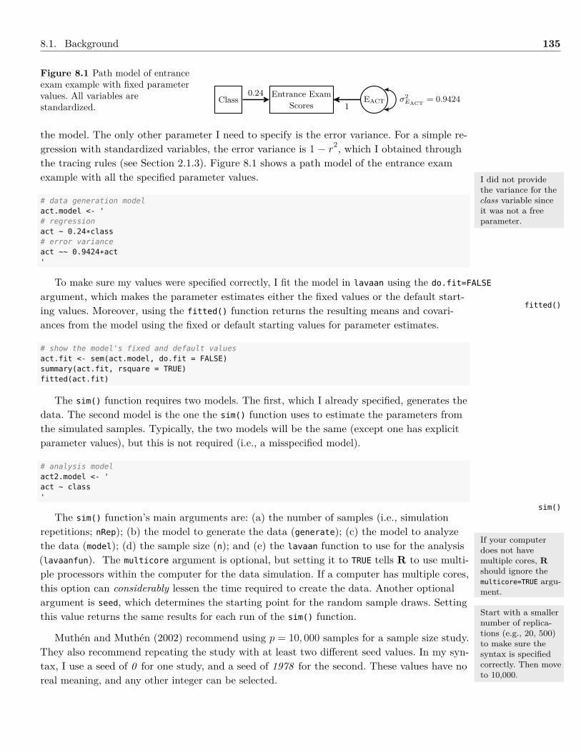
8.1. Background 135
Figure 8.1 Path model of entranceexam example with fixed parametervalues. All variables arestandardized.
Class Entrance ExamScores
EACT σ2EACT = 0.9424
0.241
the model. The only other parameter I need to specify is the error variance. For a simple re-gression with standardized variables, the error variance is 1 − r2, which I obtained throughthe tracing rules (see Section 2.1.3). Figure 8.1 shows a path model of the entrance examexample with all the specified parameter values.
# data generation modelact.model <- '# regressionact ~ 0.24*class# error varianceact ~~ 0.9424*act'
To make sure my values were specified correctly, I fit the model in lavaan using the do.fit=FALSE
argument, which makes the parameter estimates either the fixed values or the default start-ing values. Moreover, using the fitted() function returns the resulting means and covari-ances from the model using the fixed or default starting values for parameter estimates.
# show the model's fixed and default valuesact.fit <- sem(act.model, do.fit = FALSE)summary(act.fit, rsquare = TRUE)fitted(act.fit)
The sim() function requires two models. The first, which I already specified, generates thedata. The second model is the one the sim() function uses to estimate the parameters fromthe simulated samples. Typically, the two models will be the same (except one has explicitparameter values), but this is not required (i.e., a misspecified model).
# analysis modelact2.model <- 'act ~ class'
The sim() function’s main arguments are: (a) the number of samples (i.e., simulationrepetitions; nRep); (b) the model to generate the data (generate); (c) the model to analyzethe data (model); (d) the sample size (n); and (e) the lavaan function to use for the analysis(lavaanfun). The multicore argument is optional, but setting it to TRUE tells R to use multi-ple processors within the computer for the data simulation. If a computer has multiple cores,this option can considerably lessen the time required to create the data. Another optionalargument is seed, which determines the starting point for the random sample draws. Settingthis value returns the same results for each run of the sim() function.
Muthén and Muthén (2002) recommend using p = 10, 000 samples for a sample size study.They also recommend repeating the study with at least two different seed values. In my syn-tax, I use a seed of 0 for one study, and a seed of 1978 for the second. These values have noreal meaning, and any other integer can be selected.
I did not providethe variance for theclass variable sinceit was not a freeparameter.
fitted()
sim()
If your computerdoes not havemultiple cores, Rshould ignore themulticore=TRUE argu-ment.
Start with a smallernumber of replica-tions (e.g., 20, 500)to make sure thesyntax is specifiedcorrectly. Then moveto 10,000.
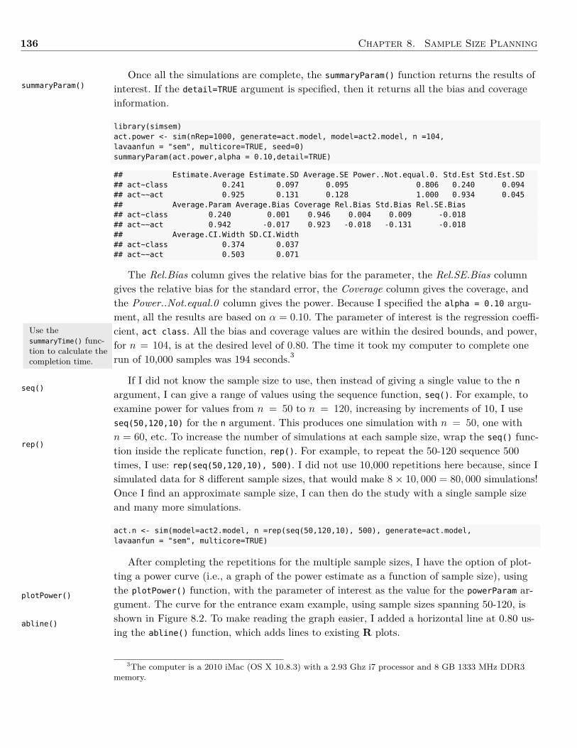
136 Chapter 8. Sample Size Planning
summaryParam()
Use thesummaryTime() func-tion to calculate thecompletion time.
seq()
rep()
plotPower()
abline()
Once all the simulations are complete, the summaryParam() function returns the results ofinterest. If the detail=TRUE argument is specified, then it returns all the bias and coverageinformation.
library(simsem)act.power <- sim(nRep=1000, generate=act.model, model=act2.model, n =104,lavaanfun = "sem", multicore=TRUE, seed=0)summaryParam(act.power,alpha = 0.10,detail=TRUE)
## Estimate.Average Estimate.SD Average.SE Power..Not.equal.0. Std.Est Std.Est.SD## act~class 0.241 0.097 0.095 0.806 0.240 0.094## act~~act 0.925 0.131 0.128 1.000 0.934 0.045## Average.Param Average.Bias Coverage Rel.Bias Std.Bias Rel.SE.Bias## act~class 0.240 0.001 0.946 0.004 0.009 -0.018## act~~act 0.942 -0.017 0.923 -0.018 -0.131 -0.018## Average.CI.Width SD.CI.Width## act~class 0.374 0.037## act~~act 0.503 0.071
The Rel.Bias column gives the relative bias for the parameter, the Rel.SE.Bias columngives the relative bias for the standard error, the Coverage column gives the coverage, andthe Power..Not.equal.0 column gives the power. Because I specified the alpha = 0.10 argu-ment, all the results are based on α = 0.10. The parameter of interest is the regression coeffi-cient, act class. All the bias and coverage values are within the desired bounds, and power,for n = 104, is at the desired level of 0.80. The time it took my computer to complete onerun of 10,000 samples was 194 seconds.3
If I did not know the sample size to use, then instead of giving a single value to the n
argument, I can give a range of values using the sequence function, seq(). For example, toexamine power for values from n = 50 to n = 120, increasing by increments of 10, I useseq(50,120,10) for the n argument. This produces one simulation with n = 50, one withn = 60, etc. To increase the number of simulations at each sample size, wrap the seq() func-tion inside the replicate function, rep(). For example, to repeat the 50-120 sequence 500times, I use: rep(seq(50,120,10), 500). I did not use 10,000 repetitions here because, since Isimulated data for 8 different sample sizes, that would make 8× 10, 000 = 80, 000 simulations!Once I find an approximate sample size, I can then do the study with a single sample sizeand many more simulations.
act.n <- sim(model=act2.model, n =rep(seq(50,120,10), 500), generate=act.model,lavaanfun = "sem", multicore=TRUE)
After completing the repetitions for the multiple sample sizes, I have the option of plot-ting a power curve (i.e., a graph of the power estimate as a function of sample size), usingthe plotPower() function, with the parameter of interest as the value for the powerParam ar-gument. The curve for the entrance exam example, using sample sizes spanning 50-120, isshown in Figure 8.2. To make reading the graph easier, I added a horizontal line at 0.80 us-ing the abline() function, which adds lines to existing R plots.
3The computer is a 2010 iMac (OS X 10.8.3) with a 2.93 Ghz i7 processor and 8 GB 1333 MHz DDR3memory.
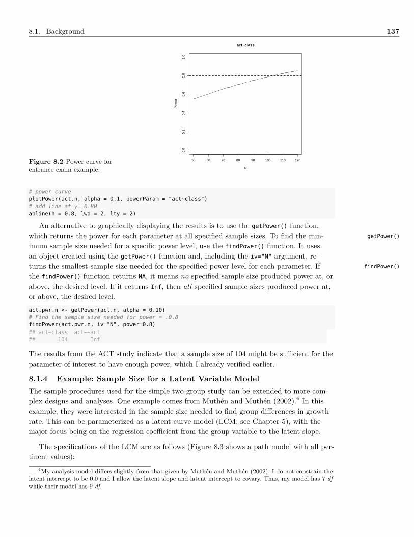
8.1. Background 137
Figure 8.2 Power curve forentrance exam example.
50 60 70 80 90 100 110 120
0.0
0.2
0.4
0.6
0.8
1.0
act~class
N
Pow
er
# power curveplotPower(act.n, alpha = 0.1, powerParam = "act~class")# add line at y= 0.80abline(h = 0.8, lwd = 2, lty = 2)
An alternative to graphically displaying the results is to use the getPower() function,which returns the power for each parameter at all specified sample sizes. To find the min-imum sample size needed for a specific power level, use the findPower() function. It usesan object created using the getPower() function and, including the iv="N" argument, re-turns the smallest sample size needed for the specified power level for each parameter. Ifthe findPower() function returns NA, it means no specified sample size produced power at, orabove, the desired level. If it returns Inf, then all specified sample sizes produced power at,or above, the desired level.
act.pwr.n <- getPower(act.n, alpha = 0.10)# Find the sample size needed for power = .0.8findPower(act.pwr.n, iv="N", power=0.8)## act~class act~~act## 104 Inf
The results from the ACT study indicate that a sample size of 104 might be sufficient for theparameter of interest to have enough power, which I already verified earlier.
8.1.4 Example: Sample Size for a Latent Variable ModelThe sample procedures used for the simple two-group study can be extended to more com-plex designs and analyses. One example comes from Muthén and Muthén (2002).4 In thisexample, they were interested in the sample size needed to find group differences in growthrate. This can be parameterized as a latent curve model (LCM; see Chapter 5), with themajor focus being on the regression coefficient from the group variable to the latent slope.
The specifications of the LCM are as follows (Figure 8.3 shows a path model with all per-tinent values):
getPower()
findPower()
4My analysis model differs slightly from that given by Muthén and Muthén (2002). I do not constrain thelatent intercept to be 0.0 and I allow the latent slope and latent intercept to covary. Thus, my model has 7 dfwhile their model has 9 df.
138 Chapter 8. Sample Size Planning
• Four equidistant time periods measuring the same continuous variable (Y1 − Y4) that isnormally distributed.
• There is a covariate representing group membership (X). Group membership is dummycoded (0=no, 1=yes), and there are equal numbers of both groups. Thus, the mean andvariance of X are 0.50 and 0.25, respectively.
• The mean of the latent intercept and latent slope are 0.00 and 0.20, respectively.• The latent mean and latent slope covariance is 0.00.• The residual variances for the indicator variables are all 0.50.• The regression coefficient for the latent intercept is 0.50, with a residual variance of
0.25.• The residual variance for the latent slope is 0.09.• α = 0.05 and the desired power is 0.80• The regression coefficient for the latent slope is 0.20, which is the same as having a d
ES of 0.63.
The ES calculation is a straightforward application of the tracing rules. The between-group difference in latent slopes is 0.20. The latent slope variance is 0.20× 0.25× 0.20 + 1×0.09× 1 = 0.10. Thus, using Equation (8.1), I get:
d = 0.20√0.10
= 0.63
The procedure to find a sample size for the LCM follows that from the entrance examexample. I have to specify a data generation model and a data analysis model. Since thereare many more parameters in this mode, I labeled the parameter of interest as a. For thislabeling to work, I have to do it in both the generation and analysis models. To check theparameter values, I use the do.fit=FALSE argument in lavaan with the data generation model.Because I explicitly constrained the means and variances of an exogenous variable (X), Ineed to include the fixed.x=FALSE argument as well.
# Data generation modellcm.pop.model <- '# latent variable modeli =~ 1*y1 + 1*y2 + 1*y3 + 1*y4s =~ 0*y1 + 1*y2 + 2*y3 + 3*y4# latent variable meansi ~ 0.00*1s ~ 0.20*1# regressions, with parameter of interest labeledi ~ 0.50*xs ~ a*x + 0.20*x# mean and variance of xx ~ 0.50*1x ~~ 0.25*x# manifest (residual) variancesy1 ~~ 0.5*y1y2 ~~ 0.5*y2y3 ~~ 0.5*y3y4 ~~ 0.5*y4# latent variable residual variances/covariances
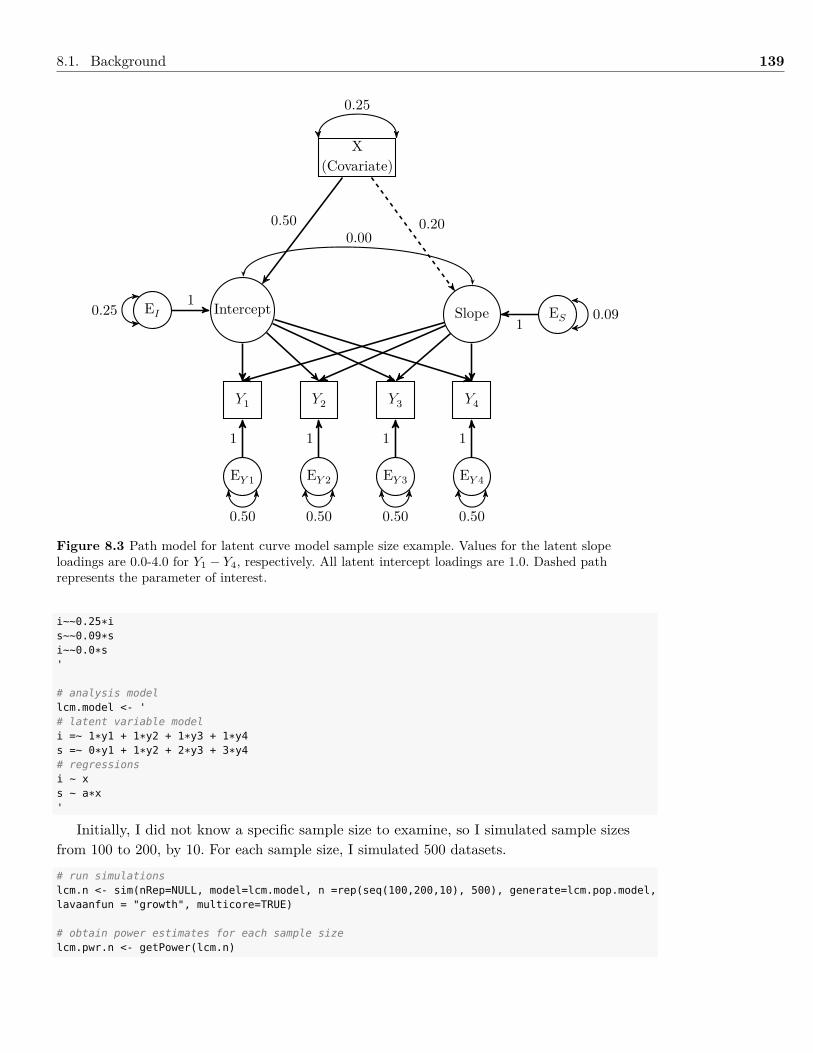
8.1. Background 139
Y1 Y2 Y3 Y4
Intercept Slope
X(Covariate)
EI ES1
10.25 0.09
0.000.50 0.20
EY 1 EY 2 EY 3 EY 4
1 1 1 1
0.50 0.50 0.50 0.50
0.25
Figure 8.3 Path model for latent curve model sample size example. Values for the latent slopeloadings are 0.0-4.0 for Y1 − Y4, respectively. All latent intercept loadings are 1.0. Dashed pathrepresents the parameter of interest.
i~~0.25*is~~0.09*si~~0.0*s'
# analysis modellcm.model <- '# latent variable modeli =~ 1*y1 + 1*y2 + 1*y3 + 1*y4s =~ 0*y1 + 1*y2 + 2*y3 + 3*y4# regressionsi ~ xs ~ a*x'
Initially, I did not know a specific sample size to examine, so I simulated sample sizesfrom 100 to 200, by 10. For each sample size, I simulated 500 datasets.
# run simulationslcm.n <- sim(nRep=NULL, model=lcm.model, n =rep(seq(100,200,10), 500), generate=lcm.pop.model,lavaanfun = "growth", multicore=TRUE)
# obtain power estimates for each sample sizelcm.pwr.n <- getPower(lcm.n)
140 Chapter 8. Sample Size Planning
miss()
# find the sample size needed for power = .0.8findPower(lcm.pwr.n, "N", 0.8)## i~x a y1~~y1 y2~~y2 y3~~y3 y4~~y4 i~~i s~~s i~~s i~1 s~1## 100 149 100 Inf Inf 100 135 100 NA NA 100
It appears that a sample size of 149 should be adequate for this model.
I checked this sample size of 149 by redoing the study using 10,000 repetitions. I did thistwice, each with a different seed value. The bias and coverage values were all within the speci-fied limits, and power was 0.80. For space considerations, I only show results from one of thestudies.lcm1.power <- sim(nRep=10000, model=lcm.model, n =149, generate=lcm.pop.model,lavaanfun = "growth", multicore=TRUE, seed=998877)lcm2.power <- sim(nRep=10000, model=lcm.model, n =149, generate=lcm.pop1.model,lavaanfun = "growth", multicore=TRUE, seed=99)summaryParam(lcm1.power,alpha = 0.05,detail=TRUE)summaryParam(lcm2.power,alpha = 0.05,detail=TRUE)## Estimate.Average Estimate.SD Average.SE Power..Not.equal.0. Std.Est Std.Est.SD## a 0.200 0.072 0.071 0.800 0.323 0.117## Average.Param Average.Bias Coverage Rel.Bias Std.Bias Rel.SE.Bias Average.CI.Width## a 0.200 0.000 0.949 -0.001 -0.004 -0.007 0.279## SD.CI.Width## a 0.023
With research designs that have multiple time points, attrition is often an issue. So, ananalysis of sample size without accounting for missing data is unrealistic. Mimicking themissing data amounts in Muthén and Muthén’s (2002) study, I added missing data to thesample size study to reflect attrition by having an increasing amount of missing data on theoutcome variable. Moreover, for the second through the fourth time-periods, the probabilityof missing data is influenced by the covariate, whereas the first time-point has data missingcompletely at random.
For a value of zero on the covariate, the outcome variable has 12% of the data missing atthe first time period, 18% missing at the second, 27% missing at the third, and the fourthhas 50% missing. For a value of one on the covariate, 12% is missing at the first time period,38% missing at the second, 50% missing at the third, and 73% missing at the fourth.
The simsem package has a variety of ways to include missing data in the simulations, mostof which use the miss() function. I use the logit method, as it has the ability to graph themissing data amounts. The logit method requires a lavaan-like script that specifies how muchdata should be missing for a given variable. Each line of the script begins with a manifestvariable, then the regression symbol (~), and then values for the amount of missing data. Thevalues after the ~ are input for the inverse logit function, which is defined in Equation (8.2).
inverse logit = 11 + exp[−1(a+ bX)] (8.2)
where a and b are intercept and slope values, respectively, and X is a variable in the model.
For example, if a = 1.5 and b = 0, then the inverse logit is 0.1824, which would specifythat 18.243% of the values should be missing. Likewise, if a = 1.5 and b = 1, then when
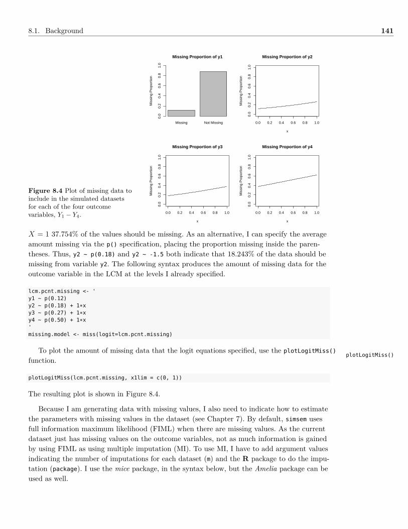
8.1. Background 141
Figure 8.4 Plot of missing data toinclude in the simulated datasetsfor each of the four outcomevariables, Y1 − Y4.
Missing Not Missing
Missing Proportion of y1
Mis
sing
Pro
port
ion
0.0
0.2
0.4
0.6
0.8
1.0
0.0 0.2 0.4 0.6 0.8 1.0
0.0
0.2
0.4
0.6
0.8
1.0
Missing Proportion of y2
x
Mis
sing
Pro
port
ion
0.0 0.2 0.4 0.6 0.8 1.0
0.0
0.2
0.4
0.6
0.8
1.0
Missing Proportion of y3
x
Mis
sing
Pro
port
ion
0.0 0.2 0.4 0.6 0.8 1.0
0.0
0.2
0.4
0.6
0.8
1.0
Missing Proportion of y4
x
Mis
sing
Pro
port
ion
X = 1 37.754% of the values should be missing. As an alternative, I can specify the averageamount missing via the p() specification, placing the proportion missing inside the paren-theses. Thus, y2 ~ p(0.18) and y2 ~ -1.5 both indicate that 18.243% of the data should bemissing from variable y2. The following syntax produces the amount of missing data for theoutcome variable in the LCM at the levels I already specified.
lcm.pcnt.missing <- 'y1 ~ p(0.12)y2 ~ p(0.18) + 1*xy3 ~ p(0.27) + 1*xy4 ~ p(0.50) + 1*x'missing.model <- miss(logit=lcm.pcnt.missing)
To plot the amount of missing data that the logit equations specified, use the plotLogitMiss()
function.
plotLogitMiss(lcm.pcnt.missing, x1lim = c(0, 1))
The resulting plot is shown in Figure 8.4.
Because I am generating data with missing values, I also need to indicate how to estimatethe parameters with missing values in the dataset (see Chapter 7). By default, simsem usesfull information maximum likelihood (FIML) when there are missing values. As the currentdataset just has missing values on the outcome variables, not as much information is gainedby using FIML as using multiple imputation (MI). To use MI, I have to add argument valuesindicating the number of imputations for each dataset (m) and the R package to do the impu-tation (package). I use the mice package, in the syntax below, but the Amelia package can beused as well.
plotLogitMiss()
142 Chapter 8. Sample Size Planning
missing.model <- miss(logit = lcm.pcnt.missing, m = 10, package = "mice")
I start the sample size study by specifying sample sizes from n = 200 to n = 300, in-creasing by 10. As I have to simulate multiple datasets for each sample size and I have toimpute the data for each simulated dataset, I set the number of imputed datasets to m = 10and only did p = 100 simulations per sample size. This still took a little over 30 minutes tocomplete.
lcm.missing.n <- sim(nRep=NULL, model=lcm.model, n=rep(seq(200,300,10), 100),generate=lcm.pop.model, lavaanfun = "growth", multicore=TRUE, miss=missing.model)
# get power estimates for each sample sizelcm.missing.pwr.n <- getPower(lcm.missing.n)
# Find the sample size needed for power = .0.8findPower(lcm.missing.pwr.n, "N", 0.8)
## i~x a y1~~y1 y2~~y2 y3~~y3 y4~~y4 i~~i s~~s i~~s i~1 s~1## 200 273 Inf Inf Inf 200 226 233 NA NA 200
The results indicate that approximately 273 respondents provide sufficient power for aregression coefficient of 0.20. I then did another MC study with p = 10, 000 repetitions forn = 273. I did the study two times, using two different seeds. Each study took over 3.50hours. I only show the results from one study to save space, but the power, bias, and cover-age from both studies were all at acceptable values.
lcm1.missing <- sim(nRep=10000, model=lcm.model, n =273, generate=lcm.pop.model,lavaanfun = "growth", multicore=TRUE, miss=missing.model, seed=4335)lcm2.missing <- sim(nRep=1000, model=lcm.model, n =273, generate=lcm.pop.model,lavaanfun = "growth", multicore=TRUE, miss=missing.model, seed=5443)summaryParam(lcm1.missing,alpha = 0.05,detail=TRUE)summaryParam(lcm2.missing,alpha = 0.05,detail=TRUE)
## Estimate.Average Estimate.SD Average.SE Power..Not.equal.0. Std.Est Std.Est.SD## a 0.193 0.069 0.068 0.805 0.32 0.121## Average.Param Average.Bias Coverage Rel.Bias Std.Bias Rel.SE.Bias Average.CI.Width## a 0.2 -0.007 0.939 -0.034 -0.098 -0.019 0.265## SD.CI.Width Average.FMI1 SD.FMI1 Average.FMI2 SD.FMI2## a 0.032 0.381 0.119 0.4 0.126
8.2 SummaryIn this chapter, I discussed sample size planning using a Monte Carlo (MC) simulation study.The MC method is very general and will work for any study that can be specified as a struc-tural equation model. I demonstrated how the sample size estimates from a MC study equalthe results from more traditional sample size methods when the model is very simple (e.g.,mean differences between two groups). I then showed how MC methods can encompass awider range of models than traditional methods, as well as incorporate missing data. I con-cluded the chapter by explicitly working through an example same size study for a longitudi-nal design that used a latent curve model.
8.3 Writing the ResultsTypically, sample size planning is just one component of a larger project, done before anydata is collected. Consequently, more is written about them in technical reports and grant
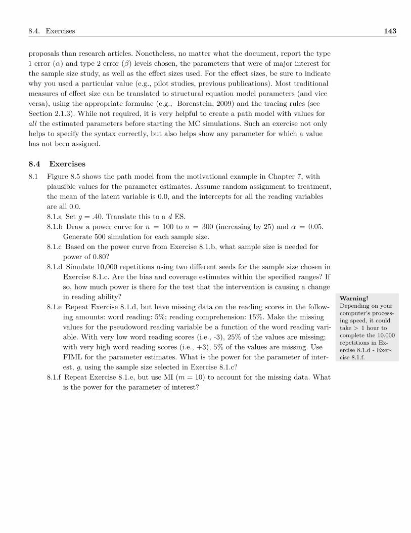
8.4. Exercises 143
proposals than research articles. Nonetheless, no matter what the document, report the type1 error (α) and type 2 error (β) levels chosen, the parameters that were of major interest forthe sample size study, as well as the effect sizes used. For the effect sizes, be sure to indicatewhy you used a particular value (e.g., pilot studies, previous publications). Most traditionalmeasures of effect size can be translated to structural equation model parameters (and viceversa), using the appropriate formulae (e.g., Borenstein, 2009) and the tracing rules (seeSection 2.1.3). While not required, it is very helpful to create a path model with values forall the estimated parameters before starting the MC simulations. Such an exercise not onlyhelps to specify the syntax correctly, but also helps show any parameter for which a valuehas not been assigned.
8.4 Exercises8.1 Figure 8.5 shows the path model from the motivational example in Chapter 7, with
plausible values for the parameter estimates. Assume random assignment to treatment,the mean of the latent variable is 0.0, and the intercepts for all the reading variablesare all 0.0.8.1.a Set g = .40. Translate this to a d ES.8.1.b Draw a power curve for n = 100 to n = 300 (increasing by 25) and α = 0.05.
Generate 500 simulation for each sample size.8.1.c Based on the power curve from Exercise 8.1.b, what sample size is needed for
power of 0.80?8.1.d Simulate 10,000 repetitions using two different seeds for the sample size chosen in
Exercise 8.1.c. Are the bias and coverage estimates within the specified ranges? Ifso, how much power is there for the test that the intervention is causing a changein reading ability?
8.1.e Repeat Exercise 8.1.d, but have missing data on the reading scores in the follow-ing amounts: word reading: 5%; reading comprehension: 15%. Make the missingvalues for the pseudoword reading variable be a function of the word reading vari-able. With very low word reading scores (i.e., -3), 25% of the values are missing;with very high word reading scores (i.e., +3), 5% of the values are missing. UseFIML for the parameter estimates. What is the power for the parameter of inter-est, g, using the sample size selected in Exercise 8.1.c?
8.1.f Repeat Exercise 8.1.e, but use MI (m = 10) to account for the missing data. Whatis the power for the parameter of interest?
Warning!Depending on yourcomputer’s process-ing speed, it couldtake > 1 hour tocomplete the 10,000repetitions in Ex-ercise 8.1.d - Exer-cise 8.1.f.
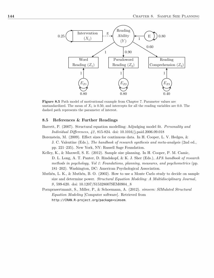
144 Chapter 8. Sample Size Planning
ReadingAbility(Y )
PseudowordReading (Z2)
WordReading (Z1)
ReadingComprehension (Z3)
EIntervention
(X1)
1 0.900.60
1g
EZ1 EZ2 EZ3
1 1 1
0.80 0.80 0.40
0.800.25
Figure 8.5 Path model of motivational example from Chapter 7. Parameter values areunstandardized. The mean of X1 is 0.50, and intercepts for all the reading variables are 0.0. Thedashed path represents the parameter of interest.
8.5 References & Further ReadingsBarrett, P. (2007). Structural equation modelling: Adjudging model fit. Personality and
Individual Differences, 42 , 815-824. doi: 10.1016/j.paid.2006.09.018Borenstein, M. (2009). Effect sizes for continuous data. In H. Cooper, L. V. Hedges, &
J. C. Valentine (Eds.), The handbook of research synthesis and meta-analysis (2nd ed.,pp. 221–235). New York, NY: Russell Sage Foundation.
Kelley, K., & Maxwell, S. E. (2012). Sample size planning. In H. Cooper, P. M. Camic,D. L. Long, A. T. Panter, D. Rindskopf, & K. J. Sher (Eds.), APA handbook of researchmethods in psychology, Vol 1: Foundations, planning, measures, and psychometrics (pp.181–202). Washington, DC: American Psychological Association.
Muthén, L. K., & Muthén, B. O. (2002). How to use a Monte Carlo study to decide on samplesize and determine power. Structural Equation Modeling: A Multidisciplinary Journal,9 , 599-620. doi: 10.1207/S15328007SEM0904_8
Pornprasertmanit, S., Miller, P., & Schoemann, A. (2012). simsem: SIMulated StructuralEquation Modeling [Computer software]. Retrieved fromhttp://CRAN.R-project.org/package=simsem.
9 | Hierarchical Latent VariableModels
Chapter Contents9.1 Background . . . . . . . . . . . . . . . . . . . . . . . . . . . . . . . . . . . . 145
9.1.1 Example: Hierarchical Latent Variable Models . . . . . . . . . . . . . 1489.2 Summary . . . . . . . . . . . . . . . . . . . . . . . . . . . . . . . . . . . . . . 1519.3 Writing the Results . . . . . . . . . . . . . . . . . . . . . . . . . . . . . . . . 1519.4 Exercises . . . . . . . . . . . . . . . . . . . . . . . . . . . . . . . . . . . . . . 1519.5 References & Further Readings . . . . . . . . . . . . . . . . . . . . . . . . . . 152
9.1 BackgroundThis chapter covers LVMs with hierarchical structures. The terminology used in the literatureon hierarchical LVMs can be confusing, not because the concepts are especially difficult, butbecause of the inconsistent use of terms. I have chosen to use the terms higher-order and bi-factor purposefully, as there is more consistency with their use than other terms. I used thehierarchical term to name this chapter because it has been used to describe both higher-orderand bi-factor models.
All the LVMs I have considered in this book have only included LVs that directly influ-ence the indicator variables. An extension of this model is a higher-order LVM. A higher-order model specifies that there are LVs that directly influence the indicator variables (calledfirst-order LVs [FOLV]) as well as LVs that directly influence the first-order LVs (i.e., second-order LVs [SOLV]).
Higher-order models are usually applicable when (a) there are multiple (≥ 3) FOLVsthat substantially covary with each other, and (b) there is a SOLV that is hypothesized toaccount for the relationship among the FOLVs. A typical higher-order model for cognitiveabilities data is one that posits that the SOLV general intelligence (g) is the sole reason whyvarious measures of cognitive ability, each of which are FOLVs, are related to each other (seeFigure 9.1a).
With higher-order models, the covariance of the FOLVs is accounted for by a SOLV thatrepresents a higher-order construct (i.e., what is in common among all the FOLV). Conse-quently, higher-order models decompose a FOLV into two separate parts: the part that isexplained by the SOLV and the part that is independent of the SOLV. This second part issometimes called a specific factor, but it is really just error, i.e., the portion of a FOLV’svariance that is unexplained by the SOLV. The FOLVs’ specific factors are typically uncorre-lated with the SOLV and among themselves.
Higher-OrderLatent Variable
Model
First-OrderLatent Variable
(FOLV)
Second-OrderLatent Variable
(SOLV)
There can be multi-ple SOLVs.
Specific Factor
145
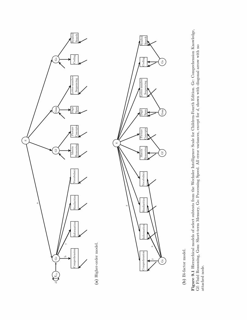
g
Matrix
Reasoning
Vocabu
lary
Simila
rities
Inform
ation
Com
prehensio
nPicture
Con
cepts
Digit
Span
Letter-num
ber
Sequ
encing
Cod
ing
Symbo
lSearch
Gf
Gsm
Gc
Gs
bc
a
E Gc
d (a)Highe
r-ordermod
el.
g
Matrix
Reasoning
Vocabu
lary
Simila
rities
Inform
ation
Com
prehensio
nPicture
Con
cepts
Digit
Span
Letter-num
ber
Sequ
encing
Cod
ing
Symbo
lSearch
Gf
Gsm
Gc
Gs
yx
z
(b)Bi-factormod
el.
Figure9.1Hierarchicalm
odelsof
select
subtests
from
theWechslerIntelligenc
eSc
aleforChildren-Fo
urth
Edition
.Gc:
Com
prehensio
nKno
wledg
e,Gf:FluidReasoning
,Gsm
:Sho
rt-term
Mem
ory,
Gs:
Processin
gSp
eed.
Allerrorvaria
nces,e
xcep
tford,
show
nwith
diag
onal
arrow
with
noattached
node
.
9.1. Background 147
With higher-order models, the influence of the SOLV on the manifest variables (MVs)is mediated by the FOLVs. That is, the SOLVs have an indirect influence on the MVs (seeSection 2.4). The value of a SOLV’s indirect influence on a MV can be estimated using thetracing rules (see Section 2.1.3). Specifically, the indirect influence is calculated by multiply-ing the loading on the FOLV by the FOLV’s loading on the SOLV’s (e.g., b× a in Figure 9.1a).Similarly, influence of a specific factor on a MV can be computed by multiplying the loadingon the FOLV by the standard deviation of the FOLV’s specific factor (e.g., b ×
√d in Fig-
ure 9.1a). The ratio of the SOLV’s indirect influence to the influence of the specific factor isthe exact same for all the indicator variables for a given FOLV. For example, in Figure 9.1a:
b× ab×√d
= c× ac×√d
Identification of a SOLV is similar to that with FOLVs (see Section 3.2.1). The differenceis that the unique information is not coming from the manifest variables, but the FOLVs.Thus, three FOLVs produce 3× 4/2 = 6 non-redundant pieces of information to estimate threespecific factors (error variances) and three loadings (or two loadings and one latent variance).Although the entire LVM may be overidentified, the SOLV part of the model is just-identifiedwith only three FOLVs. With four FOLVs, there are 4 × 5/2 = 10 non-redundant pieces ofinformation to estimate four specific factors and four loadings, making the SOLV part of themodel overidentified.
An alternative (actually, a generalization) to the higher-order model is a bi-factor model.Anexample is shown in Figure 9.1b. A bi-factor model specifies that all the LVs are FOLVs, butsome LVs are general (i.e., influence all the manifest variables) and some are domain spe-cific (i.e., influence a portion of the manifest variables). Moreover, all the FOLVs are speci-fied to be unrelated with each other, indicating that not only are the domain-specific factorsindependent of each other, but they are independent of the general LV as well.
Bi-factor models are usually applicable when: (a) there is a general factor that is hypoth-esized to account for the covariance among the MVs; (b) there are multiple domain-specificLVs, each of which is thought to have an unique influence beyond a general LV; and (c) inter-est is in the domain-specific LVs as well as the general LV.
There are some parallels between the higher-order and bi-factor models. First, the inter-pretation of the bi-factor model’s general LV and the higher-order models’ SOLV are similar.Second, the specific factors in the higher-order model are similar to the domain-specific LVsin the bi-factor model. Third, in both the bi-factor and higher-order models the FOLVs areall uncorrelated with each other.
There are some major distinctions between the two models, as well. The distinctionsmainly stem from the fact that in bi-factor models, the domain-specific LVs are totally in-dependent of the general LV, whereas with the higher-order model the SOLV has a direct in-fluence on the FOLVs. This independence yields some results for the bi-factor model that areimpossible with the higher-order model. First, bi-factor models allow for a direct examination
Bi-Factor Model
Domain-SpecificLatent Variable
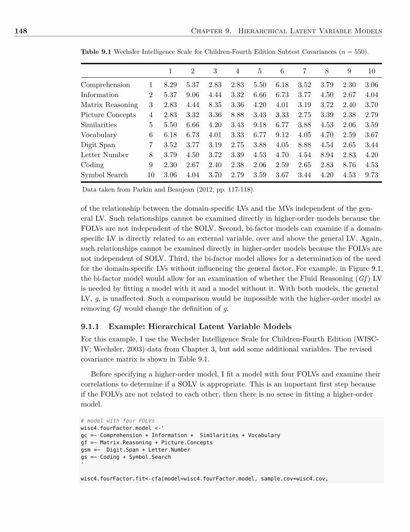
148 Chapter 9. Hierarchical Latent Variable Models
Table 9.1 Wechsler Intelligence Scale for Children-Fourth Edition Subtest Covariances (n = 550).
1 2 3 4 5 6 7 8 9 10
Comprehension 1 8.29 5.37 2.83 2.83 5.50 6.18 3.52 3.79 2.30 3.06Information 2 5.37 9.06 4.44 3.32 6.66 6.73 3.77 4.50 2.67 4.04Matrix Reasoning 3 2.83 4.44 8.35 3.36 4.20 4.01 3.19 3.72 2.40 3.70Picture Concepts 4 2.83 3.32 3.36 8.88 3.43 3.33 2.75 3.39 2.38 2.79Similarities 5 5.50 6.66 4.20 3.43 9.18 6.77 3.88 4.53 2.06 3.59Vocabulary 6 6.18 6.73 4.01 3.33 6.77 9.12 4.05 4.70 2.59 3.67Digit Span 7 3.52 3.77 3.19 2.75 3.88 4.05 8.88 4.54 2.65 3.44Letter Number 8 3.79 4.50 3.72 3.39 4.53 4.70 4.54 8.94 2.83 4.20Coding 9 2.30 2.67 2.40 2.38 2.06 2.59 2.65 2.83 8.76 4.53Symbol Search 10 3.06 4.04 3.70 2.79 3.59 3.67 3.44 4.20 4.53 9.73
Data taken from Parkin and Beaujean (2012, pp. 117-118).
of the relationship between the domain-specific LVs and the MVs independent of the gen-eral LV. Such relationships cannot be examined directly in higher-order models because theFOLVs are not independent of the SOLV. Second, bi-factor models can examine if a domain-specific LV is directly related to an external variable, over and above the general LV. Again,such relationships cannot be examined directly in higher-order models because the FOLVs arenot independent of SOLV. Third, the bi-factor model allows for a determination of the needfor the domain-specific LVs without influencing the general factor. For example, in Figure 9.1,the bi-factor model would allow for an examination of whether the Fluid Reasoning (Gf ) LVis needed by fitting a model with it and a model without it. With both models, the generalLV, g, is unaffected. Such a comparison would be impossible with the higher-order model asremoving Gf would change the definition of g.
9.1.1 Example: Hierarchical Latent Variable ModelsFor this example, I use the Wechsler Intelligence Scale for Children-Fourth Edition (WISC-IV; Wechsler, 2003) data from Chapter 3, but add some additional variables. The revisedcovariance matrix is shown in Table 9.1.
Before specifying a higher-order model, I fit a model with four FOLVs and examine theircorrelations to determine if a SOLV is appropriate. This is an important first step becauseif the FOLVs are not related to each other, then there is no sense in fitting a higher-ordermodel.
# model with four FOLVswisc4.fourFactor.model <-'gc =~ Comprehension + Information + Similarities + Vocabularygf =~ Matrix.Reasoning + Picture.Conceptsgsm =~ Digit.Span + Letter.Numbergs =~ Coding + Symbol.Search'
wisc4.fourFactor.fit<-cfa(model=wisc4.fourFactor.model, sample.cov=wisc4.cov,
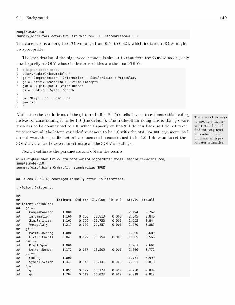
9.1. Background 149
sample.nobs=550)summary(wisc4.fourFactor.fit, fit.measure=TRUE, standardized=TRUE)
The correlations among the FOLVs range from 0.56 to 0.824, which indicate a SOLV mightbe appropriate.
The specification of the higher-order model is similar to that from the four-LV model, onlynow I specify a SOLV whose indicator variables are the four FOLVs.1 # higher-order model2 wisc4.higherOrder.model<-'3 gc =~ Comprehension + Information + Similarities + Vocabulary4 gf =~ Matrix.Reasoning + Picture.Concepts5 gsm =~ Digit.Span + Letter.Number6 gs =~ Coding + Symbol.Search78 g=~ NA*gf + gc + gsm + gs9 g~~ 1*g
10 '
Notice the the NA* in front of the gf term in line 8. This tells lavaan to estimate this loadinginstead of constraining it to be 1.0 (the default). The trade-off for doing this is that g’s vari-ance has to be constrained to 1.0, which I specify on line 9. I do this because I do not wantto constrain all the latent variables’ variances to be 1.0 with the std.lv=TRUE argument, as Ido not want the specific factors’ variances to be constrained to be 1.0. I do want to set theSOLV’s variance, however, to estimate all the SOLV’s loadings.
Next, I estimate the parameters and obtain the results.
wisc4.higherOrder.fit <- cfa(model=wisc4.higherOrder.model, sample.cov=wisc4.cov,sample.nobs=550)summary(wisc4.higherOrder.fit, standardized=TRUE)
## lavaan (0.5-16) converged normally after 55 iterations
..<Output Omitted>..
#### Estimate Std.err Z-value P(>|z|) Std.lv Std.all## Latent variables:## gc =~## Comprehension 1.000 2.194 0.762## Information 1.160 0.056 20.813 0.000 2.545 0.846## Similarities 1.165 0.056 20.753 0.000 2.555 0.844## Vocabulary 1.217 0.056 21.857 0.000 2.670 0.885## gf =~## Matrix.Resnng 1.000 1.990 0.689## Pictur.Cncpts 0.847 0.079 10.754 0.000 1.685 0.566## gsm =~## Digit.Span 1.000 1.967 0.661## Letter.Number 1.172 0.087 13.505 0.000 2.306 0.772## gs =~## Coding 1.000 1.771 0.599## Symbol.Search 1.441 0.142 10.141 0.000 2.551 0.818## g =~## gf 1.851 0.122 15.173 0.000 0.930 0.930## gc 1.794 0.112 16.023 0.000 0.818 0.818
There are other waysto specify a higher-order model, but Ifind this way tendsto produce fewerproblems with pa-rameter estimation.
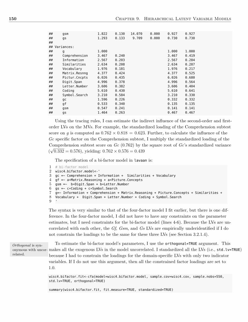
150 Chapter 9. Hierarchical Latent Variable Models
Orthogonal is syn-onymous with uncor-related.
## gsm 1.822 0.130 14.070 0.000 0.927 0.927## gs 1.293 0.133 9.709 0.000 0.730 0.730#### Variances:## g 1.000 1.000 1.000## Comprehension 3.467 0.240 3.467 0.419## Information 2.567 0.203 2.567 0.284## Similarities 2.634 0.208 2.634 0.287## Vocabulary 1.976 0.181 1.976 0.217## Matrix.Resnng 4.377 0.424 4.377 0.525## Pictur.Cncpts 6.026 0.435 6.026 0.680## Digit.Span 4.996 0.378 4.996 0.564## Letter.Number 3.606 0.382 3.606 0.404## Coding 5.610 0.430 5.610 0.641## Symbol.Search 3.210 0.584 3.210 0.330## gc 1.596 0.226 0.332 0.332## gf 0.533 0.340 0.135 0.135## gsm 0.547 0.241 0.141 0.141## gs 1.464 0.263 0.467 0.467
Using the tracing rules, I can estimate the indirect influence of the second-order and first-order LVs on the MVs. For example, the standardized loading of the Comprehension subtestscore on g is computed as 0.762 × 0.818 = 0.623. Further, to calculate the influence of theGc specific factor on the Comprehension subtest, I multiply the standardized loading of theComprehension subtest score on Gc (0.762) by the square root of Gc’s standardized variance(√
0.332 = 0.576), yielding: 0.762× 0.576 = 0.439
The specification of a bi-factor model in lavaan is:1 # bi-factor model2 wisc4.bifactor.model<-'3 gc =~ Comprehension + Information + Similarities + Vocabulary4 gf =~ a*Matrix.Reasoning + a*Picture.Concepts5 gsm =~ b*Digit.Span + b*Letter.Number6 gs =~ c*Coding + c*Symbol.Search7 g=~ Information + Comprehension + Matrix.Reasoning + Picture.Concepts + Similarities +8 Vocabulary + Digit.Span + Letter.Number + Coding + Symbol.Search9 '
The syntax is very similar to that of the four-factor model I fit earlier, but there is one dif-ference. In the four-factor model, I did not have to have any constraints on the parameterestimates, but I need constraints for the bi-factor model (lines 4-6). Because the LVs are un-correlated with each other, the Gf, Gsm, and Gs LVs are empirically underidentified if I donot constrain the loadings to be the same for these three LVs (see Section 3.2.1.4).
To estimate the bi-factor model’s parameters, I use the orthogonal=TRUE argument. Thismakes all the exogenous LVs in the model uncorrelated. I standardized all the LVs (i.e., std.lv=TRUE)because I had to constrain the loadings for the domain-specific LVs with only two indicatorvariables. If I do not use this argument, then all the constrained factor loadings are set to1.0.
wisc4.bifactor.fit<-cfa(model=wisc4.bifactor.model, sample.cov=wisc4.cov, sample.nobs=550,std.lv=TRUE, orthogonal=TRUE)
summary(wisc4.bifactor.fit, fit.measure=TRUE, standardized=TRUE)
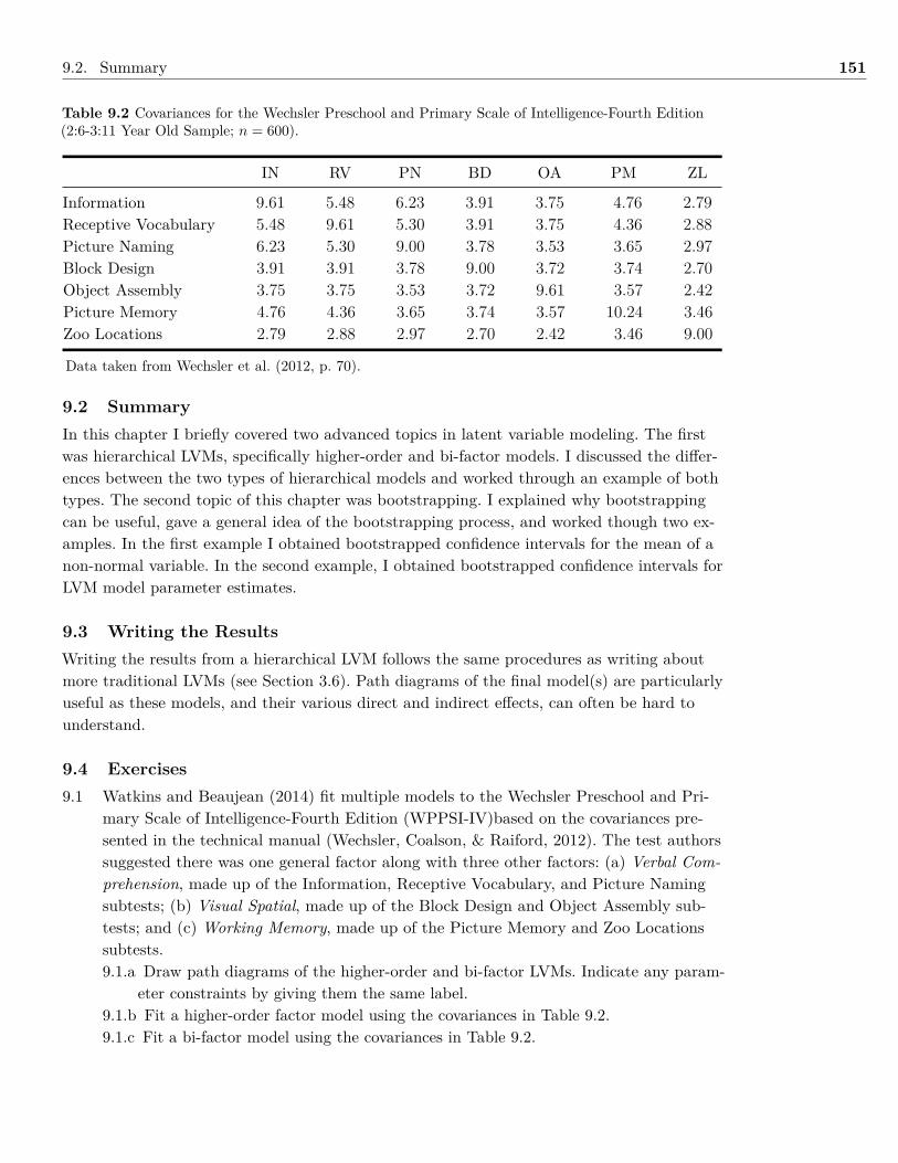
9.2. Summary 151
Table 9.2 Covariances for the Wechsler Preschool and Primary Scale of Intelligence-Fourth Edition(2:6-3:11 Year Old Sample; n = 600).
IN RV PN BD OA PM ZL
Information 9.61 5.48 6.23 3.91 3.75 4.76 2.79Receptive Vocabulary 5.48 9.61 5.30 3.91 3.75 4.36 2.88Picture Naming 6.23 5.30 9.00 3.78 3.53 3.65 2.97Block Design 3.91 3.91 3.78 9.00 3.72 3.74 2.70Object Assembly 3.75 3.75 3.53 3.72 9.61 3.57 2.42Picture Memory 4.76 4.36 3.65 3.74 3.57 10.24 3.46Zoo Locations 2.79 2.88 2.97 2.70 2.42 3.46 9.00
Data taken from Wechsler et al. (2012, p. 70).
9.2 SummaryIn this chapter I briefly covered two advanced topics in latent variable modeling. The firstwas hierarchical LVMs, specifically higher-order and bi-factor models. I discussed the differ-ences between the two types of hierarchical models and worked through an example of bothtypes. The second topic of this chapter was bootstrapping. I explained why bootstrappingcan be useful, gave a general idea of the bootstrapping process, and worked though two ex-amples. In the first example I obtained bootstrapped confidence intervals for the mean of anon-normal variable. In the second example, I obtained bootstrapped confidence intervals forLVM model parameter estimates.
9.3 Writing the ResultsWriting the results from a hierarchical LVM follows the same procedures as writing aboutmore traditional LVMs (see Section 3.6). Path diagrams of the final model(s) are particularlyuseful as these models, and their various direct and indirect effects, can often be hard tounderstand.
9.4 Exercises9.1 Watkins and Beaujean (2014) fit multiple models to the Wechsler Preschool and Pri-
mary Scale of Intelligence-Fourth Edition (WPPSI-IV)based on the covariances pre-sented in the technical manual (Wechsler, Coalson, & Raiford, 2012). The test authorssuggested there was one general factor along with three other factors: (a) Verbal Com-prehension, made up of the Information, Receptive Vocabulary, and Picture Namingsubtests; (b) Visual Spatial, made up of the Block Design and Object Assembly sub-tests; and (c) Working Memory, made up of the Picture Memory and Zoo Locationssubtests.9.1.a Draw path diagrams of the higher-order and bi-factor LVMs. Indicate any param-
eter constraints by giving them the same label.9.1.b Fit a higher-order factor model using the covariances in Table 9.2.9.1.c Fit a bi-factor model using the covariances in Table 9.2.
152 Chapter 9. Hierarchical Latent Variable Models
9.5 References & Further ReadingsBrunner, M., Nagy, G., & Wilhelm, O. (2012). A tutorial on hierarchically structured
constructs. Journal of Personality, 80 , 796-846. doi: 10.1111/j.1467-6494.2011.00749.xChen, F. F., West, S. G., & Sousa, K. H. (2006). A comparison of bifactor and second-order
models of quality of life. Multivariate Behavioral Research, 41 , 189-225. doi:10.1207/s15327906mbr4102_5
Parkin, J., & Beaujean, A. A. (2012). The effects of Wechsler Intelligence Scale forChildren-Fourth Edition cognitive abilities on math achievement. Journal of SchoolPsychology, 50 , 113-128. doi: 10.1016/j.jsp.2011.08.003
Schmiedek, F., & Li, S.-C. (2004). Toward an alternative representation for disentanglingage-associated differences in general and specific cognitive abilities. Psychology andAging, 19 , 40-56. doi: 10.1037/0882-7974.19.1.40
Watkins, M. W., & Beaujean, A. A. (2014). Bifactor structure of the Wechsler Preschool andPrimary Scale of Intelligence-Fourth Edition. School Psychology Quarterly, 29 , 53-63.doi: 10.1037/spq0000038
Wechsler, D. (2003). Wechsler intelligence scale for children (4th ed.). San Antonio, TX: ThePsychological Corporation.
Wechsler, D., Coalson, D. L., & Raiford, S. E. (2012). Wechsler preschool and primary scale ofintelligence technical and interpretive manual (4th ed.). San Antonio, TX: ThePsychological Corporation.
Yung, Y.-F., Thissen, D., & McLeod, L. D. (1999). On the relationship between thehigher-order factor model and the hierarchical factor model. Psychometrika, 64 ,113-128. doi: 10.1007/bf02294531
A | Measures of Model Fit
There is no area as contentious in the field of latent variable modeling as determining howwell a model fits the data. New research is published in this area very frequently, so it wouldbe relatively futile for me to indicate the best measures to use for assessing model fit. Instead,I present a variety of model fit measures and their general interpretation. To aid in the un-derstanding of the fit measures, I use the model from Section 3.2 throughout this appendix.I reproduce the path model in Figure A.1. Although I leave it up to the reader to determinehow to best use the measures, I provide one caution: just because a model fits the data wellby some fit index, it does not mean that it is the best model or even a valid model. Theory,not fit measures, needs to drive the use and interpretation of LVMs.
A.1 BackgroundFor a LVM, model fit refers to the ability of a model to reproduce the original covariancematrix. Most fit indexes only work with over identified models, but some (e.g., the residual-based ones) can work with just-identified models, as well.
The fit measures that lavaan computes by default are given in Table A.1. There are twoways to obtain fit measures in lavaan. The first is to use the fitMeasures() function. Themain arguments are the fitted model and fit measures to produce. For the latter, use thefit.measures argument with the names of the fit measures given as a character vector. Thesecond way to obtain fit measures is to use the summary() function with the fit.measures=TRUE
argument.1
There are multiple ways to categorize fit indexes. I start with the χ2 test and then presentsome alternative fit indexes (AFI) by family (i.e., ones that are based on similar criteria).
A.1.1 χ2 Test and Its VariantsLatent variable models are fit to data using fitting/discrepancy functions, which examinehow close the model-implied covariances (i.e., those calculated based on the model parame-ter estimates), C, are to the actual covariances calculated from the sample, S. The goal ofthe fit function is to have C and S be as close as possible, so the value returned from the fitfunction, f , is as small as possible.
There are a variety of fit functions, but the most common are those based on maximumlikelihood (ML) for continuous variables, and least squares (usually weighted) for categoricalvariables. I discuss those based on the ML estimator, but there are analogs to these statisticsfor (weighted) least squares estimators.
When I present thefit measures’ for-mulae, it is the MLversion for a singlegroup. With multi-ple groups or least-squares estimationthe measures aresimilar, but not al-ways the same.
fitMeasures()
1 Another method that is “unfinished” is lavaan:::print.fit.measures(fitMeasures()), which returns theall the fit measures with their full names.
153
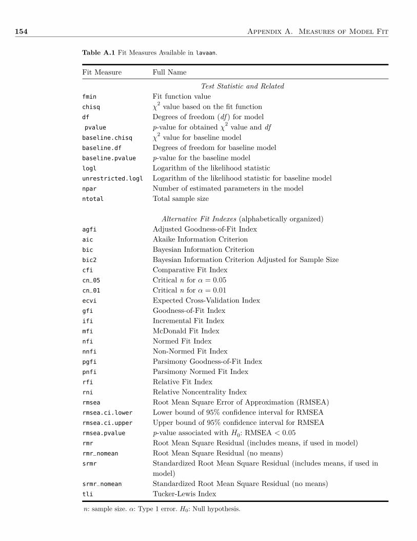
154 Appendix A. Measures of Model Fit
Table A.1 Fit Measures Available in lavaan.
Fit Measure Full Name
Test Statistic and Relatedfmin Fit function valuechisq χ
2 value based on the fit functiondf Degrees of freedom (df ) for modelpvalue p-value for obtained χ2 value and dfbaseline.chisq χ
2 value for baseline modelbaseline.df Degrees of freedom for baseline modelbaseline.pvalue p-value for the baseline modellogl Logarithm of the likelihood statisticunrestricted.logl Logarithm of the likelihood statistic for baseline modelnpar Number of estimated parameters in the modelntotal Total sample size
Alternative Fit Indexes (alphabetically organized)agfi Adjusted Goodness-of-Fit Indexaic Akaike Information Criterionbic Bayesian Information Criterionbic2 Bayesian Information Criterion Adjusted for Sample Sizecfi Comparative Fit Indexcn_05 Critical n for α = 0.05cn_01 Critical n for α = 0.01ecvi Expected Cross-Validation Indexgfi Goodness-of-Fit Indexifi Incremental Fit Indexmfi McDonald Fit Indexnfi Normed Fit Indexnnfi Non-Normed Fit Indexpgfi Parsimony Goodness-of-Fit Indexpnfi Parsimony Normed Fit Indexrfi Relative Fit Indexrni Relative Noncentrality Indexrmsea Root Mean Square Error of Approximation (RMSEA)rmsea.ci.lower Lower bound of 95% confidence interval for RMSEArmsea.ci.upper Upper bound of 95% confidence interval for RMSEArmsea.pvalue p-value associated with H0: RMSEA < 0.05rmr Root Mean Square Residual (includes means, if used in model)rmr_nomean Root Mean Square Residual (no means)srmr Standardized Root Mean Square Residual (includes means, if used in
model)srmr_nomean Standardized Root Mean Square Residual (no means)tli Tucker-Lewis Index
n: sample size. α: Type 1 error. H0: Null hypothesis.
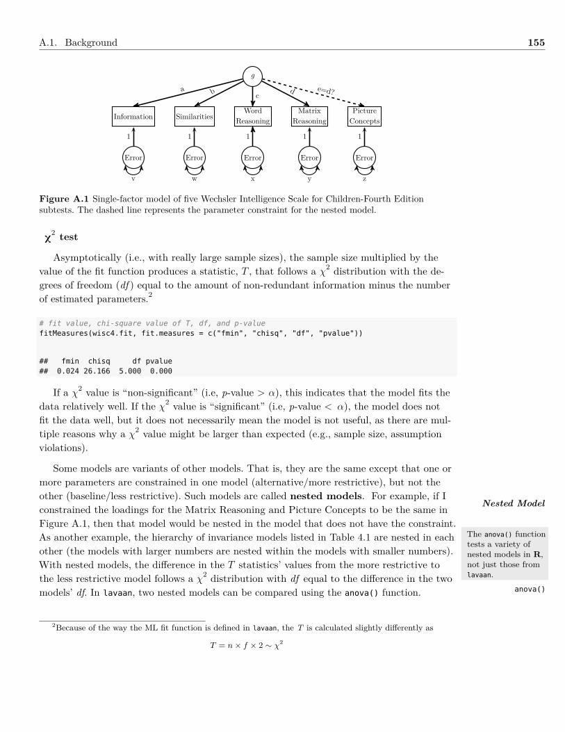
A.1. Background 155
g
WordReasoningSimilaritiesInformation
MatrixReasoning
PictureConcepts
Error Error Error Error Error
a b cd e=d?
1 1 1 1 1
v w x y z
Figure A.1 Single-factor model of five Wechsler Intelligence Scale for Children-Fourth Editionsubtests. The dashed line represents the parameter constraint for the nested model.
χ2 test
Asymptotically (i.e., with really large sample sizes), the sample size multiplied by thevalue of the fit function produces a statistic, T , that follows a χ2 distribution with the de-grees of freedom (df ) equal to the amount of non-redundant information minus the numberof estimated parameters.2
# fit value, chi-square value of T, df, and p-valuefitMeasures(wisc4.fit, fit.measures = c("fmin", "chisq", "df", "pvalue"))
## fmin chisq df pvalue## 0.024 26.166 5.000 0.000
If a χ2 value is “non-significant” (i.e, p-value > α), this indicates that the model fits thedata relatively well. If the χ2 value is “significant” (i.e, p-value < α), the model does notfit the data well, but it does not necessarily mean the model is not useful, as there are mul-tiple reasons why a χ2 value might be larger than expected (e.g., sample size, assumptionviolations).
Some models are variants of other models. That is, they are the same except that one ormore parameters are constrained in one model (alternative/more restrictive), but not theother (baseline/less restrictive). Such models are called nested models. For example, if Iconstrained the loadings for the Matrix Reasoning and Picture Concepts to be the same inFigure A.1, then that model would be nested in the model that does not have the constraint.As another example, the hierarchy of invariance models listed in Table 4.1 are nested in eachother (the models with larger numbers are nested within the models with smaller numbers).With nested models, the difference in the T statistics’ values from the more restrictive tothe less restrictive model follows a χ2 distribution with df equal to the difference in the twomodels’ df. In lavaan, two nested models can be compared using the anova() function.
Nested Model
The anova() functiontests a variety ofnested models in R,not just those fromlavaan.
anova()
2Because of the way the ML fit function is defined in lavaan, the T is calculated slightly differently as
T = n× f × 2 ∼ χ2
156 Appendix A. Measures of Model Fit
Robust Estimator
Most fit measuresin lavaan that werederived from a ro-bust estimatorhave a .scaled suf-fix in the name, e.g.,chisq.scaled.
anova(wisc4.fit, wisc4.2.fit)
## Chi Square Difference Test#### Df AIC BIC Chisq Chisq diff Df diff Pr(>Chisq)## wisc4.fit 5 12689 12732 26.2## wisc4.2.fit 6 12690 12729 29.4 3.21 1 0.073 .## ---## Signif. codes: 0 '***' 0.001 '**' 0.01 '*' 0.05 '.' 0.1 ' ' 1
A.1.1.1 Robust χ2 EstimatesThe χ2 test is valid only if the observations are independent, the non-standardized samplecovariance matrix is used, the sample size is sufficiently large, and the manifest endogenousvariables follow a multivariate normal distribution. The last assumption is usually the hard-est to meet. For situations when the data do not meet the normality requirement, one optionis to find a correction for the T statistic. These corrections involve using the mean or themean and variances to adjust the fit function. Estimators that employ any of these correc-tions are called robust estimators. The test statistics derived from the robust estimators(and their associated robust standard errors) are generally more accurate than the more tra-ditional test statistic when data are non-normal. Table A.2 gives a list of lavaan’s robustestimators.
Two of the most common ML corrections are the ones developed by Satorra and Bentler(1994) and by Yuan and Bentler (1998). For both estimators, correcting the T value for non-normality requires the estimation of a correction factor, c, which reflects the amount of aver-age multivariate kurtosis. To obtain the corrected T value, T ∗, multiply T by c. T ∗ follows aχ
2 distribution with df equal to the amount of non-redundant information minus the numberof estimated parameters.
Testing the difference between nested models using a robust estimator requires taking thecorrection factor into account. The correction factor for testing the difference between thebaseline (less restrictive, T1) and nested (more restrictive, T0) model, cd, is
cd = df0c0 − df1c1df0 − df1
wheredfi are the degrees of freedom for model i, andci is the correction factor for model i.
The corrected difference test statistic, T ∗d is
T ∗d = T0 − T1cd
whereTi is the uncorrected χ2 value for model i.
The anova() function will take the correction into account when comparing models.

TableA.2
Rob
ustEs
timatorsAv
ailablein
lavaan.
Estim
ator
Varia
ntDescriptio
n
Maxim
umLikelih
ood(M
L)MLM
Estim
ationwith
robu
ststan
dard
errors
andSa
torra-Bentle
rscaled
test
statist
ic.F
orcompleteda
taon
ly.
MLMVS
Estim
ationwith
robu
ststan
dard
errors
andamean-
andvaria
nce-ad
justed
test
statist
ic(Satterthw
aite
approa
ch).
Forcompleteda
taon
ly.
MLMV
Estim
ationwith
robu
ststan
dard
errors
andamean-
andvaria
nce-ad
justed
test
statist
ic(scale-shifted
approa
ch).
Forcompleteda
taon
ly.
MLF
Estim
ationwith
stan
dard
errors
basedon
thefirst-order
deriv
atives
andaconv
entio
nalt
eststatist
ic.F
orbo
thcompletean
dincompleteda
ta.
MLR
Estim
ationwith
robu
st(H
uber-W
hite)stan
dard
errors
andascaled
test
statist
icthat
isasym
ptotically
equa
lto
theYu
an-B
entle
rtest
statist
ic.F
orbo
thcompletean
dincompleteda
ta.
Least-Sq
uares(D
WLS
/ULS
)WLSM
a,b
Weigh
tedleastsqua
resestim
ationwith
robu
ststan
dard
errors
andamean-ad
justed
test
statist
ic.F
orcomplete
data
only.
WLSMVS
a,b
Weigh
tedleastsqua
resestim
ationwith
robu
ststan
dard
errors
andamean-
andvaria
nce-ad
justed
test
statist
ic(Satterthw
aite
approach).Fo
rcompleteda
taon
ly.
WLSMV
a,b
Weigh
tedleastsqua
resestim
ationwith
robu
ststan
dard
errors
andamean-
andvaria
nce-ad
justed
test
statist
ic(scale-shifted
approach).Fo
rcompleteda
taon
ly.
ULSM
Unw
eigh
tedleastsqua
resestim
ationwith
robu
ststan
dard
errors
andamean-ad
justed
test
statist
ic.F
orcomplete
data
only.
ULSMVS
Unw
eigh
tedleastsqua
resestim
ationwith
robu
ststan
dard
errors
andamean-
andvaria
nce-ad
justed
test
statist
ic(Satterthw
aite
approach).Fo
rcompleteda
taon
ly.
ULSMV
Unw
eigh
tedleastsqua
resestim
ationwith
robu
ststan
dard
errors
andamean-
andvaria
nce-ad
justed
test
statist
ic(scale-shifted
approach).Fo
rcompleteda
taon
ly.
aFo
rtherobu
stweigh
tedleastsqua
resvaria
nts(W
LSM,W
LSMVS,
WLS
MV),
lavaanuses
thediag
onal
oftheweigh
tmatrix
forestim
ation,
but
uses
thefullweigh
tmatrix
tocorrectthestan
dard
errors
andto
compu
tethetest
statist
ic.
bAsof
version05
.15in
lavaan,c
ategorical
data
canha
vemiss
ingda
tausingmissing="pairwise"argu
ment.
158 Appendix A. Measures of Model Fit
Alternative FitIndex
# robust ML estimators (MLM/Satorra-Bentler)wisc4.fit.mlm <- cfa(wisc4.model, data = wisc4.data, estimator = "MLM")wisc4.2.fit.mlm <- cfa(wisc4.2.model, data = wisc4.data, estimator = "MLM")# compare modelsanova(wisc4.fit.mlm, wisc4.2.fit.mlm)
## Scaled Chi Square Difference Test (test = satorra.bentler)#### Df AIC BIC Chisq Chisq diff Df diff Pr(>Chisq)## wisc4.fit.mlm 5 12699 12764 26## wisc4.2.fit.mlm 6 12700 12761 30 3.84 1 0.05 *## ---## Signif. codes: 0 '***' 0.001 '**' 0.01 '*' 0.05 '.' 0.1 ' ' 1
The T statistic (and its associated χ2 value) has a long history of use with LVMs, but hassome flaws, such as being strongly influenced by sample size–the larger the sample size, ce-teris paribus, the more likely the χ2 value will be statistically “significant”. Consequently avariety of alternative fit indexes (AFIs) have been developed to assess model fit. TheseAFIs are not test statistics, so they do not follow a particular probability distribution. In-stead, simulation studies and rules-of-thumb tend to dictate what values to use to indicatewhether a model fits the data.
A.2 Alternative Fit IndexesTo make their presentation easier to comprehend, I classify the alternative fit indexes (AFIs)into three different families.
1. Incremental indexes (sometimes called relative or comparative fit indexes).These indexes determine model fit through the comparison of the model of interestwith a baseline model. The baseline model (sometimes called the null or independencemodel) is a model where the only estimated parameters are the variances of the man-ifest variables (and the means or thresholds if they are part of the model). The df forthe null model are m(m− 1)/2, where m is the number of variables in the model.
2. Parsimony indexesThese indexes are constructed so that the model complexity is taken into account whenassessing model fit. In general, models with more parameters (fewer degrees of freedom)are penalized. Sometimes these indexes use the parsimony index, which is df
df0where df
is the model of interest’s degrees of freedom and df0 is the degrees of freedom for thebaseline model.
3. Absolute (Standalone) indexesThese indexes do not compare models or account for complexity. Hence, they measurethe absolute fit of the model.
A.2. Alternative Fit Indexes 159
A.2.1 Incremental IndexesComparative Fit Index (CFI)
CFI = 1− max[χ2I − dfI , 0]
max[χ2I − dfI , χ2
B − dfB, 0]where B subscripts the baseline model, I subscripts the model of interest, and max[ ] repre-sents the maximum of the values within the brackets.
CFI values closer to 1.0 indicate better fit.
fitMeasures(wisc4.fit, fit.measures = "cfi")
## cfi## 0.98
Normed Fit Index (NFI)/∆1
NFI = 1− fBfI
= 1− χ2B
χ2I
where f is the value of the fit function (or χ2 is the χ2 based on the fit function), B sub-scripts the baseline model, and I subscripts the model of interest.
NFI values closer to 1.0 indicate better fit.
fitMeasures(wisc4.fit, fit.measures = "nfi")
## nfi## 0.975
Parsimonious Normed Fit Index (PNFI)
PNFI = 1− dfI(fB − fI)dfB(fB)
where f is the value of the fit function, df are the degrees of freedom, B subscripts the base-line model, and I subscripts the model of interest.
The PNFI is a modification of the NFI that takes parsimony of the model into account.PNFI values closer to 1.0 indicate better fit.
fitMeasures(wisc4.fit, fit.measures = "pnfi")
## pnfi## 0.488
Incremental Fit Index (IFI)/∆2/Bollen’s Nonnormed Fit Index (NNFI)
IFI/NNFI = χ2B − χ
2I
χ2B − dfI
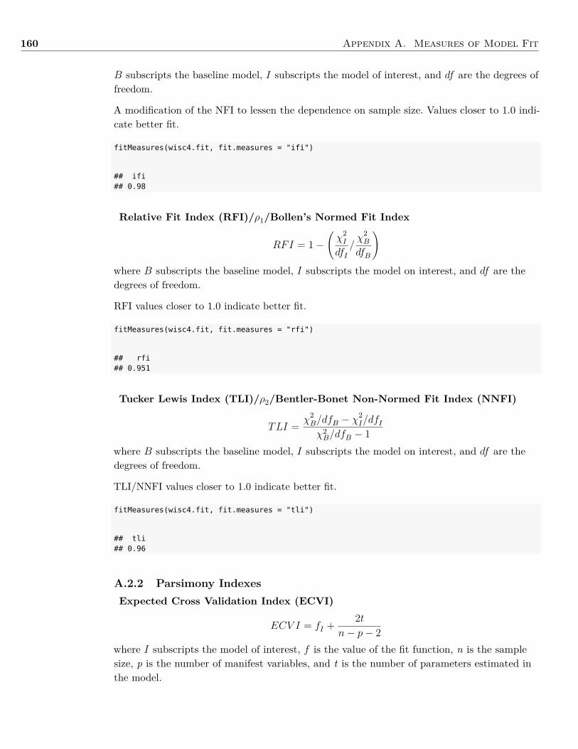
160 Appendix A. Measures of Model Fit
B subscripts the baseline model, I subscripts the model of interest, and df are the degrees offreedom.
A modification of the NFI to lessen the dependence on sample size. Values closer to 1.0 indi-cate better fit.
fitMeasures(wisc4.fit, fit.measures = "ifi")
## ifi## 0.98
Relative Fit Index (RFI)/ρ1/Bollen’s Normed Fit Index
RFI = 1−(χ
2I
dfI/χ
2B
dfB
)where B subscripts the baseline model, I subscripts the model on interest, and df are thedegrees of freedom.
RFI values closer to 1.0 indicate better fit.
fitMeasures(wisc4.fit, fit.measures = "rfi")
## rfi## 0.951
Tucker Lewis Index (TLI)/ρ2/Bentler-Bonet Non-Normed Fit Index (NNFI)
TLI = χ2B/dfB − χ
2I/dfI
χ2B/dfB − 1
where B subscripts the baseline model, I subscripts the model on interest, and df are thedegrees of freedom.
TLI/NNFI values closer to 1.0 indicate better fit.
fitMeasures(wisc4.fit, fit.measures = "tli")
## tli## 0.96
A.2.2 Parsimony IndexesExpected Cross Validation Index (ECVI)
ECV I = fI + 2tn− p− 2
where I subscripts the model of interest, f is the value of the fit function, n is the samplesize, p is the number of manifest variables, and t is the number of parameters estimated inthe model.
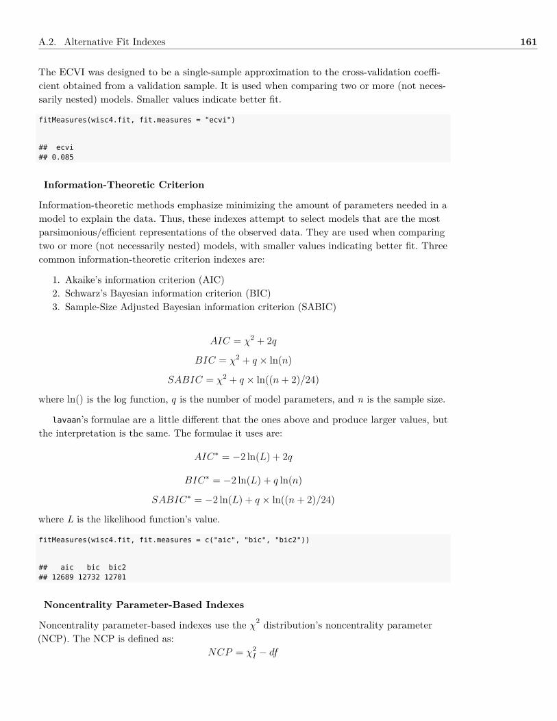
A.2. Alternative Fit Indexes 161
The ECVI was designed to be a single-sample approximation to the cross-validation coeffi-cient obtained from a validation sample. It is used when comparing two or more (not neces-sarily nested) models. Smaller values indicate better fit.
fitMeasures(wisc4.fit, fit.measures = "ecvi")
## ecvi## 0.085
Information-Theoretic Criterion
Information-theoretic methods emphasize minimizing the amount of parameters needed in amodel to explain the data. Thus, these indexes attempt to select models that are the mostparsimonious/efficient representations of the observed data. They are used when comparingtwo or more (not necessarily nested) models, with smaller values indicating better fit. Threecommon information-theoretic criterion indexes are:
1. Akaike’s information criterion (AIC)2. Schwarz’s Bayesian information criterion (BIC)3. Sample-Size Adjusted Bayesian information criterion (SABIC)
AIC = χ2 + 2q
BIC = χ2 + q × ln(n)
SABIC = χ2 + q × ln((n+ 2)/24)
where ln() is the log function, q is the number of model parameters, and n is the sample size.
lavaan’s formulae are a little different that the ones above and produce larger values, butthe interpretation is the same. The formulae it uses are:
AIC∗ = −2 ln(L) + 2q
BIC∗ = −2 ln(L) + q ln(n)
SABIC∗ = −2 ln(L) + q × ln((n+ 2)/24)
where L is the likelihood function’s value.
fitMeasures(wisc4.fit, fit.measures = c("aic", "bic", "bic2"))
## aic bic bic2## 12689 12732 12701
Noncentrality Parameter-Based Indexes
Noncentrality parameter-based indexes use the χ2 distribution’s noncentrality parameter(NCP). The NCP is defined as:
NCP = χ2I − df
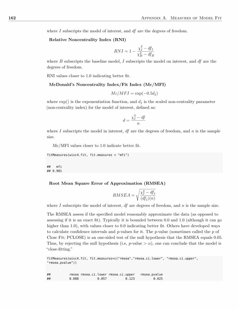
162 Appendix A. Measures of Model Fit
where I subscripts the model of interest, and df are the degrees of freedom.
Relative Noncentrality Index (RNI)
RNI = 1− χ2I − dfI
χ2B − dfB
where B subscripts the baseline model, I subscripts the model on interest, and df are thedegrees of freedom.
RNI values closer to 1.0 indicating better fit.
McDonald’s Noncentrality Index/Fit Index (Mc/MFI)
Mc/MFI = exp(−0.5dI)
where exp() is the exponentiation function, and dI is the scaled non-centrality parameter(non-centrality index) for the model of interest, defined as:
d = χ2I − dfn
where I subscripts the model in interest, df are the degrees of freedom, and n is the samplesize.
Mc/MFI values closer to 1.0 indicate better fit.
fitMeasures(wisc4.fit, fit.measures = "mfi")
## mfi## 0.981
Root Mean Square Error of Approximation (RMSEA)
RMSEA =√χ2I − dfI
(dfI)(n)where I subscripts the model of interest, df are degrees of freedom, and n is the sample size.
The RMSEA assess if the specified model reasonably approximate the data (as opposed toassessing if it is an exact fit). Typically it is bounded between 0.0 and 1.0 (although it can gohigher than 1.0), with values closer to 0.0 indicating better fit. Others have developed waysto calculate confidence intervals and p-values for it. The p-value (sometimes called the p ofClose Fit; PCLOSE) is an one-sided test of the null hypothesis that the RMSEA equals 0.05.Thus, by rejecting the null hypothesis (i.e, p-value > α), one can conclude that the model is“close-fitting.”
fitMeasures(wisc4.fit, fit.measures=c("rmsea","rmsea.ci.lower", "rmsea.ci.upper","rmsea.pvalue"))
## rmsea rmsea.ci.lower rmsea.ci.upper rmsea.pvalue## 0.088 0.057 0.123 0.025
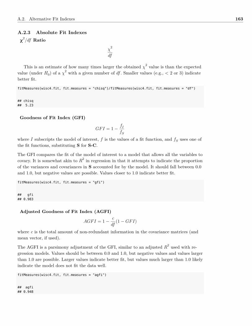
A.2. Alternative Fit Indexes 163
A.2.3 Absolute Fit Indexesχ
2/df Ratio
χ2
df
This is an estimate of how many times larger the obtained χ2 value is than the expectedvalue (under H0) of a χ
2 with a given number of df . Smaller values (e.g., < 2 or 3) indicatebetter fit.
fitMeasures(wisc4.fit, fit.measures = "chisq")/fitMeasures(wisc4.fit, fit.measures = "df")
## chisq## 5.23
Goodness of Fit Index (GFI)
GFI = 1− fIfS
where I subscripts the model of interest, f is the values of a fit function, and fS uses one ofthe fit functions, substituting S for S-C.
The GFI compares the fit of the model of interest to a model that allows all the variables tocovary. It is somewhat akin to R2 in regression in that it attempts to indicate the proportionof the variances and covariances in S accounted for by the model. It should fall between 0.0and 1.0, but negative values are possible. Values closer to 1.0 indicate better fit.
fitMeasures(wisc4.fit, fit.measures = "gfi")
## gfi## 0.983
Adjusted Goodness of Fit Index (AGFI)
AGFI = 1− c
df(1−GFI)
where c is the total amount of non-redundant information in the covariance matrices (andmean vector, if used).
The AGFI is a parsimony adjustment of the GFI, similar to an adjusted R2 used with re-gression models. Values should be between 0.0 and 1.0, but negative values and values largerthan 1.0 are possible. Larger values indicate better fit, but values much larger than 1.0 likelyindicate the model does not fit the data well.
fitMeasures(wisc4.fit, fit.measures = "agfi")
## agfi## 0.948
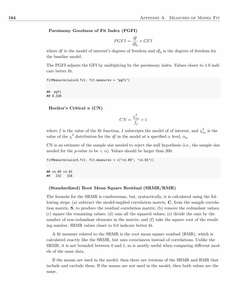
164 Appendix A. Measures of Model Fit
Parsimony Goodness of Fit Index (PGFI)
PGFI = df
df0×GFI
where df is the model of interest’s degrees of freedom and df0 is the degrees of freedom forthe baseline model.
The PGFI adjusts the GFI by multiplying by the parsimony index. Values closer to 1.0 indi-cate better fit.
fitMeasures(wisc4.fit, fit.measures = "pgfi")
## pgfi## 0.328
Hoelter’s Critical n (CN)
CN =χ
2α0
fI+ 1
where f is the value of the fit function, I subscripts the model of of interest, and χ2α0
is thevalue of the χ2 distribution for the df in the model at a specified α level, α0.
CN is an estimate of the sample size needed to reject the null hypothesis (i.e., the sample sizeneeded for the p-value to be < α). Values should be larger than 200.
fitMeasures(wisc4.fit, fit.measures = c("cn_05", "cn_01"))
## cn_05 cn_01## 232 316
(Standardized) Root Mean Square Residual (SRMR/RMR)
The formula for the SRMR is cumbersome, but, syntactically, it is calculated using the fol-lowing steps: (a) subtract the model-implied correlation matrix, C, from the sample correla-tion matrix, S, to produce the residual correlation matrix; (b) remove the redundant values;(c) square the remaining values; (d) sum all the squared values; (e) divide the sum by thenumber of non-redundant elements in the matrix; and (f) take the square root of the result-ing number. SRMR values closer to 0.0 indicate better fit.
A fit measure related to the SRMR is the root mean square residual (RMR), which iscalculated exactly like the SRMR, but uses covariances instead of correlations. Unlike theSRMR, it is not bounded between 0 and 1, so is mostly useful when comparing different mod-els of the same data.
If the means are used in the model, then there are versions of the SRMR and RMR thatinclude and exclude them. If the means are not used in the model, then both values are thesame.
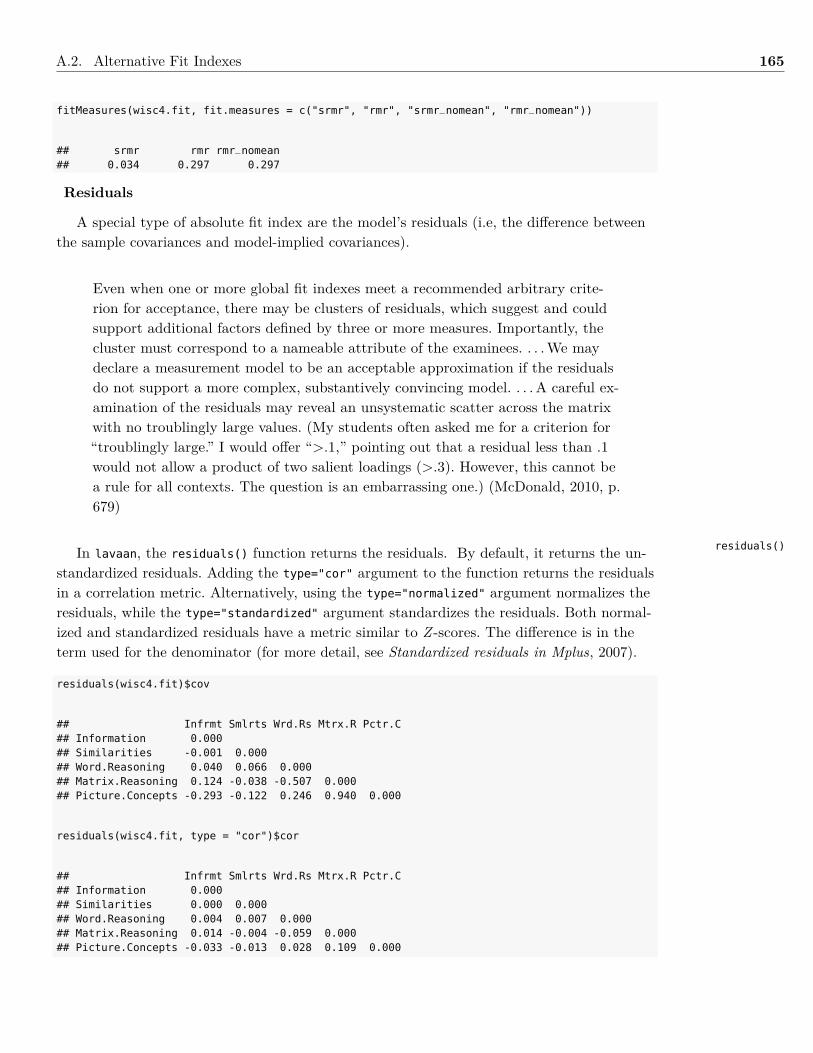
A.2. Alternative Fit Indexes 165
fitMeasures(wisc4.fit, fit.measures = c("srmr", "rmr", "srmr_nomean", "rmr_nomean"))
## srmr rmr rmr_nomean## 0.034 0.297 0.297
Residuals
A special type of absolute fit index are the model’s residuals (i.e, the difference betweenthe sample covariances and model-implied covariances).
Even when one or more global fit indexes meet a recommended arbitrary crite-rion for acceptance, there may be clusters of residuals, which suggest and couldsupport additional factors defined by three or more measures. Importantly, thecluster must correspond to a nameable attribute of the examinees. . . .We maydeclare a measurement model to be an acceptable approximation if the residualsdo not support a more complex, substantively convincing model. . . . A careful ex-amination of the residuals may reveal an unsystematic scatter across the matrixwith no troublingly large values. (My students often asked me for a criterion for“troublingly large.” I would offer “>.1,” pointing out that a residual less than .1would not allow a product of two salient loadings (>.3). However, this cannot bea rule for all contexts. The question is an embarrassing one.) (McDonald, 2010, p.679)
In lavaan, the residuals() function returns the residuals. By default, it returns the un-standardized residuals. Adding the type="cor" argument to the function returns the residualsin a correlation metric. Alternatively, using the type="normalized" argument normalizes theresiduals, while the type="standardized" argument standardizes the residuals. Both normal-ized and standardized residuals have a metric similar to Z -scores. The difference is in theterm used for the denominator (for more detail, see Standardized residuals in Mplus, 2007).
residuals(wisc4.fit)$cov
## Infrmt Smlrts Wrd.Rs Mtrx.R Pctr.C## Information 0.000## Similarities -0.001 0.000## Word.Reasoning 0.040 0.066 0.000## Matrix.Reasoning 0.124 -0.038 -0.507 0.000## Picture.Concepts -0.293 -0.122 0.246 0.940 0.000
residuals(wisc4.fit, type = "cor")$cor
## Infrmt Smlrts Wrd.Rs Mtrx.R Pctr.C## Information 0.000## Similarities 0.000 0.000## Word.Reasoning 0.004 0.007 0.000## Matrix.Reasoning 0.014 -0.004 -0.059 0.000## Picture.Concepts -0.033 -0.013 0.028 0.109 0.000
residuals()
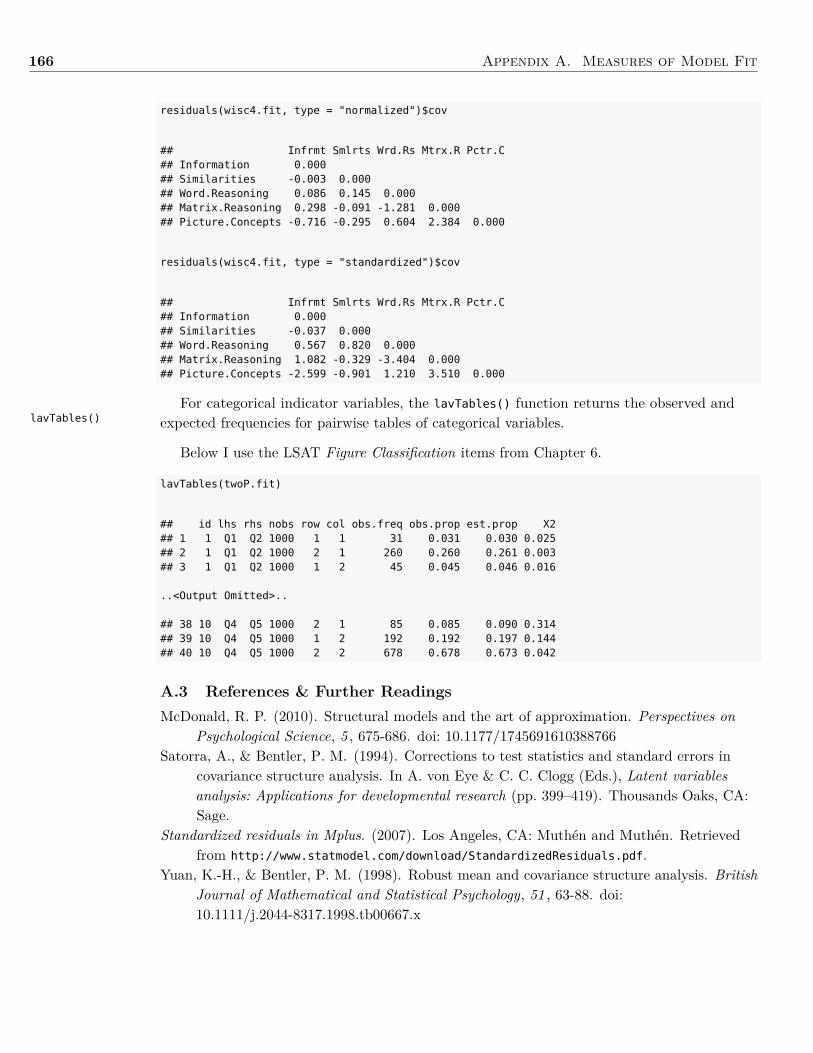
166 Appendix A. Measures of Model Fit
lavTables()
residuals(wisc4.fit, type = "normalized")$cov
## Infrmt Smlrts Wrd.Rs Mtrx.R Pctr.C## Information 0.000## Similarities -0.003 0.000## Word.Reasoning 0.086 0.145 0.000## Matrix.Reasoning 0.298 -0.091 -1.281 0.000## Picture.Concepts -0.716 -0.295 0.604 2.384 0.000
residuals(wisc4.fit, type = "standardized")$cov
## Infrmt Smlrts Wrd.Rs Mtrx.R Pctr.C## Information 0.000## Similarities -0.037 0.000## Word.Reasoning 0.567 0.820 0.000## Matrix.Reasoning 1.082 -0.329 -3.404 0.000## Picture.Concepts -2.599 -0.901 1.210 3.510 0.000
For categorical indicator variables, the lavTables() function returns the observed andexpected frequencies for pairwise tables of categorical variables.
Below I use the LSAT Figure Classification items from Chapter 6.
lavTables(twoP.fit)
## id lhs rhs nobs row col obs.freq obs.prop est.prop X2## 1 1 Q1 Q2 1000 1 1 31 0.031 0.030 0.025## 2 1 Q1 Q2 1000 2 1 260 0.260 0.261 0.003## 3 1 Q1 Q2 1000 1 2 45 0.045 0.046 0.016
..<Output Omitted>..
## 38 10 Q4 Q5 1000 2 1 85 0.085 0.090 0.314## 39 10 Q4 Q5 1000 1 2 192 0.192 0.197 0.144## 40 10 Q4 Q5 1000 2 2 678 0.678 0.673 0.042
A.3 References & Further ReadingsMcDonald, R. P. (2010). Structural models and the art of approximation. Perspectives on
Psychological Science, 5 , 675-686. doi: 10.1177/1745691610388766Satorra, A., & Bentler, P. M. (1994). Corrections to test statistics and standard errors in
covariance structure analysis. In A. von Eye & C. C. Clogg (Eds.), Latent variablesanalysis: Applications for developmental research (pp. 399–419). Thousands Oaks, CA:Sage.
Standardized residuals in Mplus. (2007). Los Angeles, CA: Muthén and Muthén. Retrievedfrom http://www.statmodel.com/download/StandardizedResiduals.pdf.
Yuan, K.-H., & Bentler, P. M. (1998). Robust mean and covariance structure analysis. BritishJournal of Mathematical and Statistical Psychology, 51 , 63-88. doi:10.1111/j.2044-8317.1998.tb00667.x
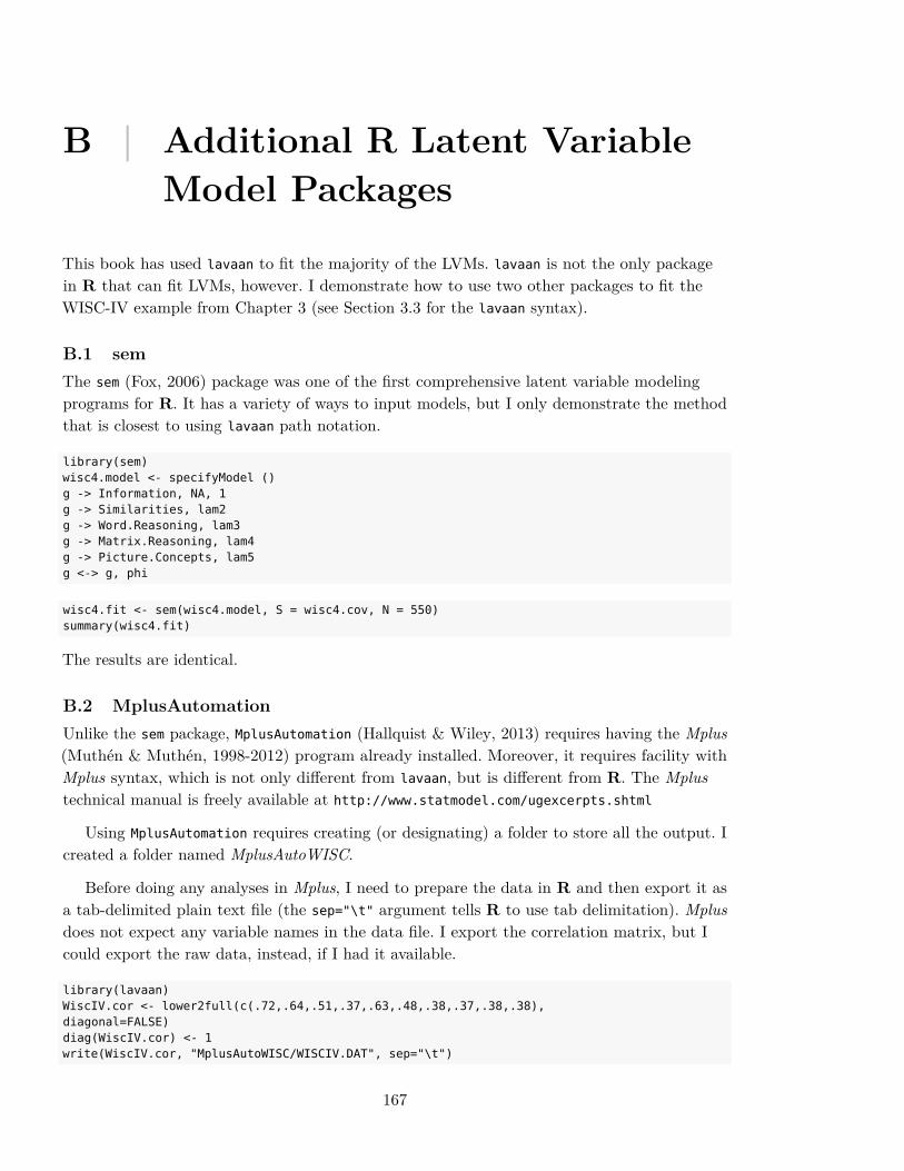
B | Additional R Latent VariableModel Packages
This book has used lavaan to fit the majority of the LVMs. lavaan is not the only packagein R that can fit LVMs, however. I demonstrate how to use two other packages to fit theWISC-IV example from Chapter 3 (see Section 3.3 for the lavaan syntax).
B.1 semThe sem (Fox, 2006) package was one of the first comprehensive latent variable modelingprograms for R. It has a variety of ways to input models, but I only demonstrate the methodthat is closest to using lavaan path notation.
library(sem)wisc4.model <- specifyModel ()g -> Information, NA, 1g -> Similarities, lam2g -> Word.Reasoning, lam3g -> Matrix.Reasoning, lam4g -> Picture.Concepts, lam5g <-> g, phi
wisc4.fit <- sem(wisc4.model, S = wisc4.cov, N = 550)summary(wisc4.fit)
The results are identical.
B.2 MplusAutomationUnlike the sem package, MplusAutomation (Hallquist & Wiley, 2013) requires having the Mplus(Muthén & Muthén, 1998-2012) program already installed. Moreover, it requires facility withMplus syntax, which is not only different from lavaan, but is different from R. The Mplustechnical manual is freely available at http://www.statmodel.com/ugexcerpts.shtml
Using MplusAutomation requires creating (or designating) a folder to store all the output. Icreated a folder named MplusAutoWISC.
Before doing any analyses in Mplus, I need to prepare the data in R and then export it asa tab-delimited plain text file (the sep="\t" argument tells R to use tab delimitation). Mplusdoes not expect any variable names in the data file. I export the correlation matrix, but Icould export the raw data, instead, if I had it available.
library(lavaan)WiscIV.cor <- lower2full(c(.72,.64,.51,.37,.63,.48,.38,.37,.38,.38),diagonal=FALSE)diag(WiscIV.cor) <- 1write(WiscIV.cor, "MplusAutoWISC/WISCIV.DAT", sep="\t")
167
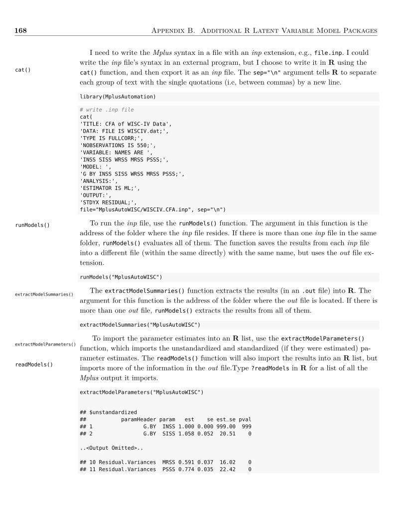
168 Appendix B. Additional R Latent Variable Model Packages
cat()
runModels()
extractModelSummaries()
extractModelParameters()
readModels()
I need to write the Mplus syntax in a file with an inp extension, e.g., file.inp. I couldwrite the inp file’s syntax in an external program, but I choose to write it in R using thecat() function, and then export it as an inp file. The sep="\n" argument tells R to separateeach group of text with the single quotations (i.e, between commas) by a new line.
library(MplusAutomation)
# write .inp filecat('TITLE: CFA of WISC-IV Data','DATA: FILE IS WISCIV.dat;','TYPE IS FULLCORR;','NOBSERVATIONS IS 550;','VARIABLE: NAMES ARE ','INSS SISS WRSS MRSS PSSS;','MODEL: ','G BY INSS SISS WRSS MRSS PSSS;','ANALYSIS:','ESTIMATOR IS ML;','OUTPUT:','STDYX RESIDUAL;',file="MplusAutoWISC/WISCIV_CFA.inp", sep="\n")
To run the inp file, use the runModels() function. The argument in this function is theaddress of the folder where the inp file resides. If there is more than one inp file in the samefolder, runModels() evaluates all of them. The function saves the results from each inp fileinto a different file (within the same directly) with the same name, but uses the out file ex-tension.
runModels("MplusAutoWISC")
The extractModelSummaries() function extracts the results (in an .out file) into R. Theargument for this function is the address of the folder where the out file is located. If there ismore than one out file, runModels() extracts the results from all of them.
extractModelSummaries("MplusAutoWISC")
To import the parameter estimates into an R list, use the extractModelParameters()
function, which imports the unstandardized and standardized (if they were estimated) pa-rameter estimates. The readModels() function will also import the results into an R list, butimports more of the information in the out file.Type ?readModels in R for a list of all theMplus output it imports.
extractModelParameters("MplusAutoWISC")
## $unstandardized## paramHeader param est se est_se pval## 1 G.BY INSS 1.000 0.000 999.00 999## 2 G.BY SISS 1.058 0.052 20.51 0
..<Output Omitted>..
## 10 Residual.Variances MRSS 0.591 0.037 16.02 0## 11 Residual.Variances PSSS 0.774 0.035 22.42 0
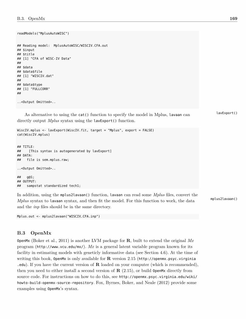
B.3. OpenMx 169
readModels("MplusAutoWISC")
## Reading model: MplusAutoWISC/WISCIV_CFA.out## $input## $title## [1] "CFA of WISC-IV Data"#### $data## $data$file## [1] "WISCIV.dat"#### $data$type## [1] "FULLCORR"##
..<Output Omitted>..
As alternative to using the cat() function to specify the model in Mplus, lavaan candirectly output Mplus syntax using the lavExport() function.
WiscIV.mplus <- lavExport(WiscIV.fit, target = "Mplus", export = FALSE)cat(WiscIV.mplus)
## TITLE:## [This syntax is autogenerated by lavExport]## DATA:## file is sem.mplus.raw;
..<Output Omitted>..
## g@1;## OUTPUT:## sampstat standardized tech1;
In addition, using the mplus2lavaan() function, lavaan can read some Mplus files, convert theMplus syntax to lavaan syntax, and then fit the model. For this function to work, the dataand the inp files should be in the same directory.
Mplus.out <- mplus2lavaan("WISCIV_CFA.inp")
B.3 OpenMxOpenMx (Boker et al., 2011) is another LVM package for R, built to extend the original Mxprogram (http://www.vcu.edu/mx/). Mx is a general latent variable program known for itsfacility in estimating models with geneticly informative data (see Section 4.6). At the time ofwriting this book, OpenMx is only available for R version 2.15 (http://openmx.psyc.virginia.edu). If you have the current version of R loaded on your computer (which is recommended),then you need to either install a second version of R (2.15), or build OpenMx directly fromsource code. For instructions on how to do this, see http://openmx.psyc.virginia.edu/wiki/
howto-build-openmx-source-repository. Fox, Byrnes, Boker, and Neale (2012) provide someexamples using OpenMx’s syntax.
lavExport()
mplus2lavaan()
170 Appendix B. Additional R Latent Variable Model Packages
B.4 ReferencesBoker, S. M., Neale, M. C., Maes, H. H. M., Wilde, M., Spiegel, M., Brick, T., . . . Fox, J.
(2011). OpenMx: An open source extended structural equation modeling framework.Psychometrika, 76 , 306-317. doi: 10.1007/s11336-010-9200-6
Fox, J. (2006). Teacher’s corner: Structural equation modeling with the sem package in R.Structural Equation Modeling: A Multidisciplinary Journal, 13 , 465-486. doi:10.1207/s15328007sem1303_7
Fox, J., Byrnes, J. E., Boker, S. M., & Neale, M. C. (2012). Structural equation modeling in Rwith the sem and OpenMx packages. In R. H. Hoyle (Ed.), Handbook of structuralequation modeling (pp. 325–340). New York, NY: Guilford.
Hallquist, M., & Wiley, J. (2013). MplusAutomation: Automating Mplus model estimation andinterpretation [Computer program]. Retrieved fromhttp://CRAN.R-project.org/package=MplusAutomation.
Muthén, L. K., & Muthén, B. O. (1998-2012). Mplus user’s guide (7th ed.). Los Angeles, CA:Author
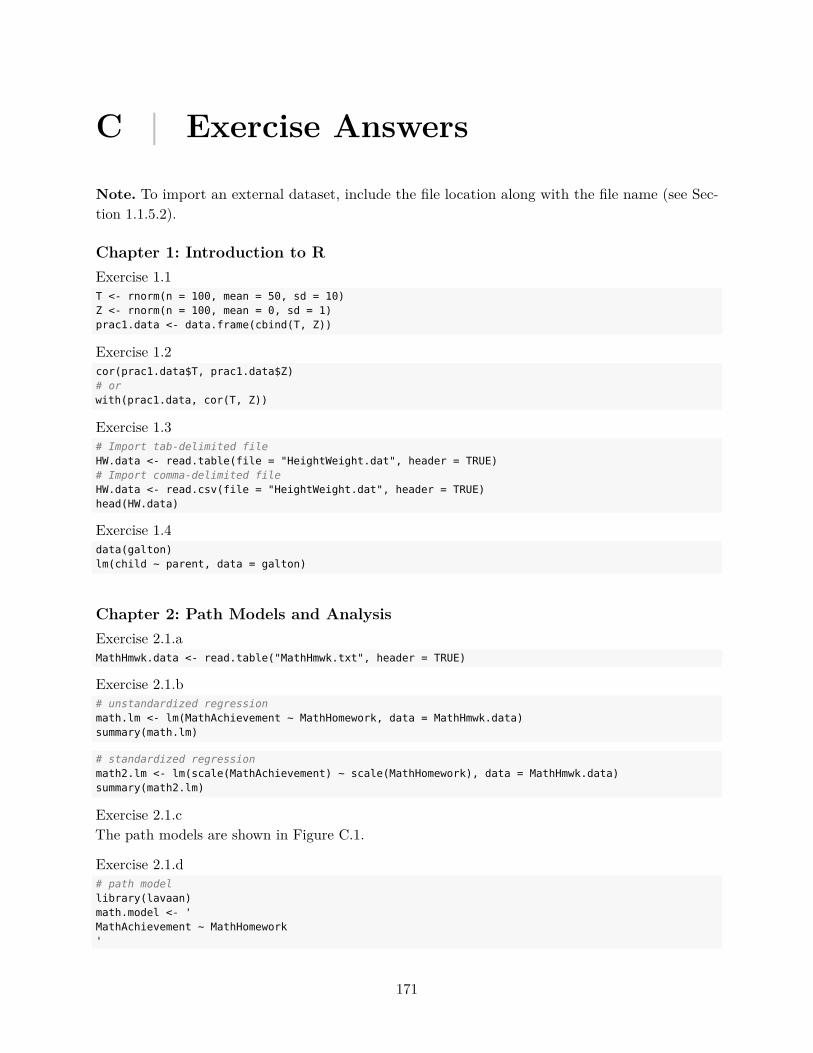
C | Exercise Answers
Note. To import an external dataset, include the file location along with the file name (see Sec-tion 1.1.5.2).
Chapter 1: Introduction to RExercise 1.1T <- rnorm(n = 100, mean = 50, sd = 10)Z <- rnorm(n = 100, mean = 0, sd = 1)prac1.data <- data.frame(cbind(T, Z))
Exercise 1.2cor(prac1.data$T, prac1.data$Z)# orwith(prac1.data, cor(T, Z))
Exercise 1.3# Import tab-delimited fileHW.data <- read.table(file = "HeightWeight.dat", header = TRUE)# Import comma-delimited fileHW.data <- read.csv(file = "HeightWeight.dat", header = TRUE)head(HW.data)
Exercise 1.4data(galton)lm(child ~ parent, data = galton)
Chapter 2: Path Models and AnalysisExercise 2.1.aMathHmwk.data <- read.table("MathHmwk.txt", header = TRUE)
Exercise 2.1.b# unstandardized regressionmath.lm <- lm(MathAchievement ~ MathHomework, data = MathHmwk.data)summary(math.lm)
# standardized regressionmath2.lm <- lm(scale(MathAchievement) ~ scale(MathHomework), data = MathHmwk.data)summary(math2.lm)
Exercise 2.1.cThe path models are shown in Figure C.1.
Exercise 2.1.d# path modellibrary(lavaan)math.model <- 'MathAchievement ~ MathHomework'
171
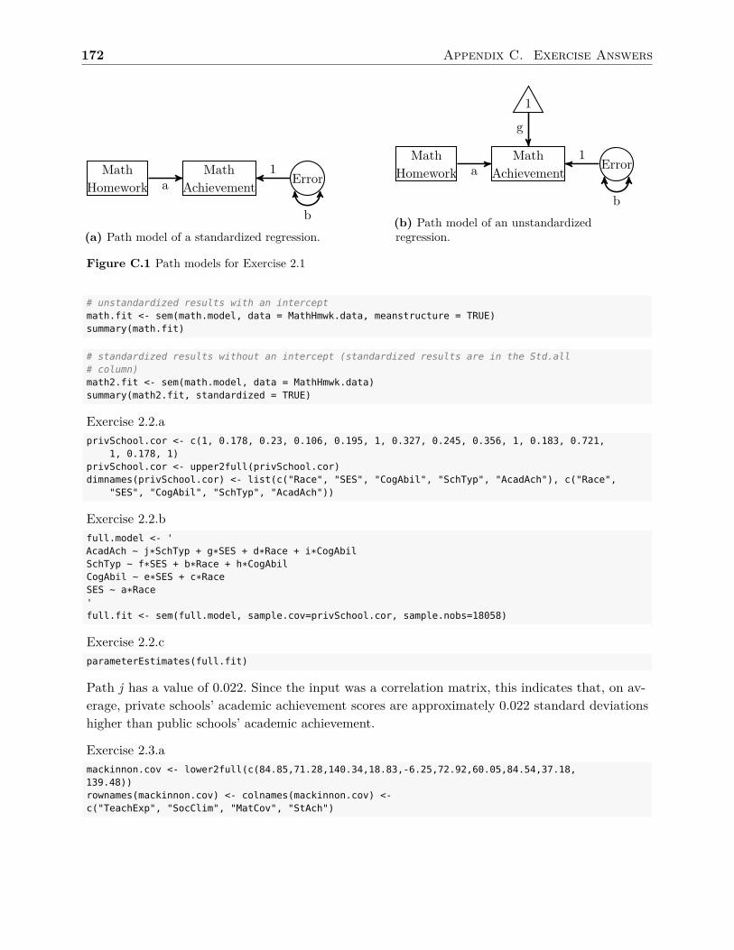
172 Appendix C. Exercise Answers
MathHomework
MathAchievement Error
b
a1
(a) Path model of a standardized regression.
MathHomework
MathAchievement Error
1
b
a1
g
(b) Path model of an unstandardizedregression.
Figure C.1 Path models for Exercise 2.1
# unstandardized results with an interceptmath.fit <- sem(math.model, data = MathHmwk.data, meanstructure = TRUE)summary(math.fit)
# standardized results without an intercept (standardized results are in the Std.all# column)math2.fit <- sem(math.model, data = MathHmwk.data)summary(math2.fit, standardized = TRUE)
Exercise 2.2.aprivSchool.cor <- c(1, 0.178, 0.23, 0.106, 0.195, 1, 0.327, 0.245, 0.356, 1, 0.183, 0.721,
1, 0.178, 1)privSchool.cor <- upper2full(privSchool.cor)dimnames(privSchool.cor) <- list(c("Race", "SES", "CogAbil", "SchTyp", "AcadAch"), c("Race",
"SES", "CogAbil", "SchTyp", "AcadAch"))
Exercise 2.2.bfull.model <- 'AcadAch ~ j*SchTyp + g*SES + d*Race + i*CogAbilSchTyp ~ f*SES + b*Race + h*CogAbilCogAbil ~ e*SES + c*RaceSES ~ a*Race'full.fit <- sem(full.model, sample.cov=privSchool.cor, sample.nobs=18058)
Exercise 2.2.cparameterEstimates(full.fit)
Path j has a value of 0.022. Since the input was a correlation matrix, this indicates that, on av-erage, private schools’ academic achievement scores are approximately 0.022 standard deviationshigher than public schools’ academic achievement.
Exercise 2.3.amackinnon.cov <- lower2full(c(84.85,71.28,140.34,18.83,-6.25,72.92,60.05,84.54,37.18,139.48))rownames(mackinnon.cov) <- colnames(mackinnon.cov) <-c("TeachExp", "SocClim", "MatCov", "StAch")
Appendix C. Exercise Answers 173
Exercise 2.3.bmackinnon.model <- 'StAch ~ b1*SocClim + b2*MatCov + c*TeachExpMatCov ~ a2*TeachExpSocClim ~ a1*TeachExpind1 := a1*b1ind2 := a2*b2'
Exercise 2.3.cmackinnon.fit <- sem(mackinnon.model, sample.cov = mackinnon.cov, sample.nobs = 40)summary(mackinnon.fit, standardized = TRUE)
The indirect effect through social climate is 0.478. The indirect effect through material covered is0.118.
Chapter 3: Basic Latent Variable ModelsExercise 3.1.apsychSoc.cov <- c(0.77, 0.38, 0.65, 0.39, 0.39, 0.62, -0.25, -0.32, -0.27, 6.09)psychSoc.cov <- lower2full(psychSoc.cov)rownames(psychSoc.cov) <- colnames(psychSoc.cov) <- c("Dep.1", "Dep.2", "Dep.3", "SocActivity")
Exercise 3.1.b# marker variablemarker.model <- 'PsychSocLV =~ Dep.1 + Dep.2 + Dep.3 + SocActivity'marker.fit <- cfa(marker.model, sample.cov=psychSoc.cov, sample.nobs=6053)
# standardized latent variable## method 1stdLV.fit1 <- cfa(marker.model, sample.cov=psychSoc.cov, std.lv=TRUE, sample.nobs=6053)## method 2stdLV.model <- 'PsychSocLV =~ NA*Dep.1 + Dep.1 + Dep.2 + Dep.3 + SocActivityPsychSocLV~~1*PsychSocLV'stdLV.fit2 <- cfa(stdLV.model, sample.cov=psychSoc.cov, sample.nobs=6053)
# effects-codingec.model <- 'PsychSocLV =~ NA*Dep.1 + a*Dep.1 + b*Dep.2 + c*Dep.3 + d*SocActivitya+b+c+d==4'ec.fit <- cfa(ec.model, sample.cov=psychSoc.cov, sample.nobs=6053)
Exercise 3.2.amobility.cov <- c(0.77 , 0.38 , 0.65 , 0.39 , 0.39 , 0.62, -0.25, -0.32, -0.27 , 6.09, 0.31,0.29 , 0.26, -0.36 , 7.67 , 0.24 , 0.25 , 0.19, -0.18, 0.51, 1.69, -3.16, -3.56, -2.63 , 6.09,-3.12, -4.58, 204.79, -0.92, -0.88, -0.72 , 0.88, -1.49, -1.41, 16.53, 7.24)
mobility.cov <- lower2full(mobility.cov)rownames(mobility.cov) <- colnames(mobility.cov) <- c("Dep.1", "Dep.2", "Dep.3", "SocActivity","Falls", "Chronic", "TotActivity", "PersMobility")
174 Appendix C. Exercise Answers
Exercise 3.2.bmobility.model <- 'PsychSocLV =~ Dep.1 + Dep.2 + Dep.3 + SocActivityPsyHealthLV =~ Falls + Chronic + TotActivityPersMobility ~ PsychSocLV + PsyHealthLV'mobility.fit <- sem(mobility.model, sample.cov=mobility.cov, sample.nobs=6053)summary(mobility.fit, fit.measures=TRUE, standardized=TRUE)
Physical health (-0.914) appears to be a stronger predictor of personal mobility than psychosocialhealth (0.101).
Exercise 3.3.adda.cov <- lower2full(c(59.66, 11.18, 22.3, 2.63, 0.41, 1), diagonal = TRUE)rownames(dda.cov) <- colnames(dda.cov) <- c("DV1", "DV2", "Cat1")
Exercise 3.3.bdda.model<-'F1 <~ 1*DV1 + a*DV1 + b*DV2Cat1 ~ c*F1Cat1~~d*Cat1'
Exercise 3.3.cdda.fit <- sem(dda.model, sample.cov = dda.cov, sample.nobs = 288)parameterEstimates(dda.fit, standardized = TRUE)
The function coefficients are 1.016 (a) and -0.057 (b), the canonical correlation is 0.341 (c), andR
2 is 0.116 (i.e., 1− 0.884)
Chapter 4: Latent Variable Models with Multiple GroupsExercise 4.1.a# WISCWISC1.names <- c("Comp", "Arith", "Sim","Voc","DigSp","PicComp","BlkDsgn","Cod")
WISC1_7yo.cor<-c(1, 0.31, 1, 0.36, 0.4, 1, 0.51, 0.46, 0.45, 1, 0.29, 0.4, 0.33, 0.43, 1, 0.39,0.29, 0.27, 0.36, 0.33, 1, 0.32, 0.27, 0.29, 0.33, 0.24, 0.28, 1, 0.22, 0.32, 0.15, 0.22,
0.27, 0.12, 0.26, 1)WISC1_7yo.cor<-lower2full(WISC1_7yo.cor)rownames(WISC1_7yo.cor)<-colnames(WISC1_7yo.cor)<-WISC1.namesWISC1_7yo.mean<-c(7.83, 5.50, 5.67, 21.50, 7.67, 8.00, 6.50, 34.83)WISC1_7yo.SD<-c(2.69, 1.50, 2.36, 6.06, 1.85, 2.18, 5.97, 9.94)WISC1_7yo.cov<-cor2cov(WISC1_7yo.cor, WISC1_7yo.SD)names(WISC1_7yo.mean)<-WISC1.namesnames(WISC1_7yo.SD)<-WISC1.names
# WISC-RWISC2.names<-c("Sim", "Arith", "Voc", "Comp", "DigSp","PicComp","BlkDsgn","Cod")
WISC2_7yo.cor<-c(1, 0.43, 1, 0.59, 0.5, 1, 0.45, 0.43, 0.61, 1, 0.34, 0.47, 0.35, 0.34, 1, 0.36,0.25, 0.37, 0.33, 0.18, 1, 0.5, 0.42, 0.43, 0.43, 0.32, 0.42, 1, 0.18, 0.22, 0.27, 0.18,0.18, 0.13, 0.26, 1)WISC2_7yo.cor<-lower2full(WISC2_7yo.cor)rownames(WISC2_7yo.cor)<-colnames(WISC2_7yo.cor)<-WISC2.namesWISC2_7yo.mean<-c(8.33, 7.83, 19.67, 11.00, 8.67, 13.67, 12.00, 39.00)
Appendix C. Exercise Answers 175
WISC2_7yo.SD<-c(3.26, 1.77, 5.07, 3.63, 2.86, 4.25, 8.82, 8.05)WISC2_7yo.cov<-cor2cov(WISC2_7yo.cor, WISC2_7yo.SD)names(WISC2_7yo.mean)<-WISC2.namesnames(WISC2_7yo.SD)<-WISC2.names
# WISC-IIIWISC3.names<-c("Sim", "Arith", "Voc", "Comp", "DigSp","PicComp","Cod","BlkDsgn")
WISC3_7yo.cor<-c(1.00, 0.46, 1.00, 0.64, 0.41, 1.00, 0.46, 0.33, 0.61, 1.00, 0.36, 0.39, 0.30,0.22, 1.00, 0.33, 0.30, 0.31, 0.23, 0.25, 1.00, 0.18, 0.22, 0.19, 0.13, 0.09, 0.24, 1.00,
0.37, 0.36, 0.35, 0.22, 0.30, 0.47, 0.20, 1.00)WISC3_7yo.cor<-lower2full(WISC3_7yo.cor)rownames(WISC3_7yo.cor)<-colnames(WISC3_7yo.cor)<-WISC3.namesWISC3_7yo.mean <- c(10.00, 12.83, 17.00, 12.50, 10.50, 13.67, 43.67, 18.67)WISC3_7yo.SD <- c(3.19, 2.19, 4.76, 3.52, 2.53, 3.85, 10.51, 10.25)WISC3_7yo.cov<-cor2cov(WISC3_7yo.cor, WISC3_7yo.SD)names(WISC3_7yo.mean)<-WISC3.namesnames(WISC3_7yo.SD)<-WISC3.names
# WISC-IVWISC4.names<-c("BlkDsgn", "Sim", "DigSp", "Cod", "Voc", "Comp", "PicComp", "Arith")
WISC4_7yo.cor <- c(1.00, 0.49, 1.00, 0.29, 0.37, 1.00, 0.23, 0.16, 0.12, 1.00, 0.41, 0.73, 0.33,0.09, 1.00, 0.33, 0.58, 0.27, 0.15, 0.63, 1.00, 0.43, 0.37, 0.13, 0.25, 0.43, 0.45, 1.00,0.52, 0.55, 0.51, 0.27, 0.43, 0.46, 0.38, 1.00)WISC4_7yo.cor <- lower2full(WISC4_7yo.cor)rownames(WISC4_7yo.cor)<-colnames(WISC4_7yo.cor)<-WISC4.namesWISC4_7yo.mean <- c(18.67, 11.83, 12.17, 45.83, 21.67, 15.17, 17.83, 15.00)WISC4_7yo.SD <- c(9.36, 5.20, 2.72, 10.44, 6.54, 4.93, 5.35, 4.10)WISC4_7yo.cov<-cor2cov(WISC4_7yo.cor, WISC4_7yo.SD)names(WISC4_7yo.mean)<-WISC4.namesnames(WISC4_7yo.SD)<-WISC4.names
# Combine the covarainces, means, and sample sizesWISC_7yo.cov <- list(WISC1=WISC1_7yo.cov, WISC2=WISC2_7yo.cov, WISC3=WISC3_7yo.cov,WISC4=WISC4_7yo.cov)WISC_7yo.mean <- list(WISC1=WISC1_7yo.mean, WISC2=WISC2_7yo.mean,WISC3=WISC3_7yo.mean,WISC4=WISC4_7yo.mean)WISC_7yo.n <- list(WISC1=200, WISC2=200,WISC3=200, WISC4=200)
Exercise 4.1.b# Beaujean & Sheng's final model with partial invarianceWISC_7yo.model<-'WISC1:g =~ co1*Comp + ar1*Arith + si1*Sim + vo1*Voc + DigSp + pc1*PicComp + bd1*BlkDsgn + CodComp ~~ Voc + PicCompBlkDsgn~bd1.i*1Comp~co1.i*1PicComp~pc1.i*1Arith~ar1.i*1Voc~vo1.i*1
WISC2:g =~ co2*Comp + ar2*Arith + si2*Sim + vo2*Voc + DigSp + pc2*PicComp + BlkDsgn + CodDigSp ~~ ArithBlkDsgn ~~ Voc
g~g2*1Arith~ar2.i*1
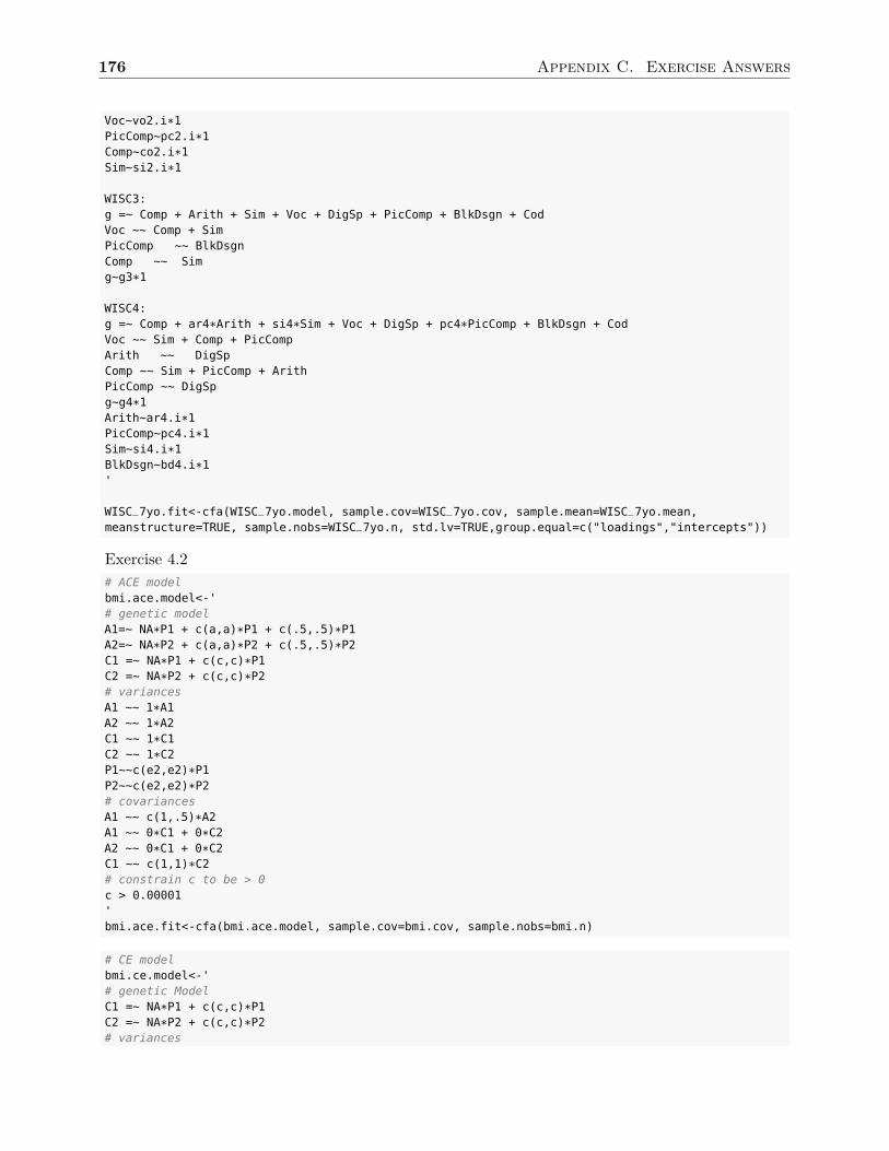
176 Appendix C. Exercise Answers
Voc~vo2.i*1PicComp~pc2.i*1Comp~co2.i*1Sim~si2.i*1
WISC3:g =~ Comp + Arith + Sim + Voc + DigSp + PicComp + BlkDsgn + CodVoc ~~ Comp + SimPicComp ~~ BlkDsgnComp ~~ Simg~g3*1
WISC4:g =~ Comp + ar4*Arith + si4*Sim + Voc + DigSp + pc4*PicComp + BlkDsgn + CodVoc ~~ Sim + Comp + PicCompArith ~~ DigSpComp ~~ Sim + PicComp + ArithPicComp ~~ DigSpg~g4*1Arith~ar4.i*1PicComp~pc4.i*1Sim~si4.i*1BlkDsgn~bd4.i*1'
WISC_7yo.fit<-cfa(WISC_7yo.model, sample.cov=WISC_7yo.cov, sample.mean=WISC_7yo.mean,meanstructure=TRUE, sample.nobs=WISC_7yo.n, std.lv=TRUE,group.equal=c("loadings","intercepts"))
Exercise 4.2# ACE modelbmi.ace.model<-'# genetic modelA1=~ NA*P1 + c(a,a)*P1 + c(.5,.5)*P1A2=~ NA*P2 + c(a,a)*P2 + c(.5,.5)*P2C1 =~ NA*P1 + c(c,c)*P1C2 =~ NA*P2 + c(c,c)*P2# variancesA1 ~~ 1*A1A2 ~~ 1*A2C1 ~~ 1*C1C2 ~~ 1*C2P1~~c(e2,e2)*P1P2~~c(e2,e2)*P2# covariancesA1 ~~ c(1,.5)*A2A1 ~~ 0*C1 + 0*C2A2 ~~ 0*C1 + 0*C2C1 ~~ c(1,1)*C2# constrain c to be > 0c > 0.00001'bmi.ace.fit<-cfa(bmi.ace.model, sample.cov=bmi.cov, sample.nobs=bmi.n)
# CE modelbmi.ce.model<-'# genetic ModelC1 =~ NA*P1 + c(c,c)*P1C2 =~ NA*P2 + c(c,c)*P2# variances
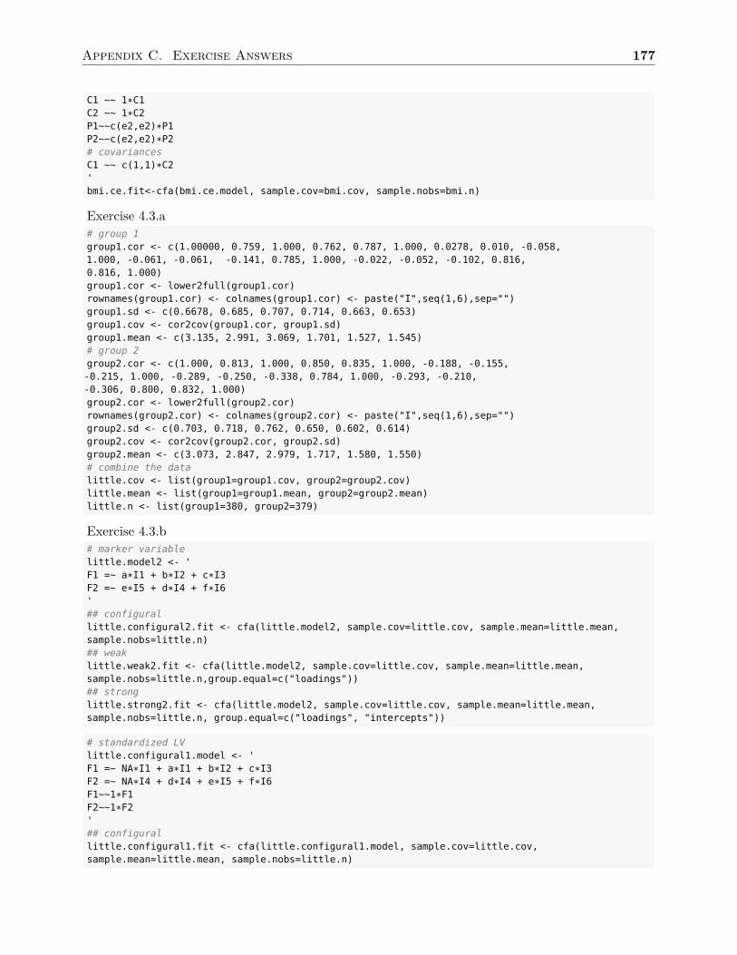
Appendix C. Exercise Answers 177
C1 ~~ 1*C1C2 ~~ 1*C2P1~~c(e2,e2)*P1P2~~c(e2,e2)*P2# covariancesC1 ~~ c(1,1)*C2'bmi.ce.fit<-cfa(bmi.ce.model, sample.cov=bmi.cov, sample.nobs=bmi.n)
Exercise 4.3.a# group 1group1.cor <- c(1.00000, 0.759, 1.000, 0.762, 0.787, 1.000, 0.0278, 0.010, -0.058,1.000, -0.061, -0.061, -0.141, 0.785, 1.000, -0.022, -0.052, -0.102, 0.816,0.816, 1.000)group1.cor <- lower2full(group1.cor)rownames(group1.cor) <- colnames(group1.cor) <- paste("I",seq(1,6),sep="")group1.sd <- c(0.6678, 0.685, 0.707, 0.714, 0.663, 0.653)group1.cov <- cor2cov(group1.cor, group1.sd)group1.mean <- c(3.135, 2.991, 3.069, 1.701, 1.527, 1.545)# group 2group2.cor <- c(1.000, 0.813, 1.000, 0.850, 0.835, 1.000, -0.188, -0.155,-0.215, 1.000, -0.289, -0.250, -0.338, 0.784, 1.000, -0.293, -0.210,-0.306, 0.800, 0.832, 1.000)group2.cor <- lower2full(group2.cor)rownames(group2.cor) <- colnames(group2.cor) <- paste("I",seq(1,6),sep="")group2.sd <- c(0.703, 0.718, 0.762, 0.650, 0.602, 0.614)group2.cov <- cor2cov(group2.cor, group2.sd)group2.mean <- c(3.073, 2.847, 2.979, 1.717, 1.580, 1.550)# combine the datalittle.cov <- list(group1=group1.cov, group2=group2.cov)little.mean <- list(group1=group1.mean, group2=group2.mean)little.n <- list(group1=380, group2=379)
Exercise 4.3.b# marker variablelittle.model2 <- 'F1 =~ a*I1 + b*I2 + c*I3F2 =~ e*I5 + d*I4 + f*I6'## configurallittle.configural2.fit <- cfa(little.model2, sample.cov=little.cov, sample.mean=little.mean,sample.nobs=little.n)## weaklittle.weak2.fit <- cfa(little.model2, sample.cov=little.cov, sample.mean=little.mean,sample.nobs=little.n,group.equal=c("loadings"))## stronglittle.strong2.fit <- cfa(little.model2, sample.cov=little.cov, sample.mean=little.mean,sample.nobs=little.n, group.equal=c("loadings", "intercepts"))
# standardized LVlittle.configural1.model <- 'F1 =~ NA*I1 + a*I1 + b*I2 + c*I3F2 =~ NA*I4 + d*I4 + e*I5 + f*I6F1~~1*F1F2~~1*F2'## configurallittle.configural1.fit <- cfa(little.configural1.model, sample.cov=little.cov,sample.mean=little.mean, sample.nobs=little.n)
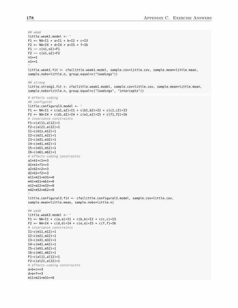
178 Appendix C. Exercise Answers
## weaklittle.weak1.model <- 'F1 =~ NA*I1 + a*I1 + b*I2 + c*I3F2 =~ NA*I4 + d*I4 + e*I5 + f*I6F1 ~~ c(n1,n2)*F1F2 ~~ c(o1,o2)*F2n1==1o1==1'little.weak1.fit <- cfa(little.weak1.model, sample.cov=little.cov, sample.mean=little.mean,sample.nobs=little.n, group.equal=c("loadings"))
## stronglittle.strong1.fit <- cfa(little.weak1.model, sample.cov=little.cov, sample.mean=little.mean,sample.nobs=little.n, group.equal=c("loadings", "intercepts"))
# effects coding## configurallittle.configural3.model <- 'F1 =~ NA*I1 + c(a1,a2)*I1 + c(b1,b2)*I2 + c(c1,c2)*I3F2 =~ NA*I4 + c(d1,d2)*I4 + c(e1,e2)*I5 + c(f1,f2)*I6# invariance constraintsF1~c(al11,al12)*1F2~c(al21,al22)*1I1~c(m11,m12)*1I2~c(m21,m22)*1I3~c(m31,m32)*1I4~c(m41,m42)*1I5~c(m51,m52)*1I6~c(m61,m62)*1# effects-coding constraintsa1+b1+c1==3d1+e1+f1==3a2+b2+c2==3d2+b2+f2==3m11+m21+m31==0m41+m51+m61==0m12+m22+m32==0m42+m52+m62==0'little.configural3.fit <- cfa(little.configural3.model, sample.cov=little.cov,sample.mean=little.mean, sample.nobs=little.n)
## weaklittle.weak3.model <- 'F1 =~ NA*I1 + c(a,a)*I1 + c(b,b)*I2 + c(c,c)*I3F2 =~ NA*I4 + c(d,d)*I4 + c(e,e)*I5 + c(f,f)*I6# invariance constraintsI1~c(m11,m12)*1I2~c(m21,m22)*1I3~c(m31,m32)*1I4~c(m41,m42)*1I5~c(m51,m52)*1I6~c(m61,m62)*1F1~c(al11,al12)*1F2~c(al21,al22)*1# effects-coding constraintsa+b+c==3d+e+f==3m11+m21+m31==0
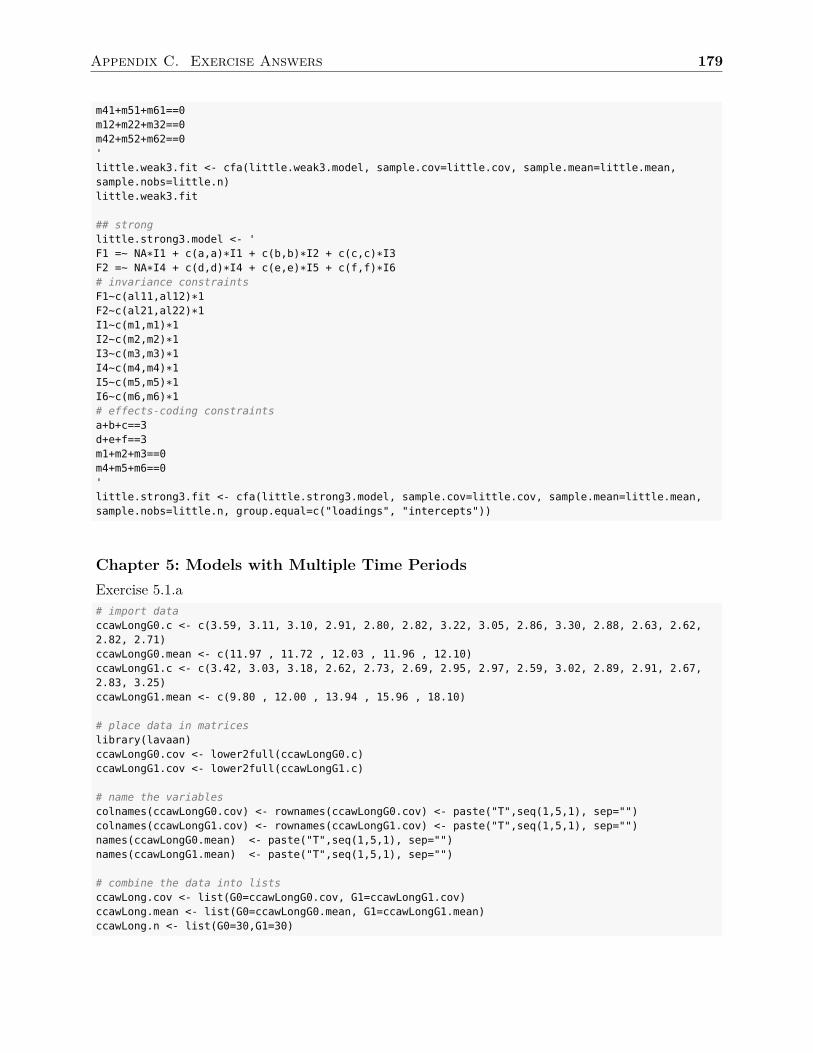
Appendix C. Exercise Answers 179
m41+m51+m61==0m12+m22+m32==0m42+m52+m62==0'little.weak3.fit <- cfa(little.weak3.model, sample.cov=little.cov, sample.mean=little.mean,sample.nobs=little.n)little.weak3.fit
## stronglittle.strong3.model <- 'F1 =~ NA*I1 + c(a,a)*I1 + c(b,b)*I2 + c(c,c)*I3F2 =~ NA*I4 + c(d,d)*I4 + c(e,e)*I5 + c(f,f)*I6# invariance constraintsF1~c(al11,al12)*1F2~c(al21,al22)*1I1~c(m1,m1)*1I2~c(m2,m2)*1I3~c(m3,m3)*1I4~c(m4,m4)*1I5~c(m5,m5)*1I6~c(m6,m6)*1# effects-coding constraintsa+b+c==3d+e+f==3m1+m2+m3==0m4+m5+m6==0'little.strong3.fit <- cfa(little.strong3.model, sample.cov=little.cov, sample.mean=little.mean,sample.nobs=little.n, group.equal=c("loadings", "intercepts"))
Chapter 5: Models with Multiple Time PeriodsExercise 5.1.a# import dataccawLongG0.c <- c(3.59, 3.11, 3.10, 2.91, 2.80, 2.82, 3.22, 3.05, 2.86, 3.30, 2.88, 2.63, 2.62,2.82, 2.71)ccawLongG0.mean <- c(11.97 , 11.72 , 12.03 , 11.96 , 12.10)ccawLongG1.c <- c(3.42, 3.03, 3.18, 2.62, 2.73, 2.69, 2.95, 2.97, 2.59, 3.02, 2.89, 2.91, 2.67,2.83, 3.25)ccawLongG1.mean <- c(9.80 , 12.00 , 13.94 , 15.96 , 18.10)
# place data in matriceslibrary(lavaan)ccawLongG0.cov <- lower2full(ccawLongG0.c)ccawLongG1.cov <- lower2full(ccawLongG1.c)
# name the variablescolnames(ccawLongG0.cov) <- rownames(ccawLongG0.cov) <- paste("T",seq(1,5,1), sep="")colnames(ccawLongG1.cov) <- rownames(ccawLongG1.cov) <- paste("T",seq(1,5,1), sep="")names(ccawLongG0.mean) <- paste("T",seq(1,5,1), sep="")names(ccawLongG1.mean) <- paste("T",seq(1,5,1), sep="")
# combine the data into listsccawLong.cov <- list(G0=ccawLongG0.cov, G1=ccawLongG1.cov)ccawLong.mean <- list(G0=ccawLongG0.mean, G1=ccawLongG1.mean)ccawLong.n <- list(G0=30,G1=30)
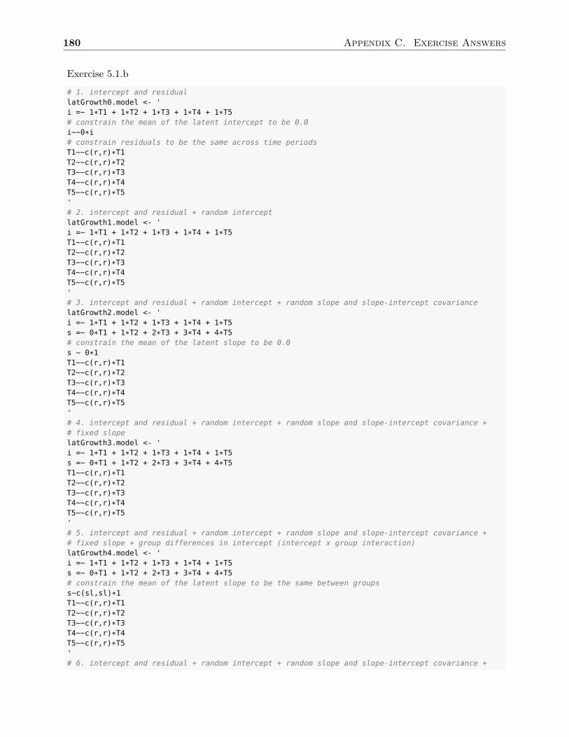
180 Appendix C. Exercise Answers
Exercise 5.1.b
# 1. intercept and residuallatGrowth0.model <- 'i =~ 1*T1 + 1*T2 + 1*T3 + 1*T4 + 1*T5# constrain the mean of the latent intercept to be 0.0i~~0*i# constrain residuals to be the same across time periodsT1~~c(r,r)*T1T2~~c(r,r)*T2T3~~c(r,r)*T3T4~~c(r,r)*T4T5~~c(r,r)*T5'# 2. intercept and residual + random interceptlatGrowth1.model <- 'i =~ 1*T1 + 1*T2 + 1*T3 + 1*T4 + 1*T5T1~~c(r,r)*T1T2~~c(r,r)*T2T3~~c(r,r)*T3T4~~c(r,r)*T4T5~~c(r,r)*T5'# 3. intercept and residual + random intercept + random slope and slope-intercept covariancelatGrowth2.model <- 'i =~ 1*T1 + 1*T2 + 1*T3 + 1*T4 + 1*T5s =~ 0*T1 + 1*T2 + 2*T3 + 3*T4 + 4*T5# constrain the mean of the latent slope to be 0.0s ~ 0*1T1~~c(r,r)*T1T2~~c(r,r)*T2T3~~c(r,r)*T3T4~~c(r,r)*T4T5~~c(r,r)*T5'# 4. intercept and residual + random intercept + random slope and slope-intercept covariance +# fixed slopelatGrowth3.model <- 'i =~ 1*T1 + 1*T2 + 1*T3 + 1*T4 + 1*T5s =~ 0*T1 + 1*T2 + 2*T3 + 3*T4 + 4*T5T1~~c(r,r)*T1T2~~c(r,r)*T2T3~~c(r,r)*T3T4~~c(r,r)*T4T5~~c(r,r)*T5'# 5. intercept and residual + random intercept + random slope and slope-intercept covariance +# fixed slope + group differences in intercept (intercept x group interaction)latGrowth4.model <- 'i =~ 1*T1 + 1*T2 + 1*T3 + 1*T4 + 1*T5s =~ 0*T1 + 1*T2 + 2*T3 + 3*T4 + 4*T5# constrain the mean of the latent slope to be the same between groupss~c(sl,sl)*1T1~~c(r,r)*T1T2~~c(r,r)*T2T3~~c(r,r)*T3T4~~c(r,r)*T4T5~~c(r,r)*T5'# 6. intercept and residual + random intercept + random slope and slope-intercept covariance +
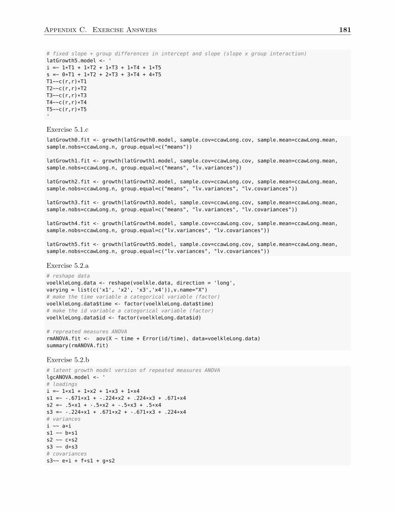
Appendix C. Exercise Answers 181
# fixed slope + group differences in intercept and slope (slope x group interaction)latGrowth5.model <- 'i =~ 1*T1 + 1*T2 + 1*T3 + 1*T4 + 1*T5s =~ 0*T1 + 1*T2 + 2*T3 + 3*T4 + 4*T5T1~~c(r,r)*T1T2~~c(r,r)*T2T3~~c(r,r)*T3T4~~c(r,r)*T4T5~~c(r,r)*T5'
Exercise 5.1.clatGrowth0.fit <- growth(latGrowth0.model, sample.cov=ccawLong.cov, sample.mean=ccawLong.mean,sample.nobs=ccawLong.n, group.equal=c("means"))
latGrowth1.fit <- growth(latGrowth1.model, sample.cov=ccawLong.cov, sample.mean=ccawLong.mean,sample.nobs=ccawLong.n, group.equal=c("means", "lv.variances"))
latGrowth2.fit <- growth(latGrowth2.model, sample.cov=ccawLong.cov, sample.mean=ccawLong.mean,sample.nobs=ccawLong.n, group.equal=c("means", "lv.variances", "lv.covariances"))
latGrowth3.fit <- growth(latGrowth3.model, sample.cov=ccawLong.cov, sample.mean=ccawLong.mean,sample.nobs=ccawLong.n, group.equal=c("means", "lv.variances", "lv.covariances"))
latGrowth4.fit <- growth(latGrowth4.model, sample.cov=ccawLong.cov, sample.mean=ccawLong.mean,sample.nobs=ccawLong.n, group.equal=c("lv.variances", "lv.covariances"))
latGrowth5.fit <- growth(latGrowth5.model, sample.cov=ccawLong.cov, sample.mean=ccawLong.mean,sample.nobs=ccawLong.n, group.equal=c("lv.variances", "lv.covariances"))
Exercise 5.2.a# reshape datavoelkleLong.data <- reshape(voelkle.data, direction = 'long',varying = list(c('x1', 'x2', 'x3','x4')),v.name="X")# make the time variable a categorical variable (factor)voelkleLong.data$time <- factor(voelkleLong.data$time)# make the id variable a categorical variable (factor)voelkleLong.data$id <- factor(voelkleLong.data$id)
# repreated measures ANOVArmANOVA.fit <- aov(X ~ time + Error(id/time), data=voelkleLong.data)summary(rmANOVA.fit)
Exercise 5.2.b# latent growth model version of repeated measures ANOVAlgcANOVA.model <- '# loadingsi =~ 1*x1 + 1*x2 + 1*x3 + 1*x4s1 =~ -.671*x1 + -.224*x2 + .224*x3 + .671*x4s2 =~ .5*x1 + -.5*x2 + -.5*x3 + .5*x4s3 =~ -.224*x1 + .671*x2 + -.671*x3 + .224*x4# variancesi ~~ a*is1 ~~ b*s1s2 ~~ c*s2s3 ~~ d*s3# covariancess3~~ e*i + f*s1 + g*s2
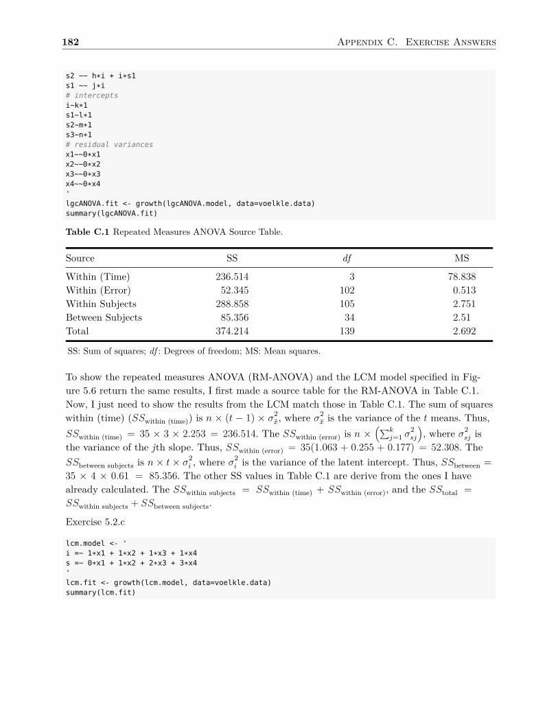
182 Appendix C. Exercise Answers
s2 ~~ h*i + i*s1s1 ~~ j*i# interceptsi~k*1s1~l*1s2~m*1s3~n*1# residual variancesx1~~0*x1x2~~0*x2x3~~0*x3x4~~0*x4'lgcANOVA.fit <- growth(lgcANOVA.model, data=voelkle.data)summary(lgcANOVA.fit)
Table C.1 Repeated Measures ANOVA Source Table.
Source SS df MS
Within (Time) 236.514 3 78.838Within (Error) 52.345 102 0.513Within Subjects 288.858 105 2.751Between Subjects 85.356 34 2.51Total 374.214 139 2.692
SS: Sum of squares; df : Degrees of freedom; MS: Mean squares.
To show the repeated measures ANOVA (RM-ANOVA) and the LCM model specified in Fig-ure 5.6 return the same results, I first made a source table for the RM-ANOVA in Table C.1.Now, I just need to show the results from the LCM match those in Table C.1. The sum of squareswithin (time) (SSwithin (time)) is n × (t − 1) × σ2
x̄, where σ2x̄ is the variance of the t means. Thus,
SSwithin (time) = 35 × 3 × 2.253 = 236.514. The SSwithin (error) is n ×(∑k
j=1 σ2sj
), where σ2
sj isthe variance of the jth slope. Thus, SSwithin (error) = 35(1.063 + 0.255 + 0.177) = 52.308. TheSSbetween subjects is n× t× σ
2i , where σ
2i is the variance of the latent intercept. Thus, SSbetween =
35 × 4 × 0.61 = 85.356. The other SS values in Table C.1 are derive from the ones I havealready calculated. The SSwithin subjects = SSwithin (time) + SSwithin (error), and the SStotal =SSwithin subjects + SSbetween subjects.
Exercise 5.2.c
lcm.model <- 'i =~ 1*x1 + 1*x2 + 1*x3 + 1*x4s =~ 0*x1 + 1*x2 + 2*x3 + 3*x4'lcm.fit <- growth(lcm.model, data=voelkle.data)summary(lcm.fit)
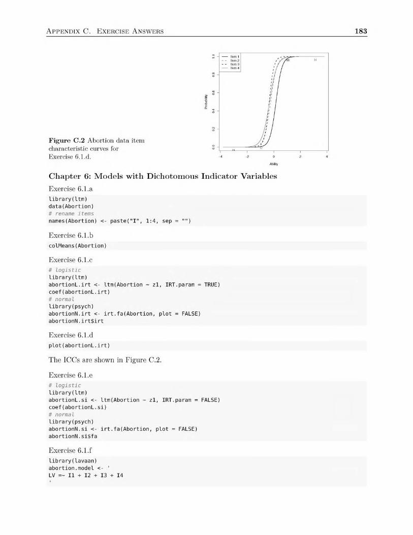
A p p e n d i x C. E x e r c i s e A n s w e r s 183
Figure C .2 Abortion data item characteristic curves forExercise 6.1.d. - 4 - 2 0 2 4
Ability
C h a p te r 6: M odels w ith D ichotom ous In d ic a to r V ariablesExercise 6.1.alibrary(ltm)data(Abortion)# rename itemsnames(Abortion) <- paste("I", 1:4, sep = "")
Exercise 6.1.bcolMeans(Abortion)
Exercise 6.1.c# logistic library(ltm)abortionL.irt <- ltm(Abortion ~ z1, IRT.param = TRUE) coef(abortionL.irt)# normal library(psych)abortionN.irt <- irt.fa(Abortion, plot = FALSE) abortionN.irt$irt
Exercise 6.1.d plot(abortionL.irt)
The ICCs are shown in Figure C.2.
Exercise 6.1.e# logistic library(ltm)abortionL.si <- ltm(Abortion ~ z1, IRT.param = FALSE) coef(abortionL.si)# normal library(psych)abortionN.si <- irt.fa(Abortion, plot = FALSE) abortionN.si$fa
Exercise 6.1.flibrary(lavaan) abortion.model <- 'LV =~ I1 + I2 + I3 + I4
I4I3Item 1 Item 2 Item 3 Item 4
184 Appendix C. Exercise Answers
abortion.fit <- cfa(abortion.model, data=Abortion, std.lv=TRUE,ordered=paste("I",seq(1:4), sep=""))summary(abortion.fit)
Exercise 6.2.agss.data <- read.table("gss2000.dat", header = TRUE)
Exercise 6.2.b & Exercise 6.2.cgssConversion.model<-'# loadingsTheta =~ l1*word.a + l2*word.b + l3*word.c + l4*word.d + l5*word.e + l6*word.f + l7*word.g +l8*word.h + l9*word.i + l10*word.j# thresholdsword.a | th1*t1word.b | th2*t1word.c | th3*t1word.d | th4*t1word.e | th5*t1word.f | th6*t1word.g | th7*t1word.h | th8*t1word.i | th9*t1word.j | th10*t1# convert loadings to slopes (logistic scale)alphaa.L := (l1)/sqrt(1-l1^2)*1.7alphab.L := (l2)/sqrt(1-l2^2)*1.7alphac.L := (l3)/sqrt(1-l3^2)*1.7alphad.L := (l4)/sqrt(1-l4^2)*1.7alphae.L := (l5)/sqrt(1-l5^2)*1.7alphaf.L := (l6)/sqrt(1-l6^2)*1.7alphag.L := (l7)/sqrt(1-l7^2)*1.7alphah.L := (l8)/sqrt(1-l8^2)*1.7alphai.L := (l9)/sqrt(1-l9^2)*1.7alphaj.L := (l10)/sqrt(1-l10^2)*1.7# convert thresholds to locations (logistic scale)loca.L := th1/l1locb.L := th2/l2locc.L := th3/l3locd.L := th4/l4loce.L := th5/l5locf.L := th6/l6locg.L := th7/l7loch.L := th8/l8loci.L := th9/l9locj.L := th10/l10'
gssConversion.fit <- cfa(gssConversion.model, data = gss.data, std.lv = TRUE,ordered = paste("word.",letters[1:10], sep=""))summary(gssConversion.fit)
The first item, word.a, is the easiest and the last item, word.j, is the most difficult.
Exercise 6.2.dlibrary(ltm)gss.IRT <- ltm(gss.data ~ z1, IRT.param = TRUE)coef(gss.IRT)
Appendix C. Exercise Answers 185
Chapter 7: Models with Missing DataExercise 7.1.amcar.data <- read.table("mcar.dat", sep = ",", header = TRUE)mar.data <- read.table("mar.dat", sep = ",", header = TRUE)nmar.data <- read.table("nmar.dat", sep = ",", header = TRUE)
Exercise 7.1.blibrary(BaylorEdPsych)library(MissMech)
LittleMCAR(mcar.data)TestMCARNormality(mcar.data)
LittleMCAR(mar.data)TestMCARNormality(mar.data)
LittleMCAR(nmar.data)TestMCARNormality(nmar.data)
Exercise 7.1.ccomplete.model <- 'read =~ a*z1 + b*z2 + c*z3read ~ g*x1
z1~~d*z1z2~~e*z2z3~~f*z3read~~h*read'
mcarListwise.fit <- sem(complete.model, data=mcar.data)marListwise.fit <- sem(complete.model, data=mar.data)marListwise.fit <- sem(complete.model, data=nmar.data)
Exercise 7.1.dmcarFIML.fit <- sem(complete.model, data=mcar.data, missing='fiml')marFIML.fit <- sem(complete.model, data=mar.data, missing='fiml')marFIML.fit <- sem(complete.model, data=nmar.data, missing='fiml')
Exercise 7.1.elibrary(semTools)mcarFIMLAux.fit <- auxiliary(complete.model, aux="x2", data=mcar.data, fun="sem")marFIMLAux.fit <- auxiliary(complete.model, aux="x2", data=mar.data, fun="sem")marFIMLAux.fit <- auxiliary(complete.model, aux="x2", data=nmar.data, fun="sem")
Exercise 7.1.flibrary(semTools)mcarMI.fit <- runMI(complete.model, data=mcar.data, m=20, miPackage="mice", fun="sem")marMI.fit <- runMI(complete.model, data=mar.data, m=20, miPackage="mice", fun="sem")nmarMI.fit <- runMI(complete.model, data=nmar.data, m=20, miPackage="mice", fun="sem")
Exercise 7.2.aeating.data <- read.table("eatingattitudes.dat")# remove first variableeating.data$id <- NULL
186 Appendix C. Exercise Answers
Exercise 7.2.blibrary(mice)md.pattern(eating.data)
Exercise 7.2.clibrary(BaylorEdPsych)library(MissMech)
LittleMCAR(eating.data)TestMCARNormality(eating.data)
The missing values do not appear to be MCAR.
Exercise 7.2.dlibrary(lavaan)eating.model <- 'drive =~ eat1 + eat2 + eat10 + eat11 + eat12 + eat14 + eat24foodpre =~ eat3 + eat18 + eat21'
eatingListwise.fit <- cfa(eating.model, data=eating.data)summary(eatingListwise.fit, standardized=TRUE)
There are 267 observations using listwise deletion.
Exercise 7.2.eeatingFIML.fit <- cfa(eating.model, data = eating.data, missing = "fiml")summary(eatingFIML.fit, standardized = TRUE)
Exercise 7.2.flibrary(semTools)eatingFIMLAux.fit <- auxiliary(eating.model, aux = c("bmi", "wsb", "anx"), data = eating.data,
fun = "sem")summary(eatingFIMLAux.fit, standardized = TRUE)
Exercise 7.2.glibrary(semTools)# make the eating items categorical for the imputation processitems <- paste("eat", c(1, 2, 10, 11, 12, 14, 24, 3, 18, 21), sep = "")eating.data[, items] <- lapply(eating.data[, items], as.factor)
# create imputed dataset via Amelialibrary(Amelia)eating.amelia <- amelia(eating.data, m = 20, ords = paste("eat", c(1, 2, 10, 11, 12, 14, 24,
3, 18, 21), sep = ""))
eatAmelia.fit <- runMI(eating.model, data = eating.amelia$imputations, fun = "cfa")summary(eatAmelia.fit)
# create imputed dataset via micelibrary(mice)eating.mice <- mice(eating.data, m = 20, meth = c(rep("polyreg", 10), rep("pmm", 3)))
# place all the imputed mice datasets into a single listeating.mice.data <- NULLfor (i in 1:20) {
eating.mice.data[[i]] <- complete(x = eating.mice, action = i, include = FALSE)
Appendix C. Exercise Answers 187
}
eatMice.fit <- runMI(eating.model, data = eating.mice.data, fun = "cfa")summary(eatMice.fit, standardized = TRUE)
Chapter 8: Sample Size PlanningExercise 8.1.a
If g = 0.40, then Y ’s variance is 0.40× 0.25× 0.40 + 1× 0.80× 1 = 0.84. That makes
d = 0.15√0.84
= 0.436
Exercise 8.1.b# data generating modelread.pop.model <- 'read =~ 1*z1 + 0.90*z2 + 0.60*z3# regressionread ~ g*x1 + 0.40*x1# means and variancesx1~0.5*1z1~0*1z2~0*1z3~0*1# variancesx1~~0.25*x1z1~~0.80*z1z2~~0.80*z2z3~~0.40*z3read~~0.80*read'# analysis modelread.model <- 'read =~ z1 + z2 + z3read ~ g*x1'# population momentsread.fit<-sem(read.pop.model, do.fit=FALSE, fixed.x=FALSE)summary(read.fit,rsquare=TRUE)fitted(read.fit)# monte carlo simulationread.n <- sim(model=read.model, n =rep(seq(100,300,25), 500), generate=read.pop.model,lavaanfun = "sem", multicore=TRUE)# power curveplotPower(read.n, alpha=0.05, powerParam=c("g"))abline(h=.8, lwd=2, lty=2)
The power curve is shown in Figure C.3.
Exercise 8.1.cAccording to the power curve, there should be enough power when n ≈ 220.
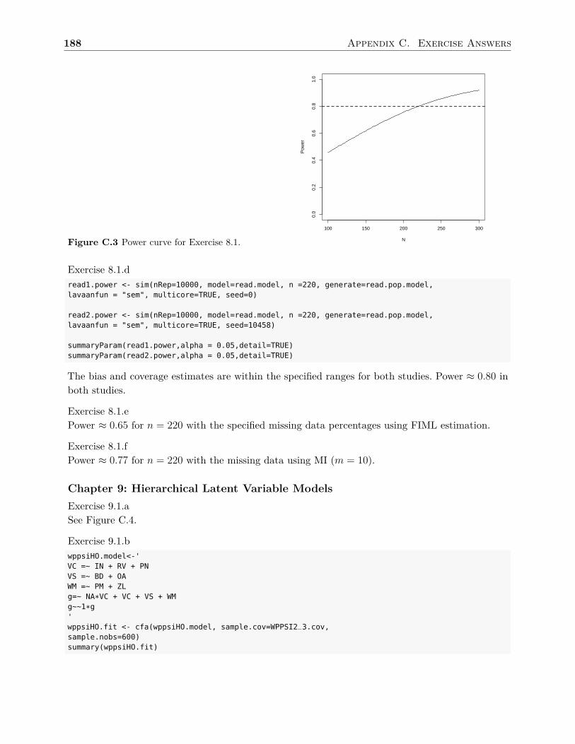
188 Appendix C. Exercise Answers
Figure C.3 Power curve for Exercise 8.1.100 150 200 250 300
0.0
0.2
0.4
0.6
0.8
1.0
N
Pow
er
Exercise 8.1.dread1.power <- sim(nRep=10000, model=read.model, n =220, generate=read.pop.model,lavaanfun = "sem", multicore=TRUE, seed=0)
read2.power <- sim(nRep=10000, model=read.model, n =220, generate=read.pop.model,lavaanfun = "sem", multicore=TRUE, seed=10458)
summaryParam(read1.power,alpha = 0.05,detail=TRUE)summaryParam(read2.power,alpha = 0.05,detail=TRUE)
The bias and coverage estimates are within the specified ranges for both studies. Power ≈ 0.80 inboth studies.
Exercise 8.1.ePower ≈ 0.65 for n = 220 with the specified missing data percentages using FIML estimation.
Exercise 8.1.fPower ≈ 0.77 for n = 220 with the missing data using MI (m = 10).
Chapter 9: Hierarchical Latent Variable ModelsExercise 9.1.aSee Figure C.4.
Exercise 9.1.bwppsiHO.model<-'VC =~ IN + RV + PNVS =~ BD + OAWM =~ PM + ZLg=~ NA*VC + VC + VS + WMg~~1*g'wppsiHO.fit <- cfa(wppsiHO.model, sample.cov=WPPSI2_3.cov,sample.nobs=600)summary(wppsiHO.fit)
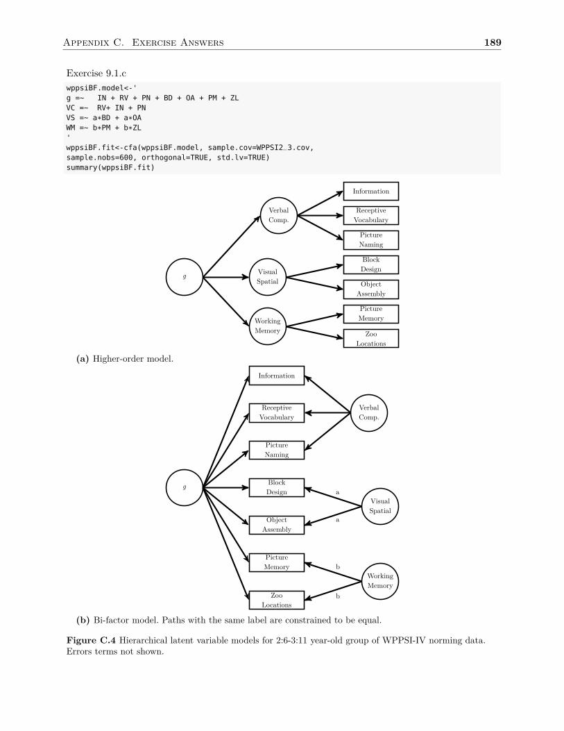
Appendix C. Exercise Answers 189
Exercise 9.1.cwppsiBF.model<-'g =~ IN + RV + PN + BD + OA + PM + ZLVC =~ RV+ IN + PNVS =~ a*BD + a*OAWM =~ b*PM + b*ZL'wppsiBF.fit<-cfa(wppsiBF.model, sample.cov=WPPSI2_3.cov,sample.nobs=600, orthogonal=TRUE, std.lv=TRUE)summary(wppsiBF.fit)
Information
ReceptiveVocabulary
PictureNaming
BlockDesign
ObjectAssembly
PictureMemory
ZooLocations
VerbalComp.
VisualSpatial
WorkingMemory
g
(a) Higher-order model.
Information
ReceptiveVocabulary
PictureNaming
BlockDesign
ObjectAssembly
PictureMemory
ZooLocations
g
VerbalComp.
VisualSpatial
WorkingMemory
a
a
b
b
(b) Bi-factor model. Paths with the same label are constrained to be equal.
Figure C.4 Hierarchical latent variable models for 2:6-3:11 year-old group of WPPSI-IV norming data.Errors terms not shown.

Glossary
Italicized words indicate other terms in glossary.
Alternative fit index (AFI) Measure of how a latent variable model fits a given dataset that isan alternative to the traditional χ2-distributed statistic. Sometimes called practical fitindex.
Auxiliary variable (AV) A variable that is not of interest in answering a research question, butis included in the model because it is either a potential cause or correlate of missingnessin the variables of interest.
Behavior genetics (BG) Academic field that examines the genetic and/or environmental influ-ences on physical or behavioral traits (i.e., a phenotype) by using genetically informativeresearch designs.
Bi-factor latent variable model A type of hierarchical latent variable model comprised offirst-order latent variables. The general latent variable influences all the manifest vari-ables, while the domain-specific latent variables only influence a subset of the manifestvariables. Sometimes called a nested-factors or direct hierarchical model.
Bias In a Monte Carlo Study, the difference between the actual parameter value and the averageof all the estimated values. See also relative bias.
Communality The proportion of an indicator variable’s variance that is due to the latent vari-ables in the model. It is calculated as the sum of the squared standardized loadings forall latent variables that influence a given variable.
Conditional parameterization Item factor analysis parameterization that constrains the un-derlying variables’ error variances to be 1.0, and typically constrains the thresholds totheir values when estimated using the marginal parameterization. The variance of theunderlying variables are calculated from the loadings and the latent variable’s variance.Sometimes called the theta or unstandardized parameterization.
Configural invariance First step in assessing measurement invariance. It requires the indicatorvariables form the same latent variable structure (i.e., number of LVs, number of indica-tor variables, pattern of constrained and estimated parameters) in all groups.
Confirmatory factor analysis (CFA) A statistical technique for data reduction that specifiesthe number, meaning, and associations of the latent variables, as well as the pattern ofthe estimated factor loadings, before analyzing the data. See latent variable model.
Coverage In a Monte Carlo Study, the proportion of confidence intervals, across all the simu-lated datasets, that contain the actual parameter value. It is a measure of standard erroraccuracy.
Degrees of freedom (df ) In a latent variable model, it is the difference between the numberof non-redundant pieces of information in the data and the number of parameters toestimate. Will only be > 0 for overidentified models.
Domain-specific latent variable In a bi-factor latent variable model, they are the latent vari-ables that only influence a portion of the manifest variables.
190
Glossary 191
Empirical underidentification Situation when a latent variable model is only identified if oneof its parameters (usually a latent correlation or loading) is not equal to 0.0 or 1.0. Seeidentification of latent variable.
Endogenous variable A variable that has at least one direct cause within a specific model. Inregression, it is sometimes called an outcome, criterion, or downstream variable, whilewith an experimental design it is called dependent variable.
Error The discrepancy between an observations’s actual value on a variable and the value pre-dicted by the other variables in the model. The discrepancies’ variability represents theamount of variance in an endogenous variable not explained by the other variables in themodel. Sometimes called a residual or disturbance..
Exogenous variable A variable that has no direct cause within a specific model. In regression,it is sometimes called a predictor, source, or upstream variable, while in an experimentaldesign it is called an independent variable.
Exploratory factor analysis (EFA) A statistical method for reducing data whereby factors(i.e. latent variables) are extracted from a dataset without specifying the number andpattern of factor loadings between the manifest variables and the factors.
Factor A latent variable.Factor loading The relationship between an indicator variable and a latent variable. With re-
flective latent variables, they are interpreted as regression coefficients (i.e, how much doesthe indicator variable increase as the latent variable increases a single unit). The largerthe absolute value of the loading, the more relevant the indicator variable is in definingthe latent variable.
First-order latent variable (FOLV) Latent variables with manifest indicator variables. Seealso higher-order latent variable model and bi-factor latent variable model.
Formative latent variable A latent variable that is the weighted sum of the indicator variables.Unlike a reflective latent variable, a formative latent variable model posits that the latentvariable is the result of the indicator variables. Sometimes called an emergent factor.
Full information maximum likelihood (FIML) Type of maximum likelihood parameter es-timation technique that finds the most likely parameter estimates for each observation,with the final model estimates being the ones that are the most likely across all observa-tions. One modern method for handling missing data.
Higher-order latent variable model A type of hierarchical latent variable model where first-order latent variables serve as indicator variables to form second-order latent variables.Sometimes called an indirect hierarchical or second-order latent variable model.
Identification of latent variable Determination of whether a model’s parameters can be uniquelydetermined from the amount of non-redundant information in the data (i.e., covariances,variances, and, when applicable, means).
Indicator variable In reflective latent variable models, indicator variables are manifest variablesthat are directly influenced by one or more latent variables and an error term.
Indirect effect The influence of one variable on a second variable through a third (or fourth, orfifth, . . . ) variable. The indirect variables are mediating variables.
192 Glossary
Item characteristic curve Graphical representation of an item response theory model thatshows the probability of endorsing a given response to an item (e.g., answering correctly)as a function of the latent variable.
Item discrimination In item response theory models, it is the measure of both how well anitem measures the latent variable and how well an item differentiates between examineeshaving abilities below and above the item location.
Item factor analysis (IFA) Latent variable model with categorical indicator variables. They canbe parameterized to give results equivalent to models based on item response theory.
Item location In an item response theory model, it is a description of where the item best func-tions along the latent variable’s scale. Sometimes called item difficulty.
Item response theory (IRT) Broad class of latent variable models designed to describe theprobability of a response to a categorical indicator variable, conditional on the level ofthe latent variable.
Just-identified model A model with the same number of parameters to estimate as there isnon-redundant information in the data. Thus, the degrees of freedom are always zero.Sometimes called a saturated model. See identification of latent variable.
Latent curve model (LCM) Latent variable model used to model change over time for oneor more variables measured on the same individuals. Sometimes called a latent growthcurve or latent trajectory model.
Latent variable (LV) A variable for which values cannot be directly observed. Its measurementhas to be inferred from values on one or more manifest variables. Sometimes called afactor or a construct.
Latent variable model (LVM) A statistical model that relates a set of manifest variables toone of more latent variables. Sometimes called a measurement model, factor analysis, orconfirmatory/exploratory factor analysis.
Manifest variable (MV) A variable that can be directly observed and measured.Marginal parameterization Item factor analysis parameterization that standardizes the marginal
(unconditional) distribution of the underlying variables, which then makes the scaling fac-tor equal 1.0. The underlying variables’ error variances are calculated from the loadingsand the latent variable’s variance. Sometimes called the delta or standardized parameteri-zation.
Mean and covariance structure (MACS) Extension of typical latent variable model wherebymean-level information is analyzed (structured) in addition to the covariances.
Measurement invariance When the relationship between the indicator variables and the latentvariables does not differ among two or more groups.
Missing at random (MAR) When missing values on a given variable are unrelated to the vari-able itself, but are related to other variables. For the parameter estimates to be unbiased,the variables related to the missingness must be included in the model.
Missing completely at random (MCAR) When missing values on a given variable are unre-lated to both that variable and any other variable.
Missing data pattern Configuration of observed and missing values in a dataset.Monte Carlo Study (MC) An experiment in which variable or model properties are investi-
gated by using purposefully simulated data.
Glossary 193
Multiple imputation (MI) Method for handling missing data that creates multiple datasets,each of which contain different plausible estimates of the missing values.
Multiple indicators multiple independent causes model (MIMIC) Latent variable modelwith at least one exogenous manifest variable (the independent causal indicator[s]) pre-dicting an endogenous latent variable.
Nested model A model that estimates a subset of another model’s parameters, and thus hasfewer degrees of freedom.
Not missing at random (NMAR) When missing values on a given variable are related to thevariable itself, even after including all possible covariates in the model. Sometimes callednon-ignorable missingness or missing not at random.
Overidentified model A model with fewer parameters to estimate than non-redundant informa-tion in the data. See identification of latent variable.
Partial invariance Model where a measurement invariance constraint is not warranted for onlya few of the parameter estimates within an invariance level, but is warranted for all theothers.
Path coefficient A measure of the direct effect of one variable on another variable. Usuallyassumed to be standardized (i.e., variables transformed to Z scores) unless otherwisestated. Sometimes called regression coefficients, especially if latent variables are not in-cluded in the path model.
Path model An diagram of variable relationships that uses geometric figures to represent vari-able types, and arrows to represent variable relationships. Single-headed arrows showdirect relationships, whereas double-headed arrows indicate a non-directional (i.e., covari-ance) relationships. Sometimes called path diagram or path figure.
Pattern coefficient See factor loading.Power The frequency of concluding the data, taken from multiple samples of the same popula-
tion, indicate a variable has an effect when there is one in the population. In a MonteCarlo Study, it is the proportion of the simulated datasets for which the null hypothesisis rejected for a parameter estimate at a given type 1 error rate (i.e., how often p-value< α).
Random effects A model parameter that can vary across observations, which allows it to haveunexplained (i.e, error) variance.
Reflective latent variable Latent variable model where the indicator variables are dependenton, or the results of, the latent variable. Sometimes called an effect indicator model.
Relative bias A method to make bias estimates from a Monte Carlo Study comparable by divid-ing the bias estimate by the known population value. The resulting values are in propor-tions.
Robust estimator Parameter estimators whose values are less influenced by assumption viola-tions than the traditional maximum likelihood estimator.
Second-order latent variable (SOLV) In a higher-order latent variable model, they are latentvariables formed by using other latent variables as indicator variables.
Specific factor In a higher-order latent variable model, the part of a first-order latent variablenot explained by the second-order latent variable.

194 Glossary
Strict invariance Fourth step in assessing measurement invariance, although some consider itan optional step. It requires that indicator variables’ error variances are the same acrossgroups.
Strong invariance Third step in assessing measurement invariance. It requires that indicatorvariables’ intercepts are the same across groups. Sometimes called scalar invariance.
Structural equation model (SEM) A model that consists of manifest variables and latent vari-ables, as well as a structural model (path model) specifying their relationships. Sometimescalled a simultaneous equation model, linear structural relationship model, or covariancestructure analysis.
Structural invariance Assess if latent variances, covariance, or means are the same acrossgroups. Can only be assessed with models that at least have strong invariance.
Structure coefficient Correlation of an indicator variable with a latent variable. Only whenthe latent variables are uncorrelated, or there is one latent variable, do the structurecoefficients and pattern coefficients (factor loadings) have the same values.
Tetrachoric correlation Correlation between two dichotomous variables, each of which arecoarse measures of a normally-distributed underlying variable and, together, have abivariate-normal distribution. The resulting value approximates what the Pearson cor-relation would have been between the variables if they were measures on a continuousscale.
Time-invariant covariate Covariate for a latent curve model whose values are stable over allthe data collection time periods.
Time-varying covariate Covariate for a latent curve model whose values can vary across thedata collection time periods.
Tracing rules Standard rules for reading paths in a path model that yield the expected vari-ances and covariances among the model’s variables. Sometimes called Wright’s rules,after Sewall Wright.
Underidentified model A model with more parameters to estimate than non-redundant infor-mation in the data. See identification of latent variable.
Underlying variable Continuous latent variable, often assumed to follow normal distribution,that underlies a dichotomous variable in item factor analysis models. Categorical indica-tor variables (i.e,. items) are course measurements of the underlying variable.
Uniqueness The proportion of an indicator variable’s variance that is not explained by the la-tent variables in the model. It is calculated as one minus the communality.
Weak invariance Second step in assessing measurement invariance. It requires that indicatorvariables’ loadings are the same across groups. Sometimes called pattern or metric invari-ance.

Author IndexAdler, M. A., 130Aiken, L. S., 89, 92American Psychological Association Science
Directorate Task Force on StatisticalInference, 118, 130
Asendorpf, J. B., 33, 36Asparouhov, T., 130
Bagozzi, R. P., 55Baker, F. B., 113Barrett, P., 133, 144Bartholomew, D., 111, 113Bates, T., 169, 170Bauer, D. J., 113Bauman, S., 128, 130Baumgartner, H., 78Beauducel, A., 113Beaujean, A. A., 20, 31, 37, 43, 52, 53, 55,
62, 65, 75, 78, 111, 113, 148, 151,152
Bentler, P. M., 156, 166Bock, R. D., 94, 113Bohr, Y., 129, 130Boker, S. M., 36, 169, 170Bolger, N., 55Bollen, K. A., 38, 55, 80, 81, 84, 88, 92Boomsma, A., 51, 55, 75, 78Borenstein, M., 143, 144Braddy, P. W., 61, 78Brick, T., 169, 170Briggs, N. E., 92Brosseau-Liard, P. É., 113Brown, T. A., 55Brunner, M., 152Byrnes, J. E., 169, 170
Camilli, G., 102, 113Card, N. A., 55, 77, 78, 128, 130Carlson, G., 62, 65, 78Chen, F. F., 152
Chou, C.-P., 55Coalson, D. L., 151, 152Cohen, J., 89, 92Cohen, P., 89, 92Conner, M., 33, 36Cotter, R. A., 94, 113Crawley, M., 20Curran, P. J., 80, 81, 84, 88, 92, 113
De Fruyt, F., 33, 36De Houwer, J., 33, 36DeFries, J. C., 71, 78DeMaris, A., 130Denissen, J. J. A., 33, 36DiStefano, C., 113
Edwards, J. R., 55Edwards, M. C., 113Embretson, S. E., 113Enders, C. K., 129, 130Estabrook, R., 169, 170
Fiedler, K., 33, 36Fiedler, S., 33, 36Field, A., 20Field, Z., 20Finch, J. F., 113Finney, S. J., 113Flora, D. B., 113Forero, C. G., 110, 113Fox, J., 167, 169, 170Freeman, M. J., 62, 65, 78Funder, D. C., 33, 36
Galbraith, J., 111, 113Garfinkel, P. E., 129, 130Garner, D. M., 129, 130Graham, J. M., 54, 55Graham, J. W., 114, 130Groothuis-Oudshoorn, K., 120, 130Guttman, L., 101, 113
195

196 Author Index
Hallquist, M., 167, 170Herzberg, P. Y., 113Ho, M.-H. R., 51, 55Horn, J. L., 56, 78Hoyle, R. H., 51, 55, 75, 78Huh, J., 55Hunter, A. M., 130
Jalal, S., 123, 128, 130Jamshidian, M., 123, 128, 130Janke, M. C., 52, 53, 55Jansen, C., 123, 128, 130Johnson, E. C., 61, 78
Kamata, A., 113Kashy, D., 55Keith, T. Z., 34Kelley, K., 131, 133, 144Kenny, D. A., 55Kenny, S., 169, 170Kim, S.-H., 113Kliegl, R., 33, 36
Lance, C. E., 60, 78Ledford, E. C., 78Leuchter, A. F., 130Li, S.-C., 152Lieberman, M., 94, 113Little, R. J. A., 114, 116, 123, 128, 130Little, T. D., 55, 77, 78Loehlin, J. C., 55Lottes, I. L., 130
MacCallum, R. C., 92MacKinnon, D. P., 34Maes, H. H. M., 72, 78, 169, 170Matloff, N., 20Maxwell, S. E., 131, 133, 144Maydeu-Olivares, A., 110, 113McArdle, J. J., 36, 56, 78, 130McClearn, G. E., 71, 78McDonald, R. P., 51, 55, 165, 166McGuffin, P., 71, 78McLeod, L. D., 152Meade, A. W., 61, 78
Mehta, P., 169, 170Miles, J., 20Miller, P., 134, 144Millsap, R. E., 78Moustaki, I., 111, 113Muthén, B. O., 92, 130, 133–135, 137, 140,
144, 167, 170Muthén, L. K., 133–135, 137, 140, 144, 167,
170
Nagy, G., 152Neale, M. C., 72, 78, 169, 170Nicol, A. A. M., 34, 52, 55Nosek, B. A., 33, 36
Olmsted, M. P., 129, 130
Page, E. B., 34Panter, A. T., 51, 55, 75, 78Parkin, J., 43, 55, 148, 152Perugini, M., 33, 36Pexman, P. M., 34, 52, 55Plomin, R., 71, 78Pornprasertmanit, S., 134, 144Preacher, K. J., 92
R Development Core Team, 20Raiford, S. E., 151, 152Reese, L. M., 94, 113Reise, S. P., 113Revelle, W., 20Rhemtulla, M., 113Rizopoulos, D., 113Roberts, B. W., 33, 36Rosseel, Y., 36Rubin, D. B., 114, 130Rutter, M. , 78
Satorra, A., 156, 166Savalei, V., 113Schafer, J. L., 130Schlomer, G. L., 128, 130Schmiedek, F., 152Schmitt, M., 33, 36Schoemann, A., 134, 144

Author Index 197
Sheng, Y., 75, 78, 111, 113Slegers, D. W., 55, 77, 78Sousa, K. H., 152Spiegel, M., 169, 170Spies, J., 169, 170Steele, F., 111, 113Steenkamp, J.-B. E. M., 78
Thissen, D., 152
Umstattd-Meyer, M. R., 52, 53, 55
van Aken, M. A. G., 33, 36van Buuren, S., 120, 130Vandenberg, R. J., 60, 78Voelkle, M, C., 91, 92
Watkins, M. W., 151, 152
Weber, H., 33, 36Wechsler, D., 38, 55, 62, 65, 78, 148, 151,
152West, S. G., 89, 92, 113, 152Wicherts, J. M., 33, 36Wichman, A. L., 92Wilde, M., 169, 170Wiley, J., 167, 170Wilhelm, O., 152Wilkinson, L., 118, 130Wirth, R. J., 113Wolfle, L. M., 36Wright, S., 23, 36, 194
Youngstrom, E., 62, 65, 78Yuan, K.-H., 156, 166Yung, Y.-F., 152

Subject Index
Bold page numbers indicate page number for glossary entry.
Auxiliary Variable (AV), 121, 125, 190
Behavior Genetics, 71–74, 190Bi-Factor Model, see Latent Variable ModelBias, see Monte Carlo Study
Categorical Variable, see Indicator VariableConditional Parameterization, see Item Fac-
tor AnalysisConfirmatory Factor Analysis, see Latent
Variable ModelConstruct, see Latent VariableCorrelation, 14
Matrix, see CovarianceModel-Implied, 46Pearson, 14Residual, 46Spearman, 14Tetrachoric, 96, 105, 194
Covariance, 14MatrixData Entry, 7, 29
Model-Implied, 46Residual, 46
Coverage, see Monte Carlo Study, 133
Degrees of Freedom, 40, 45, 61, 154, 190Dichotomous Variable, see Indicator VariableDifficulty, see Item LocationDiscrimination, see Item Response TheoryDisturbance, see ErrorDomain-Specific Latent Variable, see Latent
Variable
Empirical Underidentification, see Identifica-tion of Latent Variable
Endogenous Variable, see Variable, 57Error, 22, 24, 26, 38, 40, 42, 50, 59, 73, 83,
86, 99, 100, 145, 191
Exogenous Variable, see Variable, 57Exploratory Factor Analysis, 37, 121, 191
Factor, see Latent VariableFactor Analysis, see Latent Variable Model,
190Factor Loading, 38, 39, 48, 191FIML, see Full Information Maximum Likeli-
hoodFirst-Order Latent Variable, 145, see Latent
VariableFit Indexes, 153–166
Alternative Fit Indexes, 154, 158–165,190
χ2, 153–158Robust, 156–158
Residuals, 165–166Full Information Maximum Likelihood
(FIML), 119, 124, 191
Heritability, 71Higher-Order Model, see Latent Variable
ModelHomogeneity of Latent Variable Variances,
see Invariance
Identification of Latent Variable Model, 39–42, 191
Empirical Underidentification, 42, 150,191
Hierarchical Model, 147Just-Identified, 39, 192Latent Variable Scale, 41, 47–48Means and Intercepts, 58Number of Indicator Variables, 40–41Overidentified, 39, 193Underidentified, 39, 194
Imputation, see Missing Data
198
Subject Index 199
Indicator Variable, 38, 40–41, 191Categorical/Dichotomous, 93
Indirect Effect, 30–32, 191Invariance, 56, 58, 62–70, 192
Configural, 58, 190Evaluation, 61Latent Variable Covariances, 59Latent Variable Means, 59Latent Variable Variances, 59Partial, 60, 68, 193Strict, 59, 194Strong, 59, 194Structural, 60, 194Weak, 59, 194
Inverse Logit, 140Item Characteristic Curve, 100, 106, 192Item Factor Analysis, 96–100, 104, 192
Conditional Parameterization, 100, 190Conversion Formulae, 104Delta Parameterization, see Marginal
ParameterizationMarginal Parameterization, 99, 192Theta Parameterization, see Conditional
ParameterizationThreshold, 96, 97Underlying Variable, 96–103, 194
Item Response Theory, 100–104, 192Conversion Formulae, 104Cumulative Logistic Distribution Con-
stant (D), 102, 105Item Discrimination, 102, 192Item Location, 101, 102, 192Logistic, 102Normal Ogive, 101
Latent Curve Model, 79–88, 137–142, 192Fixing Loadings, 79Interaction, 87Non-Linear Change, 88Piecewise Linear Change, 88Time-Invariant Covariate, 84, 85, 194Time-Variant Covariate, 84, 85Time-Varying Covariate, 194
Latent Variable, 23, 192
Domain-Specific, 147, 190First-Order, 191Formative, 38, 54, 191Identification, see Identification of La-
tent Variable ModelReflective, 38, 193Scale, 41Effects-Coding, 41, 48, 58Marker Variable, 41, 44, 58Standardized, 41, 47, 58
Second-Order, 193Latent Variable Model, 37–39, 192
Bi-Factor, 146–148, 190Communality, 39, 190Higher-Order, 145–147, 191Identification, see Identification of La-
tent Variable ModelMeans and Intercepts, 56–58Single-Indicator, 40, 42Uniqueness, 39, 194
LATEX, 33Listwise Deletion, see Missing Data
MACS, see Mean and Covariance StructureManifest Variable, see VariableMarginal Parameterization, see Item Factor
AnalysisMean and Covariance Structure (MACS), 56,
192Measurement Invariance, see Invariance, see
InvarianceMI, see Multiple ImputationMIMIC, see Multiple Indicators Multiple
Independent CausesMissing Data
Pattern, 114, 192Auxiliary Variable, see Auxiliary Vari-
ableFull Information Maximum Likelihood,
see Full Information Maximum Like-lihood
Imputation, 118in R, 11Listwise Deletion, 12, 118
200 Subject Index
Missing at Random (MAR), 116, 192Missing Completely at Random
(MCAR), 114, 192Multiple Imputation, see Multiple Impu-
tationNot Missing at Random (NMAR), 117,
193Pairwise Deletion, 118Planned Missing Design, 115
Model Modification, 47Expected Parameter Change, 47Modification Index, 47
Monte Carlo Study, 133–137, 192Bias, 190Parameter Estimate, 133Relative Parameter Estimate, 133
Coverage, 190Relative Bias, 193Standard Error Bias, 133
Multiple Imputation (MI), 119–121, 125,193
Chained Equations, 120Multiple Indicators Multiple Independent
Causes (MIMIC), 85, 86, 193
Nested Model, 155, 193Noncentrality Parameter, 161
Ogive, 101
Pairwise Deletion, see Missing DataParameter Constraint, 48, 61–62, 70–71
Group Equality Constraint, 61–62Labels, 70–71Specific Value, 71
Parameter Estimation, 98, 103Full Information, 103Least Squares, 98, 157Limited Information, 98Robust Estimator, 156, 157, 193Weighted Least Squares, 98Robust (WLSMV), 98, 108, 110, 157
Partial Invariance, see InvariancePath Analysis, 23–30Path Coefficient, 26–27, 193
Standardized, 26Unstandardized, 26
Path Model, 21–23, 193Symbols, 21
Pattern Coefficient, see Factor LoadingPower, 131, 193
RComment, 3Concatenate, 3Correlation, 14Covariance, 14DataCategorical, 12Factor, 12Import from External Source, 6Import from Other Programs, 6Input, 5Manipulation, 10Packages, 7Simulation, see SimulationSort, 11Subset, 10, 11Summarizing, 12
Data Frame, 6Descriptive Statistics, 12Factors, 12Function, 2–4Actual Argument, 4Formal Argument, 4Writing, 4
Help, 3Installing, 2Lists, 64, 73Logical Operators, 48Missing Data, 11NA, 6, 11, 48, 129
Packages, 4Simulation, 8Table, 13Frequency, 13Relative Frequency, 13
R2, 24, 26, 29, 39, 86
Random Effects, 80, 193
Subject Index 201
Relative Bias, see Monte Carlo StudyResidual, see Error
Sample Size Planning, 131–142Missing Data, 140–142
Second-Order Latent Variable, 145, see La-tent Variable
Specific Factor, 145, 193Standardized Coefficient, see Path Coeffi-
cientStructural Equation Model, 37, 50, 194Structure Coefficient, 39, 48, 194
t Test, 16Tetrachoric Correlation, see CorrelationThreshold, see Item Factor AnalysisTracing Rules, 23–26, 45, 46, 48, 194
Means and Intercepts, 57–58
Unstandardized Coefficient, see Path Coeffi-cient
VariableEndogenous, 21, 191Exogenous, 21, 191Latent, see Latent VariableManifest, 23, 38, 192Standardized, 14, 44
Wald Statistic, 16Wright’s Rules, see Tracing Rules
Z Score, 14Z Test, 16
R Function Index?, see help()
[[]], 66$, 8
abline(), 136anova(), 155attach(), 9auxiliary(), 125
bartlett.test(), 17
c(), 3, 5, 71cat(), 168cfa(), 28, 32, 44coef(), 106colnames(), 7, 29, 31sem(), 31Concatenate, see c()
cor(), 14cor2cov(), 43cov(), 14cov2cor(), 46cut(), 13
data(), 7cbind(), 19data.frame(), 19des(), 134describe(), 12detach(), 9
example(), 3extractModelParameters(), 168extractModelSummaries(), 168
factor(), 12file.choose(), 6findPower(), 137, 140fitMeasures(), 64fitMeasures(), 46, 153fitted(), 46, 135function(), 4
getPower(), 137growth(), 80
head(), 9help(), 3help.start(), 4
install.packages(), 5irt.fa(), 106
lavaan(), 28lavaan Model Syntax
Constant (~1), 28Constrain Parameter (>, <, ==), 48, 71Covary (~~), 28Define Formative Latent Variable (<~),
28Define Non-Model Parameter (:=), 28,
31, 108Define Reflective Latent Variable (=~),
28Define Reflective Latent Variable (~=),
44fixed.x, 125, 138Group Equality Constraint
(group.equal), 61Group Equality Constraint Release
(group.partial), 62, 67Include Means (meanstructure or
sample.mean), 64Label Parameter (*), 28, 71, 134Free Loading, 48
missing, 124ordered, 107orthogonal, 150Regress Onto (~), 28Standardize All Latent Variables
(std.lv), 48, 108, 150Threshold (|), 28, 107Use Only Starting/Fixed Values
(do.fit=FALSE), 135, 138
202

R Function Index 203
lavExport(), 169lavTables(), 166leveneTest(), 17library(), 5list(), 64, 73LittleMCAR(), 123lm(), 9lm(), 19Logical Operators, 48lower2full(), 7, 29, 31, 42ltm(), 105
md.pattern(), 123mean(), 4miss(), 140modificationIndices(), 47modindices(), 67mplus2lavaan(), 169
na.omit(), 12, 16
order(), 11, 67
parameterEstimates(), 33, 44, 52plot(), 106plotLogitMiss(), 141plotPower(), 136pnorm(), 96pwr.t.test(), 132
read.csv(), 6read.table(), 6, 9, 129
readModels(), 168rep(), 136reshape(), 91residuals(), 46, 165rev(), 11rnorm(), 8rownames(), 7, 29, 31runMI(), 125runModels(), 168
scale(), 15sem(), 28, 30, 32length(), 14seq(), 8, 14, 136sim(), 135source(), 18summary(), 12, 29, 44, 50summaryParam(), 136summaryTime(), 136
t.test(), 16table(), 13TestMCARNormality(), 123tetrachoric(), 105
var(), 4var.test(), 17
with(), 9
xtable(), 33, 52
z.test(), 16

R Package IndexAmelia, 125
BaylorEdPsych, 5, 123
car, 17compute.es, 134
lavaan, 7, 27, 32, 80, 107, 124ltm, 105, 111
mice, 120, 123, 125, 141MissMech, 123MplusAutomation, 167
OpenMx, 169
psych, 12, 19, 104, 105pwr, 132
sem, 167semTools, 125simsem, 134, 135
TeachingDemos, 16
xtable, 33
204

R Dataset IndexAbortion, 111
galton, 19
lsat6, 94, 104
MLBPitching2011, 8
205