BEAST Divergence-time Lab Contents - phyleticaphyletica.org/teaching/uw-biol-449/div-time-estimation/div-time... · BEAST Divergence-time Lab Contents ... The sequences are fromOaks(2011),

BEAST v1.7.5 Divergence-time Estimation Demo

BEAST Divergence-time Lab

Contents

1 Objective 2

2 Version, Author information, and Acknowledgements 2

3 Background Information 2

4 Programs Used in This Lab 2

5 The Data 3

6 Tutorial 3

6.1 Downloads and Installations . . . . . . . . . . . . . . . . . . . . . . . . . . . . . . . . . . . . . 3

6.2 Setting up XML file with BEAUTi . . . . . . . . . . . . . . . . . . . . . . . . . . . . . . . . . 5

6.3 Running the XML file with BEAST . . . . . . . . . . . . . . . . . . . . . . . . . . . . . . . . 14

6.4 Inspecting previous results with Tracer . . . . . . . . . . . . . . . . . . . . . . . . . . . . . . . 14

6.5 Summarizing the trees with LogCombiner and TreeAnnotator . . . . . . . . . . . . . . . . . . 15

6.6 Visualizing the tree in FigTree . . . . . . . . . . . . . . . . . . . . . . . . . . . . . . . . . . . 16

6.7 Inspecting your results with Tracer . . . . . . . . . . . . . . . . . . . . . . . . . . . . . . . . . 16

7 Quick Version of the Tutorial 17

8 Additional Information/Resources 18

This work is licensed under a Creative Commons Attribution 4.0 International License. 1

http://beast.bio.ed.ac.uk/Main_Page

http://creativecommons.org/licenses/by/4.0/deed.en_US


1 Objective

The goal of this tutorial is to help you become familiar with using fossil data to estimate time-calibratedphylogenetic trees in a Bayesian framework. We will use an example dataset of DNA sequences of crocodylians(crocodiles and alligators) and the software package BEAST version 1.7.5. We will work through the stepsnecessary for estimating the phylogenetic relationships among crocodiles and alligators, while simultaneouslyusing fossil information and relaxed-clock models to calibrate the branches on the tree to units of time(millions of years).

The stylistic conventions for this tutorial:

Names of files in this font.Web site URLs and other clickable links look like this.Nested menu items Top Name →Mid Name →LowestBEAUTi menu tabs tab nameBEAUTi option fields field nameField values that you enter field valueQuestions for you to answer look like this?

2 Version, Author information, and Acknowledgements

This tutorial was written by Jamie Oaks and Melissa Callahan for BEAST version 1.7.5. Many of the ideasfor this lab came from a great tutorial by Tracy Heath.

3 Background Information

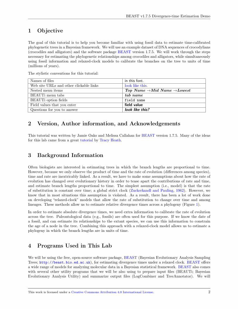
Often biologists are interested in estimating trees in which the branch lengths are proportional to time.However, because we only observe the product of time and the rate of evolution (differences among species),time and rate are inextricably linked. As a result, we have to make some assumptions about how the rate ofevolution has changed over evolutionary history in order to tease apart the contributions of rate and time,and estimate branch lengths proportional to time. The simplest assumption (i.e., model) is that the rateof substitution is constant over time; a global strict clock (Zuckerkandl and Pauling, 1962). However, weknow that in most situations this assumption is violated. As a result, there has been a lot of work doneon developing “relaxed-clock” models that allow the rate of substitution to change over time and amonglineages. These methods allow us to estimate relative divergence times across a phylogeny (Figure 1).

In order to estimate absolute divergence times, we need extra information to calibrate the rate of evolutionacross the tree. Paleontological data (e.g., fossils) are often used for this purpose. If we know the date ofa fossil, and can estimate its relationships to the extant species, we can use this information to constrainthe age of a node in the tree. Combining this approach with a relaxed-clock model allows us to estimate aphylogeny in which the branch lengths are in units of time.

4 Programs Used in This Lab

We will be using the free, open-source software package, BEAST (Bayesian Evolutionary Analysis SamplingTrees; http://beast.bio.ed.ac.uk), for estimating divergence times under a relaxed clock. BEAST offersa wide range of models for analyzing molecular data in a Bayesian statistical framework. BEAST also comeswith several other utility programs that we will be also using to prepare input files (BEAUTi; BayesianEvolutionary Analysis Utility) and summarize output files (LogCombiner and TreeAnnotator). We will



http://www.google.com


http://treethinkers.org/divergence-time-estimation-using-beast/

http://phylo.bio.ku.edu/content/tracy-heath


http://beast.bio.ed.ac.uk

http://beast.bio.ed.ac.uk





Figure 1: The branch lengths of a phylogenetic tree are the product of rate and time.

also be using the programs Tracer (http://tree.bio.ed.ac.uk/software/tracer) and FigTree (http://tree.bio.ed.ac.uk/software/figtree) for evaluating, summarizing, and viewing results.

5 The Data

We will be analyzing DNA sequence data from 24 species of crocodylians (crocodiles, alligators, caimans,and gharials). The sequences are from Oaks (2011), and encode the protein-coding cytochrome b genefrom the mitochondrial genome (this is a single gene from a larger multi-locus dataset that is availableat http://datadryad.org/resource/doi:10.5061/dryad.5k9s0. You can download a zip archive of thealigned sequence data and other auxiliary files used in this tutorial from http://www.phyletica.com/downloads/div-time-tutorial.zip.

For these data, a likelihood-ratio test rejects a global strict clock model. So, we will use an uncorrelatedlog-normally distributed (UCLD) relaxed-clock model (Drummond et al., 2006) to account for variation inrates of substitution across the tree in order to estimate branches proportional to time.

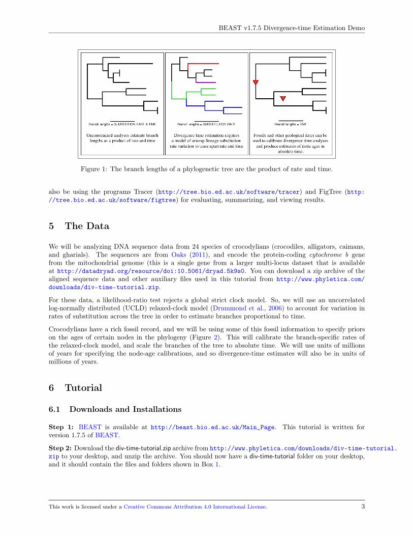
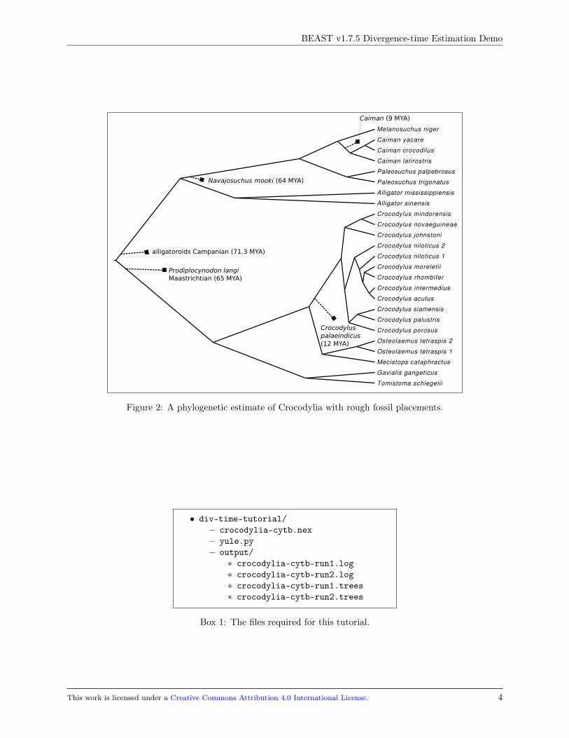
Crocodylians have a rich fossil record, and we will be using some of this fossil information to specify priorson the ages of certain nodes in the phylogeny (Figure 2). This will calibrate the branch-specific rates ofthe relaxed-clock model, and scale the branches of the tree to absolute time. We will use units of millionsof years for specifying the node-age calibrations, and so divergence-time estimates will also be in units ofmillions of years.

6 Tutorial

6.1 Downloads and Installations

Step 1: BEAST is available at http://beast.bio.ed.ac.uk/Main_Page. This tutorial is written forversion 1.7.5 of BEAST.

Step 2: Download the div-time-tutorial.zip archive from http://www.phyletica.com/downloads/div-time-tutorial.zip to your desktop, and unzip the archive. You should now have a div-time-tutorial folder on your desktop,and it should contain the files and folders shown in Box 1.


http://tree.bio.ed.ac.uk/software/tracer

http://tree.bio.ed.ac.uk/software/tracer

http://tree.bio.ed.ac.uk/software/figtree




http://datadryad.org/resource/doi:10.5061/dryad.5k9s0

http://datadryad.org/resource/doi:10.5061/dryad.5k9s0

http://www.phyletica.com/downloads/div-time-tutorial.zip














Melanosuchus niger

Tomistoma schlegelii

Caiman yacare

Crocodylus intermedius

Crocodylus palustris

Mecistops cataphractus

Alligator mississippiensis

Osteolaemus tetraspis 1

Alligator sinensis

Caiman crocodilus

Paleosuchus trigonatus

Crocodylus acutus

Crocodylus mindorensis

Crocodylus novaeguineae

Crocodylus porosus

Paleosuchus palpebrosus

Crocodylus niloticus 1

Crocodylus niloticus 2

Crocodylus rhombifer

Osteolaemus tetraspis 2

Caiman latirostris

Gavialis gangeticus

Crocodylus johnstoni

Crocodylus siamensis

Crocodylus moreletii

Navajosuchus mooki (64 MYA)

Prodiplocynodon langiMaastrichtian (65 MYA)

Caiman (9 MYA)

Crocodylus palaeindicus(12 MYA)

alligatoroids Campanian (71.3 MYA)

Figure 2: A phylogenetic estimate of Crocodylia with rough fossil placements.

• div-time-tutorial/– crocodylia-cytb.nex– yule.py– output/∗ crocodylia-cytb-run1.log∗ crocodylia-cytb-run2.log∗ crocodylia-cytb-run1.trees∗ crocodylia-cytb-run2.trees

Box 1: The files required for this tutorial.




6.2 Setting up XML file with BEAUTi

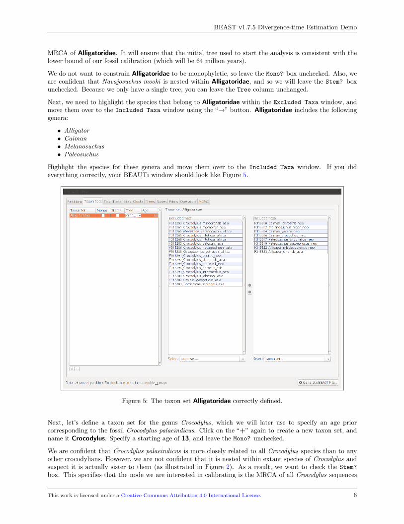
Step 3: Begin by launching the BEAUTi program. If you are using Mac OSX or Windows, you should beable to do this by double clicking on the application. If everything is working correctly, a window shouldappear that looks something like Figure 3.

Figure 3: BEAUTi window.

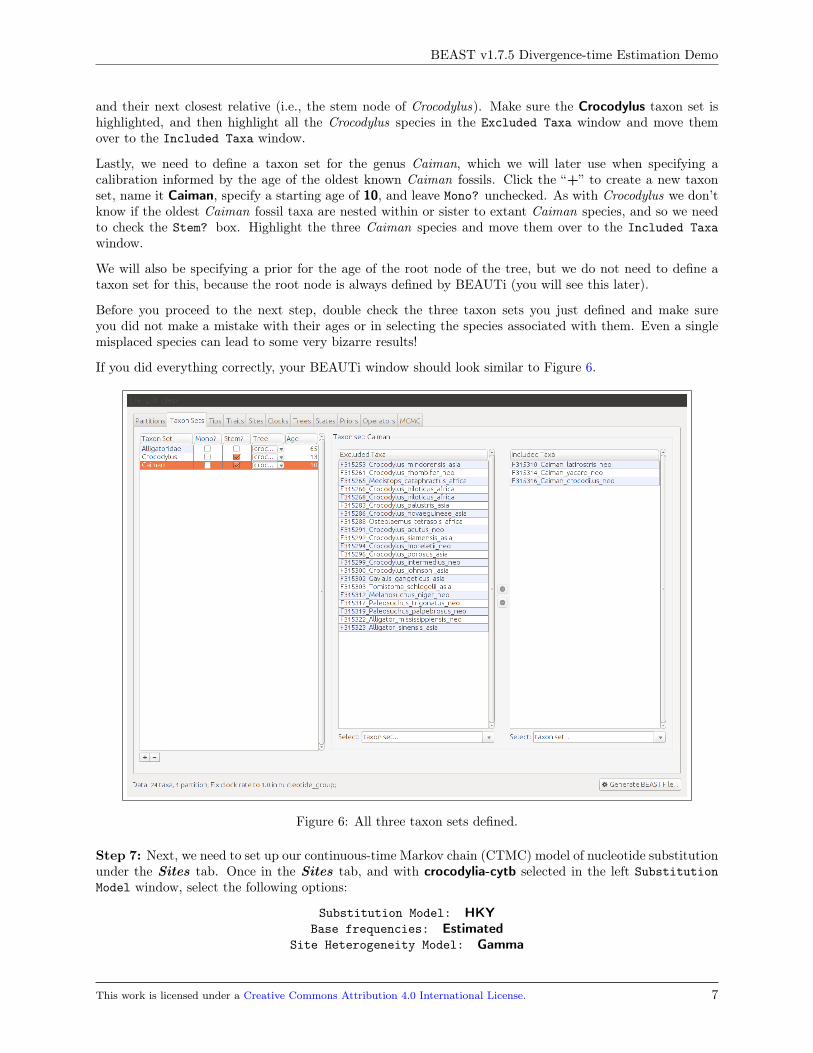
Step 4: Import the sequence data from the file crocodylia-cytb.nex using the drop-down menu File →ImportData or using the “+” button near the bottom-left corner of the window.

You should be able to confirm that BEAUTi successfully imported 24 sequences of nucleotides of length 1137(Figure 4).

Figure 4: The data successfully loaded by BEAUTi.

Step 5: Double click on the file name crocodylia-cytb.nex to bring up a window displaying the alignedsequences. It is always good practice to make sure everything looks as you expect. The cytochrome b geneis protein-coding, and aligns well across Crocodylia without gaps.

Step 6: Next, we need to define some sets of taxa. Later, we will be able to use each of these sets to placepriors on the age of their most recent common ancestor (MRCA). Let’s start by defining the set for the cladecontaining the fossil taxon Navajosuchus mooki ; this clade has the family name Alligatoridae.

Click on the Taxa tab. Once in the Taxa tab, click on the “+” near the bottom-left corner of the window.This will create an untitled taxon set in the left-most box in the window. Change the name of this taxonset to Alligatoridae and enter 65 into Age column. This age is simply a starting value for the age of the




MRCA of Alligatoridae. It will ensure that the initial tree used to start the analysis is consistent with thelower bound of our fossil calibration (which will be 64 million years).

We do not want to constrain Alligatoridae to be monophyletic, so leave the Mono? box unchecked. Also, weare confident that Navajosuchus mooki is nested within Alligatoridae, and so we will leave the Stem? boxunchecked. Because we only have a single tree, you can leave the Tree column unchanged.

Next, we need to highlight the species that belong to Alligatoridae within the Excluded Taxa window, andmove them over to the Included Taxa window using the “→” button. Alligatoridae includes the followinggenera:

• Alligator• Caiman• Melanosuchus• Paleosuchus

Highlight the species for these genera and move them over to the Included Taxa window. If you dideverything correctly, your BEAUTi window should look like Figure 5.

Figure 5: The taxon set Alligatoridae correctly defined.

Next, let’s define a taxon set for the genus Crocodylus, which we will later use to specify an age priorcorresponding to the fossil Crocodylus palaeindicus. Click on the “+” again to create a new taxon set, andname it Crocodylus. Specify a starting age of 13, and leave the Mono? unchecked.

We are confident that Crocodylus palaeindicus is more closely related to all Crocodylus species than to anyother crocodylians. However, we are not confident that it is nested within extant species of Crocodylus andsuspect it is actually sister to them (as illustrated in Figure 2). As a result, we want to check the Stem?box. This specifies that the node we are interested in calibrating is the MRCA of all Crocodylus sequences




and their next closest relative (i.e., the stem node of Crocodylus). Make sure the Crocodylus taxon set ishighlighted, and then highlight all the Crocodylus species in the Excluded Taxa window and move themover to the Included Taxa window.

Lastly, we need to define a taxon set for the genus Caiman, which we will later use when specifying acalibration informed by the age of the oldest known Caiman fossils. Click the “+” to create a new taxonset, name it Caiman, specify a starting age of 10, and leave Mono? unchecked. As with Crocodylus we don’tknow if the oldest Caiman fossil taxa are nested within or sister to extant Caiman species, and so we needto check the Stem? box. Highlight the three Caiman species and move them over to the Included Taxawindow.

We will also be specifying a prior for the age of the root node of the tree, but we do not need to define ataxon set for this, because the root node is always defined by BEAUTi (you will see this later).

Before you proceed to the next step, double check the three taxon sets you just defined and make sureyou did not make a mistake with their ages or in selecting the species associated with them. Even a singlemisplaced species can lead to some very bizarre results!

If you did everything correctly, your BEAUTi window should look similar to Figure 6.

Figure 6: All three taxon sets defined.

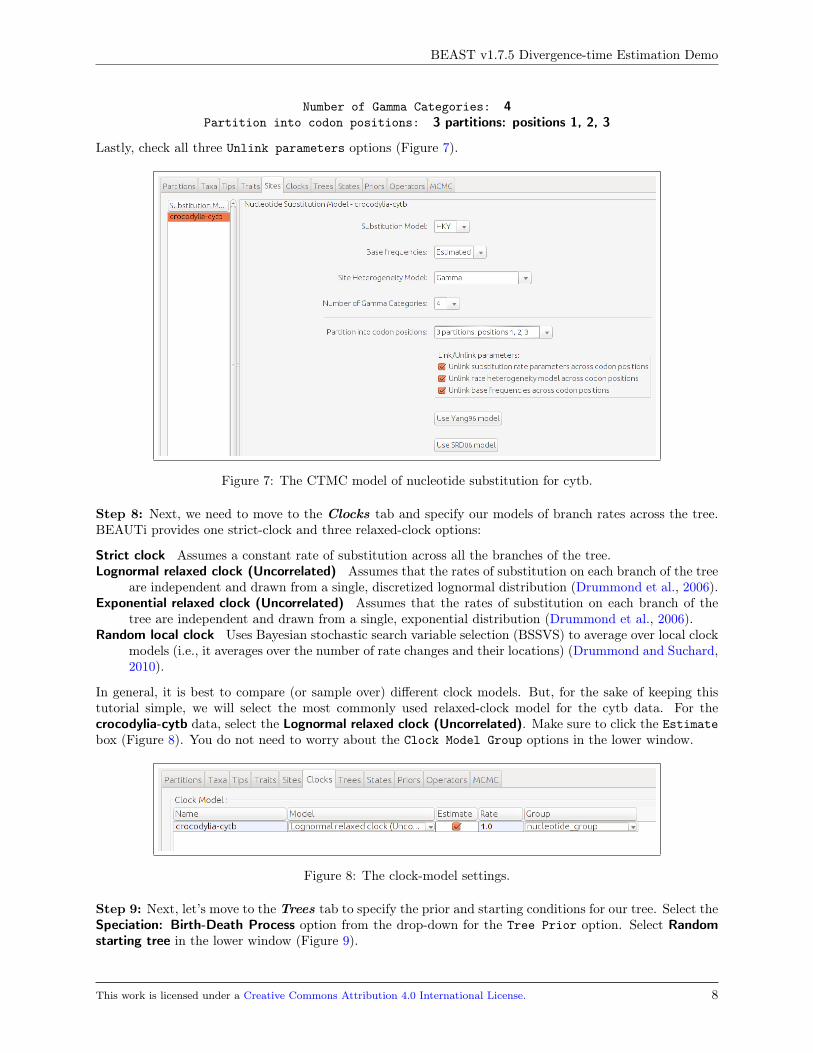
Step 7: Next, we need to set up our continuous-time Markov chain (CTMC) model of nucleotide substitutionunder the Sites tab. Once in the Sites tab, and with crocodylia-cytb selected in the left SubstitutionModel window, select the following options:

Substitution Model: HKYBase frequencies: Estimated

Site Heterogeneity Model: Gamma




Number of Gamma Categories: 4Partition into codon positions: 3 partitions: positions 1, 2, 3

Lastly, check all three Unlink parameters options (Figure 7).

Figure 7: The CTMC model of nucleotide substitution for cytb.

Step 8: Next, we need to move to the Clocks tab and specify our models of branch rates across the tree.BEAUTi provides one strict-clock and three relaxed-clock options:

Strict clock Assumes a constant rate of substitution across all the branches of the tree.Lognormal relaxed clock (Uncorrelated) Assumes that the rates of substitution on each branch of the tree

are independent and drawn from a single, discretized lognormal distribution (Drummond et al., 2006).Exponential relaxed clock (Uncorrelated) Assumes that the rates of substitution on each branch of the

tree are independent and drawn from a single, exponential distribution (Drummond et al., 2006).Random local clock Uses Bayesian stochastic search variable selection (BSSVS) to average over local clock

models (i.e., it averages over the number of rate changes and their locations) (Drummond and Suchard,2010).

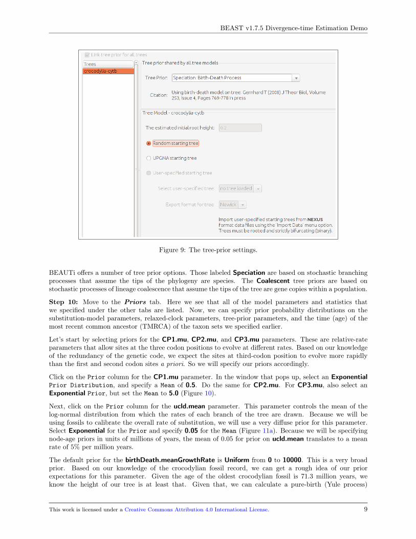
In general, it is best to compare (or sample over) different clock models. But, for the sake of keeping thistutorial simple, we will select the most commonly used relaxed-clock model for the cytb data. For thecrocodylia-cytb data, select the Lognormal relaxed clock (Uncorrelated). Make sure to click the Estimatebox (Figure 8). You do not need to worry about the Clock Model Group options in the lower window.

Figure 8: The clock-model settings.

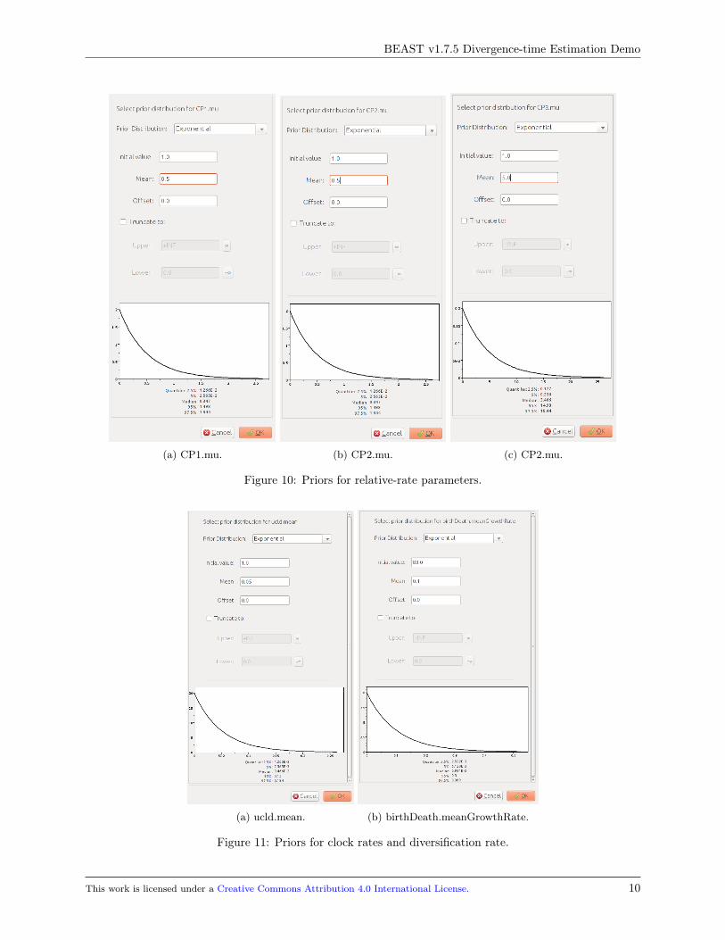
Step 9: Next, let’s move to the Trees tab to specify the prior and starting conditions for our tree. Select theSpeciation: Birth-Death Process option from the drop-down for the Tree Prior option. Select Randomstarting tree in the lower window (Figure 9).




Figure 9: The tree-prior settings.

BEAUTi offers a number of tree prior options. Those labeled Speciation are based on stochastic branchingprocesses that assume the tips of the phylogeny are species. The Coalescent tree priors are based onstochastic processes of lineage coalescence that assume the tips of the tree are gene copies within a population.

Step 10: Move to the Priors tab. Here we see that all of the model parameters and statistics thatwe specified under the other tabs are listed. Now, we can specify prior probability distributions on thesubstitution-model parameters, relaxed-clock parameters, tree-prior parameters, and the time (age) of themost recent common ancestor (TMRCA) of the taxon sets we specified earlier.

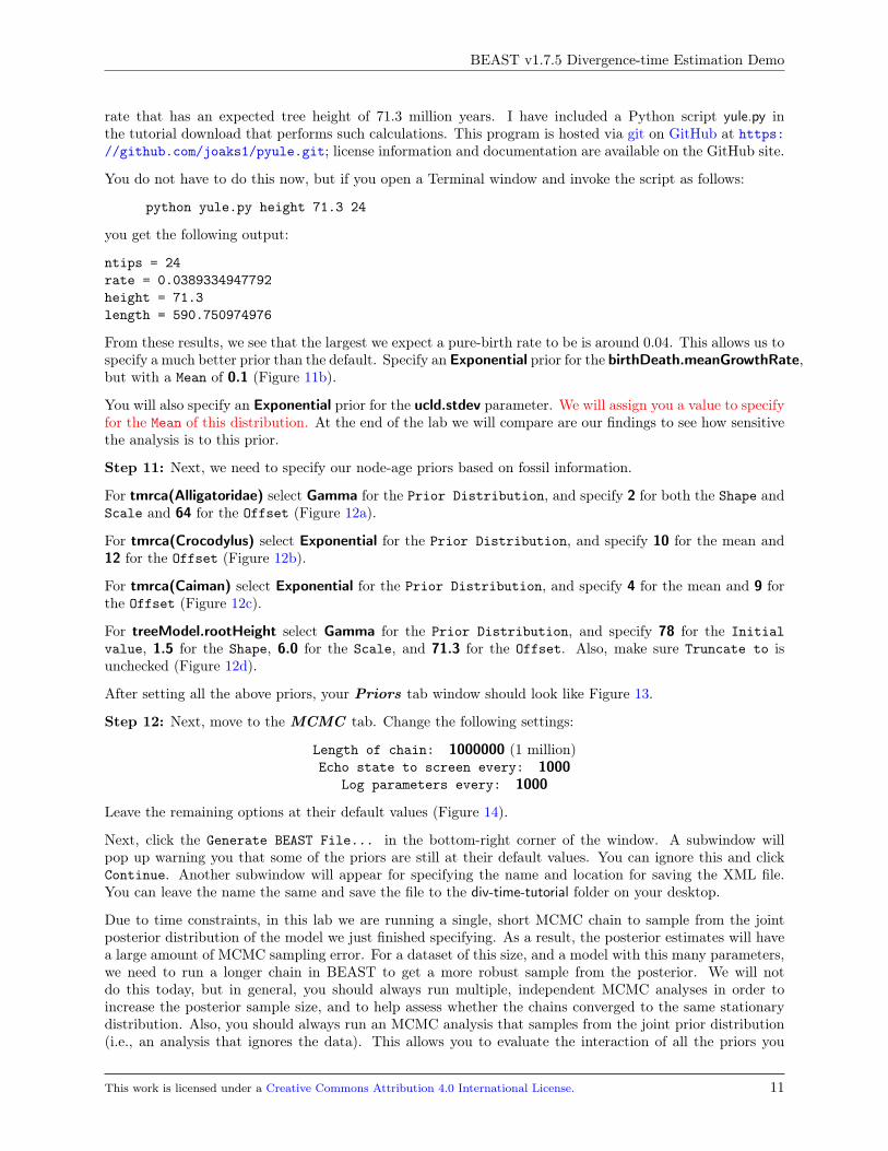
Let’s start by selecting priors for the CP1.mu, CP2.mu, and CP3.mu parameters. These are relative-rateparameters that allow sites at the three codon positions to evolve at different rates. Based on our knowledgeof the redundancy of the genetic code, we expect the sites at third-codon position to evolve more rapidlythan the first and second codon sites a priori. So we will specify our priors accordingly.

Click on the Prior column for the CP1.mu parameter. In the window that pops up, select an ExponentialPrior Distribution, and specify a Mean of 0.5. Do the same for CP2.mu. For CP3.mu, also select anExponential Prior, but set the Mean to 5.0 (Figure 10).

Next, click on the Prior column for the ucld.mean parameter. This parameter controls the mean of thelog-normal distribution from which the rates of each branch of the tree are drawn. Because we will beusing fossils to calibrate the overall rate of substitution, we will use a very diffuse prior for this parameter.Select Exponential for the Prior and specify 0.05 for the Mean (Figure 11a). Because we will be specifyingnode-age priors in units of millions of years, the mean of 0.05 for prior on ucld.mean translates to a meanrate of 5% per million years.

The default prior for the birthDeath.meanGrowthRate is Uniform from 0 to 10000. This is a very broadprior. Based on our knowledge of the crocodylian fossil record, we can get a rough idea of our priorexpectations for this parameter. Given the age of the oldest crocodylian fossil is 71.3 million years, weknow the height of our tree is at least that. Given that, we can calculate a pure-birth (Yule process)




(a) CP1.mu. (b) CP2.mu. (c) CP2.mu.

Figure 10: Priors for relative-rate parameters.

(a) ucld.mean. (b) birthDeath.meanGrowthRate.

Figure 11: Priors for clock rates and diversification rate.




rate that has an expected tree height of 71.3 million years. I have included a Python script yule.py inthe tutorial download that performs such calculations. This program is hosted via git on GitHub at https://github.com/joaks1/pyule.git; license information and documentation are available on the GitHub site.

You do not have to do this now, but if you open a Terminal window and invoke the script as follows:

python yule.py height 71.3 24

you get the following output:

ntips = 24rate = 0.0389334947792height = 71.3length = 590.750974976

From these results, we see that the largest we expect a pure-birth rate to be is around 0.04. This allows us tospecify a much better prior than the default. Specify an Exponential prior for the birthDeath.meanGrowthRate,but with a Mean of 0.1 (Figure 11b).

You will also specify an Exponential prior for the ucld.stdev parameter. We will assign you a value to specifyfor the Mean of this distribution. At the end of the lab we will compare are our findings to see how sensitivethe analysis is to this prior.

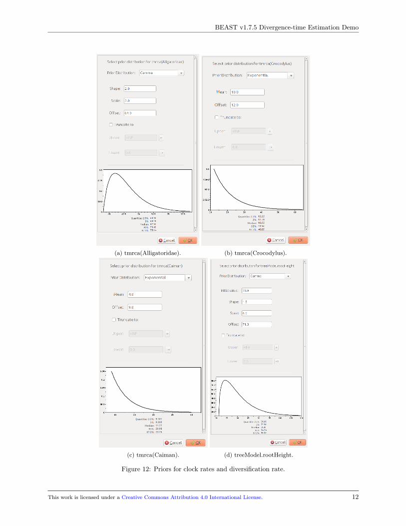
Step 11: Next, we need to specify our node-age priors based on fossil information.

For tmrca(Alligatoridae) select Gamma for the Prior Distribution, and specify 2 for both the Shape andScale and 64 for the Offset (Figure 12a).

For tmrca(Crocodylus) select Exponential for the Prior Distribution, and specify 10 for the mean and12 for the Offset (Figure 12b).

For tmrca(Caiman) select Exponential for the Prior Distribution, and specify 4 for the mean and 9 forthe Offset (Figure 12c).

For treeModel.rootHeight select Gamma for the Prior Distribution, and specify 78 for the Initialvalue, 1.5 for the Shape, 6.0 for the Scale, and 71.3 for the Offset. Also, make sure Truncate to isunchecked (Figure 12d).

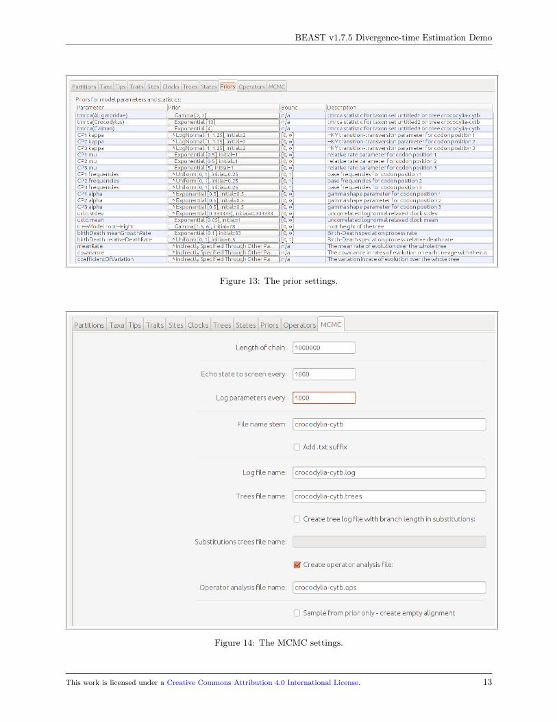
After setting all the above priors, your Priors tab window should look like Figure 13.

Step 12: Next, move to the MCMC tab. Change the following settings:

Length of chain: 1000000 (1 million)Echo state to screen every: 1000

Log parameters every: 1000

Leave the remaining options at their default values (Figure 14).

Next, click the Generate BEAST File... in the bottom-right corner of the window. A subwindow willpop up warning you that some of the priors are still at their default values. You can ignore this and clickContinue. Another subwindow will appear for specifying the name and location for saving the XML file.You can leave the name the same and save the file to the div-time-tutorial folder on your desktop.

Due to time constraints, in this lab we are running a single, short MCMC chain to sample from the jointposterior distribution of the model we just finished specifying. As a result, the posterior estimates will havea large amount of MCMC sampling error. For a dataset of this size, and a model with this many parameters,we need to run a longer chain in BEAST to get a more robust sample from the posterior. We will notdo this today, but in general, you should always run multiple, independent MCMC analyses in order toincrease the posterior sample size, and to help assess whether the chains converged to the same stationarydistribution. Also, you should always run an MCMC analysis that samples from the joint prior distribution(i.e., an analysis that ignores the data). This allows you to evaluate the interaction of all the priors you


http://git-scm.com/

https://github.com/

https://github.com/joaks1/pyule.git






(a) tmrca(Alligatoridae). (b) tmrca(Crocodylus).

(c) tmrca(Caiman). (d) treeModel.rootHeight.

Figure 12: Priors for clock rates and diversification rate.




Figure 13: The prior settings.

Figure 14: The MCMC settings.




have specified for the various parameters, and also gives you an idea of how much the data are influencingcertain parameter estimates. We will not do this today, but you do this by checking the Sample from prioronly-create empty alignment box and creating another XML file (make sure you change the name!).

Later, when your analysis is running, we will look at results from multiple, longer chains and from a chainthat sampled only from the prior.

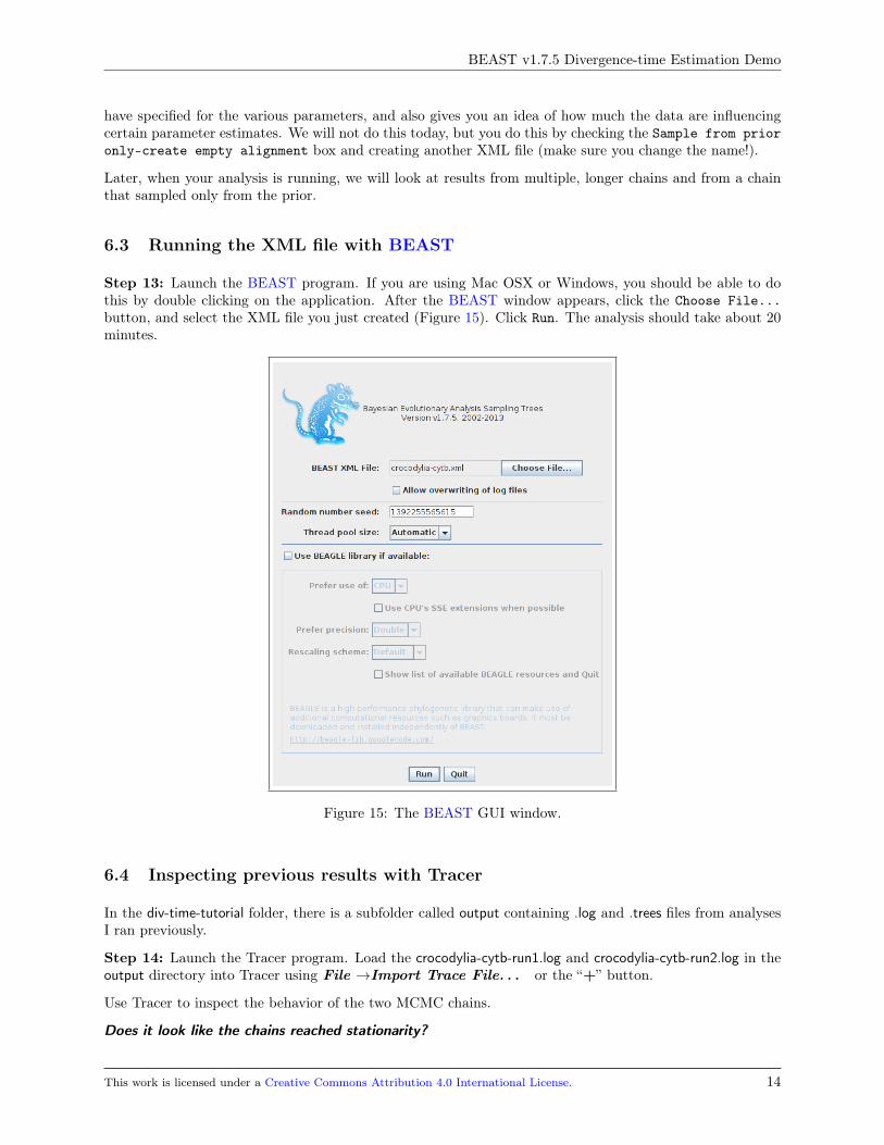
6.3 Running the XML file with BEAST

Step 13: Launch the BEAST program. If you are using Mac OSX or Windows, you should be able to dothis by double clicking on the application. After the BEAST window appears, click the Choose File...button, and select the XML file you just created (Figure 15). Click Run. The analysis should take about 20minutes.

Figure 15: The BEAST GUI window.

6.4 Inspecting previous results with Tracer

In the div-time-tutorial folder, there is a subfolder called output containing .log and .trees files from analysesI ran previously.

Step 14: Launch the Tracer program. Load the crocodylia-cytb-run1.log and crocodylia-cytb-run2.log in theoutput directory into Tracer using File →Import Trace File. . . or the “+” button.

Use Tracer to inspect the behavior of the two MCMC chains.

Does it look like the chains reached stationarity?








Does it look like both chains converged to the same stationarity distribution?

What do we call this stationary distribution?

Now, load the crocodylia-cytb-prior.log file into Tracer. This log file is from the analysis that sampled onlyfrom the prior distribution. Use Tracer to compare the prior and posterior samples.

Are any of the parameter estimates similar between the prior and posterior? Which ones?

6.5 Summarizing the trees with LogCombiner and TreeAnnotator

Once you have reviewed the log files from the independent runs in Tracer and determined that they havereached stationarity, you can combine the sampled trees into a single tree file.

Step 15: Launch the LogCombiner program. Change the File type: to Tree Files. Load the crocodylia-cytb-run1.trees and crocodylia-cytb-run2.trees file in the output directory into LogCombiner using the “+”button. Select the Choose File... button and specify the output directory and a file name, crocodylia-cytb-runs1and2.trees. Specify an appropriate burn-in value based on what you saw in Tracer. Click Run

Now you have a single tree file with all the trees from the two independent runs called crocodylia-cytb-runs1and2.trees. TreeAnnotator will summarize the trees and identify the topology with the best posteriorsupport, and summarize the age estimates for each node in the tree.

Step 16: Launch the TreeAnnotator program. Specify the burnin value as 0 (we removed the burn-in withLogCombiner). For the Target tree type field, choose Maximum clade credibility tree. For the Nodeheights field, choose Median heights. Select the Input Tree File button and select the file crocodylia-cytb-runs1and2.trees. Select the Output File button and specify the output directory and a file name,crocodylia-MCC.tre. Click Run




6.6 Visualizing the tree in FigTree

Step 17: Launch the FigTree program, and load the crocodylia-MCC.tre file you just created with TreeAn-notator. Check the Scale Axis option in the left column, and check the Scale Axis →Reverse axis box.Check the Node Bars option and select height_95%_HPD for the Node bars →Display field.

What is the age of the most recent common ancestor of all Crocodylus species?

What is the age of the stem node for Crocodylus?

6.7 Inspecting your results with Tracer

Step 18:

If your analysis has finished, launch the Tracer program and load the log file created by BEAST.

What was the mean you specified for the prior on ucld.stdev?

What is your estimate of the mean and 95% HPD interval for the age of the stem node for Crocodylus(hint: the tmrca(Crocodylus) statistic)?

Compare your estimate with your classmates that used a different prior on ucld.stdev. Are the resultssensitive to this prior? Is there a trend?




7 Quick Version of the Tutorial

Step 1: Download and install BEAST.

Step 2: Download the data and other files from Google Drive.

Step 3: Launch BEAUTi.

Step 4: Import the data in crocodylia-cytb.nex.

Step 5: Inspect the alignment.

Step 6: Define taxon sets.

Step 7: Define Markov-chain models of substitution

Step 8: Define clock models.

Step 9: Select the tree prior.

Step 10: Select priors for parameters.

Step 11: Select priors for node ages!

Step 12: Specify MCMC settings and generate BEAST XML files.

Step 13: Run the XML file in BEAST.

Step 14: Inspect previous results with Tracer.

Step 15: Combine tree files using LogCombiner.

Step 16: Summarize the trees using TreeAnnotator.

Step 17: Look at the summary tree in FigTree.

Step 18: Inspect the results of your short analysis with Tracer.







8 Additional Information/Resources

Great resources for divergence-time estimation include a tutorial and slides by Tracy Heath!


http://treethinkers.org/divergence-time-estimation-using-beast/

https://molevol.mbl.edu/wiki/images/6/6f/Bodega_2013_divtime_lecture.pdf

http://phylo.bio.ku.edu/content/tracy-heath



ReferencesDrummond, A. J., S. Y. W. Ho, M. J. Phillips, and A. Rambaut. 2006. Relaxed phylogenetics and datingwith confidence. PLoS Biology 4:e88.

Drummond, A. J. and M. A. Suchard. 2010. Bayesian random local clocks, or one rate to rule them all. BMCbiology 8:114.

Oaks, J. R. 2011. A time-calibrated species tree of Crocodylia reveals a recent radiation of the true crocodiles.Evolution 65:3285–3297.

Zuckerkandl, E. and L. Pauling. 1962. Molecular disease, evolution, and genetic heterogeneity. Pages 189–225in Horizons in Biochemistry (M. Kasha and B. Pullman, eds.). Academic Press, New York, USA.



Documents

BEAST Divergence-time Lab Contents - phyleticaphyletica.org/teaching/uw-biol-449/div-time-estimation/div-time... · BEAST Divergence-time Lab Contents ... The sequences are fromOaks(2011),