Embed Size (px)
DESCRIPTION
Beamerexample Conference Talk
Citation preview
Introduction Bad News: Hardness Results Good News: Tractability Results Summary
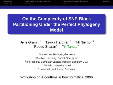
On the Complexity of SNP BlockPartitioning Under the Perfect Phylogeny
Model
Jens Gramm1 Tzvika Hartman2 Till Nierhoff3
Roded Sharan4 Till Tantau5
1Universität Tübingen, Germany2Bar-Ilan University, Ramat-Gan, Israel
3International Computer Science Institute, Berkeley, USA4Tel-Aviv University, Israel
5Universität zu Lübeck, Germany
Workshop on Algorithms in Bioinformatics, 2006
Introduction Bad News: Hardness Results Good News: Tractability Results Summary
Outline
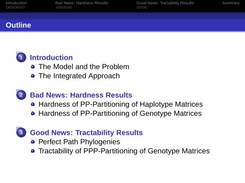
1 IntroductionThe Model and the ProblemThe Integrated Approach
2 Bad News: Hardness ResultsHardness of PP-Partitioning of Haplotype MatricesHardness of PP-Partitioning of Genotype Matrices
3 Good News: Tractability ResultsPerfect Path PhylogeniesTractability of PPP-Partitioning of Genotype Matrices
Introduction Bad News: Hardness Results Good News: Tractability Results Summary
The Model and the Problem
What is haplotyping and why is it important?
You hopefully know this after the previous three talks. . .
Introduction Bad News: Hardness Results Good News: Tractability Results Summary
The Model and the Problem
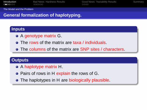
General formalization of haplotyping.
Inputs
A genotype matrix G.
The rows of the matrix are taxa / individuals.
The columns of the matrix are SNP sites / characters.
Outputs
A haplotype matrix H.
Pairs of rows in H explain the rows of G.
The haplotypes in H are biologically plausible.
Introduction Bad News: Hardness Results Good News: Tractability Results Summary
The Model and the Problem
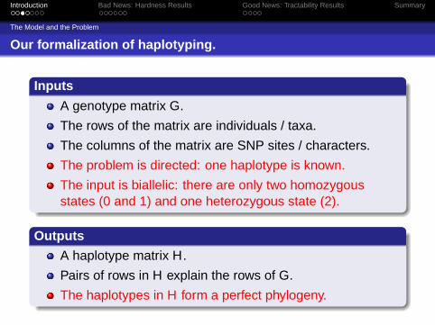
Our formalization of haplotyping.
Inputs
A genotype matrix G.
The rows of the matrix are individuals / taxa.
The columns of the matrix are SNP sites / characters.
The problem is directed: one haplotype is known.
The input is biallelic: there are only two homozygousstates (0 and 1) and one heterozygous state (2).
Outputs
A haplotype matrix H.
Pairs of rows in H explain the rows of G.
The haplotypes in H form a perfect phylogeny.
Introduction Bad News: Hardness Results Good News: Tractability Results Summary
The Model and the Problem
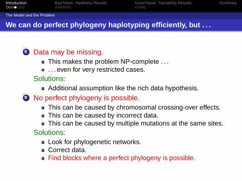
We can do perfect phylogeny haplotyping efficiently, but . . .
1 Data may be missing.This makes the problem NP-complete . . .. . . even for very restricted cases.
Solutions:Additional assumption like the rich data hypothesis.
2 No perfect phylogeny is possible.This can be caused by chromosomal crossing-over effects.This can be caused by incorrect data.This can be caused by multiple mutations at the same sites.
Solutions:Look for phylogenetic networks.Correct data.Find blocks where a perfect phylogeny is possible.
Introduction Bad News: Hardness Results Good News: Tractability Results Summary
The Integrated Approach
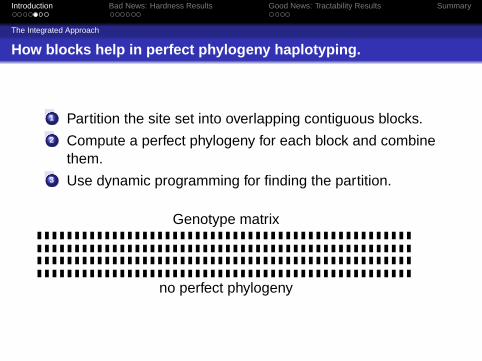
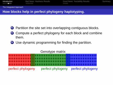
How blocks help in perfect phylogeny haplotyping.
1 Partition the site set into overlapping contiguous blocks.2 Compute a perfect phylogeny for each block and combine
them.3 Use dynamic programming for finding the partition.
Genotype matrix
no perfect phylogeny
Introduction Bad News: Hardness Results Good News: Tractability Results Summary
The Integrated Approach
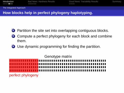
How blocks help in perfect phylogeny haplotyping.
1 Partition the site set into overlapping contiguous blocks.2 Compute a perfect phylogeny for each block and combine
them.3 Use dynamic programming for finding the partition.
Genotype matrix
perfect phylogeny
Introduction Bad News: Hardness Results Good News: Tractability Results Summary
The Integrated Approach
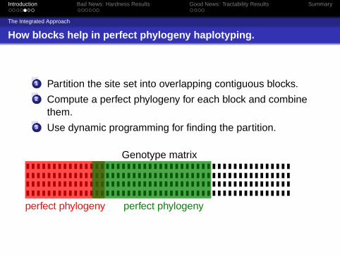
How blocks help in perfect phylogeny haplotyping.
1 Partition the site set into overlapping contiguous blocks.2 Compute a perfect phylogeny for each block and combine
them.3 Use dynamic programming for finding the partition.
Genotype matrix
perfect phylogeny perfect phylogeny
Introduction Bad News: Hardness Results Good News: Tractability Results Summary
The Integrated Approach
How blocks help in perfect phylogeny haplotyping.
1 Partition the site set into overlapping contiguous blocks.2 Compute a perfect phylogeny for each block and combine
them.3 Use dynamic programming for finding the partition.
Genotype matrix
perfect phylogeny perfect phylogeny perfect phylogeny
Introduction Bad News: Hardness Results Good News: Tractability Results Summary
The Integrated Approach
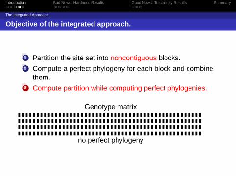
Objective of the integrated approach.
1 Partition the site set into noncontiguous blocks.2 Compute a perfect phylogeny for each block and combine
them.3 Compute partition while computing perfect phylogenies.
Genotype matrix
no perfect phylogeny
Introduction Bad News: Hardness Results Good News: Tractability Results Summary
The Integrated Approach
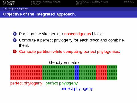
Objective of the integrated approach.
1 Partition the site set into noncontiguous blocks.2 Compute a perfect phylogeny for each block and combine
them.3 Compute partition while computing perfect phylogenies.
Genotype matrix
perfect phylogeny perfect phylogenyperfect phylogeny
Introduction Bad News: Hardness Results Good News: Tractability Results Summary
The Integrated Approach
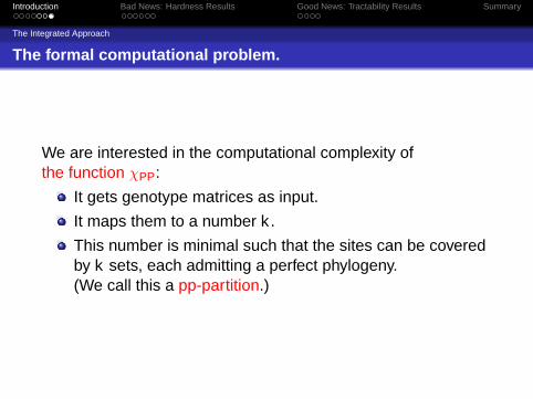
The formal computational problem.
We are interested in the computational complexity ofthe function χPP:
It gets genotype matrices as input.
It maps them to a number k .
This number is minimal such that the sites can be coveredby k sets, each admitting a perfect phylogeny.(We call this a pp-partition.)
Introduction Bad News: Hardness Results Good News: Tractability Results Summary
Hardness of PP-Partitioning of Haplotype Matrices
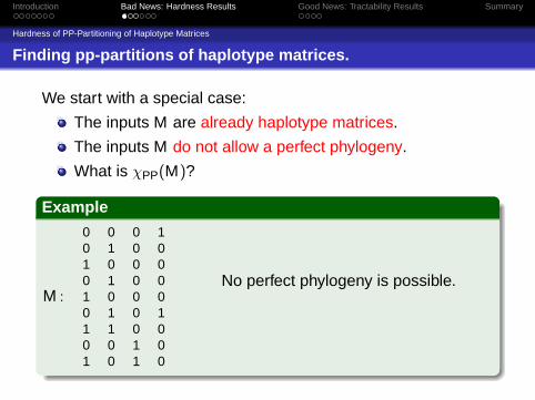
Finding pp-partitions of haplotype matrices.
We start with a special case:
The inputs M are already haplotype matrices.
The inputs M do not allow a perfect phylogeny.
What is χPP(M)?
Example
M :
0 0 0 10 1 0 01 0 0 00 1 0 01 0 0 00 1 0 11 1 0 00 0 1 01 0 1 0
No perfect phylogeny is possible.
Introduction Bad News: Hardness Results Good News: Tractability Results Summary
Hardness of PP-Partitioning of Haplotype Matrices
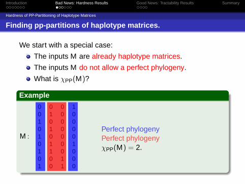
Finding pp-partitions of haplotype matrices.
We start with a special case:
The inputs M are already haplotype matrices.
The inputs M do not allow a perfect phylogeny.
What is χPP(M)?
Example
M :
0 0 0 10 1 0 01 0 0 00 1 0 01 0 0 00 1 0 11 1 0 00 0 1 01 0 1 0
Perfect phylogenyPerfect phylogenyχPP(M) = 2.
Introduction Bad News: Hardness Results Good News: Tractability Results Summary
Hardness of PP-Partitioning of Haplotype Matrices
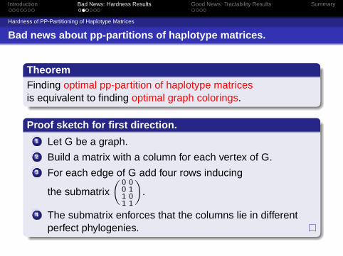
Bad news about pp-partitions of haplotype matrices.
TheoremFinding optimal pp-partition of haplotype matricesis equivalent to finding optimal graph colorings.
Proof sketch for first direction.1 Let G be a graph.2 Build a matrix with a column for each vertex of G.3 For each edge of G add four rows inducing
the submatrix( 0 0
0 11 01 1
).
4 The submatrix enforces that the columns lie in differentperfect phylogenies.
Introduction Bad News: Hardness Results Good News: Tractability Results Summary
Hardness of PP-Partitioning of Haplotype Matrices
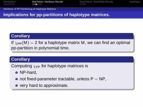
Implications for pp-partitions of haplotype matrices.
Corollary
If χPP(M) = 2 for a haplotype matrix M, we can find an optimalpp-partition in polynomial time.
Corollary
Computing χPP for haplotype matrices is
NP-hard,
not fixed-parameter tractable, unless P = NP,
very hard to approximate.
Introduction Bad News: Hardness Results Good News: Tractability Results Summary
Hardness of PP-Partitioning of Genotype Matrices
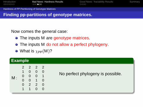
Finding pp-partitions of genotype matrices.
Now comes the general case:
The inputs M are genotype matrices.
The inputs M do not allow a perfect phylogeny.
What is χPP(M)?
Example
M :
2 2 2 21 0 0 00 0 0 10 0 1 00 2 2 01 1 0 0
No perfect phylogeny is possible.
Introduction Bad News: Hardness Results Good News: Tractability Results Summary
Hardness of PP-Partitioning of Genotype Matrices
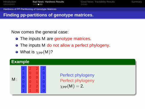
Finding pp-partitions of genotype matrices.
Now comes the general case:
The inputs M are genotype matrices.
The inputs M do not allow a perfect phylogeny.
What is χPP(M)?
Example
M :
2 2 2 21 0 0 00 0 0 10 0 1 00 2 2 01 1 0 0
Perfect phylogenyPerfect phylogenyχPP(M) = 2.
Introduction Bad News: Hardness Results Good News: Tractability Results Summary
Hardness of PP-Partitioning of Genotype Matrices
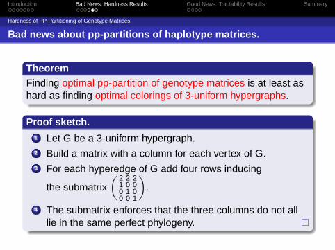
Bad news about pp-partitions of haplotype matrices.
TheoremFinding optimal pp-partition of genotype matrices is at least ashard as finding optimal colorings of 3-uniform hypergraphs.
Proof sketch.1 Let G be a 3-uniform hypergraph.2 Build a matrix with a column for each vertex of G.3 For each hyperedge of G add four rows inducing
the submatrix( 2 2 2
1 0 00 1 00 0 1
).
4 The submatrix enforces that the three columns do not alllie in the same perfect phylogeny.
Introduction Bad News: Hardness Results Good News: Tractability Results Summary
Hardness of PP-Partitioning of Genotype Matrices
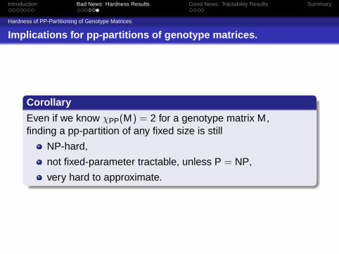
Implications for pp-partitions of genotype matrices.
Corollary
Even if we know χPP(M) = 2 for a genotype matrix M,finding a pp-partition of any fixed size is still
NP-hard,
not fixed-parameter tractable, unless P = NP,
very hard to approximate.
Introduction Bad News: Hardness Results Good News: Tractability Results Summary
Perfect Path Phylogenies
Automatic optimal pp-partitioning is hopeless, but. . .
The hardness results are worst-case results forhighly artificial inputs.
Real biological data might have special properties thatmake the problem tractable.
One such property is that perfect phylogenies are oftenperfect path phylogenies:In HapMap data, in 70% of the blocks where a perfectphylogeny is possible a perfect path phylogeny is alsopossible.
Introduction Bad News: Hardness Results Good News: Tractability Results Summary
Perfect Path Phylogenies
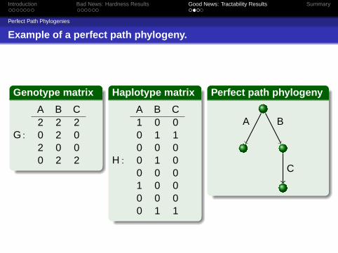
Example of a perfect path phylogeny.
Genotype matrix
G :
A B C2 2 20 2 02 0 00 2 2
Haplotype matrix
H :
A B C1 0 00 1 10 0 00 1 00 0 01 0 00 0 00 1 1
Perfect path phylogeny
A
C
B
Introduction Bad News: Hardness Results Good News: Tractability Results Summary
Perfect Path Phylogenies
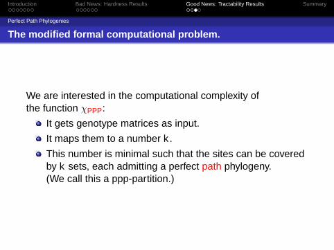
The modified formal computational problem.
We are interested in the computational complexity ofthe function χPPP:
It gets genotype matrices as input.
It maps them to a number k .
This number is minimal such that the sites can be coveredby k sets, each admitting a perfect path phylogeny.(We call this a ppp-partition.)
Introduction Bad News: Hardness Results Good News: Tractability Results Summary
Tractability of PPP-Partitioning of Genotype Matrices
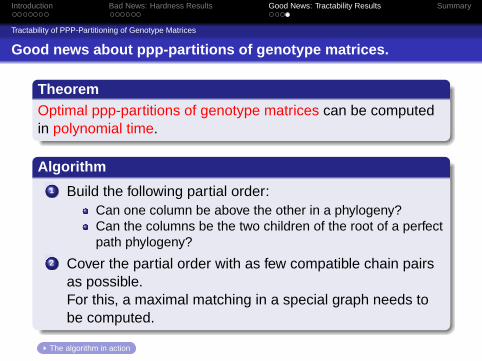
Good news about ppp-partitions of genotype matrices.
TheoremOptimal ppp-partitions of genotype matrices can be computedin polynomial time.
Algorithm
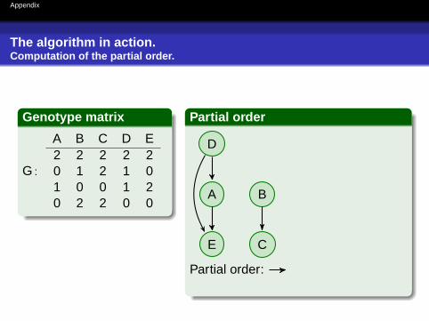
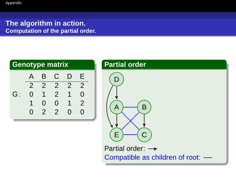
1 Build the following partial order:Can one column be above the other in a phylogeny?Can the columns be the two children of the root of a perfectpath phylogeny?
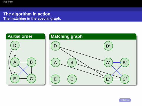
2 Cover the partial order with as few compatible chain pairsas possible.For this, a maximal matching in a special graph needs tobe computed.
The algorithm in action
Introduction Bad News: Hardness Results Good News: Tractability Results Summary
Summary
Finding optimal pp-partitions is intractable.
It is even intractable to find a pp-partition when just twononcontiguous blocks are known to suffice.
For perfect path phylogenies, optimal partitions can becomputed in polynomial time.
Appendix
The algorithm in action.Computation of the partial order.
Genotype matrix
G :
A B C D E2 2 2 2 20 1 2 1 01 0 0 1 20 2 2 0 0
Partial order
A B
C
D
E
Partial order:
Compatible as children of root:
Appendix
The algorithm in action.Computation of the partial order.
Genotype matrix
G :
A B C D E2 2 2 2 20 1 2 1 01 0 0 1 20 2 2 0 0
Partial order
A B
C
D
E
Partial order:Compatible as children of root:
Appendix
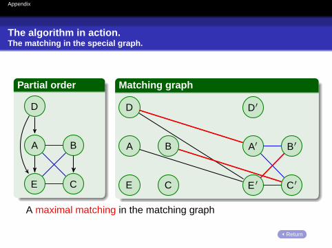
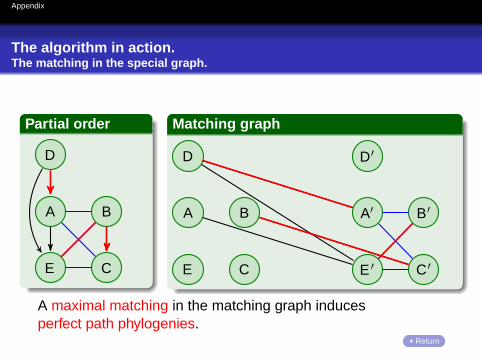
The algorithm in action.The matching in the special graph.
Partial order
A B
C
D
E
Matching graph
A B
C
D
E
A′ B′
C′
D′
E ′
A maximal matching in the matching graph
inducesperfect path phylogenies.
Return
Appendix
The algorithm in action.The matching in the special graph.
Partial order
A B
C
D
E
Matching graph
A B
C
D
E
A′ B′
C′
D′
E ′
A maximal matching in the matching graph
inducesperfect path phylogenies.
Return
Appendix
The algorithm in action.The matching in the special graph.
Partial order
A B
C
D
E
Matching graph
A B
C
D
E
A′ B′
C′
D′
E ′
A maximal matching in the matching graph inducesperfect path phylogenies.
Return