arX

iv:h

ep-e

x/02

1203

7v1

16

Dec

200

2

Beam Test of Silicon Strip Sensors for the

ZEUS Micro Vertex Detector

L.A.T. Bauerdick 1(a), E. Borsato 2, C. Burgard 1, T. Carli 1, R. Carlin 2,

M. Casaro 2, V. Chiochia 1, F. Dal Corso 2, D. Dannheim 1, A. Garfagnini 5(b),

A. Kappes 3, R. Klanner 5, E. Koffeman 4, B. Koppitz 5, U. Kotz 1, E. Maddox 4,

M. Milite 1(c)∗, M. Moritz 1, J.S.T. Ng 1(d), M.C. Petrucci 1, I. Redondo 6(e)∗,

J. Rautenberg 3(f), H. Tiecke 4, M. Turcato 2, J.J. Velthuis 4, A. Weber 3

(1) Deutsches Elektronen-Synchrotron DESY, Hamburg, Germany

(2) Dipartimento di Fisica dell’ Universita and INFN, Padova, Italy

(3) Physikalisches Institut der Universitat Bonn, Bonn, Germany

(4) NIKHEF and University of Amsterdam, Amsterdam, Netherlands

(5) Hamburg University, Institute of Exp. Physics, Hamburg, Germany

(6) Universidad Autonoma de Madrid, Madrid, Spain

(a) Now at Fermi National Accelerator Laboratory FNAL, Batavia, Illinois, USA

(b) Now at Dipartimento di Fisica dell’ Universita and INFN, Padova, Italy

(c) Now at Hamburg University, Institute of Exp. Physics, Hamburg, Germany

(d) Now at the Stanford Linear Accelerator Center SLAC, Stanford, California,

USA

(e) Now at Laboratoire Leprince Ringuet - Ecole Polytechnique, Route de Saclay

91128 Palaiseau Cedex, France

(f) Supported by the GIF, contract I-523-13.7/97.

* Corresponding authors. Tel: +33 1 69 33 44 05 ; fax:+33 1 69 33 30 02

E−mail addresses : redondo@poly.in2p3.fr (I. Redondo), milite@mail.desy.de

(M. Milite).

Preprint submitted to Elsevier Science 23 October 2018

Abstract

For the HERA upgrade, the ZEUS experiment has designed and installed a high

precision Micro Vertex Detector (MVD) using single sided µ-strip sensors with ca-

pacitive charge division. The sensors have a readout pitch of 120 µm, with five

intermediate strips (20 µm strip pitch). An extensive test program has been carried

out at the DESY-II testbeam facility. In this paper we describe the setup devel-

oped to test the ZEUS MVD sensors and the results obtained on both irradiated

and non-irradiated single sided µ-strip detectors with rectangular and trapezoidal

geometries. The performances of the sensors coupled to the readout electronics (HE-

LIX chip, version 2.2) have been studied in detail, achieving a good description by

a Monte Carlo simulation. Measurements of the position resolution as a function

of the angle of incidence are presented, focusing in particular on the comparison

between standard and newly developed reconstruction algorithms.

PACS : 29.40.Gx; 29.40.Wk; 07.05.kj

Keywords : ZEUS; Beam test; Silicon; Microstrip; Position reconstruction algo-

rithms

1 Introduction

The HERA ep collider luminosity upgrade [1] performed during the years 2000-

2001 aims to increase the instantaneous luminosity from 1.5 to 6 · 1031 cm−2

s−1, providing thus a higher sensitivity to low cross section physics. The ZEUS

experiment [2] has been equipped with a new silicon Micro Vertex Detector

(MVD) which is going to improve the global precision of the existing tracking

system, allowing to identify events with secondary vertices coming from the

decay of long-lived states such as hadrons with charm or bottom and τ leptons.

Moreover, the detector acceptance will be enhanced in the forward region,

2

along the proton beam direction, improving for example the detection of very

high Q2 scattered electrons and the reconstruction of the interaction vertex in

high x charged current events 1 .

According to the design specifications [3, 4, 5, 6], the MVD is composed of a

barrel (BMVD) and forward (FMVD) part, requiring a good matching with

the existing detectors. The MVD had to fit inside a cylinder of 324 mm diam-

eter defined by the inner wall of the Central Tracking Detector (CTD). The

readout electronics, based on the HELIX chip (version 3.0) [7, 8] is mounted

inside the active area, close to the silicon diodes. The silicon sensors are single

sided, AC coupled, strip detectors with capacitive charge division; the readout

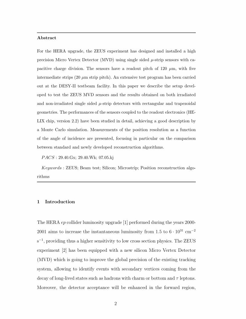
pitch is 120 µm and the strip pitch is 20 µm. A sketch of the silicon sensor can

be seen in figure 1. The BMVD (FMVD-1,FMVD-2) sensors have a rectangu-

lar (trapezoidal) geometry with 6.4 cm x 6.4 cm (base=6.4 cm × height=7.35

cm and 6.4 cm ×4.85 cm, respectively) dimensions. In the FMVD, the sides

of the trapezoid are tilted by 180/14 with respect to the bases and the strips

are parallel to one of the tilted sides of the trapezoid, having thus different

lengths across the sensor. The biasing of the strips is implemented using poly-

silicon resistors (∼ 1.5-2.5 MΩ) connected to the sensor ground line (called in

the following biasing ring), located alternatively on both ends of the strips.

The first and last strips close the biasing ring, being directly connected to it.

Three p+ guard rings, designed to adjust the potential towards the detector

edges, surround the sensitive area. An additional n+ doped implant beyond

the last guard ring allows to bias the backplane with a contact from the top.

Detailed descriptions of the MVD design and mechanical structure can be

found in [5,9,10,11]. The detailed design of the silicon sensors and results on

1 −Q2 is the exchanged photon invariant mass; x is the fraction of the proton

momentum carried by the struck quark.

3

the electrical measurements are described elsewhere [12, 13, 14].

The testbeam program for the MVD had several goals:

• to study the general performance of sensors with minimum ionising particles

(i.e. noise level, pedestal stability, hit efficiency, charge division);

• to test prototype versions of frontend electronics (i.e. readout chips and

hybrids) ;

• to test the sensors at different bias voltages;

• to measure the position resolution for different angles of incidence in order

to optimise reconstruction algorithms;

• to study the effect of irradiation.

The data have been compared with the results of a Monte Carlo program for

the silicon sensor simulation in order to gain input for the vertex detector

simulation. The detector performances have been studied using three non-

irradiated and two additional irradiated sensors [15, 14]. A barrel sensor was

irradiated using photons from a 60Co source: the detector was left floating

and irradiated up to an integrated dose of 2.0 kGy. A second sensor was

irradiated with reactor neutrons having a fluency φe = 1013 1 MeVequiv. n/cm2.

No substantial effects due to radiation damage on the detector performances

have been observed. All results presented in the following sections refer to

non-irradiated sensors and to the sensor irradiated floating with 2 kGy of

60Co photons.

After a brief description of the testbeam setup in section 2, the treatment

of the data and the general performance of the detectors are summarised

in section 3. The detector simulation is described in section 4. Section 5

is devoted to studies which use perpendicular tracks. It also describes the

extraction of the intrinsic position resolution. The position resolution as a

4

n+

~0.6µmSi3N4

Al

SiO2

n

120µm

SiO2-passivation

1.5µm14µm

Al

300µm

p+

20µm

12µm

C

CC

b

ii

ionizing particle

s25000cos

Q ~ e

h

CC

Ql Q (1 - s / 120)~ Qr Q s / 120~

e - h pairsθ θ

Fig. 1. Cross section of a MVD silicon sensor between two readout strips (drawing

not to scale). Dimensions of the layers are given in the left part of the picture. On

the right side a simplified picture of the capacitive network is shown.

function of the angle of incidence is studied in detail in sections 6 and 7. The

paper ends with a summary of the results.

2 Test beam setup

The measurements were performed at the DESY-II testbeam, a parasitic elec-

tron beam obtained after two conversions: a 10 µm thick carbon-fiber target

in the machine intercepts the beam and produces bremsstrahlung photons

which are converted into electron-positron pairs in a 0.1 X0 thick copper tar-

get. A bending magnet together with a momentum defining collimator slit

delivers the beam into the experimental hall. Depending on the primary use

of DESY-II the maximal momentum varies between 4.3 and 7.5 GeV/c. Most

measurements were done at 3 and 6 GeV/c resulting in a trigger rate of ∼ 10

Hz and ∼ 2 Hz, respectively.

A silicon reference telescope has been assembled to allow a precise determi-

nation of the particle impact point on the detector to be studied. Both, the

telescope modules and the module holding the MVD detector are mounted

5

300

m µ

= 0θ θ~ 35

120 mµ

φ

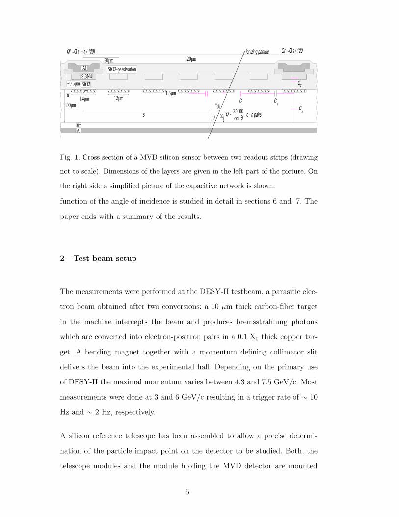
Fig. 2. Schematic cross section of a MVD silicon sensor to scale. The angles of

incidence θ and φ are indicated.

on a common optical bench. The detector to be studied is mounted between

the telescope modules on linear and rotational positioners which allow to in-

vestigate the performance in different areas of the detector and for different

angles of incidence. The rotations can be around the strip axis (θ angle) or

around the axis perpendicular to the strip in the detector plane (φ angle) (see

figure 2). A trigger was generated by coincidence of the signals from scintil-

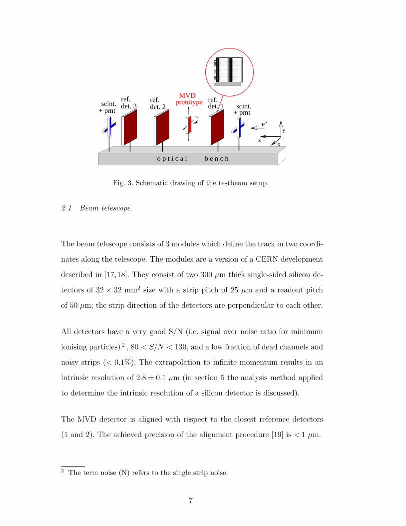
lator fingers located at both end sides of the optical bench. A drawing of the

testbeam setup is shown in figure 3. The data acquisition system is based on

an embedded Sun workstation in a VME-crate which controls the initialisa-

tion of the readout modules, the readout chips, the pattern generators, the

GPIB-interface for the positioners and the data taking. The system is run

under LabView [16].

6

b e n c ho p t i c a l

+ pmtscint. scint.

ref.det. 1

+ pmtdet. 2ref.

det. 3ref.

x

y

z

e-

prototypeMVD

Fig. 3. Schematic drawing of the testbeam setup.

2.1 Beam telescope

The beam telescope consists of 3 modules which define the track in two coordi-

nates along the telescope. The modules are a version of a CERN development

described in [17,18]. They consist of two 300 µm thick single-sided silicon de-

tectors of 32 × 32 mm2 size with a strip pitch of 25 µm and a readout pitch

of 50 µm; the strip direction of the detectors are perpendicular to each other.

All detectors have a very good S/N (i.e. signal over noise ratio for minimum

ionising particles) 2 , 80 < S/N < 130, and a low fraction of dead channels and

noisy strips (< 0.1%). The extrapolation to infinite momentum results in an

intrinsic resolution of 2.8 ± 0.1 µm (in section 5 the analysis method applied

to determine the intrinsic resolution of a silicon detector is discussed).

The MVD detector is aligned with respect to the closest reference detectors

(1 and 2). The achieved precision of the alignment procedure [19] is < 1 µm.

2 The term noise (N) refers to the single strip noise.

7

2.2 MVD detector readout

The MVD detectors were operated in the test beam using prototype versions of

the HELIX readout chip (version 2.2), developed for the Hera-B experiment [7,

8]. The HELIX chip provides 128 analog channels with a charge sensitive pre-

amplifier and shaper, forming a semi-Gaussian pulse with a peaking time of

∼ 50-70 ns. The signals are sampled in an analog pipeline capable of storing

128 events with 8 extra channels for trigger derandomisation. The chip can

be operated up to 40 MHz clock-rate. In the ZEUS experiment it will be used

at 10 MHz write and read speed. In order to simplify the readout system in

the testbeam, it was decided to synchronise the chip clock to the synchrotron

revolution frequency of about 1.05 MHz; with this setting particles traversing

the detectors were in a fixed phase relation to the chip clock. Tests performed

using a frequency multiplier of 10 (which are not discussed in the present

paper) showed no difference in the detector performances.

2.3 MVD detector assembly

In the testbeam, a protection circuit, including a protection resistance of 0.5

MΩ, was introduced between the backplane contact and the power supply. In

the following, the voltage applied between the biasing ring and the backplane

is referred to as Vbias. The detectors were biased at full depletion, unless

otherwise stated. The Barrel and Forward MVD detectors are connected to the

front-end electronics using a Upilex [20] “fan-out” foil with conductive lines.

The Upilex circuits are made of an Upilex S substrate, a 50 µm thick polyimide

film. A conductive layer of 5 µm electro-plated copper is deposited on top

and separated from the substrate by means of a 150 nm thick nickel adhesion

layer. A 1.5 µm gold layer is deposited over the conductive strips and the pads

8

used for bonding. The Upilex circuits for the Barrel and Forward modules are

produced at CERN [21]. The strip pitch is 120 µm on the detector side and

is reduced to 100 µm on the hybrid, where the Upilex strips are connected

to a pitch adapter which further reduces the readout pitch to 41.4 µm of the

HELIX input bond pads. The front-end electronic is mounted on a multi-layer

Hybrid structure (40 × 70 cm2) supporting 4 HELIX chips which are needed

to read-out the 512 strips of a BMVD detector; for the FMVD detector only

480 readout channels are required.

3 Data analysis and general performance

The digitised ADC output coming from the MVD detector and the telescope

detectors is stored in files during the data taking. The channel noise and

pedestal levels are measured using special random trigger runs of 100-200

events taken without beam. In order to reduce the data volume, for the tele-

scope data, zero suppression is performed directly in the CAEN V550 ADC,

using a threshold level of 3 times the channel noise. No selection is applied to

the raw data for the MVD detector.

During the offline analysis, the common mode noise (CMN) and the pedestal

levels are subtracted from the data [19]. The pedestal, determined once per

day, has shown negligible variation over time. The variation of the pedestals

within one readout chip, from the first to the last readout channel, has been

found to be of the order of the cluster pulse height. The strip noise was sta-

ble and showed uniform behaviour; its variation within regions read by the

same chip are much smaller than those observed between chips (∼ 20%). No

dependence of the noise on the strip length (varying between 6 mm and 73.3

mm) was observed [22]. The common mode noise is Gaussian distributed with

9

0

50

100

150

200

250

300

0 100 200 300 400 500 600

S/N=23

S=145 N=6.3

Cluster pulse height (ADC counts)

Ent

ries

Fig. 4. Two strip cluster pulse height distribution. A Landau fit is su-

perimposed to the data; the following parameterisation has been used:

p1 exp [−0.5 · (λ+ exp (−λ))] where λ = p3(x − p2), and p1, p2 and p3 are free

parameters of the fit.

a rms comparable to the single strip noise level.

A cluster seed is identified by looking for the highest signal strip in the detec-

tor. All neighbouring strips with a signal larger than a certain threshold level

T (usually T = 3×σchip, where σchip is the average chip noise) are added to

form a cluster. The cluster pulse height and size are then defined as the sum

of the signals from all the strips and the total number of strips belonging to

the cluster, respectively.

For the determination of the S/N using perpendicular tracks, only the strip

with the highest signal and its neighbouring strip (left or right) with the

higher pulse height are selected and the sum of their pulses defines in this

case the total cluster signal. Figure 4 shows the resulting cluster pulse height

distribution: the data are fitted by a Landau function. A S/N between 20 and

24 has been obtained for different detectors and readout chips.

10

An asymmetric cross talk has been observed in the HELIX readout chip:

measurements with an external test pulse have shown that when pulsing a

channel, a fraction of the input charge is found on the previous (next) channel

for even (odd) channels [23]. Using testbeam data, the asymmetric cross talk

has been determined to be around 5% for all chips [19]. The cause of this effect

is presumably due to an asymmetry in the chip pipeline design. All testbeam

data are corrected for asymmetric cross talk.

3.1 Gain calibration

The whole detector was illuminated in order to study the uniformity in gain

of the channels in terms of the relative calibration constants, cal(i):

cal(i) =< Σ >channels

Σ(i)with Σ(i) = Smax−1

hit(i) + Smax

hit(i) + Smax+1

hit(i)(1)

where i is the channel number; <>channels is an average over channels ; Shit

averages over hits; Smax is the charge of the strip with the maximum charge of

the event and Smax±1 is the charge of the strip with position #maximum± 1.

The gain for all channels of a BMVD and a FMVD-1 detector are shown in

figure 5. The mean gain value and the rms of each chip are given in table 1. The

first and the last strip (which have only one neighbour) as well as all the broken

strips and their direct neighbour strips are excluded and their calibration

constants are set to zero in the calibration procedure. The differences of the

strip gains for one chip are smaller than 2% and comparable with the statistical

uncertainty on the gain calibration (∼ 1%); the calibration constants differ

from chip to chip by up to 20 %.

A possible dependence of the gain on the strip length has been investigated

since it could introduce left-right asymmetries affecting the position recon-

11

0

0.2

0.4

0.6

0.8

1

1.2

1.4C

alib

rati

on C

onst

ant

BM

VD

sen

sor

chip1 chip2 chip3 chip4

l=62.4 mm

0

0.2

0.4

0.6

0.8

1

1.2

1.4

100 200 300 400 500

l=6-41.5 41.5-73.3 73.3 73.3 mm

(a)

(b)

# channel

Cal

ibra

tion

Con

stan

t

FM

VD

sen

sor

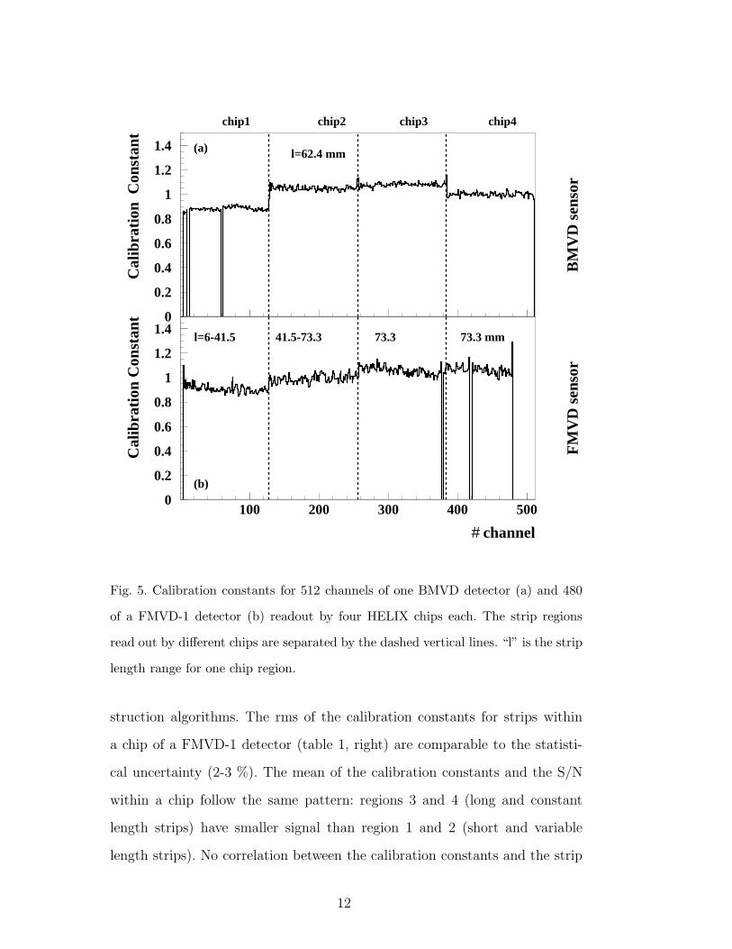
Fig. 5. Calibration constants for 512 channels of one BMVD detector (a) and 480

of a FMVD-1 detector (b) readout by four HELIX chips each. The strip regions

read out by different chips are separated by the dashed vertical lines. “l” is the strip

length range for one chip region.

struction algorithms. The rms of the calibration constants for strips within

a chip of a FMVD-1 detector (table 1, right) are comparable to the statisti-

cal uncertainty (2-3 %). The mean of the calibration constants and the S/N

within a chip follow the same pattern: regions 3 and 4 (long and constant

length strips) have smaller signal than region 1 and 2 (short and variable

length strips). No correlation between the calibration constants and the strip

12

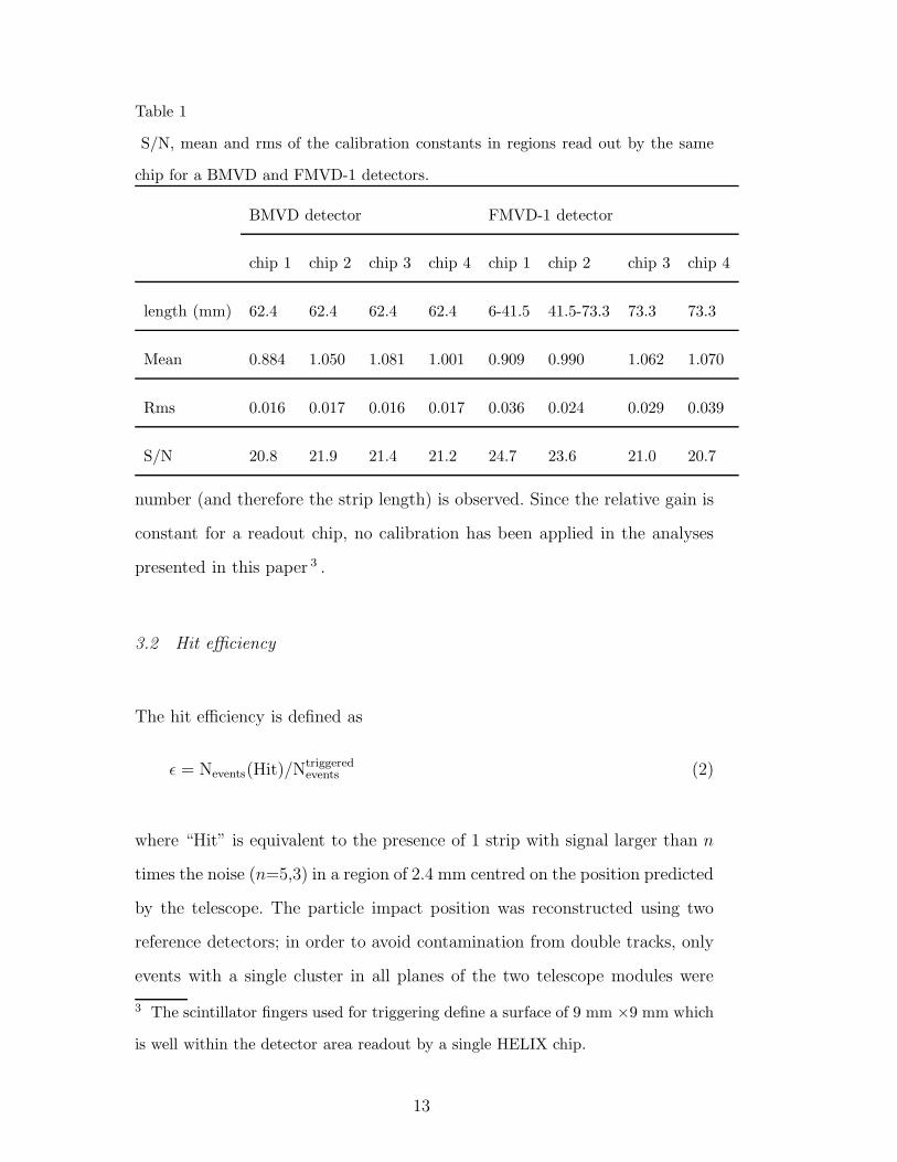
Table 1

S/N, mean and rms of the calibration constants in regions read out by the same

chip for a BMVD and FMVD-1 detectors.

BMVD detector FMVD-1 detector

chip 1 chip 2 chip 3 chip 4 chip 1 chip 2 chip 3 chip 4

length (mm) 62.4 62.4 62.4 62.4 6-41.5 41.5-73.3 73.3 73.3

Mean 0.884 1.050 1.081 1.001 0.909 0.990 1.062 1.070

Rms 0.016 0.017 0.016 0.017 0.036 0.024 0.029 0.039

S/N 20.8 21.9 21.4 21.2 24.7 23.6 21.0 20.7

number (and therefore the strip length) is observed. Since the relative gain is

constant for a readout chip, no calibration has been applied in the analyses

presented in this paper 3 .

3.2 Hit efficiency

The hit efficiency is defined as

ǫ = Nevents(Hit)/Ntriggeredevents (2)

where “Hit” is equivalent to the presence of 1 strip with signal larger than n

times the noise (n=5,3) in a region of 2.4 mm centred on the position predicted

by the telescope. The particle impact position was reconstructed using two

reference detectors; in order to avoid contamination from double tracks, only

events with a single cluster in all planes of the two telescope modules were

3 The scintillator fingers used for triggering define a surface of 9 mm ×9 mm which

is well within the detector area readout by a single HELIX chip.

13

accepted.

Using a sample of ∼ 105 events the 90% confidence limits on ǫ is 99.96% >

ǫ5 > 99.95% (99.997%) for a signal in the MVD detector larger than 5 (3)

times the noise.

3.3 Detector performance as a function of the bias voltage

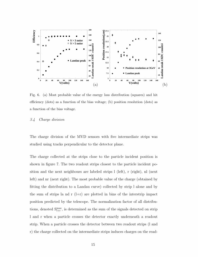
The dependence of the detector performance as a function of Vbias has been

investigated. Figure 6(a) shows the most probable value of the energy loss

distribution 4 and the hit efficiency as a function of the bias voltage. For

values of Vbias above the depletion voltage (Vdep ≃ 85V ) a plateau is reached.

The signal collection degrades with decreasing Vbias, whereas the hit efficiency

remains constant at Vbias well below the depletion voltage. Only for Vbias<∼ 40 V

ǫ starts to decline. The noise level remains constant (∼ 6 ADC counts) for

values of Vbias > 5V.

The charge division of the detector and the position resolution (see sections 3.4

and 5, respectively, for detailed explanations) were also studied as a function

of Vbias. Figure 6(b) shows the position resolution as a function of Vbias: a

stable behaviour above ∼ 40 V can be observed. The charge division of the

detector has also found to be unvaried above ∼ 40 V [22]. It is remarkable that

with ∼ 9 V of effective voltage in the detector, with only ∼ 30% of the bulk

depleted, a resolution of 25 µm is achieved. As a conclusion, the performance

of the detector seems to be rather stable well below depletion voltage.

4 The most probable value of the energy loss distribution is defined as the peak

value from a fit by a Landau function.

14

0

0.2

0.4

0.6

0.8

1

0 20 40 60 80 100 120 140 160

Eff

icie

ncy

S > 3 noiseS > 5 noise

20

40

60

80

100

120

140

160

180

200

V(volts)

Lan

dau

peak

(A

DC

cou

nts)

Landau peak

(a)

5

7.5

10

12.5

15

17.5

20

22.5

25

27.5

0 20 40 60 80 100 120 140 160

Pos

itio

n re

solu

tion

(µm

)

Position resolution at 3GeV

Landau peak20

40

60

80

100

120

140

V(volts)

Lan

dau

peak

(A

DC

cou

nts)

(b)

Fig. 6. (a) Most probable value of the energy loss distribution (squares) and hit

efficiency (dots) as a function of the bias voltage; (b) position resolution (dots) as

a function of the bias voltage.

3.4 Charge division

The charge division of the MVD sensors with five intermediate strips was

studied using tracks perpendicular to the detector plane.

The charge collected at the strips close to the particle incident position is

shown in figure 7. The two readout strips closest to the particle incident po-

sition and the next neighbours are labeled strips l (left), r (right), nl (next

left) and nr (next right). The most probable value of the charge (obtained by

fitting the distribution to a Landau curve) collected by strip l alone and by

the sum of strips la nd r (l+r) are plotted in bins of the interstrip impact

position predicted by the telescope. The normalization factor of all distribu-

tions, denoted Smaxl+r , is determined as the sum of the signals detected on strip

l and r when a particle crosses the detector exactly underneath a readout

strip. When a particle crosses the detector between two readout strips (l and

r) the charge collected on the intermediate strips induces charges on the read-

15

Predicted position (µm)

Col

lect

ed c

harg

e

strip nlnl+nrstrip l

l+r

0

0.2

0.4

0.6

0.8

1

0 20 40 60 80 100 120

Fig. 7. Sum of the charge collected by the left and right readout strips (sum l+r,

solid line), the charge collected by the left readout strip (strip l, triangles) falling

from the interstrip impact position x=0 µm to the interstrip impact position x=120

µm, charge collected by the next left neighbour of the left readout strip (strip nl,

dots) and sum of the charge collected by both the next-to-closest readout strips

(sum nl+nr, open squares).

out ones producing a dependence on the distance to the impact position with

large deviations from linearity near the readout strips. Due to capacitative

couplings between the strip implants, the fraction of charge collected by strip

r is not negligible (∼ 10% Smaxl+r ) even for the case of particles crossing the

detector exactly underneath the readout strip l (positions x=0 in figure 7)

and vice versa. The charge collected by the next left neighbour of the readout

16

strip l, nl, and the sum (nl+nr) of the signal collected by the two neighbours

to the closest readout strips l (nl) and r (nr) is also shown in figure 7. The

measurement demonstrates that a simple model considering only capacitances

to neighbouring strip implants resulting in charge collected only at the two

neighbour strips is not satisfactory. Moreover, the sum of the two signals col-

lected by strip l and r is not completely flat as a function of the interstrip

position, showing a dip (-19 % Smaxl+r ) when the particles cross the detector

in the central region between the two readout strips. This is mainly due to

charge losses to the backplane. Taking into account the charge sharing to the

next-to-closest readout strips, the effective charge loss to the backplane is of

the order of ∼ 16 % .

4 Simulation of the MVD detector response

Diffusion, ionisation fluctuations, noise and charge division were included in

the simulation program which is described in [24], and is based on [25]. Charge

is generated inside the detector along the particle’s path implementing ionisa-

tion fluctuations tuned to other measurements with silicon detectors [25]. The

charge drifts to the detector surface under the effect of the electric field; it is

then assumed to be collected by the closest strip implant [25].

Once the charges are collected on the strip implants they have to be transferred

to the readout strips. The capacitive network is more complicated than the

simple sketch in figure 1, since also capacitances to next to strip implants even

further apart are taken into account [26]. Charge transfer coefficients have been

determined from testbeam measurements. They give the fraction of charge

on a strip implant which is transferred to the surrounding readout strips.

To measure these coefficients only tracks crossing the detector within 5µm

17

Table 2

Charge fraction collected by the four readout strips surrounding the particle im-

pact position. Only particles crossing the detector (between strips l and r) directly

underneath strip implants are selected.

Charge transfer coefficient

Particle Position nl l r nr sum

#1: strip l 0.091 0.815 0.091 0.004 1.000

#2: 1st intermediate 0.082 0.655 0.158 0.021 0.916

#3: 2nd intermediate 0.076 0.486 0.256 0.041 0.859

#4: 3rd intermediate 0.058 0.363 0.363 0.058 0.842

#5: 4th intermediate 0.041 0.256 0.486 0.076 0.859

#6: 5th intermediate 0.021 0.158 0.655 0.082 0.916

#7: strip r 0.004 0.091 0.815 0.091 1.000

underneath strip implants were used. The strip implants are numbered from

#1 to #7, starting from the left readout strip from the impact position. The

charge collected (i.e. the most probable value of the energy loss distribution)

on the four surrounding readout strips, denoted as next left (nl), left (l),

right (r) and next right (nr), is measured for tracks in positions #1 to #7.

High statistics data samples have been used in order to achieve an accuracy

better than 1%. The collected charge reaches a maximum for positions #1

and #7; all coefficients are normalized to this value. The detector response is

assumed to be symmetric. In the simulation all charges collected on a strip

implant are transferred to the four surrounding readout strips using these

measured coefficients (fractions smaller than 0.4% were neglected). For every

readout channel an additional signal according to Gaussian distributed noise

18

was simulated. The width of the Gaussian was chosen in order to obtain the

same S/N as measured in the testbeam data.

Comparison between the results of the simulation program with the data mea-

surements is presented in section 7.2.

5 Position reconstruction for perpendicular tracks

5.1 The eta algorithm.

A standard method to reconstruct the impact position, proven to work at

small incidence angle, is the so called η algorithm [27], [28] . It consists of

a non-linear interpolation between the two neighbouring strips of the cluster

which have collected the highest signals (indicated in the following as Sright

and Sleft, respectively). For each event, the quantity η:

η =Sright

Sright + Sleft(3)

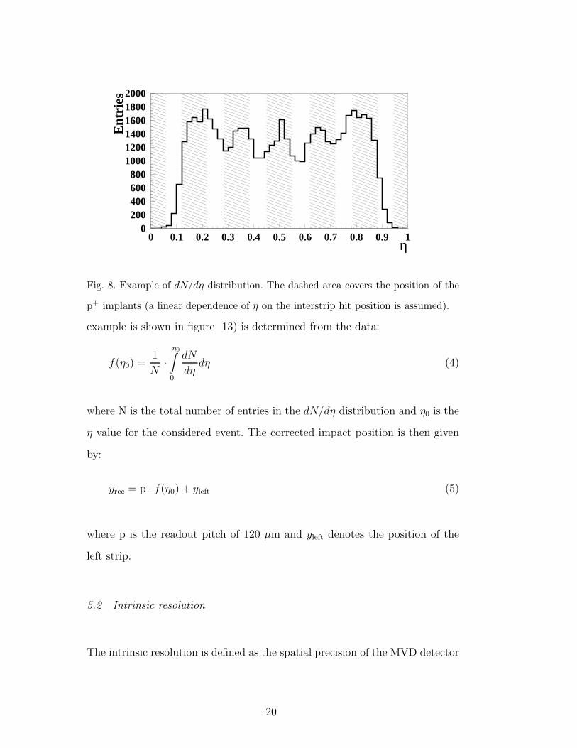
is calculated. Figure 8 shows the dN/dη distribution for the MVD detector

obtained from the testbeam data: in the region close to the readout strips there

are very few entries, and clear peaks can be seen elsewhere. In case of a fully

linear behaviour, the η distribution would be completely flat and the dashed

bands (where the peaks are observed) would represent the position of the

intermediate strips. The fact that the dN/dη is not uniform, although the beam

profile is uniform over the detector area, indicates that the capacitive charge

division mechanism is not fully linear in the hit position between readout

strips. To correct for this non-linearities a probability density function (an

19

0200400600800

100012001400160018002000

0 0.1 0.2 0.3 0.4 0.5 0.6 0.7 0.8 0.9 1η

Ent

ries

Fig. 8. Example of dN/dη distribution. The dashed area covers the position of the

p+ implants (a linear dependence of η on the interstrip hit position is assumed).

example is shown in figure 13) is determined from the data:

f(η0) =1

N·

η0∫

0

dN

dηdη (4)

where N is the total number of entries in the dN/dη distribution and η0 is the

η value for the considered event. The corrected impact position is then given

by:

yrec = p · f(η0) + yleft (5)

where p is the readout pitch of 120 µm and yleft denotes the position of the

left strip.

5.2 Intrinsic resolution

The intrinsic resolution is defined as the spatial precision of the MVD detector

20

Energy-2(GeV-2)

Pos

itio

n re

solu

tion

2 (µm

2 )

MVD Sensor

x/X0 = 0.0038 ± 0.0002

intr. Resol. = 7.2 ± 0.2 µm

6 5 4 3 2 Energy (GeV)

17.2

12.8

10.8

9.89.0

Pos

itio

n re

solu

tion

(µm

)

0

50

100

150

200

250

300

0 0.05 0.1 0.15 0.2 0.25 0.3

Fig. 9. Position resolution as a function of the beam energy. The result of the fit

for the ratio x/X0 (where x is the thickness of the material and X0 the radiation

length) is also shown.

The measured position resolution σres, defined as the width of the residual

distribution obtained from a fit to a Gaussian function, includes several con-

tributions:

σres =√

(σintrMVD)

2 + k · (σintrtele)

2 +∑

i

ki ·∆θ2ms (6)

where σintrMVD is the intrinsic resolution of the MVD detector, σintr

tele is the intrinsic

resolution of the telescope sensors, (k, ki) are geometrical factors [24] related to

the relative distances between the telescope modules, the MVD detector and

also including the thickness of the aluminium window foils, and∑

i ki ·∆θms

is the extrapolation error due to the multiple Coulomb scattering along the

particle direction, ∆θ2ms ∝ p−2beam [29].

21

To extract the intrinsic position resolution of the MVD detector (σintrMVD), the

contributions of the second (see subsection 2.1) and third term in equation

6 have been evaluated. The effect of the multiple Coulomb scattering at low

beam energy (2-6 GeV) cannot be neglected; the intrinsic resolution has been

extracted by fitting the residual distribution measured at several beam energies

(shown in figure 9) to the formula in equation 6. Since the production of δ-rays

can spoil the position resolution, (see subsection 7.4), a selection cut to reject

the events in the tail of the energy loss distribution has been applied in the

previous calculation:

Scluster ≤ 1.7 · Speak

where Scluster is the total cluster charge and Speak is the most probable energy

deposition. The intrinsic position resolution obtained for the MVD detector

at θ = 0 incidence angle is:

σintrMVD = 7.2± 0.2 µm

Different strip lengths do not affect significantly neither the resolution nor the

charge division mechanism [22].

5.3 Resolution vs interstrip hit position

Figure 10(a) shows the position resolution as a function of the interstrip hit

position. The presence of an alternate systematic pattern when moving from

a p+ implant to the next one is noticeable. However, the variations observed

are in general very small (<∼ 1µm). In the region close to the readout strips,

the position resolution becomes slightly worse. This effect is a consequence

of the use of only two readout strips for the position reconstruction: when

22

a particle traverses the silicon sensor very close to a readout strip, a high

signal is induced on that readout strip and only relatively small signals on

the neighbouring ones. Therefore the η algorithm becomes more sensitive to

noise fluctuations. Figure 10(b) shows the mean value of the Gaussian fit to

the residual distribution (corresponding to a systematic shift from the origin)

as a function of the interstrip hit position. Close to the readout strips the

systematic shift in the position reconstruction is larger (∼ 1.5-2 µm) than in

the central area between readout strips (<∼ 1 µm).

0

2

4

6

8

10

12

14

0 20 40 60 80 100 120

Interstrip position (µm)

Pos

itio

n re

solu

tion

(µm

)

(a)

-4

-3

-2

-1

0

1

2

3

4

0 20 40 60 80 100 120

Interstrip position (µm)

Mea

n va

lue

(µm

)

(b)

Fig. 10. (a) Position resolution and (b) average residual shift from the origin as

a function of the interstrip hit position. Note that in this case no cut to reject

δ-electrons has been applied. The hatched bands indicate the position of the readout

and intermediate strips.

23

6 Position reconstruction for small angle of incidence tracks

6.1 The 3-strips algorithm

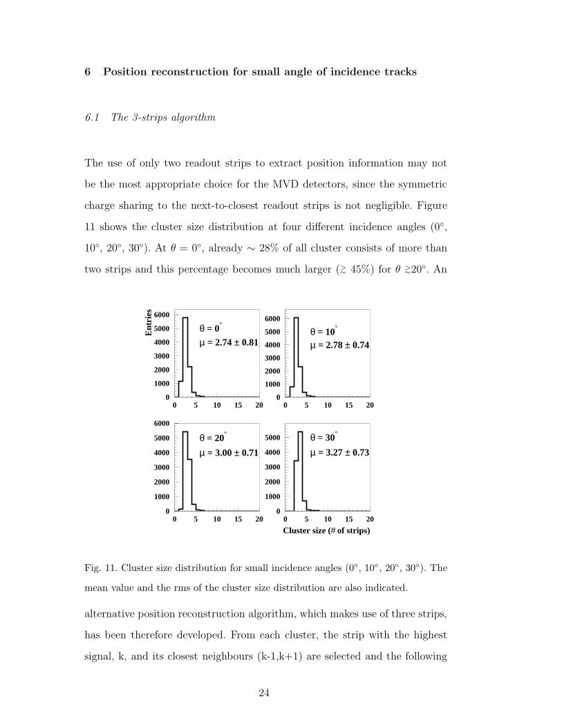
The use of only two readout strips to extract position information may not

be the most appropriate choice for the MVD detectors, since the symmetric

charge sharing to the next-to-closest readout strips is not negligible. Figure

11 shows the cluster size distribution at four different incidence angles (0,

10, 20, 30). At θ = 0, already ∼ 28% of all cluster consists of more than

two strips and this percentage becomes much larger (>∼ 45%) for θ >∼20

. An

0

1000

2000

3000

4000

5000

6000

0 5 10 15 20

Ent

ries

θ = 0°

µ = 2.74 ± 0.81

0

1000

2000

3000

4000

5000

6000

0 5 10 15 20

θ = 10°

µ = 2.78 ± 0.74

0

1000

2000

3000

4000

5000

6000

0 5 10 15 20

θ = 20°

µ = 3.00 ± 0.71

0

1000

2000

3000

4000

5000

0 5 10 15 20

θ = 30°

µ = 3.27 ± 0.73

Cluster size (# of strips)

Fig. 11. Cluster size distribution for small incidence angles (0, 10, 20, 30). The

mean value and the rms of the cluster size distribution are also indicated.

alternative position reconstruction algorithm, which makes use of three strips,

has been therefore developed. From each cluster, the strip with the highest

signal, k, and its closest neighbours (k-1,k+1) are selected and the following

24

quantities are calculated:

pleft =Sk · k + Sk−1 · (k − 1)

Sk + Sk−1and pright =

Sk · k + Sk+1 · (k + 1)

Sk + Sk+1(7)

The uncorrected reconstructed position prec (in analogy to the linear η inter-

polation) is then defined as:

prec =pleft · wn + pright

1 + wnwhere w = Sk−1/Sk+1 ; n = 2. (8)

n = 2 is found to work better than n = 1 because in the former case noise

is suppressed by giving less weigh to the strip with the lowest charge. The

corresponding interstrip position p is given by:

p = mod(prec, 1.)

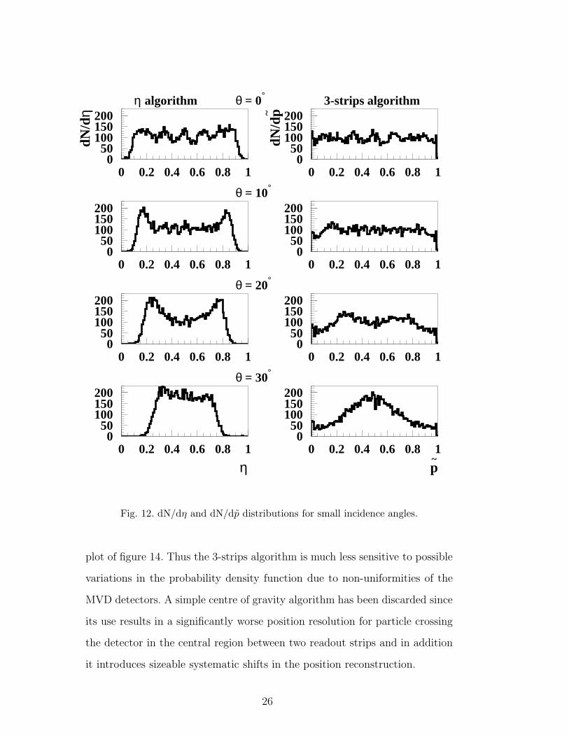
Figure 12 shows the dN/dη and dN/dp distributions for small incidence an-

gles (0, 10, 20, 30). By means of the 3-strips algorithm a more uniform

distribution can be obtained. In analogy with the η algorithm a probability

density function can be defined and the corrected impact position is given by:

yrec = p · f(p0) + p · pleft (9)

where p is the readout pitch and pleft denotes the position reconstructed using

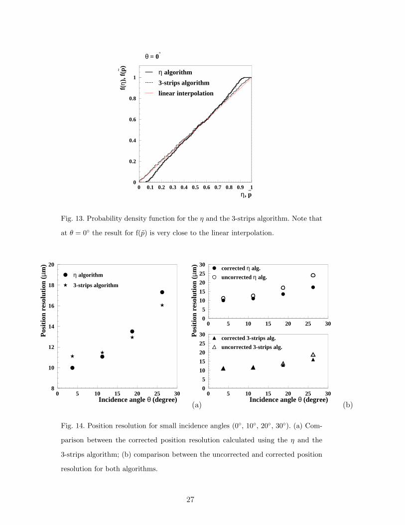
the left and the central strips. Figure 13 shows the comparison between f(p)

and f(η) for θ = 0. The position resolutions obtained using the η algorithm

and the 3-strips algorithm for the four different incidence angles (0, 10,

20, 30) are shown in figure 14. The resolution at 0 calculated with the 3-

strips algorithm is slightly worse than the one obtained with the η algorithm.

Nevertheless the non-linearity correction for the 3-strips algorithm is much

smaller than the one needed for the η algorithm up to 30, as shown in the right

25

050

100150200

0 0.2 0.4 0.6 0.8 1

η algorithm θ = 0°dN

/dη

050

100150200

0 0.2 0.4 0.6 0.8 1

3-strips algorithm

dN/d

p~0

50100150200

0 0.2 0.4 0.6 0.8 1

θ = 10°

050

100150200

0 0.2 0.4 0.6 0.8 1

050

100150200

0 0.2 0.4 0.6 0.8 1

θ = 20°

050

100150200

0 0.2 0.4 0.6 0.8 1

050

100150200

0 0.2 0.4 0.6 0.8 1

θ = 30°

η

050

100150200

0 0.2 0.4 0.6 0.8 1

p~

Fig. 12. dN/dη and dN/dp distributions for small incidence angles.

plot of figure 14. Thus the 3-strips algorithm is much less sensitive to possible

variations in the probability density function due to non-uniformities of the

MVD detectors. A simple centre of gravity algorithm has been discarded since

its use results in a significantly worse position resolution for particle crossing

the detector in the central region between two readout strips and in addition

it introduces sizeable systematic shifts in the position reconstruction.

26

0

0.2

0.4

0.6

0.8

1

0 0.1 0.2 0.3 0.4 0.5 0.6 0.7 0.8 0.9 1

η algorithm

3-strips algorithm

linear interpolation

η, p~

f(η)

, f(p~

)

θ = 0°

Fig. 13. Probability density function for the η and the 3-strips algorithm. Note that

at θ = 0 the result for f(p) is very close to the linear interpolation.

8

10

12

14

16

18

20

0 5 10 15 20 25 30

η algorithm

3-strips algorithm

Incidence angle θ (degree)

Pos

itio

n re

solu

tion

(µm

)

(a)

0

5

10

15

20

25

30

0 5 10 15 20 25 30

corrected η alg.

uncorrected η alg.

Pos

itio

n re

solu

tion

(µm

)

0

5

10

15

20

25

30

0 5 10 15 20 25 30Incidence angle θ (degree)

corrected 3-strips alg.

uncorrected 3-strips alg.

(b)

Fig. 14. Position resolution for small incidence angles (0, 10, 20, 30). (a) Com-

parison between the corrected position resolution calculated using the η and the

3-strips algorithm; (b) comparison between the uncorrected and corrected position

resolution for both algorithms.

27

6.2 Performance as a function of the φ angle

In the barrel section of the MVD the angle φ can be as large as 70. However

the size of the optical bench in the testbeam setup limited the measurement to

a maximum angle φ of 30. In the forward section of the MVD the φ range is

bigger than the θ range due to the orientation and position of the FMVD strips

with respect to the interaction point 5 . Although the maximum angle φ in the

FMVD is only ∼30, this is correlated with physical quantities of interest such

as the pseudorapidity of the track; any systematic effect could be thus relevant

for high momentum tracks as the one of the scattered electron at high Q2. In

the data analysis for the FMVD sensors, the width of the residual distribution

was ∼2-3 µm larger than in the standard setup (used for BMVD sensors)

because of the different geometrical constraints (i.e. the telescope modules

had to be moved away from the MVD sensor). The expected increase of the

signal with the path length inside the detector (∝ cos(φ)−1) was observed [22].

Figure 15(a) shows the position resolution as a function of the angle φ for

several beam energies. A rather flat behaviour is observed in the relevant range

for the FMVD. In figure 15(b) the squared position resolution as a function

of 1/E2 is shown for two different angles (0 and 30). The contribution of

multiple scattering shows up as a linear behaviour and the intrinsic resolution

corresponds to the intercept at the origin (i.e. for infinite momentum particles)

as it was discussed in subsection 5.2. The data at φ = 30 (squares) seem to

have a larger slope and a smaller intercept compared with the results for φ = 0

(dots). The larger slope can be attributed to the increase in the material of

5 This is true if the curvature induced by the magnetic field is not taken into

account. For low momenta particles the angle θ can be also large.

28

5

7.5

10

12.5

15

17.5

20

22.5

25

27.5

30

-5 0 5 10 15 20 25 30 35

Φ angle (degree)

Pos

itio

n re

solu

tion

(µm

)

6 GeV4 GeV3 GeV2 GeV

(a)

100

200

300

400

500

600

700

0 0.05 0.1 0.15 0.2 0.25 0.3

Energy-2 (GeV-2)P

osit

ion

reso

luti

on2 (

µm2 )

0 deg

30 deg

65 4 3 2 Energy (GeV)

12.5

18.4

14.4

11.1

Pos

itio

n re

solu

tion

(µm

)

(b)

Fig. 15. (a) Position resolution as a function of the angle φ; (b) σ2 as a function of

1/E2. A fit to the data at φ = 30 is also shown.

a factor cos(30)−1 ∼ 1.15. In addition, the larger S/N obtained at larger φ

angles can produce a better intrinsic resolution (as indicated by the smaller

intercept). Systematic effects have been evaluated to be smaller than 4%,

dominating over the statistical accuracy of ∼1.4%.

7 Position resolution for large angle of incidence tracks

At large incidence angles (θ > 30) the charge is spread over several strips and

the total cluster signal becomes larger as the particle’s path length increases:

S(θ) ∝S(θ = 0)

cos θ(10)

Since the central strips have on average the same signal, the information on

29

0

1000

2000

3000

4000

5000

6000

7000

0 5 10 15 20

Ent

ries θ = 40°

µ = 3.96 ± 0.79

0

1000

2000

3000

4000

5000

6000

7000

0 5 10 15 20

θ = 50°

µ = 4.70 ± 0.80

0

1000

2000

3000

4000

5000

6000

7000

0 5 10 15 20

θ = 60°

µ = 5.91 ± 0.83

0

1000

2000

3000

4000

5000

6000

7000

0 5 10 15 20

θ = 70°

µ = 8.33 ± 0.87

Cluster size (# of strips)

Fig. 16. Cluster size distributions for large incidence angles (40, 50, 60, 70)

the impact position is essentially contained only in the positions and signals of

the cluster edge strips. Therefore reconstruction algorithms such as the η one

are inadequate to calculate the particle impact point on the detector. Figure

16 shows the cluster size distributions for large angles of incidence (40, 50,

60, 70). Figure 17(a) shows the energy loss distribution for various incidence

angles (0, 30, 50, 60, 70), whereas the most probable value for the energy

deposition as a function of the incidence angle is shown in figure 17(b). In this

case the energy deposition is defined by summing up the signals measured on

± 5 strips around the predicted position:

Stot =+5∑

i=−5

Si

The result of a fit to the function:

f(θ, P1, P2) =P1

cos θP2

(11)

30

0

50

100

150

200

250

300

350

400

450

500

0 100 200 300 400 500 600 700 800 900

θ = 70°

θ = 60°

θ = 50°

θ = 30°

θ = 0°

Cluster pulse height (ADC counts)

Ent

ries

(a)

0

100

200

300

400

500

0 10 20 30 40 50 60 70

θ angle (degree)

Pea

k si

gnal

(A

DC

cou

nts)

P1 = 149.0 ± 4.0P2 = 1.09 ± 0.05

P2 = 1.00

(b)

Fig. 17. (a) Energy loss distribution at various incidence angles; (b) most probable

value for the energy deposition as a function of the incidence angle.

is also presented. The value P2 = 1.09± 0.05 is in agreement with the expec-

tation in equation 10 (i.e. P2 = 1.0).

7.1 The head-tail algorithm

A standard position reconstruction algorithm, proven to work at large inci-

dence angle, is the so called ‘head-tail’ algorithm [28, 30]. All the strips with:

Sstrip > 3 · σchip

where Sstrip is the strip signal and σchip is the average chip noise, are considered.

The first (head) and the last (tail) strips belonging to a cluster are selected

and the impact position is defined as:

yrec =yhead + ytail

2+ htcorr with htcorr =

Stail − Shead

2· < S >strips· p (12)

31

where yhead (ytail) is the position of the head (tail) strip, Shead (Stail) is the

corresponding signal, p is the strip pitch and < S > is the average strip signal

over the cluster.

The difference (Stail − Shead) in the correction factor htcorr is used to shift

the average position (yhead + ytail)/2 towards the tail (Stail − Shead > 0) or

head (Stail − Shead < 0) strip of the cluster, taking into account the rough

proportionality of the energy loss to the particle path in the detector.

7.2 Comparison with the simulation

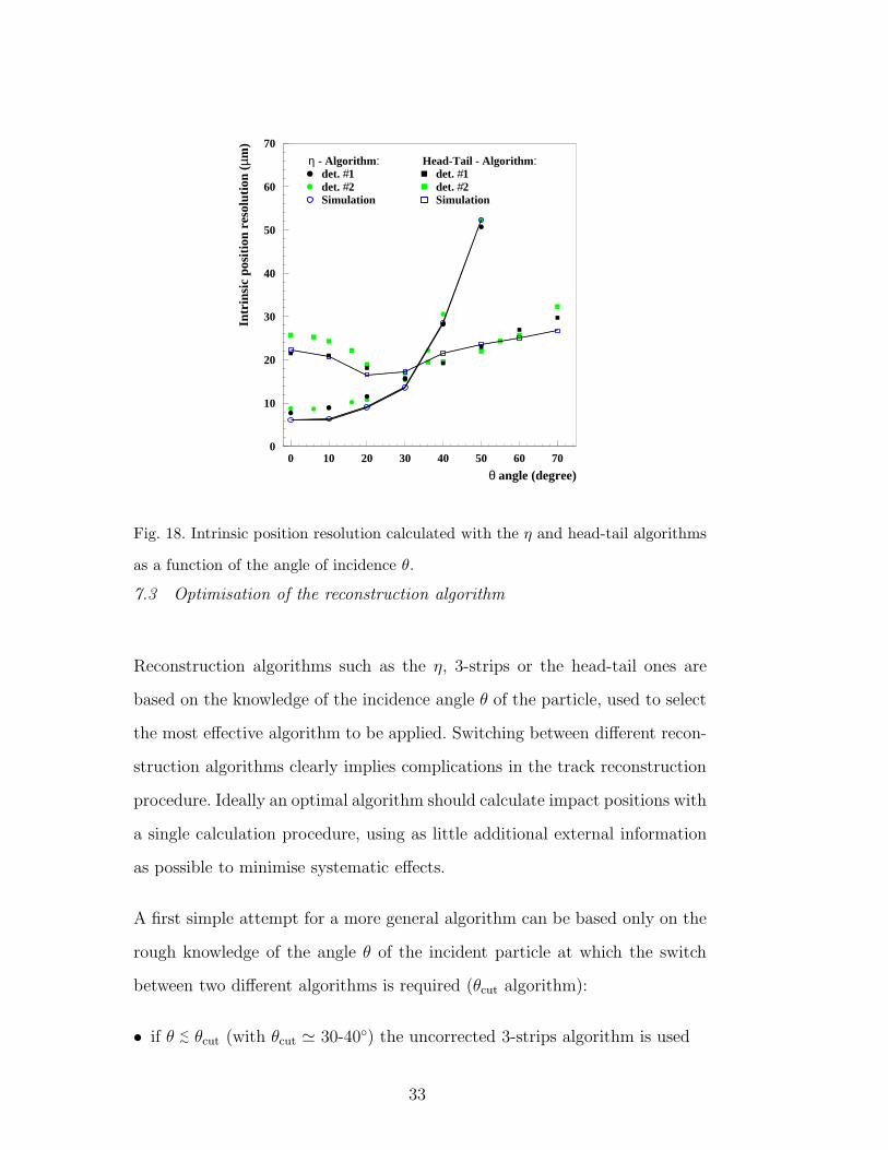
Figure 18 shows the position resolution calculated with the η and head-tail

algorithms as a function of the angle of incidence θ. At angles <∼ 30 the η

algorithm gives a much better resolution than the head-tail algorithm. How-

ever for angles >∼ 30-40, the latter proves to work much better. The results

using two different MVD barrel detectors are presented and compared with

the results obtained using the simulation program. The simulation is able to

describe the data over the whole angular region and for both reconstruction

algorithms. The S/N and charge transfer coefficients of det. #1 were used in

the simulation, which explains the slightly better agreement with this detec-

tor. Since δ-rays (see next section) are not taken into account the simulated

intrinsic resolution is found to be better than the one obtained from testbeam

data, especially for the η algorithm at small incident angles. The probability

that the two highest strips in the cluster, i.e. those used by the η algorithm,

are affected by a δ-ray which departs from the initial trajectory is smaller at

larger angles because the energy is deposited along more strips.

32

θ angle (degree)

Int

rins

ic p

osit

ion

reso

luti

on (

µm)

det. #1η - Algorithm:

det. #2Simulation

Head-Tail - Algorithm:det. #1det. #2Simulation

0

10

20

30

40

50

60

70

0 10 20 30 40 50 60 70

Fig. 18. Intrinsic position resolution calculated with the η and head-tail algorithms

as a function of the angle of incidence θ.

7.3 Optimisation of the reconstruction algorithm

Reconstruction algorithms such as the η, 3-strips or the head-tail ones are

based on the knowledge of the incidence angle θ of the particle, used to select

the most effective algorithm to be applied. Switching between different recon-

struction algorithms clearly implies complications in the track reconstruction

procedure. Ideally an optimal algorithm should calculate impact positions with

a single calculation procedure, using as little additional external information

as possible to minimise systematic effects.

A first simple attempt for a more general algorithm can be based only on the

rough knowledge of the angle θ of the incident particle at which the switch

between two different algorithms is required (θcut algorithm):

• if θ <∼ θcut (with θcut ≃ 30-40) the uncorrected 3-strips algorithm is used

33

0

10

20

30

40

50

60

0 10 20 30 40 50 60 70

θ angle (degree)

Pos

itio

n re

solu

tion

(µm

)

θcut alg. (det #1)θcut alg. (det #2)η alg.head-tail alg.

(a)

0

10

20

30

40

50

60

70

0 10 20 30 40 50 60 70

θ angle (degree)

Pos

itio

n re

solu

tion

(µm

)

cluster cut alg.η alghead-tail alg.

(b)

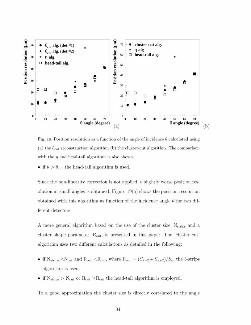
Fig. 19. Position resolution as a function of the angle of incidence θ calculated using

(a) the θcut reconstruction algorithm (b) the cluster-cut algorithm. The comparison

with the η and head-tail algorithm is also shown.

• if θ > θcut the head-tail algorithm is used.

Since the non-linearity correction is not applied, a slightly worse position res-

olution at small angles is obtained. Figure 19(a) shows the position resolution

obtained with this algorithm as function of the incidence angle θ for two dif-

ferent detectors.

A more general algorithm based on the use of the cluster size, Nstrips and a

cluster shape parameter, Rout, is presented in this paper. The ‘cluster cut’

algorithm uses two different calculations as detailed in the following:

• if Nstrips <Ncut and Rout <Rcut, where Rout = (Sk−2+Sk+2)/Sk, the 3-strips

algorithm is used.

• if Nstrips > Ncut or Rout ≥Rcut the head-tail algorithm is employed.

To a good approximation the cluster size is directly correlated to the angle

34

0250500750

1000

0 0.1 0.2 0.3 0.4 0.5 0.6 0.7 0.8 0.9 1E

ntri

es θ = 0°

0200400600800

0 0.1 0.2 0.3 0.4 0.5 0.6 0.7 0.8 0.9 1

θ = 30°

0100

200300400

0 0.1 0.2 0.3 0.4 0.5 0.6 0.7 0.8 0.9 1

θ = 50°

Rout

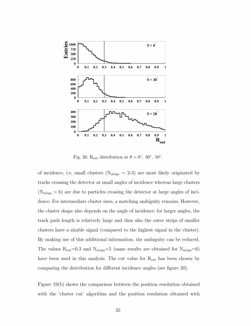
Fig. 20. Rout distribution at θ = 0, 30, 50.

of incidence, i.e. small clusters (Nstrips ∼ 2-3) are most likely originated by

tracks crossing the detector at small angles of incidence whereas large clusters

(Nstrips > 6) are due to particles crossing the detector at large angles of inci-

dence. For intermediate cluster sizes, a matching ambiguity remains. However,

the cluster shape also depends on the angle of incidence: for larger angles, the

track path length is relatively large and thus also the outer strips of smaller

clusters have a sizable signal (compared to the highest signal in the cluster).

By making use of this additional information, the ambiguity can be reduced.

The values Rcut=0.3 and Nstrips=5 (same results are obtained for Nstrips=6)

have been used in this analysis. The cut value for Rcut has been chosen by

comparing the distribution for different incidence angles (see figure 20).

Figure 19(b) shows the comparison between the position resolution obtained

with the ’cluster cut’ algorithm and the position resolution obtained with

35

the η and the head-tail algorithms. The position resolution achieved with

the uncorrected ‘cluster-cut’ algorithm is only slightly worse than the one

calculated with the best standard reconstruction method for each angle (i.e.

η and ‘head-tail’). Since the ‘cluster-cut’ algorithm does not need any angular

information, it could be a valuable choice for a first position reconstruction in

a general track reconstruction procedure.

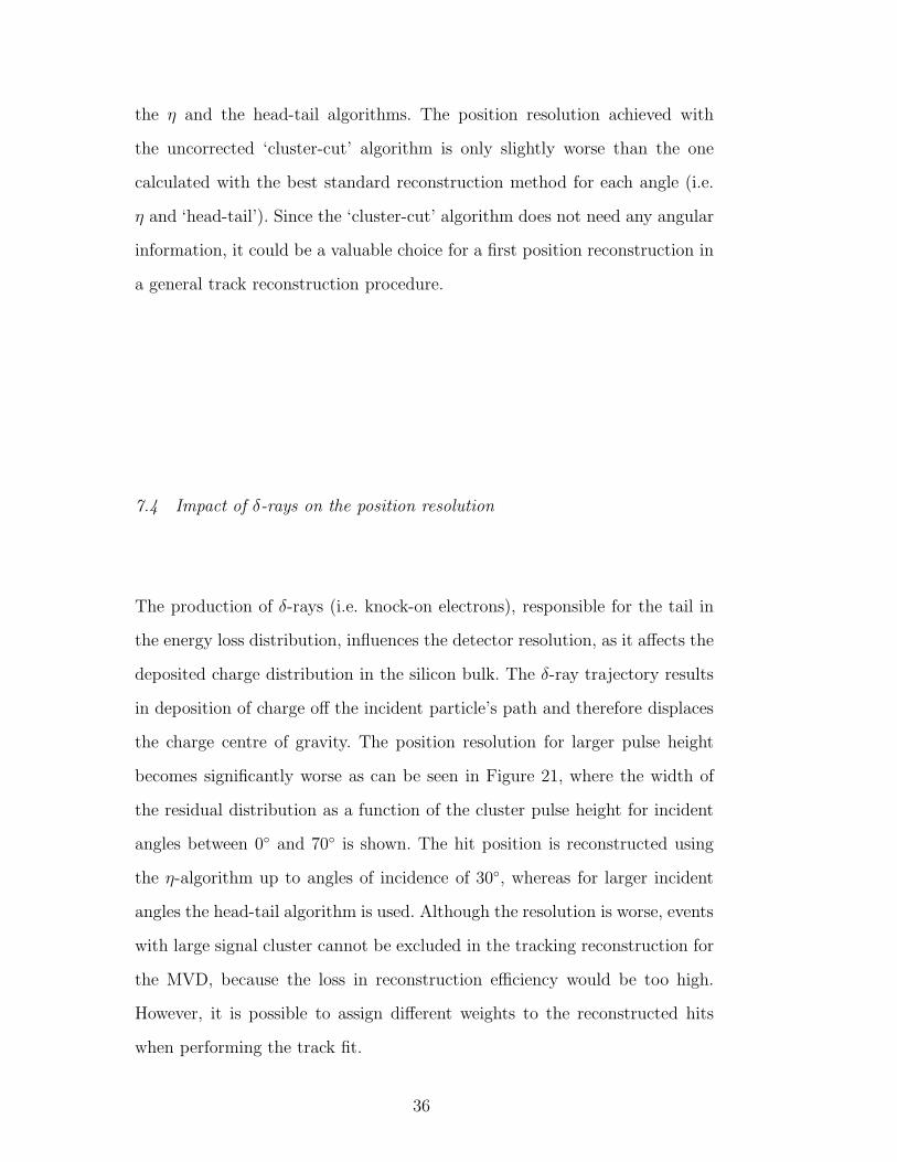
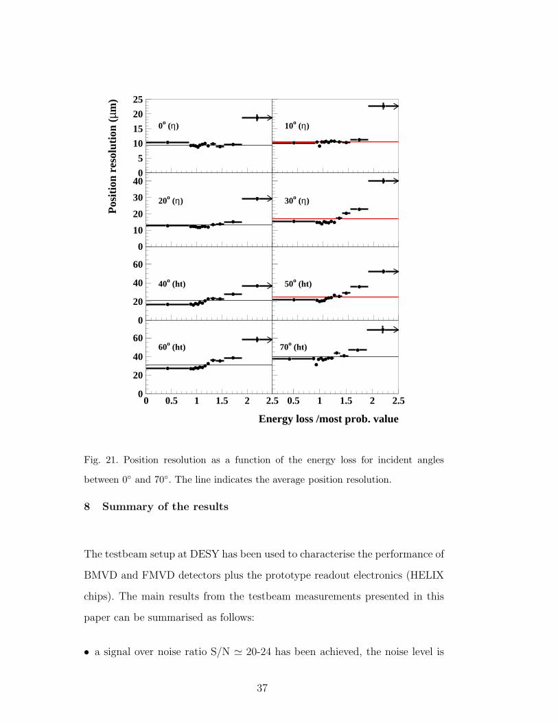
7.4 Impact of δ-rays on the position resolution

The production of δ-rays (i.e. knock-on electrons), responsible for the tail in

the energy loss distribution, influences the detector resolution, as it affects the

deposited charge distribution in the silicon bulk. The δ-ray trajectory results

in deposition of charge off the incident particle’s path and therefore displaces

the charge centre of gravity. The position resolution for larger pulse height

becomes significantly worse as can be seen in Figure 21, where the width of

the residual distribution as a function of the cluster pulse height for incident

angles between 0 and 70 is shown. The hit position is reconstructed using

the η-algorithm up to angles of incidence of 30, whereas for larger incident

angles the head-tail algorithm is used. Although the resolution is worse, events

with large signal cluster cannot be excluded in the tracking reconstruction for

the MVD, because the loss in reconstruction efficiency would be too high.

However, it is possible to assign different weights to the reconstructed hits

when performing the track fit.

36

0o (η)

Pos

itio

n re

solu

tion

(µm

) 10o (η)

20o (η) 30o (η)

40o (ht) 50o (ht)

60o (ht) 70o (ht)

Energy loss /most prob. value

0

5

10

15

20

25

0

10

20

30

40

0

20

40

60

0

20

40

60

0 0.5 1 1.5 2 2.5 0.5 1 1.5 2 2.5

Fig. 21. Position resolution as a function of the energy loss for incident angles

between 0 and 70. The line indicates the average position resolution.

8 Summary of the results

The testbeam setup at DESY has been used to characterise the performance of

BMVD and FMVD detectors plus the prototype readout electronics (HELIX

chips). The main results from the testbeam measurements presented in this

paper can be summarised as follows:

• a signal over noise ratio S/N ≃ 20-24 has been achieved, the noise level is

37

uniformly distributed over the strips;

• the detector efficiency ǫ is very high (> 99.95%);

• the calibration shows that gain variations of a single HELIX readout chip are

of the order of 2% and do not influence the position reconstruction algorithm

even in the case of detectors with strips of different lengths (FMVD);

• the charge division has been studied in detail. The expected charge sharing

between strip implants has been confirmed;

• the charge transfer between strip implants and readout strips has been pa-

rameterised and implemented in a detector simulation program which gives

a good description of the data;

• the intrinsic position resolution at normal angle of incidence σintrMVD = 7.2±

0.2 µm is highly satisfactory if compared to the value p/√12 ≃ 35µm which

represents the limit for a digital system with a readout pitch p = 120 µm;

• the position resolution is not strongly dependent on the angle φ in the range

of interest for the FMVD;

• the position resolution at large angle of incidence θ is still very satisfactory

(<∼ 40 µm up to θ = 70);

• a position reconstruction algorithm which uses the rough knowledge of the

angle of incidence θ to choose the most effective reconstruction procedure

has been developed. For small incidence angles a 3-strips algorithm is ap-

plied whereas for large incidence angles the head-tail algorithm is used;

• a general position reconstruction algorithm, not using prior knowledge of

the angle of incidence, has proven to work well up to θ = 70 and could

therefore be a valuable choice for a first position reconstruction in the track

reconstruction procedure;

• the production of δ-rays causes a deterioration of the position resolution.

Since events with very large cluster signal cannot be excluded from the MVD

data, the hit positions used for a track fit should be weighted according to

38

their pulse height.

References

[1] U. Schneekloth (editor), “The HERA Luminosity Upgrade”, DESY internal

report, DESY-HERA 98-05, 1998.

[2] ZEUS Collaboration, M. Derrick et al., The ZEUS Detector, Status Report

1993, DESY, 1993.

[3] A. Garfagnini, Nucl. Instrum. Methods A 435, 1999 (34).

[4] R. Klanner, “The ZEUS Micro Vertex Detector”, proceedings of the

International Europhysics Conference on High Energy Physics, EPS-HEP 99,

Tampere, Finland.

[5] E. Koffeman, Nucl. Instrum. Methods A 453, 2000 (89).

[6] C. Coldewey, Nucl. Instrum. Methods A 453, 2000 (149).

[7] M. Feuerstack-Raible, U. Trunk, et al, “HELIX 128-x User’s Manual Version

2.1, 3.2.1999 ”, HD-ASIC-33-0697. Available at

http://wwwasic.kip.uni-heidelberg.de/~trunk/projects/Helix/.

[8] M. Feuerstack-Raible, Nucl. Instrum. Methods A 447, 2000 (35).

[9] M. C. Petruccci, Int. J. Mod. Phys. A Vol. 16 Suppl. 1C (2001) 1078,

[10] E. Koffeman, Nucl. Instrum. Methods A 473, 2001 (26).

[11] V. Chiochia, “The ZEUS Micro Vertex Detector”, proceedings of the Vertex

2002 conference, hep-ex/0111061, submitted to Nucl. Instrum. Methods A.

[12] C. Coldewey, Nucl. Instrum. Methods A 447, 2000 (44).

[13] A. Garfagnini and U. Kotz, Nucl. Instrum. Methods A 461, 2001 (158).

39

[14] D. Dannheim et al., Design and Tests of the Silicon Sensors for the ZEUS Micro

Vertex Detector, submitted for publication to Nucl. Instrum. Methods A.

[15] U. Kotz, Nucl. Instrum. Methods A 461, 2000 (210).

[16] LabView, product of National Instruments.

[17] C. Colledani et al., Nucl. Instrum. Methods A 372, 1996 (379).

[18] J.Straver et al., Nucl. Instrum. Methods A 348, 1994 (485).

[19] M. Milite, PhD Thesis, DESY-THESIS-2001-050. Available at

http://www-library.desy.de/cgi-bin/showprep.pl?desy-thesis-01-050.

[20] ICI Films, High Performance Films Group, Wilmington, Delaware 19897, USA.

[21] CERN EST/SM-CI, Photomechanical Technologies Workshop.

[22] I. Redondo, PhD Thesis, DESY-THESIS-2001-037. Available at

http://www-library.desy.de/cgi-bin/showprep.pl?desy-thesis-01-037.

[23] Internal communication on test of the F/E chips (unpublished). Available at

http://zeus.pd.infn.it/MVD/MVD.html.

[24] M. Moritz, PhD Thesis, DESY-THESIS-2002-009. Available at

http://www-library.desy.de/cgi-bin/showprep.pl?desy-thesis-02-009

[25] G. Bashindzhagyan and N. Korotkova, Simulation of Silicon Microstrip

Detector Resolution for ZEUS Vertex Upgrade, internal ZEUS note, 99-023,

Hamburg (Germany), (1999).

[26] J. Martens, Simulationen und Qualitatssicherung der Siliziumstreifendetektoren

des ZEUS-Mikrovertexdetektors, DESY-THESIS-1999-044, Diplomarbeit,

University of Hamburg (1999).

[27] E. Belau et al., Nucl. Instrum. Methods 214, 1983 (253).

40

[28] R. Turchetta, Nucl. Instrum. Methods A 335, 1993 (44).

[29] D.E. Groom et al., The European Physical Journal C15 (2000) 1.

[30] KEK Preprint 96-172, Measurement of the Spatial Resolution of Wide-pitch

Silicon Strip Detectors with Large Incident Angle.

41