Embed Size (px)
DESCRIPTION
Analysing the natural frequency of system is fundamental for structural and acoustic design in order to predict and understand system’s dynamic behaviour.
Citation preview

1
VIA University College
Mechanical Engineering
Programme
Dorin Bordeasu (164631)
Khem Raj Guatam (164645)
Javier Camacho (164649)
Beam Modal Analysis
Spring 2013 Beam Modal Analysis Page 2
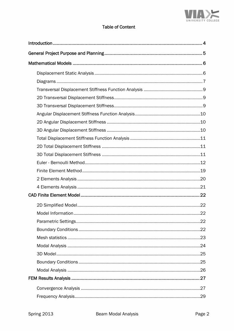
Table of Content
Introduction ................................................................................................................. 4
General Project Purpose and Planning .......................................................................... 5
Mathematical Models .................................................................................................. 6
Displacement Static Analysis ........................................................................................ 6
Diagrams ....................................................................................................................... 7
Transversal Displacement Stiffness Function Analysis ................................................ 9
2D Transversal Displacement Stiffness ........................................................................ 9
3D Transversal Displacement Stiffness ........................................................................ 9
Angular Displacement Stiffness Function Analysis .....................................................10
2D Angular Displacement Stiffness ............................................................................10
3D Angular Displacement Stiffness ............................................................................10
Total Displacement Stiffness Function Analysis .........................................................11
2D Total Displacement Stiffness ................................................................................11
3D Total Displacement Stiffness ................................................................................11
Euler - Bernoulli Method..............................................................................................12
Finite Element Method ................................................................................................19
2 Elements Analysis ....................................................................................................20
4 Elements Analysis ....................................................................................................21
CAD Finite Element Model .......................................................................................... 22
2D Simplified Model ....................................................................................................22
Model Information .......................................................................................................22
Parametric Settings .....................................................................................................22
Boundary Conditions ...................................................................................................22
Mesh statistics ............................................................................................................23
Modal Analysis ............................................................................................................24
3D Model .....................................................................................................................25
Boundary Conditions ...................................................................................................25
Modal Analysis ............................................................................................................26
FEM Results Analysis ................................................................................................. 27
Convergence Analysis .................................................................................................27
Frequency Analysis ......................................................................................................29
Spring 2013 Beam Modal Analysis Page 3
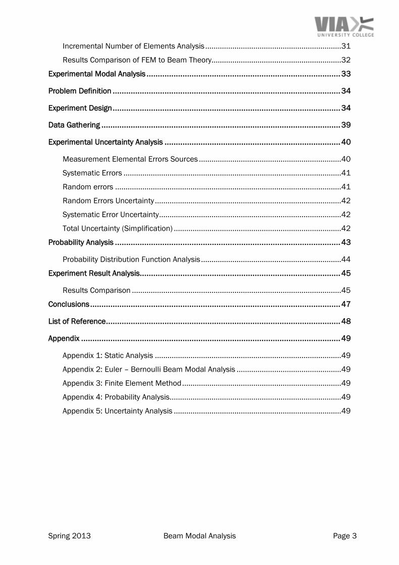
Incremental Number of Elements Analysis .................................................................31
Results Comparison of FEM to Beam Theory..............................................................32
Experimental Modal Analysis ...................................................................................... 33
Problem Definition ..................................................................................................... 34
Experiment Design ..................................................................................................... 34
Data Gathering .......................................................................................................... 39
Experimental Uncertainty Analysis .............................................................................. 40
Measurement Elemental Errors Sources ....................................................................40
Systematic Errors ........................................................................................................41
Random errors ............................................................................................................41
Random Errors Uncertainty .........................................................................................42
Systematic Error Uncertainty.......................................................................................42
Total Uncertainty (Simplification) ................................................................................42
Probability Analysis .................................................................................................... 43
Probability Distribution Function Analysis ...................................................................44
Experiment Result Analysis......................................................................................... 45
Results Comparison ....................................................................................................45
Conclusions ............................................................................................................... 47
List of Reference ........................................................................................................ 48
Appendix ................................................................................................................... 49
Appendix 1: Static Analysis .........................................................................................49
Appendix 2: Euler – Bernoulli Beam Modal Analysis ..................................................49
Appendix 3: Finite Element Method ............................................................................49
Appendix 4: Probability Analysis..................................................................................49
Appendix 5: Uncertainty Analysis ................................................................................49

Spring 2013 Beam Modal Analysis Page 4
Introduction
Analysing the natural frequency of system is fundamental for structural and acoustic
design in order to predict and understand system’s dynamic behaviour.
All objects can be regarded as spring. When small external forces try to disturb them they
will try to get back to its original position because of stiffness of spring. When external
forces act, spring will tend to come to same position and when this process repeats
vibration is created. Vibration thus created is very small and cannot be detected easily.
As the disturbing frequency becomes larger the mass effect of system will oppose motion.
In order for system to vibrate external forces should be very big to overcome inertia of
mass to make rapid changes in direction of motion. In this case effect of stiffness of spring
is so small it becomes negligible.
As explained above, we can easily see system has two different region of behaviour. First
when small external forces are acted spring stiffness tries to keep the mass at equilibrium
position and system is stiffness controlled. In other words spring stiffness will basically act
as inward force as it will try to restore mass to base position.
And in second region of behaviour, when system is mass controlled, the inertia of mass will
try to keep the mass in same direction opposing rapid change of motion in extreme end of
each stroke. Thus mass effect can be explained as outward one.
Stiffness effect is independent of disturbing frequency but mass effect for given amplitude
is square function of frequency. So when frequency starts increasing from zero at certain
frequency stiffness effect and mass effect cancels out. At that point neither factor
restrains movement of mass. So system goes wild and vibrates maximum without control.
The frequency at which this behaviour occurs is called natural Frequency of a system.
As a course work for FEM and EEX natural frequency of beam structure were calculated
with different approaches and result were analysed. For simplicity, natural frequency of a
clamped-clamped circular bar made out of structural steel was the subject for experiment.
Spring 2013 Beam Modal Analysis Page 5
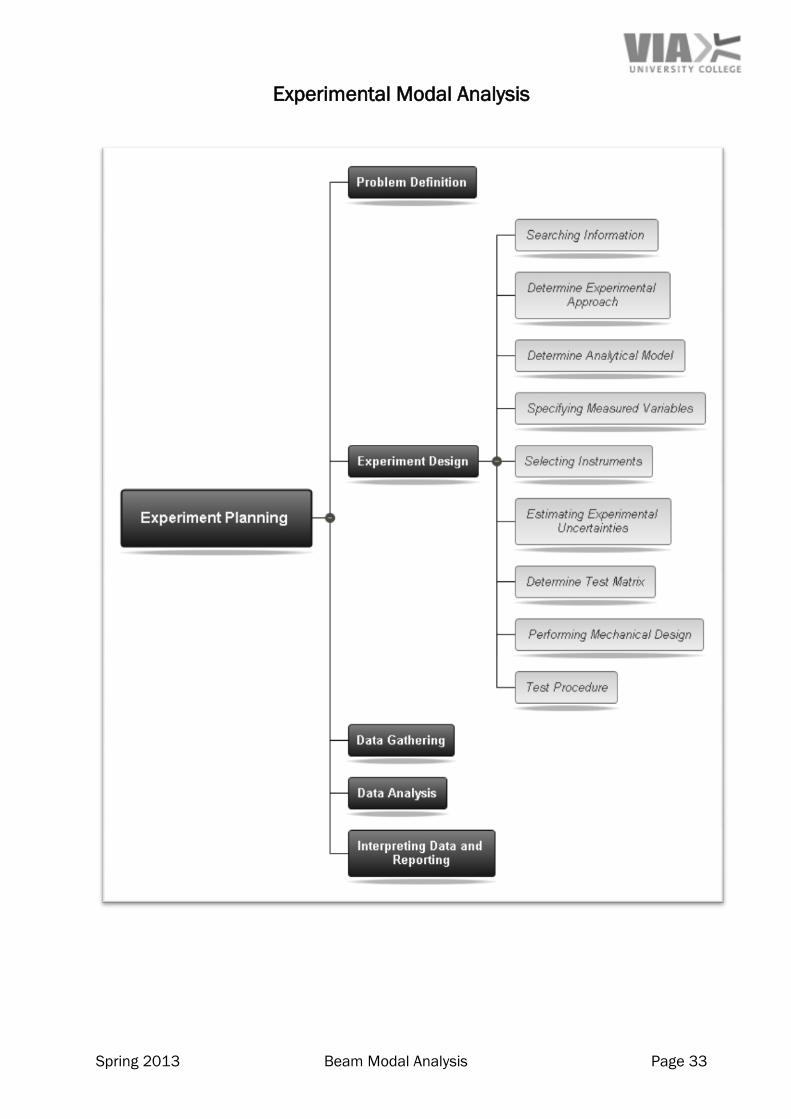
General Project Purpose and Planning
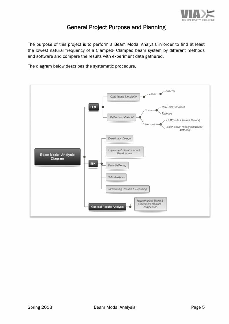
The purpose of this project is to perform a Beam Modal Analysis in order to find at least
the lowest natural frequency of a Clamped- Clamped beam system by different methods
and software and compare the results with experiment data gathered.
The diagram below describes the systematic procedure.
Spring 2013 Beam Modal Analysis Page 6
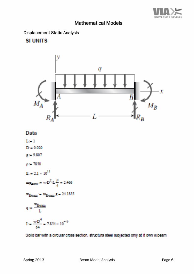
Mathematical Models
Displacement Static Analysis
Spring 2013 Beam Modal Analysis Page 7
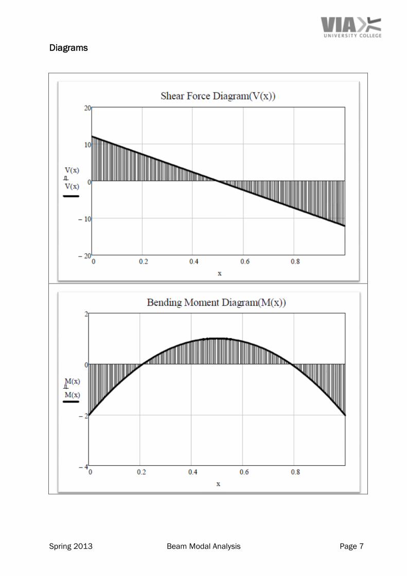
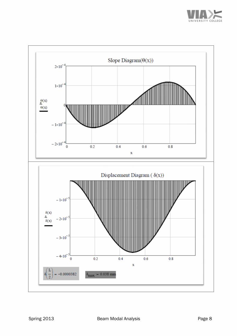
Diagrams
Spring 2013 Beam Modal Analysis Page 8
Spring 2013 Beam Modal Analysis Page 9
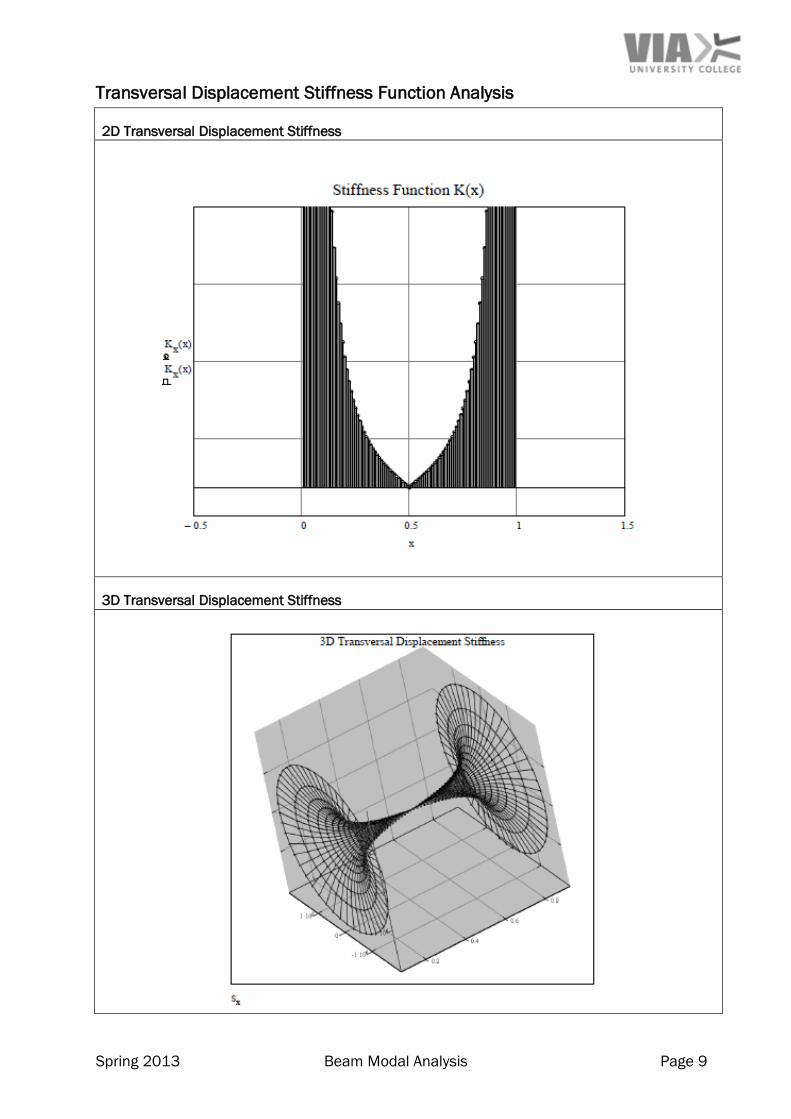
Transversal Displacement Stiffness Function Analysis
2D Transversal Displacement Stiffness
3D Transversal Displacement Stiffness
Spring 2013 Beam Modal Analysis Page 10
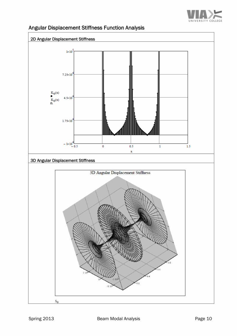
Angular Displacement Stiffness Function Analysis
2D Angular Displacement Stiffness
3D Angular Displacement Stiffness
Spring 2013 Beam Modal Analysis Page 11
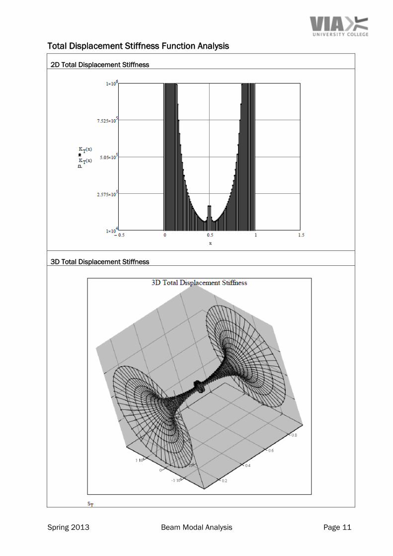
Total Displacement Stiffness Function Analysis
2D Total Displacement Stiffness
3D Total Displacement Stiffness
Spring 2013 Beam Modal Analysis Page 12
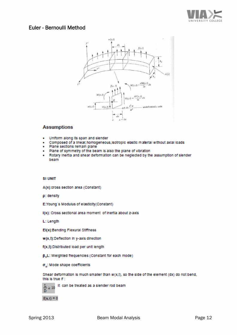
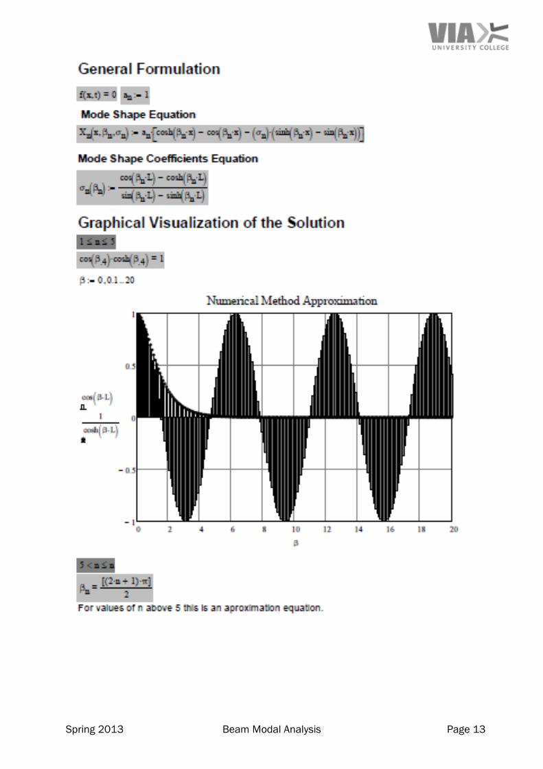
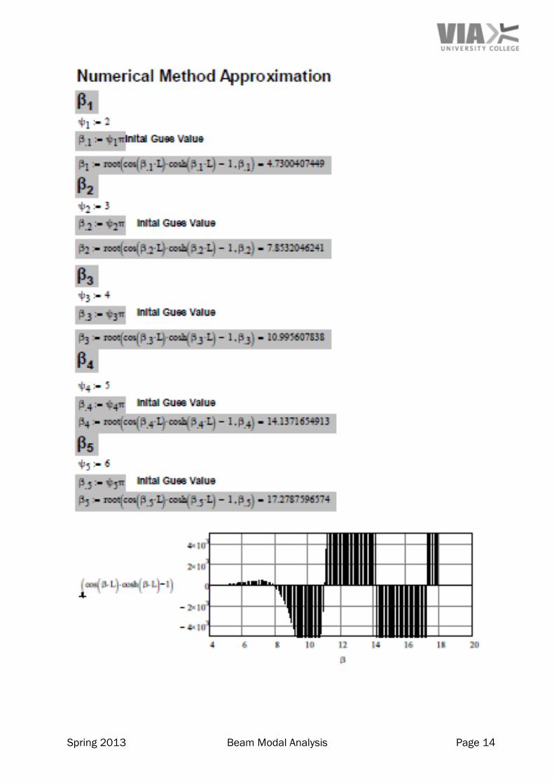
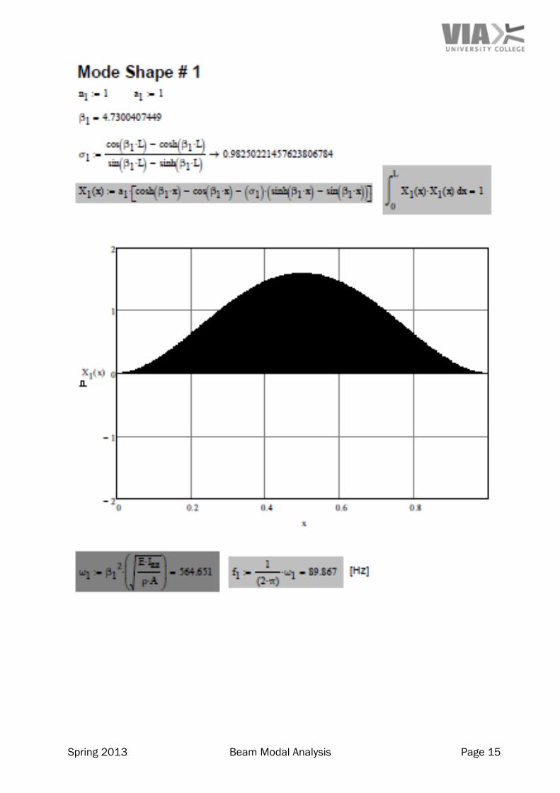
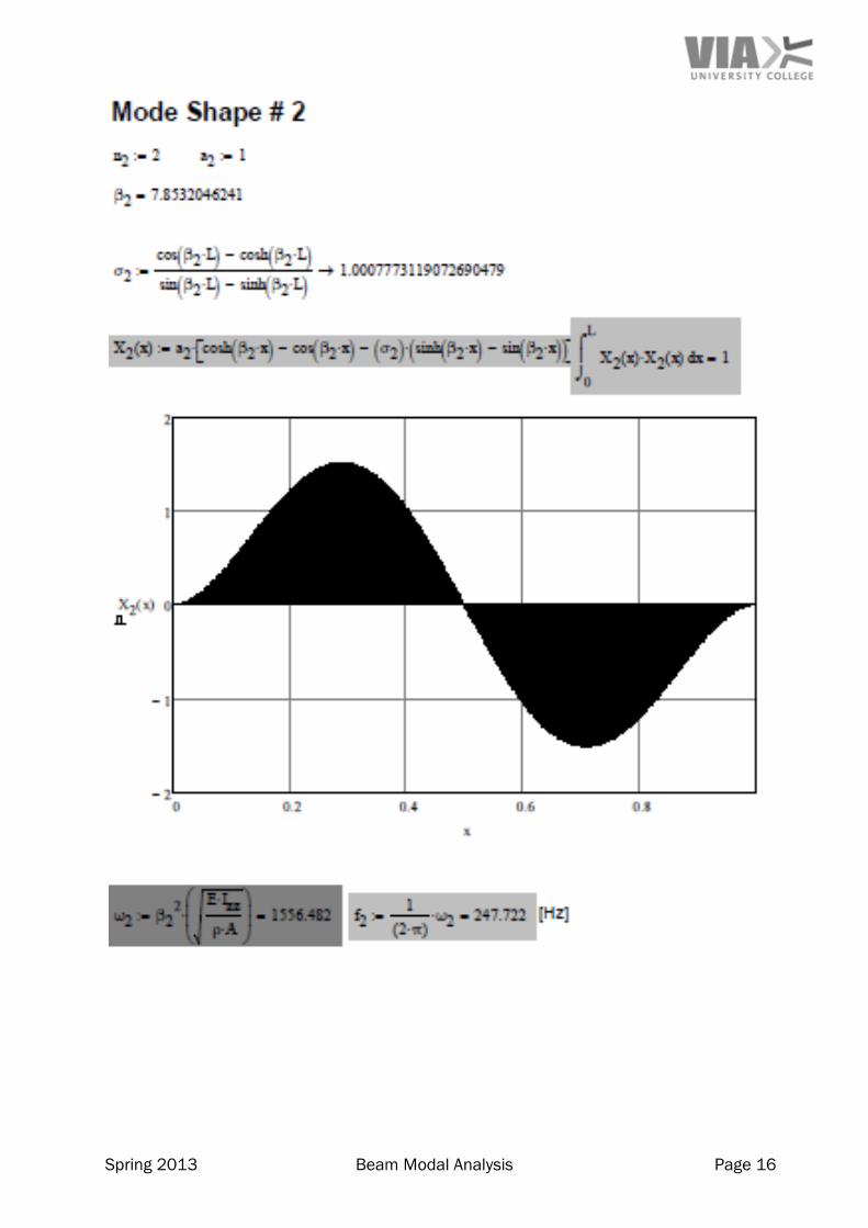
Euler - Bernoulli Method
Spring 2013 Beam Modal Analysis Page 13
Spring 2013 Beam Modal Analysis Page 14
Spring 2013 Beam Modal Analysis Page 15
Spring 2013 Beam Modal Analysis Page 16
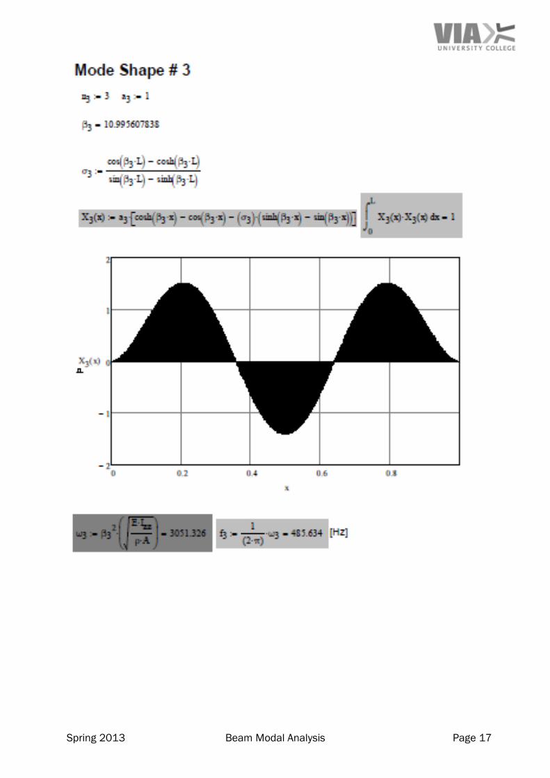
Spring 2013 Beam Modal Analysis Page 17
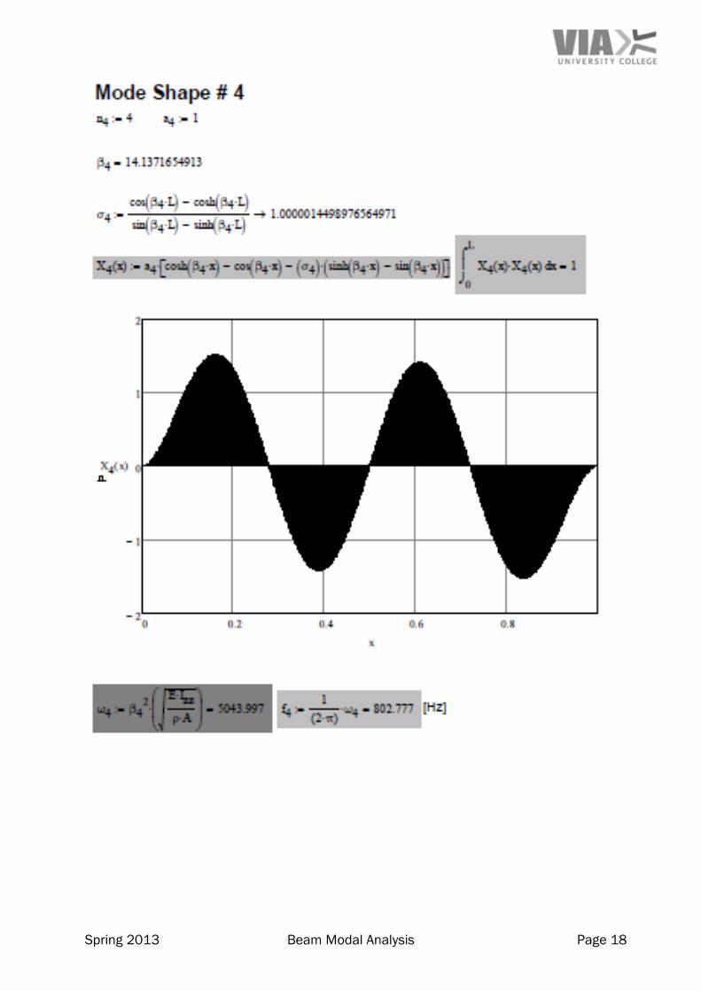
Spring 2013 Beam Modal Analysis Page 18
Spring 2013 Beam Modal Analysis Page 19
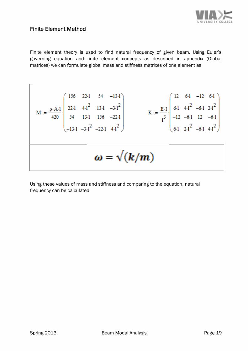
Finite Element Method
Finite element theory is used to find natural frequency of given beam. Using Euler’s
governing equation and finite element concepts as described in appendix (Global
matrices) we can formulate global mass and stiffness matrixes of one element as
Using these values of mass and stiffness and comparing to the equation, natural
frequency can be calculated.
Spring 2013 Beam Modal Analysis Page 20
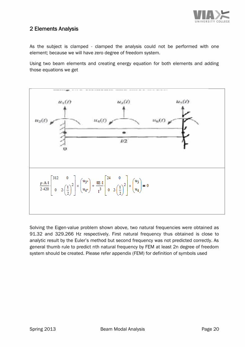
2 Elements Analysis
As the subject is clamped - clamped the analysis could not be performed with one
element; because we will have zero degree of freedom system.
Using two beam elements and creating energy equation for both elements and adding
those equations we get
Solving the Eigen-value problem shown above, two natural frequencies were obtained as
91.32 and 329.266 Hz respectively. First natural frequency thus obtained is close to
analytic result by the Euler’s method but second frequency was not predicted correctly. As
general thumb rule to predict nth natural frequency by FEM at least 2n degree of freedom
system should be created. Please refer appendix (FEM) for definition of symbols used
Spring 2013 Beam Modal Analysis Page 21
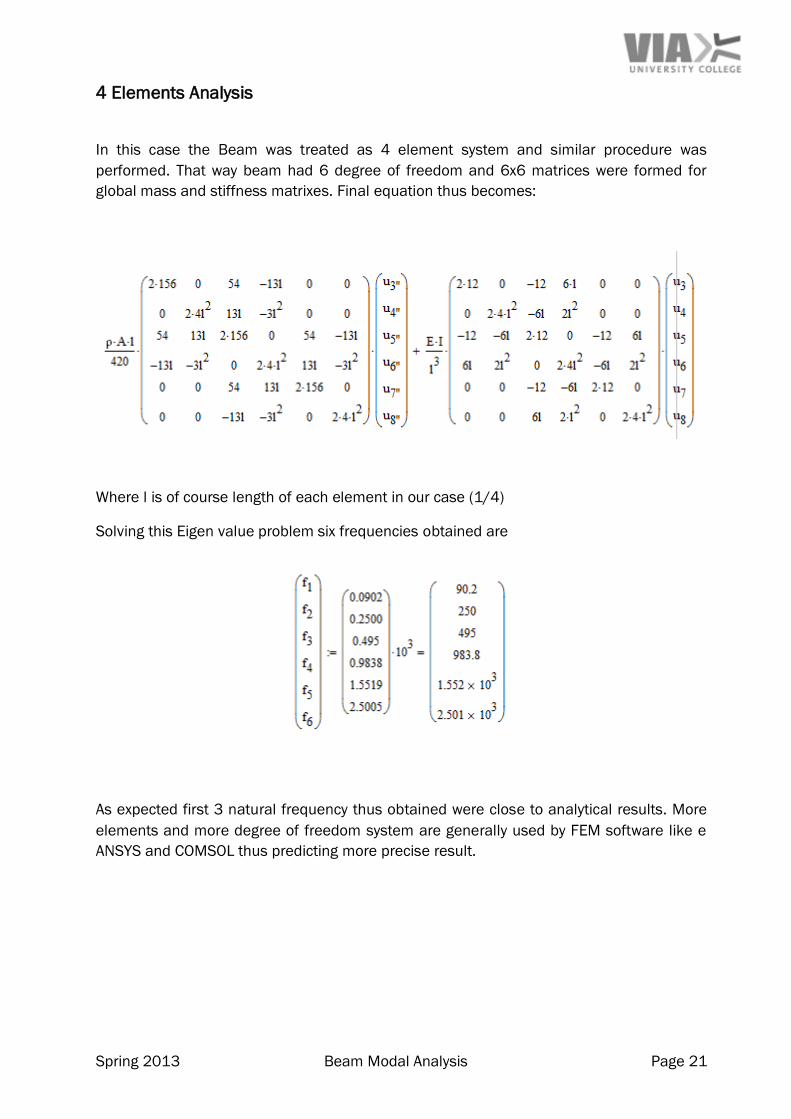
4 Elements Analysis
In this case the Beam was treated as 4 element system and similar procedure was
performed. That way beam had 6 degree of freedom and 6x6 matrices were formed for
global mass and stiffness matrixes. Final equation thus becomes:
Where l is of course length of each element in our case (1/4)
Solving this Eigen value problem six frequencies obtained are
As expected first 3 natural frequency thus obtained were close to analytical results. More
elements and more degree of freedom system are generally used by FEM software like e
ANSYS and COMSOL thus predicting more precise result.
Spring 2013 Beam Modal Analysis Page 22
CAD Finite Element Model
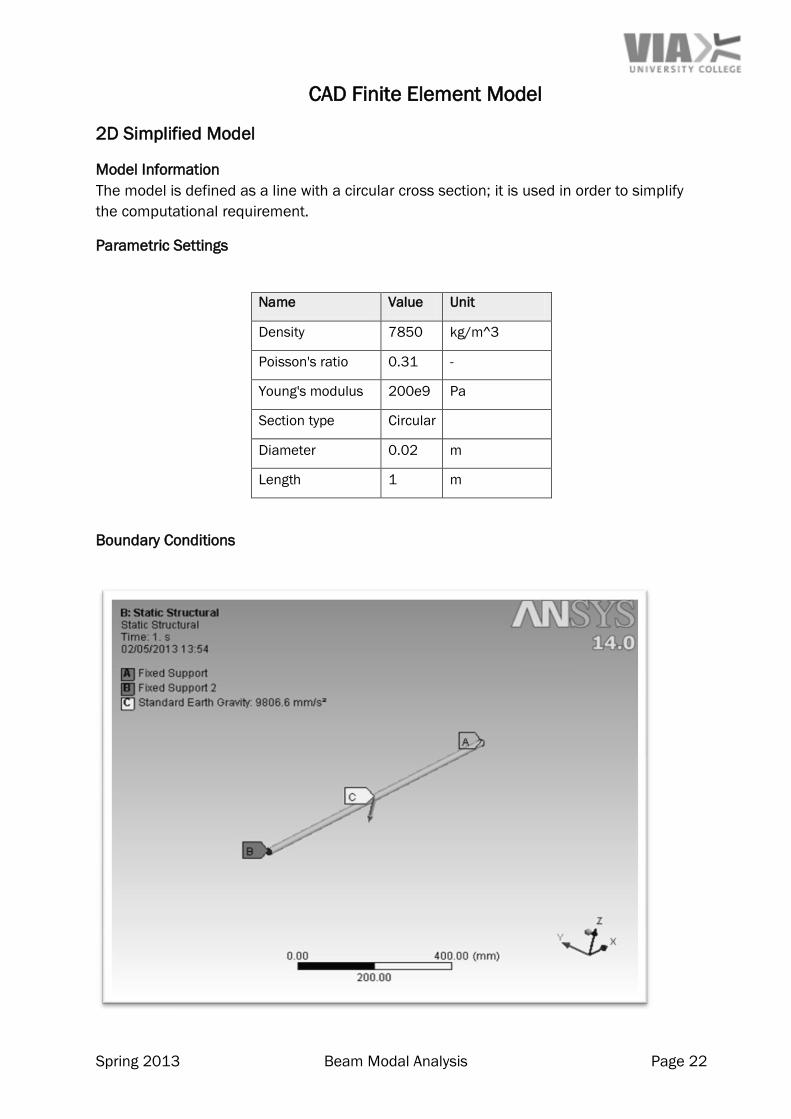
2D Simplified Model
Model Information
The model is defined as a line with a circular cross section; it is used in order to simplify
the computational requirement.
Parametric Settings
Name Value Unit
Density 7850 kg/m^3
Poisson's ratio 0.31 -
Young's modulus 200e9 Pa
Section type Circular
Diameter 0.02 m
Length 1 m
Boundary Conditions
Spring 2013 Beam Modal Analysis Page 23
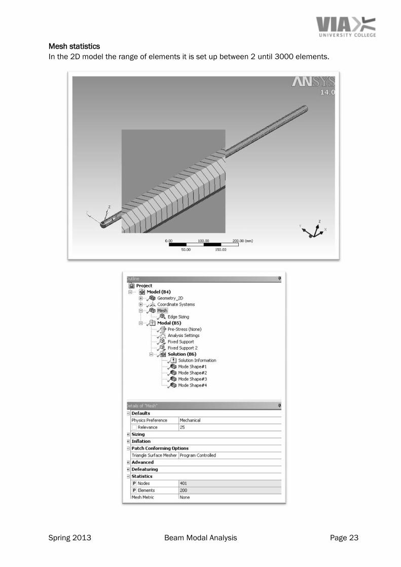
Mesh statistics
In the 2D model the range of elements it is set up between 2 until 3000 elements.
Spring 2013 Beam Modal Analysis Page 24
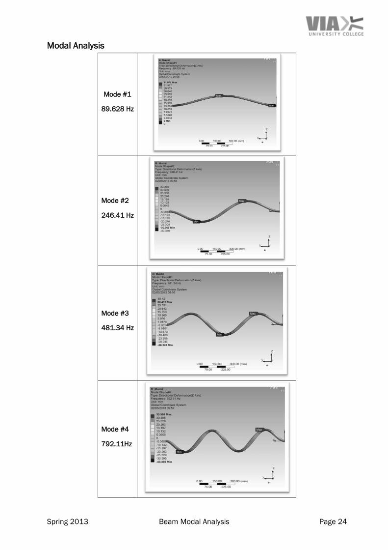
Modal Analysis
Mode #1
89.628 Hz
Mode #2
246.41 Hz
Mode #3
481.34 Hz
Mode #4
792.11Hz
Spring 2013 Beam Modal Analysis Page 25
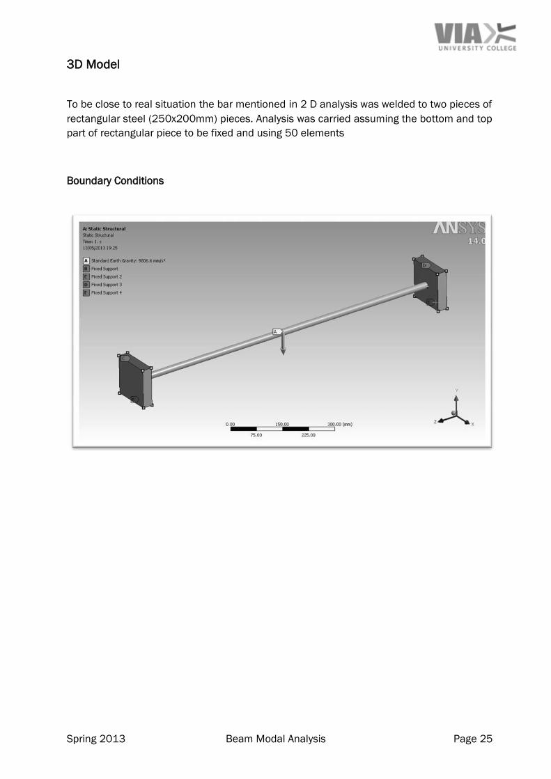
3D Model
To be close to real situation the bar mentioned in 2 D analysis was welded to two pieces of
rectangular steel (250x200mm) pieces. Analysis was carried assuming the bottom and top
part of rectangular piece to be fixed and using 50 elements
Boundary Conditions
Spring 2013 Beam Modal Analysis Page 26
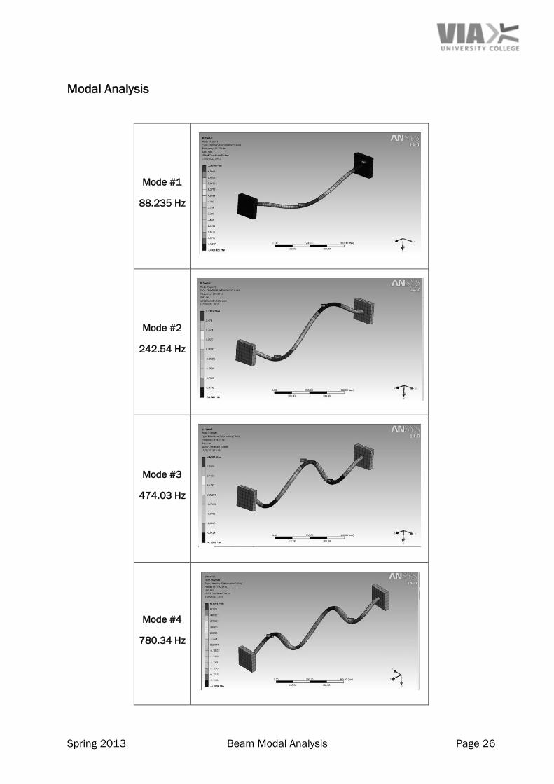
Modal Analysis
Mode #1
88.235 Hz
Mode #2
242.54 Hz
Mode #3
474.03 Hz
Mode #4
780.34 Hz
Spring 2013 Beam Modal Analysis Page 27
FEM Results Analysis
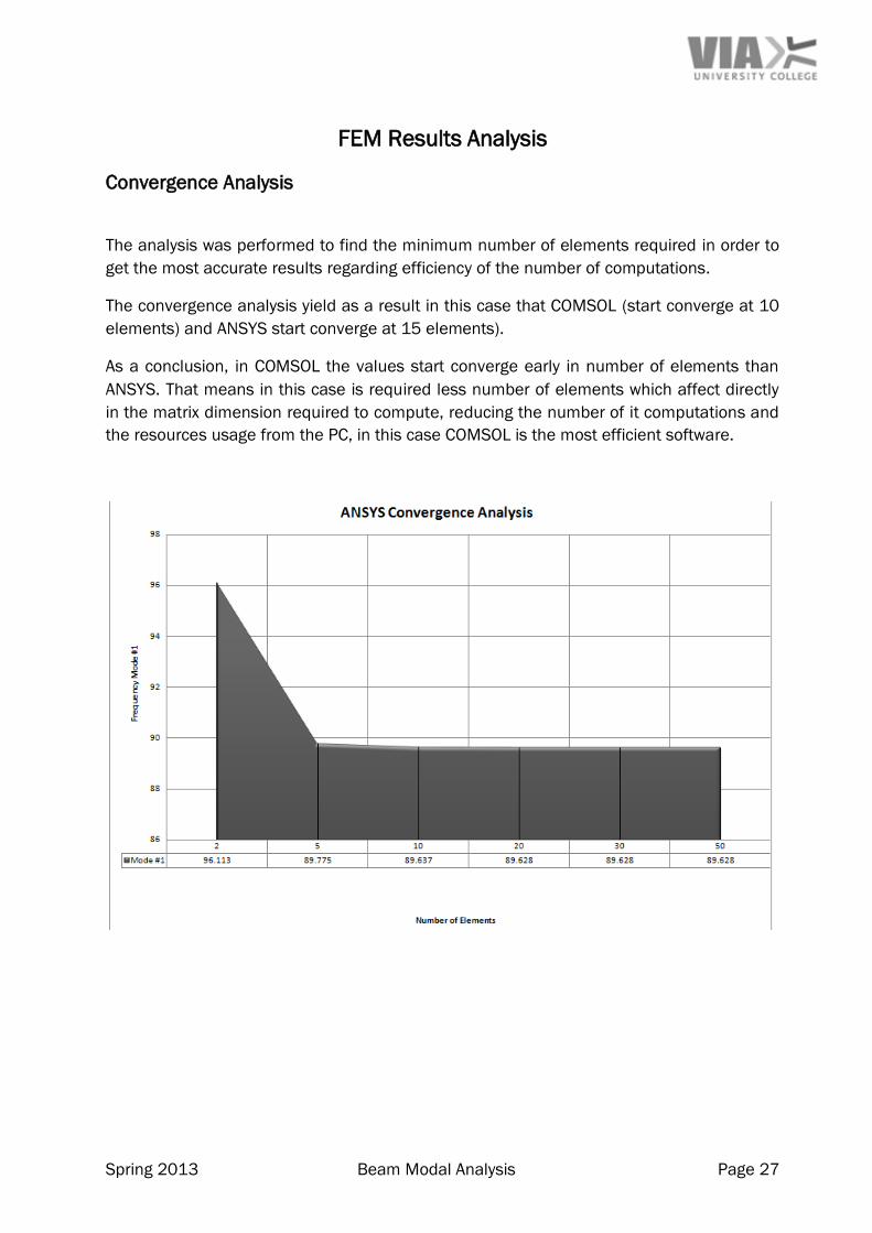
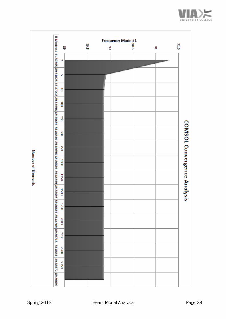
Convergence Analysis
The analysis was performed to find the minimum number of elements required in order to
get the most accurate results regarding efficiency of the number of computations.
The convergence analysis yield as a result in this case that COMSOL (start converge at 10
elements) and ANSYS start converge at 15 elements).
As a conclusion, in COMSOL the values start converge early in number of elements than
ANSYS. That means in this case is required less number of elements which affect directly
in the matrix dimension required to compute, reducing the number of it computations and
the resources usage from the PC, in this case COMSOL is the most efficient software.
Spring 2013 Beam Modal Analysis Page 28
Spring 2013 Beam Modal Analysis Page 29
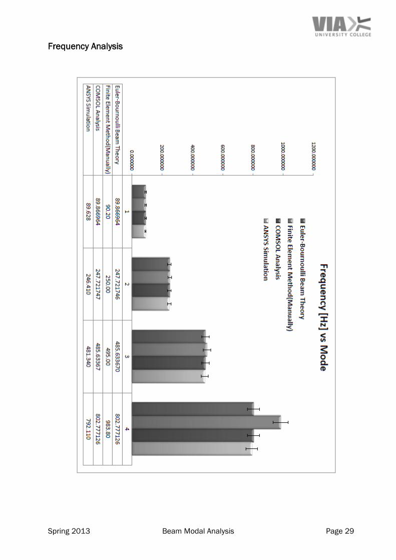
Frequency Analysis
Spring 2013 Beam Modal Analysis Page 30
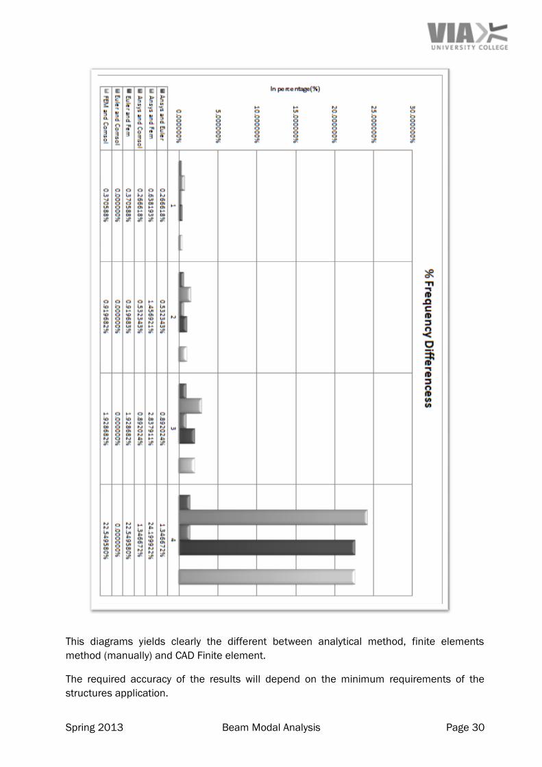
This diagrams yields clearly the different between analytical method, finite elements
method (manually) and CAD Finite element.
The required accuracy of the results will depend on the minimum requirements of the
structures application.
Spring 2013 Beam Modal Analysis Page 31
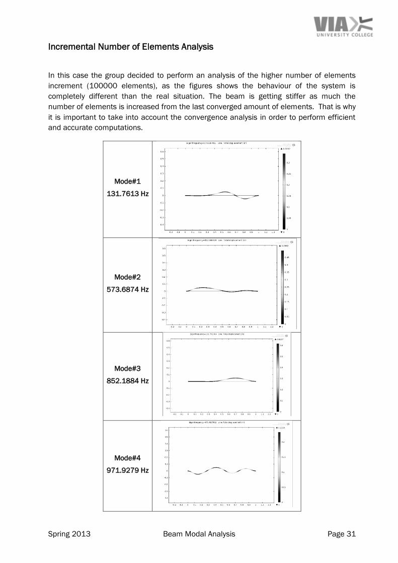
Incremental Number of Elements Analysis
In this case the group decided to perform an analysis of the higher number of elements
increment (100000 elements), as the figures shows the behaviour of the system is
completely different than the real situation. The beam is getting stiffer as much the
number of elements is increased from the last converged amount of elements. That is why
it is important to take into account the convergence analysis in order to perform efficient
and accurate computations.
Mode#1
131.7613 Hz
Mode#2
573.6874 Hz
Mode#3
852.1884 Hz
Mode#4
971.9279 Hz
Spring 2013 Beam Modal Analysis Page 32
Results Comparison of FEM to Beam Theory
In general, the displacement evaluated by FEM using the cubic function approximation for
δ(x), is lower than those of the beam theory except at the nodes. This is true for beams
subjected to some form of distributed load that are modelled using the cubic displacement
approximation function. The exception to this result is at the nodes, where the beam
theory and FEM results are identical because of the work – equivalent discrete loads at
the nodes.
The beam theory solution predicts a quartic (fourth – order) polynomial expression for
beam subjected to uniformly distributed loading, while the FEM solution δ(x) assumes a
cubic (third – order) displacement behaviour in each beam all load conditions(Under
uniformly distributed loading conditions, the beam theory solutions predicts a quadratic
moment and linear shear force in the beam. The FEM solution using the cubic
displacement function predicts a linear bending moment and a constant shear force within
each element used in the model.).
The FEM solution predicts a stiffer structure than the actual one. However, as more
elements are used in the model, the FEM solution converges to the beam theory solution.
The group has to mention that until this part of the entire project (which is basically a
simple structure) that the most relevant knowledge acquired is how powerful FEM can be
especially in the computation of complex structures or designs, but requires a real
understanding of the limitations of the method itself, or may cause serious errors.
Spring 2013 Beam Modal Analysis Page 33
Experimental Modal Analysis
Spring 2013 Beam Modal Analysis Page 34
Problem Definition
As it is already stated in the beginning of this project the main purpose of this experiment
it is to find at least the lower natural frequency of the fixed-fixed beam, which is the most
important considering structural design and the phenomenal behaviour of it when reach
that frequency(resonance).
The group has to emphasize in this point because regarding the complexity of a real
situation could be expected that to find a higher natural frequencies it is not be possible to
perform.
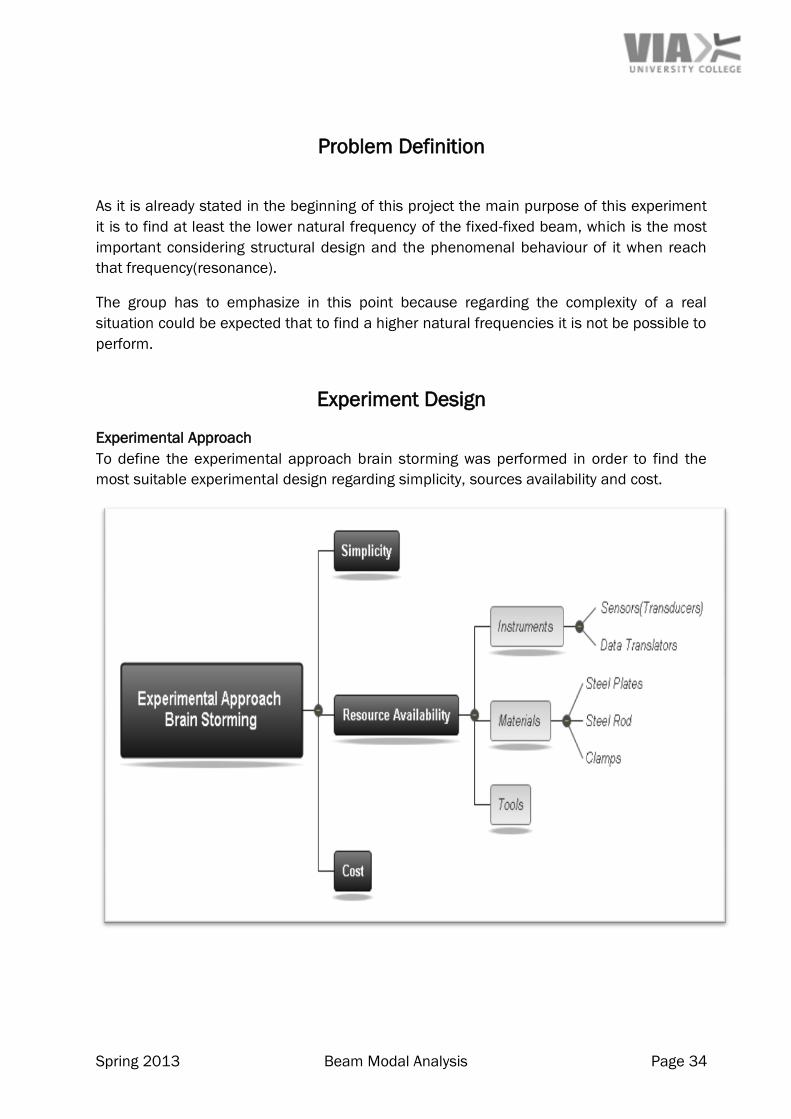
Experiment Design
Experimental Approach
To define the experimental approach brain storming was performed in order to find the
most suitable experimental design regarding simplicity, sources availability and cost.
Spring 2013 Beam Modal Analysis Page 35
Analytical Model
The analytical model is performed on the first part of this report and compared with the
CAD model. This model will be use full to analyse the data gather on the experiment.
Measured Variables
Considering the nature of the experiment and the purpose of it, the most relevant variable
which the experiment will evaluate is the natural frequency at different values of inputs.
It is expected that the natural frequency does not change over the different inputs; of
course the amplitude will change but in this case it not relevant.
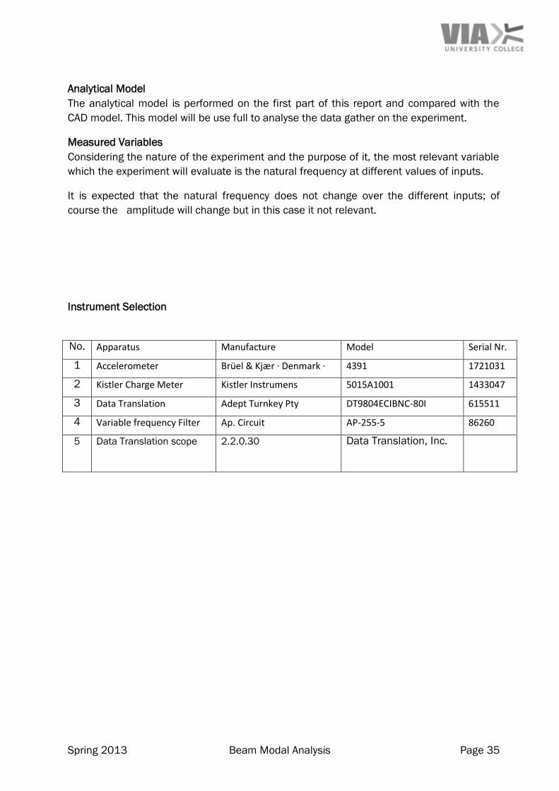
Instrument Selection
No. Apparatus Manufacture Model Serial Nr.
1 Accelerometer Brüel & Kjær · Denmark · 4391 1721031
2 Kistler Charge Meter Kistler Instrumens 5015A1001 1433047
3 Data Translation Adept Turnkey Pty DT9804ECIBNC-80I 615511
4 Variable frequency Filter Ap. Circuit AP-255-5 86260
5 Data Translation scope 2.2.0.30 Data Translation, Inc.
Spring 2013 Beam Modal Analysis Page 36
Spring 2013 Beam Modal Analysis Page 37
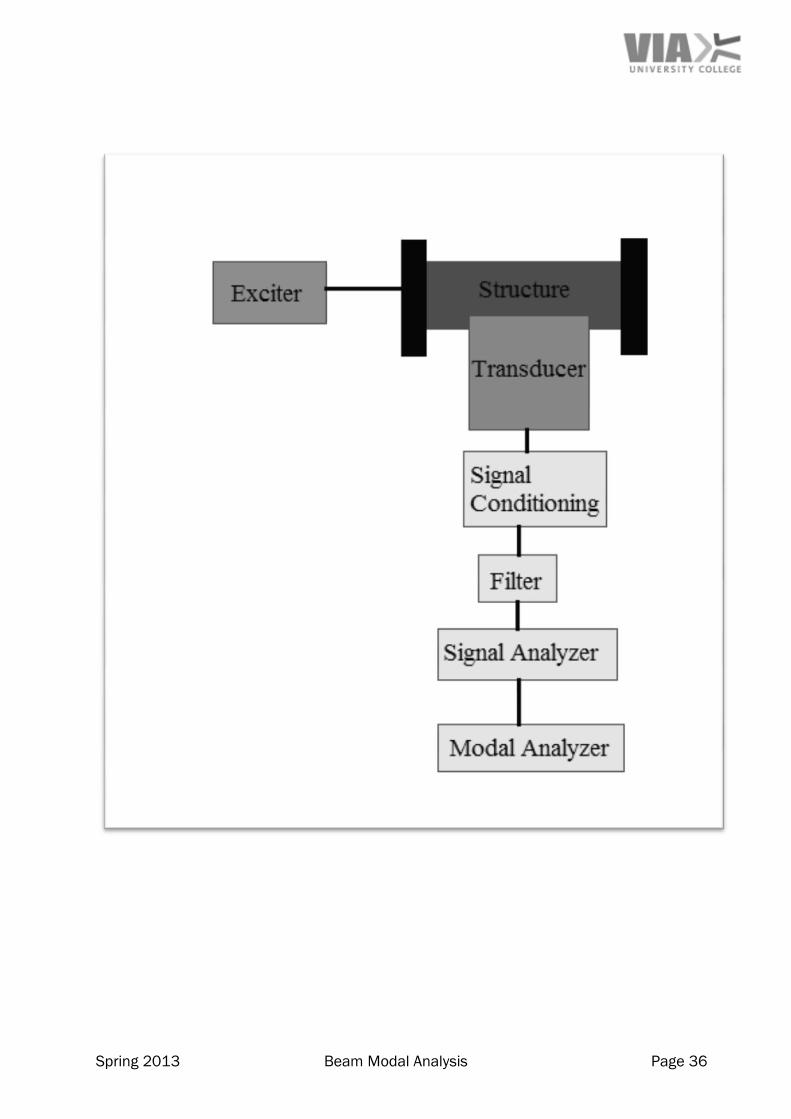
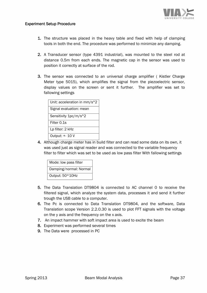
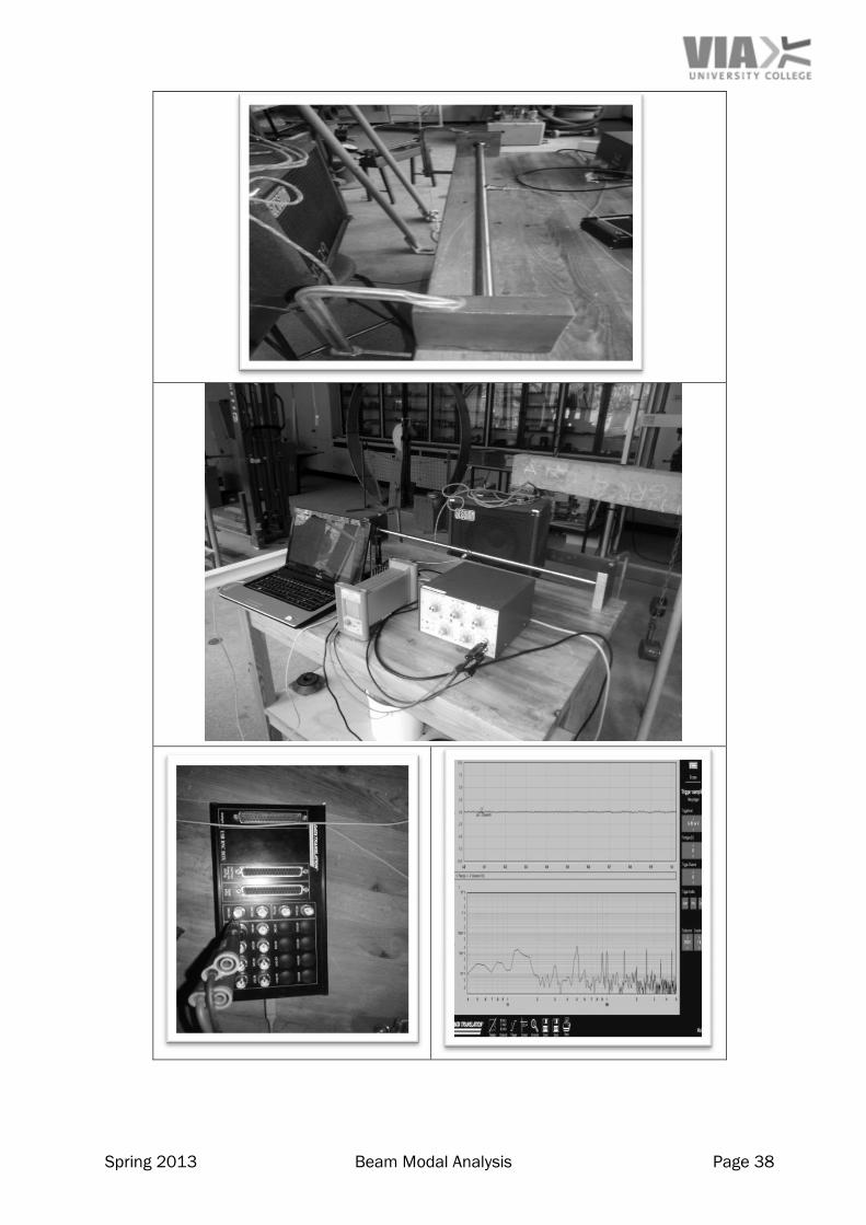
Experiment Setup Procedure
1. The structure was placed in the heavy table and fixed with help of clamping
tools in both the end. The procedure was performed to minimize any damping.
2. A Transducer sensor (type 4391 industrial), was mounted to the steel rod at
distance 0.5m from each ends. The magnetic cap in the sensor was used to
position it correctly at surface of the rod.
3. The sensor was connected to an universal charge amplifier ( Kistler Charge
Meter type 5015), which amplifies the signal from the piezoelectric sensor,
display values on the screen or sent it further. The amplifier was set to
fallowing settings
Unit: acceleration in mm/s^2
Signal evaluation: mean
Sensitivity 1pc/m/s^2
Filter 0.1s
Lp filter: 2 kHz
Output: +- 10 V
4. Although charge meter has in build filter and can read some data on its own, it
was used just as signal reader and was connected to the variable frequency
filter to filter which was set to be used as low pass filter With fallowing settings
Mode: low pass filter
Damping/normal: Normal
Output: 50*10Hz
5. The Data Translation DT9804 is connected to AC channel 0 to receive the
filtered signal, which analyze the system data, processes it and send it further
trough the USB cable to a computer.
6. The Pc is connected to Data Translation DT9804, and the software, Data
Translation scope Version 2.2.0.30 is used to plot FFT signals with the voltage
on the y axis and the frequency on the x axis.
7. An impact hammer with soft impact area is used to excite the beam
8. Experiment was performed several times
9. The Data were processed in PC
Spring 2013 Beam Modal Analysis Page 38
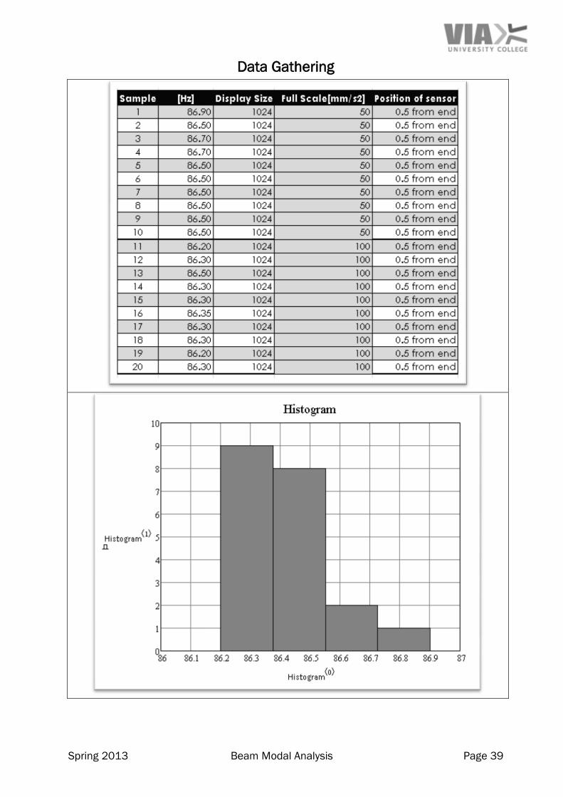
Spring 2013 Beam Modal Analysis Page 39
Data Gathering
Spring 2013 Beam Modal Analysis Page 40
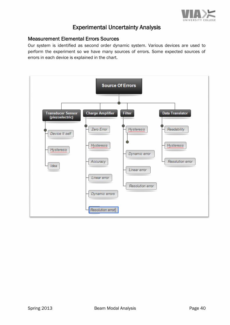
Experimental Uncertainty Analysis
Measurement Elemental Errors Sources
Our system is identified as second order dynamic system. Various devices are used to
perform the experiment so we have many sources of errors. Some expected sources of
errors in each device is explained in the chart.
Spring 2013 Beam Modal Analysis Page 41
Systematic Errors
Zero error
Calibration error or zero error is the systematic error caused by wrong Calibration of
measuring instruments. This kind of errors can be corrected to some extend my
calibrating instrument as precise as possible but some residual errors will still
persist. They are also caused because relation between input and output in the
instrument is not always linear. In special case of ours we have this kind of errors in
sensors and charge amplifier. Amplifier manufacturer has provided some data
about uncertainty caused by zero error but it is difficult to find data for sensor as
the error depends not only in instrument but also the way it will be used.
Insertion errors
This kind of error is cause because measurement device may not be correctly
placed. In our case flat magnetic transducer sensor may not be mounted tangential
to surface of the circular beam, whose natural frequency is to be measured.
Errors from surrounding
Experiment we are performing is likely to be influenced by surrounding noises.
Random errors
The errors which occur while taking repeated measurement with same parameters
are random errors. As our experiment is surrounded by multiple electric and
magnetic fields this kind of errors are certain. Amplifier may produce different data
in different measurement because of change of temperature in components over
time. Consideration will be taken properly to minimize this kind of errors.
Accuracy errors:
This error comes from accuracy of measurement by instrument. Instrument we are
using have certain percentage of accuracy for specific range. Instruments will be
used in the range where these errors can influence our result minimum.
Hysteresis:
In experiment same value of measurand, can be read differently depending if
reading was taken when values were increasing or decreasing. This phenomenon
occurs because of friction, mechanical flexure or electric capacitance. If reading
could be taken always at same point this error can be treated as systemic error but
since that cannot be done it can be classified as random error.
Resolution error:
As multiple instruments will be used, it is expected instruments will make reading in
discrete steps instead of continuous, resulting these kind of errors. Incorrectly
readability of outputs is also kind of resolution error.
Spring 2013 Beam Modal Analysis Page 42
Linearity errors
Output is expected to be proportional to input .If systematic errors at different point
is known calculated value must satisfy general relation between input and output.
But that may not be accurate or constant value. This deviation is linearity error.
Other errors
Thermal errors and sensibility errors can be both cause systematic and random
errors.
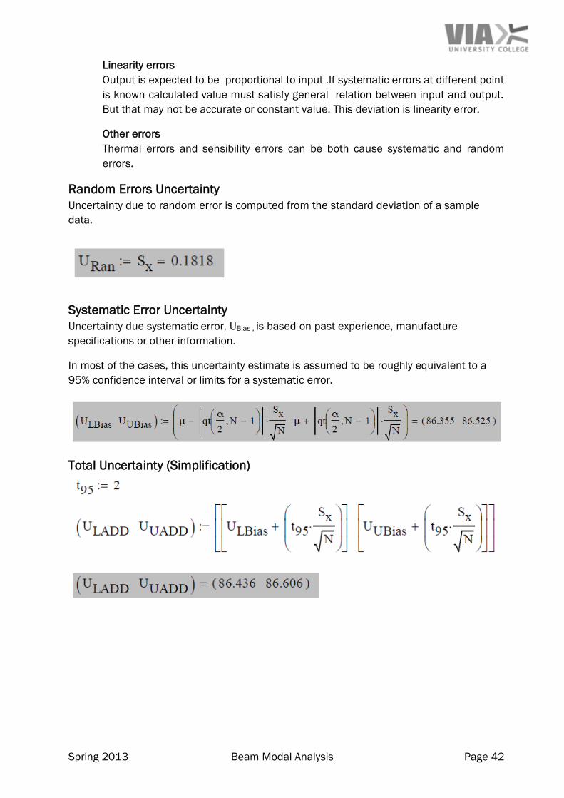
Random Errors Uncertainty
Uncertainty due to random error is computed from the standard deviation of a sample
data.
Systematic Error Uncertainty
Uncertainty due systematic error, UBias , is based on past experience, manufacture
specifications or other information.
In most of the cases, this uncertainty estimate is assumed to be roughly equivalent to a
95% confidence interval or limits for a systematic error.
Total Uncertainty (Simplification)
Spring 2013 Beam Modal Analysis Page 43
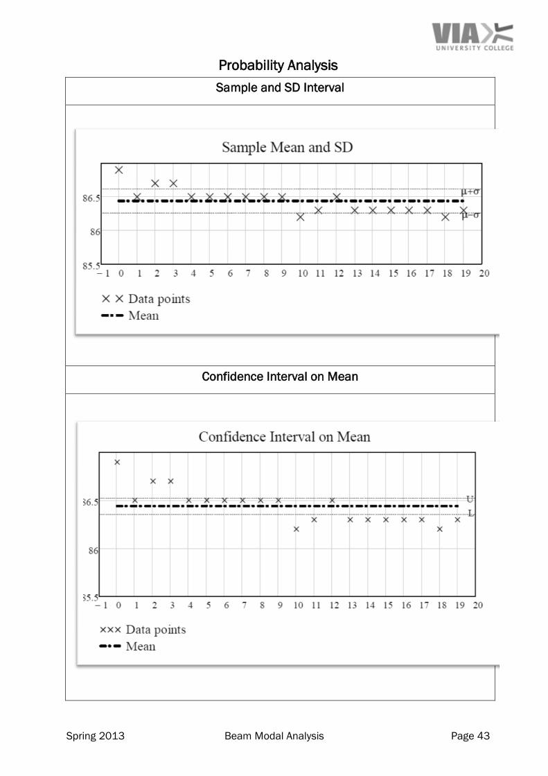
Probability Analysis
Sample and SD Interval
Confidence Interval on Mean
Spring 2013 Beam Modal Analysis Page 44
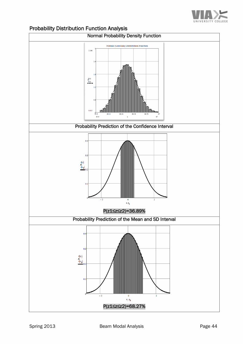
Probability Distribution Function Analysis
Normal Probability Density Function
Probability Prediction of the Confidence Interval
P(z1≤z≤z2)=36.89%
Probability Prediction of the Mean and SD Interval
P(z1≤z≤z2)=68.27%
Spring 2013 Beam Modal Analysis Page 45
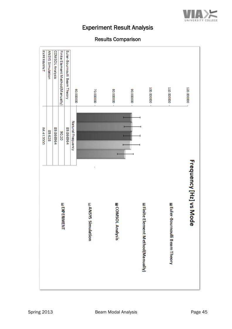
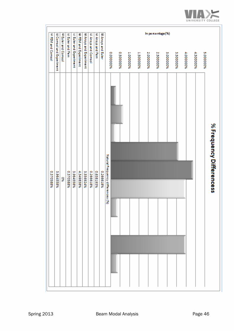
Experiment Result Analysis
Results Comparison
Spring 2013 Beam Modal Analysis Page 46

Spring 2013 Beam Modal Analysis Page 47
Conclusions
The charts shows that the experimental result differs less than 3.5 % from result obtained
from CAD software and 4 % with analytical results obtained from the beam theory. Thus
theory and results from experiment agree reasonably well.
The lower value of frequency obtained from experiment can be explained as the difference
in boundary condition of real situation. Analytical calculation and CAD simulation assumes
to have perfect clamped- clamped boundary, which defines system to be stiffer than the
real model. Real model was clamped, but possibility of slight movement existed.
The total uncertainty is located in the confidence interval (of 95%) between (86.436
86.606) with a 33.46 % of probability of occurrence in the experiment. The experiment
was repeated and replicated but of course there is place for many improvements.
It has to be mentioned that the project provided very good understanding of the theory,
use of computer software and the experimental procedures. It also gave insight to how
different approach can be used to find the same result.
Computer tools can be powerful in computation of complex structure but requires a real
understanding and limitation of method itself. Real life situation will always vary from
theory to certain extend and those consideration must be made. Use of Computer software
without understanding the real situation can be very dangerous and experimental test
should often verify the results unless the theory is understood clearly.
The subject of project was simple structure, none the less it required a lot of self-studying
in many fields and required deeper mathematical understanding. But under pressure is
when you stretch and put yourself in test. The group believes it was successful in that test.
Spring 2013 Beam Modal Analysis Page 48
List of Reference
1. Meriam, J. L., 2006, Engineering Mechanics: Static. 6th ed.
2. Boresi, A. P. and Schmidt R. J, 2009, Advanced mechanics of materials,, Wiley
3. Hibbeler, R. C., 2010, Engineering Mechanics Dynamics, 12th ed. Prentice Hall
4. Hibbeler, R. C., 2011, Mechanics of Materials, 8th ed. Prentice Hall
5. Engineering Vibrations Daniel J. Inman
6. Vibration Simulation using Matlab and ANSYS Michael R. Hatch
7. Advanced Modern Engineering Mathematics 4th Glyn James
8. Mathematical Methods for Mechanics Eckart W. Gekeler
9. Introduction to Engineering Experimentation Anthony J. Wheeler
10. Matlab
11. Mathcad
12. Inventor
13. ANSYS
14. COMSOL
15. E. and F.N spoon,1991,3rd edition, Noise control in industries
16. Inman, D J, 3rd edition, Engineering Vibration
17. Mathur, D.S 2005,Mechanics
18. Various Internet journal

Spring 2013 Beam Modal Analysis Page 49
Appendix
Appendix 1: Static Analysis
Appendix 2: Euler – Bernoulli Beam Modal Analysis
Appendix 3: Finite Element Method
FEM Calculations
Global Mass and Stiffness Matrix
Appendix 4: Probability Analysis
Appendix 5: Uncertainty Analysis