Beam Dynamics and FEL Simulations for FLASH

Igor Zagorodnov and Martin Dohlus08.02.2010

Beam Dynamics Meeting, DESY

FLASH Iparameters

ACC39

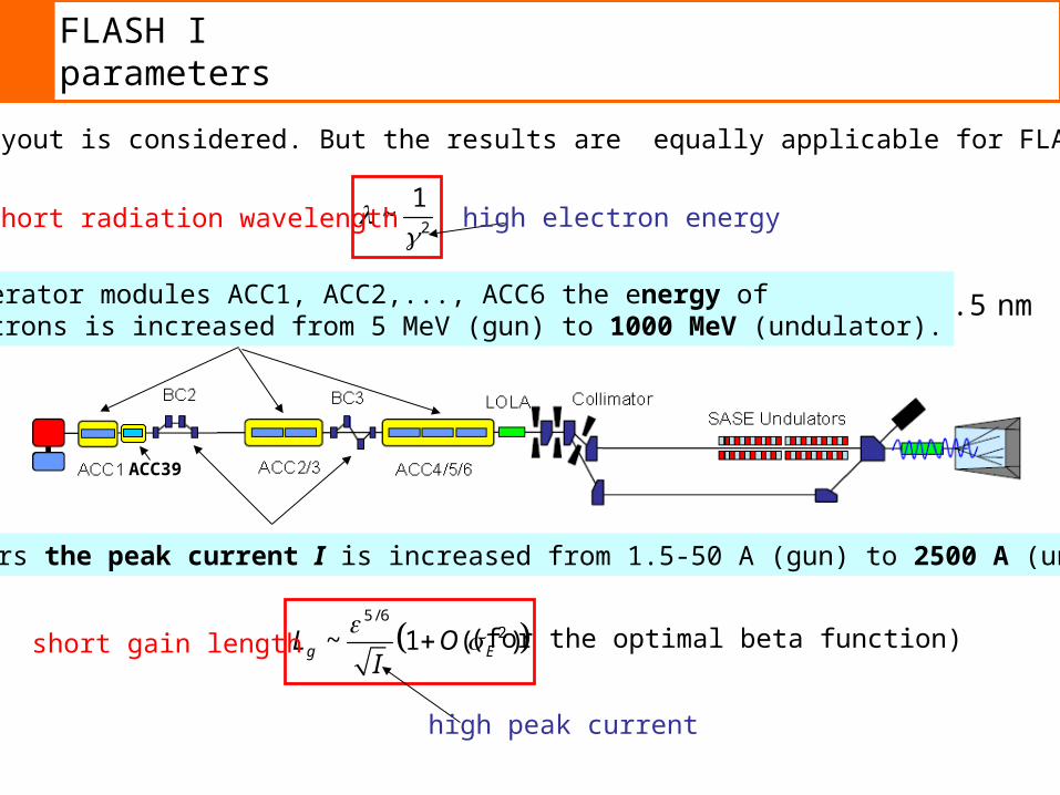
FLASH I layout is considered. But the results are equally applicable for FLASH II (SASE).

5 / 6

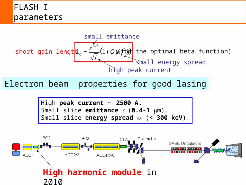
2~ 1 ( )g EL OI

short gain length (for the optimal beta function)

high peak current

2

1~

short radiation wavelength high electron energy

~ 6.5 nmIn accelerator modules ACC1, ACC2,..., ACC6 the energy of the electrons is increased from 5 MeV (gun) to 1000 MeV (undulator).

In compressors the peak current I is increased from 1.5-50 A (gun) to 2500 A (undulator).

FLASH Iparameters

Electron beam properties for good lasing

High peak current ~ 2500 A. Small slice emittance (0.4-1 m).Small slice energy spread E(< 300 keV).

5 / 6

2~ 1 ( )g EL OI

short gain length (for the optimal beta function)

small energy spread

small emittance

high peak current

High harmonic module in 2010

FLASH Iparameters

ACC39

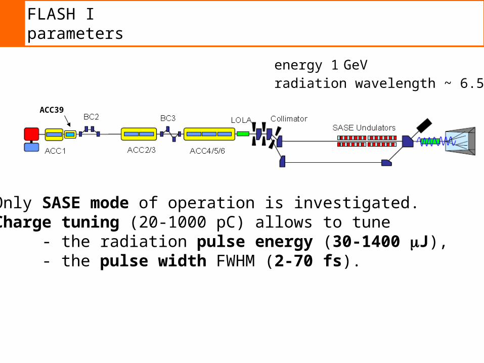
energy 1 GeVradiation wavelength ~ 6.5 nm

Only SASE mode of operation is investigated.Charge tuning (20-1000 pC) allows to tune

- the radiation pulse energy (30-1400 J), - the pulse width FWHM (2-70 fs).

FLASH Iparameters

ACC39

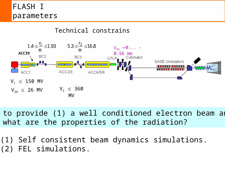
r56 0... -0.56 mm

Technical constrains

V1 150 MV

V39 26 MV V2 360 MV

11.4 1.93m

r 25.3 16.8

m

r

How to provide (1) a well conditioned electron beam and (2) what are the properties of the radiation?

(1) Self consistent beam dynamics simulations.(2) FEL simulations.

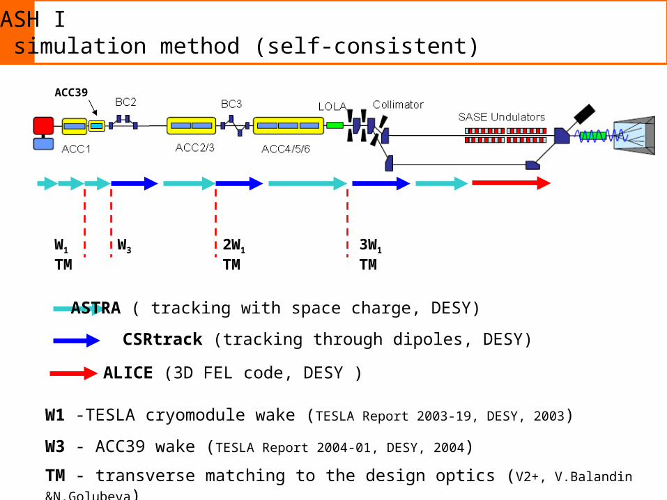
FLASH I3d simulation method (self-consistent)

ACC39

W3 2W1

TM3W1

TMW1

TM

ASTRA ( tracking with space charge, DESY)

CSRtrack (tracking through dipoles, DESY)

W1 -TESLA cryomodule wake (TESLA Report 2003-19, DESY, 2003)

W3 - ACC39 wake (TESLA Report 2004-01, DESY, 2004)

TM - transverse matching to the design optics (V2+, V.Balandin &N.Golubeva)

ALICE (3D FEL code, DESY )

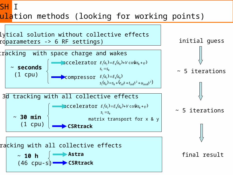
FLASH Isimulation methods (looking for working points)

1d tracking with space charge and wakes

compressor

3d tracking with all collective effects

Astra

CSRtrack

quasi 3d tracking with all collective effects

accelerator 01

00011 cos

ss

ksVsEsE

3

56662

56656001

0011

utrsss

sEsE

accelerator 01

00011 cos

ss

ksVsEsE

matrix transport for x & y

CSRtrack

~ 10 h (46 cpu-s)

~ seconds(1 cpu)

~ 30 min (1 cpu)

1d analytical solution without collective effects(8 macroparameters -> 6 RF settings) initial guess

~ 5 iterations

~ 5 iterations

final result

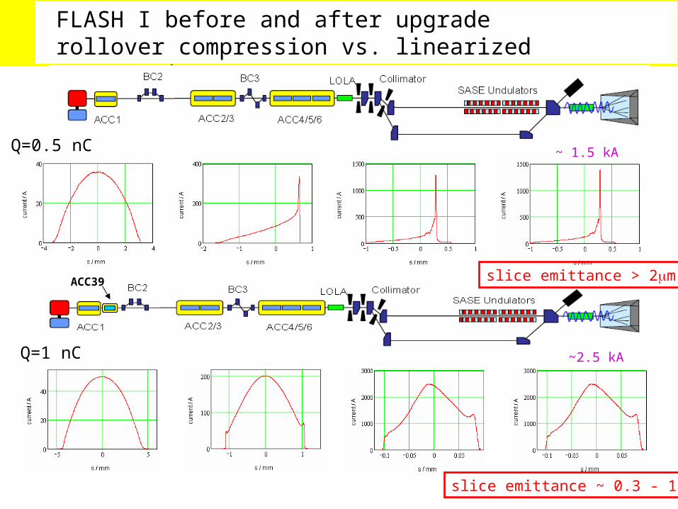
FLASH I before and after upgrade rollover compression vs. linearized compression

~ 1.5 kA

ACC39

~2.5 kA

slice emittance > 2m

slice emittance ~ 0.3 - 1m

Q=1 nC

Q=0.5 nC

20 40 60 80 100 1200

10

20

30

40

50

20 40 60 80 100 1200

5

10

15

20

25

30

35

[m]z

[ ]x m

[m]z

[ ]y m

new

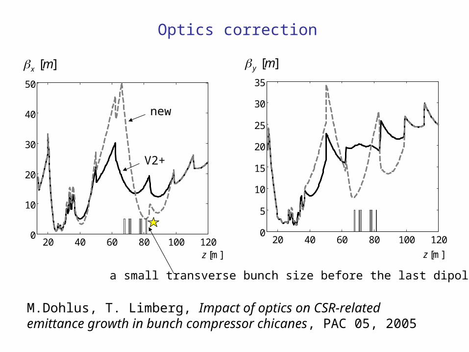
Optics correction

M.Dohlus, T. Limberg, Impact of optics on CSR-related emittance growth in bunch compressor chicanes, PAC 05, 2005

V2+

a small transverse bunch size before the last dipole

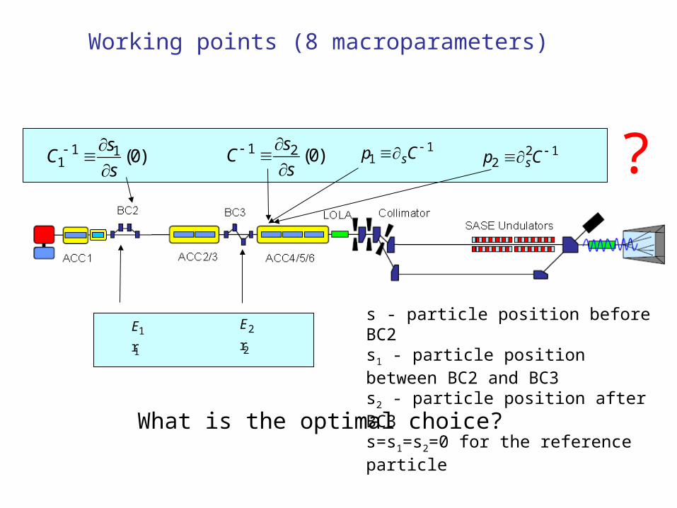
Working points (8 macroparameters)

1

1r

E 2

2r

E

11 sp C 1 1

1 (0)s

Cs

1 2 (0)

sC

s

?2 1

2 sp C

What is the optimal choice?

s - particle position before BC2s1 - particle position between BC2 and BC3s2 - particle position after BC3s=s1=s2=0 for the reference particle

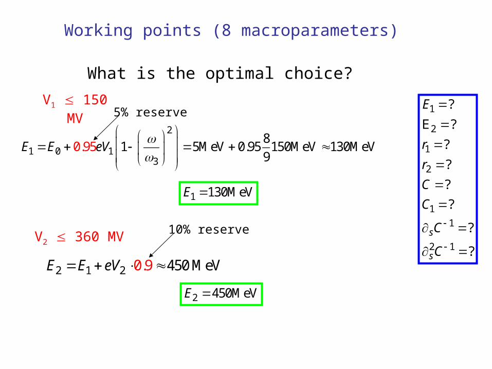
Working points (8 macroparameters)

What is the optimal choice?

V1 150 MV

V2 360 MV

2

1 0 13

81 5MeV 0.95 150MeV 130 95 Me. 0 V

9E E eV

1 130MeVE

2 1 2 0.9 450 MeVE E eV

5% reserve

10% reserve

2 450MeVE

1

2

1

2

1

1

2 1

?

E ?

?

?

?

?

?

?

s

s

E

r

r

C

C

C

C

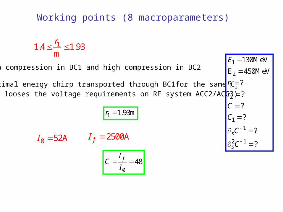
Working points (8 macroparameters)

11.4 1.93m

r

1 1.93mr

- low compression in BC1 and high compression in BC2

- maximal energy chirp transported through BC1for the same C1

(it looses the voltage requirements on RF system ACC2/ACC3)

0 52AI 2500AfI

0

48fIC

I

1

2

1

2

1

1

2 1

130MeV

E 450MeV

?

?

?

?

?

?

s

s

E

r

r

C

C

C

C

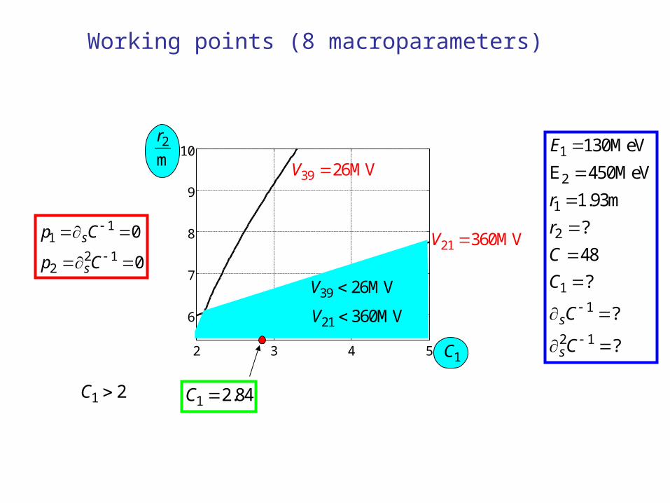
Working points (8 macroparameters)

2 3 4 5

6

7

8

9

10

1C

2

m

r

39 26MVV

21 360MVV

21 360MVV 39 26MVV

11

2 12

0

0

s

s

p C

p C

1 2.84C 1 2C

1

2

1

2

1

1

2 1

130MeV

E 450MeV

1.93m

?

48

?

?

?

s

s

E

r

r

C

C

C

C

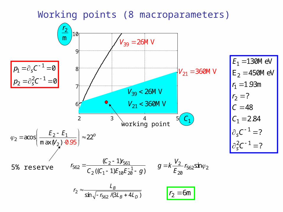
Working points (8 macroparameters)

2 3 4 5

6

7

8

9

10

1C

2

m

r

39 26MVV

21 360MVV

21 360MVV

working point

39 26MVV

11

2 12

0

0

s

s

p C

p C

2 12

2

acos 22ma 0.9x( 5)

oE E

V

5% reserve2 561

562 12 1 10 20

( 1)

(( 1) )

C rr

C C E E g

2562 2

20

sinV

g k rE

2562sin /(3 4 )

B

B D

Lr

r L L

2 6mr

1

2

1

2

1

1

2 1

130MeV

E 450MeV

1.93m

?

48

2.84

?

?

s

s

E

r

r

C

C

C

C

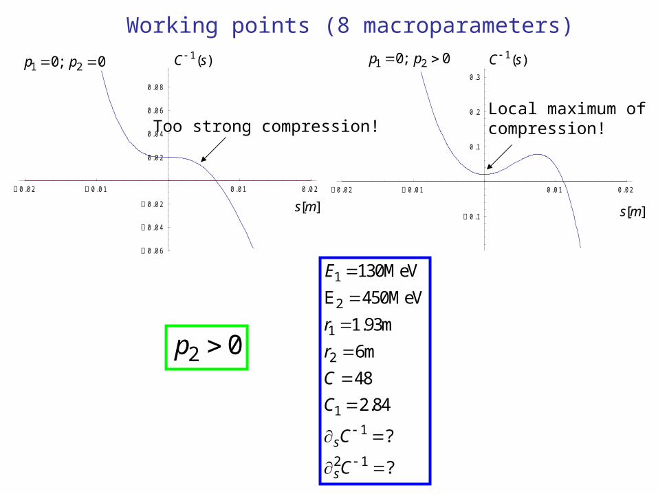
Working points (8 macroparameters)

0 .0 2 0 .0 1 0 .0 1 0 .0 2

0 .0 6

0 .0 4

0 .0 2

0 .0 2

0 .0 4

0 .0 6

0 .0 8

0 .0 2 0 .0 1 0 .0 1 0 .0 2

0 .1

0 .1

0 .2

0 .3

1( )C s

[ ]s m [ ]s m

1 20; 0p p

Too strong compression!Local maximum ofcompression!

1 20; 0p p 1( )C s

2 0p

1

2

1

2

1

1

2 1

130MeV

E 450MeV

1.93m

6m

48

2.84

?

?

s

s

E

r

r

C

C

C

C

0 2000 4000 6000 8000 100000.04

0.06

0.08

0.1

0.12

0.14

0.16

0 5000 10000 15000 200000

0.002

0.004

0.006

0.008

0.01

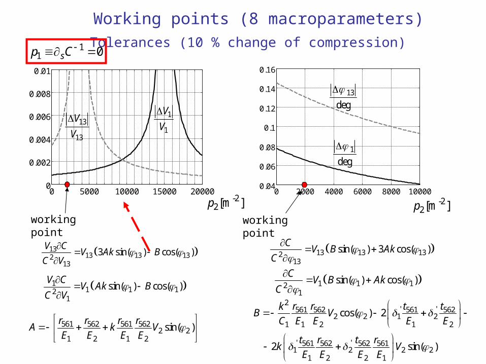
Working points (8 macroparameters)

Tolerances (10 % change of compression)

1

1

V

V

13

13

V

V

working point working point

1

deg

13

deg

11 1 12

1

sin( ) cos( )V C

V Ak BC V

1 1 12

1

sin( ) cos( )C

V B AkC

1313 13 132

13

3 sin( ) cos( )V C

V Ak BC V

13 13 132

13

sin( ) 3 cos( )C

V B AkC

11 0sp C

-22[m ]p -2

2[m ]p

561 562 561 5622 2

1 2 1 2

sin( )r r r r

A k VE E E E

2' '561 562 561 562

2 2 1 21 1 2 1 2

' '561 562 562 5611 2 2 2

1 2 2 1

cos( ) 2

2 sin( )

r r t tkB V

C E E E E

t r t rk V

E E E E

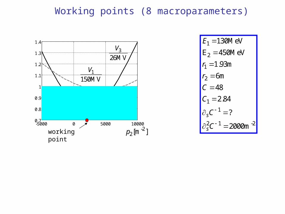
Working points (8 macroparameters)

-5000 0 5000 100000.7

0.8

0.9

1

1.1

1.2

1.3

1.4

1

150MV

V

3

26MV

V

-22[m ]pworking point

1

2

1

2

1

1

2 1 -2

130MeV

E 450MeV

1.93m

6m

48

2.84

?

2000m

s

s

E

r

r

C

C

C

C

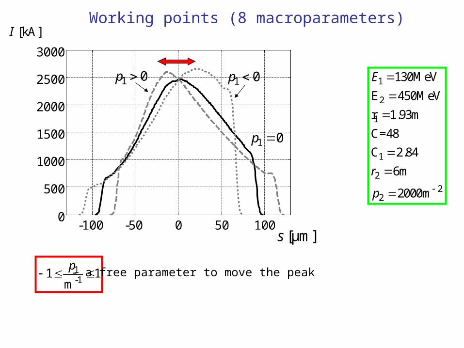
Working points (8 macroparameters)

1

2

1

1

2

22

130MeV

E 450MeV

r 1.93m

C=48

C 2.84

6m

2000m

E

r

p

1-1

1 1m

p

-100 -50 0 50 1000

500

1000

1500

2000

2500

3000

1 0p 1 0p

1 0p

[kA]I

[μm]s

- a free parameter to move the peak

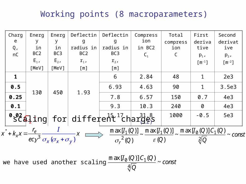
Charge

Q,

nC

Energy

in BC2

E1,

[MeV]

Energy

in BC3

E2,

[MeV]

Deflecting

radius in BC2

r1,

[m]

Deflecting

radius in BC3

r2,

[m]

Compression

in BC2

C1

Total

compression

C

First

derivative

p1,

[m-1]

Second

derivative

p2,

[m-2]

1

130 450 1.93

6 2.84 48 1 2e3

0.5 6.93 4.63 90 1 3.5e3

0.25 7.8 6.57 150 0.7 4e3

0.1 9.3 10.3 240 0 4e3

0.02 15.17 31.8 (12) 1000 -0.5 5e3

0 14

max[ ( )] ( )~

I Q C Qconst

Q

1 :C

Working points (8 macroparameters)

scaling for different charges''

3 ( )e

yx

x x

rx k x

Ix

ec 0 11 1

2 2

max[ ( )] ( )max[ ( )] max[ ( )]~ ~ ~

( )( )r

I Q C QI Q I Qconst

Q QQ

we have used another scaling

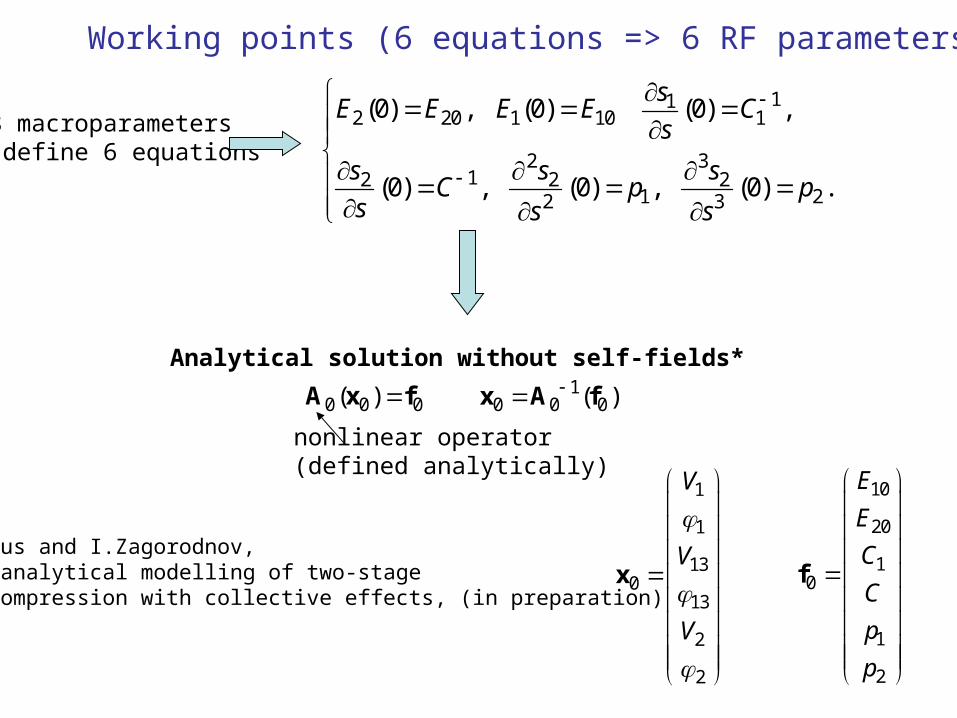
Working points (6 equations => 6 RF parameters)

112 20 1 10 1

2 312 2 2

1 22 3

(0) , (0) (0) ,

(0) , (0) , (0) .

sE E E E C

s

s s sC p p

s s s

Analytical solution without self-fields*

8 macroparameters define 6 equations

10 0 0( )x A f

1

1

130

13

2

2

V

V

V

x

10

20

10

1

2

E

E

C

C

p

p

f

0 0 0( ) A x f

nonlinear operator (defined analytically)

*M.Dohlus and I.Zagorodnov,A semi analytical modelling of two-stage bunch compression with collective effects, (in preparation)

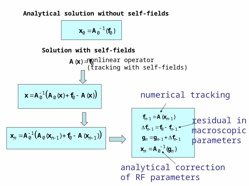
Analytical solution without self-fields

10 0 0( )x A f

Solution with self-fields

0( ) A x f

10 ( )n nx A g

nonlinear operator (tracking with self-fields)

1 1n n n g g f

10 0 0( ) ( ) x A A x f A x

10 0 1 0 1( ) ( )n n n

x A A x f A x

numerical tracking

analytical correction of RF parameters

1 1( )n n f A x

1 0 1n n f f fresidual inmacroscopic parameters

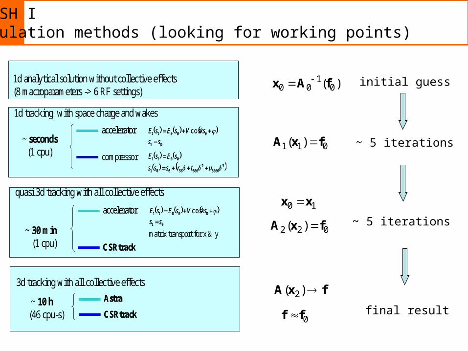
FLASH Isimulation methods (looking for working points)

initial guess

~ 5 iterations

~ 5 iterations

final result

1d tracking with space charge and wakes

compressor

3d tracking with all collective effects

Astra

CSRtrack

quasi 3d tracking with all collective effects

accelerator 01

00011 cos

ss

ksVsEsE

3

56662

56656001

0011

utrsss

sEsE

accelerator 01

00011 cos

ss

ksVsEsE

matrix transport for x & y

CSRtrack

~ 10 h(46 cpu-s)

~ seconds(1 cpu)

~ 30 min(1 cpu)

1d analytical solution without collective effects(8 macroparameters -> 6 RF settings)

1d tracking with space charge and wakes

compressor

3d tracking with all collective effects

AstraAstra

CSRtrackCSRtrack

quasi 3d tracking with all collective effects

accelerator 01

00011 cos

ss

ksVsEsE

accelerator

01

00011 cos

ss

ksVsEsE

3

56662

56656001

0011

utrsss

sEsE

3

56662

56656001

0011

utrsss

sEsE

accelerator 01

00011 cos

ss

ksVsEsE

accelerator

01

00011 cos

ss

ksVsEsE

matrix transport for x & y

CSRtrackCSRtrack

~ 10 h(46 cpu-s)

~ seconds(1 cpu)

~ 30 min(1 cpu)

1d analytical solution without collective effects(8 macroparameters -> 6 RF settings)

10 0 0( )x A f

1 1 0( ) A x f

2 2 0( ) A x f

2( ) A x f

0f f

0 1x x

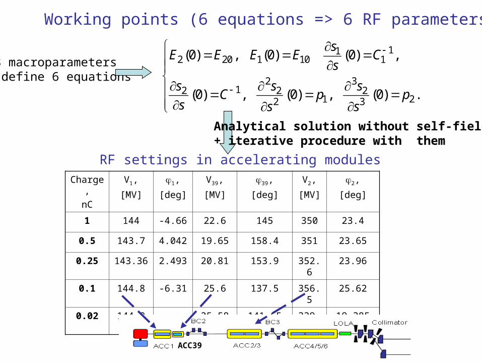
Working points (6 equations => 6 RF parameters)

112 20 1 10 1

2 312 2 2

1 22 3

(0) , (0) (0) ,

(0) , (0) , (0) .

sE E E E C

s

s s sC p p

s s s

Charge,

nC

V1,

[MV]

1,

[deg]

V39,

[MV]

39,

[deg]

V2,

[MV]

2,

[deg]

1 144 -4.66 22.6 145 350 23.4

0.5 143.7 4.042 19.65 158.4 351 23.65

0.25 143.36 2.493 20.81 153.9 352.6 23.96

0.1 144.8 -6.31 25.6 137.5 356.5 25.62

0.02 144.9 -3.894 25.58 141.65 339.8 19.385

RF settings in accelerating modules

Analytical solution without self-fields + iterative procedure with them

ACC39

8 macroparameters define 6 equations

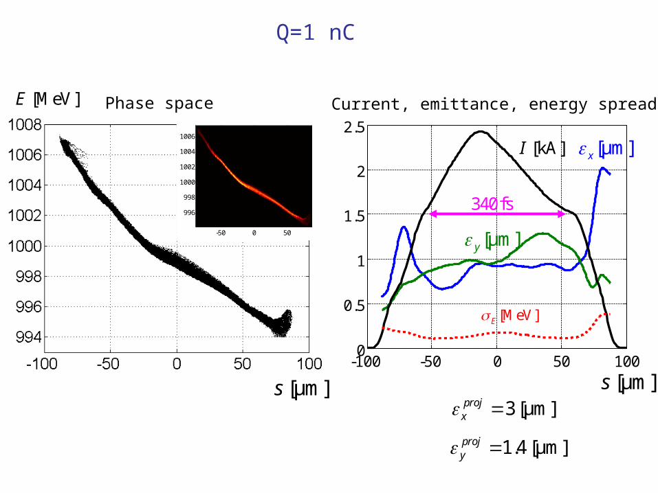
-100 -50 0 50 1000

0.5

1

1.5

2

2.5

Q=1 nC

[MeV]E

[kA]I

Phase space

[MeV]E

3 [μm]projx

1.4 [μm]projy

-50 0 50

996

998

1000

1002

1004

1006

Current, emittance, energy spread

[μm]x

[μm]y

[μm]s [μm]s

340fs

-60 -40 -20 0 20 40 600

0.5

1

1.5

2

2.5

Q=0.5 nC

[μm]s

[MeV]E

[kA]I

Phase space

[MeV]E

2.5 [μm]projx

0.84 [μm]projy

Current, emittance, energy spread

[μm]x

[μm]y

[μm]s

-50 0 50

998

1000

1002

1004

130fs

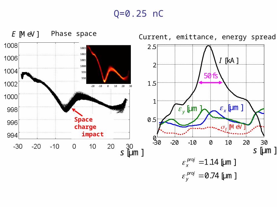
-30 -20 -10 0 10 20 300

0.5

1

1.5

2

2.5

Q=0.25 nC

[MeV]E

[kA]I

[μm]x

Phase space

[MeV]E

1.14 [μm]projx

0.74 [μm]projy

Current, emittance, energy spread

-20 -10 0 10 20 30

998

999

1000

1001

1002

1003

[μm]y

[μm]s [μm]s

Space charge impact

50fs

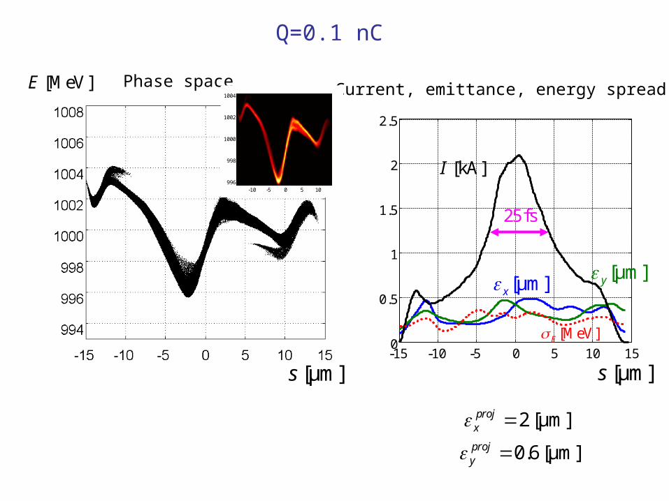
-15 -10 -5 0 5 10 150

0.5

1

1.5

2

2.5

Q=0.1 nC

[MeV]E

[kA]I

[μm]x

[MeV]E

Current, emittance, energy spread

2 [μm]projx

0.6 [μm]projy

[μm]y

Phase space

[μm]s [μm]s

-10 -5 0 5 10996

998

1000

1002

1004

25fs

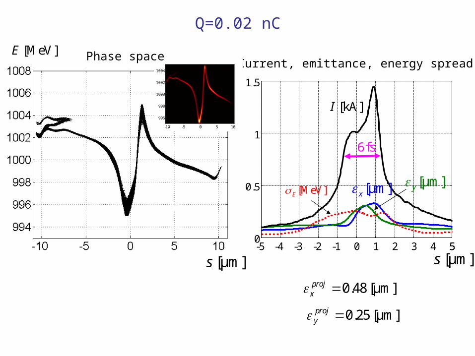
-5 -4 -3 -2 -1 0 1 2 3 4 550

0.5

1

1.5

Q=0.02 nC

[μm]s

[MeV]E

[kA]I

[μm]x[MeV]E

Current, emittance, energy spread

0.48 [μm]projx

0.25 [μm]projy

-10 -5 0 5 10

996

998

1000

1002

1004

[μm]y

[μm]s

Phase space

6fs

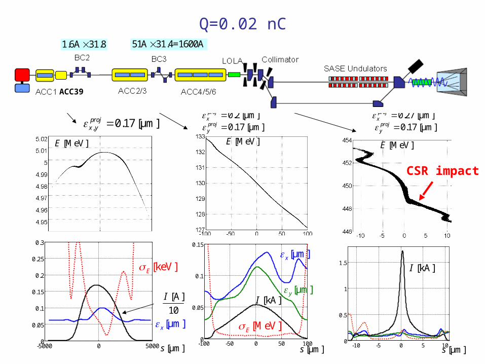
-100 -50 0 50 1000

0.05

0.1

0.15

Q=0.02 nC

-5000 0 50000

0.05

0.1

0.15

0.2

0.25

0.3

, 0.17 [μm]projx y

[A]

10

I

[μm]x

[keV]E

0.2 [μm]projx

0.17 [μm]projy

0.27 [μm]projx

0.17 [μm]projy

[kA]I

[μm]x

[MeV]E

[μm]y

-10 -5 0 5 100

0.5

1

1.5[kA]I

[μm]s

[MeV]E

[μm]s [μm]s

[MeV]E [MeV]E

ACC39

1.6A 31.8 51A 31.4=1600A

CSR impact

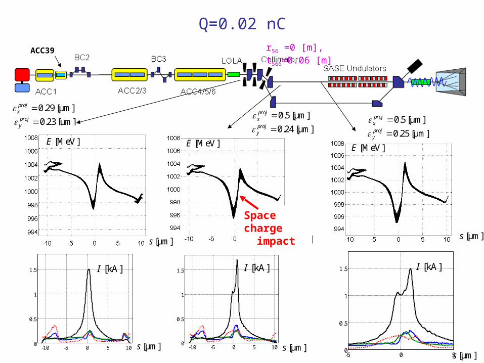
Q=0.02 nC

ACC39

0.5 [μm]projx

0.25 [μm]projy

-10 -5 0 5 100

0.5

1

1.5

0.29 [μm]projx

0.23 [μm]projy

-10 -5 0 5 100

0.5

1

1.5

0.5 [μm]projx

0.24 [μm]projy

r56 =0 [m], t566=0.06 [m]

-5 0 50

0.5

1

1.5 [kA]I[kA]I[kA]I

[μm]s [μm]s[μm]s

[μm]s [μm]s [μm]s

[MeV]E [MeV]E [MeV]E

Space charge impact

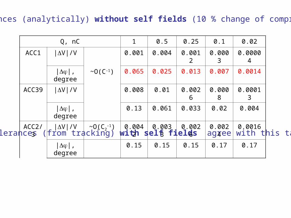
Tolerances (analytically) without self fields (10 % change of compression)

Tolerances (from tracking) with self fields agree with this table

Q, nC 1 0.5 0.25 0.1 0.02

ACC1 |V|/V

~O(C-1)

0.001 0.004 0.0012 0.0003 0.00004

||, degree 0.065 0.025 0.013 0.007 0.0014

ACC39 |V|/V 0.008 0.01 0.0026 0.0008 0.00013

||, degree 0.13 0.061 0.033 0.02 0.004

ACC2/3 |V|/V ~O(C2-1) 0.0042 0.0033 0.0026 0.0024 0.0016

||, degree 0.15 0.15 0.15 0.17 0.17

FLASHparameters

How to provide (1) a well conditioned electron beam and (2) what are the properties of the radiation?

(1) Self consistent beam dynamics simulations.We are able to provide the well conditioned electron beam for different charges. But RF tolerances for small charges are tough.

(2) FEL simulations (next slides).

-50 0 500

0.5

1

1.5

2

2.5

-2 -1 0 1 20

0.5

1

1.5

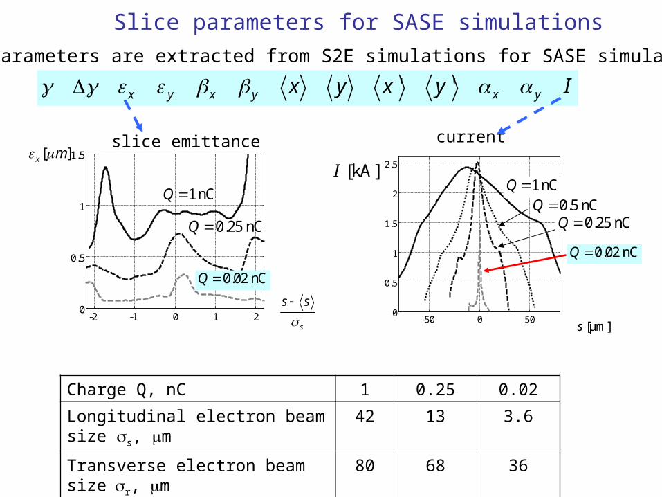
Charge Q, nC 1 0.25 0.02

Longitudinal electron beam size s, m

42 13 3.6

Transverse electron beam sizer, m 80 68 36

[μm]s

[ ]x m

Slice parameters for SASE simulations

s

s s

slice emittance

' 'x y x y x yx y x y I Slice parameters are extracted from S2E simulations for SASE simulations

current

1 nCQ

0.25 nCQ

0.02 nCQ

1 nCQ

0.02 nCQ

[kA]I

0.5 nCQ 0.25 nCQ

0 5 10 15 20 250

10

20

30

40

50

60

70

80

90

0 5 10 15 2010

-2

100

102

103

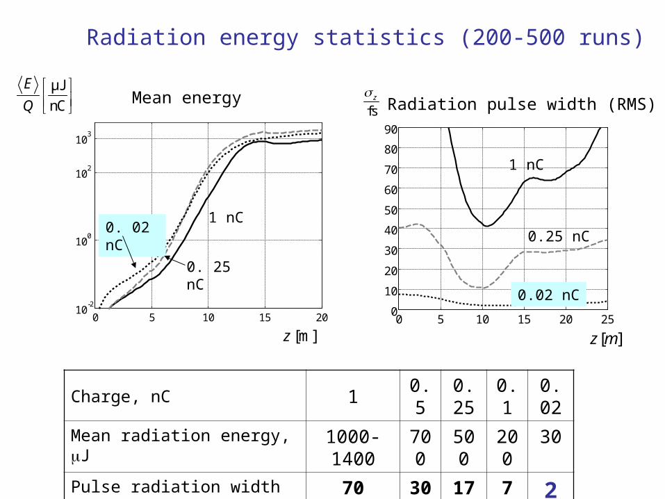
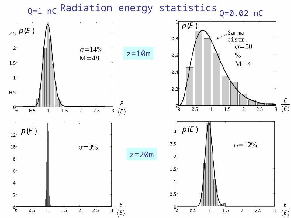
Radiation energy statistics (200-500 runs)

μJ

nC

E

Q

[m]z

0. 25 nC

1 nC

Mean energy

0. 02 nC

fsz

[ ]z m

1 nC

0.25 nC

0.02 nC

Radiation pulse width (RMS)

Charge, nC 1 0.5 0.25 0.1 0.02

Mean radiation energy, J 1000-1400

700 500 200 30

Pulse radiation width (FWHM), fs

70 30 17 7 2

0 0.5 1 1.5 2 2.5 30

0.2

0.4

0.6

0.8

1

Radiation energy statistics

Gamma distr.

Q=0.02 nC

E

E

( )p E

0 0.5 1 1.5 2 2.5 30

0.5

1

1.5

2

2.5

3

0 0.5 1 1.5 2 2.5 30

0.5

1

1.5

2

2.5

0 0.5 1 1.5 2 2.5 30

2

4

6

8

10

12

Q=1 nC

E

E

( )p E

E

E

( )p E

E

E

( )p E

z=10m

z=20m

-300 -200 -100 0 100 200 3000

2

4

6

8

10

-300 -200 -100 0 100 200 3000

0.1

0.2

0.3

0.4

0.5

0.6

-20 -10 0 10 200

2

4

6

8

10

-20 -10 0 10 200

0.1

0.2

0.3

0.4

0.5

0.6

0.7

0.8

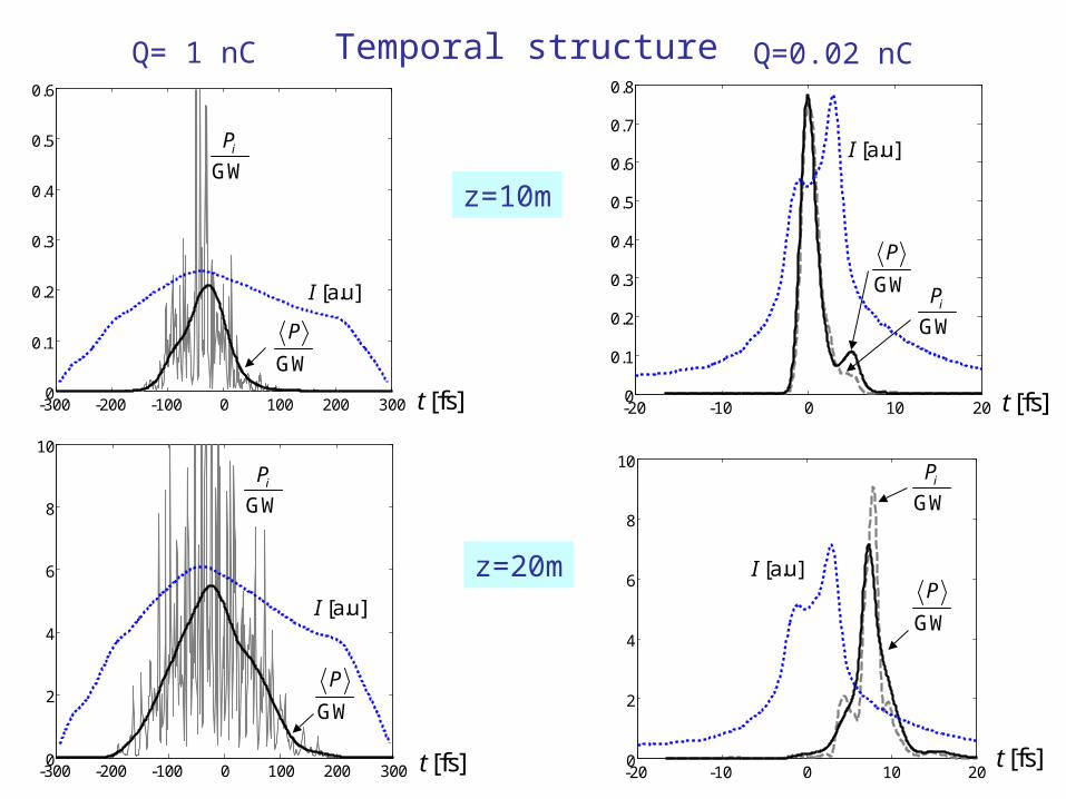
Temporal structure

[fs]t

Q= 1 nC Q=0.02 nC

[a.u]I

[a.u]I

[a.u]I

GWiP

GW

P

[fs]t

[fs]t

[fs]t

z=10m

z=20m[a.u]I

GWiP

GW

P

GWiP

GW

P

GWiPGW

P

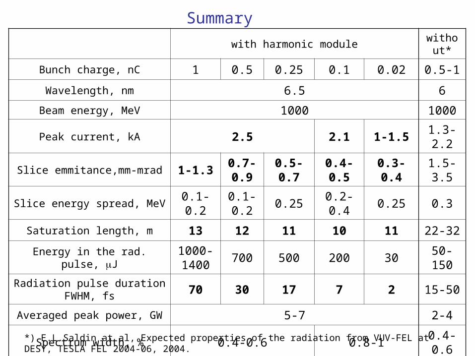
Summarywith harmonic module without*

Bunch charge, nC 1 0.5 0.25 0.1 0.02 0.5-1

Wavelength, nm 6.5 6

Beam energy, MeV 1000 1000

Peak current, kA 2.5 2.1 1-1.5 1.3-2.2

Slice emmitance,mm-mrad 1-1.30.7-0.9

0.5-0.7 0.4-0.5 0.3-0.4 1.5-3.5

Slice energy spread, MeV 0.1-0.20.1-0.2

0.25 0.2-0.4 0.25 0.3

Saturation length, m 13 12 11 10 11 22-32

Energy in the rad. pulse, J1000-1400

700 500 200 30 50-150

Radiation pulse duration FWHM, fs 70 30 17 7 2 15-50

Averaged peak power, GW 5-7 2-4

Spectrum width, % 0.4-0.6 0.8-1 0.4-0.6

Coherence time, fs 4-5 - - -

*) E.L.Saldin at al, Expected properties of the radiation from VUV-FEL at DESY, TESLA FEL 2004-06, 2004.

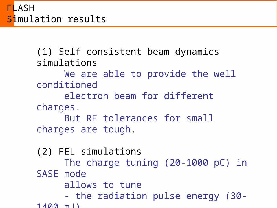
FLASHSimulation results

(1) Self consistent beam dynamics simulations We are able to provide the well conditioned electron beam for different charges. But RF tolerances for small charges are tough.

(2) FEL simulationsThe charge tuning (20-1000 pC) in SASE mode allows to tune - the radiation pulse energy (30-1400 mJ) - the pulse width (FWHM 3-70 fs).