Embed Size (px)
Citation preview
CER
N-T
HES
IS-2
011-
138
26/0
9/20
11
Beam-Beam Interaction Studies atLHC
Master Thesis
Michaela Schaumann
RWTH Aachen UniversitySupervisor: Prof. Dr. Achim Stahl
CERNEuropean Organization for Nuclear ResearchSupervisor: Dr. Reyes Alemany Fernandez
Abstract
The beam-beam force is one of the most important limiting factors in the performanceof a collider, mainly in the delivered luminosity. Therefore, it is essential to measurethe effects in LHC. Moreover, adequate understanding of LHC beam-beam interactionis of crucial importance in the design phases of the LHC luminosity upgrade. Dueto the complexity of this topic the work presented in this thesis concentrates on thebeam-beam tune shift and orbit effects.
The study of the Linear Coherent Beam-Beam Parameter at the LHC has beendetermined with head-on collisions with small number of bunches at injection energy(450 GeV). For high bunch intensities the beam-beam force is strong enough to expectorbit effects if the two beams do not collide head-on but with a crossing angle or witha given offset. As a consequence the closed orbit changes. The closed orbit of anunperturbed machine with respect to a machine where the beam-beam force becomesmore and more important has been studied and the results are as well presented.
September 2011

Contents
Contents
1 Theoretical Motivation 51.1 Luminosity and the Geometry of a Particle Collider . . . . . . . . . . . 61.2 Fields and Forces . . . . . . . . . . . . . . . . . . . . . . . . . . . . . . 8
1.2.1 Beam-Beam Force . . . . . . . . . . . . . . . . . . . . . . . . . 81.2.2 Linear Beam-Beam Tune Shift . . . . . . . . . . . . . . . . . . . 11
1.3 Resulting Effects . . . . . . . . . . . . . . . . . . . . . . . . . . . . . . 151.3.1 Incoherent Effects . . . . . . . . . . . . . . . . . . . . . . . . . . 151.3.2 Coherent Effects . . . . . . . . . . . . . . . . . . . . . . . . . . 15
1.4 Long-Range Interactions . . . . . . . . . . . . . . . . . . . . . . . . . . 16
2 The Large Hadron Collider 212.1 Physics Motivation . . . . . . . . . . . . . . . . . . . . . . . . . . . . . 212.2 The Machine . . . . . . . . . . . . . . . . . . . . . . . . . . . . . . . . 22
2.2.1 Injection System . . . . . . . . . . . . . . . . . . . . . . . . . . 222.2.2 Magnets . . . . . . . . . . . . . . . . . . . . . . . . . . . . . . . 242.2.3 Closed Orbit Correctors . . . . . . . . . . . . . . . . . . . . . . 282.2.4 Cryogenics and Superconductivity . . . . . . . . . . . . . . . . . 282.2.5 Radio Frequency Cavities . . . . . . . . . . . . . . . . . . . . . 302.2.6 Collimator System . . . . . . . . . . . . . . . . . . . . . . . . . 302.2.7 Beam Dump . . . . . . . . . . . . . . . . . . . . . . . . . . . . . 30
2.3 Measurement Devices for Beam Dynamics . . . . . . . . . . . . . . . . 312.3.1 Fast Beam Current Transformer (FBCT) . . . . . . . . . . . . . 312.3.2 Beam Position Monitor (BPM) . . . . . . . . . . . . . . . . . . 332.3.3 Wire Scanner . . . . . . . . . . . . . . . . . . . . . . . . . . . . 352.3.4 Beam Synchrotron Radiation Telescope (BSRT) . . . . . . . . . 372.3.5 Schottky Pick-Up . . . . . . . . . . . . . . . . . . . . . . . . . . 402.3.6 Machine Luminosity Monitors (BRAN) . . . . . . . . . . . . . . 44
3 Linear Coherent Beam-Beam Parameter 453.1 Nominal and Current Operational Situation . . . . . . . . . . . . . . . 463.2 Experimental Conditions . . . . . . . . . . . . . . . . . . . . . . . . . . 473.3 Analysis of MD Data from 30/06/2011 . . . . . . . . . . . . . . . . . . 48
3.3.1 Observations . . . . . . . . . . . . . . . . . . . . . . . . . . . . 493.3.2 Absolute Value of the Emittance . . . . . . . . . . . . . . . . . 513.3.3 Linear Coherent Beam-Beam Parameter . . . . . . . . . . . . . 533.3.4 Tune Shift from Tune Measurements . . . . . . . . . . . . . . . 56
3
Contents
3.3.5 Conclusion for Fill 1911 . . . . . . . . . . . . . . . . . . . . . . 583.4 Analysis of Further Data . . . . . . . . . . . . . . . . . . . . . . . . . . 593.5 Conclusion . . . . . . . . . . . . . . . . . . . . . . . . . . . . . . . . . . 60
4 Orbit Effects 634.1 Long-Range Beam-Beam Kick . . . . . . . . . . . . . . . . . . . . . . . 644.2 Orbit Effects due to Bunch-by-Bunch Differences . . . . . . . . . . . . 71
4.2.1 Simulations . . . . . . . . . . . . . . . . . . . . . . . . . . . . . 714.2.2 Beam Position Monitors . . . . . . . . . . . . . . . . . . . . . . 754.2.3 ATLAS Luminous Region Reconstruction . . . . . . . . . . . . . 764.2.4 Luminosity Optimization . . . . . . . . . . . . . . . . . . . . . . 80
5 Conclusion 83
6 Acknowledgement 85
4
Theoretical Motivation
1 Theoretical Motivation
The performance of a particle collider is quantified by the energy available for the pro-duction of new physics events and by the luminosity. The required large center of massenergy can only be provided with colliding beams where little or no energy is lost inthe motion of the center of mass system, like it would be the case for beam-on-targetexperiments. Therefore two counter rotating beams are injected into a circular accel-erator or storage ring and are brought into collisions once accelerated to the maximumenergy. The beams are now interacting with each other in two different ways:
1. High energy collisions between two particles.
2. Distortion of the beam by electromagnetic forces.
The first interaction is the aim of building a particle collider and therefore highlywanted. The outcome of these high energy collisions will be measured in the detectors.
On the other hand, the particles in the beam will be distorted by crossing the op-posite beam, since one beam is a collection of charged particles and thus represents anelectromagnetic potential for the other beam. Hence, a charged beam will exert forceson itself (space charge) and on the other beam (beam-beam effects). Unfortunatelythese two effects go together and cannot be separated. Typically 0.001% (or less) ofthe particles collide and 99.999% are distorted [1].
These interactions can be very strong and occur whenever the two beams share acommon beam pipe. This can either be directly at the interaction points (IP), wherethe beams are brought into collisions on purpose, or in the interaction region (IR) toboth sides of the IP, where the two beams are already sharing the same beam pipe inorder to prepare for the collisions in the IP. All interactions happening not directly atthe IP are parasitic encounters and undesirable.
The beam-beam force is one of the most important and limiting factors in the per-formance of a particle collider. Many beam parameters are affected, resulting in a widespectrum of effects for the beam dynamics like, tune shift with the risk of crossing res-onances, dynamic aperture reduction due to distortion of the phase space, orbit effects,etc.
From a theoretical point of view, the easiest way to study the beam-beam effectsis to look at the changes the forces of one beam exert to the behaviour of a singletest particle crossing this beam. The beam will act on that test particle like a strongnon-linear electromagnetic lens. The test particle will be affected by the beam, butthe effect the single particle has on the opposite beam can be neglected. Nevertheless,in a real particle collider a beam is rather colliding with an ensemble of particles thanwith a single one, therefore collective effects have to be taken into account. Now the
5
Theoretical Motivation
one beam will disturb every single particle in the other beam as mentioned before, butdue to the different positions the particles have with respect to the center of the beamthey are crossing, they see a different particle distribution and therefore each particleis affected by a different force. On the other hand, these effects must be applied viceversa to the other beam. It acts as an electromagnetic lens to the first beam, as wellas it exerts forces to the opposite beam in the same way but depending on its ownparticle distribution [2].
Moreover, as a result of the interaction the distribution in both beams can change,so that the force becomes time dependent. A self-consistent treatment is necessary insimulations of the beam-beam force, i.e. since the forces change dynamically, they haveto be recalculated after each crossing.
To study beam-beam effects the force needs to be known. To predict a model,concepts of non-linear dynamics and multiple-particle dynamics must be applied. An-alytical models and simulation techniques were well developed in the last 10 years andtheir predicting power is improving, but the LHC represents a new and unknown regimefor what concerns beam-beam interactions. Present models do not have the predictivepower needed for such an accelerator layout. Even if a general, qualitative understand-ing of beam-beam interactions is available, a quantitative and detailed study for thecase of multiple bunch beams and multiple beam-beam interactions does not exist sofar [3].
Also different beam parameters for both beams (which can also change dynamicallydue to the interaction) can have very detrimental effects on the beam. This results ina wide spectrum of effects for the beam dynamics. Due to the complexity of this topicnot all effects can be discussed in detail in the scope of this thesis, the analysis herewill concentrate on a few particular effects.
As said before, the beam-beam force is one of the most important limiting factors inthe performance of a particle collider. They become especially important for high den-sity beams, i.e. high intensity and/or small beam sizes to achieve high luminosities.Therefore, it is essential to measure the effects at LHC. Moreover, adequate under-standing of LHC beam-beam interaction is of crucial importance in the design phasesof the LHC luminosity upgrade.
1.1 Luminosity and the Geometry of a Particle
Collider
Besides the beam energy the number of useful interactions (events) is as well a veryimportant parameter, especially when rare events with a small production cross sec-tion are studied. The quantity that measures the ability of a particle accelerator toproduce the required number of interactions is called luminosity and represents theproportionality factor between the number of produced events per unit of time, dR/dt,and the production cross-section of the considered reaction, σp:
6
Theoretical Motivation
dR
dt= L× σp (1.1)
The luminosity is calculated from the beam parameters and is given in units ofcm−2s−1. In the specific case of a circular collider and when the particle density dis-tribution can be approximated to a Gaussian, the luminosity of two beams collidingexactly head-on is given by:
L =N1N2fNb
2π√σ2x1 + σ2
x2
√σ2y1 + σ2
y2
(1.2)
where N1 and N2 are the two colliding bunch intensities, f is the revolution frequencyof the bunches in the ring, Nb the number of bunches per beam, and σxi and σyi arethe transversal beam-sizes in the horizontal and vertical direction, respectively. In theapproximation of equal distributions for both beams σx1 = σx2 and σy1 = σy2, Equation1.2 simplifies to
L =N1N2fNb
4πσxσy(1.3)
If the interaction is not exactly head-on the luminosity is reduced by a factor S,the so-called luminosity reduction factor. It represents the geometrical overlap of thetwo particle distributions, which can be equal to one, when the two distributions areperfectly overlapping, or smaller than one in case of collisions with a crossing angle,offsets, hourglass effect, non-Gaussian beam profile and/or non-zero dispersion at thecollision point [4].
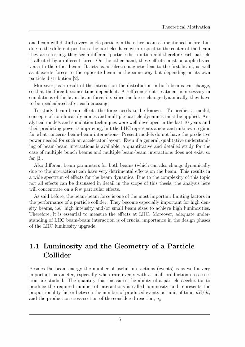
Since the luminosity is proportional to the number of bunches Nb, it is desirable tooperate a collider with as many bunches as possible to get the highest luminosity. Ina single ring collider such as LEP, the operation with k bunches leads to 2 · k collisionpoints. When k is a large number, most of them are unwanted and must be avoidedto reduce the perturbation due to the beam-beam effects. On the other hand, theLHC uses two separated beam-pipes, since two equally charged proton beams counterrotate around the ring. Therefore, the two beams need to be brought together into acommon vacuum chamber to make them collide at the interaction points. Figure 1.1shows schematically the beams crossing in the horizontal plane at the IP with a givencrossing angle achieved by an arrangement of separation and recombination magnetsaround the interaction region [2].
The beams travel in a shared beam-pipe for more than 120 m to adjust the bunchesfor the crossing and to separate them again into their own pipes afterwards. Undernominal conditions the distance between the bunches is only 25 ns, therefore they willmeet in the whole region and not only in the foreseen interaction point. Out of thebunch spacing and the length of the interaction region it can easily be calculated
7
Theoretical Motivation
D1 IT
IP
D2
Figure 1.1: Cross over between innerand outer vacuum chamber in the LHC(schematic) [2]. IT = inner tripletmagnets, D1 and D2 = separation-recombination dipoles.
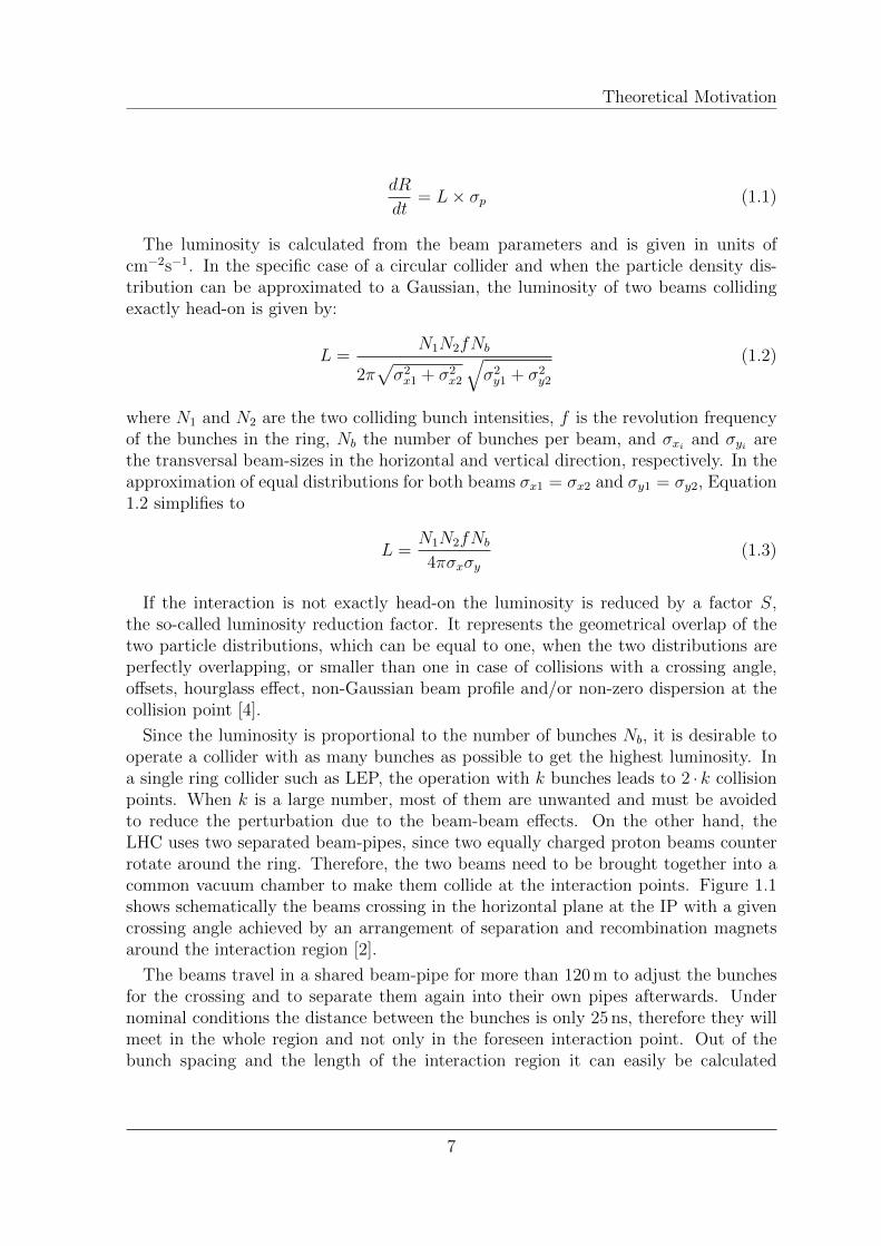
Figure 1.2: Head-on and long-range in-teractions in a LHC interaction point[2].
that around 30 bunch encounters in one of the four LHC interaction regions can beexpected, i.e. in total 120 interactions. Except for the interactions in the IP, the restare undesirable and they must be avoided to not unnecessarily disturb the beam. Theinsertion of a crossing angle eliminates all unwanted head-on collisions but leads to theso-called long-range interactions as illustrated in Figure 1.2.
The long-range interactions imply that the bunches still feel the electromagneticforces from the bunches of the opposite beam. When the separation is large enough,these long-range encounters should be weak. In nominal LHC the bunches collide ata small crossing angle of 285µrad. The typical separation between the two beams isbetween 7 and 10 in units of the beam-size of the opposing beam [2]. Therefore, long-range interactions destroy the beam much less than head-on interactions, but due totheir large number and some particular properties they require careful studies.
From now on it will be distinguished between these two regimes of beam-beam in-teractions:
• Head-on interactions (HO), short range electromagnetic interactions.
• Long-range interactions (LR), long-range electromagnetic interactions.
1.2 Fields and Forces
1.2.1 Beam-Beam Force
To calculate the effect one beam has on a particle in the opposite beam the electro-magnetic fields ( ~E, ~B) of the beam with a particle density distribution ρ(x, y, z) needsto be known. In the rest frame of the moving beam the fields are electrostatic and theycan be calculated via the electrostatic potential.
Any charged particle density distribution ρ generates an electrostatic field ( ~E ′, ~B′ ≡ 0):
~∇ ~E ′ = ρ
ε0(1.4)
8
Theoretical Motivation
The electrostatic field can be calculated from the divergence of a potential
~E ′ = −~∇Φ(x, y, z) (1.5)
Bringing 1.5 into 1.4 the following expressions are obtained:
− ~∇( ~∇Φ) =ρ
ε0=⇒ ∆Φ = − ρ
ε0(1.6)
where ~∇ · ~∇ = ∆ is used. Equation 1.6 is known as the Poisson equation. Knowing thecharged density distribution ρ, the potential can be obtained and from the potentialthe electrostatic fields from 1.5.
One particular solution of the Poisson equation is [5]
Φ(x, y, z) =1
4πε0
∫ρ(x, y, z)dV
R(1.7)
In case of beams with (2D) Gaussian charged particle density distributions
ρ(x, y) =NZ1e
2πσxσyexp
(− x2
2σ2x
− y2
2σ2y
)(1.8)
with N particles of the charge q = Z1e the potential becomes [2]
U(x, y, σx, σy) =NZ1e
4πε0
∫ ∞0
exp(− x2
2σ2x+q− y2
2σ2y+q
)√
(2σ2x + q)(2σ2
y + q)dq (1.9)
As said before, once the potential is known, one can get the electrostatic field ~E ′.Since the beam is moving the field has to be Lorentz transformed into the movingframe:
E‖ = E ′‖, E⊥ = γ ·E ′⊥ (1.10)
The Lorentz force ~F on a particle with charge q = Z2e can be calculated with
~B = ~β × ~E/c (1.11)
~F = q( ~E + ~βc× ~B) (1.12)
where γ = 1/√
1− β2 is the Lorentz factor and ~β = ~v/c is the relativistic beta.
For very relativistic particles (β ≈ 1) and under the assumptions of round beams(σx = σy = σ, which is a good assumption for a hadron collider) and Z1 = Z2 = 1 theresulting Lorentz force has only a radial component, i.e. depends only on the distancer from the bunch center (where r2 = x2 + y2), since only the components Er and BΦ
9
Theoretical Motivation
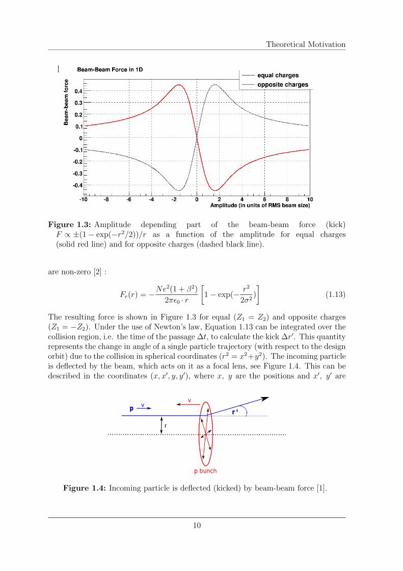
Figure 1.3: Amplitude depending part of the beam-beam force (kick)F ∝ ±(1− exp(−r2/2))/r as a function of the amplitude for equal charges(solid red line) and for opposite charges (dashed black line).
are non-zero [2] :
Fr(r) = −Ne2(1 + β2)
2πε0 · r
[1− exp(− r2
2σ2)
](1.13)
The resulting force is shown in Figure 1.3 for equal (Z1 = Z2) and opposite charges(Z1 = −Z2). Under the use of Newton’s law, Equation 1.13 can be integrated over thecollision region, i.e. the time of the passage ∆t, to calculate the kick ∆r′. This quantityrepresents the change in angle of a single particle trajectory (with respect to the designorbit) due to the collision in spherical coordinates (r2 = x2+y2). The incoming particleis deflected by the beam, which acts on it as a focal lens, see Figure 1.4. This can bedescribed in the coordinates (x, x′, y, y′), where x, y are the positions and x′, y′ are
Figure 1.4: Incoming particle is deflected (kicked) by beam-beam force [1].
10
Theoretical Motivation
the angles of the particle with respect to the design orbit. The deflections ∆x′ and ∆y′
give the angles by which the particle is deflected during the passage, i.e. the kick dueto the beam-beam force:
∆r′ = −2Nr0
γ·r
r2·[1− exp(− r2
2σ2)
](1.14)
1.2.2 Linear Beam-Beam Tune Shift
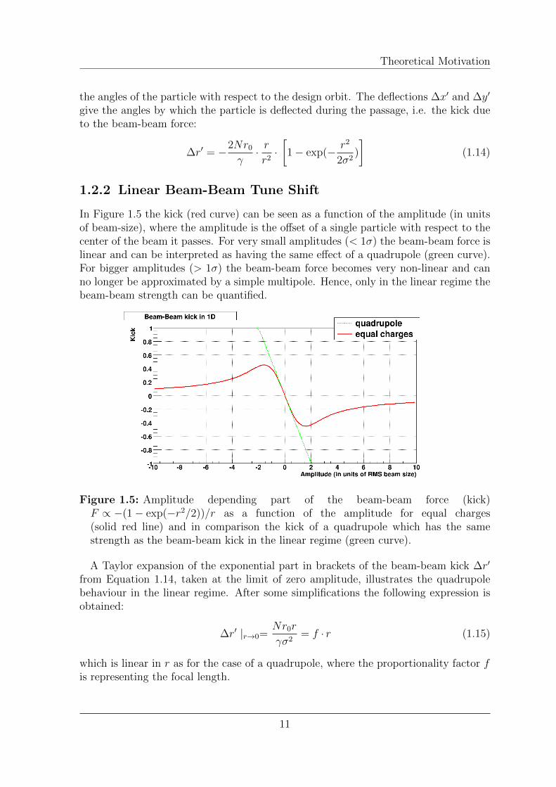
In Figure 1.5 the kick (red curve) can be seen as a function of the amplitude (in unitsof beam-size), where the amplitude is the offset of a single particle with respect to thecenter of the beam it passes. For very small amplitudes (< 1σ) the beam-beam force islinear and can be interpreted as having the same effect of a quadrupole (green curve).For bigger amplitudes (> 1σ) the beam-beam force becomes very non-linear and canno longer be approximated by a simple multipole. Hence, only in the linear regime thebeam-beam strength can be quantified.
Figure 1.5: Amplitude depending part of the beam-beam force (kick)F ∝ −(1− exp(−r2/2))/r as a function of the amplitude for equal charges(solid red line) and in comparison the kick of a quadrupole which has the samestrength as the beam-beam kick in the linear regime (green curve).
A Taylor expansion of the exponential part in brackets of the beam-beam kick ∆r′
from Equation 1.14, taken at the limit of zero amplitude, illustrates the quadrupolebehaviour in the linear regime. After some simplifications the following expression isobtained:
∆r′ |r→0=Nr0r
γσ2= f · r (1.15)
which is linear in r as for the case of a quadrupole, where the proportionality factor fis representing the focal length.
11

Theoretical Motivation
The effect of this behaviour on the beam can be understood by looking at the kickgiven by a normal quadrupole. The horizontal kick x′ of a quadrupole can be seen asa change in angle which can be estimated via
x′ =l
ρ(1.16)
where l is the path length the particle travels in the quadrupole field and ρ is thebending radius of the deviation curve inside the magnet. Multiplying by 1 = B/Band replacing B = gx in the numerator, where g = k · (p/q) is the gradient of thequadrupole field, and the beam rigidity Bρ = p/q in the denominator, Equation 1.16can be rewritten as
x′ =B · lB · ρ
=gx · lp/q
=k(p/q) ·x · l
p/q= kl ·x = f ·x (1.17)
here f is equal to the inverse of the focal length F = 1/kl. Thus, the same linearbehaviour as for the linear beam-beam force is obtained.
But since no quadrupole can be built with a perfect field, small errors ∆k in the fieldstrength k will occur. Such an error leads to a change in tune (tune shift)
∆Q =1
4π
∫∆kβds (1.18)
where the integral has to be carried out over the length of the considered quadrupoleand with β as the beta-function at its position. As seen before, the quadrupole strengthcan be expressed in terms of the field gradient:
g =dB
dx(1.19)
From this it follows that a change in tune ∆Q is proportional to the derivative of themagnetic field. In conclusion, the focal length of a quadrupole relates to the experi-enced tune shift which is proportional to the derivative of the applied force.
With this in mind the linear beam-beam parameter ξ for head-on interactions ofround beams with β∗ = β∗x = β∗y can be derived:
ξ =Nr0β
∗
4πγrelσ2(1.20)
where N is the bunch intensity, r0 = e2/4πε0mc2 is the classical particle radius, β∗
is the optical amplitude function (β-function) of the particle at the interaction point,γrel = E/m0 is the relativistic γ describing the fraction between the energy and therest mass of the particle and σ describes the transverse beam size at the interactionpoint.
12
Theoretical Motivation
The beam-beam parameter can be generalized for the case of non-round beams, butGaussian particle distributions in both planes:
ξx,y =Nr0β
∗x,y
2πγrelσx,y(σx + σy)(1.21)
For small values of ξ and a tune far enough away from linear resonances this pa-rameter is proportional to the linear tune shift ∆Qbb due to beam-beam interactions.The change in tune due to beam-beam interactions is to be added to the unperturbedtune Q set by the main quadrupoles in the machine. This perturbation due to head-oncollisions occurs in both planes and can be focusing or defocusing, depending on thecharges of the colliding particles. If the beams consist of opposite charged particles(e.g colliding electron-positron or proton-antiproton beams) the effect is focusing, byconsidering equally charged beams, as the two colliding proton beams in LHC, oneobtains a defocusing effect, which leads to a decrease in tune.
One can visualize this defocusing effect by thinking of the repulsion between twoequally charged particles. The beams will repulse each other, resulting in a kick whichhas the same direction as one of a defocusing quadrupole. Vice versa, from the attrac-tion between two opposite charges a focusing effect follows. In the linear regime thebeam-beam force is focusing in both planes. However, a quadrupole is focusing in theone and defocusing in the other plane.
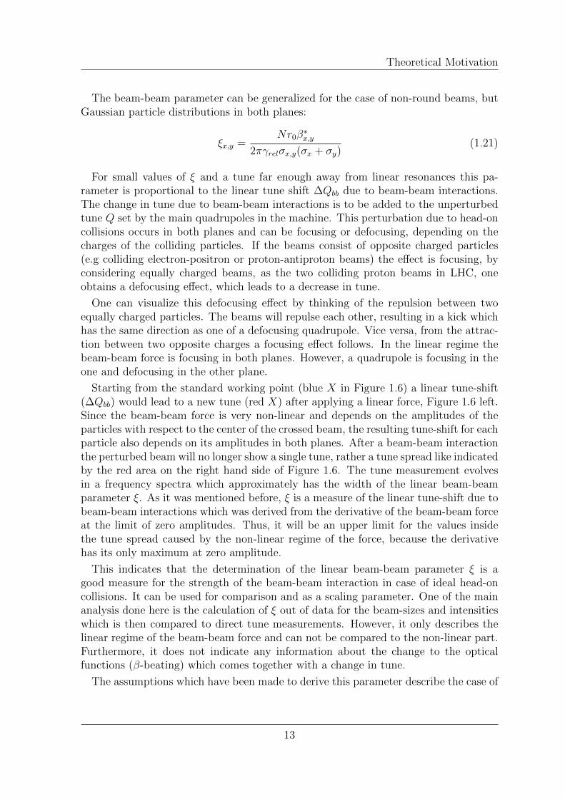
Starting from the standard working point (blue X in Figure 1.6) a linear tune-shift(∆Qbb) would lead to a new tune (red X) after applying a linear force, Figure 1.6 left.Since the beam-beam force is very non-linear and depends on the amplitudes of theparticles with respect to the center of the crossed beam, the resulting tune-shift for eachparticle also depends on its amplitudes in both planes. After a beam-beam interactionthe perturbed beam will no longer show a single tune, rather a tune spread like indicatedby the red area on the right hand side of Figure 1.6. The tune measurement evolvesin a frequency spectra which approximately has the width of the linear beam-beamparameter ξ. As it was mentioned before, ξ is a measure of the linear tune-shift due tobeam-beam interactions which was derived from the derivative of the beam-beam forceat the limit of zero amplitudes. Thus, it will be an upper limit for the values insidethe tune spread caused by the non-linear regime of the force, because the derivativehas its only maximum at zero amplitude.
This indicates that the determination of the linear beam-beam parameter ξ is agood measure for the strength of the beam-beam interaction in case of ideal head-oncollisions. It can be used for comparison and as a scaling parameter. One of the mainanalysis done here is the calculation of ξ out of data for the beam-sizes and intensitieswhich is then compared to direct tune measurements. However, it only describes thelinear regime of the beam-beam force and can not be compared to the non-linear part.Furthermore, it does not indicate any information about the change to the opticalfunctions (β-beating) which comes together with a change in tune.
The assumptions which have been made to derive this parameter describe the case of
13
Theoretical Motivation
Figure 1.6: Left: linear tune-shift caused by a linear force. Right: footprint of thetune spread caused by a non-linear beam-beam force. The blue X indicates theposition of the unperturbed working-point, the red X/bordered region representsthe point/area in which the single particle tunes are located after a head-on collisionwith the opposite beam when a linear/non-linear force is exerted [1].
the LHC very well. The LHC is a high energy hadron collider in which round Gaussianbeams are in general a good approximation. On the other hand, the assumptionsmade above would not describe the conditions for instance in LEP very well. Evenif in LEP the particles are accelerated to ultra relativistic energies, the beams arevery asymmetric in both transversal planes. The horizontal beam-size is much biggerthan the vertical one, because the beams are deviated by the dipole-magnets in thehorizontal plane, the beam profile in this plane increases due to synchrotron radiation.
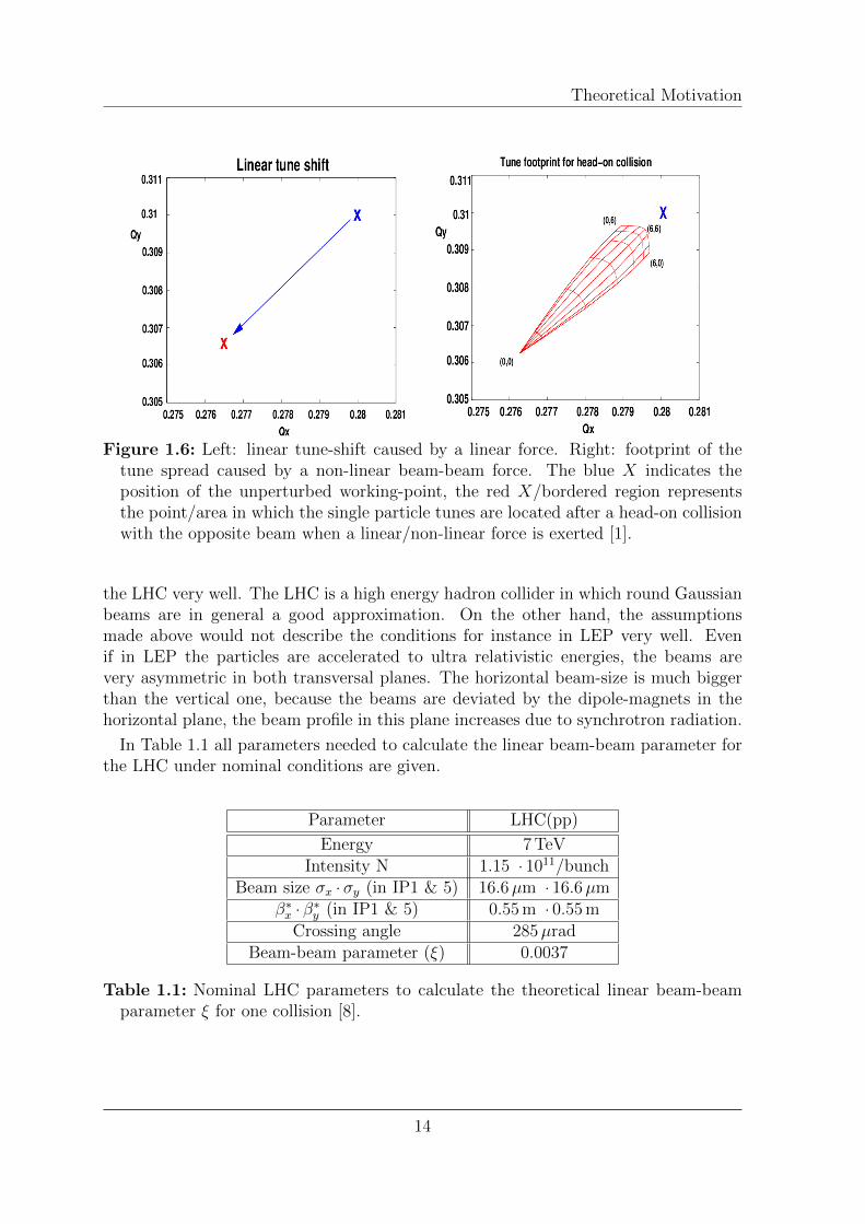
In Table 1.1 all parameters needed to calculate the linear beam-beam parameter forthe LHC under nominal conditions are given.
Parameter LHC(pp)
Energy 7 TeVIntensity N 1.15 · 1011/bunch
Beam size σx ·σy (in IP1 & 5) 16.6µm · 16.6µmβ∗x · β∗y (in IP1 & 5) 0.55 m · 0.55 m
Crossing angle 285µradBeam-beam parameter (ξ) 0.0037
Table 1.1: Nominal LHC parameters to calculate the theoretical linear beam-beamparameter ξ for one collision [8].
14
Theoretical Motivation
1.3 Resulting Effects
In this section, the effects of the fields and forces discussed in Section 1.2 on the beamdynamics are summarized.
1.3.1 Incoherent Effects
Incoherent effects are effects on single particles. They can not be measured directly,but their evaluation is done by simulations to help in the understanding of the data.
However, as discussed above, all single particles in one beam will be affected by thebeam-beam force exert by the opposite beam. The beam will act on each single particleof the counter rotating beam as a complex, static electromagnetic lens. It should beclear that the exerted force is very non-linear and highly depending on the amplitude,therefore one has to expect all effects known from non-linear beam dynamics, dependingon the complexity of the lens.As the main effects of beam-beam interactions which will deviate the particles fromtheir linear and stable dynamics one has to expect the following [3]:
• Non-linear detuning and excitation of resonances.
• Transverse phase space modification and beam blow up.
• Unstable and/or irregular motion
• Dynamic aperture reduction, bad lifetime and particle losses.
• Dynamic beta effects.
1.3.2 Coherent Effects
Coherent beam-beam effects are collective and organized motions of many particlesor bunches. They arise from the force which an exciting bunch exerts on a wholetest bunch during beam-beam collisions. A coherent kick is seen by the entire bunch,which is the difference to the incoherent kick, where only the effect on a single particleis considered. By coherent motion of bunches, the collective behaviour of all particlesin a bunch is meant.
The calculation of the coherent force between two charged, Gaussian particle dis-tributions, is done as for the incoherent case in Chapter 1.2. The computation of thecoherent kick requires the integration of the individual incoherent kicks of all test par-ticles over the bunch distribution. Analogue to the incoherent case, only by taking thebunch barycentres (X, Y ) as the coordinates of the bunches (instead of the positions ofthe single particles x and y) this leads, in the limit of exact head-on collisions (r → 0),to a coherent kick given by the expression:
∆r′ |r→0=Nr0r
2γσ2= F · r (1.22)
15
Theoretical Motivation
Where the kick can again be represented by a quadrupole with an inverse focal length ofF = f/2, being only half the value of the incoherent one, f . This quantity again relatesto a tune change and, like in the incoherent case, a coherent beam-beam parameter Ξfor r → 0 can be defined. For the case of elliptical Gaussian bunches it is of the form
ΞX,Y =Nr0β
∗X,Y
4πγσX,Y (σX + σY )(1.23)
For round beams (σX = σY ) it simplifies to
ΞX,Y =Nr0β
∗X,Y
8πγσ2=
1
2ξX,Y (1.24)
For small amplitudes (r << σ) the overall effect on the entire beam is therefore onlyhalf the effect on a single particle. At large distances this is no longer true, because thebunches appear to each other as a point like source and the force can be approximatedwith the effect on a single particle [3].
Due to the beam-beam interactions the beams can couple through the beam-beamforce and develop a collective behaviour. Therefore the beam will not only show per-turbed single particle dynamics but also new coherent effects, like
• Orbit effects
• Coherent oscillating modes
• Multi Bunch coupling
This thesis will focus on the analysis of coherent effects, and in particular on orbiteffects and the coherent tune shift.
1.4 Long-Range Interactions
Long-range interactions break the symmetry between the planes and can lead tostronger excitation of resonances. They mostly affect particles at large amplitudesand they cause effects on the tune and closed orbit, e.g. PACMAN-effect.
In ATLAS (IP1) and ALICE (IP2) the beams are colliding with a crossing angle inthe vertical plane and in CMS (IP5) and LHCb (IP8) in the horizontal plane. Theorthogonal plane is called separation plane, since here the beams can be separated toreduce or avoid collisions, without touching the crossing angle in the other plane. InIP1 and 5 the beams collide head-on without separation, but in IP2 and 8 a sepa-ration is applied in the orthogonal plane to the crossing angle plane, i.e. the beamssee long-range interactions in both planes in IP2 and 8, whereas in IP1 and 5 thebeams only suffer from long-range encounters in the crossing plane. The alternatingcrossing scheme is used to compensate for the effect of long-range interactions. Thefunctionality can be easily understood by considering for instance a normal quadrupolefocusing in the horizontal plane. It is well known that this quadrupole will act as a
16
Theoretical Motivation
defocusing element in the vertical plane, where an analogue behaviour of the long-rangeinteractions can be found.
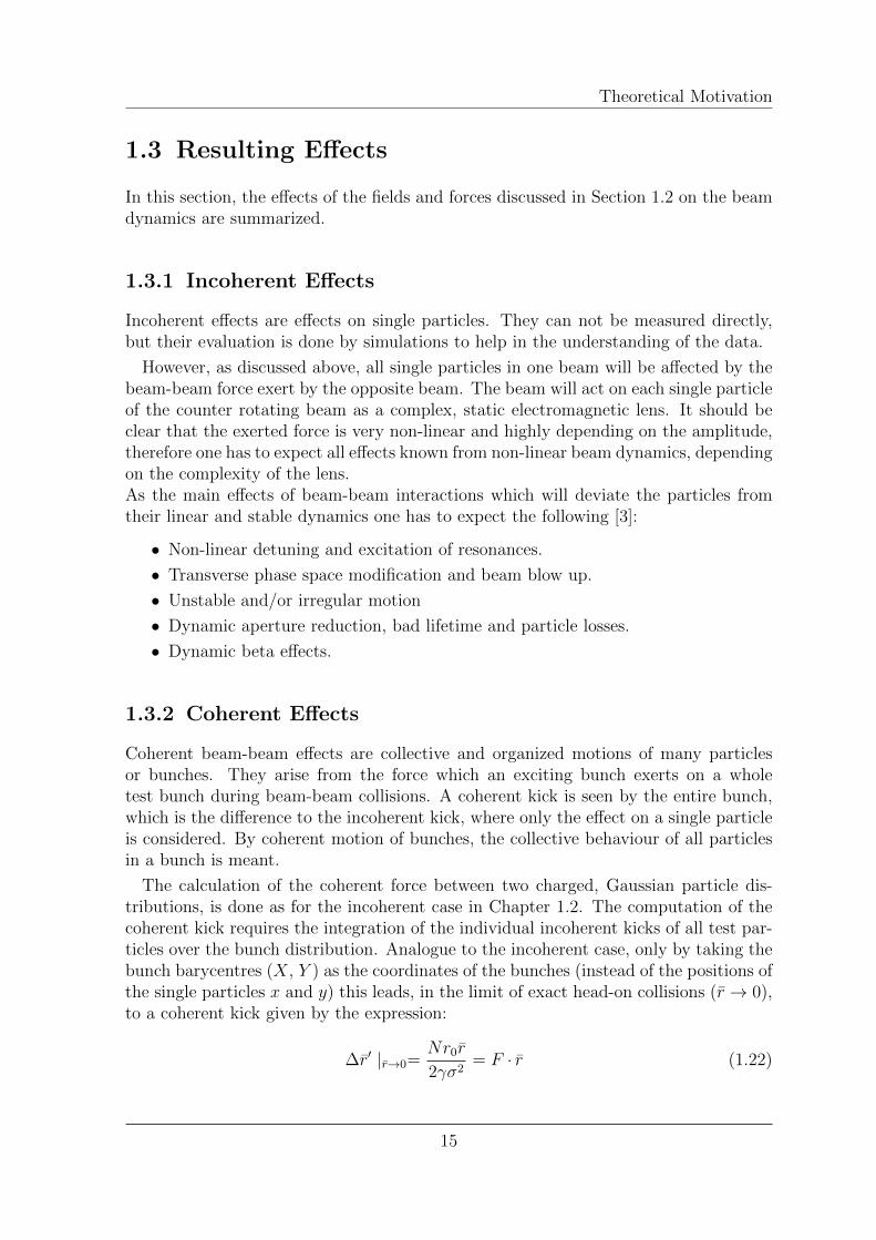
The tune shift due to long-range interactions has the opposite sign compared tothat caused by head-on interactions, see Figure 1.7. For small amplitude particles,represented with a blue spot, the effect can be approximated as a defocusing quadrupole(for equally charged beams). But if particles at larger amplitudes (r > 2σ, yellow spot)are considered, the local slope of the kick due to the beam-beam interactions changessign. Thus, the particles are kicked in the opposite direction and are focused insteadof defocused.
Figure 1.7: The opposite sign of the tune shift due to long-range interactions, arisesfrom the opposite slope of the beam-beam kick at larger amplitudes [1].
If the beams are crossing in the vertical plane in IP1, the long-range effects will focusthe beams in the vertical (since here the bunches are separated by the crossing angle)and defocus them in the horizontal plane (since here they collide head-on with zeroseparation). Arriving at IP5, they cross in the horizontal plane, which leads to a swapof the focusing due to beam-beam interactions with respect to IP1 (focus horizontallyand defocus vertically). This entails the same behaviour as a FoDo-cell and results ina compensation of the undesired effects to the tune.
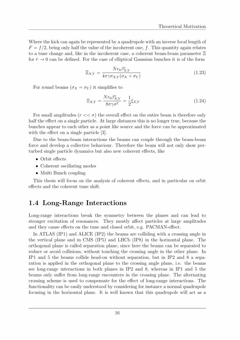
It can easily be seen that the effects caused by the long-range interactions depend onthe size of the separation dsep. The closer the bunches are, the stronger the field theyfeel, thus the kick becomes stronger (Figure 1.8). The number of long-range interactionsdepends on the spacing between bunches and the length of the common vacuum pipe.However, it can be calculated that the resulting tune shift for one particular interactionfollows (for large enough dsep) the proportionality relation [2]
∆QLR ∝ −N
d2sep
(1.25)
17
Theoretical Motivation
Figure 1.8: Long-range interactions depend on the separation dsep [1].
As mentioned before, the tune shift is proportional to the derivative of the appliedforce, hence it can be seen from Equation 1.25, that for well separated beams (d >>σ) the force (kick) has an amplitude independent contribution, which changes theorbit. The whole bunch sees a kick as an entity (coherent kick), which can excitecoherent dipole oscillations. Moreover, all bunches couple because each bunch seesmany opposing bunches and therefore many coherent modes are possible. In dailyoperation the separation, due to the crossing angle, between two bunches in LHC ismaximal around 10 in units of beam-size, thus it is not unusual to reach the regimewhere the beam-beam kick changes its sign.
Furthermore, more problems must be expected for small crossing angles. In thiscases the interactions become stronger, since the separation decreases. For very smallseparations particles become unstable and get lost.
PACMAN-Effect
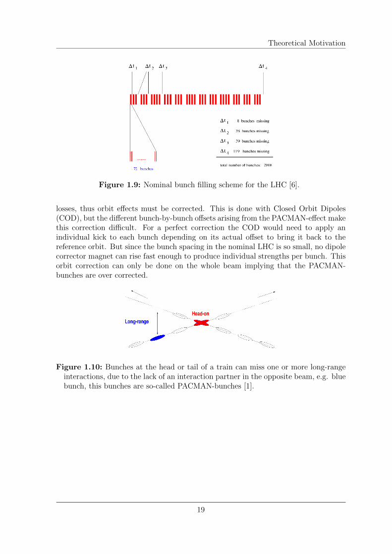
For high luminosity operation, the LHC is filled with 39 batches of 72 bunches with a25 ns spacing in each batch, this sums up to 2808 bunches. But from the length of thering one can calculate that for a spacing of 25 ns 3564 bunch positions are possible, i.e.this scheme contains 756 gaps between the batches, see Figure 1.9.
The gaps are unavoidable and necessary to give the SPS (Super Proton Synchrotron)and LHC kickers time to rise to inject the next batches from the PS (Proton Syn-chrotron) into the SPS and later on into the LHC [7]. These gaps cause the so-calledPACMAN-effect. PACMAN-bunches are the bunches which see fewer unwanted long-range interactions in total, because they are located at the head or tail of a bunchtrain and they do not have an interaction partner from the arriving or leaving counterrotating beam, see Figure 1.10. The result is a left-right asymmetry which leads toa maximum of 120 and a minimum of 40 long-range collisions for different bunches.Bunches at different positions in a bunch train therefore experience different orbit kicks,which results in bunch-by-bunch differences in the offset with respect to the referenceorbit. PACMAN-bunches have a different offset than the bunches in the middle of abunch train which experience all possible long-range interactions.
Due to the orbit changes the lattice properties also change, which can cause particle
18
Theoretical Motivation
Figure 1.9: Nominal bunch filling scheme for the LHC [6].
losses, thus orbit effects must be corrected. This is done with Closed Orbit Dipoles(COD), but the different bunch-by-bunch offsets arising from the PACMAN-effect makethis correction difficult. For a perfect correction the COD would need to apply anindividual kick to each bunch depending on its actual offset to bring it back to thereference orbit. But since the bunch spacing in the nominal LHC is so small, no dipolecorrector magnet can rise fast enough to produce individual strengths per bunch. Thisorbit correction can only be done on the whole beam implying that the PACMAN-bunches are over corrected.
Figure 1.10: Bunches at the head or tail of a train can miss one or more long-rangeinteractions, due to the lack of an interaction partner in the opposite beam, e.g. bluebunch, this bunches are so-called PACMAN-bunches [1].
19

The Large Hadron Collider
2 The Large Hadron Collider
The Large Hadron Collider (LHC) is the world’s largest and highest-energy particleaccelerator. It addresses some of the most fundamental questions in physics and ad-vances the understanding in the deepest laws of nature. In the following chapter thisremarkable machine is introduced in some detail according to the topic of this thesis,for more detailed reading [8], [9], [10].
2.1 Physics Motivation
The Standard Model of particles and forces summarizes our current knowledge of parti-cle physics. In various particle physics experiment new particles were discovered whichwere previously predicted only by the theory of the Standard Model. Moreover, theresults of the performed experiments turned out to be in an amazingly good agreementwith this Model. Unfortunately, the predictive power of this model is limited and stillleaves many unsolved questions. The LHC was built to give help in finding answers tothe remaining fundamental questions in physics and to advance the understanding inthe deepest laws of nature. The main issues are listed in the following [11]:
• Why do particles have mass? Why are some very heavy while others have nomass at all? The theory of the so-called Higgs mechanism could explain thisphenomenon. It relies on the postulation of the Higgs-field which fills the wholespace and is produced by the Higgs boson. Particles acquire mass when theycouple to the Higgs boson. Heavy particles couple more strongly than lightparticles. If such a particle exists the LHC is able to find it.
• The Standard Model explains the three fundamental forces (electromagnetic,weak and strong force) very well, but it does not include gravity, therefore italso does not state why gravity is so many orders of magnitude weaker thanthe other forces (hierarchy problem). The Supersymmetry, an expansion of theStandard Model, which predicts more massive partners to the Standard Modelparticles, gives the possibility to unify the fundamental forces including gravity.If this theory is right, the lightest supersymmetric particles should be found atLHC.
• Astronomical and cosmological observations have shown that the amount of vis-ible matter (atoms) in the universe is only around 4 %. The other 96 % of theuniverse can be divided into two categories, the so-called dark matter (23 %)and dark energy (73 %). It is not yet clear what they consist of, but one theorypredicts that dark matter is made of supersymmetric particles, which are still
21
The Large Hadron Collider
undiscovered until now.
• During the Big Bang matter and antimatter must have been produced in thesame amount, but apparently our universe consists of matter. The origin of thisantisymmetry between matter and antimatter is still a mystery which is hopedto be solved at the LHC.
• At the LHC not only proton-proton collisions but also heavy-ion collisions areperformed. They are used to investigate the so-called quark-gluon-plasma whichwould have been a stage in the early universe during which the matter presenttoday was evolved. The experiments are aimed to yield a better understanding ofthe processes taking place at the time of the construction of the universe, whichis expected to lead to answers to the open questions left by the Standard Model.
2.2 The Machine
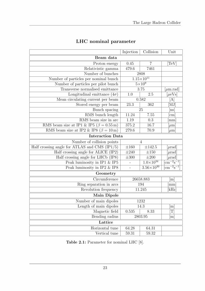
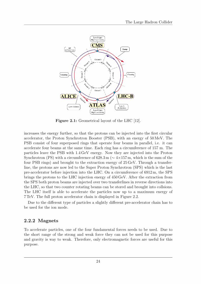
As the name implies, in the Large Hadron Collider two hadron beams are accelerated intwo separated rings and brought into collision at four interaction points (IP). Throughslightly different pre-accelerator chains, protons are accelerated up to a maximumenergy of 7 TeV per particle or, alternatively, lead ions up to 575 TeV per nucleus.Under nominal conditions one proton beam is made of 2808 bunches, each containsabout 1.15×10¹¹ particles, this means that the overall stored energy in one beam reachesaround 360 MJ, which is comparable to the energy of an aircraft carrier at half speed.The LHC will provide its four experiments ATLAS, ALICE, CMS and LHCb (seeFigure 2.1) with a luminosity of 1034 cm−2s−1. To force the particles on their circa26.7 km long circular obit, over 8000 superconducting magnets are used. From whichthe main dipole magnets reach a maximum strength of 8.3 T at top energy [8].
Apart from the magnets various other elements are required to obtain a stable andsecure operation with storage times of 10 hours and more. Some of them are introducedbriefly in the following section.
2.2.1 Injection System
Due to technical reasons it is not possible to inject the particles with a kinetic energyof nearly zero directly form the source into the LHC and accelerate them up to 7 TeV.There is no magnet that can cover a dynamic rage from 0 to 7 TeV. On the otherhand, it is difficult to reproduce very small magnetic fields, which would be neededat small kinetic energies, due to the remanence of the iron magnets. Hence, a chainof miscellaneous pre-accelerators is used to increase the energy step by step up to450 GeV, the injection energy of the LHC.
The pre-accelerator chain starts with a source of protons with a kinetic energy of90 keV from a duoplasmatron. It is followed by a radiofrequency quadrupole (RQF)which accelerates the particles up to 750 keV. The connected linear accelerator (LINAC2)
22
The Large Hadron Collider
LHC nominal parameter
Injection Collision Unit
Beam data
Proton energy 0.45 7 [TeV]Relativistic gamma 479.6 7461Number of bunches 2808
Number of particles per nominal bunch 1.15×10¹¹
Number of particles per pilot bunch 5×10⁹
Transverse normalised emittance 3.75 [µm.rad]Longitudinal emittance (4σ) 1.0 2.5 [µeVs]
Mean circulating current per beam 0.582 [A]Stored energy per beam 23.3 362 [MJ]
Bunch spacing 25 [ns]RMS bunch length 11.24 7.55 [cm]
RMS beam size in arc 1.19 0.3 [mm]RMS beam size at IP1 & IP5 (β = 0.55 m) 375.2 16.7 [µm]
RMS beam size at IP2 & IP8 (β = 10 m) 279.6 70.9 [µm]
Interaction Data
Number of collision points 4Half crossing angle for ATLAS and CMS (IP1/5) ±160 ±142.5 [µrad]
Half crossing angle for ALICE (IP2) ±240 ±150 [µrad]Half crossing angle for LHCb (IP8) ±300 ±200 [µrad]
Peak luminosity in IP1 & IP5 - 1.0×1034 [cm−2s−1]Peak luminosity in IP2 & IP8 - 3.56×1030 [cm−2s−1]
Geometry
Circumference 26658.883 [m]Ring separation in arcs 194 [mm]
Revolution frequency 11.245 [kHz]
Main Dipole
Number of main dipoles 1232Length of main dipoles 14.3 [m]
Magnetic field 0.535 8.33 [T]Bending radius 2803.95 [m]
Lattice
Horizontal tune 64.28 64.31Vertical tune 59.31 59.32
Table 2.1: Parameter for nominal LHC [8].
23
The Large Hadron Collider
Figure 2.1: Geometrical layout of the LHC [12].
increases the energy further, so that the protons can be injected into the first circularaccelerator, the Proton Synchrotron Booster (PSB), with an energy of 50 MeV. ThePSB consist of four superposed rings that operate four beams in parallel, i.e. it canaccelerate four beams at the same time. Each ring has a circumference of 157 m. Theparticles leave the PSB with 1.4 GeV energy. Now they are injected into the ProtonSynchrotron (PS) with a circumference of 628.3 m (∼ 4×157 m, which is the sum of thefour PSB rings) and brought to the extraction energy of 25 GeV. Through a transfer-line, the protons are now led to the Super Proton Synchrotron (SPS) which is the lastpre-accelerator before injection into the LHC. On a circumference of 6912 m, the SPSbrings the protons to the LHC injection energy of 450 GeV. After the extraction fromthe SPS both proton beams are injected over two transferlines in reverse directions intothe LHC, so that two counter rotating beams can be stored and brought into collsions.The LHC itself is able to accelerate the particles now up to a maximum energy of7 TeV. The full proton accelerator chain is displayed in Figure 2.2.
Due to the different type of particles a slightly different pre-accelerator chain has tobe used for the ion mode.
2.2.2 Magnets
To accelerate particles, one of the four fundamental forces needs to be used. Due tothe short range of the strong and weak force they can not be used for this purposeand gravity is way to weak. Therefore, only electromagnetic forces are useful for thispurpose.
24

The Large Hadron Collider
Figure 2.2: CERN accelerator complex to (pre-)accelerate the protons up to theirmaximum energy of 7 TeV [12].
On a particle with charge q and velocity ~v moving through the space in which amagnetic field ~B and an electric field ~E is present the Lorentz force
~F = q(~v × ~B + ~E) (2.1)
is exerted. The energy transferred to the particle is the integral over the covereddistance:
∆E = q∫ r2r1
(~v × ~B + ~E)d~r (2.2)
= q∫ r2r1~Ed~r = qU (2.3)
Since the velocity vector ~v is parallel to the direction vector ~r the scalar product(~v × ~B)d~r is zero. From this it can be concluded that only the electric field is respon-sible for the increase in energy of a charged particle, magnetic fields are only used fordeflection.
If a particle is deflected in a magnetic field, Lorentz and Centripetal force are alwaysequal. This leads to the beam rigidity Bρ:
FL = FC ⇐⇒mv2
ρ= qvB ⇐⇒ Bρ =
mv
q=p
q(2.4)
where ρ is the bending radius and p = mv the particle momentum. A multipole
25
The Large Hadron Collider
expansion of the magnetic field ~B and multiplication by e/p gives [13]
e
pBz(x) = e
pBz0 + e
pdBz
dxx+ 1
2!epd2Bz
dx2x2 + 1
3!epd3Bz
dx3x3 + ... (2.5)
= 1ρ
+ kx+ 12!mx2 + 1
3!ox3 + ... (2.6)
where the first term corresponds to a dipole, the second one to a quadrupole, the thirdone to a sextupole, the forth one to an octupole, etc. The magnetic field may thereforebe regarded as a sum of multipoles, each of which have a different effect on the pathof the particle. This can be used for different corrections on the beam.
Dipoles are used to bend the particles to a circular orbit to make them pass the samemachine elements over and over again.
Quadrupoles are used for the focusing. A particle accelerator is build in a way thatan ideal reference particle (i.e. a particle with design energy/momentum, ∆p
p= 0,
x = y = 0, x′ = y′ = 0) follows the design orbit, which lies in the middle of all machineelements. In absence of field errors and magnet misalignments focussing would not beneeded for such a design particle. But since the LHC operates under nominal conditionswith 2808 bunches each with 1.15×10¹¹ particles, it is unavoidable that some particleshave a slightly different momentum, an offset (x- or y-position) and/or an angle (x′ ory′) to the design orbit. Due to this variations the magnets apply a wrong deflectionon the particles which would lead to particle losses without the correction due to thefocussing effect of the quadrupoles.
By construction a horizontal focusing quadrupole is defocusing in the vertical plane,therefore one needs to locate a second quadrupole rotated by 90° some distance be-hind the first one to correct for this behaviour, a so-called FoDo-Cell is built. Thisalternating focusing-defocusing structure has to be repeated around the whole ring toforce the particles on a trajectory around the design orbit. More precisely, the particlesare excited to oscillate around the design orbit, the so-called betatron oscillation. Thenumber of oscillations a particle performs during one turn around the machine is calledtune. Every accelerator has two tune values, namely Qx in the horizontal and Qy inthe vertical plane. In general these two values are different. Only the fractional partcontains useful information for daily operation, since it can be varied by adjusting thestrength of the quadrupoles, whereas it is very unlikely that the number of completeoscillations will be changed. In daily operation when talking about the tune one alwaysrefers to the fractional part.
Nevertheless, certain fractional values of the tunes have to be avoided as they leadto resonant excitation and possible loss of the beam. If the condition
nQx +mQy = l (2.7)
is fulfilled, with n, m and l integers, the tune catches a resonance of order |n|+ |m|.In general, due to the finite mechanical tolerance and the limited pole width of the
magnets, all possible multipole fields are present in an accelerator. Hence, higher order
26
The Large Hadron Collider
Magnet Description
mainmagnets
MB dipole: main bending magnetMQ quadrupole: main focusing/defocusing magnet
dipolespoolpieces
MCS sextupole: corrects sextupolar component of the dipole fieldMCD decapole: corrects decapolar component of the dipole fieldMCO octupole: corrects octupolar component of the dipole field
correctorsattached to
mainquadrupoles
MCB dipole: corrects closed orbitMQT quadrupole: corrects tuneMQS skew quadrupole: rotated by 45°, corrects couplingMSC sextupole: corrects beam chromaticityMO octupole: Landau damping (damps beam excitations)
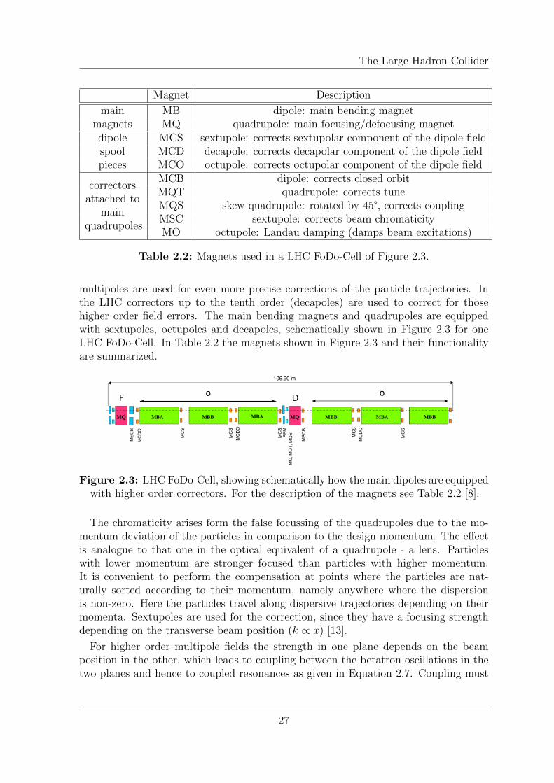
Table 2.2: Magnets used in a LHC FoDo-Cell of Figure 2.3.
multipoles are used for even more precise corrections of the particle trajectories. Inthe LHC correctors up to the tenth order (decapoles) are used to correct for thosehigher order field errors. The main bending magnets and quadrupoles are equippedwith sextupoles, octupoles and decapoles, schematically shown in Figure 2.3 for oneLHC FoDo-Cell. In Table 2.2 the magnets shown in Figure 2.3 and their functionalityare summarized.
Figure 2.3: LHC FoDo-Cell, showing schematically how the main dipoles are equippedwith higher order correctors. For the description of the magnets see Table 2.2 [8].
The chromaticity arises form the false focussing of the quadrupoles due to the mo-mentum deviation of the particles in comparison to the design momentum. The effectis analogue to that one in the optical equivalent of a quadrupole - a lens. Particleswith lower momentum are stronger focused than particles with higher momentum.It is convenient to perform the compensation at points where the particles are nat-urally sorted according to their momentum, namely anywhere where the dispersionis non-zero. Here the particles travel along dispersive trajectories depending on theirmomenta. Sextupoles are used for the correction, since they have a focusing strengthdepending on the transverse beam position (k ∝ x) [13].
For higher order multipole fields the strength in one plane depends on the beamposition in the other, which leads to coupling between the betatron oscillations in thetwo planes and hence to coupled resonances as given in Equation 2.7. Coupling must
27
The Large Hadron Collider
be avoided, since it is much easier to correct the two planes separately, rather than totake care of the second plane while applying corrections to the first one.
2.2.3 Closed Orbit Correctors
The Closed Orbit Dipoles (COD) are dipole magnets used to correct the closed orbit atLHC. They are individually powered magnets. Each dipole pair consists of a horizontal(vertical dipole field) and a vertical (horizontal dipole field) orbit corrector to applycorrections in both planes separately. The vertical corrector is realised by rotating thehorizontal one by 90°.
Taken beam 1 as reference, every horizontal COD is placed at the every focussingmain quadrupole. Correspondingly, every vertical COD is placed at every defocussingmain quadrupole. Therefore, the horizontal (vertical) correctors are separated by al-most 90° phase advance. The reason for this placement can be understood by consid-ering the equation of the closed orbit distortion (x) when a single dipole kick (x′) isperformed:
x(s) = x′(s0)
√β(s0)β(s)
2 sin(πQ)cos(|φ(s)− φ(s0)| − πQ) (2.8)
This equation depends on the β-function at the location of the kick, β(s0). The β-function has a maximum at the focussing quadrupoles, hence the effect of the kick isenhanced at this position and, consequently, the strenght of the dipoles can be relax.The dipole correctors in LHC work at a maximum current of 60 A.
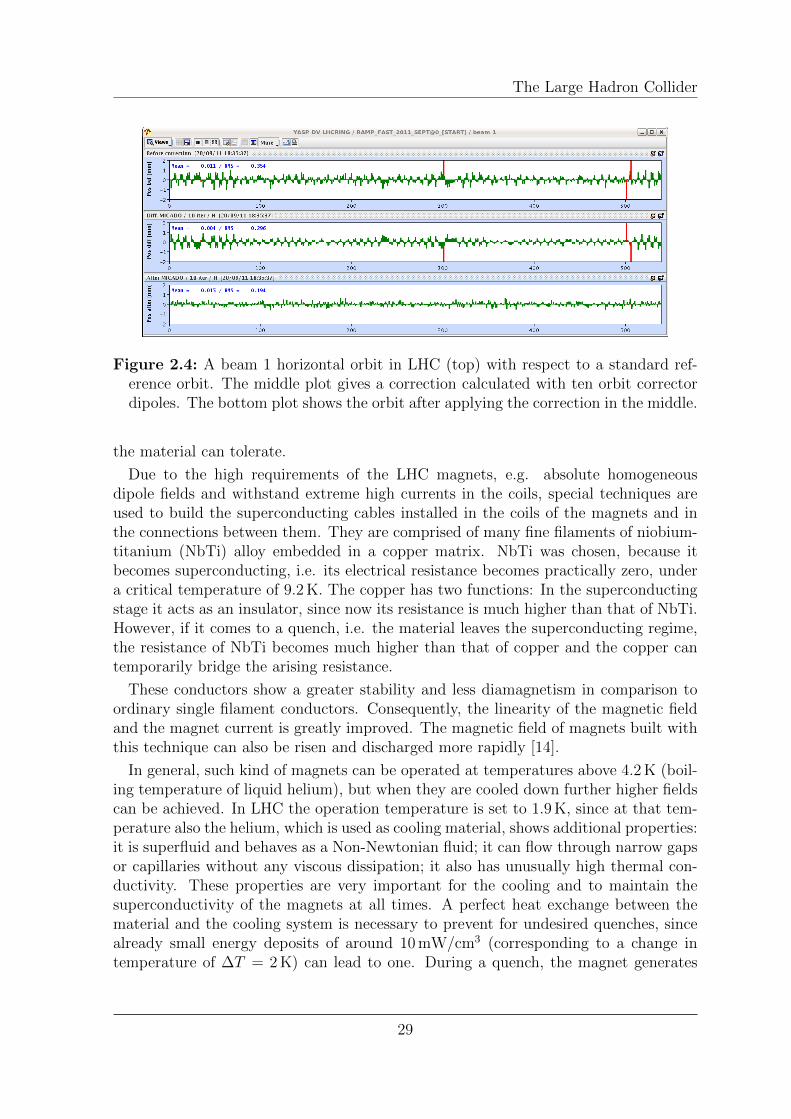
Figure 2.4 shows a difference orbit (top) of beam 1 with respect to a reference, as itis monitored in the control room. It was measured by the beam position monitors (seeChapter 2.3.2) directly after the injection of a pilot bunch. The used reference orbit isoptimized for the current collimator settings in the machine and can be loaded fromthe database. The middle plot indicates a possible correction to achieve the reference,calculated with ten corrector magnet. The bottom plot displays how the orbit wouldlook like after this correction is applied. The correction algorithm tries to obtain thereference orbit, therefore the bottom plot should be a zero orbit for a perfect correction.
2.2.4 Cryogenics and Superconductivity
Under nominal conditions the LHC stores protons with an energy of 7 TeV. By consid-ering Equation 2.4 again, one can easily determine that the strength of the magneticfield necessary to keep this protons on a circular orbit with a bending radius of around2800 m is B ≈ 8.3 T. With normal conducting magnets only a maximum field strengthof around 2 T can be reached. It poses a great challenge to techniques and materialto reach such high field strengths. Superconducting magnets are required, since themagnetic field strength B is proportional to the current I in the coils. Hence, theenergy is limited by the magnetic field strength or rather by the intensity of current
28
The Large Hadron Collider
Figure 2.4: A beam 1 horizontal orbit in LHC (top) with respect to a standard ref-erence orbit. The middle plot gives a correction calculated with ten orbit correctordipoles. The bottom plot shows the orbit after applying the correction in the middle.
the material can tolerate.
Due to the high requirements of the LHC magnets, e.g. absolute homogeneousdipole fields and withstand extreme high currents in the coils, special techniques areused to build the superconducting cables installed in the coils of the magnets and inthe connections between them. They are comprised of many fine filaments of niobium-titanium (NbTi) alloy embedded in a copper matrix. NbTi was chosen, because itbecomes superconducting, i.e. its electrical resistance becomes practically zero, undera critical temperature of 9.2 K. The copper has two functions: In the superconductingstage it acts as an insulator, since now its resistance is much higher than that of NbTi.However, if it comes to a quench, i.e. the material leaves the superconducting regime,the resistance of NbTi becomes much higher than that of copper and the copper cantemporarily bridge the arising resistance.
These conductors show a greater stability and less diamagnetism in comparison toordinary single filament conductors. Consequently, the linearity of the magnetic fieldand the magnet current is greatly improved. The magnetic field of magnets built withthis technique can also be risen and discharged more rapidly [14].
In general, such kind of magnets can be operated at temperatures above 4.2 K (boil-ing temperature of liquid helium), but when they are cooled down further higher fieldscan be achieved. In LHC the operation temperature is set to 1.9 K, since at that tem-perature also the helium, which is used as cooling material, shows additional properties:it is superfluid and behaves as a Non-Newtonian fluid; it can flow through narrow gapsor capillaries without any viscous dissipation; it also has unusually high thermal con-ductivity. These properties are very important for the cooling and to maintain thesuperconductivity of the magnets at all times. A perfect heat exchange between thematerial and the cooling system is necessary to prevent for undesired quenches, sincealready small energy deposits of around 10 mW/cm3 (corresponding to a change intemperature of ∆T = 2 K) can lead to one. During a quench, the magnet generates
29
The Large Hadron Collider
high internal voltages and locally elevated temperatures. These cause electrical andmechanical stresses in the windings. Permanent damage to the magnet can occur.
2.2.5 Radio Frequency Cavities
To accelerate the particles superconducting high frequency cavities are used. Per beamtwo times four cavities are installed in interaction region 4, see Figure 2.1. A maximalvoltage per beam of 8 MV at 450 GeV and of 16 MV at 7 TeV is reached at the RF-frequency of 400 MHz [8]. To maintain an optimal phase focussing this strength is notfully exploited. The energy gain per turn is only 485 keV, since the working point ofthe cavities is not set to the maximum amplitude of the high-frequency, rather to thetrailing edge. In that way high momentum particles gain less energy, because theyshow a slightly larger orbit radius with respect to the design particle and hence theyarrive later at the accelerating cavity. For low momentum particles it happens exactlythe other way around. Thus a longitudinal focussing is ensured.
2.2.6 Collimator System
Over the entire length of the accelerator 54 collimators per beam are installed whichbuild a passive security system. The collimators are used to absorb particles whichare deflected from the reference orbit and thus protect the beam pipe and the magnetsfrom unwanted impacts of these particles. If those particles would be absorbed by themagnets they could trigger a quench. Two main interaction points are used to rejectparticles with too large momentum (IP3) and amplitude deviation (IP7). Further col-limators are installed in front of the experiments and at the ends of the transfer lines.They are made of special plates consisting of graphite and tungsten. The most im-portant factor in the choice of the material was that the collimators have to be veryheat resistant, since they are meant to accumulate mislead particles to protect theother machine elements. The assembly is made of two shoes, each 1.6 m long, in thevacuum chamber which can be synchronously moved closer to the beam. In that wayit is possible to absorb 99.9 % of the dangerous particles before they are able to hit thewalls and magnets [8].
2.2.7 Beam Dump
After about 10 hours of stable beams the luminosity has decreased so much that thebeams need to be renewed. Therefore, a controlled dumping of the beams into theso-called beam dump must be triggered. The beams are deflected out of the beampipe by extraction kickers in point 6 (Figure 2.1) and lead to a 750 m long drift sectionwhich ends in a 7 m long and 70×70 cm width, water cooled and steel coated graphitebloc. This bloc is additionally surrounded by ∼ 900 t of radiation shielding blocs. Atthe moment the proton beam arrives at this structure its kinetic energy is transformedinto heat energy while a temperature of 800°C is reached [8].
30
The Large Hadron Collider
2.3 Measurement Devices for Beam Dynamics
A save and stable operation of such a huge accelerator implies that the beams arealways under control. During a run several beam parameters, like intensity, transverseposition, tune and beam size, are under constant review to be able to monitor thebeam behaviour and to apply corrections, if necessary. This is important for theoptimisation and safety of the machine but also to provide the experiments with thehighest luminosity possible.
To obtain the necessary information from the beam, several different devices forbeam diagnostics and instrumentation are needed. Due to the complexity of the LHCnot all instruments can be discussed in the scope of this thesis, but the ones used tocollect the data analysed here will be examined in the following.
2.3.1 Fast Beam Current Transformer (FBCT)
The beam current is one of the most important quantities for the operation of a par-ticle accelerator. It is one of the first parameter to be checked for the acceleratorfunctionality and to prevent for particle losses.
Many different devices can be used for this purpose, but for a continuous measure-ment of the beam current during operation a non-destructive device is needed. TheLHC uses a measurement method based on the detection of the magnetic field carriedby the beam, a so-called current transformer.
The Fast Beam Current Transformers (FBCTs) are capable of performing bunch-by-bunch measurements by integrating the charge of each LHC bunch. But they can alsoprovide information about the total turn-by-turn beam intensity. For redundancy, twofast transformers with totally separated acquisition chains are placed in each ring lo-cated in IR4. Moreover, each beam dump line is equipped with two redundant FBCTs,using the same acquisition electronics, for monitoring the ejected beams.
The beam consist of N particles with charge qe; these particles travel around thering, thus they can be regarded as a current
Ibeam =qeN
t(2.9)
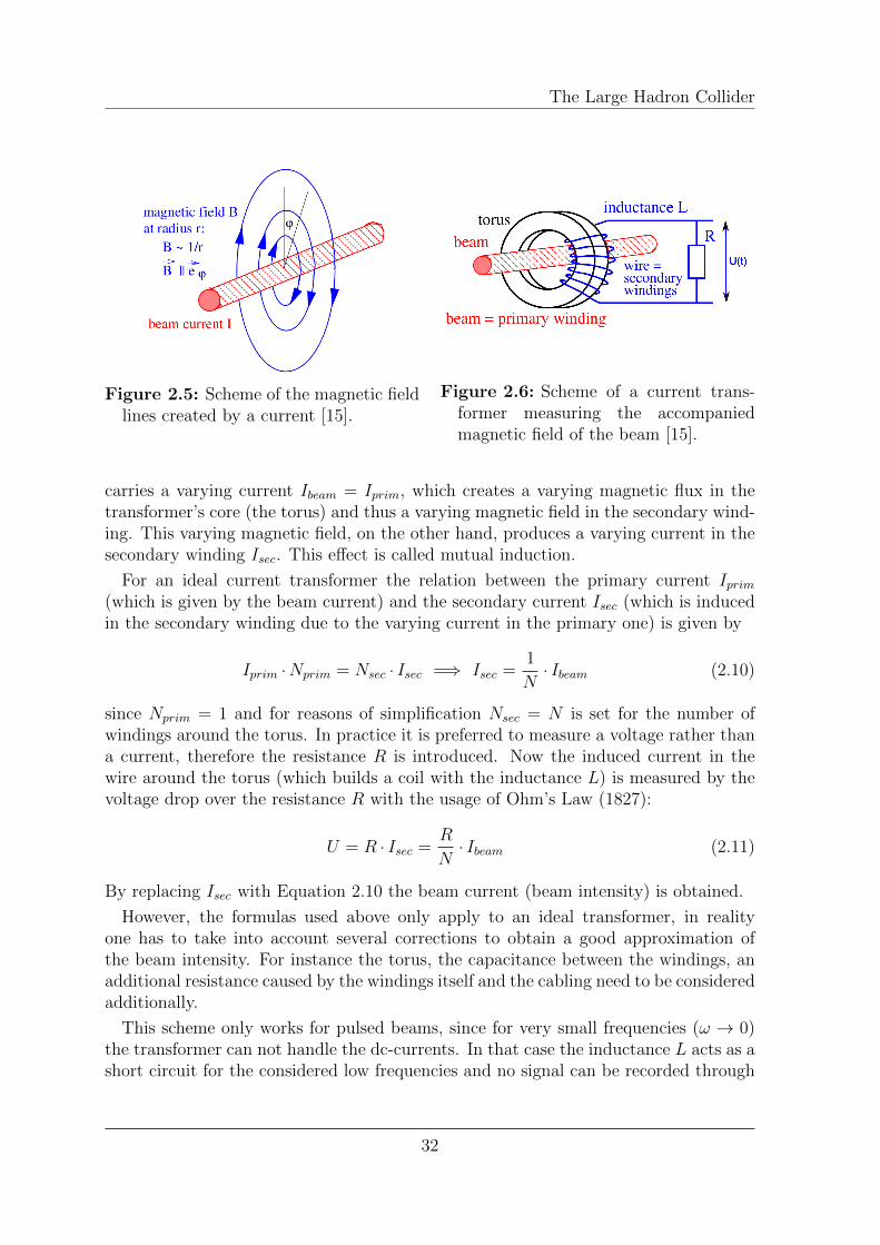
Like a current-carrying wire, the beam produces a magnetic field B as displayed inFigure 2.5 which can be calculated according to the Bio-Savart law (1820). Due to thecylindrical symmetry of the beam, only the azimuthal component has to be considered.Now the beam current can be determined by monitoring this accompanied magneticfield with a current transformer shown in Figure 2.6.
The beam passes as the ”primary winding” (Nprim = 1) of the transformer througha highly permeable torus. An insulated wire wound around the torus is acting asthe ”secondary winding” (Nsec). For a bunched beam it appears as this first winding
31
The Large Hadron Collider
Figure 2.5: Scheme of the magnetic fieldlines created by a current [15].
Figure 2.6: Scheme of a current trans-former measuring the accompaniedmagnetic field of the beam [15].
carries a varying current Ibeam = Iprim, which creates a varying magnetic flux in thetransformer’s core (the torus) and thus a varying magnetic field in the secondary wind-ing. This varying magnetic field, on the other hand, produces a varying current in thesecondary winding Isec. This effect is called mutual induction.
For an ideal current transformer the relation between the primary current Iprim(which is given by the beam current) and the secondary current Isec (which is inducedin the secondary winding due to the varying current in the primary one) is given by
Iprim ·Nprim = Nsec · Isec =⇒ Isec =1
N· Ibeam (2.10)
since Nprim = 1 and for reasons of simplification Nsec = N is set for the number ofwindings around the torus. In practice it is preferred to measure a voltage rather thana current, therefore the resistance R is introduced. Now the induced current in thewire around the torus (which builds a coil with the inductance L) is measured by thevoltage drop over the resistance R with the usage of Ohm’s Law (1827):
U = R · Isec =R
N· Ibeam (2.11)
By replacing Isec with Equation 2.10 the beam current (beam intensity) is obtained.
However, the formulas used above only apply to an ideal transformer, in realityone has to take into account several corrections to obtain a good approximation ofthe beam intensity. For instance the torus, the capacitance between the windings, anadditional resistance caused by the windings itself and the cabling need to be consideredadditionally.
This scheme only works for pulsed beams, since for very small frequencies (ω → 0)the transformer can not handle the dc-currents. In that case the inductance L acts as ashort circuit for the considered low frequencies and no signal can be recorded through
32
The Large Hadron Collider
the resistor [15].
However, with this technique very low currents and thus very low intensities can bemeasured. Furthermore, due to the fact that the torus only detects the azimuthal fieldcomponent the signal is nearly independent of the displacement of the beam from thecentral orbit.
2.3.2 Beam Position Monitor (BPM)
A Beam Position Monitor (BPM) is a non-destructive diagnostic instrument with whichthe position of the beam in the beam pipe can be measured. In the daily operationof an accelerator it is very important to know the position of the beam to check andcorrect for position offsets, since these lead to wrong deflections of the particles by themagnets.
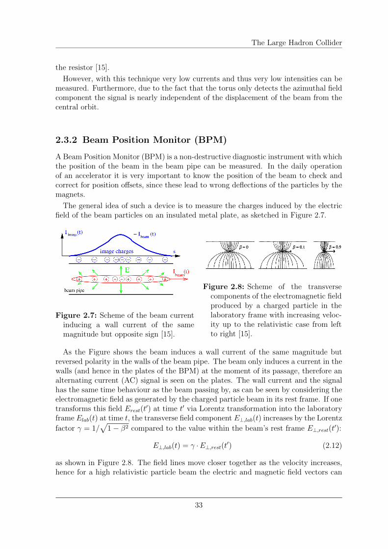
The general idea of such a device is to measure the charges induced by the electricfield of the beam particles on an insulated metal plate, as sketched in Figure 2.7.
Figure 2.7: Scheme of the beam currentinducing a wall current of the samemagnitude but opposite sign [15].
Figure 2.8: Scheme of the transversecomponents of the electromagnetic fieldproduced by a charged particle in thelaboratory frame with increasing veloc-ity up to the relativistic case from leftto right [15].
As the Figure shows the beam induces a wall current of the same magnitude butreversed polarity in the walls of the beam pipe. The beam only induces a current in thewalls (and hence in the plates of the BPM) at the moment of its passage, therefore analternating current (AC) signal is seen on the plates. The wall current and the signalhas the same time behaviour as the beam passing by, as can be seen by considering theelectromagnetic field as generated by the charged particle beam in its rest frame. If onetransforms this field Erest(t
′) at time t′ via Lorentz transformation into the laboratoryframe Elab(t) at time t, the transverse field component E⊥,lab(t) increases by the Lorentz
factor γ = 1/√
1− β2 compared to the value within the beam’s rest frame E⊥,rest(t′):
E⊥,lab(t) = γ ·E⊥,rest(t′) (2.12)
as shown in Figure 2.8. The field lines move closer together as the velocity increases,hence for a high relativistic particle beam the electric and magnetic field vectors can
33
The Large Hadron Collider
be approximated as perpendicular to the propagating direction. This is the behaviourof a so-called Transverse Electric and Magnetic (TEM) field distribution.
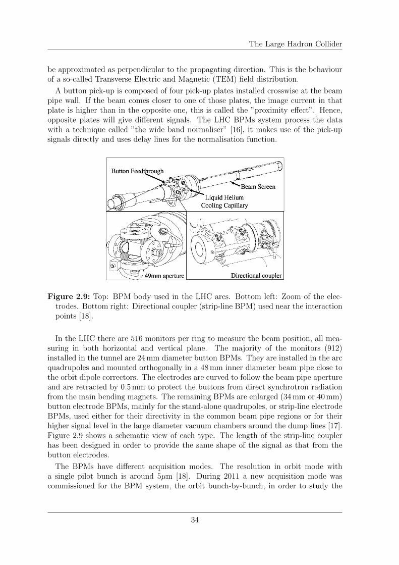
A button pick-up is composed of four pick-up plates installed crosswise at the beampipe wall. If the beam comes closer to one of those plates, the image current in thatplate is higher than in the opposite one, this is called the ”proximity effect”. Hence,opposite plates will give different signals. The LHC BPMs system process the datawith a technique called ”the wide band normaliser” [16], it makes use of the pick-upsignals directly and uses delay lines for the normalisation function.
Figure 2.9: Top: BPM body used in the LHC arcs. Bottom left: Zoom of the elec-trodes. Bottom right: Directional coupler (strip-line BPM) used near the interactionpoints [18].
In the LHC there are 516 monitors per ring to measure the beam position, all mea-suring in both horizontal and vertical plane. The majority of the monitors (912)installed in the tunnel are 24 mm diameter button BPMs. They are installed in the arcquadrupoles and mounted orthogonally in a 48 mm inner diameter beam pipe close tothe orbit dipole correctors. The electrodes are curved to follow the beam pipe apertureand are retracted by 0.5 mm to protect the buttons from direct synchrotron radiationfrom the main bending magnets. The remaining BPMs are enlarged (34 mm or 40 mm)button electrode BPMs, mainly for the stand-alone quadrupoles, or strip-line electrodeBPMs, used either for their directivity in the common beam pipe regions or for theirhigher signal level in the large diameter vacuum chambers around the dump lines [17].Figure 2.9 shows a schematic view of each type. The length of the strip-line couplerhas been designed in order to provide the same shape of the signal as that from thebutton electrodes.
The BPMs have different acquisition modes. The resolution in orbit mode witha single pilot bunch is around 5µm [18]. During 2011 a new acquisition mode wascommissioned for the BPM system, the orbit bunch-by-bunch, in order to study the
34
The Large Hadron Collider
beam-beam orbit effects. Results about the linearity and resolution of this mode aregiven in Section 4.2.2.
2.3.3 Wire Scanner
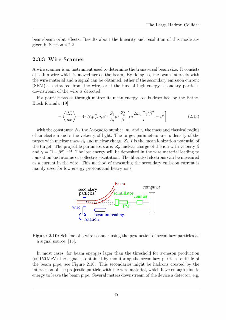
A wire scanner is an instrument used to determine the transversal beam size. It consistsof a thin wire which is moved across the beam. By doing so, the beam interacts withthe wire material and a signal can be obtained, either if the secondary emission current(SEM) is extracted from the wire, or if the flux of high-energy secondary particlesdownstream of the wire is detected.
If a particle passes through matter its mean energy loss is described by the Bethe-Bloch formula [19]
−⟨dE
dx
⟩= 4πNAr
2emec
2 ·ZtAtρ ·Z2p
β
[ln
2mec2γ2β2
I− β2
](2.13)
with the constants: NA the Avogadro number, me and re the mass and classical radiusof an electron and c the velocity of light. The target parameters are: ρ density of thetarget with nuclear mass At and nuclear charge Zt, I is the mean ionization potential ofthe target. The projectile parameters are: Zp nuclear charge of the ion with velocity βand γ = (1−β2)−1/2. The lost energy will be deposited in the wire material leading toionization and atomic or collective excitation. The liberated electrons can be measuredas a current in the wire. This method of measuring the secondary emission current ismainly used for low energy protons and heavy ions.
Figure 2.10: Scheme of a wire scanner using the production of secondary particles asa signal source, [15].
In most cases, for beam energies lager than the threshold for π-meson production(≈ 150 MeV) the signal is obtained by monitoring the secondary particles outside ofthe beam pipe, see Figure 2.10. This secondaries might be hadrons created by theinteraction of the projectile particle with the wire material, which have enough kineticenergy to leave the beam pipe. Several meters downstream of the device a detector, e.g.
35
The Large Hadron Collider
Figure 2.11: Left: Foto of a wire scanner used at CERN [15]. Right: Scheme of thewire scanner position inside the beam pipe [20].
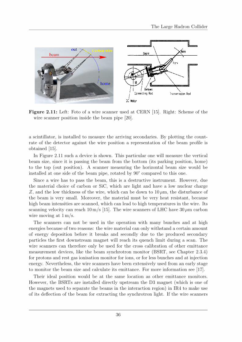
a scintillator, is installed to measure the arriving secondaries. By plotting the count-rate of the detector against the wire position a representation of the beam profile isobtained [15].
In Figure 2.11 such a device is shown. This particular one will measure the verticalbeam size, since it is passing the beam from the bottom (its parking position, home)to the top (out position). A scanner measuring the horizontal beam size would beinstalled at one side of the beam pipe, rotated by 90° compared to this one.
Since a wire has to pass the beam, this is a destructive instrument. However, duethe material choice of carbon or SiC, which are light and have a low nuclear chargeZ, and the low thickness of the wire, which can be down to 10µm, the disturbance ofthe beam is very small. Moreover, the material must be very heat resistant, becausehigh beam intensities are scanned, which can lead to high temperatures in the wire. Itsscanning velocity can reach 10 m/s [15]. The wire scanners of LHC have 30µm carbonwire moving at 1 m/s.
The scanners can not be used in the operation with many bunches and at highenergies because of two reasons: the wire material can only withstand a certain amountof energy deposition before it breaks and secondly due to the produced secondaryparticles the first downstream magnet will reach its quench limit during a scan. Thewire scanners can therefore only be used for the cross calibration of other emittancemeasurement devices, like the beam synchrotron monitor (BSRT, see Chapter 2.3.4)for protons and rest gas ionisation monitor for ions, or for less bunches and at injectionenergy. Nevertheless, the wire scanners have been extensively used from an early stageto monitor the beam size and calculate its emittance. For more information see [17].
Their ideal position would be at the same location as other emittance monitors.However, the BSRTs are installed directly upstream the D3 magnet (which is one ofthe magnets used to separate the beams in the interaction region) in IR4 to make useof its deflection of the beam for extracting the synchrotron light. If the wire scanners
36
The Large Hadron Collider
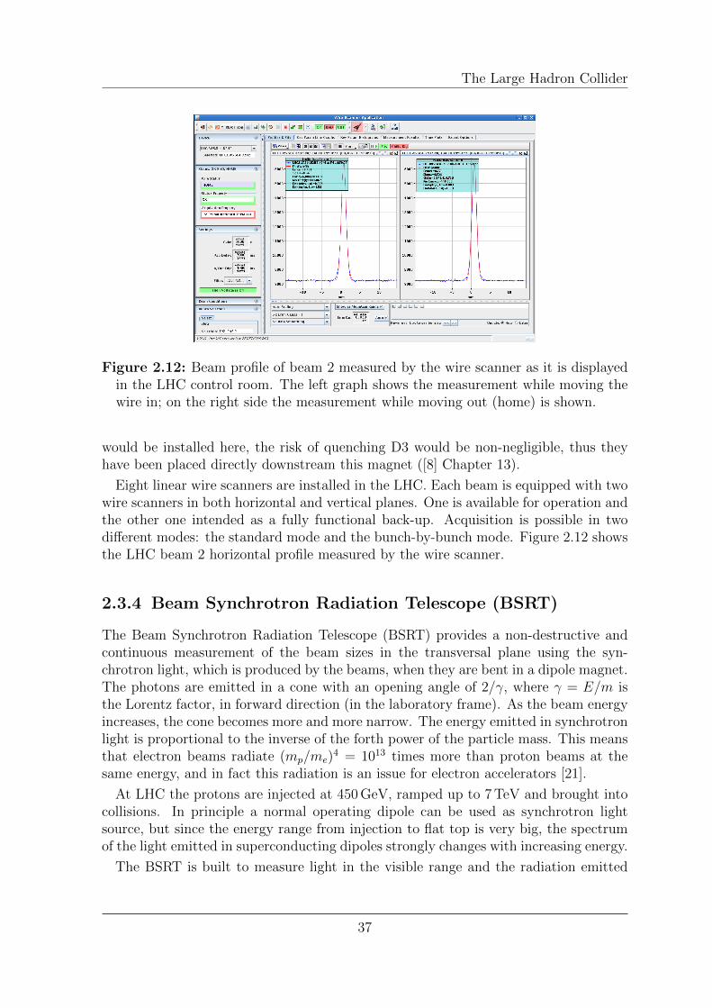
Figure 2.12: Beam profile of beam 2 measured by the wire scanner as it is displayedin the LHC control room. The left graph shows the measurement while moving thewire in; on the right side the measurement while moving out (home) is shown.
would be installed here, the risk of quenching D3 would be non-negligible, thus theyhave been placed directly downstream this magnet ([8] Chapter 13).
Eight linear wire scanners are installed in the LHC. Each beam is equipped with twowire scanners in both horizontal and vertical planes. One is available for operation andthe other one intended as a fully functional back-up. Acquisition is possible in twodifferent modes: the standard mode and the bunch-by-bunch mode. Figure 2.12 showsthe LHC beam 2 horizontal profile measured by the wire scanner.
2.3.4 Beam Synchrotron Radiation Telescope (BSRT)
The Beam Synchrotron Radiation Telescope (BSRT) provides a non-destructive andcontinuous measurement of the beam sizes in the transversal plane using the syn-chrotron light, which is produced by the beams, when they are bent in a dipole magnet.The photons are emitted in a cone with an opening angle of 2/γ, where γ = E/m isthe Lorentz factor, in forward direction (in the laboratory frame). As the beam energyincreases, the cone becomes more and more narrow. The energy emitted in synchrotronlight is proportional to the inverse of the forth power of the particle mass. This meansthat electron beams radiate (mp/me)
4 = 1013 times more than proton beams at thesame energy, and in fact this radiation is an issue for electron accelerators [21].
At LHC the protons are injected at 450 GeV, ramped up to 7 TeV and brought intocollisions. In principle a normal operating dipole can be used as synchrotron lightsource, but since the energy range from injection to flat top is very big, the spectrumof the light emitted in superconducting dipoles strongly changes with increasing energy.
The BSRT is built to measure light in the visible range and the radiation emitted
37
The Large Hadron Collider
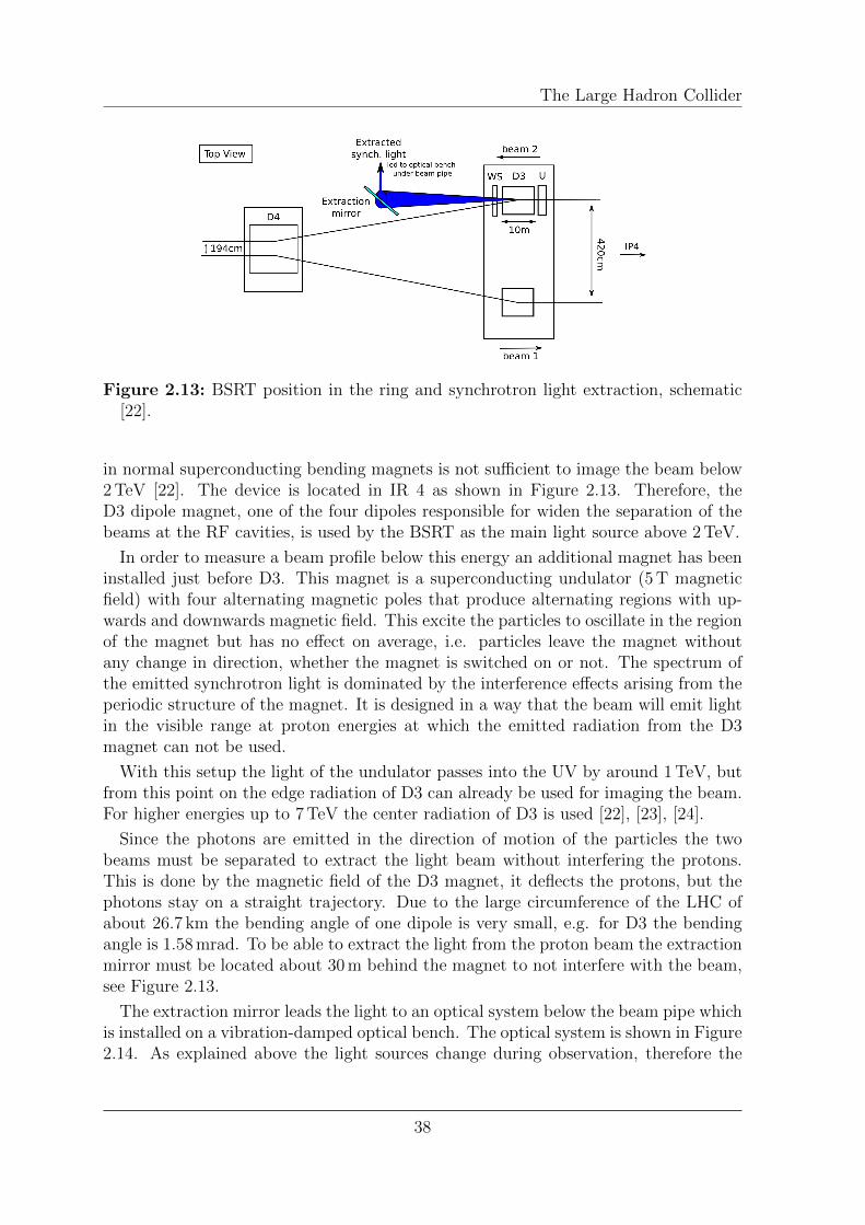
Figure 2.13: BSRT position in the ring and synchrotron light extraction, schematic[22].
in normal superconducting bending magnets is not sufficient to image the beam below2 TeV [22]. The device is located in IR 4 as shown in Figure 2.13. Therefore, theD3 dipole magnet, one of the four dipoles responsible for widen the separation of thebeams at the RF cavities, is used by the BSRT as the main light source above 2 TeV.
In order to measure a beam profile below this energy an additional magnet has beeninstalled just before D3. This magnet is a superconducting undulator (5 T magneticfield) with four alternating magnetic poles that produce alternating regions with up-wards and downwards magnetic field. This excite the particles to oscillate in the regionof the magnet but has no effect on average, i.e. particles leave the magnet withoutany change in direction, whether the magnet is switched on or not. The spectrum ofthe emitted synchrotron light is dominated by the interference effects arising from theperiodic structure of the magnet. It is designed in a way that the beam will emit lightin the visible range at proton energies at which the emitted radiation from the D3magnet can not be used.
With this setup the light of the undulator passes into the UV by around 1 TeV, butfrom this point on the edge radiation of D3 can already be used for imaging the beam.For higher energies up to 7 TeV the center radiation of D3 is used [22], [23], [24].
Since the photons are emitted in the direction of motion of the particles the twobeams must be separated to extract the light beam without interfering the protons.This is done by the magnetic field of the D3 magnet, it deflects the protons, but thephotons stay on a straight trajectory. Due to the large circumference of the LHC ofabout 26.7 km the bending angle of one dipole is very small, e.g. for D3 the bendingangle is 1.58 mrad. To be able to extract the light from the proton beam the extractionmirror must be located about 30 m behind the magnet to not interfere with the beam,see Figure 2.13.
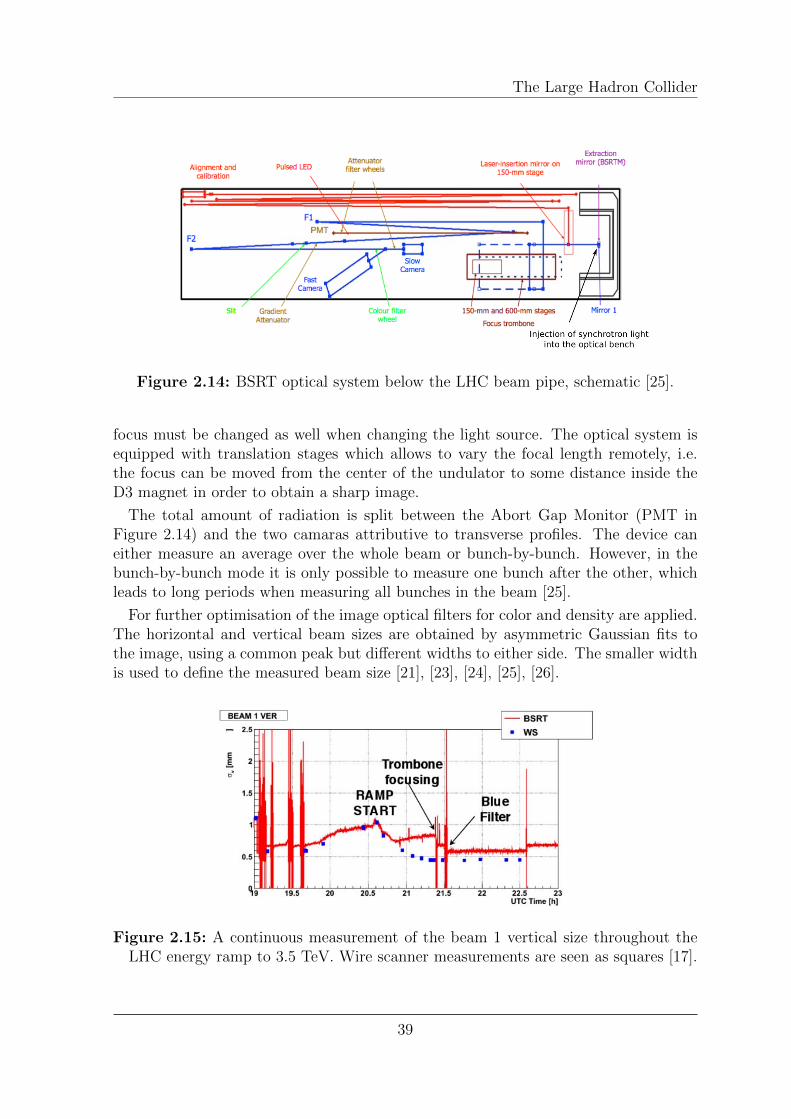
The extraction mirror leads the light to an optical system below the beam pipe whichis installed on a vibration-damped optical bench. The optical system is shown in Figure2.14. As explained above the light sources change during observation, therefore the
38
The Large Hadron Collider
Figure 2.14: BSRT optical system below the LHC beam pipe, schematic [25].
focus must be changed as well when changing the light source. The optical system isequipped with translation stages which allows to vary the focal length remotely, i.e.the focus can be moved from the center of the undulator to some distance inside theD3 magnet in order to obtain a sharp image.
The total amount of radiation is split between the Abort Gap Monitor (PMT inFigure 2.14) and the two camaras attributive to transverse profiles. The device caneither measure an average over the whole beam or bunch-by-bunch. However, in thebunch-by-bunch mode it is only possible to measure one bunch after the other, whichleads to long periods when measuring all bunches in the beam [25].
For further optimisation of the image optical filters for color and density are applied.The horizontal and vertical beam sizes are obtained by asymmetric Gaussian fits tothe image, using a common peak but different widths to either side. The smaller widthis used to define the measured beam size [21], [23], [24], [25], [26].
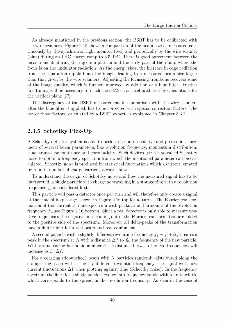
Figure 2.15: A continuous measurement of the beam 1 vertical size throughout theLHC energy ramp to 3.5 TeV. Wire scanner measurements are seen as squares [17].
39
The Large Hadron Collider
As already mentioned in the previous section, the BSRT has to be calibrated withthe wire scanners. Figure 2.15 shows a comparison of the beam size as measured con-tinuously by the synchrotron light monitor (red) and periodically by the wire scanner(blue) during an LHC energy ramp to 3.5 TeV. There is good agreement between themeasurements during the injection plateau and the early part of the ramp, where thefocus is on the undulator radiation. As the energy rises, the increase in edge radiationfrom the separation dipole blurs the image, leading to a measured beam size largerthan that given by the wire scanners. Adjusting the focussing trombone recovers someof the image quality, which is further improved by addition of a blue filter. Furtherfine tuning will be necessary to reach the 3-5% error level predicted by calculations forthe vertical plane [17].
The discrepancy of the BSRT measurement in comparison with the wire scannersafter the blue filter is applied, has to be corrected with special correction factors. Theuse of those factors, calculated by a BSRT expert, is explained in Chapter 3.3.2.
2.3.5 Schottky Pick-Up
A Schottky detector system is able to perform a non-destructive and precise measure-ment of several beam parameters, like revolution frequency, momentum distribution,tune, transverse emittance and chromaticity. Such devices use the so-called Schottkynoise to obtain a frequency spectrum from which the mentioned parameter can be cal-culated. Schottky noise is produced by statistical fluctuations which a current, createdby a finite number of charge carriers, always shows.
To understand the origin of Schottky noise and how the measured signal has to beinterpreted, a single particle with charge qe travelling in a storage ring with a revolutionfrequence f0 is considered first.
This particle will pass a detector once per turn and will therefore only create a signalat the time of its passage, shown in Figure 2.16 top for m turns. The Fourier transfor-mation of this current is a line spectrum with peaks at all harmonics of the revolutionfrequency f0, see Figure 2.16 bottom. Since a real detector is only able to measure pos-itive frequencies the negative ones coming out of the Fourier transformation are foldedto the positive side of the spectrum. Moreover, all delta-peaks of the transformationhave a finite hight for a real beam and real equipment.
A second particle with a slightly different revolution frequency f1 = f0+∆f creates apeak in the spectrum at f1 with a distance ∆f to f0, the frequency of the first particle.With an increasing harmonic number h the distance between the two frequencies willincrease as h · ∆f .
For a coasting (debunched) beam with N particles randomly distributed along thestorage ring, each with a slightly different revolution frequency, the signal will showcurrent fluctuations ∆I when plotting against time (Schottky noise). In the frequencyspectrum the lines for a single particle evolve into frequency bands with a finite width,which corresponds to the spread in the revolution frequency. As seen in the case of
40
The Large Hadron Collider
Figure 2.16: Single particle time do-main signal and line frequency spec-trum in a storage ring [15].
Figure 2.17: Sidebands (blue) appearingaround the center longitudinal Schottkysignal (red) due to transversal betatron os-cillation [15].
only two particles, the width of the bands increases with the harmonic number, butsince the total power within a band is constant, the hight must decreases.
Furthermore, the coasting beam also shows a transversal oscillation around the ref-erence orbit, the so-called betatron oscillation. With a position-sensitive pick-up one isable to obtain the transverse position from the difference signal of opposite electrodes,like it is done for a Beam Position Monitor (BPM). The output signal of such a pick-up has two contributions, one corresponds to the already seen longitudinal Schottkysignal, the other one appears as a frequency modulation of this signal caused by thetransversal betatron oscillation. It can be calculated that this will cause sidebandswith the maximum located at
∆f±h = (h± q) · f0 (2.14)
for a fixed harmonic number, see Figure 2.17. From this position the non-integer partof the tune q can be calculated via
q =f+h − f
−h
2f0
(2.15)
The appearance of two mirroring sidebands, again arise from the definition of thefrequency range of the Fourier transformation (−∞ to +∞), in a real detector onlypositive frequencies can be measured.
This gives an easy measurement of the incoherent value of the tune without influ-encing the beam. However, with this formalism one implies that the non-integer part
41

The Large Hadron Collider
of the tune is smaller than 0.5. But without any additional information one can nottell if q is above or below 0.5.
From the width of the sidebands the chromaticity can be determined. While thewidth is given by
∆f±h = ∆f0(h± q)±∆qf0 (2.16)
inserting the formula for the frequency dispersion η = 1γ2tr− 1
γ2(where α = 1
γ2tris
the momentum compaction factor) and the chromaticity ξ = ∆pp/∆QQ
(where p is the
momentum and Q is the tune of the particles), that leads to
∆f+h = η∆p
p· f0
(h+ q − ξ
ηQ)
upper sideband (2.17)
∆f−h = η∆pp
· f0
(h− q + ξ
ηQ)
lower sideband (2.18)
It can be seen, that the widths of the two sidebands are not equal. To obtain thechromaticity the other parameters ∆p
p, η and q has to be measured independently.
As mentioned above the width is also related to the frequency spread and thus tothe momentum spread. Equation 2.17 and 2.18 gives
∆p
p=
1
η
∆f+h + ∆f−h2hf0
(2.19)
When also the amplitude of the sidebands A are taken into account, the emittancecan be calculated via
ε ∝ A+h f
+h + A−h f
−h (2.20)
For bunched beams each bunch can oscillate longitudinally inside its bucket. Thismotion is called synchrotron oscillation and causes additional sidebands to each har-monic line h · f0 (center of the Schottky bands), since it modifies the time the particlesare passing through the detector. From the distance between the maxima the syn-chrotron frequency can be determined. If betatron motion is present, the betatronsidebands are modulated due to synchrotron oscillation as well. This causes a quitecomplex spectrum [15], [21].
In the LHC a 4.8 GHz slotted waveguide structure Schottky pick-up, schematicallyshown in Figure 2.18, is used. It has an aperture of 60×60 mm and is 1.5 m long.A gated, triple down-mixing scheme is used to baseband the successive filtering frombandwidth of 100 MHz to 11 kHz. This device is capable of bunch-by-bunch measure-ments [27]. Four pick-ups are installed near point 4 in a normal conducting straightsection, one per plane and beam. The transversal sensitivity is designed to peak at4.8 GHz, since this is a multiple integer number of the 40 MHz revolution frequency of
42

The Large Hadron Collider
the 25 ns bunch spacing under nominal conditions [28]. Figure 2.19 shows an exampleof a Schottky spectrum measured with the LHC monitors.
Figure 2.18: Scheme of the slotted waveguide structure for the LHC Schottky pick-up[28].
Figure 2.19: Schottky spectrum measured with the LHC Schottky pick-ups. Twosmall peaks directly to both sides of the revolution frequency peak (middle) are thesidebands used to determine the tune. Left: beam 1, right: beam 2, top: horizontal,bottom: vertical.
43
The Large Hadron Collider
2.3.6 Machine Luminosity Monitors (BRAN)
The aim of the machine luminosity monitors [29], namely Beam RAte of Neutrals(BRAN), is to measure the interaction rates for the setup, the optimization and theequalization of the beams at the interaction regions. These instruments are required tomeasure the interaction rate with a good relative accuracy; the absolute value can beobtained with frequent cross calibrations against the luminosity monitors installed inthe experiments. The calibration factor must remain stable over a reasonable amountof time and must not be influenced by the machine parameters (steering, optics etc.)The main error component from the BRAN detectors is expected to be the background.The requirements on the accuracy go from around 10% for the beam finding mode to0.25% for the luminosity optimization phase. The integration time per scan pointis inversely proportional to the luminosity for a given error. In order to detect andcorrect eventual bunch-by-bunch effects the bunch-by-bunch luminosity measurementis required. The detectors, readout and acquisition systems must thus be capable ofoperating with a useful bandwidth of 40 MHz.
The machine luminosity monitors are installed in the TAN absorbers 141 m awayon either side of IP1 and IP5; and 113 m away on either side of IP2 and IP8. Themonitors measure the flux of the showers generated by the neutral particles created inthe collisions (neutrons and photons). Neutral particles are chosen in order to suppressthe background related to beam losses. An schematic layout of the IP can be seen inFigure 2.20.
The radiation dose to the detectors is very large, 170 MGy/yr, and poses a con-straint on the choice of the technology. For the high luminosity experiments (ALTASand CMS) the monitors are radiation hard ionization chambers developed at LBNL(Lawrence Berkeley National Laboratory). The other interaction points have Cad-mium Telluride (CdTe) detectors which are CERN responsibility. The CdTe detectorscan easily comply with the 40 MHz bandwith, which is not the case for the ionizationchambers, but they can only stand the radiation doses foreseen at ALICE and LHCb[30].
Figure 2.20: Layout of a high luminosity IP in LHC with the BRAN detectors placedat the copper absorber called TAN (orange rectangle) [30].
44
Linear Coherent Beam-Beam Parameter
3 Linear Coherent Beam-BeamParameter
In a particle collider like the LHC it is desirable to have colliding beams to provide theexperiments with a high luminosity. But bringing the beams into collisions leads toadditional effects which influences the stability and lifetime of the beam. These beam-beam effects can be one of the most important limiting factors in a collider, thereforethey must be studied in detail.
However, a well defined limit like in lepton colliders [2] does not exist for hadronmachines like the LHC, but possible indications for a limiting head-on beam-beameffect may be [31]:
• Slow emittance increase
• Beam losses and bad lifetime
• Coherent beam-beam oscillations
To find the optimal strategy for the LHC luminosity upgrade it is important to know,if the limiting factors are the head-on or long-range interactions.
In this chapter the linear coherent beam-beam parameter is calculated from the dataof dedicated machine studies which took place during specific machine development(MD) periods.
This parameter is very useful as it is an estimation of the maximum linear coherenttune shift due to beam-beam interactions in the head-on case. It can give and approx-imation of the strength of the beam-beam interactions in single collisions and can besuperimposed to get an estimation if more collisions per turn are present. However,it does not reflect the non-linearity of the beam-beam force and can therefore only beused as a scaling parameter in the linear regime for beam separations smaller than onein terms of beam size σ, which only applies to the head-on case.
The most important effect head-on collisions introduce is a change in tune (seeChapter 1.2). In LHC, with two colliding proton beams, the tune shift is negative. Asa result the tune is decreased and moved in the tune diagram, with possible crossingof resonances, which can cause particle losses and lifetime problems. If the effect is toolarge, a tune scan must be performed to find a more optimal tune on which the beamsare stable again.
For the incoherent case this parameter is derived from the kick a beam exerts toa single particle in the opposite beam as shown in Chapter 1.2. However, in dailyoperation two bunches are colliding, those are an ensemble of about 1.1×10¹¹ particles.
45
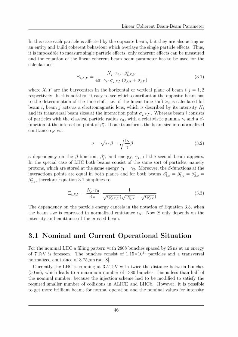
Linear Coherent Beam-Beam Parameter
In this case each particle is affected by the opposite beam, but they are also acting asan entity and build coherent behaviour which overlays the single particle effects. Thus,it is impossible to measure single particle effects, only coherent effects can be measuredand the equation of the linear coherent beam-beam parameter has to be used for thecalculations:
Ξi,X,Y =Nj · r0,i · β∗i,X,Y
4π · γi ·σj,X,Y (σj,X + σj,Y )(3.1)
where X, Y are the barycentres in the horizontal or vertical plane of beam i, j = 1, 2respectively. In this notation it easy to see which contribution the opposite beam hasto the determination of the tune shift, i.e. if the linear tune shift Ξi is calculated forbeam i, beam j acts as a electromagnetic lens, which is described by its intensity Nj
and its transversal beam sizes at the interaction point σj,X,Y . Whereas beam i consistsof particles with the classical particle radius r0,i with a relativistic gamma γi and a β-function at the interaction point of β∗i . If one transforms the beam size into normalizedemittance εN via
σ =√ε · β =
√εNγβ (3.2)
a dependency on the β-function, β∗j , and energy, γj, of the second beam appears.In the special case of LHC both beams consist of the same sort of particles, namelyprotons, which are stored at the same energy γ1 = γ2. Moreover, the β-functions at theinteractions points are equal in both planes and for both beams β∗1,x = β∗1,y = β∗2,x =β∗2,y, therefore Equation 3.1 simplifies to
Ξi,X,Y =Nj · r0
4π·
1√εNj,X,Y
(√εNj,X
+√εNj,Y
)(3.3)
The dependency on the particle energy cancels in the notation of Equation 3.3, whenthe beam size is expressed in normalized emittance εN . Now Ξ only depends on theintensity and emittance of the crossed beam.
3.1 Nominal and Current Operational Situation
For the nominal LHC a filling pattern with 2808 bunches spaced by 25 ns at an energyof 7 TeV is foreseen. The bunches consist of 1.15×10¹¹ particles and a transversalnormalized emittance of 3.75µm rad [8].
Currently the LHC is running at 3.5 TeV with twice the distance between bunches(50 ns), which leads to a maximum number of 1380 bunches, this is less than half ofthe nominal number, because the injection scheme had to be modified to satisfy therequired smaller number of collisions in ALICE and LHCb. However, it is possibleto get more brilliant beams for normal operation and the nominal values for intensity
46
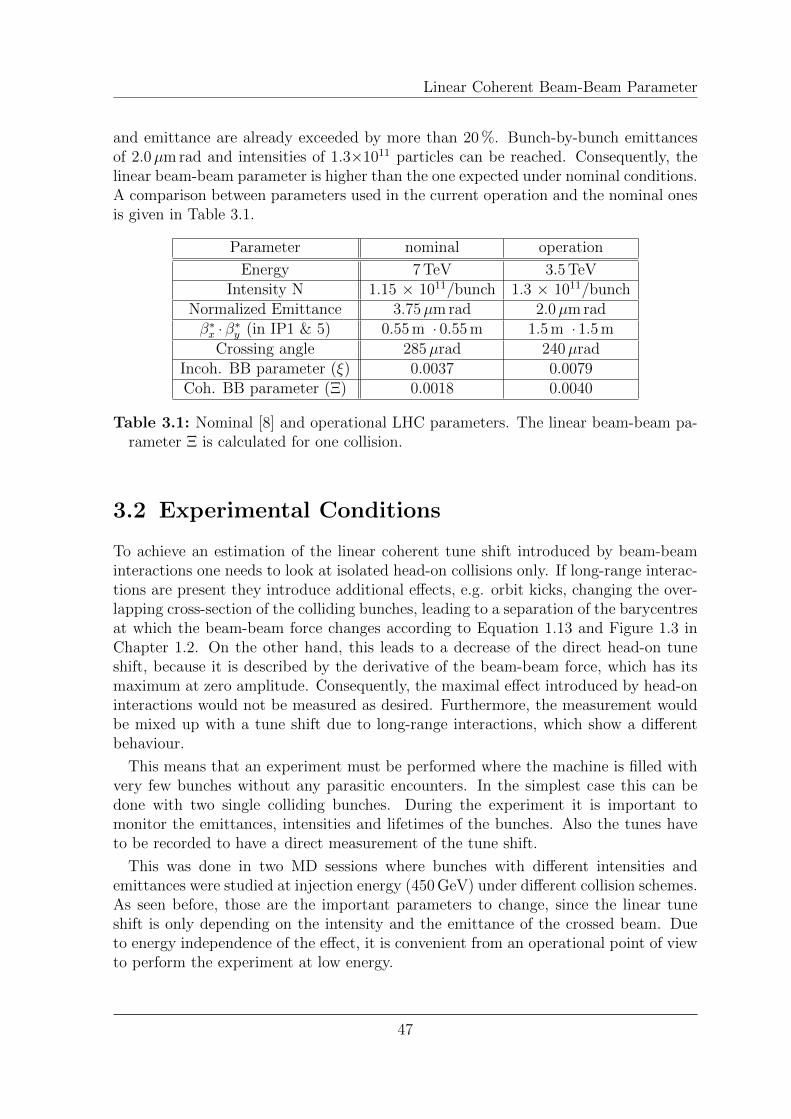
Linear Coherent Beam-Beam Parameter
and emittance are already exceeded by more than 20 %. Bunch-by-bunch emittancesof 2.0µm rad and intensities of 1.3×10¹¹ particles can be reached. Consequently, thelinear beam-beam parameter is higher than the one expected under nominal conditions.A comparison between parameters used in the current operation and the nominal onesis given in Table 3.1.
Parameter nominal operation
Energy 7 TeV 3.5 TeVIntensity N 1.15 × 10¹¹/bunch 1.3 × 10¹¹/bunch
Normalized Emittance 3.75µm rad 2.0µm radβ∗x · β∗y (in IP1 & 5) 0.55 m · 0.55 m 1.5 m · 1.5 m
Crossing angle 285µrad 240µradIncoh. BB parameter (ξ) 0.0037 0.0079Coh. BB parameter (Ξ) 0.0018 0.0040
Table 3.1: Nominal [8] and operational LHC parameters. The linear beam-beam pa-rameter Ξ is calculated for one collision.
3.2 Experimental Conditions
To achieve an estimation of the linear coherent tune shift introduced by beam-beaminteractions one needs to look at isolated head-on collisions only. If long-range interac-tions are present they introduce additional effects, e.g. orbit kicks, changing the over-lapping cross-section of the colliding bunches, leading to a separation of the barycentresat which the beam-beam force changes according to Equation 1.13 and Figure 1.3 inChapter 1.2. On the other hand, this leads to a decrease of the direct head-on tuneshift, because it is described by the derivative of the beam-beam force, which has itsmaximum at zero amplitude. Consequently, the maximal effect introduced by head-oninteractions would not be measured as desired. Furthermore, the measurement wouldbe mixed up with a tune shift due to long-range interactions, which show a differentbehaviour.
This means that an experiment must be performed where the machine is filled withvery few bunches without any parasitic encounters. In the simplest case this can bedone with two single colliding bunches. During the experiment it is important tomonitor the emittances, intensities and lifetimes of the bunches. Also the tunes haveto be recorded to have a direct measurement of the tune shift.
This was done in two MD sessions where bunches with different intensities andemittances were studied at injection energy (450 GeV) under different collision schemes.As seen before, those are the important parameters to change, since the linear tuneshift is only depending on the intensity and the emittance of the crossed beam. Dueto energy independence of the effect, it is convenient from an operational point of viewto perform the experiment at low energy.
47
Linear Coherent Beam-Beam Parameter
Below a short sketch of the beam specification and experiments in the two MDperiods are given.
MD 06/05/2011 - Fill 1765 & 1766
The first MD to study the head-on beam-beam limit was done on the 6th of May 2011during the fills 1765 and 1766. In each fill several injections were done, from which twoper fill were suitable to extract data. The filling and collision patterns can be foundin Table 3.2 where also the initial values of the intensity and emittances per bunch arenoted. Out of four injections three were done with one bunch per beam and one withtwo bunches per beam. It was foreseen to go up to four bunches per beam, but dueto the high intensities used, the save beam limit for this MD period was exceeded andthe fill had to be dumped.
More information also to other issues of this MD can be found in the MD-note [31].
MD 30/06/2011 - Fill 1911
In the second MD it was desired to study bunches with operational emittances around2µm rad, but higher intensities of around 2×10¹¹ particles, which is almost twice thenominal value. Only one fill was done in this experiment, details on the filling schemeand initial conditions are as well listed in Table 3.2.
In this fill orbit scans were done to investigate the effect of the kick one beam givesto the opposite one due to beam-beam interactions. The detailed analysis of this datais done in Chapter 4. Two scans were performed in the separation plane of IP1 and 5respectively, after those a tune scan was accomplished.
The MD-note for this experiment can be found in [32] together with the notes forthe long-range MD.
In the following, the data analysis of the second MD session which was done at the30th June 2011 will be explained. Later on, the results will be compared with otherMDs and normal operation.
3.3 Analysis of MD Data from 30/06/2011
In normal operation with several bunches it is necessary to have a pilot bunch withlow intensity in bucket 0 to set up the machine before it is filled with high intensities.In this MD the pilot bunch was over-injected with a high intensity bunch, to have onlyone bunch per beam circulating in the machine. This eases the interpretation of thedata.
48
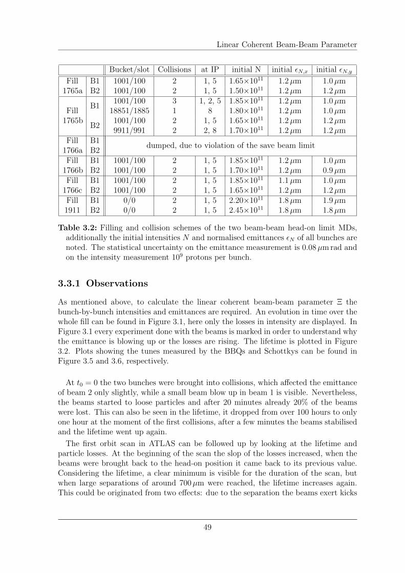
Linear Coherent Beam-Beam Parameter
Bucket/slot Collisions at IP initial N initial εN,x initial εN,y
Fill1765a
B1 1001/100 2 1, 5 1.65×10¹¹ 1.2µm 1.0µmB2 1001/100 2 1, 5 1.50×10¹¹ 1.2µm 1.2µm
Fill1765b
B11001/100 3 1, 2, 5 1.85×10¹¹ 1.2µm 1.0µm
18851/1885 1 8 1.80×10¹¹ 1.2µm 1.0µm
B21001/100 2 1, 5 1.65×10¹¹ 1.2µm 1.2µm9911/991 2 2, 8 1.70×10¹¹ 1.2µm 1.2µm
Fill1766a
B1dumped, due to violation of the save beam limit
B2Fill
1766bB1 1001/100 2 1, 5 1.85×10¹¹ 1.2µm 1.0µmB2 1001/100 2 1, 5 1.70×10¹¹ 1.2µm 0.9µm
Fill1766c
B1 1001/100 2 1, 5 1.85×10¹¹ 1.1µm 1.0µmB2 1001/100 2 1, 5 1.65×10¹¹ 1.2µm 1.2µm
Fill1911
B1 0/0 2 1, 5 2.20×10¹¹ 1.8µm 1.9µmB2 0/0 2 1, 5 2.45×10¹¹ 1.8µm 1.8µm
Table 3.2: Filling and collision schemes of the two beam-beam head-on limit MDs,additionally the initial intensities N and normalised emittances εN of all bunches arenoted. The statistical uncertainty on the emittance measurement is 0.08µm rad andon the intensity measurement 109 protons per bunch.
3.3.1 Observations
As mentioned above, to calculate the linear coherent beam-beam parameter Ξ thebunch-by-bunch intensities and emittances are required. An evolution in time over thewhole fill can be found in Figure 3.1, here only the losses in intensity are displayed. InFigure 3.1 every experiment done with the beams is marked in order to understand whythe emittance is blowing up or the losses are rising. The lifetime is plotted in Figure3.2. Plots showing the tunes measured by the BBQs and Schottkys can be found inFigure 3.5 and 3.6, respectively.
At t0 = 0 the two bunches were brought into collisions, which affected the emittanceof beam 2 only slightly, while a small beam blow up in beam 1 is visible. Nevertheless,the beams started to loose particles and after 20 minutes already 20% of the beamswere lost. This can also be seen in the lifetime, it dropped from over 100 hours to onlyone hour at the moment of the first collisions, after a few minutes the beams stabilisedand the lifetime went up again.
The first orbit scan in ATLAS can be followed up by looking at the lifetime andparticle losses. At the beginning of the scan the slop of the losses increased, when thebeams were brought back to the head-on position it came back to its previous value.Considering the lifetime, a clear minimum is visible for the duration of the scan, butwhen large separations of around 700µm were reached, the lifetime increases again.This could be originated from two effects: due to the separation the beams exert kicks
49
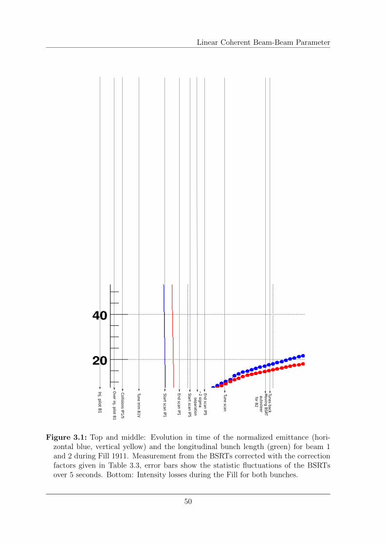
Linear Coherent Beam-Beam Parameter
Inj. pilot B1
Over inj. pilot B
1
Collisions IP1/5
Tune trim B
1V
Start scan IP1
End scan IP1
Start scan IP5
End scan IP5~
2 sigma
separation
Tune scan
Tunes backM
oving BSRT
autosteer for B
2
Figure 3.1: Top and middle: Evolution in time of the normalized emittance (hori-zontal blue, vertical yellow) and the longitudinal bunch length (green) for beam 1and 2 during Fill 1911. Measurement from the BSRTs corrected with the correctionfactors given in Table 3.3, error bars show the statistic fluctuations of the BSRTsover 5 seconds. Bottom: Intensity losses during the Fill for both bunches.
50
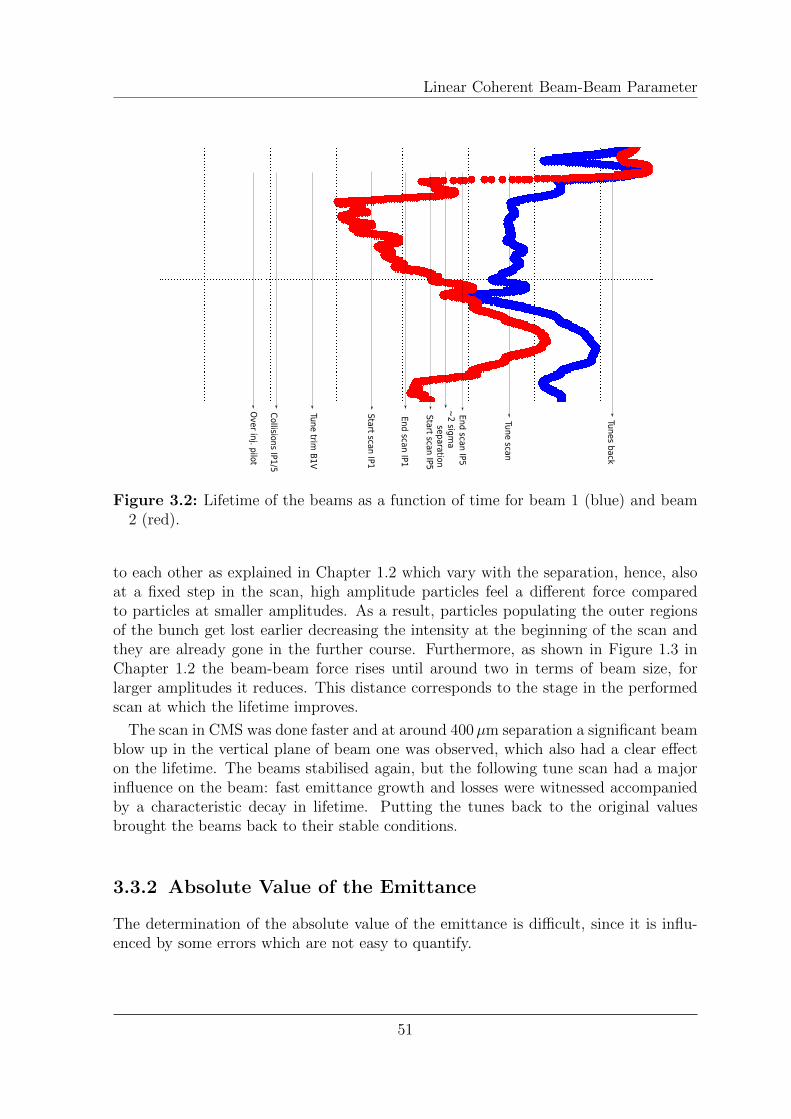
Linear Coherent Beam-Beam Parameter
Over inj. pilot
Collisions IP1/5
Tune trim B
1V
Start scan IP1
End scan IP1
Start scan IP5
End scan IP5~
2 sigma
separation
Tune scan
Tunes back
Figure 3.2: Lifetime of the beams as a function of time for beam 1 (blue) and beam2 (red).
to each other as explained in Chapter 1.2 which vary with the separation, hence, alsoat a fixed step in the scan, high amplitude particles feel a different force comparedto particles at smaller amplitudes. As a result, particles populating the outer regionsof the bunch get lost earlier decreasing the intensity at the beginning of the scan andthey are already gone in the further course. Furthermore, as shown in Figure 1.3 inChapter 1.2 the beam-beam force rises until around two in terms of beam size, forlarger amplitudes it reduces. This distance corresponds to the stage in the performedscan at which the lifetime improves.
The scan in CMS was done faster and at around 400µm separation a significant beamblow up in the vertical plane of beam one was observed, which also had a clear effecton the lifetime. The beams stabilised again, but the following tune scan had a majorinfluence on the beam: fast emittance growth and losses were witnessed accompaniedby a characteristic decay in lifetime. Putting the tunes back to the original valuesbrought the beams back to their stable conditions.
3.3.2 Absolute Value of the Emittance
The determination of the absolute value of the emittance is difficult, since it is influ-enced by some errors which are not easy to quantify.
51
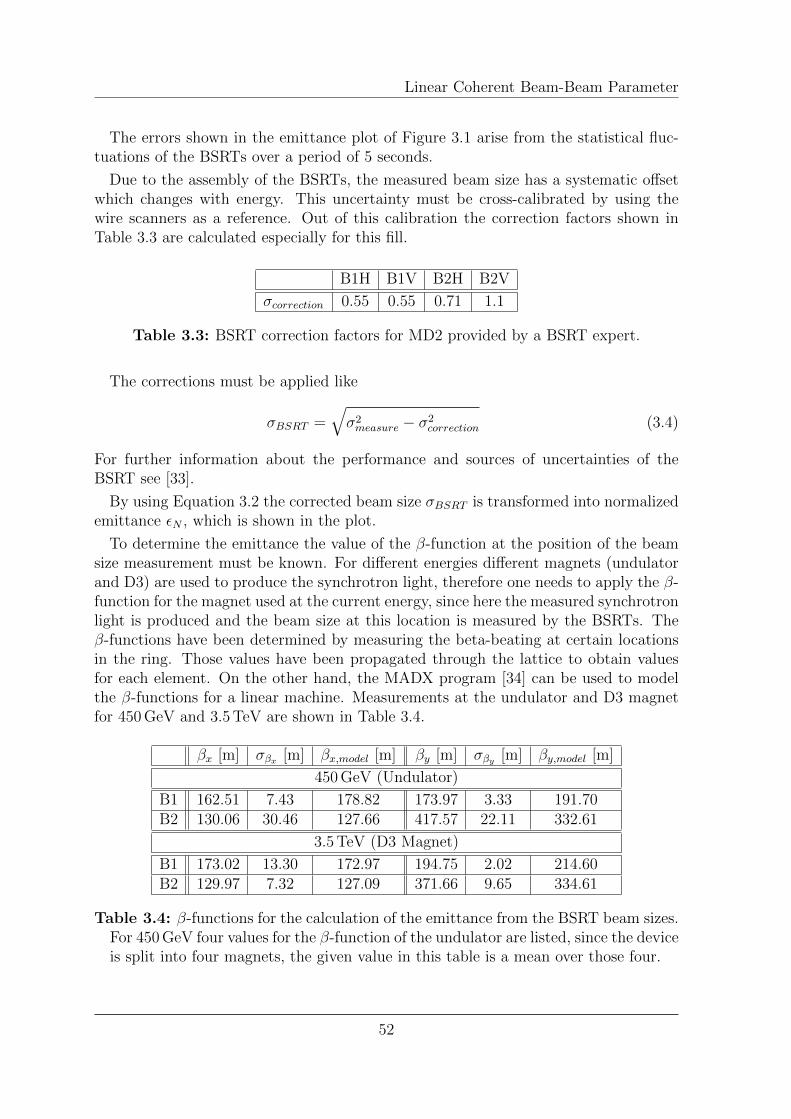
Linear Coherent Beam-Beam Parameter
The errors shown in the emittance plot of Figure 3.1 arise from the statistical fluc-tuations of the BSRTs over a period of 5 seconds.
Due to the assembly of the BSRTs, the measured beam size has a systematic offsetwhich changes with energy. This uncertainty must be cross-calibrated by using thewire scanners as a reference. Out of this calibration the correction factors shown inTable 3.3 are calculated especially for this fill.
B1H B1V B2H B2V
σcorrection 0.55 0.55 0.71 1.1
Table 3.3: BSRT correction factors for MD2 provided by a BSRT expert.
The corrections must be applied like
σBSRT =√σ2measure − σ2
correction (3.4)
For further information about the performance and sources of uncertainties of theBSRT see [33].
By using Equation 3.2 the corrected beam size σBSRT is transformed into normalizedemittance εN , which is shown in the plot.
To determine the emittance the value of the β-function at the position of the beamsize measurement must be known. For different energies different magnets (undulatorand D3) are used to produce the synchrotron light, therefore one needs to apply the β-function for the magnet used at the current energy, since here the measured synchrotronlight is produced and the beam size at this location is measured by the BSRTs. Theβ-functions have been determined by measuring the beta-beating at certain locationsin the ring. Those values have been propagated through the lattice to obtain valuesfor each element. On the other hand, the MADX program [34] can be used to modelthe β-functions for a linear machine. Measurements at the undulator and D3 magnetfor 450 GeV and 3.5 TeV are shown in Table 3.4.
βx [m] σβx [m] βx,model [m] βy [m] σβy [m] βy,model [m]
450 GeV (Undulator)
B1 162.51 7.43 178.82 173.97 3.33 191.70B2 130.06 30.46 127.66 417.57 22.11 332.61
3.5 TeV (D3 Magnet)
B1 173.02 13.30 172.97 194.75 2.02 214.60B2 129.97 7.32 127.09 371.66 9.65 334.61
Table 3.4: β-functions for the calculation of the emittance from the BSRT beam sizes.For 450 GeV four values for the β-function of the undulator are listed, since the deviceis split into four magnets, the given value in this table is a mean over those four.
52
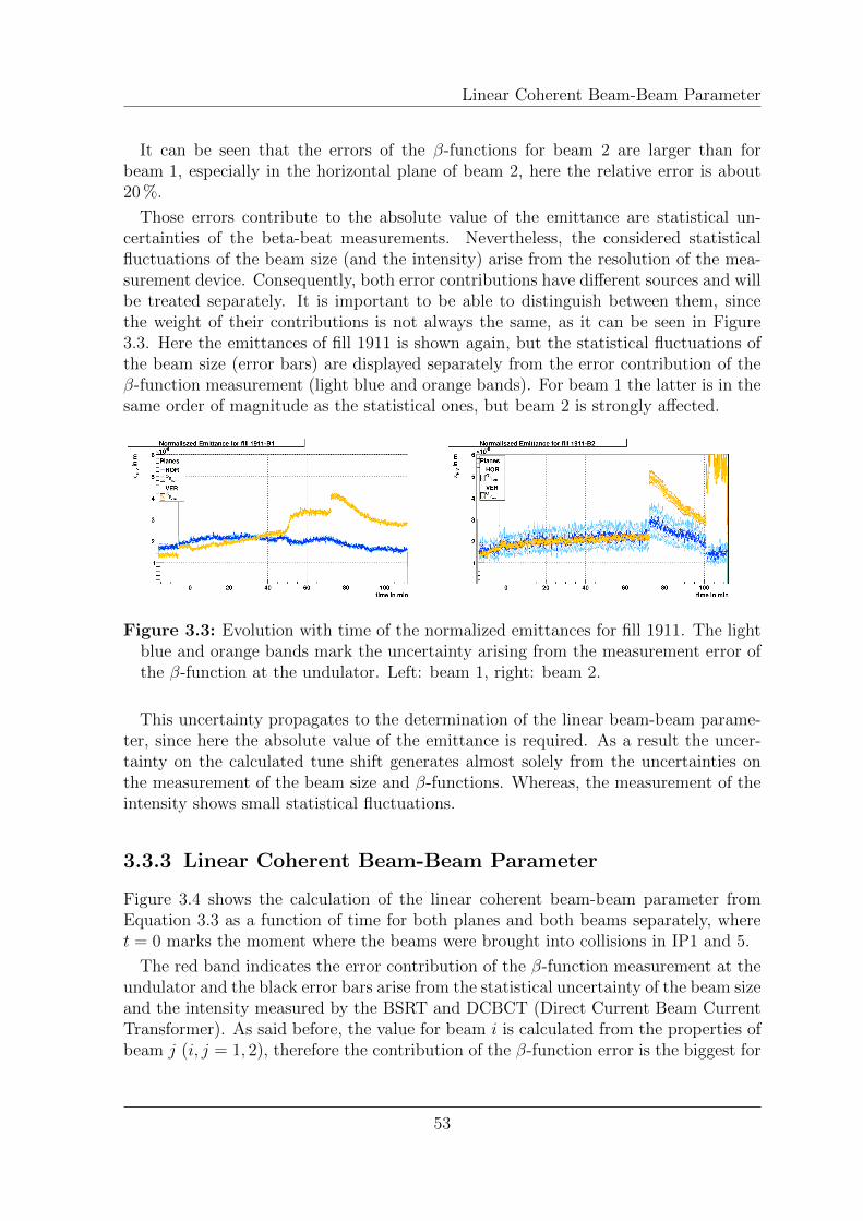
Linear Coherent Beam-Beam Parameter
It can be seen that the errors of the β-functions for beam 2 are larger than forbeam 1, especially in the horizontal plane of beam 2, here the relative error is about20 %.
Those errors contribute to the absolute value of the emittance are statistical un-certainties of the beta-beat measurements. Nevertheless, the considered statisticalfluctuations of the beam size (and the intensity) arise from the resolution of the mea-surement device. Consequently, both error contributions have different sources and willbe treated separately. It is important to be able to distinguish between them, sincethe weight of their contributions is not always the same, as it can be seen in Figure3.3. Here the emittances of fill 1911 is shown again, but the statistical fluctuations ofthe beam size (error bars) are displayed separately from the error contribution of theβ-function measurement (light blue and orange bands). For beam 1 the latter is in thesame order of magnitude as the statistical ones, but beam 2 is strongly affected.
Figure 3.3: Evolution with time of the normalized emittances for fill 1911. The lightblue and orange bands mark the uncertainty arising from the measurement error ofthe β-function at the undulator. Left: beam 1, right: beam 2.
This uncertainty propagates to the determination of the linear beam-beam parame-ter, since here the absolute value of the emittance is required. As a result the uncer-tainty on the calculated tune shift generates almost solely from the uncertainties onthe measurement of the beam size and β-functions. Whereas, the measurement of theintensity shows small statistical fluctuations.
3.3.3 Linear Coherent Beam-Beam Parameter
Figure 3.4 shows the calculation of the linear coherent beam-beam parameter fromEquation 3.3 as a function of time for both planes and both beams separately, wheret = 0 marks the moment where the beams were brought into collisions in IP1 and 5.
The red band indicates the error contribution of the β-function measurement at theundulator and the black error bars arise from the statistical uncertainty of the beam sizeand the intensity measured by the BSRT and DCBCT (Direct Current Beam CurrentTransformer). As said before, the value for beam i is calculated from the properties ofbeam j (i, j = 1, 2), therefore the contribution of the β-function error is the biggest for
53
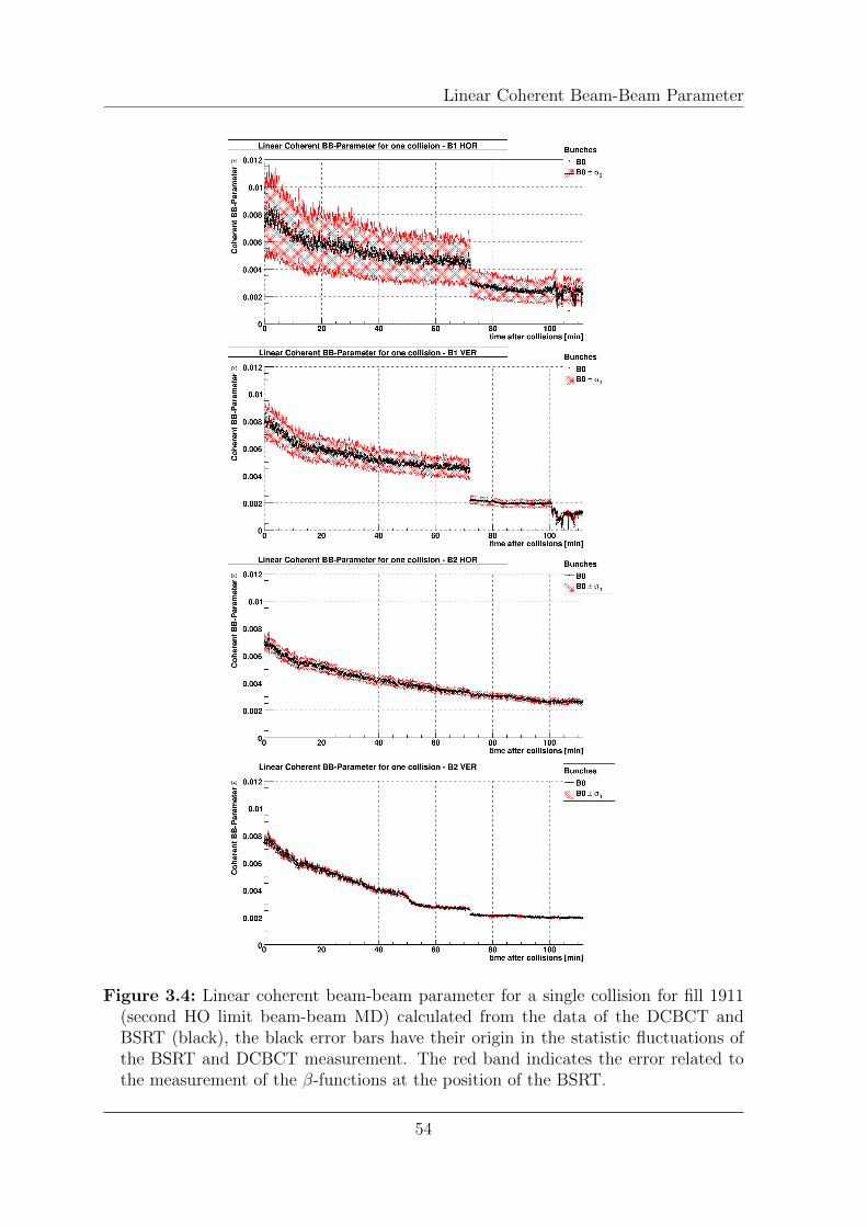
Linear Coherent Beam-Beam Parameter
Figure 3.4: Linear coherent beam-beam parameter for a single collision for fill 1911(second HO limit beam-beam MD) calculated from the data of the DCBCT andBSRT (black), the black error bars have their origin in the statistic fluctuations ofthe BSRT and DCBCT measurement. The red band indicates the error related tothe measurement of the β-functions at the position of the BSRT.
54
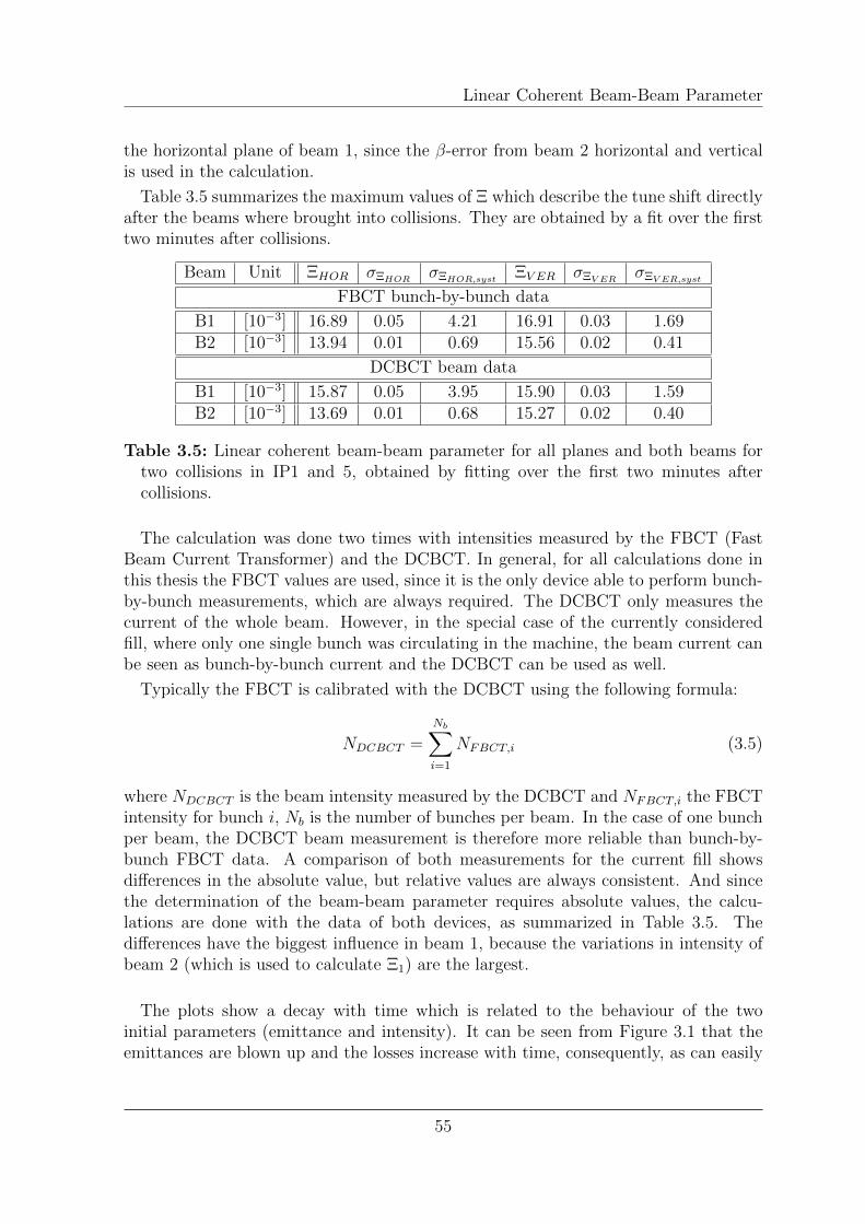
Linear Coherent Beam-Beam Parameter
the horizontal plane of beam 1, since the β-error from beam 2 horizontal and verticalis used in the calculation.
Table 3.5 summarizes the maximum values of Ξ which describe the tune shift directlyafter the beams where brought into collisions. They are obtained by a fit over the firsttwo minutes after collisions.
Beam Unit ΞHOR σΞHORσΞHOR,syst
ΞV ER σΞV ERσΞV ER,syst
FBCT bunch-by-bunch data
B1 [10−3] 16.89 0.05 4.21 16.91 0.03 1.69B2 [10−3] 13.94 0.01 0.69 15.56 0.02 0.41
DCBCT beam data
B1 [10−3] 15.87 0.05 3.95 15.90 0.03 1.59B2 [10−3] 13.69 0.01 0.68 15.27 0.02 0.40
Table 3.5: Linear coherent beam-beam parameter for all planes and both beams fortwo collisions in IP1 and 5, obtained by fitting over the first two minutes aftercollisions.
The calculation was done two times with intensities measured by the FBCT (FastBeam Current Transformer) and the DCBCT. In general, for all calculations done inthis thesis the FBCT values are used, since it is the only device able to perform bunch-by-bunch measurements, which are always required. The DCBCT only measures thecurrent of the whole beam. However, in the special case of the currently consideredfill, where only one single bunch was circulating in the machine, the beam current canbe seen as bunch-by-bunch current and the DCBCT can be used as well.
Typically the FBCT is calibrated with the DCBCT using the following formula:
NDCBCT =
Nb∑i=1
NFBCT,i (3.5)
where NDCBCT is the beam intensity measured by the DCBCT and NFBCT,i the FBCTintensity for bunch i, Nb is the number of bunches per beam. In the case of one bunchper beam, the DCBCT beam measurement is therefore more reliable than bunch-by-bunch FBCT data. A comparison of both measurements for the current fill showsdifferences in the absolute value, but relative values are always consistent. And sincethe determination of the beam-beam parameter requires absolute values, the calcu-lations are done with the data of both devices, as summarized in Table 3.5. Thedifferences have the biggest influence in beam 1, because the variations in intensity ofbeam 2 (which is used to calculate Ξ1) are the largest.
The plots show a decay with time which is related to the behaviour of the twoinitial parameters (emittance and intensity). It can be seen from Figure 3.1 that theemittances are blown up and the losses increase with time, consequently, as can easily
55

Linear Coherent Beam-Beam Parameter
be verified from Equation 3.3, Ξ must decrease.
The big jump at around minute 70 corresponds to a step in the performed tune scan,which hit a resonance and caused a huge beam blow up and fast losses in intensity.Beam 2 vertical also suffers from the emittance increase in the vertical plane of beam1 provoked by the orbit scan in IP5.
The increase in emittance and the reduction of intensity with time implies that thebeam-beam force decreases with time as well, i.e. the tune shift with respect to theinitial tunes before collisions becomes smaller, what on the other hand shows thatthe beam-beam effect is maximal for high brilliant beams, small emittances and highintensities.
3.3.4 Tune Shift from Tune Measurements
During the fill the tunes were measured by the Schottkys (Figure 3.6) and the Base-Band Tune measurement system (BBQ, Figure 3.5). Unfortunately the measurementsare very noisy.
The data taken by the BBQ is unsuitable for the calculation of the tune shift, as itis illustrated in Figure 3.5. It shows a big spread between single measurements as longas the transverse damper is on. Among other things, the damper is used to preventfor coherent oscillations, thus it excites the beam with a variable frequency whichsuppresses undesired oscillations. Unfortunately, this frequency is close to the tuneand since the BBQ works on a peak finder basis it sometimes just finds the damperfrequency instead of the tune.
Later, after the second orbit scan in IP5 the damper was switched off and the dataimmediately becomes practical. But at the moment were the beams were brought intointeraction it is impossible to extract a value for the tune shift.
Figure 3.5: Evolution in time of the tunes measured by the BBQs (horizontal blue,vertical yellow) during fill 1911. Left: beam 1, right: beam 2.
In principle the Schottky monitor measures a noise signal arising from the Schottkynoise of the moving particles. It uses the difference signal between two pick-ups tofilter the coherent signal, which overlies the desired incoherent one. The device is notyet fully commissioned, so that it is sometimes difficult to obtain a clean signal. The
56
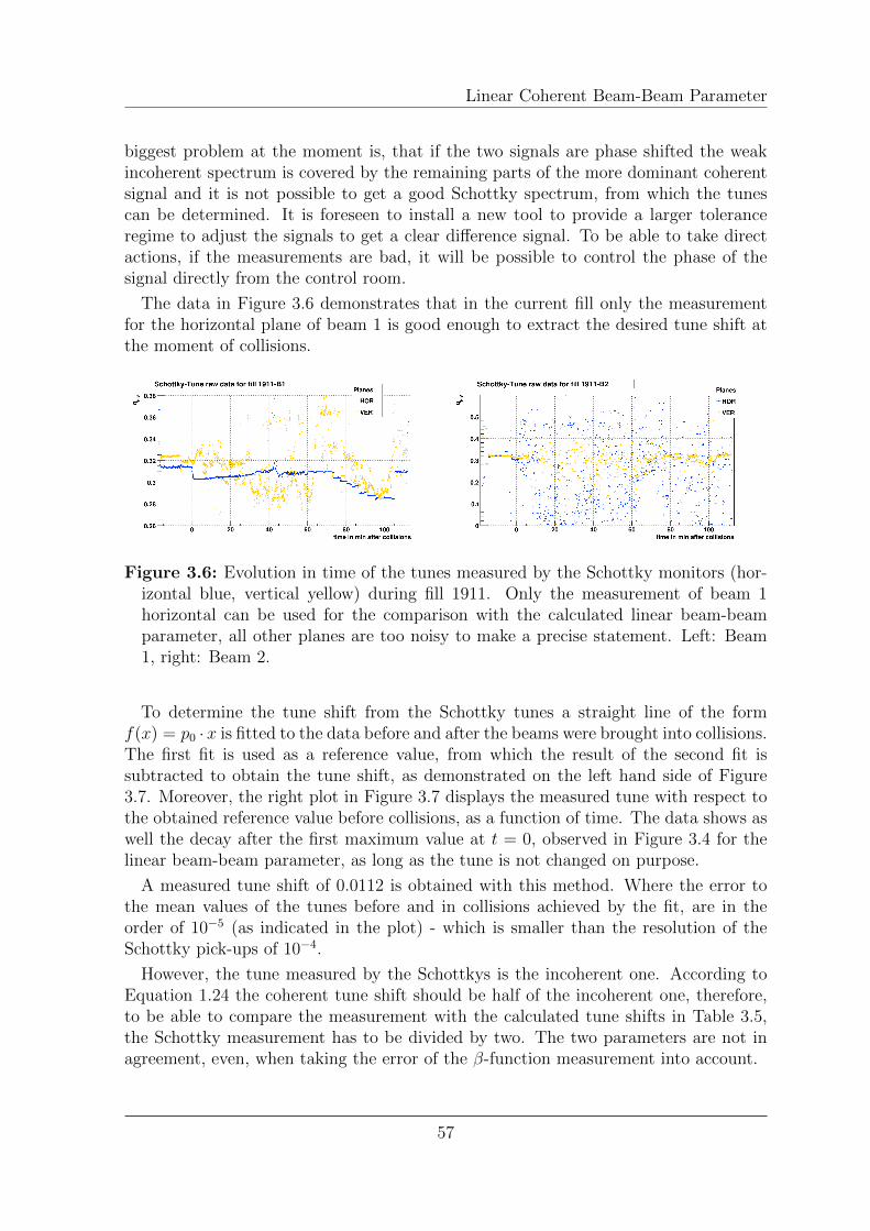
Linear Coherent Beam-Beam Parameter
biggest problem at the moment is, that if the two signals are phase shifted the weakincoherent spectrum is covered by the remaining parts of the more dominant coherentsignal and it is not possible to get a good Schottky spectrum, from which the tunescan be determined. It is foreseen to install a new tool to provide a larger toleranceregime to adjust the signals to get a clear difference signal. To be able to take directactions, if the measurements are bad, it will be possible to control the phase of thesignal directly from the control room.
The data in Figure 3.6 demonstrates that in the current fill only the measurementfor the horizontal plane of beam 1 is good enough to extract the desired tune shift atthe moment of collisions.
Figure 3.6: Evolution in time of the tunes measured by the Schottky monitors (hor-izontal blue, vertical yellow) during fill 1911. Only the measurement of beam 1horizontal can be used for the comparison with the calculated linear beam-beamparameter, all other planes are too noisy to make a precise statement. Left: Beam1, right: Beam 2.
To determine the tune shift from the Schottky tunes a straight line of the formf(x) = p0 ·x is fitted to the data before and after the beams were brought into collisions.The first fit is used as a reference value, from which the result of the second fit issubtracted to obtain the tune shift, as demonstrated on the left hand side of Figure3.7. Moreover, the right plot in Figure 3.7 displays the measured tune with respect tothe obtained reference value before collisions, as a function of time. The data shows aswell the decay after the first maximum value at t = 0, observed in Figure 3.4 for thelinear beam-beam parameter, as long as the tune is not changed on purpose.
A measured tune shift of 0.0112 is obtained with this method. Where the error tothe mean values of the tunes before and in collisions achieved by the fit, are in theorder of 10−5 (as indicated in the plot) - which is smaller than the resolution of theSchottky pick-ups of 10−4.
However, the tune measured by the Schottkys is the incoherent one. According toEquation 1.24 the coherent tune shift should be half of the incoherent one, therefore,to be able to compare the measurement with the calculated tune shifts in Table 3.5,the Schottky measurement has to be divided by two. The two parameters are not inagreement, even, when taking the error of the β-function measurement into account.
57
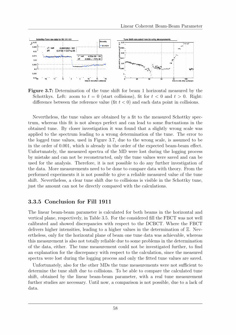
Linear Coherent Beam-Beam Parameter
Figure 3.7: Determination of the tune shift for beam 1 horizontal measured by theSchottkys. Left: zoom to t = 0 (start collisions), fit for t < 0 and t > 0. Right:difference between the reference value (fit t < 0) and each data point in collisions.
Nevertheless, the tune values are obtained by a fit to the measured Schottky spec-trum, whereas this fit is not always perfect and can lead to some fluctuations in theobtained tune. By closer investigation it was found that a slightly wrong scale wasapplied to the spectrum leading to a wrong determination of the tune. The error tothe logged tune values, used in Figure 3.7, due to the wrong scale, is assumed to bein the order of 0.001, which is already in the order of the expected beam-beam effect.Unfortunately, the measured spectra of the MD were lost during the logging processby mistake and can not be reconstructed, only the tune values were saved and can beused for the analysis. Therefore, it is not possible to do any further investigation ofthe data. More measurements need to be done to compare data with theory. From theperformed experiments it is not possible to give a reliable measured value of the tuneshift. Nevertheless, a clear tune shift due to collisions is visible in the Schottky tune,just the amount can not be directly compared with the calculations.
3.3.5 Conclusion for Fill 1911
The linear beam-beam parameter is calculated for both beams in the horizontal andvertical plane, respectively, in Table 3.5. For the considered fill the FBCT was not wellcalibrated and showed discrepancies with respect to the DCBCT. Where the FBCTdelivers higher intensities, leading to a higher values in the determination of Ξ. Nev-ertheless, only for the horizontal plane of beam one tune data was achievable, whereasthis measurement is also not totally reliable due to some problems in the determinationof the data, either. The tune measurement could not be investigated further, to findan explanation for the discrepancy with respect to the calculation, since the measuredspectra were lost during the logging process and only the fitted tune values are saved.
Unfortunately, also for the other MDs the tune measurements were not sufficient todetermine the tune shift due to collisions. To be able to compare the calculated tuneshift, obtained by the linear beam-beam parameter, with a real tune measurementfurther studies are necessary. Until now, a comparison is not possible, due to a lack ofdata.
58
Linear Coherent Beam-Beam Parameter
3.4 Analysis of Further Data
The same experiment as discussed in the previous chapter was done a second time forbunches with different emittances and intensities in fill 1765 and 1766. The obtainedvalues for the linear coherent beam-beam parameter are listed in Table 3.6.
Contrary to fill 1911 in fill 1765a and 1766b/c the beams were brought into collisionsin IP1 and 5 with a significant time difference, consequently the linear beam-beamparameter was calculated at two different times per fill. First when IP1 was collapsed(t0 = 0) and secondly when the bumps in IP5 were closed (t1 > 0). In the second case,the value obtained from the data was multiplied by two to reflect the overall tune shift,since now two collisions are present. This is the reason why the value at t1 is biggerthan at t0, but it is not twice the amount, because in the meantime the bunches lostparticles and blew up in emittance.
As it can be seen from Table 3.2 the initial conditions for both beams in fill 1765a,bunch 100 in fill 1765b beam 2 and beam 2 of fill 1766c are comparable, thereforethey should exert similar forces to the opposite beam. The small discrepancies in theresults arise from different reactions when the bunches were brought into collisionsin the different IPs. For fill 1765a a beam blow up to around 2.2µm was observedwhen collisions started in ATLAS, whereas the beams were only slightly affected bythe collisions in CMS. For bunch 100 of fill 1765b a similar behaviour was observed.In both cases the vertical plane suffered more, consequently the calculated parameterbecomes smaller in that plane compared to the horizontal one. But after the first blowup the growth rate of the horizontal plane was faster in all cases, hence the beam-beameffect became less important in the horizontal plane when collisions started in IP5. Theeffect on fill 1766c is larger, because the bunches were relatively stable in interactionsand did not experience a significant blow up nor great losses.
As well bunch 100 of beam 1 in fill 1765b, fill 1766b and beam 1 of fill 1766c hadcomparable initial parameters. For beam 1 of the first fill a similar behaviour as forbeam 2 is observed: beam blow up mainly in the vertical plane and drastic increase inlosses due to collisions in IP1, collisions in IP5 bring no significant changes.
In case of fill 1766b, the vertical emittance was the smallest when the bunches werebrought into collisions in the first IP, which also does not seem to affect the emittancegrowth and intensity losses significantly. Nevertheless during luminosity optimizationa great emittance blow up was seen in the vertical plane. In the horizontal plane theincrease was smaller. It was suggested that this blow up was caused by small amplitude(core) particles of the beam being close to the 10th order resonances. Significant losseshave not been observed. Due to the large emittances when collisions started in IP5,the beam-beam tune shift is smaller for two collisions than for one.
Fill 1766c shows a stable behaviour when the beams are brought into collisions, whilethe horizontal plane growth faster than the vertical one and beam 1 experience lossesof about 10% when it starts to collide in IP5.
59
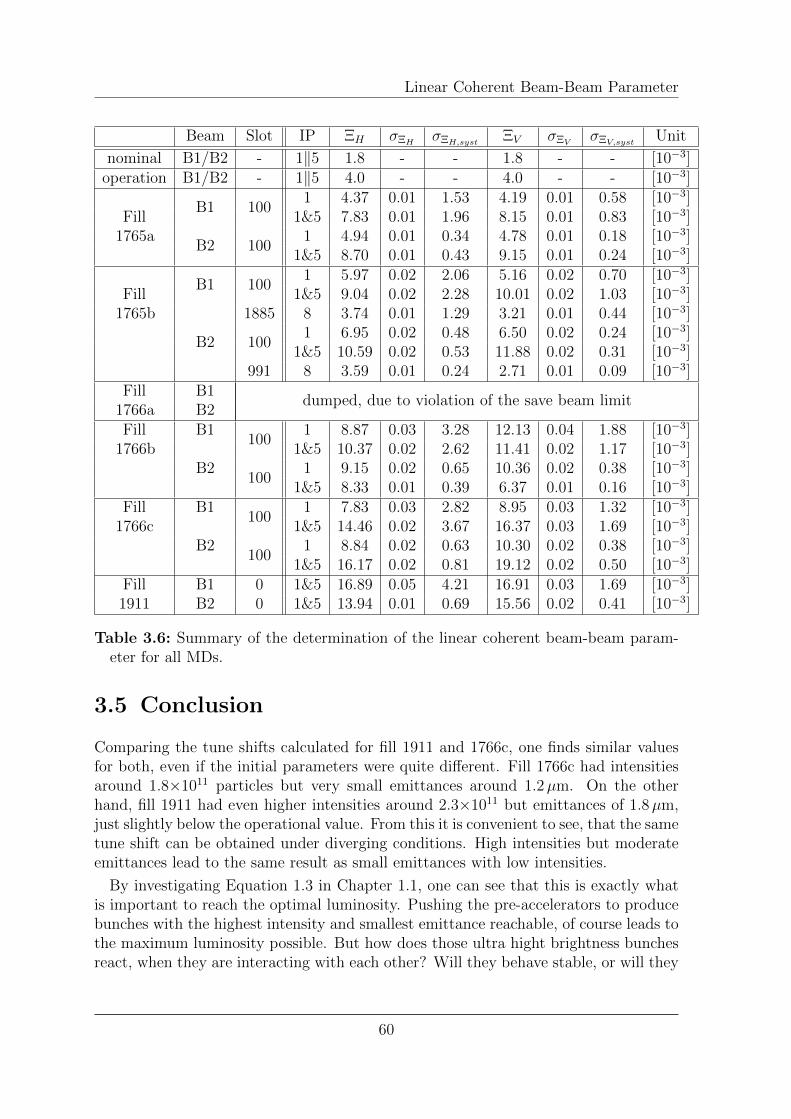
Linear Coherent Beam-Beam Parameter
Beam Slot IP ΞH σΞHσΞH,syst
ΞV σΞVσΞV,syst
Unit
nominal B1/B2 - 1‖5 1.8 - - 1.8 - - [10−3]operation B1/B2 - 1‖5 4.0 - - 4.0 - - [10−3]
Fill1765a
B1 1001 4.37 0.01 1.53 4.19 0.01 0.58 [10−3]
1&5 7.83 0.01 1.96 8.15 0.01 0.83 [10−3]
B2 1001 4.94 0.01 0.34 4.78 0.01 0.18 [10−3]
1&5 8.70 0.01 0.43 9.15 0.01 0.24 [10−3]
Fill1765b
B1 1001 5.97 0.02 2.06 5.16 0.02 0.70 [10−3]
1&5 9.04 0.02 2.28 10.01 0.02 1.03 [10−3]1885 8 3.74 0.01 1.29 3.21 0.01 0.44 [10−3]
B2 1001 6.95 0.02 0.48 6.50 0.02 0.24 [10−3]
1&5 10.59 0.02 0.53 11.88 0.02 0.31 [10−3]991 8 3.59 0.01 0.24 2.71 0.01 0.09 [10−3]
Fill1766a
B1dumped, due to violation of the save beam limit
B2Fill
1766bB1
1001 8.87 0.03 3.28 12.13 0.04 1.88 [10−3]
1&5 10.37 0.02 2.62 11.41 0.02 1.17 [10−3]B2
1001 9.15 0.02 0.65 10.36 0.02 0.38 [10−3]
1&5 8.33 0.01 0.39 6.37 0.01 0.16 [10−3]Fill
1766cB1
1001 7.83 0.03 2.82 8.95 0.03 1.32 [10−3]
1&5 14.46 0.02 3.67 16.37 0.03 1.69 [10−3]B2
1001 8.84 0.02 0.63 10.30 0.02 0.38 [10−3]
1&5 16.17 0.02 0.81 19.12 0.02 0.50 [10−3]Fill1911
B1 0 1&5 16.89 0.05 4.21 16.91 0.03 1.69 [10−3]B2 0 1&5 13.94 0.01 0.69 15.56 0.02 0.41 [10−3]
Table 3.6: Summary of the determination of the linear coherent beam-beam param-eter for all MDs.
3.5 Conclusion
Comparing the tune shifts calculated for fill 1911 and 1766c, one finds similar valuesfor both, even if the initial parameters were quite different. Fill 1766c had intensitiesaround 1.8×10¹¹ particles but very small emittances around 1.2µm. On the otherhand, fill 1911 had even higher intensities around 2.3×10¹¹ but emittances of 1.8µm,just slightly below the operational value. From this it is convenient to see, that the sametune shift can be obtained under diverging conditions. High intensities but moderateemittances lead to the same result as small emittances with low intensities.
By investigating Equation 1.3 in Chapter 1.1, one can see that this is exactly whatis important to reach the optimal luminosity. Pushing the pre-accelerators to producebunches with the highest intensity and smallest emittance reachable, of course leads tothe maximum luminosity possible. But how does those ultra hight brightness bunchesreact, when they are interacting with each other? Will they behave stable, or will they
60
Linear Coherent Beam-Beam Parameter
blow up, loose particles and decrease in lifetime? This is one of the most importantquestions to be clarified for the luminosity upgrade of LHC to be able to reach theoptimum in luminosity.
As well for the daily operation it is important to know what conditions are the easiestones to handle in the LHC and if the one or the other is more convenient to be producedby the pre-accelerators.
The aim of the experiments discussed in this chapter was to see how far one canpush the brightness of the beams without getting into trouble in terms of blow up,losses and lifetime problems. In fill 1911 we already saw related beam blow up andparticle losses, but a final limit is not yet been found. Moreover, those experimentsdiscussed where only done at injection energy. It is important to do further analysis athigh energies to confirm a stable behaviour under normal running conditions, as well.
However, the tune shifts achieved in the experiments exceed the nominal value byalmost a factor of 5 and the value reached in normal operation already by a factor of2. This is an unexpected but desired result of which nobody had ever thought duringthe construction of LHC.
61

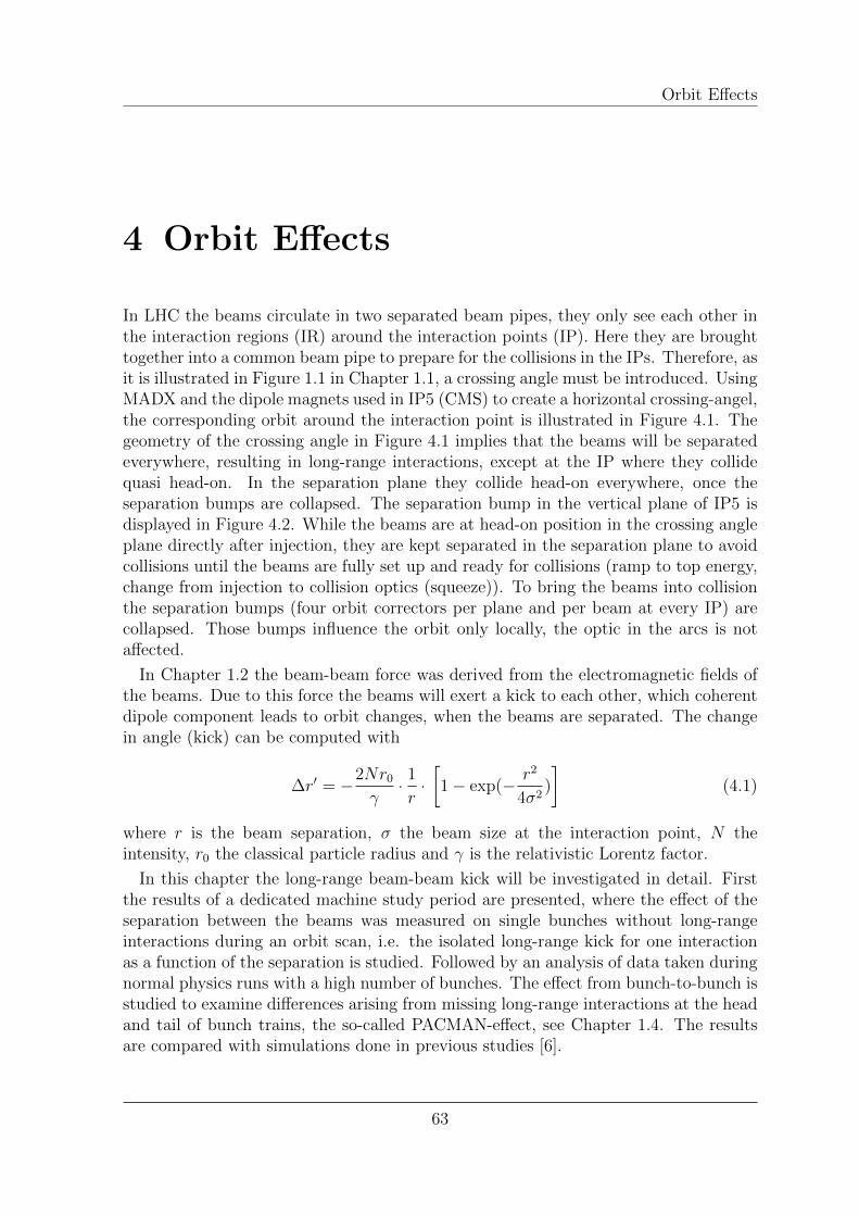
Orbit Effects
4 Orbit Effects
In LHC the beams circulate in two separated beam pipes, they only see each other inthe interaction regions (IR) around the interaction points (IP). Here they are broughttogether into a common beam pipe to prepare for the collisions in the IPs. Therefore, asit is illustrated in Figure 1.1 in Chapter 1.1, a crossing angle must be introduced. UsingMADX and the dipole magnets used in IP5 (CMS) to create a horizontal crossing-angel,the corresponding orbit around the interaction point is illustrated in Figure 4.1. Thegeometry of the crossing angle in Figure 4.1 implies that the beams will be separatedeverywhere, resulting in long-range interactions, except at the IP where they collidequasi head-on. In the separation plane they collide head-on everywhere, once theseparation bumps are collapsed. The separation bump in the vertical plane of IP5 isdisplayed in Figure 4.2. While the beams are at head-on position in the crossing angleplane directly after injection, they are kept separated in the separation plane to avoidcollisions until the beams are fully set up and ready for collisions (ramp to top energy,change from injection to collision optics (squeeze)). To bring the beams into collisionthe separation bumps (four orbit correctors per plane and per beam at every IP) arecollapsed. Those bumps influence the orbit only locally, the optic in the arcs is notaffected.
In Chapter 1.2 the beam-beam force was derived from the electromagnetic fields ofthe beams. Due to this force the beams will exert a kick to each other, which coherentdipole component leads to orbit changes, when the beams are separated. The changein angle (kick) can be computed with
∆r′ = −2Nr0
γ·1
r·[1− exp(− r2
4σ2)
](4.1)
where r is the beam separation, σ the beam size at the interaction point, N theintensity, r0 the classical particle radius and γ is the relativistic Lorentz factor.
In this chapter the long-range beam-beam kick will be investigated in detail. Firstthe results of a dedicated machine study period are presented, where the effect of theseparation between the beams was measured on single bunches without long-rangeinteractions during an orbit scan, i.e. the isolated long-range kick for one interactionas a function of the separation is studied. Followed by an analysis of data taken duringnormal physics runs with a high number of bunches. The effect from bunch-to-bunch isstudied to examine differences arising from missing long-range interactions at the headand tail of bunch trains, the so-called PACMAN-effect, see Chapter 1.4. The resultsare compared with simulations done in previous studies [6].
63

Orbit Effects
Figure 4.1: Orbit of beam 1 around CMS. Four corrector magnets are used for the cre-ation of a horizontal crossing-angle. At 3.5 TeV the corresponding angle is 240µrad.The top row shows the lattice in the considered sector: centred squares indicatebending magnets, lowered (upper) ones defocusing (focusing) quadrupoles. This isa MADX simulation.
4.1 Long-Range Beam-Beam Kick
In the same MD as mentioned in the previous chapter (fill 1911), with only one bunchcirculating per beam, a horizontal orbit scan was performed in ATLAS (IP1) and avertical one in CMS (IP5).
When only one bunch is present per beam, influence arising from parasitic encounterswith other bunches (long-range) are avoided. Moreover, the scans were done in theseparation plane to separate the barycentres of the bunches and not just shift thecentre of the interaction away from the IP, as it would be the case for a separation inthe crossing plane. To avoid additional effects arising from the trim of the separationbumps (e.g. the non-closure effect: due to magnet errors the bumps does not closeperfectly, leaving an offset or angle which causes an additional oscillation around thering), only beam one was moved and beam two was untouched. In this way beam twois only perturbed by the beam-beam kick. This set up provides the cleanest signalavailable to measure the orbit kick due to the beam-beam force when the beams areseparated.
After a luminosity optimization, where the beams were brought to their total over-lap position in the IPs, the scans were done in steps of 100µm, which corresponds
64
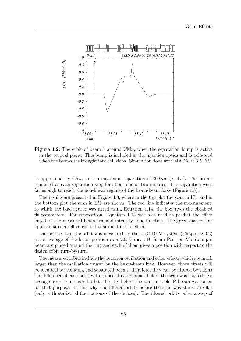
Orbit Effects
Figure 4.2: The orbit of beam 1 around CMS, when the separation bump is activein the vertical plane. This bump is included in the injection optics and is collapsedwhen the beams are brought into collisions. Simulation done with MADX at 3.5 TeV.
to approximately 0.5σ, until a maximum separation of 800µm (∼ 4σ). The beamsremained at each separation step for about one or two minutes. The separation wentfar enough to reach the non-linear regime of the beam-beam force (Figure 1.3).
The results are presented in Figure 4.3, where in the top plot the scan in IP1 and inthe bottom plot the scan in IP5 are shown. The red line indicates the measurement,to which the black curve was fitted using Equation 1.14, the box gives the obtainedfit parameters. For comparison, Equation 1.14 was also used to predict the effectbased on the measured beam size and intensity, blue function. The green dashed lineapproximates a self-consistent treatment of the effect.
During the scan the orbit was measured by the LHC BPM system (Chapter 2.3.2)as an average of the beam position over 225 turns. 516 Beam Position Monitors perbeam are placed around the ring and each of them gives a position with respect to thedesign orbit turn-by-turn.
The measured orbits include the betatron oscillation and other effects which are muchlarger than the oscillation caused by the beam-beam kick. However, those offsets willbe identical for colliding and separated beams, therefore, they can be filtered by takingthe difference of each orbit with respect to a reference before the scan was started. Anaverage over 10 measured orbits directly before the scan in each IP began was takenfor that purpose. In this why, the filtered orbits before the scan was stared are flat(only with statistical fluctuations of the devices). The filtered orbits, after a step of
65
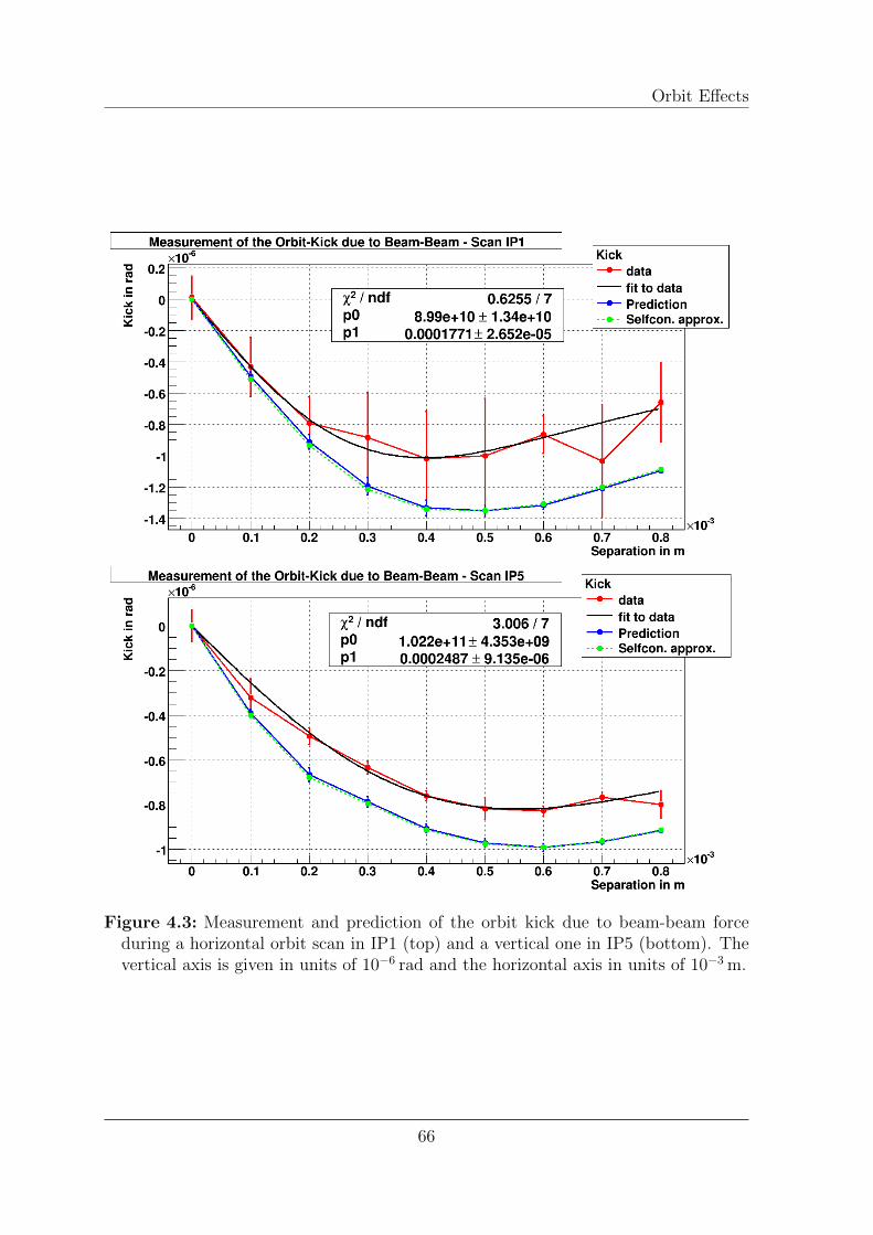
Orbit Effects
Figure 4.3: Measurement and prediction of the orbit kick due to beam-beam forceduring a horizontal orbit scan in IP1 (top) and a vertical one in IP5 (bottom). Thevertical axis is given in units of 10−6 rad and the horizontal axis in units of 10−3 m.
66
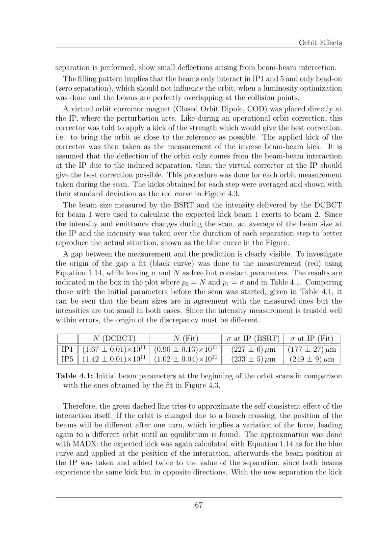
Orbit Effects
separation is performed, show small deflections arising from beam-beam interaction.
The filling pattern implies that the beams only interact in IP1 and 5 and only head-on(zero separation), which should not influence the orbit, when a luminosity optimizationwas done and the beams are perfectly overlapping at the collision points.
A virtual orbit corrector magnet (Closed Orbit Dipole, COD) was placed directly atthe IP, where the perturbation acts. Like during an operational orbit correction, thiscorrector was told to apply a kick of the strength which would give the best correction,i.e. to bring the orbit as close to the reference as possible. The applied kick of thecorrector was then taken as the measurement of the inverse beam-beam kick. It isassumed that the deflection of the orbit only comes from the beam-beam interactionat the IP due to the induced separation, thus, the virtual corrector at the IP shouldgive the best correction possible. This procedure was done for each orbit measurementtaken during the scan. The kicks obtained for each step were averaged and shown withtheir standard deviation as the red curve in Figure 4.3.
The beam size measured by the BSRT and the intensity delivered by the DCBCTfor beam 1 were used to calculate the expected kick beam 1 exerts to beam 2. Sincethe intensity and emittance changes during the scan, an average of the beam size atthe IP and the intensity was taken over the duration of each separation step to betterreproduce the actual situation, shown as the blue curve in the Figure.
A gap between the measurement and the prediction is clearly visible. To investigatethe origin of the gap a fit (black curve) was done to the measurement (red) usingEquation 1.14, while leaving σ and N as free but constant parameters. The results areindicated in the box in the plot where p0 = N and p1 = σ and in Table 4.1. Comparingthose with the initial parameters before the scan was started, given in Table 4.1, itcan be seen that the beam sizes are in agreement with the measured ones but theintensities are too small in both cases. Since the intensity measurement is trusted wellwithin errors, the origin of the discrepancy must be different.
N (DCBCT) N (Fit) σ at IP (BSRT) σ at IP (Fit)
IP1 (1.67 ± 0.01)×1011 (0.90 ± 0.13)×1011 (227 ± 6)µm (177 ± 27)µmIP5 (1.42 ± 0.01)×1011 (1.02 ± 0.04)×1011 (233 ± 5)µm (249 ± 9)µm
Table 4.1: Initial beam parameters at the beginning of the orbit scans in comparisonwith the ones obtained by the fit in Figure 4.3.
Therefore, the green dashed line tries to approximate the self-consistent effect of theinteraction itself. If the orbit is changed due to a bunch crossing, the position of thebeams will be different after one turn, which implies a variation of the force, leadingagain to a different orbit until an equilibrium is found. The approximation was donewith MADX: the expected kick was again calculated with Equation 1.14 as for the bluecurve and applied at the position of the interaction, afterwards the beam position atthe IP was taken and added twice to the value of the separation, since both beamsexperience the same kick but in opposite directions. With the new separation the kick
67
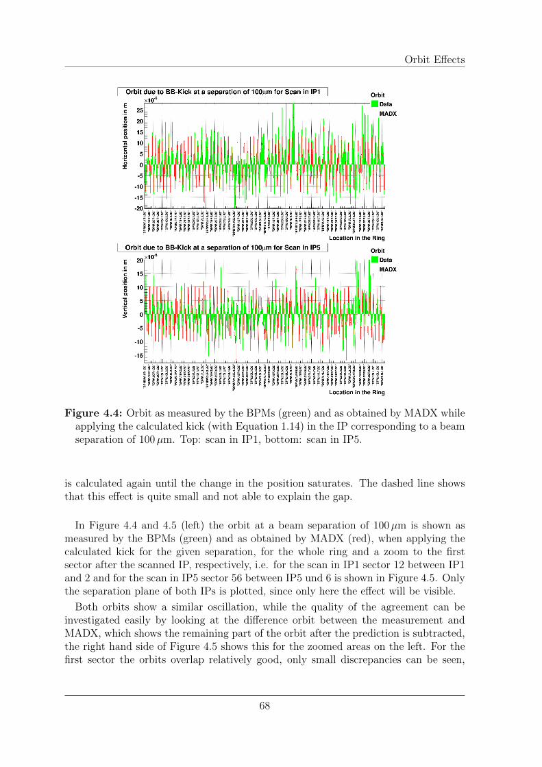
Orbit Effects
Figure 4.4: Orbit as measured by the BPMs (green) and as obtained by MADX whileapplying the calculated kick (with Equation 1.14) in the IP corresponding to a beamseparation of 100µm. Top: scan in IP1, bottom: scan in IP5.
is calculated again until the change in the position saturates. The dashed line showsthat this effect is quite small and not able to explain the gap.
In Figure 4.4 and 4.5 (left) the orbit at a beam separation of 100µm is shown asmeasured by the BPMs (green) and as obtained by MADX (red), when applying thecalculated kick for the given separation, for the whole ring and a zoom to the firstsector after the scanned IP, respectively, i.e. for the scan in IP1 sector 12 between IP1and 2 and for the scan in IP5 sector 56 between IP5 und 6 is shown in Figure 4.5. Onlythe separation plane of both IPs is plotted, since only here the effect will be visible.
Both orbits show a similar oscillation, while the quality of the agreement can beinvestigated easily by looking at the difference orbit between the measurement andMADX, which shows the remaining part of the orbit after the prediction is subtracted,the right hand side of Figure 4.5 shows this for the zoomed areas on the left. For thefirst sector the orbits overlap relatively good, only small discrepancies can be seen,
68
Orbit Effects
Figure 4.5: Left: Orbit as measured by the BPMs (green) and as obtained by MADXwhile applying the calculated kick (with Equation 1.14) in the IP corresponding toa beam separation of 100µm. On the right a difference of both orbits is illustrated.All plots show a zoom to the first sector after the scanned IP. Top row: horizontalseparation in IP1, bottom: vertical separation in IP5.
which, as the difference orbit indicates, are in the order of ± 5 to 6µm, correspond-ing to the noise level of the BPMs (see Chapter 4.2.2). However, as the oscillationpropagates through the ring some BPMs show bigger differences and going to largerseparations (above 500µm) some sectors become very bad and give differences of morethan 15µm. Moreover, sometimes it seems that an oscillation remains in the differenceorbit. The corresponding separation, where those additional perturbations becomestronger, appears to be around the maximum of the beam-beam kick, after which thekick becomes smaller with increasing distance between the beams.
Nevertheless, it is known that the signal of the BPMs depend on the intensity of thebeam, that’s why they are operated in a low or high sensitivity mode depending onthe bunch intensity, but also the position of the beam is important for the quality ofthe signal. Only in the center of the beam pipe the real position is proportional to thesignal, in the outer regions it becomes non-linear. For linear optics the amplitude ofthe oscillation is proportional to the provoking perturbation (kick), i.e. the offsets atthe BPMs increase with increasing kick. Taking those non-linearities in the read-outof the BPMs into account and that the orbits shown are already the difference withrespect to a reference orbit before the scan was started, it is possible that the beamposition at some BPMs is outside the linear regime and therefore gives a wrong signal.Since all BPMs where used for the analysis, already some wrong signals will influencethe result and lead to a discrepancy with the prediction. This could be an explanationfor the discrepancies between the measurement and the expectation.
69
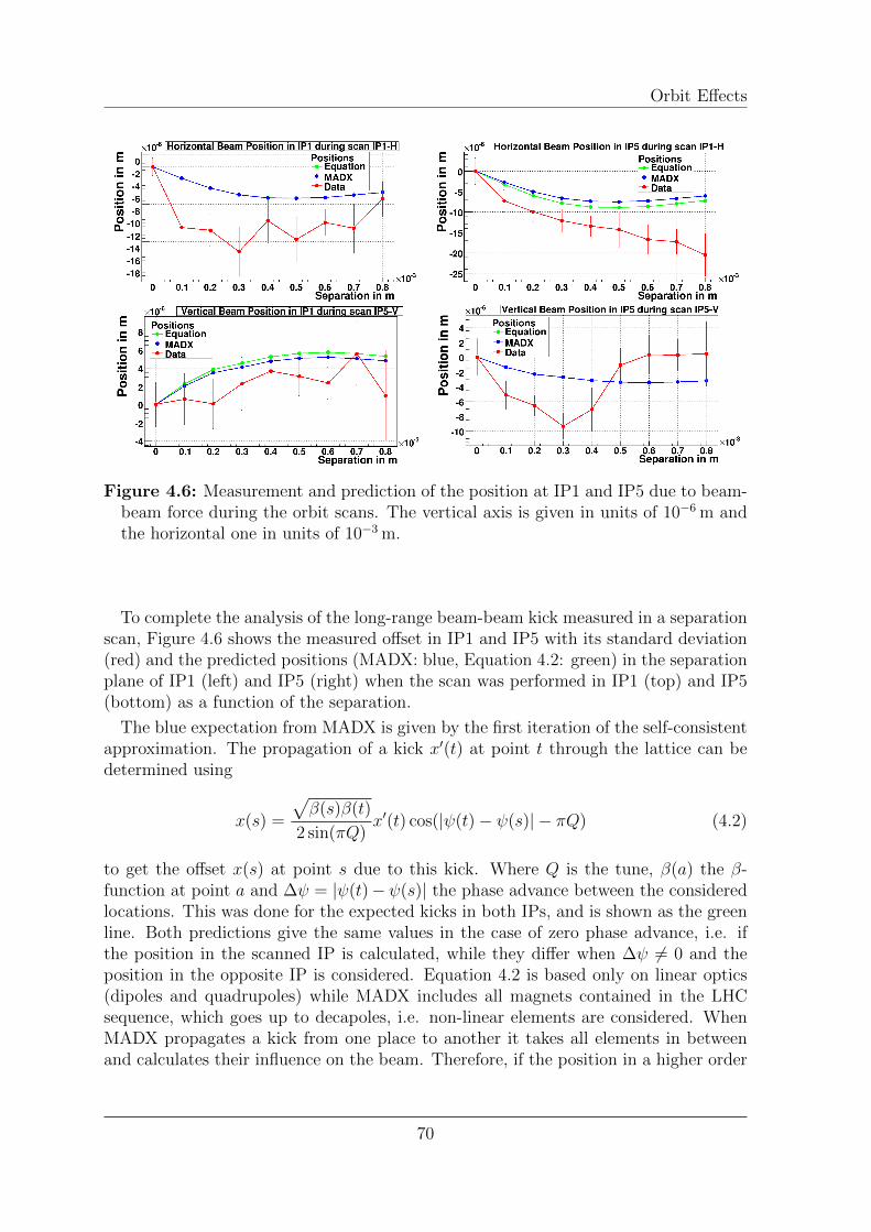
Orbit Effects
Figure 4.6: Measurement and prediction of the position at IP1 and IP5 due to beam-beam force during the orbit scans. The vertical axis is given in units of 10−6 m andthe horizontal one in units of 10−3 m.
To complete the analysis of the long-range beam-beam kick measured in a separationscan, Figure 4.6 shows the measured offset in IP1 and IP5 with its standard deviation(red) and the predicted positions (MADX: blue, Equation 4.2: green) in the separationplane of IP1 (left) and IP5 (right) when the scan was performed in IP1 (top) and IP5(bottom) as a function of the separation.
The blue expectation from MADX is given by the first iteration of the self-consistentapproximation. The propagation of a kick x′(t) at point t through the lattice can bedetermined using
x(s) =
√β(s)β(t)
2 sin(πQ)x′(t) cos(|ψ(t)− ψ(s)| − πQ) (4.2)
to get the offset x(s) at point s due to this kick. Where Q is the tune, β(a) the β-function at point a and ∆ψ = |ψ(t)−ψ(s)| the phase advance between the consideredlocations. This was done for the expected kicks in both IPs, and is shown as the greenline. Both predictions give the same values in the case of zero phase advance, i.e. ifthe position in the scanned IP is calculated, while they differ when ∆ψ 6= 0 and theposition in the opposite IP is considered. Equation 4.2 is based only on linear optics(dipoles and quadrupoles) while MADX includes all magnets contained in the LHCsequence, which goes up to decapoles, i.e. non-linear elements are considered. WhenMADX propagates a kick from one place to another it takes all elements in betweenand calculates their influence on the beam. Therefore, if the position in a higher order
70
Orbit Effects
element is non zero, non-linearities are introduced to the orbit which is not consideredin the equation, modifying the result.
Also here a discrepancy between prediction and measurement is found. Nevertheless,the position at the IPs were interpolated from the data of the two closest BPMs on theleft and right hand side of the IP only. Those BPMs are strip line BPMs and have aresolution of around ±5µm (see Chapter 4.2.2), which is not taken into account, but isalready larger than the standard deviation and the observed discrepancy. As expected,the shape of the curves agree with the prediction (except for the beam position in IP5during the scan of IP5, which needs further investigation). However, the source of thegap will be explained, when the gap in Figure 4.3 is understood.
4.2 Orbit Effects due to Bunch-by-Bunch
Differences
The beam-beam kicks from the parasitic interactions distort the orbits of the individ-ual bunches, due to the coherent dipolar component of the kick. Since the collisionpattern is different for different bunches, the orbits of all bunches are slightly different(PACMAN-effect, see Chapter 1.4). As a consequence, the orbits at the interactionpoints are different and the bunches collide with small offsets.
In the following observations of the bunch-by-bunch differences for the orbit positionin IP1 (ATLAS) will be presented, using different measurement methods to be able toaddress the effect in the two planes. Simulations were done in a previous study [6],which will be used to understand the observations.
4.2.1 Simulations
Figure 4.7 and 4.8 show simulations [6] of the offsets at the interaction point of ATLASin the vertical-crossing plane and in the horizontal-separation plane, respectively. ForCMS the same structure appears, but in inverted planes, since the the beams crosshorizontally. The top picture shows the positions for a perfect beam (all bunches areidentical) and the bottom one includes intensity variations between bunches of 20%.In daily operation the bunch-by-bunch intensity fluctuations are of the order of 10%to 20% [35], hence, 20% is a good approximation of the real conditions.
The simulations were done for the nominal filling scheme of LHC (see Figure 1.9)which exhibits a fourfold symmetry, therefore only one forth of the whole beam isshown. The red points represent beam 1 while the green ones show the positions ofbeam 2. Since the biggest contribution comes from IP1 and IP5, only those IPs weresimulated.
71
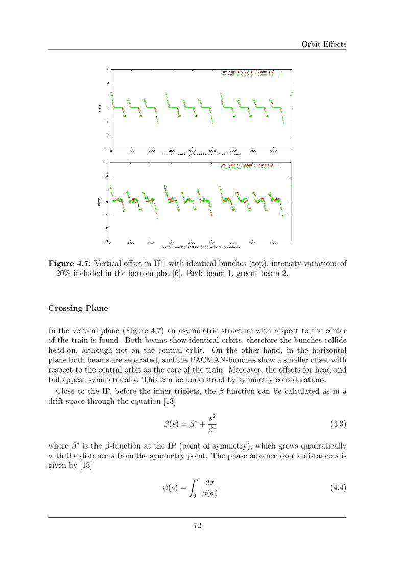
Orbit Effects
Figure 4.7: Vertical offset in IP1 with identical bunches (top), intensity variations of20% included in the bottom plot [6]. Red: beam 1, green: beam 2.
Crossing Plane
In the vertical plane (Figure 4.7) an asymmetric structure with respect to the centerof the train is found. Both beams show identical orbits, therefore the bunches collidehead-on, although not on the central orbit. On the other hand, in the horizontalplane both beams are separated, and the PACMAN-bunches show a smaller offset withrespect to the central orbit as the core of the train. Moreover, the offsets for head andtail appear symmetrically. This can be understood by symmetry considerations:
Close to the IP, before the inner triplets, the β-function can be calculated as in adrift space through the equation [13]
β(s) = β∗ +s2
β∗(4.3)
where β∗ is the β-function at the IP (point of symmetry), which grows quadraticallywith the distance s from the symmetry point. The phase advance over a distance s isgiven by [13]
ψ(s) =
∫ s
0
dσ
β(σ)(4.4)
72
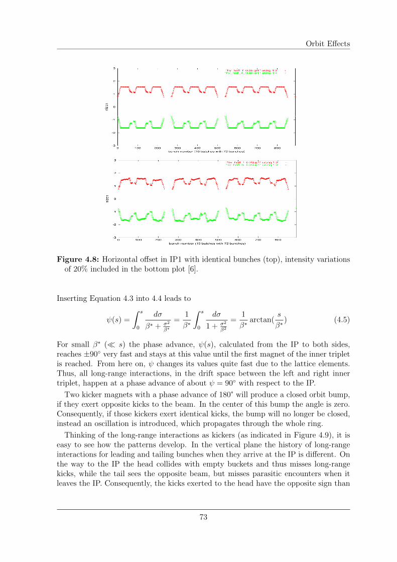
Orbit Effects
Figure 4.8: Horizontal offset in IP1 with identical bunches (top), intensity variationsof 20% included in the bottom plot [6].
Inserting Equation 4.3 into 4.4 leads to
ψ(s) =
∫ s
0
dσ
β∗ + σ2
β∗
=1
β∗
∫ s
0
dσ
1 + σ2
β2
=1
β∗arctan(
s
β∗) (4.5)
For small β∗ (� s) the phase advance, ψ(s), calculated from the IP to both sides,reaches ±90◦ very fast and stays at this value until the first magnet of the inner tripletis reached. From here on, ψ changes its values quite fast due to the lattice elements.Thus, all long-range interactions, in the drift space between the left and right innertriplet, happen at a phase advance of about ψ = 90◦ with respect to the IP.
Two kicker magnets with a phase advance of 180° will produce a closed orbit bump,if they exert opposite kicks to the beam. In the center of this bump the angle is zero.Consequently, if those kickers exert identical kicks, the bump will no longer be closed,instead an oscillation is introduced, which propagates through the whole ring.
Thinking of the long-range interactions as kickers (as indicated in Figure 4.9), it iseasy to see how the patterns develop. In the vertical plane the history of long-rangeinteractions for leading and tailing bunches when they arrive at the IP is different. Onthe way to the IP the head collides with empty buckets and thus misses long-rangekicks, while the tail sees the opposite beam, but misses parasitic encounters when itleaves the IP. Consequently, the kicks exerted to the head have the opposite sign than
73
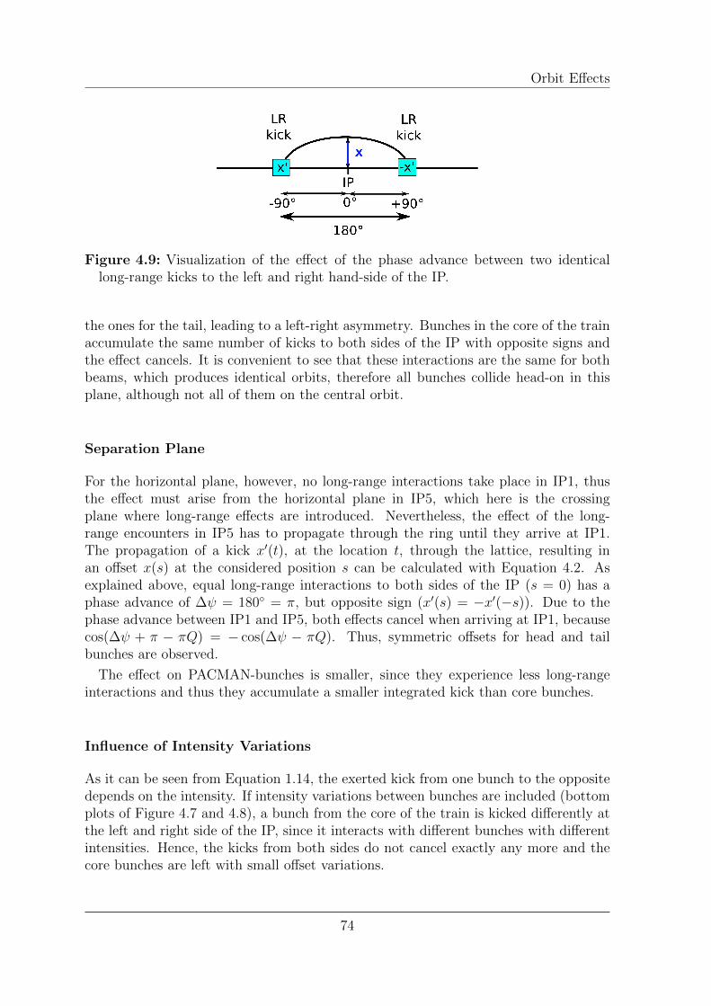
Orbit Effects
Figure 4.9: Visualization of the effect of the phase advance between two identicallong-range kicks to the left and right hand-side of the IP.
the ones for the tail, leading to a left-right asymmetry. Bunches in the core of the trainaccumulate the same number of kicks to both sides of the IP with opposite signs andthe effect cancels. It is convenient to see that these interactions are the same for bothbeams, which produces identical orbits, therefore all bunches collide head-on in thisplane, although not all of them on the central orbit.
Separation Plane
For the horizontal plane, however, no long-range interactions take place in IP1, thusthe effect must arise from the horizontal plane in IP5, which here is the crossingplane where long-range effects are introduced. Nevertheless, the effect of the long-range encounters in IP5 has to propagate through the ring until they arrive at IP1.The propagation of a kick x′(t), at the location t, through the lattice, resulting inan offset x(s) at the considered position s can be calculated with Equation 4.2. Asexplained above, equal long-range interactions to both sides of the IP (s = 0) has aphase advance of ∆ψ = 180◦ = π, but opposite sign (x′(s) = −x′(−s)). Due to thephase advance between IP1 and IP5, both effects cancel when arriving at IP1, becausecos(∆ψ + π − πQ) = − cos(∆ψ − πQ). Thus, symmetric offsets for head and tailbunches are observed.
The effect on PACMAN-bunches is smaller, since they experience less long-rangeinteractions and thus they accumulate a smaller integrated kick than core bunches.
Influence of Intensity Variations
As it can be seen from Equation 1.14, the exerted kick from one bunch to the oppositedepends on the intensity. If intensity variations between bunches are included (bottomplots of Figure 4.7 and 4.8), a bunch from the core of the train is kicked differently atthe left and right side of the IP, since it interacts with different bunches with differentintensities. Hence, the kicks from both sides do not cancel exactly any more and thecore bunches are left with small offset variations.
74
Orbit Effects
Details of the orbit effects
The unexpected bump feature for the first bunches of a batch, which is surrounded bybatches of the same train, is a combination of two effects: first those batches in themiddle of a train only have a distance of 8 missing bunches (225 ns) to the batch inthe front and back, therefore the first bunches will still see the tail of the leaving batchand the last bunches will interact already with the head of the next. Thus, the linearbehaviour as a function of the number of long-ranges, visible for PACMAN-bunchesbefore and after a larger gap (38 or 39 missing bunches) between trains is perturbed.Secondly, a gap of 8 bunches is enough to miss out long-range encounters in the driftspace, but not those in the triplet. Therefore, the last and first 8 bunches will have thesame number of long-range interactions but at different positions in the triplet magnetswhere the strength of the interaction differs.
For large amplitudes (r > 2σ) the strength of the long-range kick decreases with theseparation. But since Equation 1.14 is depending on the separation and the beam size,one has to take into account that the beam size changes with the β-function. In thedrift space around the IP, between the left and right inner triplet, the β-function canbe calculated with Equation 4.3. Hence, the beam size σ =
√βε ∝ s is approximately
proportional to the distance from the IP, for small β∗. Consequently, all long-rangeinteractions between the inner triplets to both sides of the IP can be approximated tohave the same strength, since the separation due to the crossing angle increases linearlyin this region, as well. Nevertheless, a closer investigation of Figure 4.1 shows that thislinearity with s stops at the first magnet next to the IP. From here, it is not straightforward to see which is the strongest long-range interaction, since separation and beamsize change differently due to the lattice properties.
4.2.2 Beam Position Monitors
The LHC Beam Position Monitors (BPM) have an acquisition mode that allows toacquire the orbit data bunch-by-bunch using an average over 225 turns to cancel the50 Hz noise. An exhaustive analysis of these data during a typical luminosity run hasbeen performed in order to assess the feasibility of those instruments to measure closedorbit deviations of the order of few micrometers, as they are expected from beam-beaminteractions. In the following the observations are summarized:
• The BPM noise on a bunch-by-bunch basis is consistent with what can be ex-pected from the current filtering algorithm applied to the data, and scales asexpected with BPM aperture: BPMSY (±7µm) > BPMSW (±5µm) > BPM(±3µm). The first two BPMs are strip line monitors and the last one is a buttonpick up. The left plot in Figure 4.10 shows an example of the residual noise fora button BPM.
• Most of the BPMs show pretty stable bunch-by-bunch orbits for a given orbit,even though the electronics reacts differently to different bunches in the train. Insome cases, however, e.g. BPM16L4 (Figure 4.10, right) some structure is still
75

Orbit Effects
visible (at the 10µm level) which probably still comes from the electronics.
• The difference between the mean position over several measurements before andafter the beams are brought into collisions gives, for some BPMs, offsets of theorder of 100 µm. A possible explanation could be that at the end of the squeezecertain orbit corrections are incorporated into the collision process in order toguarantee the reproducibility from fill to fill, and these orbit corrections could bethe source of the offset. Temperature effects cannot explain those offsets sincethey are of the order of few micrometers.
• Another systematic behaviour of the bunch-by-bunch data is that when the po-sition before and after collision are very similar, the result of the subtraction ofboth orbits becomes fairly flat (Figure 4.11, top). However, when the positionsare significantly different bunch-by-bunch structure becomes visible (Figure 4.11,bottom). A possible explanation could be the existence of a non-linearity in thebunch-by-bunch response of the electronics which depends upon the position.
The conclusion from the observations is that the LHC BPM system has a bunch-by-bunch orbit measurement which can give a relative bunch-to-bunch resolution inthe 5µm range. However, the non-linearity in the bunch-by-bunch measurement fordifferent global positions limits this resolution to ±50µm when comparing along thetrain for different mean positions. The current LHC BPM system therefore does nothave sufficient linearity or resolution to resolve the bunch-by-bunch orbit variations atthe few micrometer level expected from beam-beam interaction orbit effects.
# Bunch1000 1100 1200 1300 1400 1500
mµB
PM
po
siti
on
in
-8
-6
-4
-2
0
2
4
6
8
Orbit against Bunches for BPM.29L5.B1, Fill 1999c - B1 HorizontalOrbit against Bunches for BPM.29L5.B1, Fill 1999c - B1 Horizontal
# Bunch1000 1100 1200 1300 1400 1500
mµB
PM
po
siti
on
in
-10
0
10
20
30
Orbit against Bunches for BPM.16L4.B1, Fill 1999c - B1 HorizontalOrbit against Bunches for BPM.16L4.B1, Fill 1999c - B1 Horizontal
Figure 4.10: Example of the bunch-by-bunch signal before collisions after filtering forthe electronics effect. Left: a well behaving bottom BPM in the arc left to IP5, right:a bottom BPM with structures left in the arc to the left of IP4. A physics fill with1380 bunches spaced by 50 ns was analysed.
4.2.3 ATLAS Luminous Region Reconstruction
Ideally the position of the two beams should be measured separately. Unfortunately, theBPM system is the only device existing in the LHC able to measure the beam position
76
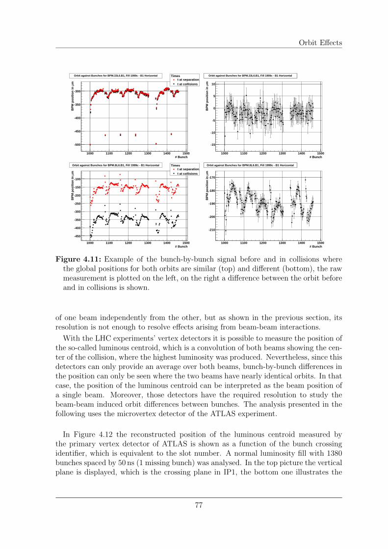
Orbit Effects
# Bunch1000 1100 1200 1300 1400 1500
mµB
PM
po
siti
on
in
-500
-450
-400
-350
-300
Orbit against Bunches for BPM.33L6.B1, Fill 1999c - B1 Horizontal Timest at separationt at collisions
# Bunch1000 1100 1200 1300 1400 1500
mµB
PM
po
siti
on
in
-15
-10
-5
0
5
10
Orbit against Bunches for BPM.33L6.B1, Fill 1999c - B1 HorizontalOrbit against Bunches for BPM.33L6.B1, Fill 1999c - B1 Horizontal
# Bunch1000 1100 1200 1300 1400 1500
mµB
PM
po
siti
on
in
-450
-400
-350
-300
-250
-200
-150
-100
Orbit against Bunches for BPM.8L6.B1, Fill 1999c - B1 Horizontal Timest at separationt at collisions
# Bunch1000 1100 1200 1300 1400 1500
mµB
PM
po
siti
on
in
-210
-200
-190
-180
-170
Orbit against Bunches for BPM.8L6.B1, Fill 1999c - B1 HorizontalOrbit against Bunches for BPM.8L6.B1, Fill 1999c - B1 Horizontal
Figure 4.11: Example of the bunch-by-bunch signal before and in collisions wherethe global positions for both orbits are similar (top) and different (bottom), the rawmeasurement is plotted on the left, on the right a difference between the orbit beforeand in collisions is shown.
of one beam independently from the other, but as shown in the previous section, itsresolution is not enough to resolve effects arising from beam-beam interactions.
With the LHC experiments’ vertex detectors it is possible to measure the position ofthe so-called luminous centroid, which is a convolution of both beams showing the cen-ter of the collision, where the highest luminosity was produced. Nevertheless, since thisdetectors can only provide an average over both beams, bunch-by-bunch differences inthe position can only be seen where the two beams have nearly identical orbits. In thatcase, the position of the luminous centroid can be interpreted as the beam position ofa single beam. Moreover, those detectors have the required resolution to study thebeam-beam induced orbit differences between bunches. The analysis presented in thefollowing uses the microvertex detector of the ATLAS experiment.
In Figure 4.12 the reconstructed position of the luminous centroid measured bythe primary vertex detector of ATLAS is shown as a function of the bunch crossingidentifier, which is equivalent to the slot number. A normal luminosity fill with 1380bunches spaced by 50 ns (1 missing bunch) was analysed. In the top picture the verticalplane is displayed, which is the crossing plane in IP1, the bottom one illustrates the
77
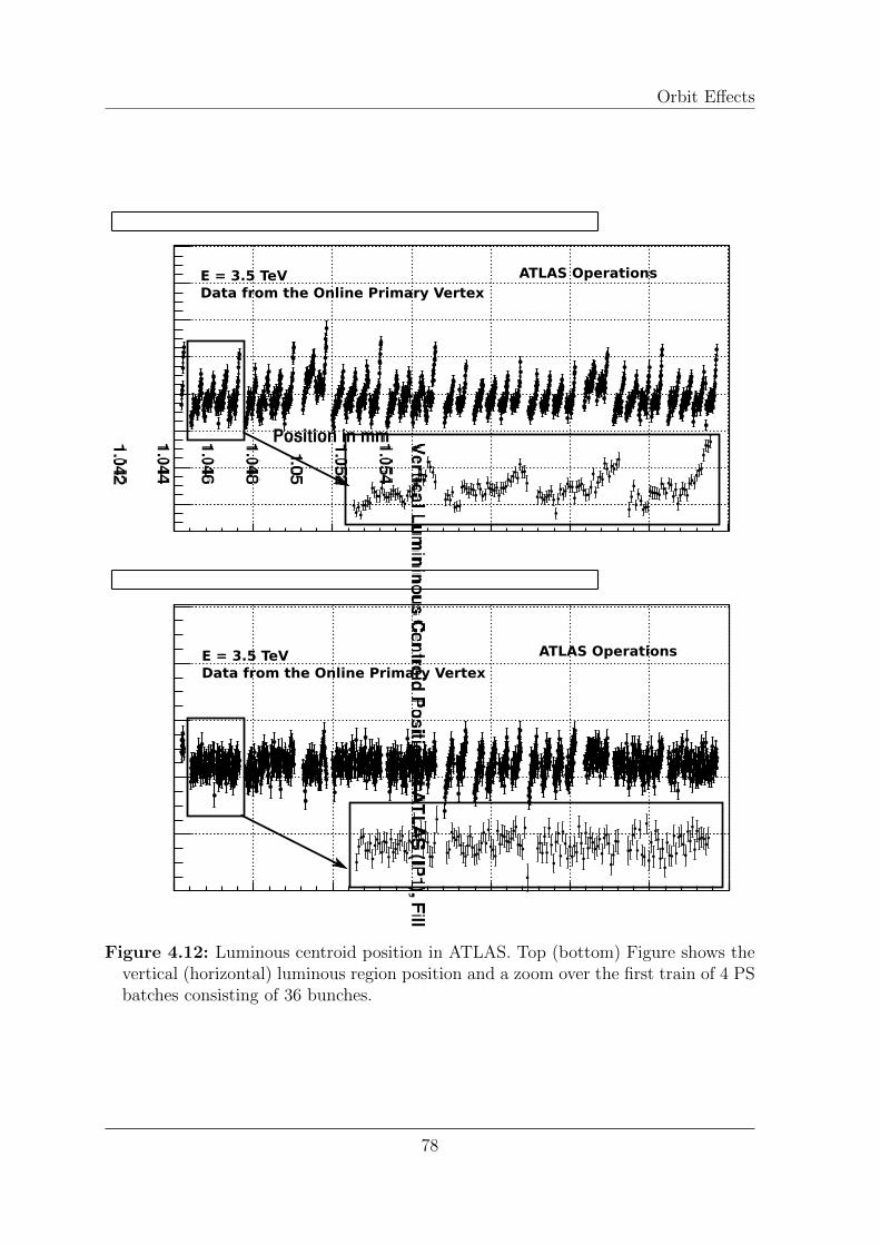
Orbit Effects
ATLAS OperationsE = 3.5 TeVData from the Online Primary Vertex
E = 3.5 TeVData from the Online Primary Vertex
ATLAS Operations
Figure 4.12: Luminous centroid position in ATLAS. Top (bottom) Figure shows thevertical (horizontal) luminous region position and a zoom over the first train of 4 PSbatches consisting of 36 bunches.
78
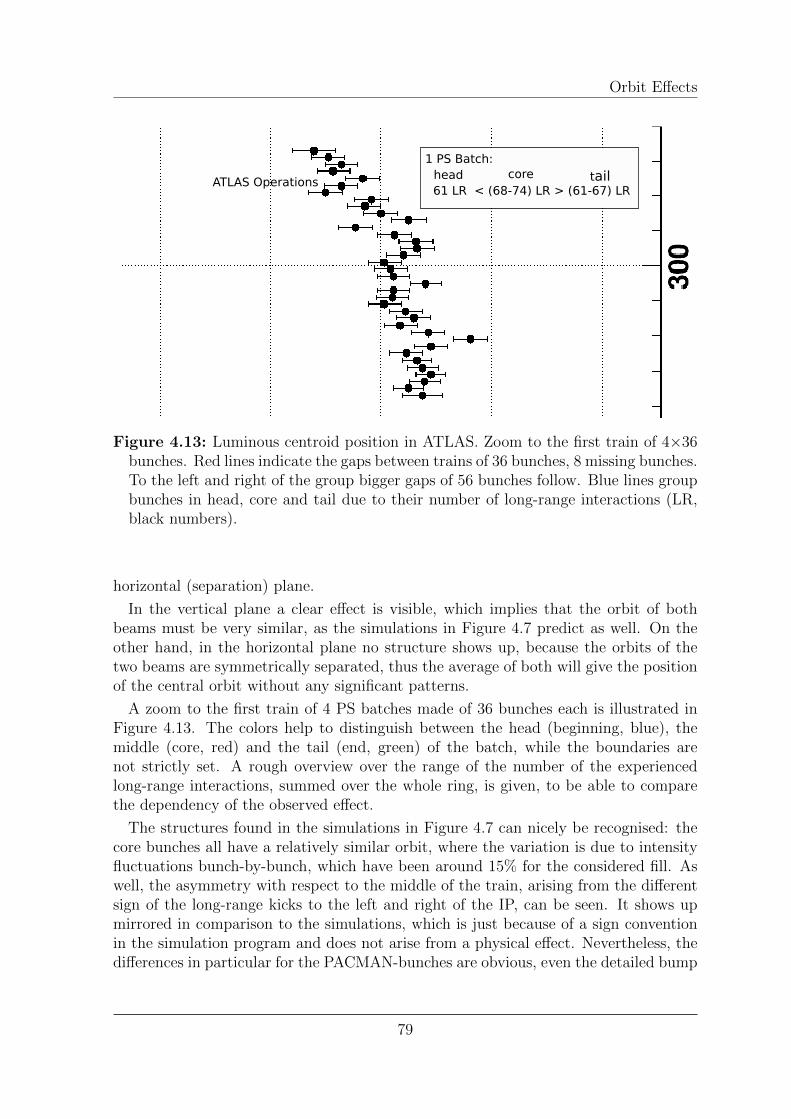
Orbit Effects
1 PS Batch:head core tail61 LR < (68-74) LR > (61-67) LR
ATLAS Operations
Figure 4.13: Luminous centroid position in ATLAS. Zoom to the first train of 4×36bunches. Red lines indicate the gaps between trains of 36 bunches, 8 missing bunches.To the left and right of the group bigger gaps of 56 bunches follow. Blue lines groupbunches in head, core and tail due to their number of long-range interactions (LR,black numbers).
horizontal (separation) plane.
In the vertical plane a clear effect is visible, which implies that the orbit of bothbeams must be very similar, as the simulations in Figure 4.7 predict as well. On theother hand, in the horizontal plane no structure shows up, because the orbits of thetwo beams are symmetrically separated, thus the average of both will give the positionof the central orbit without any significant patterns.
A zoom to the first train of 4 PS batches made of 36 bunches each is illustrated inFigure 4.13. The colors help to distinguish between the head (beginning, blue), themiddle (core, red) and the tail (end, green) of the batch, while the boundaries arenot strictly set. A rough overview over the range of the number of the experiencedlong-range interactions, summed over the whole ring, is given, to be able to comparethe dependency of the observed effect.
The structures found in the simulations in Figure 4.7 can nicely be recognised: thecore bunches all have a relatively similar orbit, where the variation is due to intensityfluctuations bunch-by-bunch, which have been around 15% for the considered fill. Aswell, the asymmetry with respect to the middle of the train, arising from the differentsign of the long-range kicks to the left and right of the IP, can be seen. It shows upmirrored in comparison to the simulations, which is just because of a sign conventionin the simulation program and does not arise from a physical effect. Nevertheless, thedifferences in particular for the PACMAN-bunches are obvious, even the detailed bump
79
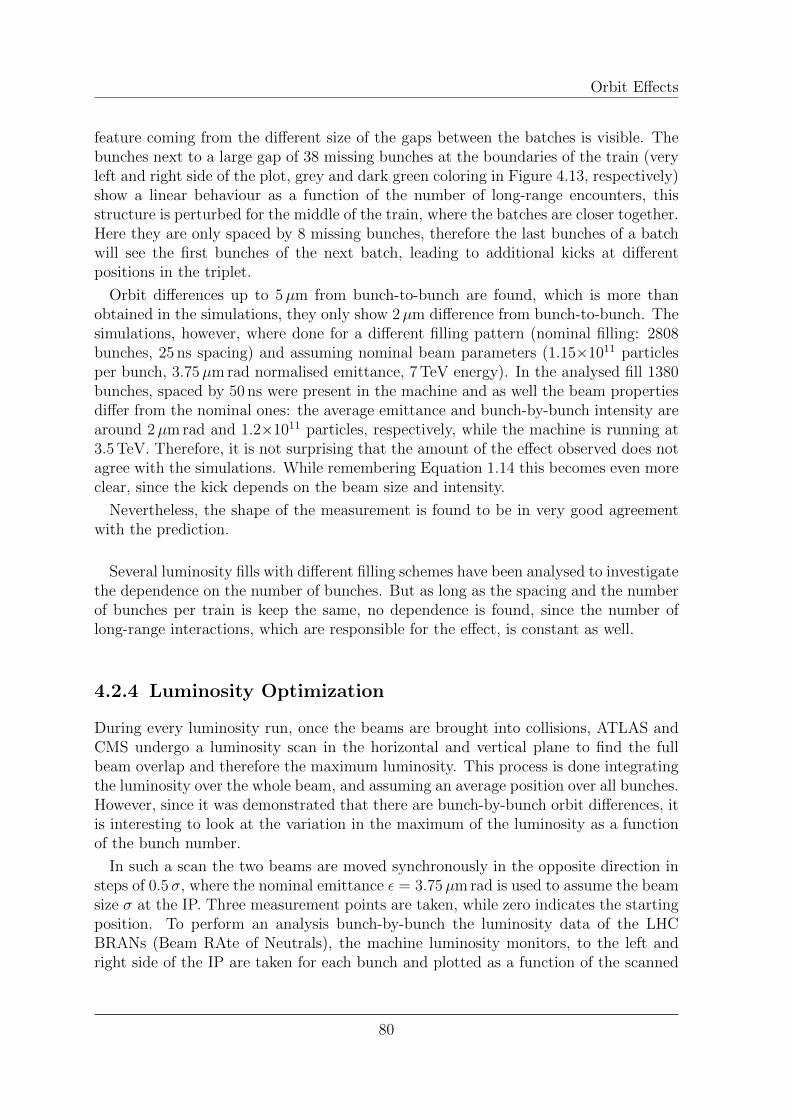
Orbit Effects
feature coming from the different size of the gaps between the batches is visible. Thebunches next to a large gap of 38 missing bunches at the boundaries of the train (veryleft and right side of the plot, grey and dark green coloring in Figure 4.13, respectively)show a linear behaviour as a function of the number of long-range encounters, thisstructure is perturbed for the middle of the train, where the batches are closer together.Here they are only spaced by 8 missing bunches, therefore the last bunches of a batchwill see the first bunches of the next batch, leading to additional kicks at differentpositions in the triplet.
Orbit differences up to 5µm from bunch-to-bunch are found, which is more thanobtained in the simulations, they only show 2µm difference from bunch-to-bunch. Thesimulations, however, where done for a different filling pattern (nominal filling: 2808bunches, 25 ns spacing) and assuming nominal beam parameters (1.15×10¹¹ particlesper bunch, 3.75µm rad normalised emittance, 7 TeV energy). In the analysed fill 1380bunches, spaced by 50 ns were present in the machine and as well the beam propertiesdiffer from the nominal ones: the average emittance and bunch-by-bunch intensity arearound 2µm rad and 1.2×10¹¹ particles, respectively, while the machine is running at3.5 TeV. Therefore, it is not surprising that the amount of the effect observed does notagree with the simulations. While remembering Equation 1.14 this becomes even moreclear, since the kick depends on the beam size and intensity.
Nevertheless, the shape of the measurement is found to be in very good agreementwith the prediction.
Several luminosity fills with different filling schemes have been analysed to investigatethe dependence on the number of bunches. But as long as the spacing and the numberof bunches per train is keep the same, no dependence is found, since the number oflong-range interactions, which are responsible for the effect, is constant as well.
4.2.4 Luminosity Optimization
During every luminosity run, once the beams are brought into collisions, ATLAS andCMS undergo a luminosity scan in the horizontal and vertical plane to find the fullbeam overlap and therefore the maximum luminosity. This process is done integratingthe luminosity over the whole beam, and assuming an average position over all bunches.However, since it was demonstrated that there are bunch-by-bunch orbit differences, itis interesting to look at the variation in the maximum of the luminosity as a functionof the bunch number.
In such a scan the two beams are moved synchronously in the opposite direction insteps of 0.5σ, where the nominal emittance ε = 3.75µm rad is used to assume the beamsize σ at the IP. Three measurement points are taken, while zero indicates the startingposition. To perform an analysis bunch-by-bunch the luminosity data of the LHCBRANs (Beam RAte of Neutrals), the machine luminosity monitors, to the left andright side of the IP are taken for each bunch and plotted as a function of the scanned
80
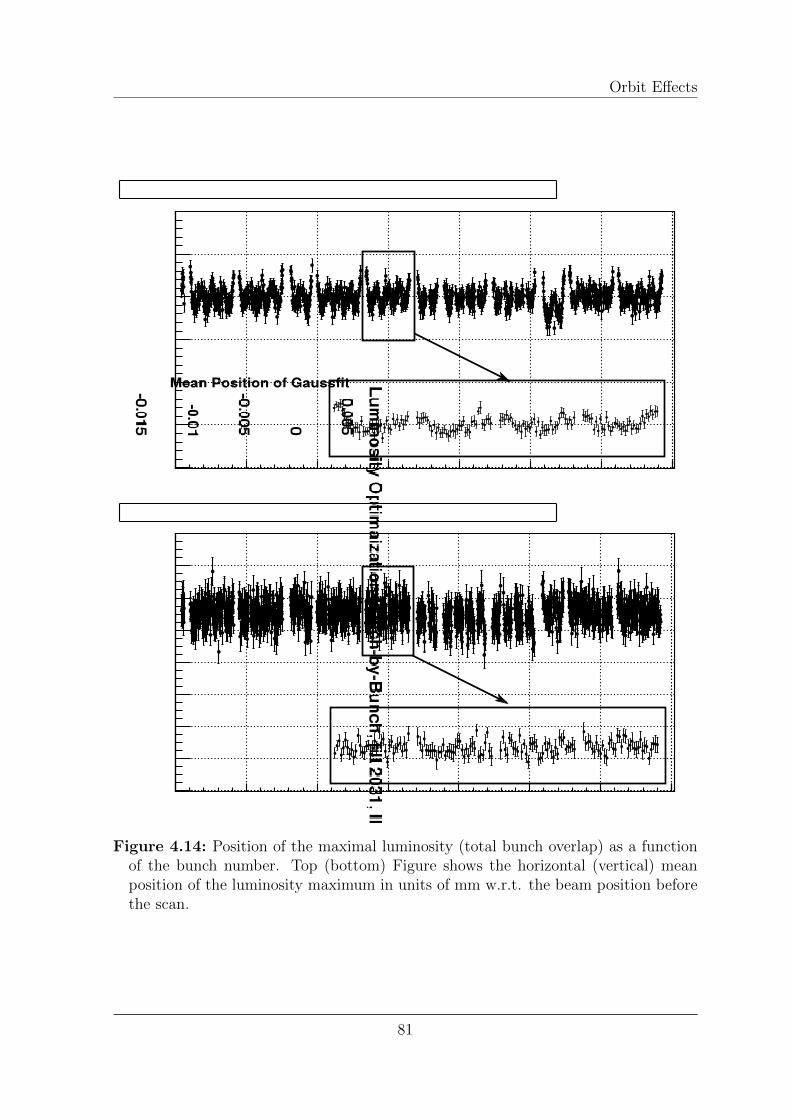
Orbit Effects
Figure 4.14: Position of the maximal luminosity (total bunch overlap) as a functionof the bunch number. Top (bottom) Figure shows the horizontal (vertical) meanposition of the luminosity maximum in units of mm w.r.t. the beam position beforethe scan.
81
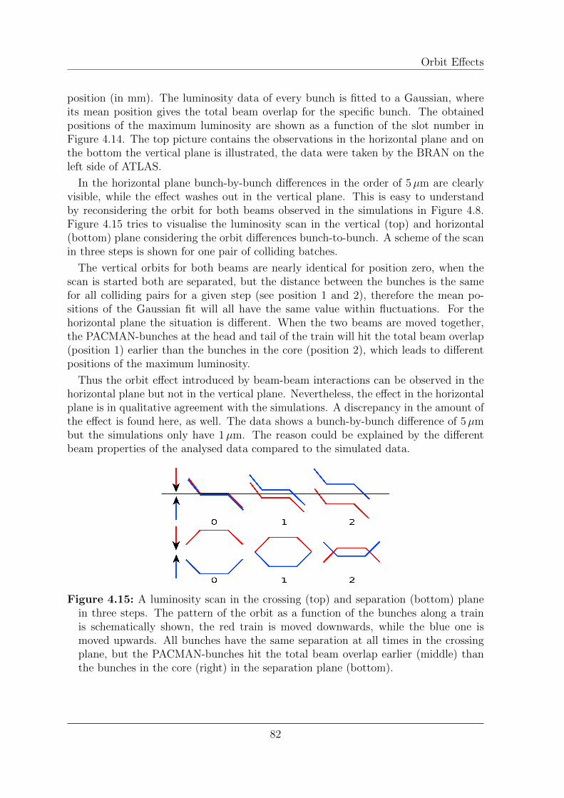
Orbit Effects
position (in mm). The luminosity data of every bunch is fitted to a Gaussian, whereits mean position gives the total beam overlap for the specific bunch. The obtainedpositions of the maximum luminosity are shown as a function of the slot number inFigure 4.14. The top picture contains the observations in the horizontal plane and onthe bottom the vertical plane is illustrated, the data were taken by the BRAN on theleft side of ATLAS.
In the horizontal plane bunch-by-bunch differences in the order of 5µm are clearlyvisible, while the effect washes out in the vertical plane. This is easy to understandby reconsidering the orbit for both beams observed in the simulations in Figure 4.8.Figure 4.15 tries to visualise the luminosity scan in the vertical (top) and horizontal(bottom) plane considering the orbit differences bunch-to-bunch. A scheme of the scanin three steps is shown for one pair of colliding batches.
The vertical orbits for both beams are nearly identical for position zero, when thescan is started both are separated, but the distance between the bunches is the samefor all colliding pairs for a given step (see position 1 and 2), therefore the mean po-sitions of the Gaussian fit will all have the same value within fluctuations. For thehorizontal plane the situation is different. When the two beams are moved together,the PACMAN-bunches at the head and tail of the train will hit the total beam overlap(position 1) earlier than the bunches in the core (position 2), which leads to differentpositions of the maximum luminosity.
Thus the orbit effect introduced by beam-beam interactions can be observed in thehorizontal plane but not in the vertical plane. Nevertheless, the effect in the horizontalplane is in qualitative agreement with the simulations. A discrepancy in the amount ofthe effect is found here, as well. The data shows a bunch-by-bunch difference of 5µmbut the simulations only have 1µm. The reason could be explained by the differentbeam properties of the analysed data compared to the simulated data.
Figure 4.15: A luminosity scan in the crossing (top) and separation (bottom) planein three steps. The pattern of the orbit as a function of the bunches along a trainis schematically shown, the red train is moved downwards, while the blue one ismoved upwards. All bunches have the same separation at all times in the crossingplane, but the PACMAN-bunches hit the total beam overlap earlier (middle) thanthe bunches in the core (right) in the separation plane (bottom).
82
Conclusion
5 Conclusion
Beam-beam observations at LHC are presented for the first time in this thesis. Datafrom dedicated machine study periods as well as data from normal luminosity runshave been analysed focusing on head-on or long-range interaction effects.
An important effect of the head-on interactions is the introduced tune shift. Indedicated experiments with a few bunches and by absence of long-range encounters themaximum coherent beam-beam parameter achievable was probed at injection energy.Linear tune shifts almost 5 times higher as the expected value under nominal conditionswere obtained without obvious emittance growth and lifetime problems. Whereas,bunch intensities as high as 2×10¹¹ protons and small emittances of 1.2µm rad werereached.
Unfortunately, this could only be calculated from the measured beam sizes andintensities. A direct tune measurement was not available. Due to the transverse damperthe BBQ data was unusable at the important moment the beams were brought intocollisions. Moreover, the Schottky monitors are still under commissioning and were aswell not able to provide adequate data.
Nevertheless, the stability of the beam at the achieved high brightnesses and thecalculations show the success of the experiment: no head-on beam-beam limits couldbe found yet. The experiment will be repeated at top energy (3.5 TeV) in one of thenext machine development periods to probe the operational conditions of the machineand investigate if this has any influence on the results.
Orbit effects due to beam-beam interactions could clearly be measured. In a ded-icated experiment it was possible to measure the long-range beam-beam kick withsingle colliding bunches during a separation scan. The shape of this measurementnicely follows the expectation, though, a small gap between the data and the predic-tion is present, which could not be explained yet. Further investigations and a secondmeasurement are necessary to understand the discrepancy. However, this was the firsttime such a study was done at LHC and the agreement is already good.
Coming from optimized and dedicated experiments, where the theory is tested, to realoperational conditions, the expected bunch-by-bunch differences due to the differentcollision patterns between bunches are seen. The long-range effect was demonstratedin both planes of IP1 with the aid of two different measurement methods (luminousregion reconstruction and luminosity scan), since each method is only able to resolve
83
Conclusion
one plane. The LHC BPM system, as it measures the two beams separately in eachplane, could not be used for the analysis, because the effects are to small to be resolvedby the devices.
The differences for the so-called PACMAN-bunches were investigated and they are inqualitative agreement with the simulations performed for the nominal injection scheme.Since the analysed data was taken at 3.5 TeV, with a bunch spacing of 50 ns and non-nominal beam parameters they do not fully agree quantitatively. New simulations areforeseen with the actual filling pattern and parameters to confirm the amount of theeffect, as well. Moreover, the analysis must be repeated for IP5 to verify the samebehaviour, as expected.
All in all, it can be concluded from the observations that perturbations of the beamsfrom beam-beam interactions are clearly present and observable, but machine operationin the presence of them is still possible and no limits could be found yet. Therefore,beam-beam effects should allow to operate at nominal luminosity at 7 TeV.
84
Acknowledgement
6 Acknowledgement
This thesis would not have been possible without the guidance and the help of severalindividuals who in one way or another contributed and extended their valuable assis-tance in the preparation and completion of this study.
First I would like to express my gratitude to my thesis advisor Prof. Dr. Achim Stahl,for the possibility of writing this thesis. I am thankful for the revealing discussions andfor the freedom he gave me during the whole process of preparing this work.
I am heartily thankful to my supervisor, Dr. Reyes Alemany Fernandez, whoseencouragement, supervision and support from the preliminary to the concluding levelenabled me to develop an understanding of the subject.
It is a pleasure to thank Dr. Bernhard Holzer for his support in the decision of thetopic and especially for the many coffee talks we had to solve problems of all kind, theywere always very interesting and helpful.
I would like to thank the LHC Operations Group and the Beam-Beam WorkingGroup for their support during the machine development studies. Moreover, I amindebted to Dr. Werner Herr, Dr. Tatiana Pieloni, Dr. Jorg Wenniger, Dr. MathildeFavier, Dr. Rhodri Jones, Dr. Eva Calvo, Dipl.-Phys. Tobias Bar and Dipl.-Phys.Gabriel Muller for their fruitful discussions during the analysis of the data.
I would also like to acknowledge the ATLAS Collaboration for providing the beamspot information from their data. In particular I am grateful to Dr. Rainer Bartoldus,Dr. Josh Cogan, Dr. Carl Gwilliam, Dr. Emanuel Strauss and Dr. Christoph Rembserfor their help.
Many thanks to all of you, it was a nice time and a great experience to work withyou.
85

Bibliography
Bibliography
[1] W. Herr, Beam-Beam Effects, Cockcroft Institute Lectures (2009),http://zwe.home.cern.ch/zwe/talks/cockcroft beambeam.pdf.
[2] W. Herr, Beam-Beam Interactions, CAS - CERN Accelerator School: Interme-diate Course on Accelerator Physics, Zeuthen, Germany (2003).
[3] T. Pieloni, A Study of Beam-Beam Effects in Hadron Colliders with a LargeNumber of Bunches, These no 4211 (2008).
[4] W. Herr and B. Muratori, Concept of luminosity, CAS - CERN AcceleratorSchool: Intermediate Course on Accelerator Physics, Zeuthen, Germany, pp.361-378, (2003).
[5] J. D. Jackson, Classical Electrodynamics, John Wiley & Sons, ISBN 978-0471309321.
[6] W. Herr, Features and implications of different LHC crossing schemes, LHCProject Report 628, Geneva, Switzerland, 2003
[7] R. Bailey, P. Collier, Standard Filling Schemes for Various LHC OperationModes (Revised), LHC-Project Note 323 Revised (2003).
[8] LHC Design Report Volume I - The LHC main ring, CERN, Geneva, CERN-2004-003-V-1.
[9] LHC Design Report Volume II - The LHC Infrastructure and General Services,CERN, Geneva, CERN-2004-003-V-2.
[10] LHC Design Report Volume III - The LHC Injector Chain, CERN, Geneva,CERN-2004-003-V-3.
[11] CERN faq - LHC the guide, CERN-Brochure-2009-003-Eng.
[12] www.cern.ch.
[13] K. Wille, The Physics of Particle Accelerators - an introduction Oxford Univer-sity Press, ISBN 0-19-850549-3.
[14] http://www.americanmagnetics.com/charactr.php.
[15] P. Forck, Lecture Notes on Beam Instrumenteation and Diagnostics, JUAS 2011,www-bd.gsi.de/conf/juas/juas.html.
[16] D. Cocq, The wide band normaliser - a new circuit to measure transverse bunchposition in accelerators and colliders, Nuclear Instruments and Methods inPhysics Research A 416 (1998) p.1-8.
[17] O.R. Jones, Commissioning and First Performance of the LHC Beam Instru-mentation, CERN, Geneva, Switzerland (2010), CERN-BE-2010-007 BI.
87
Bibliography
[18] E. Calvo et al., The LHC Orbit and Trajectory System, Proceedings DIPAC2003, Mainz, Germany, CERN-AB-2003-057 BDI.
[19] Particle Data Group, Particle Data Booklet, http://pdg.lbl.gov/, 2010.
[20] Ch. Steinbach, Wire Scanner, Collaboration website for the edition ofthe report on 50 years of the Proton Synchrotron, https://project-ps50.web.cern.ch/project-PS50/.
[21] CAS - CERN Accelerator School, Beam Diagnostics, Dourdan, France (2008),CERN-2009-005.
[22] R. Jung, P. Komorowski, L. Ponce, D. Tommasini, The LHC 450 GeV to 7TeV Synchrotron Radiation Profile Monitor using a Superconducting Undulator,CERN-SL-2002-015 BI.
[23] A. S. Fisher et al., First Beam Measurements with the LHC Synchrotron LightMonitor, CERN-BE-2010-019 BI.
[24] A. Jeff et al., Spatial and Temporal Beam Profiles for the LHC using SynchrotronLight, Proc. of SPIE Vol. 7726, 77261J.
[25] F. Roncarolo, Can we get a reliable on-line measurement of the transverse beamsize?, LHC Evian Workshop (2010).
[26] L. Ponce, R. Jung and F. Meot, LHC Proton Beam Diagnostics using Syn-chrotron Radiation, CERN-2004-007.
[27] http://emetral.web.cern.ch/emetral/ICEsection/2011-02-09/Presentation1.pdf.
[28] F. Caspers et al., The 4.8 GHz LHC Schottky Pick-Up System, Proceedings ofPAC07, Albuquerque, New Mexico, USA, FRPMN068.
[29] http://ab-dep-bi-pm.web.cern.ch/ab-dep-bi-pm/?n=Activities.BRAN.
[30] R. Alemany, M. Lamont, S. M. White, Separation Scan Application Require-ments, LHC Project Document, Geneva, Switzerland (2008), LHC-OP-ES-0010.
[31] W. Herr et al., Head-On beam-beam tune shift with high brightness beams in theLHC, CERN-ATS-Note-2011-029 MD, 2011.
[32] W. Herr et al., Head-on beam-beam collisions with high intensities and long rangebeam-beam studies in the LHC, CERN-ATS-Note-2011-058 MD, 2011.
[33] A. S. Fisher, Expected Performance of the LHC Synchrotron-Light Telescope(BSRT) and Abort-Gap Monitor (BSRA), LHC Performance Note-014, 2009.
[34] http://wwwslap.cern.ch/mad/.
[35] R. Garoby, Multiple splitting in the PS: results and alternative filling schemes,Proc. LHC workshop, CHARMONIX XI, Charmonix 2001, CERN-SL-2001-003(DI).
88