Embed Size (px)
Citation preview

Beacon Buster EE382: Intro to Design Final Paper
Anthony Baca
Joseph S. Gabaldon
Joseph Kloeppel
Garrett Newell
May 6, 2014

1 | P a g e
Table of Contents 1. List of Figures ........................................................................................................................................ 2
2. Abstract ................................................................................................................................................. 3
3. Introduction .......................................................................................................................................... 3
4. Requirements ........................................................................................................................................ 4
5. Subsystems ........................................................................................................................................... 4
5.1. Locomotion and Chassis System ................................................................................................... 5
5.2. Power System ............................................................................................................................... 8
5.3. RF Front End System ................................................................................................................... 11
5.4. Control and Data Handling System ............................................................................................. 17
5.5. Post-Processing System .............................................................................................................. 22
6. Budget ................................................................................................................................................. 26
7. Timeline ............................................................................................................................................... 26
8. Testing ................................................................................................................................................. 26
9. Final Results ........................................................................................................................................ 27
10. Conclusion ....................................................................................................................................... 28
11. Appendices ...................................................................................................................................... 29
Appendix A: Final Code for Robot ........................................................................................................... 29
Appendix B: MATLAB Codes.................................................................................................................... 40
Triangulation: ...................................................................................................................................... 40
Demodulation: .................................................................................................................................... 42
Appendix C: Visual Basic Codes ............................................................................................................... 44
Appendix D: Power Budget ..................................................................................................................... 53
12. References ...................................................................................................................................... 53
DataSheets: ............................................................................................................................................. 53
Code examples: ....................................................................................................................................... 54

2 | P a g e
1. List of Figures Figure 1: DIK Pyramid .................................................................................................................................... 3
Figure 2: Subsystem Block Diagram .............................................................................................................. 5
Figure 3: Motors and Frame ......................................................................................................................... 5
Figure 4: Custom Chassis .............................................................................................................................. 6
Figure 5: Custom Chassis Cuts and Folds ...................................................................................................... 6
Figure 6: Custom Antenna Mount ................................................................................................................ 6
Figure 7: Final Chassis and Locomotion Build ............................................................................................... 7
Figure 8: Power System Block Diagram ........................................................................................................ 8
Figure 9: Motor Controller Block Diagram .................................................................................................... 9
Figure 10: Logic Level Shifter ........................................................................................................................ 9
Figure 11: 5V Power Regulator Circuit ........................................................................................................ 10
Figure 12: 3.3V Power Regulator Circuit ..................................................................................................... 10
Figure 13: Proto Board of RF Amplifiers Regulators ................................................................................... 11
Figure 14: RF Front End System Block Diagram .......................................................................................... 12
Figure 15: Angular Power Received Plot ..................................................................................................... 13
Figure 16: Output of Mixer and Band Pass Filter on Spectrum Analyzer ................................................... 14
Figure 17: AD8307 Log Amp Circuit ............................................................................................................ 15
Figure 18: Super Diode Peak Detector with Drain ...................................................................................... 16
Figure 19: Schmitt Trigger ........................................................................................................................... 16
Figure 20: Output of RF Front End System ................................................................................................. 17
Figure 21: Arduino Due ............................................................................................................................... 18
Figure 22: GPS Module................................................................................................................................ 19
Figure 23: Peak Detector Sweep with Moving Average Filter .................................................................... 20
Figure 24: Location Stops ............................................................................................................................ 21
Figure 25: Triangulation Method ................................................................................................................ 23
Figure 26: Custom Graphical User Interface ............................................................................................... 24
Figure 27: GUI with Recorded Data ............................................................................................................ 25
Table 1: Budget ........................................................................................................................................... 26
Table 2: Timeline ......................................................................................................................................... 26
3 | P a g e
2. Abstract In electronics, locating beacons can be an important tool for various situations. The Beacon Buster
takes the task of finding the GPS coordinates of a beacon emitting a signal to new heights, with state-of-
the-art software and tailor made hardware, all while decoding a Frequency Shift Key signal being
emitted by the beacon. The following information will explain how the Beacon Buster works, as well as
why many of the decisions made in the design were chosen. The various subsystems will also be
explained in detail, and an overview of the final product will be given.
3. Introduction As technology becomes increasingly widespread, the ease in which engineers and technologists
collect data also improves; electrical devices, with their various sensors and data acquisition
components, are becoming more and more important in daily life. With the advent of “The Internet of
Things,” as technology moves from the abstract to the physical, this trend will only increase.
The challenge currently facing the industry is not collecting more data, but collecting useful data
and correctly utilizing it. Robust systems must be designed that can not only acquire all relevant data,
but also correctly interpolate that data into information, and finally supply the technology's users with
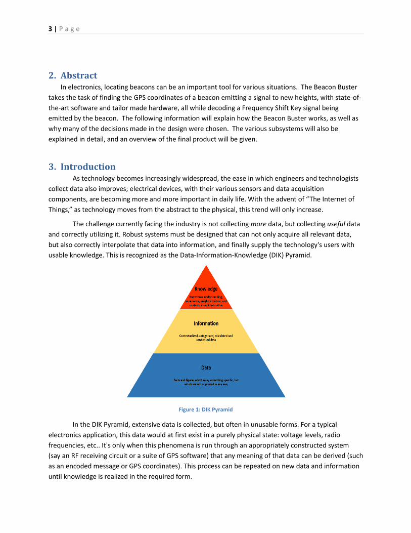
usable knowledge. This is recognized as the Data-Information-Knowledge (DIK) Pyramid.
Figure 1: DIK Pyramid
In the DIK Pyramid, extensive data is collected, but often in unusable forms. For a typical
electronics application, this data would at first exist in a purely physical state: voltage levels, radio
frequencies, etc.. It's only when this phenomena is run through an appropriately constructed system
(say an RF receiving circuit or a suite of GPS software) that any meaning of that data can be derived (such
as an encoded message or GPS coordinates). This process can be repeated on new data and information
until knowledge is realized in the required form.

4 | P a g e
By dealing with data in a systematic nature, we can produce any requested knowledge. This
paper lays out the design of one such system.
4. Requirements To design a robot that located the GPS coordinates of a radio beacon emitting a Frequency
Shifted Key (FSK) signal with a baud rate of 600 and alternating frequencies of 2.15GHz and 2.20GHz.
Once located, the robot must decode the signal. Everything must be done autonomously (aside from
Post-Processing). Robot must also meet the following conditions:
Built with a collection of supplied RF components and motors
Extra budget of $325
Completed within duration of the class (1/18 – 5/1)
Containing a custom part
There were some other notable constraints that had to be accounted for:
Robot had to operate in an environment with a tested noise floor of -70dBm
Robot had to deal with reflections off nearby buildings (3-4 stories)
Robot had to evade nearby concentrated WiFi frequency of 2.4GHz
Robot had to have a high degree of accuracy that would be under scrutiny
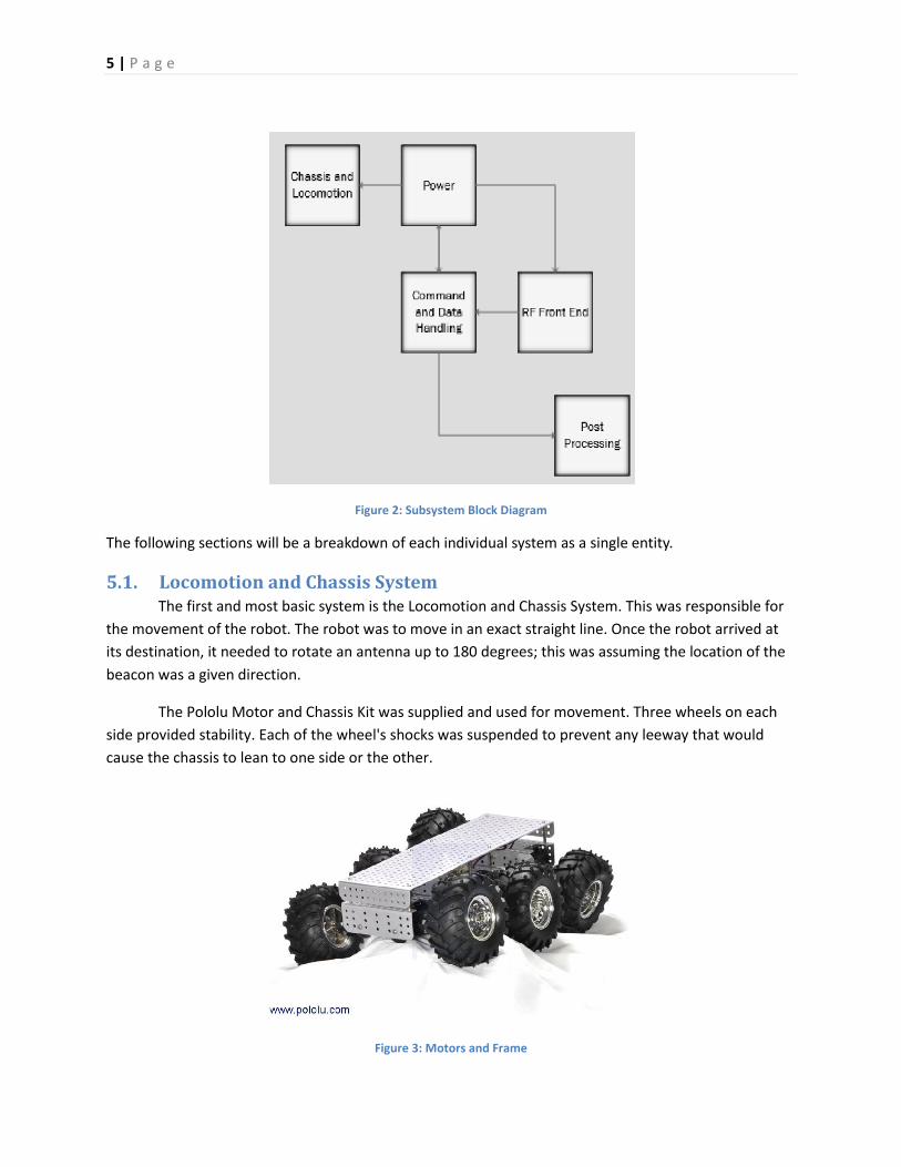
5. Subsystems The design of the robot consisted of 5 main subsystems. By dividing the robot in such a way, it
was possible to focus on each individual subsystem as a specific purpose with a set of outputs/inputs (a
desirable pattern of design). This made extensive use of unit testing and prototypes. Such a top-down
approach provided clarity, coordination, and concentration.
Robot consists of the following 5 subsystems (referred to as systems or subsystems, hereafter):
1. Locomotion and Chassis System
2. Power System
3. (Radio Frequency) RF Front End System
4. Control and Data Handling System
5. Post-Processing System
5 | P a g e
Figure 2: Subsystem Block Diagram
The following sections will be a breakdown of each individual system as a single entity.
5.1. Locomotion and Chassis System The first and most basic system is the Locomotion and Chassis System. This was responsible for
the movement of the robot. The robot was to move in an exact straight line. Once the robot arrived at
its destination, it needed to rotate an antenna up to 180 degrees; this was assuming the location of the
beacon was a given direction.
The Pololu Motor and Chassis Kit was supplied and used for movement. Three wheels on each
side provided stability. Each of the wheel's shocks was suspended to prevent any leeway that would
cause the chassis to lean to one side or the other.
Figure 3: Motors and Frame

6 | P a g e
An extra chassis was built in order to house more electronics. The extra chassis would also be
custom built to support a servo motor to turn the antenna; a hole was cut at the top to allow a rotating
platform to be mounted. This was constructed from a 22 gauge sheet of metal, carefully folded. The
chassis would be bolted down on the Pololu Chassis. The 22 gauge was chosen for its rigidness.
Figure 4: Custom Chassis
Figure 5: Custom Chassis Cuts and Folds
Figure 6: Custom Antenna Mount

7 | P a g e
In order to support a rotating antenna, an antenna support structure was also built. Also made
out of folded sheet metal, this structure allowed an antenna to be hanged on the beams. At the bottom
of this structure is a base bolted onto a rotating ball-bearing platform. This platform is fitted from
underneath with a stationary servo motor that, when activated, rotates the whole support 180 degrees.
The servo is fitted securely between two long beams in the chassis, underneath the antenna support.
This system would receive two different voltages – one for each motor. Each voltage would
drive the motors forward. By supplying two different voltages to each different motor, we were able to
more accurately steer the robot in a straight line; if one side was lagging, the voltage cycle would be
increased to compensate for the restriction.
The system also received a signal for the rotating servo. Each signal would specify the degree at
which the servo should turn to (0 to 180 degrees). By incrementing this value by one degree at a time,
the servo was able to spin in a controlled manner, enabled to scan a wide area.
The final Locomotion and Chassis system is shown in figure 7 safely housing and supporting all
equipment.
Figure 7: Final Chassis and Locomotion Build

8 | P a g e
5.2. Power System The power subsystem was designed to provide constant, efficient, and reliable power to all
other subsystems. The power subsystem is a critical system to the whole project. The design of the
power subsystem was carefully planned and tested to ensure proper functionality.
To meet the requirement of being fully autonomous the power to every subsystem would have
to be on board. This meant using several different batteries that would effectively power individual or a
series of subsystems. To be able to control the robot more effectively for testing and in the final
configuration a series of switches were implemented. This gives the ability to be able to control
individual or a series of subsystems without having to power the rest of the system. Fuses were installed
with the switches to help protect the sensitive components on board. Figure 8 shows the basic design of
the power subsystem.
Figure 8: Power System Block Diagram
The locomotion and chassis subsystem was supplied so the power requirements were set from
the onset of the design. The batteries that were selected to drive the locomotion subsystem were the
6.6V LiFe batteries that were supplied. These batteries were chosen for the ease of availability and they
could handle the large current loads of the motor banks.
The ability to control the individual banks of motors was first thought to be unneeded but was
discovered later that to be able to have linear motion, control of each motor bank was needed. A motor
controller was designed to receive an input from the microcontroller and to output a steady and
constant power to each motor bank.

9 | P a g e
Figure 9: Motor Controller Block Diagram
The motor controller was a simple N-Channel MOSFET for each bank. The IRF540 is used for the
MOSFET in the design. The DUE microcontroller can output a maximum of 3.3V and the IRF540 had a
VGSTH of 4V. To overcome this voltage difference, a voltage converter is used to drive the IRF540.
Figure 10: Logic Level Shifter
The IRF540 has a max current capability of 2A. The DUE PWM signal has to be scaled down to
approximately 2/3 of full power to keep the current below the 2A. The current used by each motor bank
in the final configuration was 1.92A.
The only other power needed for the locomotion system was for the servo. The servo pull up to
4 amps when being stressed. The DUE had the capability for a short time but instead of stressing the
DUE with a high load, the 6.6V battery was used.
10 | P a g e
The RF Front End system requires significantly more dedicated components for its power. The RF
system had three different voltages needed. The RF amplifiers needed between 4.5V and 6V and each
took 110mA. The demodulation circuit needed a 5V and a 3.3V only taking about 25mA at its peak. The
VCO needed a 5V power supply and a high precision 11.78V for tuning it to the correct frequency. The
draw on the tuning voltage was negligible but the draw on the 5V was approximately 38mA at the
correct frequency. The input to the system needed to be small to minimize the space required on the
robot. The input was limited to one battery capable of supplying all of the system. The 14.8V battery
immediately available was chosen.
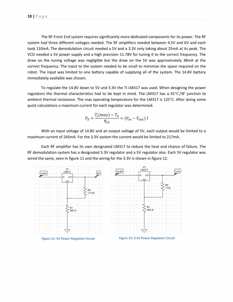
To regulate the 14.8V down to 5V and 3.3V the TI LM317 was used. When designing the power
regulators the thermal characteristics had to be kept in mind. The LM317 has a 41 junction to
ambient thermal resistance. The max operating temperature for the LM317 is 125°C. After doing some
quick calculations a maximum current for each regulator was determined.
( )
( )
With an input voltage of 14.8V and an output voltage of 5V, each output would be limited to a
maximum current of 245mA. For the 3.3V system the current would be limited to 217mA.
Each RF amplifier has its own designated LM317 to reduce the heat and chance of failure. The
RF demodulation system has a designated 3.3V regulator and a 5V regulator also. Each 5V regulator was
wired the same, seen in figure 11 and the wiring for the 3.3V is shown in figure 12.
Figure 11: 5V Power Regulator Circuit Figure 12: 3.3V Power Regulator Circuit

11 | P a g e
Figure 13: Proto Board of RF Amplifiers Regulators
The tune voltage was created using a potentiometer. This gave the ability to adjust the voltage
as the battery discharged. To improve the design a regulator would be used to create 12V and then a
voltage division to make 11.78V.
The power for the DUE was provided from a 9V battery. The due could be supplied with
anything from 6V to 16V. The 9V was used for the small form factor.
5.3. RF Front End System The RF Front End system was designed to detect, demodulate and give an accurate value of the
power received. The RF Front End System input was simple, as it was the modulated frequency shift key
(FSK) signal. The FSK signal had two frequencies, 2.15 GHz and 2.2 GHz. The baud of the FSK is 600 Bd.
The outputs were decided to be serial demodulated signal between 0 and 3.3V for the DUE to record
and a voltage level corresponding to the power received.

12 | P a g e
Figure 14: RF Front End System Block Diagram
The antenna supplied in class was tested and proved that it would work in this situation. The
power received was shown to be directional enough to be able to be able to detect when the antenna
was pointing at the beacon from the power received. The noise floor was measured at -70dBm with
signal strength of -40dBm when the antenna was directed at the beacon at a distance of 30-35 yards.
Rough angular power measurements were taken before the decision to use the antenna was used to
show that main lobe of the antenna was discernable enough to be able to distinguish when the antenna
was directly pointing at the beacon. After the build was complete, the antenna was again tested for
angular power received. The results that the Due measured are shown in figure 15. In this test, the Due
would measure the power inputted 150 times to get the most accurate measurement. It can be seen
that the power received is at 90° relative to the robot. The robot was positioned so that the beacon was
exactly 180° from the axis of travel. This test shows that without an abnormality measurement due to
noise that the Due would be able to discern where the beacon is with only about ±1° error.

13 | P a g e
Figure 15: Angular Power Received Plot
The desired power inputted was to be matched to the power output of the VCO. The power
output of the VCO is -7dBm meaning a gain of 33 dBm was needed. The amplifiers that were supplied,
Mini-Circuits ZFL-2500+, gave a gain of -25 dBm. The design originally went with dual stage amplification
and everything is set up to add a secondary amplifier to the system for longer detection. The current
design is only implementing a single stage amplifier. The power into the mixer after the amplification
stage is -15 dBm.
The down converting is done using a Mini-Circuit ZAM-42 frequency mixer. This inputted the
amplified signal and the VCO output to down convert to a 10.5 MHz signal. The VCO was tuned to 2.2105
GHz. The output is 2 frequencies still 50 MHz apart but now at 10.5 MHz and 60.5 MHz, with the lower
frequency representing the 2.2 GHz. The output is sent though a band pass filter to remove the 60 Mhz
signal. The output of the mixer and band pass filter is a 10.5 MHz signal that has a baud of 600 with the
code of the beacon encoded on it.

14 | P a g e
Figure 16: Output of Mixer and Band Pass Filter on Spectrum Analyzer
The RF Front End System demodulating is done on a proto board. The proto board gave higher
quality signals with less noise induced from longer jumper wires. The proto board could also be easily
unplugged and plugged in when needed for testing. The connectors that were chosen were Phoenix
Connector header connectors. The advantages of these connectors were closed leads and there were no
screws needed to make a secure connection. There was no chance of shorting if a cable assembly was
removed from the socket.
The band pass filter feeds the SMA jack that is located on the top shield. The AD8307
logarithmic amplifier was the crucial part of this design. The AD8307 inputted the signal and outputted a
voltage proportional to the inputted power. Since the 2.15 GHz signal was mixed down and filtered out,
the output of the log amp looked like a dirty version of the code emitted by the beacon. With a -45 dBm
input to the antenna the output of log amp was approximately 1.4V. The noise floor of -70 dBm was
represented with a 0.7V output.

15 | P a g e
Figure 17: AD8307 Log Amp Circuit
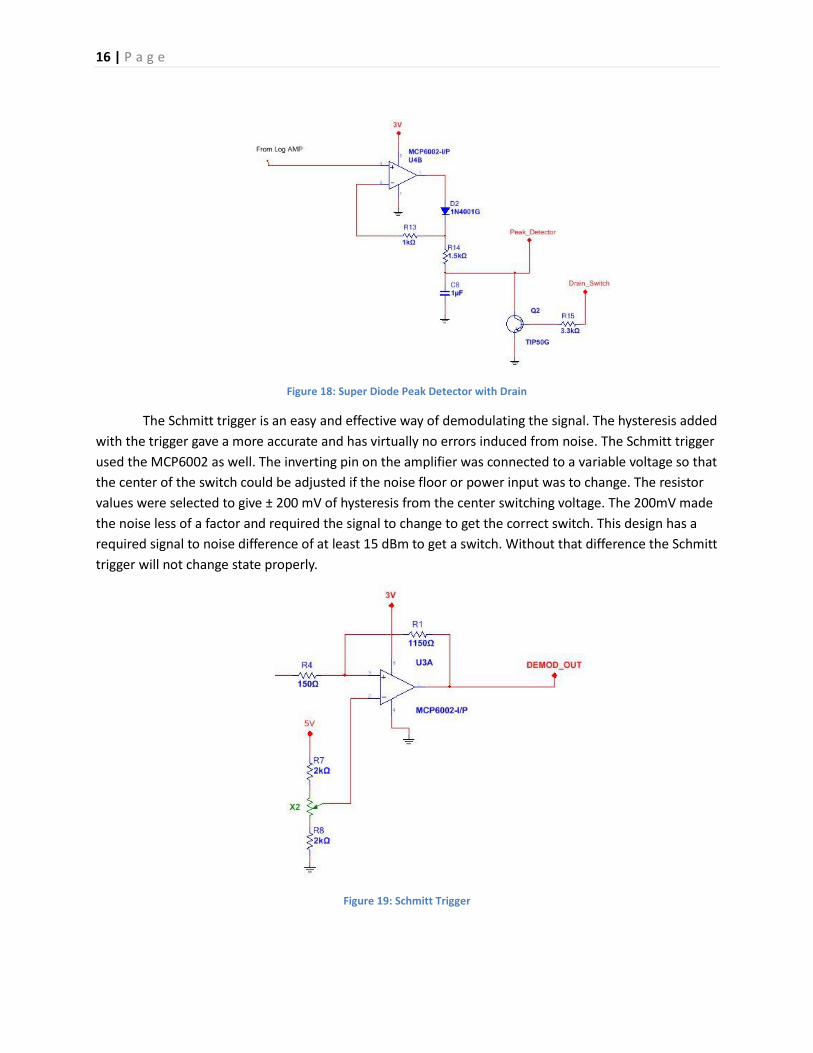
The peak detector and Schmitt trigger both used the output of the log amp. To increase the
resolution and ease of use an amplification stage of 1.5 was added after the log amp. The op-amp used
was the MCP6002 because it is a single ended supply that is rail to rail.
The peak detector was built using a super diode. The ability to quickly discharge the peak
detector was added using a TIP 42 PNP BJT. This ability gives a more accurate power measurement that is
less prone to noise disruptions that could occur when the antenna is swinging around. The peak detector
is built out of a 4.7µF capacitor and a 1kΩ resistor. The time constant for this pair is 4.7ms. To adequately
charge the peak detector without increasing the risk of noise being induced on the measurement a time
of 30mS would be needed from the time of the discharge to the time of reading. The time it takes to
discharge the capacitor is only 10µS.
16 | P a g e
Figure 18: Super Diode Peak Detector with Drain
The Schmitt trigger is an easy and effective way of demodulating the signal. The hysteresis added
with the trigger gave a more accurate and has virtually no errors induced from noise. The Schmitt trigger
used the MCP6002 as well. The inverting pin on the amplifier was connected to a variable voltage so that
the center of the switch could be adjusted if the noise floor or power input was to change. The resistor
values were selected to give ± 200 mV of hysteresis from the center switching voltage. The 200mV made
the noise less of a factor and required the signal to change to get the correct switch. This design has a
required signal to noise difference of at least 15 dBm to get a switch. Without that difference the Schmitt
trigger will not change state properly.
Figure 19: Schmitt Trigger

17 | P a g e
Figure 20: Output of RF Front End System
Figure 20 shows the outputs of the demodulation system. Channel 1 on the oscilloscope displays
the demodulation of the FSK signal. The Schmitt trigger outputs a 0V to 3.3V representing the code
inputted. Channel 2 show the peak detector with periodic drains of the capacitor. This test was run with
a beacon that was not tuned correctly. The beacon was emitting the correct signal but the lower
frequency was shifted up to 2.18 GHz. Even with this much smaller difference in shift the demodulation
circuit was able to demodulate the signal and give a high precision and accurate code. The peak detector
is seen charging and staying constant for approximately 100ms. It is then discharged and charged back
up to the same voltage. This test was done without moving the beacon or antenna and the peak
detector is shown to accurately reproduce the same voltage in reference to the same power received by
the antenna.
5.4. Control and Data Handling System In any robotic system, the Control and Data Handling portion of the design is extremely critical.
The Control and Data Handling System connects all other systems within the project together, allowing
for a well-integrated design.
The chosen Microcontroller board for the Beacon Buster was an Arduino Due seen in Figure 21.
The Due is an Arduino Board based on a 32-bit ARM core Microcontroller, the Atmel SAM3X8E ARM
Cortex-M3 CPU. The Arduino Due operates using CMOS technology. Therefore, the logic level for the
Due is 3.3V. With 54 Digital Input/Output ports (12 of which being PWM output capable), 12 Analog
Input ports, 2 Digital to Analog Converters, and 4 hardware serial ports, the Arduino Due was well suited
to control the Beacon Buster.

18 | P a g e
Figure 21: Arduino Due
From the down conversion stage of the RF Front End Subsystem, the Control and Data Handling
System must be capable of handling 600 Hz signals. The Arduino Due has a clock speed of 84 MHz which
is more than sufficient for the design and meets specification. As far as communication goes, the
Arduino Due has a SPI (Serial Peripheral Interface) header, IIC, and four pairs of hardware serial ports.
The Control and Data Handling System utilizes many of the Due's capabilities. The requirements of the
Control and Data Handling System are as follows:
Control Locomotion (this includes the rotation of the antenna)
Drain Peak Detector Capacitor
Record GPS Coordinates
Record measurements from the Peak Detector Circuitry
Record the Demodulated Signal from the Beacon
Save Data to micro-SD interface (Secure Digital non-volatile memory card)
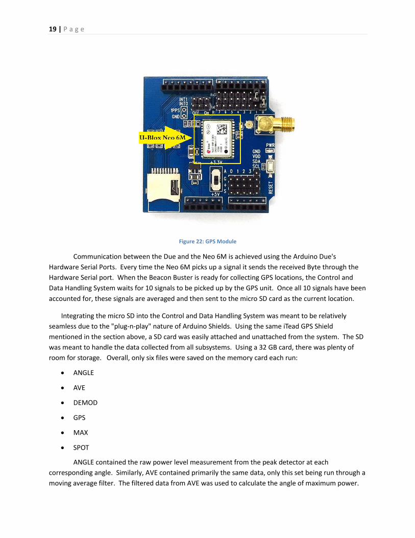
The GPS module chosen was a U-Blox Neo 6M paired with an active antenna. This GPS module was
purchased as a pre-assembled Arduino Shield from iTead Studios seen in Figure 22. The U-Blox Neo 6M
requires a 2.7-3.6V supply which is capable via the Arduino Due's regulated 3.3V supply. The Neo 6M
has an accuracy of 2.5 meters.
19 | P a g e
Figure 22: GPS Module
Communication between the Due and the Neo 6M is achieved using the Arduino Due's
Hardware Serial Ports. Every time the Neo 6M picks up a signal it sends the received Byte through the
Hardware Serial port. When the Beacon Buster is ready for collecting GPS locations, the Control and
Data Handling System waits for 10 signals to be picked up by the GPS unit. Once all 10 signals have been
accounted for, these signals are averaged and then sent to the micro SD card as the current location.
Integrating the micro SD into the Control and Data Handling System was meant to be relatively
seamless due to the "plug-n-play" nature of Arduino Shields. Using the same iTead GPS Shield
mentioned in the section above, a SD card was easily attached and unattached from the system. The SD
was meant to handle the data collected from all subsystems. Using a 32 GB card, there was plenty of
room for storage. Overall, only six files were saved on the memory card each run:
ANGLE
AVE
DEMOD
GPS
MAX
SPOT
ANGLE contained the raw power level measurement from the peak detector at each
corresponding angle. Similarly, AVE contained primarily the same data, only this set being run through a
moving average filter. The filtered data from AVE was used to calculate the angle of maximum power.

20 | P a g e
At each stop, the angle of maximum power was recorded in the MAX text file. Once the antenna is
pointing directly at the angle of maximum power, the Control and Data Handling System begins to
collect the data from the demodulation circuit. This data is recorded straight into the DEMOD file. The
GPS file contained the raw GPS coordinates at each stop. As mentioned in the GPS section, the Control
and Data Handling System collected ten measurements at each location. The average GPS coordinate at
each location was saved to the SPOT file. Using SPOT and MAX, the GPS location of the Beacon is easily
calculated using basic trigonometric identities discussed in section 5.5 below.
For the Peak Detector to work, the Control portion of the Control and Data Handling System was
needed to drain the capacitor before each power measurement. Before each and every measurement, a
3.3V 1 ms pulse was sent to the TIP 42 PNP BJT described in section 5.3. This pulse was implemented
utilizing one of the Arduino Due's Digital to Analog Converter. After a delay of 30 ms, the capacitor had
an ample amount of time to charge up to its maximum voltage which is proportional to the amount of
power received from the beacon. This measurement was collected five times at each angle and then
averaged. This averaged measurement was meant to eliminate unpredicted and incorrect
measurements. After saving the power measurements at each angle both on board and to the memory
card, these measurements were sent through a moving average filter to smooth out the curves. This
filter effectively cleaned up the data, eliminating unwanted spikes as seen below.
Figure 23: Peak Detector Sweep with Moving Average Filter
As the illustration above demonstrates, this moving average filter greatly enhances the Control
and Data Handling System's ability to find the true maximum peak by eliminating obviously incorrect
spikes and narrowing the beam width down to about 5 degrees. This immensely increases the accuracy
of the Beacon Buster by making each angle measurement more precise. This also helps with the
collecting of the demodulated signal.
The Demodulated Signal was collected through one of the Due's Analog Input Ports. This data
was sampled at the angle of maximum power at each location 5000 times. With a 25 microsecond delay
after each sample, each bit was roughly 60 samples long. This sampling rate was determined to read at
least five full message cycles from the beacon. Once all samples have been saved on board, this data
21 | P a g e
was transferred to the SD card. It is important to notice that the Demodulated Signal samples change at
a higher frequency that that of the Baud Rate for writing to the SD card, making it highly critical to save
the Demodulated Signal to the memory card after all samples have been read.
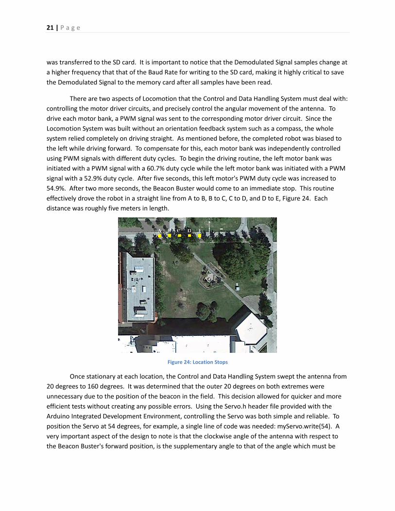
There are two aspects of Locomotion that the Control and Data Handling System must deal with:
controlling the motor driver circuits, and precisely control the angular movement of the antenna. To
drive each motor bank, a PWM signal was sent to the corresponding motor driver circuit. Since the
Locomotion System was built without an orientation feedback system such as a compass, the whole
system relied completely on driving straight. As mentioned before, the completed robot was biased to
the left while driving forward. To compensate for this, each motor bank was independently controlled
using PWM signals with different duty cycles. To begin the driving routine, the left motor bank was
initiated with a PWM signal with a 60.7% duty cycle while the left motor bank was initiated with a PWM
signal with a 52.9% duty cycle. After five seconds, this left motor's PWM duty cycle was increased to
54.9%. After two more seconds, the Beacon Buster would come to an immediate stop. This routine
effectively drove the robot in a straight line from A to B, B to C, C to D, and D to E, Figure 24. Each
distance was roughly five meters in length.
Figure 24: Location Stops
Once stationary at each location, the Control and Data Handling System swept the antenna from
20 degrees to 160 degrees. It was determined that the outer 20 degrees on both extremes were
unnecessary due to the position of the beacon in the field. This decision allowed for quicker and more
efficient tests without creating any possible errors. Using the Servo.h header file provided with the
Arduino Integrated Development Environment, controlling the Servo was both simple and reliable. To
position the Servo at 54 degrees, for example, a single line of code was needed: myServo.write(54). A
very important aspect of the design to note is that the clockwise angle of the antenna with respect to
the Beacon Buster's forward position, is the supplementary angle to that of the angle which must be

22 | P a g e
written to the Servo. For example, to position the antenna 20 degrees from forward, an angle of 160
degrees must be written to the Servo.
5.5. Post-Processing System The Post-Processing Subsystem was designed to process and interpret the data collected from
the Control and Data Handling Subsystem and output the results in an efficient, easy to read manner.
Thus, the inputs to the Post-Processing Subsystem were the data which was collected from the Control
and Data Handling Subsystem. This included the GPS coordinates at each location, the angle of max
power at each location, and the decoded FSK signal at the angle of max power. Using sophisticated
algorithms, as well at the data inputs, the outputs of the Post-Processing Subsystem were the GPS
coordinates of the beacon in the courtyard, as well as the decoded FSK signal, represented using eight
bits (ones or zeroes).
As mentioned earlier, to implement the Post-Processing Subsystem we used two sophisticated
algorithms. The first of these algorithms was used to process the data taken from the analog to digital
converter which was recording the decoded signal. When creating this algorithm, we had to take many
factors into account. The first of these factors was that the analog to digital converter (which was a 10
bit ADC) gave values of 1000-1024 for a high and values of 0-20 for a low, although we wanted out signal
in 1s and 0s. To change this, we used a threshold and a for loop that ran through the collected data
which would turn all of the values above 512 (half of 1024) to 1s (high) and all the values below 512 to
0s (low). Thus, we had an array of only 0s and 1s. The next factor we had to take into account was the
sampling rate at which we collected data relative to the baud rate of the FSK signal, which was 600 Bd.
To control the rate at which we sampled the decoded signal, we used delays in our code between each
sample. Thus, we were able to control the amount of data points that were collected per bit. We found
that with a 25 millisecond delay we were able to collect 60 data points per bit. Another factor we had to
take into account was where we started collecting data. More often than not we would begin in the
middle of a bit. Also, we could start collecting data in the middle of our signal. To counter these facts,
we decided that we must find the location in our decoded signal of the first data point of the start bit,
which would be a zero. To do this, we looked at the first data point collected. If the first data point
collected was a one, we would then delete all of the ones in front of it until we got to a zero. We would
then delete the next ten bits (600 data points). This ensured that even if we began in the middle of our
signal the program would not get confused. After deleting the next ten bits we would always land on a
one. We would then delete all of the ones until we got to a zero again. This zero would always be the
first data point of the start bit. If instead our first data point collected was a zero, we would start by
deleting the first ten bits (600 data points) which would always take us to a one. We would then delete
all of the ones until we got to a zero, which would be the first data point of the start bit. Now that we
were insured that we started at the first data point of the start bit, we would then average 60 data points
in subsequent order and then round the value we got. Thus, we would average the first 60 data points
and round the value, and save it, then we round the next 60 data points, round the value, and save it
again. If we did this nine times we would get our decoded signal out, including the start bit. This

23 | P a g e
algorithm was created in the way that it was to ensure that it was a robust system in which the signal we
were decoding did not matter, nor did the location at which we began collecting data mattered.
The next algorithm we implemented was the triangulation algorithm, which was used to locate
the beacon. Using figure x the algorithm will be explained.
Figure 25: Triangulation Method
The steps of this algorithm are fairly straight forward. We know all of the angles, as well as the distance
between each points. We use the distance (labeled x) and two subsequent angles theta(n) and
theta(n+1), as well as the Law of Sines to find the hypotenuse for each triangle. Once we have that data,
we use the hypotenuse of each triangle to find an xtot and ytot. Depending on if the angle theta(n) is less
than 90 degrees or greater than 90 degrees, we do different calculations. If theta(n) is less than 90
degrees, then we just use sine and cosine to find xtot and ytot. From the figure, we see that ytot(n) =
hyp(n)*sin(theta(n)). Also from the figure, we see that xtot = hyp(n)*cos(theta(n)) + x*(n-1). We have to
add x*(n-1) because if we do not we just get the adjacent length of the triangle that theta(n) makes,
rather than all of xtot. If theta(n) is greater than 90 degrees we do very similar calculations, the only
difference comes from the fact that the angles used in our triangles are going to be 180 minus our
obtained angle. Using this consideration, we can find xtot and ytot for these locations as well. Now, if the
angle is equal to 90 degrees, then our xtot value is just our obtained location and our ytot value is the
hypotenuse obtained from earlier. Thus, xtot = x(n) and ytot = hyp(n). We now have values for xtot and ytot
at each of the locations. The values should all be fairly close to each other. Thus, we then average all of
the values to get our final value. Something to note is that these calculations are with respect to a
starting point of (0,0) on the (x,y) axis. Thus, to get the correct location we must offset our final answer
by the location of our starting point. Another note is that we applied this algorithm to an array which
represented the pixels of an image (the courtyard). To get the GPS coordinates from this array we used a
conversion factor from our x values of the array and our y values of the array. Thus, we took our GPS
coordinates at each location, converted these locations to the pixel values of the image, applied the
triangulation algorithm to the pixel values which gave us a single pixel, and then converted this pixel
value back into a GPS value.

24 | P a g e
The two preceding algorithms were created and tested on MATLAB. Using these two algorithms,
we were able to find both the GPS coordinate of the beacon as well as interpret and display the eight
bits of the decoded FSK signal. We wanted to be able to read the processed results in an efficient, easy
to read manner. To accomplish this goal we decided to implement a Graphical User Interface using
Visual BASIC. We converted the MATLAB code to BASIC code with ease, with problems only arising from
the change of index between the two languages. This turned out to be an excellent idea, as the ease of
the GUI is notable. Figure x is an image of the GUI.
Figure 26: Custom Graphical User Interface
The GUI has four clickable buttons as well as three input parameters. The first parameter is used to
change the amount of data points per bit, if we were able to change that in the Control and Data
Handling Subsystem. The next parameter changes the amount of locations we stopped at, while the last
value changes the threshold at which to change the values from the ADC to 1s and 0s. The top left
button, the bottom left button, and the bottom right button are used to load the location data at each
stop, the decoded signal data, and the angle of max power data at each stop, respectively. Clicking each
of these buttons will allow us to choose the data from the SD card on the computer. When we press the
top right button, labeled “Triangulate,” we get the desired outputs displayed on the GUI. Figure x
illustrates what occurs after “Triangulate” is pressed.

25 | P a g e
Figure 27: GUI with Recorded Data
As you can see, all of the data we desired is displayed on the GUI. In the top left corner we have the
GPS location of the beacon displayed in longitude and latitude. On the image of the courtyard we see
our three stops on the map, as well as the angle at which the angle of max power was recorded for each
stop. Also on the image we see a yellow circle, which is placed where the GPS location of the beacon
should be. For this data set, we had the beacon on a table, and the yellow circle is very close to the
table. Thus, we are very accurate and precise. To the upper right we see that the GPS locations and the
angles of max power are saved in a table, and to the lower right we see our collected data from the ADC
for the decoded signal. Also, above this plot of the ADC data we see the output from our first algorithm,
which is a 9 bit (including the start bit) binary representation of the FSK signal. Similar results occur if we
change the location of the beacon or the FSK signal being emitted by the beacon. The Graphical User
Interface was very helpful because it allowed us to load the data in a very smooth, easy manner, and it
displayed the results in a manner which was easy to interpret and efficient to use.
The results from the Post-Processing Subsystem are exactly what we expect. The system produces the
exact results which we desired, which were the GPS coordinates of the beacon as well as the 8 bit
representation of the encoded FSK signal.

26 | P a g e
6. Budget Table 1: Budget
Part Cost
Arduino Due $39.99
GPS Shield $57.99
Chassis Material $44.50
Arduino Protoboards 2x19.99 = $39.98
Circuit Components $54.60
Servo $11.79
Miscellaneous Parts $50
Total $298.85
7. Timeline Table 2: Timeline
Date Task Completed
February 4, 2014 Parts Ordered and Chassis Complete February 13, 2014 Conceptual Design Review February 14, 2014 Locomotion Run March 1, 2014 Began RF System Design and Order Parts March 11, 2014 Midterm Functionality and Design March 15, 2014 Began Implementation of GPS and Algorithms April 1, 2014 Breadboard Power and RF System Together April 15, 2014 Begin Soldering of Circuits on Proto boards April 22, 2014 Integrate GPS, Algorithms, Due Code, and GUI together April 24, 2014 Soldered/Tested Circuits on Due Proto boards April 26, 2014 Integration of all subsystems April 28, 2014 Fully Functional, Testable Robot April 29, 2014 Final Functionality and Design May 1, 2014 Final Presentation May 6, 2014 Final Report
8. Testing The majority of the testing happened before the final integration. Knowing the inputs and outputs of
each subsystem and the interconnects between the subsystems before the design of each individual
system, each of the inputs could be simulated accurately to test the system without needing to have
every subsystem built. This reduced testing time required once the whole robot was built.

27 | P a g e
The locomotion and chassis system was tested fully once the complete robot was assembled. The
custom chassis was built and verified to fit and the ball bearing was spun to verify that it provided a low
resistance 180° rotation.
The testing of the power system was easy to simulate in the lab. Each regulator was built and loaded
either with the load or a simulated load. The motor driver was tested using the chassis and the Due for
the control signal. This test also gave a rough power draw of the motors. There was an error in this
measurement because the robot was not fully loaded. The testing of the regulators was done by
simulating the load with the actual amplifiers. The demodulating power regulators were tested by
simply connecting them to a 100Ω load.
The RF system testing was done using the beacon and the antenna. This input was harder to
simulate than other inputs. The whole circuit was built on a bread board and was tested. The output was
verified to work using an oscilloscope. The bread board gave the ability to change low pass filters and
different gains on the amplifiers. This testing gave the final values of each filter and gain making testing
once the circuit was on a proto board very simple.
The control and data handling was tested using a function generator to simulate the inputs from the
RF front end system. The GPS had to be tested outside to receive an accurate signal but the relied on no
other input so it could be tested fully without any other system. The same went with the SD card. The
testing was done using simulated data. The rotation of the antenna and movement was done in the lab.
This gave a close to accurate values on driving straight. The final testing was performed outside to
ensure the linear movement translated to the outside on a different surface. Some tweaking had to be
done to correct for drifts once a full cycle was performed.
The testing of the post processing was simple and effective. The output of the control and data
handling system was very easy to simulate. This was fed into the GUI and shown to work. By changing
the input slightly the GUI was shown to effectively process the data and parse it into useful information.
The testing of the whole system was fairly simple once the other systems were proven to work. The
MCP6002 failed several times while doing a full test. This caused issues with over drawing the power
system and under powering other components. After the third MCP6002 failed after working in the RF
front end system individually, the thought was that static discharge was causing the failure. More
filtering capacitors were added to the system and an amplifier prone to failure was moved to the lower
shield so that there was less chance of a static discharge from a tester touching it while plugging and
unplugging cables.
9. Final Results The Beacon Buster was finished by the deadline of May 1st. It was shown to accurately locate the
beacon and demodulate the signal emitted from the beacon. The final build is seen in section 5.1. The
Beacon Buster has repeatedly been tested with different beacons and with different location. The tests

28 | P a g e
have always been within the margin of error with the demodulation always working when the robotis in
tune.
10. Conclusion In the technological age, the way we as a species complete tasks becomes increasingly
automated and repeatable. It allows us to go beyond what we had originally thought possible, with
ideas only our imaginations could conjure.
We were tasked with creating a piece of technology which needed to autonomously perform
several tasks, and do these tasks in an efficient, precise, and reliable manner. The Beacon Buster was to
autonomously locate a beacon emitting a Frequency Shift Key signal, as well as decode that signal. It
met these goals, as it can produce the GPS coordinates of the beacon within a very reasonable range of
ten meters, as well as decode the FSK signal. The location of the beacon does not matter, nor does the
encoded message of the FSK signal, for the Beacon Buster to complete its task.
The task of completing the Beacon Buster was subject to many constraints. The first constraint
was to have a reliable, working robot by May 1, 2014. This constraint was met, as the robot was
completed by April 29, 2014. The next constraint was that the robot must be completed within a budget
of $325. As evidence from our accurate budget table, we spent ~$300, which allowed us to meet our
budget constraint. The third constraint was that we must include a custom part in our design when
completing the Beacon Buster. We not only included one custom part, but many. We had a custom
chassis, custom MOSFET motor drivers, a custom power system, a custom circuit for demodulation, and
a custom Graphical User Interface. Thus, our third and final constraint was met beyond expectation.
We met all of the goals asked of us subject to all of the constraints. The Beacon Buster is a reliable
robot which can produce the GPS coordinates and the demodulated message from the FSK signal
repeatedly and accurately. The Beacon Buster can be picked up and used by anyone due to its ease of
use, but can also be used for more complex, analytically manners due to its sophistication. As a
prototype for future designs and manufacturing purposes, the Beacon Buster is an optimal choice for
automated, beacon finding, and code cracking consumers.

29 | P a g e
11. Appendices
Appendix A: Final Code for Robot #include <SPI.h>
#include <SD.h>
#include <TinyGPS.h>
#include <Servo.h>
TinyGPS gps;
/
THIS IS THE COMPLETED TEST CODE FOR BEACON BUSTER
*/
//////////////////////////PINOUT//////////////////////////////
////Digital////
//13:SPI(CLK)
//12:SPI(MOSI)
//11:SPI(MISO)
//10:SPI (CS)
//9:SERVO
//8:
//7:
//6:
//5:Left HBridge
//4:Right HBridge
//3:GPS SERIAL RECEIVE
//2:GPS SERIAL TRANSMIT

30 | P a g e
//1:SERIAL
//0:SERIAL
////Analog////
//A0:Demod In
//A1:PWR Detect In
//DAC1:
//DAC2:
//Digital Declarations
int leftMotorPin = 4; //Left HBridge
int rightMotorPin = 5; //Right HBridge
int Analog0 = 0; //Demod In
int Analog1 = 1; //PWR Detect In
////////////////////////PINOUT END////////////////////////////
//The Arduino Due has three 3.3V TTL serial ports: Serial1 on pins 19(RX) and 18 (TX);
Servo myServo;
//int motPin = 8;
int angle;
//int angles[180];
int peakVal;
int maxPeak = 0;
int maxPeakVal = 0;
int peak2;
int t; //average angle vals
int peaks[140];

31 | P a g e
int findpeak[140];
int m;
//For Demod
int demod;
int k;
int array[5000];
//GPS
float latt;
float longg;
int i; //Number of GPS Locations Loop
int j; //Number of Stops Loop
int runtest = 1; //Run Test Condition
/**************************************************************
Function: setup
Purpose: set up Arduino
Args: none
Returns: nothing
Notes: This function is required by the Arduino
***************************************************************/
void setup()
//Turn off power to motors
analogWrite(leftMotorPin,0); //Drive at half speed
analogWrite(rightMotorPin,0); //Drive at half speed
delay(2000);

32 | P a g e
//Connect Servo
myServo.attach(9);
// Serial monitor
Serial.begin(9600);
// baud rate for GPS - 38400 is prefered, but 4800 can also be used
Serial1.begin(38400); //Serial1 on pins 19(RX) and 18 (TX)
// Initialize card
Serial.print("Initializing SD card...");
pinMode(10, OUTPUT);
if (!SD.begin(10))
Serial.println("...initialization failed!");
else
Serial.println("...initialization done.");
/**************************************************************
Function: loop
Purpose: loop funtion for Arduino
Args: none
Returns: nothing
Notes: This function is required by the Arduino, and the
Arduino will loop through this function indefinately.

33 | P a g e
***************************************************************/
void loop()
if (runtest ==1)
//for (j=0;j<3;j++)
for (j=0;j<5;j++)
/////////////////////////////GPS////////////////////////////////////////////////
File GPSdata = SD.open("GPS.txt", FILE_WRITE);
GPSdata.println("Start");
GPSdata.close();
latt = 0; //Redeclare
longg = 0;
for (i=0;i<=10;i++)
bool newData = false;
unsigned long chars;
unsigned short sentences, failed;
// Open data file
File GPSdata = SD.open("GPS.txt", FILE_WRITE);
int gett = 1;
int incomingByte = Serial1.read();
while (gett == 1)
/////////////////////////////////////////
if (Serial1.available() > 0)
incomingByte = Serial1.read();

34 | P a g e
if (gps.encode(incomingByte))
gett = 0;
float flat, flon;
unsigned long age;
gps.f_get_position(&flat, &flon, &age);
GPSdata.print(flat == TinyGPS::GPS_INVALID_F_ANGLE ? 0.0 : flat*1000000);
latt = latt + (flat == TinyGPS::GPS_INVALID_F_ANGLE ? 0.0 : flat);
GPSdata.print(",");
GPSdata.print(flon == TinyGPS::GPS_INVALID_F_ANGLE ? 0.0 : flon*1000000);
longg = longg + (flon == TinyGPS::GPS_INVALID_F_ANGLE ? 0.0 : flon);
//if gps.encode(encomingByte)
//if serial1.available()>0
//////////////////////////////////////////
//while gett = 1;
GPSdata.println("");
GPSdata.close();
//for i = 0
latt = (latt/11)*1000000; //Average Latitude (these both are Integers so we multiply by a factor of
10^6 and divide by the same factor in post processing)
longg = (longg/11)*1000000; //Average Longitude
File Locationdata = SD.open("Spot.txt", FILE_WRITE);
if (Locationdata)

35 | P a g e
Locationdata.print(latt);
Locationdata.print(",");
Locationdata.println(longg);
Locationdata.close();
//////////////////////////////////GPS END//////////////////////////////////////
//////////////////////////////////Servo////////////////////////////////////////
angle = 160;
m = 0;
File Angledata = SD.open("Angle.txt", FILE_WRITE);
if (Angledata)
Angledata.println("Start");
Angledata.close();
while(angle!=20)
myServo.write(angle); //Rotate Servo
analogWrite(DAC1,255); //1ms pulse to discharge peak capacitor
delay(1); //
analogWrite(DAC1,0); //30ms low to charge up peak capacitor
delay(30);
peakVal = analogRead(Analog1);
for(t=0;t<4;t++)
analogWrite(DAC1,255); //1ms pulse to discharge peak capacitor
delay(1); //

36 | P a g e
analogWrite(DAC1,0); //30ms low to charge up peak capacitor
delay(30);
peakVal = peakVal + analogRead(Analog1);
peakVal = peakVal / 5;
peaks[m] = peakVal;
File Angledata = SD.open("Angle.txt", FILE_WRITE);
if (Angledata)
Angledata.println(peakVal);
Angledata.close();
m++;
angle--;
///////////Moving Average Filter//////////////////
File Avedata = SD.open("Ave.txt", FILE_WRITE);
if (Avedata)
Avedata.println("Start"); //Write "Start" to Ave.txt
Avedata.close();
for(m=0;m<140;m++)
if(m<5 )
findpeak[m] = 0;
37 | P a g e
else if (m>134)
findpeak[m] = 0;
else
findpeak[m] = (peaks[m-5] + peaks[m-4] + peaks[m-3] + peaks[m-2] + peaks[m-1] + peaks[m] +
peaks[m+1] + peaks[m+2] + peaks[m+3] + peaks[m+4] + peaks[m+5] )/11;
if(findpeak[m] > maxPeakVal)
maxPeakVal = findpeak[m]; //save the maxPeakVal for peak comparison
maxPeak = 160-m; //save the max angle
File Avedata = SD.open("Ave.txt", FILE_WRITE);
if (Avedata)
Avedata.println(findpeak[m]); //Record the Averaged Peak Detector Data
Avedata.close();
///////////Moving Average Filter END//////////////////
File Maxdata = SD.open("Max.txt", FILE_WRITE);
if (Maxdata)
Maxdata.println(maxPeak); //Record the MAX PEAK ANGLE to MAX.txt
Maxdata.close();
//Return the Servo to maxPeak in increments of 1 degree every .2 seconds

38 | P a g e
angle = angle + 1;
while(angle!=maxPeak)
myServo.write(angle);
delay(200);
angle++;
////////Demod///////////////
//Save demod signal to array
for(k=0;k<4999;k++)
array[k] = analogRead(Analog0);
delayMicroseconds(25); //A 25microSecond Delay should create a 60dp/bit message, recording about
5400 dp = 6 messages
//Send demod signal to SD
for(k=0;k<4999;k++)
File Demoddata = SD.open("Demod.txt", FILE_WRITE);
if (Demoddata)
Demoddata.println(array[k]);
Demoddata.close();
//////Demod END////////////
//Return the Servo to home
angle = angle + 1;
39 | P a g e
while(angle!=160)
myServo.write(angle);
delay(200);
angle++;
maxPeakVal = 0; //Redeclare maxPeakVal = 0
delay(1000);
//////////////////////////////////Servo END////////////////////////////////////
/////////////////////////////////////Drive/////////////////////////////////////
analogWrite(leftMotorPin,155); //Drive at half speed
analogWrite(rightMotorPin,135); //Drive at half speed
delay(5000); //Continue for x ms
analogWrite(leftMotorPin,155); //Stop 150
analogWrite(rightMotorPin,140); //Stop 150
delay(2000);
analogWrite(leftMotorPin,0); //Stop
analogWrite(rightMotorPin,0); //Stop
delay(1000); //Pause for x ms
/////////////////////////////////////Drive END///////////////////////////////////
//for j = 0 to 4
runtest = 0;
//if runtest = 1
analogWrite(leftMotorPin,0); //Stop

40 | P a g e
analogWrite(rightMotorPin,0); //Stop
delay(1000); //Pause for x ms
//Main Loop
/*PSUEDO CODE
1:Initialize Variables
2:Set-up
3:Average GPS Data (Write To GPS file)
Sweep Servo/Record peakValues
Return Serov to Max Peak
Save Signal Data (Write to Signal file)
Return Servo
4:Drive for x-seconds
5:Repeat from Step 3
*/
Appendix B: MATLAB Codes
Triangulation: function [xo,yo] = triangulatetest(x,y,angle) %A MATLAB function which finds the x and y coordinates of point using the %angles the point makes with a straight path at several known locations %x is a list of x coordinates at several locations %y is a list of y coordinates at several locations %angle is the angle that points directly at the location we are trying to %find from the (x,y) point with respect to a linear path %xo is the x coordinate of the loaction we are trying to triangulate %yo is the y coordinate of the loaction we are trying to triangulate
41 | P a g e
%we use n to find the length n = length(x);
%we initialize these vectors filled with zeroes for speed %xlength is one element shorter because it measures the lengths between %subsequent x values, and thus there is one less distance then there are %points hyp = zeros(size(x)); xlength = zeros(length(x) - 1); ytot = zeros(size(y)); xtot = zeros(size(y));
%this gets the distance between each x value and saves it into xlength for i = 1:n-1
xlength(i) = x(i+1) - x(i);
end
%this produces the first hypotenuse value using the Law of Sines hyp(1) = xlength(1)*(sind(180 - angle(2))/sind(angle(2) - angle(1)));
%again using the Law of Sines we find all of the hypotenuse values for i = 2:n
hyp(i) = xlength(i-1)*(sind(angle(i-1))/sind(angle(i) - angle(i - 1)));
end
%here, we calculate xtot and ytot, which are the x and y coordinates found %for the coordinate we are searching for (we will then average them) for i = 1:n
%if the angle is less than 90 degrees we use sine to find ytot and xtot if angle(i) < 90
ytot(i) = hyp(i)*sind(angle(i)); xtot(i) = hyp(i)*cosd(angle(i));
%we are not completely done with xtot because we also have to add %the previous values for xlength to xtot to get all of xtot for j = 2:i
xtot(i) = xtot(i) + xlength(j-1);
end
%if the angle is greater than 90 degrees we do something very similar %to the above process just with the angle subtracted by 180 elseif angle(i) > 90

42 | P a g e
ytot(i) = hyp(i)*sind(180 - angle(i)); xtot(i) = hyp(i)*(sind(angle(i) - angle(1))/sind(angle(1)) - cosd(180
- angle(i)));
%if the angle is equal to 90 degrees than we have that xtot is equal to %x value we have and ytot is equal to the hypotenuse measured else
ytot(i) = hyp(i); xtot(i) = x(i);
end
end
%we now have an array called xtot and ytot filled with values for our %output. We average the values in each array and set them equal to our %outputs yo = mean(ytot); xo = mean(xtot);
end
Demodulation: function [decoded] = decodesig(x,approximate_datapoints) %A MATLAB function which takes the values from the ADC that is collecting %the data from the demodulation circuit and outputs the signal in a 9 bit %(including the start bit) representation of binary zeroes and ones. %x is the data obtained from the ADC %approximate_datapoints is the approximate amount of datapoints which %represent each bit %decoded is the output, which gives the message from the FSK in a 9 bit %format of zeroes and ones
%here, we find n so that we could loop through x n = length(x);
%we initialize the decoded array for speed decoded = zeros(1,9);
%this bloack changes all of the values of the array x that are above 512 %to 1 and below 512 to 0 y = find(x<512); encoded = ones(1,n); encoded(y) = x(y); encoded(y) = 0;
%we use a ten percent error of our approximate datapoints to find the exact %amount of datapoints per bit tenperror = round(.1*approximate_datapoints);

43 | P a g e
%these are used to check whether values are zeroes or ones in the next %block of code check1 = 1; count1 = 0; check2 = 1; count2 = 0; check3 = 1; count3 = 0; check4 = 0; count4 = 0;
%we check what value we start with which depends on if encoded(1) == 1
%if we begin with a one, we delete ones until we get to a zero while check1 == 1
count1 = count1+1; check1 = encoded(count1);
end
%which is what we do here encoded(1:count1-1) = [];
%this deletes the next 10 bits which will effectively put us in ones %again encoded(1:10*approximate_datapoints) = [];
%and here, we delete all of the ones until we get to a zero again, %which will always be our start bit while check2 == 1
count2 = count2+1; check2 = encoded(count2);
end
encoded(1:count2-1) = [];
else
%if we start of with a zero, we immediately delete the next ten bits %which will put us in ones again encoded(1:10*approximate_datapoints) = [];
%we then delete ones until we get to the start bit (0) while check3 == 1
count3 = count3+1; check3 = encoded(count3);

44 | P a g e
end
encoded(1:count3-1) = [];
end
%we then check how many zeroes are present while check4 == 0
count4 = count4+1; check4 = encoded(count4);
end
count4 = count4 - 1;
%using the amount of zeroes presetn and the approximate data points in a %bit, we use this block to determine the exact amount of datapoints in %each bit for j = 1:8
if count4<(approximate_datapoints+tenperror)*j
if count4>(approximate_datapoints-tenperror)*j
datapoints = round(count4/j);
end
end
end
%we check from 1 to datapoints, and take the average of these values, and %round it up decoded(1) = round(mean(encoded(1:datapoints)));
%we then do the same average the round for each block of datapoints for i = 2:9
decoded(i) = round(mean(encoded((i-1)*datapoints:i*datapoints))); end %this effectively gives our output as a 9 bit binary message end
Appendix C: Visual Basic Codes Public Class Form1 'Initialize Variables Dim lat As Double Dim lng As Double

45 | P a g e
Dim x0 As Integer = 18 Dim y0 As Integer = 124 Dim x0_long As Double = -106.907817 Dim y0_lat As Double = 34.066976 Dim conv As Double = 0.0000015 'Conversion factor for converting longitude to pixel (x) Dim yconv As Double = 0.00000124'Conversion factor for converting latitude to pixel (y) Dim xval As Integer Dim yval As Integer Dim x1_long As Double = -106.906827 Dim y1_lat As Double = 34.066386 #Region "Triangulate" Private Sub TriangulateButton_Click(sender As System.Object, e As System.EventArgs) Handles TriangulateButton.Click Dim xx(TextBox2.Text - 1) As Integer Dim yy(TextBox2.Text - 1) As Integer Dim ang(TextBox2.Text - 1) As Integer Dim angrad(TextBox2.Text - 1) As Double 'This Sub is activated once the Triangulation Button is Clicked. 'It loads up the previously declared variables, xx,yy,ang,angrad with the data ' from the Data Grid. It also positions the yellow boxes according to ' their Latitude and Longitude which uses the conversion factor to convert ' to pixels position on the image. From here, we also use the angles at each ' location to draw a yellow line across the image with the corresponding angle ' This displays their intersections based off of the angles and gps coordinates ' to provide a visual aide when viewing our data lat = DataGridView1.Rows(0).Cells(1).Value lng = DataGridView1.Rows(0).Cells(2).Value xval = Math.Round((lng - x0_long) / conv) yval = Math.Round((y0_lat - lat) / yconv) Position1.Location = New Point(xval, yval) Position1.BringToFront() xx(0) = xval yy(0) = yval ang(0) = DataGridView1.Rows(0).Cells(3).Value Line1.X1 = xval Line1.Y1 = yval Line1.Y2 = 600 Line1.X2 = 1 / Math.Tan(ang(0) * Math.PI / 180) * (600 - yval) + xval '///////////////////////////////////////////////////////////////////////////// lat = DataGridView1.Rows(1).Cells(1).Value lng = DataGridView1.Rows(1).Cells(2).Value

46 | P a g e
xval = Math.Round((lng - x0_long) / conv) yval = Math.Round((y0_lat - lat) / yconv) Position2.Location = New Point(xval, yval) Position2.BringToFront() xx(1) = xval yy(1) = yval ang(1) = DataGridView1.Rows(1).Cells(3).Value Line2.X1 = xval Line2.Y1 = yval Line2.Y2 = 600 Line2.X2 = 1 / Math.Tan(ang(1) * Math.PI / 180) * (600 - yval) + xval '//////////////////////////////////////////////////////////////////////////// lat = DataGridView1.Rows(2).Cells(1).Value lng = DataGridView1.Rows(2).Cells(2).Value 'Position3.Location = New Point(lat, lng) xval = Math.Round((lng - x0_long) / conv) yval = Math.Round((y0_lat - lat) / yconv) Position3.Location = New Point(xval, yval) Position3.BringToFront() xx(2) = xval yy(2) = yval ang(2) = DataGridView1.Rows(2).Cells(3).Value Line3.X1 = xval Line3.Y1 = yval Line3.Y2 = 600 Line3.X2 = 1 / Math.Tan(ang(2) * Math.PI / 180) * (600 - yval) + xval '////////////////////////////////////////////////////////////////////////// 'Try If TextBox2.Text = "4" Or TextBox2.Text = "5" Then lat = DataGridView1.Rows(3).Cells(1).Value lng = DataGridView1.Rows(3).Cells(2).Value xval = Math.Round((lng - x0_long) / conv) yval = Math.Round((y0_lat - lat) / yconv) Position4.Location = New Point(xval, yval) Position4.BringToFront() xx(3) = xval yy(3) = yval ang(3) = DataGridView1.Rows(3).Cells(3).Value Line4.X1 = xval Line4.Y1 = yval Line4.Y2 = 600 Line4.X2 = 1 / Math.Tan(ang(3) * Math.PI / 180) * (600 - yval) + xval Line4.Show() Line4.BringToFront() Position4.Show() Else Line4.Hide() Position4.Hide() End If If TextBox2.Text = "5" Then lat = DataGridView1.Rows(4).Cells(1).Value

47 | P a g e
lng = DataGridView1.Rows(4).Cells(2).Value xval = Math.Round((lng - x0_long) / conv) yval = Math.Round((y0_lat - lat) / yconv) Position5.Show() Position5.Location = New Point(xval, yval) Position5.BringToFront() xx(4) = xval yy(4) = yval ang(4) = DataGridView1.Rows(4).Cells(3).Value Line5.X1 = xval Line5.Y1 = yval Line5.Y2 = 600 Line5.X2 = 1 / Math.Tan(ang(4) * Math.PI / 180) * (600 - yval) + xval Line5.Show() Line5.BringToFront() Else Line5.Hide() Position5.Hide() End If 'Convert our degree angles to radians For i As Integer = 0 To TextBox2.Text - 1 '2 angrad(i) = ang(i) * Math.PI / 180 Next Try Triangulate(xx, yy, angrad) 'Do Triangulate Function Catch ex As Exception MsgBox("Error! Check Number of Locations") End Try End Sub Function Triangulate(ByVal x() As Integer, ByVal y() As Integer, ByVal angle() As Double) As Double 'View MATLAB CODE, this function is the same, only converted to VB.Net Dim n As Integer = x.Length - 1 Dim hyp(n) As Double 'hyp(4) Dim xlength(n - 1) As Double '0 1 2 3 Dim ytot(y.Length - 1) As Double Dim xtot(y.Length - 1) As Double Dim xo As Double = 0 Dim yo As Double = 0 For i As Integer = 0 To n - 1
48 | P a g e
xlength(i) = x(i + 1) - x(i) Next hyp(0) = xlength(0) * (Math.Sin(Math.PI - angle(1)) / Math.Sin(angle(1) - angle(0))) For i As Integer = 1 To n hyp(i) = xlength(i - 1) * (Math.Sin(angle(i - 1)) / Math.Sin(angle(i) - angle(i - 1))) Next For i As Integer = 0 To n If angle(i) < Math.PI / 2 Then ytot(i) = hyp(i) * Math.Sin(angle(i)) xtot(i) = hyp(i) * Math.Cos(angle(i)) For j As Integer = 1 To i xtot(i) = xtot(i) + xlength(j - 1) Next ElseIf angle(i) > Math.PI / 2 Then ytot(i) = hyp(i) * Math.Sin(Math.PI - angle(i)) xtot(i) = hyp(i) * (Math.Sin(angle(i) - angle(0)) / Math.Sin(angle(0)) - Math.Cos(Math.PI - angle(i))) Else ytot(i) = hyp(i) xtot(i) = x(i) End If Next For k As Integer = 0 To n xo = xtot(k) + xo yo = ytot(k) + yo Next xo = Math.Round(xo / (n + 1)) yo = Math.Round(yo / (n + 1)) Dim xspot As Integer = xo + x(0) Dim yspot As Integer = yo + y(0) Dim xlong As Double = xspot * conv + x0_long Dim ylat As Double = y0_lat - yspot * yconv Dim goldPen As New Pen(Color.Gold, 5) 'Draw a gold circle around GPS Beacon Locaition Panel1.CreateGraphics.DrawEllipse(goldPen, xspot - 10, yspot - 10, 20, 20) LocationLabel.Text = ylat & " , " & xlong End Function #End Region #Region "Load Location" 'Load Location File Private Sub LoadLocationButton_Click(sender As System.Object, e As System.EventArgs) Handles LoadLocationButton.Click
49 | P a g e
LocationFileDialog.ShowDialog() End Sub 'Load Locatin OK Private Sub LocationFileDialog_FileOk(sender As System.Object, e As System.ComponentModel.CancelEventArgs) Handles LocationFileDialog.FileOk Dim locationfile As String = LocationFileDialog.FileName LocationFileDialog.Dispose() If My.Computer.FileSystem.FileExists(locationfile) Then Dim pos() As String = IO.File.ReadAllLines(locationfile) 'Dim row As Integer = 0 Dim go As Boolean = True Dim column As Integer = 0 Dim ang As String = "" Dim longi As String = "" Dim lat As String = "" Dim poss() As String For row As Integer = 0 To pos.Length - 1 poss = Split(pos(row), ",") DataGridView1.Rows.Add(1) lat = poss(column) / 1000000 longi = poss(column + 1) / 1000000 DataGridView1.Rows(row).Cells("Location").Value = row DataGridView1.Rows(row).Cells("Latitude").Value = lat DataGridView1.Rows(row).Cells("Longitude").Value = longi Next Else MsgBox("Error! File name '" & locationfile & "' does not exist!", _ MsgBoxStyle.Critical, "ERROR!") End If End Sub 'Load Angle 'Load the angles from the MAX.txt file Private Sub Button2_Click(sender As System.Object, e As System.EventArgs) Handles Button2.Click AngleFileDialog1.ShowDialog() End Sub Private Sub AngleFileDialog1_FileOk(sender As System.Object, e As System.ComponentModel.CancelEventArgs) Handles AngleFileDialog1.FileOk Dim locationfile As String = AngleFileDialog1.FileName AngleFileDialog1.Dispose() If My.Computer.FileSystem.FileExists(locationfile) Then Dim pos() As String = IO.File.ReadAllLines(locationfile) 'Dim row As Integer = 0 Dim go As Boolean = True Dim column As Integer = 0 Dim ang As String = "" Dim poss() As String

50 | P a g e
For row As Integer = 0 To pos.Length - 1 poss = Split(pos(row), ",") DataGridView1.Rows(row).Cells("Angle").Value = 180 - pos(row) Next Else MsgBox("Error! File name '" & locationfile & "' does not exist!", _ MsgBoxStyle.Critical, "ERROR!") End If End Sub #End Region #Region "Decoding the Signal" 'Load Message File ' Load the Demodulated signal from DEMOD.txt Private Sub LoadMessageButton_Click(sender As System.Object, e As System.EventArgs) Handles LoadMessageButton.Click MessageFileDialog.ShowDialog() End Sub 'Load Message OK Private Sub MessageFileDialog_FileOk(sender As System.Object, e As System.ComponentModel.CancelEventArgs) Handles MessageFileDialog.FileOk Dim messagefile As String = MessageFileDialog.FileName If My.Computer.FileSystem.FileExists(messagefile) Then Dim x() As String = IO.File.ReadAllLines(messagefile) Dim intArray = Array.ConvertAll(x, Function(str) Int32.Parse(str)) Dim length As Integer = intArray.Length Chart1.Series(0).Points.Clear() Decoded(intArray, TextBox1.Text, length) Else MsgBox("Error! File name '" & messagefile & "' does not exist!", _ MsgBoxStyle.Critical, "ERROR!") End If End Sub 'Demod Function 'This Function is the same as that of the Matlab code, however, it has been converted to VB.Net Function Decoded(ByVal x() As Integer, ByVal approximate_datapoints As Integer, ByVal n As Integer) As Double '"""""""""""""""""""""""""""""""""""""""""""""""""""""""""""""""""""""""""""" ' This function reads the string returned by the instrument '"""""""""""""""""""""""""""""""""""""""""""""""""""""""""""""""""""""""""""" Chart1.BackSecondaryColor = Color.Black

51 | P a g e
Chart1.ChartAreas(0).AxisX.MajorGrid.LineDashStyle = DataVisualization.Charting.ChartDashStyle.NotSet Chart1.ChartAreas(0).AxisY.MajorGrid.LineDashStyle = DataVisualization.Charting.ChartDashStyle.NotSet Chart1.Series(0).ChartType = DataVisualization.Charting.SeriesChartType.Line Chart1.Series(0).Name = "Signal Received" Chart1.Series(0).Color = Color.Green For j As Integer = 1 To n Chart1.Series(0).Points.AddXY(j, x(j - 1)) Next Dim z(8) As Integer Dim decodedvec(8) As Integer Dim encoded(n - 1) As Integer Dim tenperror As Integer For p As Integer = 0 To n - 1 If x(p) < TextBox3.Text Then encoded(p) = 0 Else encoded(p) = 1 End If Next Label5.Text = "Step 1 Complete..." tenperror = Math.Round(0.1 * approximate_datapoints) Dim check1 As Integer = 1 Dim count1 As Integer = 0 Dim check2 As Integer = 1 Dim count2 As Integer = 0 Dim check3 As Integer = 1 Dim count3 As Integer = 0 Dim check4 As Integer = 0 Dim count4 As Integer = 0 'MsgBox("HERE") If encoded(0) = 1 Then While check1 = 1 count1 += 1 check1 = encoded(count1) End While Dim encodedtemp(n - count1) As Integer For i As Integer = 0 To (n - count1 - 1) encodedtemp(i) = encoded(count1 + i) Next encoded = encodedtemp Dim encodedtemp2(encoded.Length - 10 * approximate_datapoints) As Integer For i As Integer = 0 To (encoded.Length - 10 * approximate_datapoints - 1) encodedtemp2(i) = encoded(10 * approximate_datapoints + i) Next encoded = encodedtemp2 While check2 = 1 count2 += 1

52 | P a g e
check2 = encoded(count2) End While Dim encodedtemp3(encoded.Length - count2) As Integer For i As Integer = 0 To (encoded.Length - count2 - 1) encodedtemp3(i) = encoded(count2 + i) Next encoded = encodedtemp3 Label5.Text = "Step 2 Complete..." Else Dim encodedtemp4(encoded.Length - 10 * approximate_datapoints) As Integer For i As Integer = 0 To (encoded.Length - 10 * approximate_datapoints - 1) encodedtemp4(i) = encoded(10 * approximate_datapoints + i) Next encoded = encodedtemp4 While check3 = 1 count3 += 1 check3 = encoded(count3) End While Dim encodedtemp5(encoded.Length - count3) As Integer For i As Integer = 0 To (encoded.Length - count3 - 1) encodedtemp5(i) = encoded(count3 + i) Next encoded = encodedtemp5 Label5.Text = "Step 2 Complete..." End If While check4 = 0 count4 += 1 check4 = encoded(count4) End While Label5.Text = "Step 3 Complete..." Dim datapoints As Integer For j As Integer = 1 To 8 If count4 < (approximate_datapoints + tenperror) * j Then If count4 > (approximate_datapoints - tenperror) * j Then datapoints = Math.Round(count4 / j, 0) End If End If Next Label5.Text = "Step 4 Complete..." For j As Integer = 0 To 8 z(j) = 0 Next For j As Integer = 1 To datapoints z(0) = encoded(j) + z(0) Next

53 | P a g e
z(0) = z(0) / datapoints Label5.Text = "Step 5 Complete..." For k As Integer = 1 To 8 For i As Integer = (k) * datapoints To (k + 1) * datapoints z(k) = z(k) + encoded(i) Next z(k) = Math.Round(z(k) / datapoints, 0) Next 'Display the Demodulated Signal in binary Label6.Text = z(0) & z(1) & z(2) & z(3) & z(4) & z(5) & z(6) & z(7) & z(8) End Function #End Region End Class
Appendix D: Power Budget
Part Power Required
RF Amplifiers 550mW @ 5V
VCO 200mW @ 5V
Receiver Circuit 375mW @ 5V
Arduino Due (GPS included) 450mW @9V
Motor Banks 7.92W @6.6V
Servo [email protected]
12. References
DataSheets:
MCP6002: http://ww1.microchip.com/downloads/en/devicedoc/21733f.pdf
AD8307: http://www.analog.com/static/imported-files/data_sheets/AD8307.pdf.
Chassis: http://www.pololu.com/product/1561/
RF Amplifier: http://www.minicircuits.com/pdfs/ZFL-2500+.pdf
Mixer: http://www.minicircuits.com/pdfs/ZAM-42.pdf
Band Pass filter: http://www.minicircuits.com/pdfs/BBP-10.7+.pdf
Tip 42 BJT: http://www.farnell.com/datasheets/1700358.pdf