Embed Size (px)
Citation preview

Ionising Radiation Workshop Page 1 of 60
Canadian Nuclear Society Ionising Radiation Workshop
Be Aware of NORM
CNS Team
Bryan White Doug De La Matter
Peter Lang Jeremy Whitlock
First presented concurrently at:
The Science Teachers’ Association of Ontario Annual Conference, Toronto; and
The Alberta Teachers’ Association Science Council Conference, Calgary
2008 November 14
Revision 4
Presented at: Alberta Teachers’ Association Science Council Annual Conference
Red Deer, Alberta November 19-21, 2009
Ionising Radiation Workshop Page 2 of 60
Revision History Revision 1: 2008-11-06
(Note revisions modify page numbers)
Page Errata
10 Last paragraph: “…emit particles containing (only) two protons …” (add parentheses)
11 Table, Atomic No. 86, 1st radon mass number should be 220.
20 Insert section 3.4 Shielding – affects page numbers
24 1st paragraph: “…with the use of shielding absorbers.” (insert “shielding”)
26 1st paragraph: “… of consistent data can be time consuming.” (delete “it”)
32 List item 6, last sentence: “The container contents have an activity of about 5 kBq.” (emphasis on contents)
44 2nd paragraph, 4th sentence: “… surface exposure of 360 µSv to 8.8 mSv …” (µSv not mSv)
45 2nd paragraph, 2nd sentence: “ … radioactivity compared to thorium ore …” (delete “the”)
47 2nd paragraph: “Because the lens diameter is not much smaller …” (insert “not”)
Revision 2: 2009-02-04 5 Deleted 2 pages re CNA website
S 3.2 Discussion of radon decay and health hazard inserted
38 Experiment 3, Part I – results from a more extensive absorber experiment show that the alpha radiation scatters electrons from the foils with energy higher than the beta from the thorium decay chain
51 Appendix C (now D): Note added that more recent “non-divide-by-two” modules are also red in colour. Aware Electronics USB-MSP alternative interface mentioned. Note re Vista® driver for USB serial interface (PL-2303) – not tested by CNS to date.
Ap. C New Appendix C inserted on Vaseline Glass – affects page numbers
Revision 3: 2009-02-04 8 Radon discussion – several confusing typos corrected!
11 Thorium-232 also undergoes spontaneous fission
19 Experiment 3 includes scattering of electrons out of a foil
41 Experiment 3 Part II revised to use some absorbers
55 Operation with Vista® has been confirmed
58 Ed Links updated
Revision 4: 2009-11-21 58 Ed links updated
More miscellaneous typos fixed

Ionising Radiation Workshop Page 3 of 60
Outline: 1. Introduction
2. Canadian Nuclear Association will have a new web-based resource targeting the “Pan-
Canadian” curriculum up very soon.
3. Ionising Radiation Theory 3.1 What is Radiation? 3.2 Types of Radiation emitted from the Nucleus 3.3 Detecting Radiation
3.3.1 Detectors for Ionising Radiation 3.3.2 The Geiger Counter
3.4 Shielding
4. Experiments 4.0 Getting Started 4.1 Background 4.2 Potassium-40 4.3 Thorium-232
i. Part I Absorbers ii. Part II Distance
5. Appendices
A. The Canadian Nuclear Society B. Vintage Cameras and Lenses – thorium, a source to be reckoned with C. Vintage Vaseline Glass – uranium in treasure D. Connecting an Aware Geiger to a Computer E. List of Useful Links

Ionising Radiation Workshop Page 4 of 60
1. Introduction The 1300 members of the Canadian Nuclear Society (CNS) have supported the preparation and presentation of this workshop. CNS members include nuclear industry employees, university professors and students, retirees, and interested members of the public. The CNS is a not-for-profit technical society that presents courses for its members that are open to others, and organizes technical meetings and conferences. The CNS promotes increased public understanding of nuclear science and technology. For information about contacting the CNS, see Appendix A. This workshop offers guidance on making ionising radiation measurements in the classroom. These are made using an Aware Electronics RM-80 Geiger® detector that interfaces with a personal computer running Windows®. The sources used are Naturally Occurring Radioactive Material – or consumer products which include man-made radioactive isotopes. Your workshop kit includes CNS fact sheets that are referenced in this document. All of the CNS material, including these workshop notes and the Power Point slide set are available for download from the Education page of the CNS website: www.cns-snc.ca. At this time only the CNS fact sheets are available in French.
A special note: In 1908 Sir Earnest Rutherford was awarded the Nobel Prize in Chemistry “for his investigations into the disintegration of the elements, and the chemistry of radioactive substances.” The majority of this work was accomplished in his laboratory at McGill University in Montreal. It was the first Nobel Prize for work largely performed in Canada. 2. Canadian Nuclear Association web-base resource The Canadian Nuclear Association is a nuclear industry partnership. It has supported the preparation of a web-based learning resource on nuclear technology. The following page provides an introduction.

Ionising Radiation Workshop Page 5 of 60 CNA Website
The Nuclear Science Technology High School Curriculum website is a tool developed to explain nuclear energy to the public and specifically to students from grade 9 – 12. The website was developed over a period of many years drawing upon the expertise of leading nuclear scientists and science educators and has the support of Science Curriculum Coordinators from provincial and territorial Ministries of Education from across Canada. The modules were developed according to the Pan Canadian Framework guidelines and can be used by teachers in
science, environmental science, biology, physics, history, social studies and world issues.
The website delivers attractive web based modules which include fact sheets, instructional media, videos, animation explaining scientific information, games, electronic publications and other resource materials. Over 50 lesson plans, classroom activities, project descriptions and question and answer sheets will be made available to teachers through their respective Ministries of Education. The modules focus on eight key areas:
� Canada’s Nuclear History � Atomic Theory � What is Radiation? � Biological Effects of Radiation � World Energy Sources � Nuclear Technology at Work � Safety in the Nuclear Industry and Careers.
The Canadian Nuclear Association is a non-profit organization established in 1960 to represent the nuclear industry in Canada and promote the developments and growth of nuclear technologies for peaceful purposes. The CNA has over 90 members including power utilities, labour unions, manufacturers, uranium mining and fuel processing companies, engineering companies, universities and associations. The Nuclear Science Technology High School Curriculum Website is available in both French and English at www.cna.ca.

Ionising Radiation Workshop Page 6 of 60 Theory
3. Ionising Radiation
3.1 What is Radiation?
The general definition of “Radiation” is given as energy emitted from a source and traveling through space. Unfortunately, many members of the general public define “Radiation” universally as the release of particles from the nucleus.
Phrases like “Just Nuke it in the Microwave oven” have crept into general use. It is important to distinguish between the scientific and non-scientific uses of the term.
Most radiation in our environment is Electromagnetic Radiation, or “Light”. It is usually described as light waves that come in a range or “spectrum” of energies.
The Plank equation E=hν demonstrates that the Energy of each photon (quantum) of Electromagnetic Radiation is proportional to the frequency of the light wave observed and inversely proportional to the wavelength.
c = ν λ
The Electromagnetic Spectrum is usually presented as a chart of wave frequencies or wavelengths.
When the energy of the EM radiation is very high, the wavelengths are so small that wave effects such as diffraction etc. are usually of no consequence and it is more useful to consider the radiation as a particle of light (photon). X-rays or Gamma rays are generally referred to in this manner.
What is the source of most of the ionising radiation Canadians are exposed to in their daily lives?
The SUN.
Ultraviolet radiation is ionising.

Ionising Radiation Workshop Page 7 of 60 Theory
Of course, not all radiation is electromagnetic. Energy can be carried from a source to a detector by subatomic particles moving through space. The most common sources of significant “particle radiation” are nuclear events. Nuclei that are unstable and undergo spontaneous emission of energy are called Radioactive. Both high energy Electromagnetic Radiation and Particulate Radiation can result in electrons being displaced from atoms and directly or indirectly breaking chemical bonds. When this process results in charged particles being formed, the Radiation is classed as “Ionising”. Light of lower energy, or particles without electric charge (e.g. neutrinos) can still transfer significant energy but do not scatter electrons free from their parent atoms. These are classed as “Non-ionising Radiation”. Although Neutrons have no charge, they constitute a form of ionising radiation. Neutrons have a short mean free path in material containing many hydrogen atoms. When energetic neutrons scatter off a hydrogen (or other) nucleus, the atom receives sufficient energy to break molecular bonds. Neutron radiation is the most harmful type of ionising radiation for living organisms per incident particle – and the least likely to be encountered at the earth’s surface. 3.2 Types of Radiation emitted from the Nucleus
One of the paradoxes of the early nuclear model of the atom was that many positively charged protons were concentrated in an incredibly small volume. This was resolved by assuming that the protons and neutrons were held together by a “Strong Force” which was transmitted across a short distance by exchanging a particle called a gluon. Although this force is 137 times as strong as the electromagnetic force which repels one proton from another, it sometimes does not reach all the way across the nucleus.
Thus some larger nuclei are unstable and undergo changes that increase their stability. These result in energy being released from the nucleus, carried away by particles.
The three types of ionising radiation commonly discussed are:
• Alpha (α) particles
• Beta (β) particles
• Gamma (γ) rays These names were assigned by Lord Ernest Rutherford early in the 20th Century. The names were picked presumably because Rutherford had a classical education, and “a, b, c” would have been less scientific-sounding. Alpha Radiation: When nuclei have “too many protons” to be stable, they often emit particles containing (only) two protons and two neutrons (identical to a helium-4 nucleus). These are known as alpha
particles.

Ionising Radiation Workshop Page 8 of 60 Theory
e.g. MeV) 5.56( 4
2
218
84
222
86 ++→ HePoRn
The alpha particle is ejected with most of the energy release without accompanying electrons, and so has a +2 charge. Within a few centimetres of travel through air, collisions with molecules slow these particles enough to pick up electrons from other atoms and turn into neutral Helium atoms. Although Alpha particles can be stopped by a sheet of writing paper, their momentum and their ability to break chemical bonds can result in significant harm if an alpha-emitting isotope is ingested or breathed into the lungs. Radon gas results from the decay of trace amounts of uranium and thorium atoms in rock, concrete, soil, and well water and can accumulate in poorly ventilated areas such as a basement. The above decay of Radon is followed quickly by a series of decays (longest intermediate half-
life is 210Pb at 22.2 years) that lead to the stable isotope 82
206Pb while emitting 3 more alpha
particles and 4 beta (β-) particles. If the first product 84
218Po or one of the intermediate products
lodges in the lungs, the resulting damage may lead to increased risk of cancer.
Neutron Number
Atomic No. 134 135 136
86
Rn220
86
55.6 s α
β-
Rn221
86
25 minutes α
Rn222
86
3.8235 days α
85
β-
At219
85
56 s α
β-
At220
85
3.71 minutes
α
β-
At221
85
2.3 minutes
84
Po218
84
3.098 minutes α
β-
Po219
84
> 300 ns
β-
Po220
84
> 300 ns
Radon-222 is part of the decay series of uranium-238. Radon-220 is part of the decay series of thorium-232. Radon-219 is part of the decay series of uranium-235. The Health Canada website has information on radon in the home. This advises that if the sustained average radon level is above 200 Bq/m3 action should be taken to lower the level (1 bequerel corresponds to one decay event per second). It also notes that there is no evidence of increased hazard for levels below 100 Bq/m3. The adult human lung volume is about 6 L. For a level of 100 Bq/m3 this corresponds to 36 radon decay events in the lungs each minute. If the radon level is just 1 Bq/m3 this drops to an average of 21.6 radon decay events each hour. Zero is not possible. While in principle a single alpha decay event may lead to the development of cancer, it is not probable.

Ionising Radiation Workshop Page 9 of 60 Theory
It is difficult to find NORM alpha sources for use in a classroom. Appendix B includes a discussion of the decay of thorium and the use of vintage camera lenses containing thorium, and Appendix C introduces vintage Vaseline glassware as a uranium source. Beta Radiation: When nuclei have “too many neutrons” to be stable, an electron can be ejected from the nucleus as a neutron changes into a proton. This is a very common mode of radioactive decay and often occurs within a decay sequence as an unstable isotope converts through a series of changes into a stable atom. Whereas alpha decay is most often seen in heavy atoms, beta decays occur over the whole spectrum of atomic masses. Iodine 131 is used in medical treatment of thyroid disorders. It decays with a half-life of 8 days
as:
MeV 0.97 0
1
131
54
131
53 ++→ − eXeI
Neutron Number
Atomic No. 77 78 79
54
Xe131
54
stable
Xe132
54
stable
β-
Xe133
54
5.243 days
53
β-
I130
53
12.36 h
β-
I131
53
8.0252 days
β-
I132
53
2.295 h
A more famous beta-emitter is carbon-14.
This unstable isotope forms in the upper atmosphere as a result of a collision of a low-energy neutron produced by a cosmic ray interaction with the nucleus of a nitrogen atom. A high-
energy proton is released and the nucleus is converted to 6
14C .
The 6
14C isotope has a half-life of 5730 years and decays as:
keV 1560
1
14
7
14
6 ++→ − eNC
Ionising Radiation Workshop Page 10 of 60 Theory
Neutron Number
Atomic No. 7 8 9
7
N14
7
stable
N15
7
stable
β-
N16
7
7.13 s
6
C13
6
stable
β-
C14
6
5700 years
β-
C15
6
2.449 s
One might expect that a certain, constant amount of energy would be carried away by each beta particle from a given nuclear decay, but in fact a sample of carbon-14 (or any other beta-emitter) ejects beta particles with a whole range of energies below the maximum energy expected. The data for C-14 shows that nearly 100% are of one energy, 49.47 keV. To account for this effect, it was first suggested in 1930 by Wolfgang Pauli and proposed in detail by Enrico Fermi, four years later, that a neutral particle having a very small mass called a neutrino is ejected in each beta decay. This unseen particle carries off the energy not removed by the beta particle. Experimental evidence was not confirmed until 1956 and even yet, neutrinos are extremely difficult to detect. Thus the above equation should be written as:
keV 1560
1
14
7
14
6 +++→ − eeNC ν
Beta particles can travel from 6 to 300 cm in air (depending on their energy) but are stopped by about 4 mm of skin or a foil of aluminum metal. Gamma Radiation The electromagnetic spectrum shows that EM waves can range from hundreds of metres in length to wavelengths that are smaller than the diameter of an atomic nucleus. When wavelengths are fractions of a nanometre, the energy is more easily characterized as exhibiting properties of a particle (called a photon). Gamma ray photons have the highest energies observed in the EM spectrum. The nuclear decays that release Beta particles often leave the nucleus with an excess of energy. The nucleus may retain this energy for a while, but then emits it in the form of a gamma ray as it makes a transition to a more stable state. Gamma rays interact with matter in ways similar to X-rays. They pass through most matter unaffected, but sometimes they can scatter off an electron, transferring enough energy to cause
Ionising Radiation Workshop Page 11 of 60 Theory
it to escape from its atom and perhaps break a chemical bond. Since they penetrate the human body, such damage can occur deep within tissues, far from the source of the radiation. The resulting damage may or may not be significant. If damage to a cell’s genetic material results, the cell may die, it may be damaged and repaired, or it may mutate into a cancer cell, or if it is already a cancer cell, the damage may cause the cell to die. Intense sources of gamma radiation from Cobalt-60, Cesium-137 and electron accelerators are used to irradiate tumours to kill cancer cells in this way. The penetrating power of gamma rays make them ideal for many industrial processes, making non-invasive scans of welds and other manufactured parts to reveal defects invisible to the naked eye, or even to x-ray analysis. Neutrons: Under some conditions, a nucleus split into two parts (undergoes fission) and this process can result in the ejection of neutrons that carry away energy. Only two naturally-occurring isotopes, 235U and 232Th, undergo spontaneous fission in this way. If beryllium atoms are mixed with an alpha emitter such as 222Rn, the interactions (‘collisions’) between the alpha particles and 9Be nuclei produce neutrons.
4
9Be+2
4He→ 6
12C+0
1n
James Chadwick used this reaction in his experiments that established the properties of neutrons in 1932. Today, the most important technological source of neutrons is the controlled chain-reaction fission of uranium. Fast neutrons ejected from a fission event are slowed down by passing through a moderator such as water (light water – H2O, or heavy water – D2O ) or carbon (graphite). The slowed “thermal” neutrons are more easily captured by collision with other uranium nuclei. These in turn, become unstable and undergo fission in one of two ways typified as:
92
235U+0
1n→36
93Kr+ 56
140Ba +30
1n
92
235U+0
1n→38
90Sr+ 54
144Xe +20
1n
The energy released from this event is mainly in the form of the Kinetic Energy of the fission fragments that along with some Gamma radiation are released immediately. More energy is released as the fission fragment nuclei decay rapidly into more stable species.

Ionising Radiation Workshop Page 12 of 60 Theory
The heat released by these events is transferred to a water coolant and carried away from the core of a nuclear reactor and then used to boil water into steam. The pressurized steam is used to turn turbines, which generate electricity. In pressurised water reactor designs, the water that carries heat away from the reactor core and the water / steam that turns the turbines are in separate closed loops. The water that cools the reactor is kept within the containment building. External water is used to condense the steam that exits the turbine and carries the low-temperature heat energy away from the plant to be discharged to the environment either in a lake or ocean, or via evaporation into the atmosphere. Some power plants use their “waste heat” for district or industrial heating. Neutrinos In 1930 an Austrian physicist named Wolfgang Ernst Pauli (there’s also a German physicist named Wolfgang Pauli) proposed the existence of a neutral particle (no charge) having a spin of ½ (a quantum mechanical unit of angular momentum) that is emitted simultaneously with the electron in β-decay. This hypothesis resolved the difficulties in understanding:
1. the apparent non-conservation of energy in β-decay; 2. the apparent non-conservation of angular momentum in certain β-decays.
By 1956 the appropriate tests including the detection of the neutrino were complete. Β-decay takes 3 forms:
a) β- decay: eeAZAZ ν+++→ −),1(),(
where: a. (Z,A) describes a nucleus having atomic number Z and mass A b. e- is an ordinary electron (negative charge), and
c. eν is an electron-type anti-neutrino.
e.g. eeCaK ν++→ −0
1
40
20
40
19
Source Energy (MeV) ±±±±
KE of fission fragments 167 5
Gamma released 6 1
Neutrons released 5
Gamma from decays 6 1
Betas from decays 8 1.5
Neutrinos 12 2.5
Total Energy from event
204 7
80% of this energy is available “promptly”

Ionising Radiation Workshop Page 13 of 60 Theory
Neutron Number
Atomic No. 20 21 22
20
Ca40
20
> 3 E+21 years (~ stable, 2 EC)
Ca41
20
1.02 E+5 years
Ca42
20
stable
19
K39
19
stable
β-
K40
19
1.248 E+9 years EC, β
+
K41
19
stable
18
Ar38
18
stable
β-
Ar39
18
269 years
Ar40
18
stable
b) β+ decay: eeAZAZ ν++−→ +),1(),(
where: a. (Z,A) describes a nucleus having atomic number Z and mass A b. e+ is a positron (an anti-particle to the electron having positive charge), and
c. eν is an electron-type neutrino.
The positron soon interacts with an electron and they annihilate producing two gamma rays each having energy of 0.511 MeV.
1940
K→1840
Ar + +10e + ν e
c) Electron capture: eAZAZe ν+−→+− ),1(),(
where: a. (Z,A) describes a nucleus having atomic number Z and mass A b. e- is an ordinary electron (negative charge), and
c. eν is an electron-type neutrino.
eAreK ν+→+−40
18
0
1
40
19
Potassium-40 decays by all 3 forms of beta decay. The β- modes dominates at 89% of decay events, followed by the Electron Capture mode at 11%, and the β+ mode at 0.001%.
The tables shown above illustrating the decays are excerpts from the Chart of the Nuclides, a portion of which shown below illustrates some of the isotopes that undergo beta+ and beta- decay.

Ionising Radiation Workshop Page 14 of 60 Theory
Chart from Dr. B. Davies, MIU Physics Dept.
• Negative beta decay creates a product nuclide to the upper left of the parent:
614C→ 7
14N+−1e + ν e (β- decay)
• Positive beta decay creates a product nuclide to the lower right of the parent:
eeNO ν++→ +1
15
7
15
8 (β+ decay)
• Electron Capture creates a product in a pattern similar to β+ decay.
γ+→+ − LieBe7
3
0
1
7
4
(There is no subsequent annihilation event for an Electron Capture.)
There are two other types of neutrinos, each with their own anti-particles. The SNO Laboratory web site has more information neutrinos and their detection. The fusion reactions in the sun emit an enormous number of neutrinos. At the earth, over 6 x 10¹⁰ neutrinos pass through each square centimetre every second, and very few of these interact with earth while passing through.
Billions of solar neutrinos pass through your body every second!
These particles have a very low probability of interacting with atoms – only a few will scatter off an atom in your body in your lifetime.

Ionising Radiation Workshop Page 15 of 60 Theory
3.3 Detecting Radiation
• Detector technology characteristics must match wavelength / energy per photon
o Radio frequency (10 Hz to 900 MHz) � Antenna of appropriate dimensions
o Microwave (500 MHz to 10 GHz) � Resonant cavity � Low noise detector
o Infrared � Absorber + thermometer (e.g., human hand)
o Visible Light � Photochemical receptors (eyes), films (cameras) � Photoelectric detectors (television cameras) � Solid state detectors (television, digital cameras)
o Ultraviolet (ionising)
� Photochemical receptors (birds’ eyes) � Others as per visible light
o X-ray / Gamma Ray and Sub-atomic particles
� Photochemical films � Gas discharge (Geiger) � Cloud Chambers (track detectors) � Scintillators (NaI – Li, liquid) � Solid state detectors (GeLi, thermoluminescent)
o Neutrons � Fission Counters � Ion chambers � 3He detectors
o Neutrinos � SNO detector: large volume of heavy water
others: large volume of light water, carbon tetrachloride, … 3.3.1 Detectors for Ionising Radiation
Different detector technologies have been developed for a wide variety of purposes.
Photochemical films
• Ionising radiation discovered by Abel Niepce de Saint Victor using photographic films, subsequently repeated by Bequerel
• Roentgen discovered X-rays with phosphor
Cloud Chambers
• Wilson invented the cloud chamber for detecting particle trails
Gas discharge
• Rutherford used electrometers to detect ionising radiation (a form of ion chamber).
• Geiger – first working with Rutherford and then subsequently developed the Geiger detector that uses an avalanche discharge.

Ionising Radiation Workshop Page 16 of 60 Theory
• Ion chambers measure the current in a gas ionised by the radiation. The first chambers used air. Other gases are used. To detect neutrons, a layer of boron surrounds the chamber.
Scintillators (NaI – Li, liquid)
• In solid crystals or a liquid, a doping agent emits light when interacting with ionising radiation. The light pulse is proportional to the energy of the incident particle or photon. The light pulse is amplified in a photomultiplier tube, and a computer generates an energy spectrum.
Solid state detectors (GeLi, thermoluminescent)
• Lithium drifted germanium were developed at Chalk River. These are maintained at liquid nitrogen temperatures (77 K) to provide a low noise measurement. The performance is superior to that of scintillators. These are being superceded by high purity germanium detectors (HPGE)
• Thermoluminescent crystals are used routinely in personnel dosimeters to monitor cumulative dose over periods of up to one month. The crystals emit light when heated with the intensity being proportional to dose.
Fission Counters
• are used to detect thermal neutrons.
• The “high cross-section” (probability) for fission of 235U makes fission counters extremely sensitive. To �utherford� the neutrons, a moderator made of material having many hydrogen atoms (plastic) is used to monitor neutrons in air.
There are many other types of detectors used in laboratories for special applications. Some of those used with large research accelerators are enormous. The Atlas detector of the Large Hadron Collider produces vast quantities of data requiring a network of computers around the world to process the data and keep up with the experimental work.

Ionising Radiation Workshop Page 17 of 60 Theory
3.3.2 The Geiger Counter
A Geiger counter consists of a detector, excitation electronics, and counting electronics. The Aware Electronics RM-80 shown at left includes an interface to a personal computer from which it also derives power. A similar detector is shown below. It consists of a metal case, a metal anode that is insulated from the case, a thin (broken) mica window, and an electrical connector. The electrical connector is unscrewed in this photo to show the glass seal where the chamber was evacuated and filled with neon gas. A little halogen “quenching” gas is added to the neon to improve the detector performance.
When ionising radiation collides with atoms in the window, anode, case, or fill gas it removes electrons from their parent atoms. Free electrons in the gas space are accelerated toward the positively charged electrode (~500 V dc). These electrons ionise additional atoms in the gas space, leading to an avalanche discharge. The electronics detect the discharge current pulse. The counter counts the pulses.
A Geiger counter can detect ONE radioactive decay event at a time.
The Geiger has a dead time immediately following a discharge before it can count again. A typical value is 40 microseconds. The Geiger cannot distinguish between one ionising event and many for any given pulse. It responds to any interaction that creates free charge in the gas space. The very thin mica window is selected to facilitate detecting alpha particles. The window is coated with carbon black to absorb ultraviolet light photons. More robust windows (a metal film or disk) respond only to energetic beta particles and gamma radiation. In very intense radiation environments, the Geiger detector can become an ion chamber – operating with a continuous current. Geiger detectors are used by mineral prospectors, and are used in nuclear facilities to detect radioactive contamination. This may be dust or particles that escaped from active equipment during maintenance, or residue from a leak of liquid or a gas. Geiger detectors are relatively inexpensive and are available in many styles and sensitivities for different applications.
Ionising Radiation Workshop Page 18 of 60 Theory
3.4 Shielding
Ionising radiation – other than neutrons – interacts with matter primarily by scattering off the electrons of the atoms that constitute the material. The atomic nucleus is very small, while the electrons are distributed over a much greater volume. The number of electrons can be increased either by increasing the thickness of the material, or increasing its density. Since the number of electrons scales with atomic number, the higher the atomic number (or atomic mass), the more effective the material containing these atoms is at shielding radiation. (For example, lead vs. iron, aluminum vs. paper – paper is composed of hydrocarbons). Ionising radiation photons or particles tend to keep moving in the same general direction after each interaction until their residual energy becomes low. The electrons scattered free of their atoms by these interactions tend to move in a similar direction (“forward scattering”). Subsequently, they themselves interact with electrons of other atoms and lose some energy. These electrons also tend to be forward scattered. If the shielding material is sufficiently thick, it will absorb the ionising radiation. It is interesting to note that heavy atoms such as lead have atomic electron excitation states with energies in the “X-ray” range. Consequently these materials tend to be poor absorbers of photons having specific energies (e.g. “lead X-rays”). Shielding assemblies are frequently designed as a sandwich of different materials to compensate for such effects. The earth’s atmosphere shields us from ionising radiation in a manner roughly equivalent to a 10 m high column of water.

Ionising Radiation Workshop Page 19 of 60 Experiments
4. Geiger Counter Experiments:
Experiment 0
A procedure is given for setting up the Aware Electronics Aw-Radw program parameters. This procedure is required after installing the software, as a reference if there is a need to change parameters, or if there is a change in the communications port. (This is particularly easy to do when using the USB interface.)
Experiment 1
A procedure is given for configuring the software for background measurements, and for making a simple set of measurements, including the use of water as shielding. A set of results are provided for the teacher to act as a guide.
Experiment 2
A procedure is given for configuring the software for weak source measurements, and suggestions for making a simple set of measurements with NoSalt® -- KCl. A set of results are provided for the teacher to act as a guide. This procedure may be used with other NORM sources such as clumping cat litter, ceramic tile, brazil nuts, potato flour; and manmade sources in consumer products such as an ionisation smoke alarm, or a vintage compact fluorescent lamp.
Experiment 3
A procedure is given for configuring the software for measurements with a specific group of vintage camera lenses. These include measurements with absorbers to distinguish alpha, beta, and gamma content; scattering of electrons out of a metal foil, and a set of measurements as a function of distance in air.

Ionising Radiation Workshop Page 20 of 60 Experiments
Geiger Counter Experiment 0: Getting Started
Reference: The Aware Electronics AW-RADW program manual or help file. Objective: In this experiment the teacher or adventuresome students will configure the system to collect data. After the system has been running, the configuration is saved and the program will start up in the same mode as it was when last used. If a different configuration parameter is required – it can be changed as described below. One would normally execute this full sequence only once for a given computer. However, if you have re-installed the software you will need to make all the changes below. If you are using a USB interface and have used a different port than previously, you will have another “COM” port assigned, and you must select the appropriate one for the program. Equipment:
1. Aware Electronics RM-80 Geiger c/w computer interface 2. RJ-11 (4-wire phone cable) cable 3. Connector, either:
a. Beige serial port connector (DB-9), or b. USB serial interface module
i. with USB extension cable (interface will not plug into some laptops without using this extension),
ii. a Red serial port connector labelled “÷2” 4. IBM-type Personal Computer with Windows 95, 98, XP, Vista® 5. Software media
Preparation: The Aware Electronics RM-80 Geiger Detector is connected to a computer that has the Aware Electronics Windows® software AW-RADW installed. The connection must be made to a serial port – see Appendix D for this and other installation information.
WARNING!
The RM-80 Geiger Detector has a thin MICA window.
Sharp or pointed objects may penetrate the protective
screen and puncture the window. A Geiger detector with a
hole in the window is costly to repair.

Ionising Radiation Workshop Page 21 of 60 Experiments
The preferred configuration of the software is as follows:
1. Start the AW-RADW program – a window will open and list the COM ports available.
2. Click on the “Rad Options” tab and click on the command “Find RM or Micro-Controller” – the window will include a list of the COM ports and identify which one has the RM-80 connected. Remember the appropriate port number.
3. Click on the “Rad Options” tab and click on the RM COM Port command
– a window will open for the COM port selection. Ensure the one selected is that
identified in 2 above.
4. Click on the “Rad Options” tab and click on the “Geiger Click Options” Command. – a
list will open allowing you to enable or disable the audible click sound. (If the sound is enabled, you may choose to use the “volume mute” function that is accessible from the Windows ® tool tray when the sound is distracting.)
5. Click on the “Rad Options tab” and click on the “Time Base Unit” command – a window will open. Select the counting interval appropriate to your experiment.
a. Background or weak source: 30 or 60 seconds b. Intense source: 10 seconds (or 20 or 30 as appropriate)
6. Click on the “Rad Options” tab and click on the “RM Calibration Factor” – a window
will open. Select the value “0.00” to produce a display of the number of counts.
7. Click on the “Rad Options” tab and click on the “Radiation Units Caption” – a window will open. Enter the desired caption – suggested examples follow:
a. CPM (counts per minute) b. Count/10 s (counts per 10 s)
8. Click on the “Rad Options” tab and click on the “Detector Dead Time” – a window will
open. Enter “0.00” to suppress the automatic compensation for missed counts.
9. Click on “Graphs” and if there is not a check mark beside “Running Average Bar Graph Switch” then click on that line to enable it.
10. Click on the “Output Options” tab. If you wish to record an ASCII (text) file of the data, ensure that there is a check mark beside “Write to ASCII file Switch”. If you don’t wish to record data, click on the line to eliminate the check mark. (You can “Cancel” the ASCII file recording function when starting the data collection.
11. Click on the “Alarm Options” tab. Ensure there is a check mark beside the “Allow High Alarm” command if you wish to use the alarm functions. The High Alarm can be used to change the colour of the bars on the graph when the

Ionising Radiation Workshop Page 22 of 60 Experiments
count rate exceeds the selected threshold.
12. Click on the “Alarm Options” tab. Ensure there is NOT a check mark beside the “Use Auto Alarm”.
13. Click on the “Alarm Options tab – click on the High Alarm Level. Enter a High Alarm Set Point value appropriate to your experiment.
a. Background or weak NORM sources: 100 for 60 s (50 for 30 s) b. Other as you choose.
14. Click on the “Alarm Options” tab. Ensure there is NOT a check mark beside the “Allow
Low Alarm”.
15. Click on the “Alarm Options” tab – click on the “Points to Average for Alarm” command. A window will open – enter an appropriate value:
a. Low count rates (using a 60 s time base unit): 1 b. For high count rates and shorter intervals, you may wish to select the multiplier
to convert to counts per minute, e.g. for 10 seconds use 6. The value entered is used automatically to smooth the running average bar graph. Smoothing reduces the variability in the display. If you wish to avoid discussing the variability – the number of counts tends to be random for large numbers.
16. Click on the “Alarm Options” tab – click on “Alarm Sound Volume”. A list of the high and low alarm sounds will appear. A check mark indicates the sound is enabled. If you prefer silence, click on the option to defeat the sound.
NOW YOU’RE READY TO START COUNTING!

Ionising Radiation Workshop Page 23 of 60 Experiments
Geiger Counter Experiment 1: Background
Reference: CNS publication “Naturally Occurring Radioactive Material fact sheet” Objective: In this experiment the students will detect background radiation in their classroom and test for changes in the level with the use of shielding absorbers. Preparation: The system should be configured as described in Experiment 0. A counting interval (time base unit) of 60 seconds is recommended for background measurements. In most locations the background level will produce an average of 30 to 50 counts per minute.
If the background is much higher than this you might need some help to find out why. Check to make sure you don’t have one of the radioactive sources close to the Geiger! If the background count is zero, something is wrong. There is no place on earth where one can measure zero if the Geiger and computer are working.
1. Click on the “Rad Collection” tab – click on the “Express Start …” command.
2. A window will open with the title “Select Aware Binary Rad Data File …” – click on
“Cancel” unless you wish to use this function.
3. If the ASCII data file function is enabled, a window will open titled “Aware ASCII Output File …” If you do not wish to record data (to use in a spreadsheet or other program, click on “Cancel”. OR If you do wish to record data, the default location for the file is in the “C:\Aware” directory. You may select another directory. Enter a file name such as “background.txt” (the “.txt” extension is not automatic). Click on the “Save” button. The program will start and will launch the running average bar graph in a separate window.
4. Click on the Bar Graph window. Click on the “Options” tab. Here you may select either a “Points” average, or the “Alarm Average” value (default).
5. Click on the “Options” tab – click on the “Y value precision” function. A window will open. Select 0 as no decimal points are needed for the counts unit.
6. Click on the “Options” tab – click on the “Manual Y axis min” function. Ensure the value is zero.

Ionising Radiation Workshop Page 24 of 60 Experiments
7. Click on the “Options” tab – click on the “Manual Y axis max” function. Ensure the value is 100 for background measurements. By now, there should be a few bars on the graph. The auto function can be used, but it scales the graph to the highest value detected. This may result in the graph scale changing which can be confusing. Note: you may change the graph scale at any time. Waiting to change it until the bars extend past the top of the screen may add dramatic effect.
8. Click on the “Options” tab – ensure that the “Place spaces around numbers” function. This ensures the bars are spaced sufficiently widely that the count numbers are visible. At this point you may click on the “Aw-Radw Exec #1” window and stop the data collection (Click on the “Rad Collection” tab – click on the “Stop Collection” function.) You may have to minimize the bar graph to find the control window. When you re-start data collection, your settings should be preserved. The program will ask you if you wish to record data files as in Steps 2 and 3 above. If you click on “Save” in step 3, the program will ask if you wish to over-write the data file you recorded previously. You may change the file name, or just click on “Yes”.
Equipment: Nature provides the sources you need for this experiment. You may wish to introduce shielding to lower the count rate. A simple way to do this is to place or more milk, cream or orange juice containers filled with water around your detector (plastic coated cardboard containers have a square shape and so fit together well). Observations:
1. With the program running, you should see several bars appear on the graph. The height of the bars will vary: the number of counts in each interval is RANDOM. After acquiring several samples, you will be able to estimate the average value. Note that the main and graph windows of Aware program display an average value at the top.
2. You may orient the Geiger detector in different directions and determine if the AVERAGE count rate changes (for example face-down on the bench). Did it increase or decrease? Why?
3. With the Geiger detector facing the ceiling, does the average change?
4. With the Geiger detector facing horizontally, surround it with shielding materials (e.g., containers of water). Does the average number of counts change?
5. Return the Geiger detector to the original arrangement. Does the previous average return?
Ionising Radiation Workshop Page 25 of 60 Experiments
Possible Explanations for Observations It is best to be cautious when making background measurements. They can be much more complex to understand than it first appears. Since the average count rate is low, collecting a set of consistent data can be time consuming. Usually it is sufficient to have a rough idea of the background unless you are trying to detect very weak sources. With small numbers of counts, there will be significant variability. To make conclusive observations one must have stable conditions and long counting intervals to be able to distinguish small differences in the average number of counts. Having the detector face down on a surface may elevate the count rate – not reduce it. This is because background radiation is incident on the detector from all directions. The table or counter will cause radiation to scatter into the detector – increasing the count rate. Moreover, there may be more NORM materials in the surface and putting the detector face down enables it to detect lower energy ionising radiation emitted from the surface. One could make measurements with the detector at successive heights above a surface to estimate these effects. It is worth noting that if you were making measurements with two Geigers at the same time, with the Geigers side-by-side, they would not produce the same number of counts. Each Geiger is making an independent measurement – and average number of counts in a time interval will be random (for large numbers). The two Geigers would produce similar varying bar graphs, but they would not be correlated for small time periods. The averages over a long time interval would be correlated. The Geigers would not have the same sensitivity – especially for alpha radiation as the thickness of the mica window cannot be controlled too stringently. Background measurements may be ±10% for different Geigers.

Ionising Radiation Workshop Page 26 of 60 Experiments
Teacher information for Example Background Measurements. Count interval: 60 s
Detector Orientation Samples Max Min Mean Std Dev
Horizontal 330 74 29 48.4 7.15
Face Down 265 73 30 48.7 7.07
Horizontal with front Water shield 139 55 25 38.3 5.84
Horizontal with larger front & rear Water shields 355 54 24 37.6 6.07
This data set illustrates that background counts have robust variability! You will not want to wait for hours to get a similar data set in the classroom. Note that orienting the Geiger detector made no detectable difference in this case.
The water shield in front of the Geiger detector reduces the background count rate by about 20%. It’s not clear that the rear shielding made any difference. If we take only the first 10 samples (10 minutes worth!) we get: Count interval: 60 s
Detector Orientation Samples Max Min Mean Std Dev
Horizontal 10 55 38 49.1 5.13
Face Down 10 63 45 54.4 5.64
Horizontal with front Water shield 10 50 31 39.4 6.00
Horizontal with larger front & rear Water shields 10 50 26 38.5 6.77

Ionising Radiation Workshop Page 27 of 60 Experiments
This subset of the data shows a much higher average count rate with the detector face down. The effect of shielding is about the same as for the larger data set. In summary, waving the detector around for background measurements is usually a waste of time. The water shielding measurements are much more useful. Note: if you wish to “spike the measurements”, dissolve a little KCl in water and “paint” the work surface. After it dries, there will be a fine coating of KCl dust on the surface – a form of “radioactive contamination”. The Geiger will detect the dominant beta decay when oriented “face down”. Avoid contaminating the Geiger window with salt. It is difficult to clean. A gentle air flow may help remove material that collects on the Geiger window. If it develops a higher background level, you may wish to remove the plastic bezel and protective screen. These may be cleaned separately. The Geiger window may be cleaned gently using a soft brush.
A Geiger tube with a broken window cannot be repaired.
Ionising Radiation Workshop Page 28 of 60 Experiments
Geiger Counter Experiment 2: Potassium-40
Reference: CNS publication “Nu-Salt® or NoSalt® as a radioactive source fact sheet” Objective: In this experiment, the students will detect the naturally occurring ionising radiation emitted by a consumer product available in most grocery stores. With the use of absorbers, the students will be able to distinguish between beta and gamma radiation. Equipment:
1. RM-80 Geiger system as in Experiment 1 2. A container of NoSalt® 3. A small plastic container with 4.7 g of potassium (about 9 mL of NoSalt®) 4. A few circular disks of aluminum foil having a diameter slightly less than the diameter
of the plastic container. It may have a “tail” to make it easier to remove (with tweezers). 5. Paper disks similar to the aluminum foil disk above.
Preparation: The system should be configured as described in Experiment 0.
A counting interval (time base unit) of 30 or 60 seconds is recommended for 40K measurements. (To change the time base, see Experiment 0 Steps 5 & 7.) In most locations the background level will produce an average of 30 to 50 counts per minute. Count rates with 40K sources will exceed 100 counts per minute. If you have performed Experiment 1 with the same computer, you may skip steps: 4, 5, 6, and 8 below.
1. Click on the “Rad Collection” tab – click on the “Express Start …” command.
2. A window will open with the title “Select Aware Binary Rad Data File …” – click on “Cancel” unless you wish to use this function.
3. If the ASCII data file function is enabled, a window will open titled “Aware ASCII Output File …” If you do not wish to record data (to use in a spreadsheet or other program, click on “Cancel”. OR If you do wish to record data, the default location for the file is in the “C:\Aware” directory. You may select another directory. Enter a file name such as “K40.txt” (the “.txt” extension is not automatic). Click on the “Save” button. The program will start and will launch the running average bar graph in a separate window.
Ionising Radiation Workshop Page 29 of 60 Experiments
4. Click on the Bar Graph window. Click on the “Options” tab. Here you may select either a “Points” average, or the “Alarm Average” value (default).
5. Click on the “Options” tab – click on the “Y value precision” function. A window will open. Select 0 as no decimal points are needed for the counts unit.
6. Click on the “Options” tab – click on the “Manual Y axis min” function. Ensure the value is zero.
7. Click on the “Options” tab – click on the “Manual Y axis max” function. Ensure the value is 300 for 40K measurements. By now, there should be a few bars on the graph. The auto function can be used, but it scales the graph to the highest value detected. This may result in the graph scale changing which can be confusing.
8. Click on the “Options” tab – ensure that the “Place spaces around numbers” function. This ensures the bars are spaced sufficiently widely that the count numbers are visible.
9. At this point you may click on the “Aw-Radw Exec #1” window and stop the data collection (Click on the “Rad Collection” tab – click on the “Stop Collection” function.) You may have to minimize the bar graph to find the control window. When you re-start data collection, your settings should be preserved. The program will ask you if you wish to record data files as in Steps 2 and 3 above. If you click on “Save” in step 3, the program will ask if you wish to over-write the data file you recorded previously. You may change the file name, or just click on “Yes”.

Ionising Radiation Workshop Page 30 of 60 Experiments
Procedure:
1. Establish a background counting reference by letting the system collect data with the NoSalt® kept well away from the Geiger. If you have an empty, clean plastic container similar to the one with the potassium chloride salt in it, place the Geiger so its bezel fits into the plastic container. Record the average number of background counts in the interval.
2. Place the Geiger atop the open plastic container with KCl in the bottom and monitor the counting. Record the average number of counts in the interval.
3. Remove the Geiger and insert the aluminum foil disk in the open plastic container above the KCl. Replace the Geiger atop and monitor the counting. Record the average number of counts in the interval.
4. Remove the Geiger and insert the paper disk atop the aluminum foil disk in the open plastic container above the KCl. Replace the Geiger atop and monitor the counting. Record the average number of counts in the interval.
5. Remove the Geiger and place it on the work surface, facing up and set the plastic container with KCl atop the Geiger. Record the average number of counts in the interval.
6. Remove the plastic container and stand the larger NoSalt® container atop the Geiger. Record the average number of counts in the interval.

Ionising Radiation Workshop Page 31 of 60 Experiments
Discussion of the Results
1. In each of the measurements made, the count rates with the NoSalt® present should be noticeably larger than the background value.
2. The 9 mL sample of NoSalt® corresponds to the dietary intake of 4 g of potassium recommended by Health Canada. The 40K present in this sample has an activity of about 150 Bq – 150 disintegrations per second. Counting time interval: __________ Sample Count: _____________ Background Count: _____________ Excess Counts: _____________ Excess Counts / s: _____________ Counting Efficiency = Excess Counts / s x100 = _____________% 150 Bq
3. With the aluminum foil covering the KCl, the number of beta particles detected by the Geiger should be reduced. What is the counting efficiency with the foil shield? __________________
4. Placing the paper atop the aluminum foil absorbs many of the scattered electrons. What is the counting efficiency with the foil & paper shields? ______________
5. With the plastic container atop the Geiger, the bottom of the container will reduce the number of beta particles detected by the Geiger. What is the counting efficiency with the plastic bottom shield? ______________
6. With the NoSalt® container atop the Geiger, the contents of the container and its metal bottom will absorb radiation. The container contents have an activity of about 5 kBq. What is the counting efficiency for the whole container? ___________________
7. If the average person consumes 150 Bq of 40K each day, does this change their internal radioactivity?
(Hint: people with diseased kidneys must reduce their potassium intake to prevent it from accumulating in their bodies to a level where it impairs heart function.)
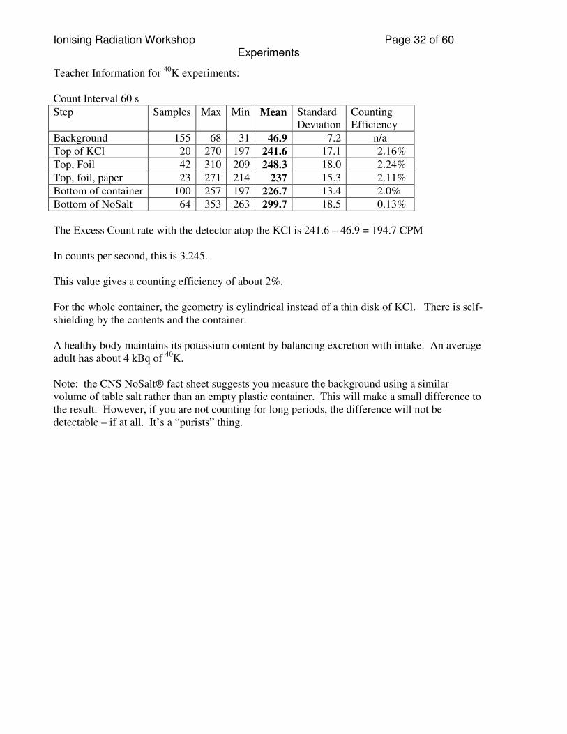
Ionising Radiation Workshop Page 32 of 60 Experiments
Teacher Information for 40K experiments: Count Interval 60 s
Step Samples Max Min Mean Standard Deviation
Counting Efficiency
Background 155 68 31 46.9 7.2 n/a
Top of KCl 20 270 197 241.6 17.1 2.16%
Top, Foil 42 310 209 248.3 18.0 2.24%
Top, foil, paper 23 271 214 237 15.3 2.11%
Bottom of container 100 257 197 226.7 13.4 2.0%
Bottom of NoSalt 64 353 263 299.7 18.5 0.13%
The Excess Count rate with the detector atop the KCl is 241.6 – 46.9 = 194.7 CPM In counts per second, this is 3.245. This value gives a counting efficiency of about 2%. For the whole container, the geometry is cylindrical instead of a thin disk of KCl. There is self-shielding by the contents and the container. A healthy body maintains its potassium content by balancing excretion with intake. An average adult has about 4 kBq of 40K. Note: the CNS NoSalt® fact sheet suggests you measure the background using a similar volume of table salt rather than an empty plastic container. This will make a small difference to the result. However, if you are not counting for long periods, the difference will not be detectable – if at all. It’s a “purists” thing.

Ionising Radiation Workshop Page 33 of 60 Experiments
Geiger Counter Experiment 3: Thorium-232
Reference: CNS publication “Naturally Occurring Radioactive Material fact sheet” Objective: In this experiment, the students will detect the ionising radiation emitted by an older consumer product available from eBay. With the use of absorbers, the students will be able to distinguish between alpha, beta and gamma radiation. Equipment:
1. RM-80 Geiger system as in Experiment 1 2. A vintage camera (see Appendix B) 3. Several circular disks of aluminum foil having a diameter slightly larger than the
diameter of the camera lens – not the outer bezel diameter. It may have a “tail” to make it easier to remove (with tweezers).
4. A few circular disks of paper similar to the aluminum foil disk above. 5. A ruler and / or a depth gauge. 6. Some cardboard or wooden spacers to help align the camera and detector/
Preparation: The system should be configured as described in Experiment 0. A counting interval (time base unit) of 10 or 20 seconds is recommended for measurements with these camera lenses. (See Experiment 0 Steps 5 & 7.) Count rates with these sources will exceed 5000 counts per minute! If the camera you are using has a removeable threaded insert in the front of the lens shroud, remove it to minimise the separation between the Geiger and the lens. If you have performed Experiment 1 with the same computer, you may skip steps: 4, 5, 6, and 8 below.
1. Click on the “Rad Collection” tab – click on the “Express Start …” command.
2. A window will open with the title “Select Aware Binary Rad Data File …” – click on “Cancel” unless you wish to use this function.
3. If the ASCII data file function is enabled, a window will open titled “Aware ASCII Output File …” If you do not wish to record data (to use in a spreadsheet or other program, click on “Cancel”. OR If you do wish to record data, the default location for the file is in the “C:\Aware” directory. You may select another directory. Enter a file name such as “camera.txt” (the “.txt” extension is not automatic). Click on the “Save” button. The program will start and will launch the running average bar graph in a separate

Ionising Radiation Workshop Page 34 of 60 Experiments
window.
4. Click on the Bar Graph window. Click on the “Options” tab. Here you may select either a “Points” average, or the “Alarm Average” value (default).
5. Click on the “Options” tab – click on the “Y value precision” function. A window will open. Select 0 as no decimal points are needed for the counts unit.
6. Click on the “Options” tab – click on the “Manual Y axis min” function. Ensure the value is zero.
7. Click on the “Options” tab – click on the “Manual Y axis max” function. Ensure the value is 1000 for camera lens measurements with a 10 s interval. By now, there should be a few bars on the graph. The auto function can be used, but it scales the graph to the highest value detected. This may result in the graph scale changing which can be confusing.
8. Click on the “Options” tab – ensure that the “Place spaces around numbers” function. This ensures the bars are spaced sufficiently widely that the count numbers are visible.
At this point you may click on the “Aw-Radw Exec #1” window and stop the data collection (Click on the “Rad Collection” tab – click on the “Stop Collection” function.) You may have to minimize the bar graph to find the control window. When you re-start data collection, your settings should be preserved. The program will ask you if you wish to record data files as in Steps 2 and 3 above. If you click on “Save” in step 3, the program will ask if you wish to over-write the data file you recorded previously. You may change the file name, or just click on “Yes”.

Ionising Radiation Workshop Page 35 of 60 Experiments
Procedure: Part I – Shielding Absorbers
1. Establish a background counting reference by letting the system collect data with the Camera kept well away from the Geiger. With a short counting interval of say 10 s, the average background number will be small (e.g. one-sixth of those measured previously). Record the average number of background counts in the interval.
2. Stand the camera on its base, and place the Geiger on its side, with the cable connector on the top. It will be necessary to raise the Geiger body by placing some spacers under it so it is not resting on the grey plastic bezel. This will make the Geiger axis horizontal. The camera may require spacers to raise the axis of the lens to be in line with the middle of the Geiger window. When this is done, the camera may be moved so that the camera lens shroud fits inside the Geiger bezel – moving the lens as close as possible to the Geiger window (touching its protective screen). Record the average number of counts in the interval.
3. Remove the camera and insert the paper disk in the in the lens shroud as close to the lens as possible. Return the camera to the same position as in step 2 and monitor the counting. Record the average number of counts in the interval.
4. Remove the camera, remove the paper disk and insert the aluminum foil disk in the lens shroud. Return the camera to the same position as in step 2 and monitor the counting. Record the average number of counts in the interval.
5. Remove the camera; insert the paper disk on top of the aluminum foil disk in the lens shroud. Return the camera to the same position as in step 2 and monitor the counting. Record the average number of counts in the interval.

Ionising Radiation Workshop Page 36 of 60 Experiments
Discussion of the Results
1. In each of the measurements made, the count rates with the camera present should be much larger than the background value. Background Count: _____________
2. With the camera lens close to the detector window, it will detect alpha, beta and gamma radiation. Counting time interval: __________ Sample Count: _____________
3. With the paper disk covering the lens, the number of alpha particles (and low-energy beta particles) detected by the Geiger will be significantly reduced. Sample Count with paper: __________________
4. With the foil disk covering the lens, the number of alpha particles reaching the detector will be very small. The foil will also reduce the number of beta particles. However, both the alpha and beta particles that scatter off atoms in the foil will produce a “shower” of low energy electrons that travel toward the detector. Sample Count with foil: ______________
5. With the foil disk followed by the paper disk, many of the “secondary” low energy electrons will be stopped. Sample Count with foil plus paper: _______________
6. In experiment 1, you estimated the counting efficiency of the detector for the beta and gamma emitted by 40K. If this counting efficiency is similar to that in step 3 (ignoring the alpha component), estimate the activity of the camera lens (beta, gamma). Activity = Sample Count with paper disk Counting Efficiency * Counting Interval Activity = ______________________________ Bq
Do you think the activity of the camera lens is larger or smaller than this value? _______ Why?

Ionising Radiation Workshop Page 37 of 60 Experiments
Teacher Information for Absorber Experiment:
Count interval: 10 s Position: minimum separation
Shield Samples Max Min Mean Std Dev
None 27 976 861 919.0 32.2
Paper 118 908 753 821.3 26.85
Foil 268 919 765 840.5 29.28
Foil + Paper 115 855 709 778.9 25.09
This data set shows that the introduction of a sheet of paper drops the count by 10.6%. Replacing the paper with foil produces a higher count rate! This is due to the alpha particles scattering electrons from the foil toward the detector.

Ionising Radiation Workshop Page 38 of 60 Experiments
Following the foil with a sheet of paper drops the count rate by 15.24% from the original measurement. The foil is stopping the majority of the alpha, some of the beta and a little of the gamma. Additional sheets of foil would lower the beta further. The number of counts for background with a 10 s interval is about 8 counts. Estimating the beta-gamma activity for the lens based on the paper shield count using 2% efficiency gives: 82.13 x 50 = 4 kBq The source may have more or less activity than this estimate. The factors include:
1. The lens area is much smaller than that of the layer of KCl measured previously. Hence the counting efficiency should be higher (not lower).
2. The lens is thicker than the thin disk layer of KCl – hence it will have more self-shielding for beta (and alpha). Moreover, the scattering geometry is much different than for the KCl. Net effect – who knows?
3. The paper shield will absorb some of the beta as well as the most of the alpha. A more extensive experiment was conducted with 20 s count intervals. The mean number of counts for each case is provided in the following table.
Number of Aluminum Foils (paper absorber is plotted as “0.1 foils”)
Case 0 0.1 1 2 3 4 5 6 7 8
No paper 1861 1748 1748 1733 1531 1470 1372 1349
Paper 1882 1686 1627 1569 1503 1424 1373 1328 1296 1267
The first data set was collected using aluminum foil absorbers in the lens shroud. The mean values are plotted. The plot points are scaled to appear about +/- 1 standard deviation, and are normalized to the (first) mean with no foil absorbers, only the air path (about 6.2 mm). The second data set was collected by introducing a paper absorber before the aluminum foils. The mean values are normalized to the mean for set 1. The results can be described as the alpha particles scattering electrons out of the first foil with higher energies than the beta or gamma that are coming out of the lens. While the alpha particle is positively charged, with its much higher energy and momentum it scatters an orbital electron from an atom – much like a soccer ball hitting a ping pong ball. The electrons don’t have a chance to bind to the alpha particle despite its positive charge. Some of the alpha particle energy and momentum is transferred to the atom that hosted the electron during the event. After some number of scattering events, the alpha particle slows sufficiently to acquire two electrons and behave like a helium gas atom.

Ionising Radiation Workshop Page 39 of 60 Experiments
Kodak Signet 40 Camera Lens, RM-80
2 data sets @ minimum separation without / with
paper absorber at lens (plotted as 0.1 foils)
60%
70%
80%
90%
100%
110%
0 1 2 3 4 5 6 7 8
# Al foil absorbers
Co
un
t N
orm
alized
re M
ean
for
Air
Path
(N
o A
bso
rbers
)
No Paper
Paper
These energetic electrons continue to scatter more electrons from successive foils, but the numbers and energies fall significantly after the 3rd foil as evidenced by the drop in the count rate with the 4th foil. When the paper absorber is introduced immediately after the lens, it drops the count rate by 10% and is assumed to have absorbed most of the alpha, some of the beta, and very little of the gamma radiation. The successive foils absorb more and more of the beta radiation (and some of the gamma radiation) until eventually the count rate is due largely to gamma radiation only. Why does the paper filter not produce scattered electrons in the foils?
Paper is made of hydrogen (1H), oxygen (16O), carbon (12C), and some other elements. It has low mass density (~0.8 kg/L), and provides a low density of electrons for the alpha particles to interact with. One sheet of ordinary copy paper (“20 lb”) has an area-density of 7.5 mg/cm2 and a thickness of about 90 µm. The alpha particles lose only a little energy with each scattering event, and are not stopped suddenly upon entering the sheet of paper. Aluminum is a metal (mass 27Al), and is much denser (2.7 kg/L) than paper. A typical aluminum foil sheet is thinner than a sheet of paper – about 19 µm thick and has an area-density of 5 mg/cm2. The alpha particles are stopped in a shorter distance in the foil. Moreover, the heavier atom binds some of its electrons much more strongly to the nucleus than do the lighter atoms. This changes the way energy is transferred to the electron, increasing the electron energy. The sheet of paper has an area density that is 50% greater than the aluminum foil, and is 4.5 times thicker. In shielding calculations the mass density is used as a proxy for the number of electrons. Shielding materials are described as providing “grams of mass per cm of thickness”. Using this rule, the electron density in the paper is about 3 times less than it is in the aluminum foil. Since the sheet of paper is 4.5 times thicker than the foil, the alpha particles travel further

Ionising Radiation Workshop Page 40 of 60 Experiments
in the paper than they do in the aluminum foil. With this experiment we don’t know if the alpha were just stopped in the full thickness of the sheet of paper – or were stopped half-way through. A thinner sheet of paper might produce a different result. Or not?
Why is the count rate after 1 foil greater than after 1 sheet of paper?
The single foil stops all the alpha particles, some of the beta and a little of the gamma radiation. However the alpha particle interactions in the foil scatter more electrons out of the foil than the number of alpha particles that are absorbed. Why is the count rate after 2 foils almost the same as after 1 foil?
The electrons scattered by the alpha particles from the 1st foil have sufficient energy to scatter enough electrons out of the 2nd and 3rd aluminum foils that the count rate changes very little. One sheet of paper absorbs the alpha particles without producing large numbers of higher energy electrons. The successive aluminum foils incrementally absorb the beta and gamma radiation, leading to successively lower count rates.

Ionising Radiation Workshop Page 41 of 60 Experiments
Procedure Part II – Range Measurements The camera lens source is sufficiently intense that it is possible to make measurements as a function of distance. Curriculum material may suggest that inverse square law spreading may be demonstrated. Alas, real experiment results are not quite that simple. The camera lens emits alpha, beta and gamma radiation. Both alpha and beta are absorbed in air much more strongly than gamma. To make the results simpler, it is suggested that a set of 4 absorbers be used to eliminate the alpha and reduce the beta content of the radiation:
• A paper absorber to reduce the alpha contribution
• 3 or more aluminum foils to reduce the beta (more is better, but the count rates will drop)
• A final paper absorber to reduce the low energy beta contribution.
1. In step 2 of Part I, you recorded the count rate at the minimum separation. To estimate this separation, measure the distance between the edge of the lens shroud and the face of the lens at its centre. Record this value.
2. Remove the shielding absorbers and reinsert as described above.
3. Use a piece of graph paper as a base so you can align the camera and Geiger – keeping them parallel. Place the camera HERE Mark the camera position. This will be your reference mark. Move the camera back to the next convenient grid line while taking care to keep it aligned with the Geiger detector axis. Mark the camera position on the graph paper. Record the average number of counts in the interval.
4. Move the camera back to the next convenient grid line. Mark the camera position on the graph paper. Record the average number of counts in the interval.
5. Repeat step 3 as many times as is convenient. Hint: it may be helpful to have more measurements at positions close to the Geiger, and increase the spacing as you move back. If your camera has a removable threaded insert for the lens shroud, re-installing it is a simple way to increase the separation by about 2 mm.

Ionising Radiation Workshop Page 42 of 60 Experiments
Discussion of the Results Complete the following Table
Step
Initial Measurement
[mm]
Distance from Reference Mark
[mm]
Sum of
Distances [mm]
Average Count in
Interval
1 0.00
2 3
4 5
6 7
8 9
10 Plot the data on a graph of Count versus Sum of Distances.

Ionising Radiation Workshop Page 43 of 60 Experiments
Teacher information on Range Experiment Kodak Signet 40 camera with lens shroud bezel removed, paper-3 foils-paper absorbers. Count Interval: 20 s
Step
Initial Measurement
[mm]
Distance from Reference Mark
[mm]
Sum of
Distances [mm]
Average Count in
Interval
1 6.6 0 6.6 1167
2 “ 2* 8.6 1080
3 “ 12 18.6 765
4 “ 22 28.6 546
5 “ 32 38.6 384
6 “ 42 48.6 289
7 “ 52 58.6 220
8 “ 62 68.6 179 * threaded insert re-installed.
Signet 40 Range Measurements
Absorbers: paper, 3 Al foils, paper
y = 0.284x2 - 36.637x + 1375.30
200
400
600
800
1000
1200
1400
1600
0 10 20 30 40 50 60 70
Lens to Geiger Distance [mm]
Co
un
ts p
er
20 s
in
terv
al
Count (20 s) 1/R-squared fit Poly. (Count (20 s))
The graph data shows that the count rate falls smoothly with distance. The dashed trend line fit is not a simple 1/R2. To accommodate the finite source size, the curve selected to fit the 5 points at greatest range values as:
( )6
21056.1
25
1××
+=
RY
does not represent the short range measurements. In addition to the finite size of the source of the radiation, the influence of residual beta as well as radiation scattered from the test jig complicate this measurement. 1/R2 is not easy to demonstrate!

Ionising Radiation Workshop Page 44 of 60 Appendices
Appendix A Access the CNS – 2008-2009
The Canadian Nuclear Society (CNS) provides Canadians interested in nuclear science and technology with a forum for technical and related discussion. The CNS endeavours to improve public knowledge in this area, through educational initiatives and by direct contact with CNS members. Many of our members are scientists and engineers working in the fields of nuclear science and technology. They comprise a valuable knowledge resource.
The following are three ways that you can access this resource:
1. CNS Education and Communication Committee
This committee exists to facilitate the exchange of information between CNS members and the public, and to develop educational programs in this regard. As a science educator, your input is important in ensuring that we allocated CNS resources where it is needed the most.
Contact: Dr. Jeremy Whitlock, email: [email protected], phone: 613-584-8811 AECL, Chalk River, Ontario, K0J 1J0 or Peter Lang CNS-ECC, email: [email protected], phone: 705-466-6136
2910 Concession 8, R.R. #1 Glen Huron, Ontario L0M 1L0 or Bryan White, email: [email protected], phone 613-584-4629 PO Box 1883, Deep River, Ontario, K0J 1P0 2. CNS Internet Website
The CNS is on the Web at www.cns-snc.ca. From here you can find information on national and local programs, and read more about the objectives of the Society. The website is administered by the Internet committee of the CNS. The CNS Office can be emailed at [email protected].
3. Local CNS Branches
There are fourteen local branches of the CNS, in five provinces. Each branch holds meetings with interesting speakers, and the public is welcome to attend. These branches may also receive a portion of the CNS Education Fund, to be administered locally (for science fair prizes, assistance in obtaining special equipment for high school science experiments, scholarships). In addition, each branch represents a local wealth of expertise that can be drawn upon for classroom presentations, participation in science fairs and other community events, or simply to answer questions. Listed below are the contact persons for each branch (usually the chairperson of the branch executive). Contact can also be made via our main website, given above.
Alberta Duane Pendergast 403 328-1804 [email protected]
Golden Horseshoe (Hamilton) Dave Novog 905-525-9140 x 24904 [email protected]
Pickering Marc Paiment 905-839-1151
Toronto Joshua Guin 905-728-8700
Bruce John Krane 519-361-4286
Manitoba Jason Martino 204-753-2311
Québec Michel Saint-Denis 514-875-3452
UOIT (Oshawa) Andrea Milner 905-436-7161
Chalk River Ragnar Dworschak 613-584-8811
New Brunswick Mark McIntyre 506-659-7636
Saskatchewan Walter Keyes 306-586-9536 [email protected]
Darlington Jacques Plourde 905-623-6670 x 7348
Ottawa Mike Taylor 613-692-1040
Sheridan Park (Mississauga) Peter Schwanke 905-823-9060

Ionising Radiation Workshop Page 45 of 60 Appendices
Appendix B Vintage Cameras / Lenses – thorium, a source to be reckoned with 1. Introduction Reference: www.orau.org/ptp/collection/consumer%20products/cameralens.htm From about 1950 through to 1980, several consumer cameras were produced using thorium oxide in the lens material to enhance the refractive index of the glass. Different recipes added from 12% to 28% of the glass as thorium oxide (under 30% was not regulated as a radioactive material.) The practice seems to have ended about 1980. (Other heavy metals such as lanthanum are used.) For high school demonstration experiments, these lenses are a conveniently “bright” source of particles. The radioactive material is embedded inside the glass of the lens, and most of the particle emissions are absorbed by air. There is no risk of radioactive contamination unless the lens is broken. There are occupational estimates of potential exposure based on such a lens being used as an eyepiece for 20 h per week that would result in surface exposure of 360 µSv to 8.8 mSv per year (this type of application was never approved). However, normal usage of a camera would result in exposures that rarely would exceed background levels. Using such “bright” sources that provide counting rates at or above 5000 counts per minute, many measurements can be made in a short time (accepting the statistical errors that result), and students are more likely to remain engaged in the process. Moreover, thorium-containing lenses are an interesting and useful source of alpha particles at very short distances. The following decay sequence shows that alpha, beta and gamma radiations are present and can be filtered out of the measured beam. Note that Bi-232 may follow either of 2 decay paths (~64% are β
- and ~36% α).
(figure from www.cameco.com)
Ionising Radiation Workshop Page 46 of 60 Appendices
2. Secular Equilibrium The term secular equilibrium refers to the activity of each of the radioactive decay products in a decay chain for long time scales relative to the half-lives involved. Thorium is a particularly interesting case since while Th-232 has a very long half-life, the balance of the decay products have very short half-lives, with the exception of Ra-228 and Th-228. When thorium is refined chemically for an application such as ThO2 content in glass lenses or refractory ceramics (very high temperature crucibles for example), the concentration of Ra-228 and the other non-thorium nuclides will be significantly reduced. Refined thorium has a much reduced radioactivity compared to thorium ore (most often a form of sand). Hence a new lens or crucible would have a low level of radioactivity when manufactured. Following the refinement step, the radionuclides in the decay chain would each start “growing-in”. Initially the decay chain following from Th-228 would quickly develop to match the Th-228 activity level. Within about 5 half-lives – 18 days, the Ra-224 activity would match that of the Th-228, and each of the subsequent steps having shorter half-lives would follow the Ra-224. Because the Th-228 half life is 1/3 of that of Ra-228, the Th-228 activity would slowly decline as there is very little Ra-228 to decay to Th-228. After 5 half-lives – 29 years, the Ra-228 activity level would develop to match that of Th-232. At this point, the whole chain approaches equilibrium. At secular equilibrium, each decay step in the chain has the same activity level. One Th-232 decay is associated with 1 decay of each subsequent radionuclide (except for the Bi-212 branches). Eight α particles and ten β- particles (with their associated gamma) are produced for every Th-232 decay. Since the Th-232 half life is long, the activity for its specific decay is low, but the full chain is 18 times greater. Consequently, the thorium decay chain in a camera lens manufactured in 1970 would be approaching equilibrium by the year 1999. (If you compare the thorium decay chain with those for uranium, the uranium chains require over 100 000 years to reach secular equilibrium following refining – see CNS Uranium Decay Fact Sheet.) 3. Monitoring Camera Lens Activity Experiment 2 describes making measurements of vintage camera lenses using absorbers, and distance in air. The alpha particles have a very short range in air – a few cm at most. To detect the alpha it is necessary to get the lens element as close to the Geiger window as is possible. The experiment describes shimming the detector and camera so that the lens bezel fits into the protective collar that surrounds the Geiger detector window.
It is not recommended that you remove the protective collar and screen.
The mica window is very delicate, and once broken, the Geiger is not repairable.
Counting measurements made with a variety of camera lenses are shown in the following graph. It should be noted that while the maximum count rate for a USB-connected Geiger appears to be

Ionising Radiation Workshop Page 47 of 60 Appendices
about 10 000 counts per minute, these have been found to produce a 10% lower count rate at 5000 counts per minute. Similarly, the maximum count rates observed with lenses to date is 25000 counts per minute, using a conventional serial port. Computer processor speed does not seem to be significant. However, the maximum count rate for this serial port arrangement has not been determined – hence it too may be missing counts and misrepresenting the actual activity level.
Vintage Camera Lens Activity Measurements
at minimal distance to Geiger detector
0 5000 10000 15000 20000 25000
Mamiya/Sekor 55 mm f1.4 lens - back
Praktica (Zeiss) 50 mm f1.8 - back
Praktica (Zeiss) 50 mm f1.8 - front
Super Takumar (Asahi) 55 mm f2.9 -back
Mamiya/Sekor 55 mm f1.8 lens - back
Mamiya/Sekor 55 mm f1.8 lens - back
Kodak Signet 40
Kodak Instamatic 804
Kodak Bantam Range Finder
gaf Anscomatic 726
Counts per minute
(background < 50 CPM)
Both the Signet 40 and the Bantam cameras have removable rings on the lens shroud that were removed to reduce the air gap by about 2 mm for these measurements. Some of the single lens reflex camera lenses were much more intensely radioactive at the back than at the front. There are two aspects to consider, lens diameter (or area), and the minimum air gap separating the lens from the Geiger window. These are graphed below.

Ionising Radiation Workshop Page 48 of 60 Appendices
Maximum Count Rate vs Lens Diameter
y = 0.4536x3.2056
0
5000
10000
15000
20000
25000
30000
10 15 20 25 30 35
Diameter [mm]
Maxim
um
Co
un
t R
ate
[C
PM
]
The activity should scale with the area of the lens, provided all the lenses have the same fractional content of thorium. However, the alpha particles are strongly attenuated in the air gap.
Maximum Count Rate vs Lens Distance to Geiger
y = -2217.7x + 22870
0
5000
10000
15000
20000
25000
30000
0 2 4 6 8 10 12
Distance [mm]
Maxim
um
Co
un
t R
ate
[C
PM
]
The plotted line is a linear fit. Because the lens diameter is not much smaller than the Geiger window, inverse square law reduction does not apply (the lens is definitely not a point source). By normalizing the maximum count rate by the lens area and plotting the result as a function of the lens to Geiger window air gap one obtains a better fit. While this may look impressive, one must remember that this is a mixed-mode radiation measurement. The alpha particles strongly absorbed with distance in air, while the beta is less so, and the gamma attenuate very little. A good fit to data analysis for the wrong physical arguments can be misleading.

Ionising Radiation Workshop Page 49 of 60 Appendices
Maximum Count Rate / Lens Area vs Lens Distance to Geiger
y = -0.132x2 - 0.0416x + 21.173
0
5
10
15
20
25
0 2 4 6 8 10 12
Distance [mm]
Max C
ou
nt
rate
/ a
rea
[CP
M/m
m/m
m]
4. Reducing Source Intensity To monitor the activity of the more intense lenses with a USB-connected Geiger detector, shielding in the form of a large diameter steel washer works well. Washers for a half-inch bolt (or smaller or larger) are available in hardware stores. These may be taped to the body of the lens with the hole centred.
4. Acquiring Cameras or Lenses Several manufacturers produced thorium-containing lenses. These lenses tend to have a brown tint due to “radiation damage” to the lens glass. Many of the vintage single lens reflex camera lenses remain popular and are consequently expensive. A dysfunctional lens (e.g. scratched, fungal

Ionising Radiation Workshop Page 50 of 60 Appendices
growth, broken aperture, damaged threads) has little value. These may be purchased on eBay or found in some retailers. A quality lens will regularly cost much more than $20 US apart from the occasional bargain. A lens may not necessarily be detectably radioactive, depending on its date of manufacture. The two lenses shown above have the same model number, but differing serial numbers. The Mamiya/Sekor 55 mm f1.8 lens with serial number 74653 is radioactive, while serial number 86250 is not. Somewhere in between these two, the lens glass recipe was changed. On close inspection one can see that the centre of the rear element in the newer lens is very close to the end face of the surrounding metal barrel.
Kodak manufactured 3 series of cameras that frequently are available at more reasonable costs. Of these, the Signet 40 uses 35 mm film and may fetch a premium price. While collectors seem to value these relatively useless range finder cameras, they often may be purchased for less than $10 US. The shipping and handling fees tend to dominate the purchase cost.

Ionising Radiation Workshop Page 51 of 60 Appendices
Appendix C Vintage Vaseline Glass – uranium as treasure While natural uranium may be available as a piece of ore from a mine, the surface of this material is often frail. The ore may break to release small pieces or dust. There are consumer products that include uranium such as the glazing of orange “Fiestaware” table settings made in a particular period. Another form is Vaseline glassware. Uranium compounds have been used to colour glass for many years. During the Great Depression coloured glass items were popular and a wide variety of Vaseline glassware items may be found in specialty stores or on eBay. The name “Vaseline” was attributed to the glass because of the green-yellow hue of the doped glass. The genuine item fluoresces under ultraviolet light. It is recommended that one purchase only items that are shown as fluorescing.
The photograph shows pieces of glass (cullets), marbles, and a “toothpick holder”. The latter provides count rates of about 1300 counts per minute at minimum separation to the RM-80 detector. While these are less intense sources of ionising radiation than the thorium-containing camera lenses, they may be of greater interest to some students. As in the case of the camera lenses, the alpha emitting radioactive material is contained within the glass. Vaseline glass or “depression era glass” was popular early in the 20th Century. More modern variants may be made using depleted uranium. In either case the chemical processing used to prepare the uranium for addition to the glass would have reduced the content of most of the uranium decay chains, leaving uranium-238, and uranium-235 as well as the decay product uranium-234 (both of the latter are reduced in depleted uranium). If the uranium-234 is reduced, the return to secular equilibrium would require in excess of 1 million years. For natural uranium, the decay of thorium-230 would require about 400,000 years to return to secular equilibrium.

Ionising Radiation Workshop Page 52 of 60 Appendices
Appendix D Connecting an Aware Geiger to a Computer The Aware Electronics RM-80 Geiger requires a SERIAL PORT connection to a Windows computer. This type of connection allows the Geiger electronics to interrupt the computer processor. The interrupt allows the program to respond promptly to each Geiger detection event. This photograph shows a serial port connector on the back of a vintage laptop computer. The door is opened to access the connector. Many modern computers do not include serial ports.
• One may be added to a desktop computer by installing a special interface card.
• Older laptops may have a “PCIA” slot that will accept a serial port interface.
• For modern laptops, one may use a USB port to connect a serial port module. The photograph below shows a laptop with a PCIA slot Serial Port Interface card (the card is not fully inserted into the computer for visual effect). The BEIGE-coloured module mates the 4-wire telephone jack cable that plugs into the Geiger module with the Serial Port connector. (Note that newer “non-divide-by-two” are also red in colour.) The small black cable can be disconnected from the PCIA Serial Port Interface card so that the card may be left in the computer. DO NOT connect the telephone cable to a “modem” dial-up connection on the computer. This will not work!

Ionising Radiation Workshop Page 53 of 60 Appendices
The photograph below shows the Aware Geiger connected to a computer USB port using a USB Serial Port adapter. This adapter connects to the computer via a USB extension cable (black). The USB Serial Port adapter housing has a chunky shape that will not plug directly into many computer USB ports. The RED-coloured module mates the 4-wire telephone jack to the serial port connector on the adapter. This module includes a “Divide by 2” circuit, which is necessary to produce the correct number of processor interrupts for counting. (If you use a Beige module with a USB Serial Port adapter, the count rate will be doubled. If you use a Red ÷ by 2 module with a conventional / PCIA serial port, the count rate will be halved.)

Ionising Radiation Workshop Page 54 of 60 Appendices
Note: The Aware Electronics software does not require a high performance computer. An old desktop or laptop computer that includes a serial port may be a great low cost option. Limitations of the USB Interface The operation of the USB interface is not ideal for counting Geiger event pulses. At low count rates it performs very well. As the count rate increases, this type of interface will miss counting events and produce a lower average (and maximum) number of counts than a conventional serial port interface. Aware Electronics have offer an alternative USB-MSP product. Trials with a camera lens show that at about 5000 counts per minute, the USB interface produces about 10% fewer counts than a conventional serial port. The graph below shows such a comparison. The number of counts in each minute was analysed in terms of a frequency distribution (a histogram, similar to a bell curve for student marks). The smooth curves are reference normal distributions having the same means and standard deviations as the count data.
Kodak Signet 40 with Ektanon 46 mm f3.5 lens
bezel removed from front of lens
0%2%4%6%8%
10%12%14%16%18%20%
4600 4800 5000 5200 5400 5600 5800
CPM
Fre
qu
en
cy
Signet 40 sn 8809, pcia, no bezel, aligned reference normal
USB serial interface USB reference normal
USB Serial Interface Driver Installation The USB serial interface device is a “PL2303”. There is a set of driver installation files on the CD provided by the CNS, or the micro-CD enclosed with the USB interface. Select and run the appropriate file for your system before connecting the USB interface. Note that if you use a different USB port, you will end up with an additional installation, and another “COM” port. If possible, use the same USB port each time to avoid confusion.

Ionising Radiation Workshop Page 55 of 60 Appendices
Microsoft Vista® Computers The Aware Electronics website advises that their Aw-Radw program is compatible with Vista. The USB serial port interface (PL-2303) manufacturer does not supply a Vista-compatible driver. These are available from websites such as: www.cooldrives.com/wividrforprc.html. The CNS has tested this configuration with Vista® Premium Business. Aware Electronics Software Installation The Aware Electronics manual includes installation instructions. The following summary should cover most needs.
1. Create a folder (directory) C:\Aware 2. Copy the contents of the Aware software directory on the CD to that folder 3. Select the Aw-Radw icon / executable program, right click and then click on create a
shortcut 4. Select the shortcut and drag it to the desktop
Ionising Radiation Workshop Page 56 of 60 Appendices
Appendix E Units of Radiation Measurements Reference: http://www.hc-sc.gc.ca/ed-ud/event-incident/radiolog/info/measure-mesure-eng.php The units of radiation measurement used in Canada and in much of the world are Système Internationale (SI) units, based on the metric system. These units include the �utherfor, the gray, and the sievert, terms which are described below. In the 1960’s the SI units of radiation replaced another set of units, which had been in use from the early twentieth century. The older units are still used in the United States and are found in some earlier documents; they are summarised in the table below. Bequerel
The �utherfor (Bq) is the unit used to measure radioactivity in a substance, without consideration for the type of radiation it is or what its effects may be. One �utherfor is equal to one nuclear disintegration per second. Since this is a very small unit, other units are often used, including the kilobecquerel (kBq: thousand Bq), megabecquerel (MBq: million Bq), and gigabecquerel (GBq: thousand million Bq). The name recognises the scientific contributions of French physicist A-H. Becquerel. Gray
The gray (Gy) is the unit used in describing the amount of energy absorbed by a substance from the radiation passing through it, or the (absorbed) dose. One gray corresponds to one joule of radiation energy absorbed by one kilogram of matter. The measurement of grays per hour received by a substance tells us the intensity of the radiation. This unit was named after the English radiobiologist Louis H. Gray. Sievert
The sievert (Sv) is the unit that reflects the biological effects of the ionising radiation absorbed; it is used in expressing both the equivalent dose and the effective dose. The sievert is a very large dose of radiation; a more useful unit is the millisievert (mSv), which is one-thousandth of a sievert. The name honours Rolf M. Sievert, a Swedish physicist. Person-sievert
The person-sievert (person-Sv) is the unit used to express the collective dose, a useful measure of the total radiation exposure resulting from a specific source or activity to an entire group of people.
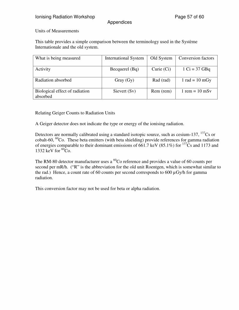
Ionising Radiation Workshop Page 57 of 60 Appendices
Units of Measurements This table provides a simple comparison between the terminology used in the Système Internationale and the old system.
What is being measured
International System
Old System
Conversion factors
Activity
Becquerel (Bq)
Curie (Ci)
1 Ci = 37 GBq
Radiation absorbed
Gray (Gy) Rad (rad)
1 rad = 10 mGy
Biological effect of radiation absorbed
Sievert (Sv)
Rem (rem)
1 rem = 10 mSv
Relating Geiger Counts to Radiation Units A Geiger detector does not indicate the type or energy of the ionising radiation. Detectors are normally calibrated using a standard isotopic source, such as cesium-137, 137Cs or cobalt-60, 60Co. These beta emitters (with beta shielding) provide references for gamma radiation of energies comparable to their dominant emissions of 661.7 keV (85.1%) for 137Cs and 1173 and 1332 keV for 60Co. The RM-80 detector manufacturer uses a 60Co reference and provides a value of 60 counts per second per mR/h. (“R” is the abbreviation for the old unit Roentgen, which is somewhat similar to the rad.) Hence, a count rate of 60 counts per second corresponds to 600 µGy/h for gamma radiation. This conversion factor may not be used for beta or alpha radiation.

Canadian Nuclear Society / Société Nuclaire Canadienne Ionising Radiation Workshop
Appendix F: Recommended Links for Educators and Students 2009-11-21 Page 58 of 60 Subject (alphabetical)
Organization Website
AECL, CANDU Reactors Atomic Energy of Canada Ltd. www.aecl.ca AECL, Education Atomic Energy of Canada Ltd. www.aecl.ca/Resources.htm Canadian Nuclear FAQ Dr. Jeremy Whitlock www.nuclearfaq.ca/ Canadian Nuclear Industry Canadian Nuclear Association www.cna.ca Canadian Research Reactors
Atomic Energy of Canada Ltd. history CBC Archives ZEEP NRU Algonquin College McMaster Nuclear Reactor Slowpoke University of Alberta Dalhousie University École Polytechnique Saskatchewan Research Council
www.aecl.ca/Science/RR/History.htm archives.cbc.ca/science_technology/energy_production/clips/893/ http://www.cns-snc.ca/history/ZEEP/ZEEP_AECL1970.pdf www.aecl.ca/Science/CRL/NRU.htm www.nrucanada.ca/en/default.htm www.nrureactor.ca www.science.mcmaster.ca/mnr/Main-Page/Frameset-homepage.htm mnr.mcmaster.ca www.ualberta.ca/~slowpoke/ environmentalhealthandsafetyoffice.dal.ca/slowpoke.htm www.polymtl.ca/nucleaire/en/LTN/SLP.php www.src.sk.ca/html/labs_facilities/analytical_labs/index.cfm
Canadian Utility Bruce Power www.brucepower.com/pagecontent.aspx?navuid=1 Canadian Utility Hydro-Québec www.hydroquebec.com/generation/classics/nuclear/gentilly_2/index.html Canadian Utility New Brunswick Power
Pt. Lepreau Refurbishment nbpower.com/html/en/about/operating/nuclear.html poweringthefuture.nbpower.com/en/Default.asp
Canadian Utility Ontario Power Generation www.opg.com/index.asp CNA Education Canadian Nuclear Association www.cna.ca/curriculum/default.asp CNS Education Page Canadian Nuclear Society www.cns-snc.ca/ecc/cnsecc.html Education / Radiation CBC Radio archives, Montreal Laboratory 1945
Yes I Can Science Electromagnetic Radiation Measuring Radiation – EVARMS
Ionising Radiation Unit
archives.cbc.ca/science_technology/energy_production/clips/889/ resources.yesican-science.ca/trek/radiation/final/index_em_matter.html resources.yesican-science.ca/trek/radiation/final/index_EVARMS.html radarsat.space.gc.ca/eng/educators/resources/evarm/grade11/measuring.asp resources.yesican-science.ca/trek/radiation/final/index.html
Energy Supply Nobody’s Fuel www.nobodysfuel.com/intro.html Energy Units Digg, spiral of energy scale – 100 orders of magnitude i206.photobucket.com/albums/bb127/drenka2busy/Nerdy stuff/energy-
scale-100-orders-of-magnitud.jpg Geiger detectors, software Aware Electronics Corporation www.aw-el.com/ Geiger detectors, software Black Cat Systems www.blackcatsystems.com/GM/GeigerCounters.html Geiger tubes LND Inc. www.lndinc.com/ Industrial Radioisotopes World Nuclear Association www.world-nuclear.org/info/inf56.html Interactive Chart of the National Nuclear Data Centre, Brookhaven National www.nndc.bnl.gov/chart/

Canadian Nuclear Society / Société Nuclaire Canadienne Ionising Radiation Workshop
Appendix F: Recommended Links for Educators and Students 2009-11-21 Page 59 of 60 Subject (alphabetical)
Organization Website
Nuclides Laboratory International Nuclear Industry
International Atomic Energy Agency World Nuclear Association (photos) Power Plants Around the World World Association of Nuclear Operators Uranium Institute (Australia)
www.iaea.org/ www.world-nuclear.org/ www.industcards.com/ppworld.htm#fuel%20cell%20power%20plants www.wano.org.uk/ uic.com.au/
Ionising and Non-ionising Radiation
US EPA www.epa.gov/rpdweb00/understand/ionize_nonionize.html
Lord Ernest Rutherford Museum
Professor John Campbell (biographer) McGill University
www.rutherford.org.nz www.physics.mcgill.ca/museum/�utherford_museum.htm
Medical Radioisotopes MDS Nordion World Nuclear Association
www.mds.nordion.com www.world-nuclear.org/info/inf55.html
Neutrinos
Geoneutrinos
Laboratoire d’Annecy-le-Vieux de Physique des Particules, CEDEX France University of Illinois at Urbana, Astronomy Dept.
www.lapp.in2p3.fr/neutrinos/anhistory.html www.astro.uiuc.edu/~bdfields/geoneutrinos.html
Neutrinos – SNO Lab Queen’s University www.sno.phy.queensu.ca/ Neutron Scattering National Research Council
Canadian Neutron Beam Centre neutron.nrc-cnrc.gc.ca/home_e.html
Nuclear Wall Chart Lawrence Livermore Laboratories www.lbl.gov/abc/wallchart/guide.html NORM Transportation Health Canada www.hc-sc.gc.ca/ewh-semt/pubs/contaminants/norm-mrn/index-eng.php Periodic Table Radiochemistry Society www.radiochemistry.org/periodictable/index.shtml Periodic Table – song Tom Lehrer’s Elements song animated with table
words
http://www.youtube.com/watch?v=SmwlzwGMMwc http://www.youtube.com/watch?v=GFIvXVMbII0 http://video.google.ca/videoplay?docid=-7098049931934196791&ei=YrLTSdeoCoqW_AGzvZGFCg&q=tom+�ehrer+site+elements+song
Physics Demos CNS Mousetrap & Superball Chain Reaction www.cns-snc.ca/ecc/cns_chain_reaction.wmv Physics Demos St. Mary’s University including mousetrap reactor www.ap.smu.ca/demos/navigation/navigation_frames.html Physics Demos Ithaca Science Center Mousetrap Cascade www.youtube.com/watch?v=XHitaEy-Xtg Planck’s Constant Perimeter Institute high school experiment www.perimeterinstitute.ca/en/Outreach/Plancks_Constant/Measuring_Pla
nck’s_Constant%3A_Introduction/ Particle Decay Berkley Lab The Particle Adventure www.particleadventure.org/decay_intro.html

Canadian Nuclear Society / Société Nuclaire Canadienne Ionising Radiation Workshop
Appendix F: Recommended Links for Educators and Students 2009-11-21 Page 60 of 60 Radiation & Radioactivity
Consumer Products
Wilhelm Roentgen Radiation effects NORM
Natural Reactors – Oklo Terrestrial Radiation
Canadian Nuclear Association US Government Health Physics Society Oak Ridge Area Universities Resonance Publications UN – Scientific Committee Effects Atomic Radiation Idaho State University Curtin University of Technology, Australia Twin Health Group, Japan ?
www.cna.ca/english/facts.asp www.epa.gov/rpdweb00/understand/index.html www.hps.org/ www.orau.org/ptp/collection/consumer%20products/consumer.htm www.resonancepub.com/wroentgen.htm www.unscear.org/unscear/en/publications.html www.physics.isu.edu/radinf/natural.htm www.oklo.curtin.edu.au/ www.taishitsu.or.jp/radiation/index-e.html
Radiation Epidemiology National Council on Radiation Protection & Measurements
http://www.ncrponline.org/PDFs/Boice.pdf
Radiation Geophysics Geological Survey of Canada gsc.nrcan.gc.ca/gamma/dist/index_e.php Radon
Home Owners Health Canada & Canada Mortgage & Housing Corporation
www.hc-sc.gc.ca/hl-vs/iyh-vsv/environ/radon-eng.php www.cmhc-schl.gc.ca/odpub/pdf/61945.pdf
Safety Canadian Nuclear Safety Commission www.nuclearsafety.gc.ca/eng/ Science Workbooks, lesson plans, Australian context
Australian Nuclear Science and Technology Org.
www.ansto.gov.au/education_resources
The Standard Model Lawrence Berkeley National Laboratory www.particleadventure.org/decay_intro.html Sticky Tape Gamma Physics Dept., UCLA video http://www.nature.com/nature/videoarchive/x-rays/ Uranium
In drinking water Cameco Corp. Educational Material Canadian Medical Association Journal
www.cameco.com/uranium_101/ www.cmaj.ca/cgi/content/full/170/6/951
US Nuclear Industry Whatisnuclear.com www.whatisnuclear.com/ Vaseline Glass Oak Ridge Area Universities www.orau.org/ptp/collection/consumer products/vaseline.htm