Embed Size (px)
Citation preview
Physics Reports 412 (2005) 1 – 88www.elsevier.com/locate/physrep
BCS–BEC crossover: From high temperature superconductorsto ultracold superfluids
Qijin Chena,1, Jelena Stajicb,2, Shina Tanb, K. Levinb,∗
aDepartment of Physics and Astronomy, Johns Hopkins University, Baltimore, MD 21218, USAbJames Franck Institute and Department of Physics, University of Chicago, Chicago, IL 60637, USA
Accepted 15 February 2005
editor: D.L. Mills
Abstract
We review the BCS to Bose–Einstein condensation (BEC) crossover scenario which is based on the well knowncrossover generalization of the BCS ground state wavefunction 0. While this ground state has been summarizedextensively in the literature, this Review is devoted to less widely discussed issues: understanding the effects offinite temperature, primarily below Tc, in a manner consistent with 0. Our emphasis is on the intersection of twoimportant problems: highTc superconductivity and superfluidity in ultracold fermionic atomic gases. We address the“pseudogap state” in the copper oxide superconductors from the vantage point of a BCS–BEC crossover scenario,although there is no consensus on the applicability of this scheme to highTc. We argue that it also provides a usefulbasis for studying atomic gases near the unitary scattering regime; they are most likely in the counterpart pseudogapphase. That is, superconductivity takes place out of a non-Fermi liquid state where preformed, metastable fermionpairs are present at the onset of their Bose condensation. As a microscopic basis for this work, we summarizea variety of T-matrix approaches, and assess their theoretical consistency. A close connection with conventionalsuperconducting fluctuation theories is emphasized and exploited.© 2005 Elsevier B.V. All rights reserved.
PACS: 03.75.−b; 74.20.−z
Keywords: Bose–Einstein condensation; BCS–BEC crossover; Fermionic superfluidity; HighTc superconductivity
∗Corresponding author.E-mail address: [email protected] (K. Levin).
1 Current address: James Franck Institute and Department of Physics, University of Chicago, Chicago, IL 60637, USA.2 Current address: Los Alamos National Laboratory, Los Alamos, NM 87545, USA.
0370-1573/$ - see front matter © 2005 Elsevier B.V. All rights reserved.doi:10.1016/j.physrep.2005.02.005
2 Q. Chen et al. / Physics Reports 412 (2005) 1 – 88
Contents
1. Introduction to qualitative crossover picture . . . . . . . . . . . . . . . . . . . . . . . . . . . . . . . . . . . . . . . . . . . . . . . . . . . . . . . . . . . . . . . .31.1. Fermionic pseudogaps and meta-stable pairs: two sides of the same coin . . . . . . . . . . . . . . . . . . . . . . . . . . . . . . . . . .41.2. Introduction to high Tc superconductivity: pseudogap effects . . . . . . . . . . . . . . . . . . . . . . . . . . . . . . . . . . . . . . . . . . . .81.3. Introduction to high Tc superconductivity: Mott physics and possible ordered states . . . . . . . . . . . . . . . . . . . . . . . . .151.4. Overview of the BCS–BEC picture of highTc superconductors in the underdoped regime . . . . . . . . . . . . . . . . . . . .17
1.4.1. Searching for the definitive highTc theory . . . . . . . . . . . . . . . . . . . . . . . . . . . . . . . . . . . . . . . . . . . . . . . . . .191.5. Many body Hamiltonian and two body scattering theory: mostly cold atoms . . . . . . . . . . . . . . . . . . . . . . . . . . . . . . .20
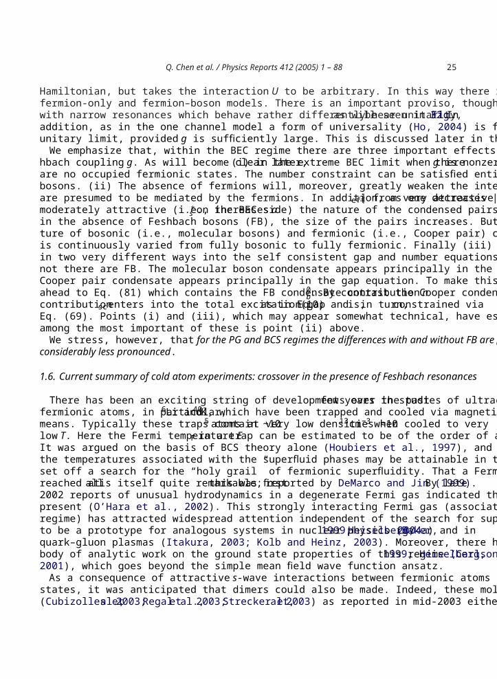
1.5.1. Differences between one and two channel models: physics of Feshbach bosons . . . . . . . . . . . . . . . . . . .241.6. Current summary of cold atom experiments: crossover in the presence of Feshbach resonances . . . . . . . . . . . . . . . 251.7. T-matrix-based approaches to BCS–BEC crossover in the absence of Feshbach effects . . . . . . . . . . . . . . . . . . . . . .28
1.7.1. Review of BCS theory using the T-matrix approach . . . . . . . . . . . . . . . . . . . . . . . . . . . . . . . . . . . . . . . . . .291.7.2. Three choices for the T-matrix of the normal state: problems with the Nozieres Schmitt-Rink approach 30
1.8. Superconducting fluctuations: a type of pre-formed pairs . . . . . . . . . . . . . . . . . . . . . . . . . . . . . . . . . . . . . . . . . . . . . . .321.8.1. Dynamics of pre-formed pairs aboveTc: time dependent Ginzburg–Landau theory . . . . . . . . . . . . . . . . 33
2. Quantitative details of crossover . . . . . . . . . . . . . . . . . . . . . . . . . . . . . . . . . . . . . . . . . . . . . . . . . . . . . . . . . . . . . . . . . . . . . . . . .352.1. T = 0, BEC limit without Feshbach bosons . . . . . . . . . . . . . . . . . . . . . . . . . . . . . . . . . . . . . . . . . . . . . . . . . . . . . . . . . .352.2. Extending conventional crossover ground state toT = 0: BEC limit without Feshbach bosons . . . . . . . . . . . . . . . .372.3. Extending conventional crossover ground state toT = 0: T-matrix scheme in the presence of Feshbach bosons . . 382.4. Nature of the pair dispersion: size and lifetime of noncondensed pairs belowTc . . . . . . . . . . . . . . . . . . . . . . . . . . . .422.5. Tc calculations: analytics and numerics . . . . . . . . . . . . . . . . . . . . . . . . . . . . . . . . . . . . . . . . . . . . . . . . . . . . . . . . . . . . . .43
3. Self consistency tests . . . . . . . . . . . . . . . . . . . . . . . . . . . . . . . . . . . . . . . . . . . . . . . . . . . . . . . . . . . . . . . . . . . . . . . . . . . . . . . . . . .443.1. Important check: behavior of s . . . . . . . . . . . . . . . . . . . . . . . . . . . . . . . . . . . . . . . . . . . . . . . . . . . . . . . . . . . . . . . . . . . .453.2. Collective modes and gauge invariance . . . . . . . . . . . . . . . . . . . . . . . . . . . . . . . . . . . . . . . . . . . . . . . . . . . . . . . . . . . . . .463.3. Investigating the applicability of a Nambu matrix Green’s function formulation . . . . . . . . . . . . . . . . . . . . . . . . . . . .49
4. Other theoretical approaches to the crossover problem . . . . . . . . . . . . . . . . . . . . . . . . . . . . . . . . . . . . . . . . . . . . . . . . . . . . . . .504.1. T = 0 theories . . . . . . . . . . . . . . . . . . . . . . . . . . . . . . . . . . . . . . . . . . . . . . . . . . . . . . . . . . . . . . . . . . . . . . . . . . . . . . . . . . .504.2. Boson–Fermion models for highTc superconductors . . . . . . . . . . . . . . . . . . . . . . . . . . . . . . . . . . . . . . . . . . . . . . . . . . .52
5. Physical implications: ultracold atom superfluidity . . . . . . . . . . . . . . . . . . . . . . . . . . . . . . . . . . . . . . . . . . . . . . . . . . . . . . . . . .525.1. Homogeneous case . . . . . . . . . . . . . . . . . . . . . . . . . . . . . . . . . . . . . . . . . . . . . . . . . . . . . . . . . . . . . . . . . . . . . . . . . . . . . . .52
5.1.1. Unitary limit and universality . . . . . . . . . . . . . . . . . . . . . . . . . . . . . . . . . . . . . . . . . . . . . . . . . . . . . . . . . . . . .575.1.2. Weak Feshbach resonance regime:|g0| =0+ . . . . . . . . . . . . . . . . . . . . . . . . . . . . . . . . . . . . . . . . . . . . . . . .60
5.2. Superfluidity in traps . . . . . . . . . . . . . . . . . . . . . . . . . . . . . . . . . . . . . . . . . . . . . . . . . . . . . . . . . . . . . . . . . . . . . . . . . . . . .615.3. Comparison between theory and experiment: cold atoms . . . . . . . . . . . . . . . . . . . . . . . . . . . . . . . . . . . . . . . . . . . . . . . .64
6. Physical implications: high Tc superconductivity . . . . . . . . . . . . . . . . . . . . . . . . . . . . . . . . . . . . . . . . . . . . . . . . . . . . . . . . . . .656.1. Phase diagram and superconductor–insulator transition: boson localization effects . . . . . . . . . . . . . . . . . . . . . . . . . .656.2. Superconducting coherence effects . . . . . . . . . . . . . . . . . . . . . . . . . . . . . . . . . . . . . . . . . . . . . . . . . . . . . . . . . . . . . . . . . .666.3. Electrodynamics and thermal conductivity . . . . . . . . . . . . . . . . . . . . . . . . . . . . . . . . . . . . . . . . . . . . . . . . . . . . . . . . . . .696.4. Thermodynamics and pair-breaking effects . . . . . . . . . . . . . . . . . . . . . . . . . . . . . . . . . . . . . . . . . . . . . . . . . . . . . . . . . . .726.5. Anomalous normal state transport: Nernst and other precursor transport contributions . . . . . . . . . . . . . . . . . . . . . . .72
6.5.1. Quantum extension of TDGL . . . . . . . . . . . . . . . . . . . . . . . . . . . . . . . . . . . . . . . . . . . . . . . . . . . . . . . . . . . . .736.5.2. Comparison with transport data . . . . . . . . . . . . . . . . . . . . . . . . . . . . . . . . . . . . . . . . . . . . . . . . . . . . . . . . . . .74
7. Conclusions . . . . . . . . . . . . . . . . . . . . . . . . . . . . . . . . . . . . . . . . . . . . . . . . . . . . . . . . . . . . . . . . . . . . . . . . . . . . . . . . . . . . . . . . . .76Acknowledgements . . . . . . . . . . . . . . . . . . . . . . . . . . . . . . . . . . . . . . . . . . . . . . . . . . . . . . . . . . . . . . . . . . . . . . . . . . . . . . . . . . . . . . .77Appendix A. Derivation of theT = 0 variational conditions . . . . . . . . . . . . . . . . . . . . . . . . . . . . . . . . . . . . . . . . . . . . . . . . . . . . .77Appendix B. Proof of Ward identity belowTc . . . . . . . . . . . . . . . . . . . . . . . . . . . . . . . . . . . . . . . . . . . . . . . . . . . . . . . . . . . . . . . . .78Appendix C. Quantitative relation between BCS–BEC crossover and Hartree-TDGL . . . . . . . . . . . . . . . . . . . . . . . . . . . . . . . .80Appendix D. Convention and notation . . . . . . . . . . . . . . . . . . . . . . . . . . . . . . . . . . . . . . . . . . . . . . . . . . . . . . . . . . . . . . . . . . . . . . .82
D.1. Notation . . . . . . . . . . . . . . . . . . . . . . . . . . . . . . . . . . . . . . . . . . . . . . . . . . . . . . . . . . . . . . . . . . . . . . . . . . . . . . . . . . . . . . . .82D.2. Convention for units . . . . . . . . . . . . . . . . . . . . . . . . . . . . . . . . . . . . . . . . . . . . . . . . . . . . . . . . . . . . . . . . . . . . . . . . . . . . . .83
Q. Chen et al. / Physics Reports 412 (2005) 1 – 88 3
D.3. Abbreviations . . . . . . . . . . . . . . . . . . . . . . . . . . . . . . . . . . . . . . . . . . . . . . . . . . . . . . . . . . . . . . . . . . . . . . . . . . . . . . . . . . . .83References . . . . . . . . . . . . . . . . . . . . . . . . . . . . . . . . . . . . . . . . . . . . . . . . . . . . . . . . . . . . . . . . . . . . . . . . . . . . . . . . . . . . . . . . . . . . . .84
1. Introduction to qualitative crossover picture
This review addresses an extended form of the BCS theory of superfluidity (or superconductivity) knownas “BCS–Bose–Einstein condensation (BEC) crossover theory”. Here we contemplate a generalization ofthe standard mean field description of superfluids now modified so that one allows attractive interactionsof arbitrary strength. In this way one describes how the system smoothly goes from being a superfluidsystem of the BCS type (where the attraction is arbitrarily weak) to a Bose Einstein condensate of diatomicmolecules (where the attraction is arbitrarily strong). One, thereby, sees that BCS theory is intimatelyconnected to BEC. Attractive interactions between fermions are needed to form “bosonic-like” molecules(called Cooper pairs) which then are driven statistically to Bose condense. BCS theory is a special casein which the condensation and pair formation temperatures coincide.
The importance of obtaining a generalization of BCS theory which addresses the crossover from BCS toBEC at general temperatures T ⩽Tc cannot be overestimated. BCS theory as originally postulated can beviewed as a paradigm among theories of condensed matter systems; it is complete, in many ways genericand model independent, and well verified experimentally. The observation that a BCS-like approachgoes beyond strict BCS theory, suggests that there is a larger mean field theory to be addressed. Equallyexciting is the possibility that this mean field theory can be discovered and simultaneously tested in a verycontrolled fashion using ultracold fermionic atoms. We presume here that it may also have applicabilityto other short coherence length materials, such as the high temperature superconductors.
This Review is written in order to convey important new developments from one subfield of physics toanother. Here it is hoped that we will communicate the recent excitement felt by the cold atom communityto condensed matter physicists. Conversely we wish to communicate a comparable excitement in studies ofhigh temperature superconductivity to atomic physicists. There has been a revolution in our understandingof ultracold fermions in traps in the last few years. The milestones in this research were the creation ofa degenerate Fermi gas (1999), the formation of dimers of fermions (2003), Bose-Einstein condensation(BEC) of these dimers (late 2003) and finally superfluidity of fermionic pairs (2004).
In high temperature superconductors the BCS–BEC crossover picture has been investigated for manyyears now. It leads to a particular interpretation of a fascinating, but not well understood phase, known asthe “pseudogap state”. In the cold atom system, this crossover description is not just a scenario, but hasbeen realized in the laboratory. This is because one has the ability (via Feshbach resonances) to applymagnetic fields in a controlled way to tune the strength of the attraction. We note, finally, that researchin this field has not been limited exclusively to the two communities. One has seen the application ofthese crossover ideas to studies of excitons in solids (Lai et al., 2004), to nuclear physics (Baldo et al.,1995; Heiselberg, 2004a) and to particle physics (Itakura, 2003; Klinkhamer and Volovik, 2004; Kolband Heinz, 2003) as well. There are not many problems in physics which have as great an overlap withdifferent subfield communities as this “BCS–BEC crossover problem”.
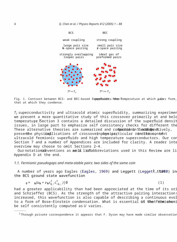
In this Review, we begin with an introduction to the qualitative picture of the BCS–BEC crossoverscenario which is represented schematically in Fig. 1. We discuss this picture in the context of both high
4 Q. Chen et al. / Physics Reports 412 (2005) 1 – 88
BCS BEC
weak coupling strong coupling
large pair size small pair sizek-space pairing r-space pairing
strongly overlapping ideal gas ofCooper pairs preformed pairs
T* = Tc T* >> Tc
Fig. 1. Contrast between BCS- and BEC-based superfluids. HereT∗represents the temperature at which pairs form, whileTc isthat at which they condense.
Tc superconductivity and ultracold atomic superfluidity, summarizing experiments in both. In Section 2,we present a more quantitative study of this crossover primarily at and below the superfluid transitiontemperature Tc. Section 3 contains a detailed discussion of the superfluid density and gauge invarianceissues, in large part to emphasize self consistency checks for different theoretical approaches to crossover.These alternative theories are summarized and compared in Section 4. Sections 5 and 6, respectively,present the physical implications of crossover physics, in one particular rendition, in the context ofultracold fermionic superfluids and high temperature superconductors. Our conclusions are presented inSection 7 and a number of Appendices are included for clarity. A reader interested in only the broadoverview may choose to omit Sections 2–4.
Our notational conventions as well as a list of abbreviations used in this Review are listed inAppendix D at the end.
1.1. Fermionic pseudogaps and meta-stable pairs: two sides of the same coin
A number of years ago Eagles (Eagles, 1969) and Leggett (Leggett, 1980) independently noted1 thatthe BCS ground state wavefunction
0 = k(uk + vkc†k,↑c†
−k,↓)|0 (1)
had a greater applicability than had been appreciated at the time of its original proposal by Bardeen, Cooperand Schrieffer (BCS). As the strength of the attractive pairing interaction U ( <0) between fermions isincreased, this wavefunction is also capable of describing a continuous evolution from BCS like behaviorto a form of Bose–Einstein condensation. What is essential is that the chemical potential of the fermionsbe self consistently computed as U varies.
1 Through private correspondence it appears that F. Dyson may have made similar observations even earlier.
Q. Chen et al. / Physics Reports 412 (2005) 1 – 88 5
The variational parameters vk and uk which appear in Eq. (1) are usually represented by the two moredirectly accessible parameters sc(0) and , which characterize the fermionic system. Here sc(0) is thezero temperature superconducting order parameter. These fermionic parameters are uniquely determinedin terms of U and the fermionic density n. The variationally determined self consistency conditions aregiven by two BCS-like equations which we refer to as the “gap” and “number” equations respectively.
sc(0) = −Uk
sc(0) 12Ek
, (2)
n =k
1 − k −Ek
, (3)
where2
Ek ≡ ( k − )2 + 2sc(0) (4)
and k = k2/2m is the fermion energy dispersion. 3 Within this ground state there have been extensivestudies of collective modes (Cote and Griffin, 1993; Micnas et al., 1990; Randeria, 1995), effects of twodimensionality (Randeria, 1995), and, more recently, extensions to atomic gases (Perali et al., 2003; Viveritet al., 2004). Noziéres and Schmitt-Rink were the first (Nozières and Schmitt-Rink, 1985) to addressnonzero T. We will outline some of their conclusions later in this Review. Randeria and co-workersreformulated the approach of Noziéres and Schmitt-Rink (NSR) and moreover, raised the interestingpossibility that crossover physics might be relevant to high temperature superconductors (Randeria,1995). Subsequently other workers have applied this picture to the high Tc cuprates (Chen et al., 1998;Micnas and Robaszkiewicz, 1998; Ranninger and Robin, 1996) and ultracold fermions (Milstein et al.,2002; Ohashi and Griffin, 2002) as well as formulated alternative schemes (Griffin and Ohashi, 2003;Pieri et al., 2004) for addressingT = 0. Importantly, a number of experimentalists, most notably Uemura(Uemura, 1997), have claimed evidence in support (Deutscher, 1999; Junod et al., 1999; Renner et al.,1998) of the BCS–BEC crossover picture for high Tc materials.
Compared to work on the ground state, considerably less has been written on crossover effects atnonzero temperature based on Eq. (1). Because our understanding has increased substantially since thepioneering work of NSR, and because they are the most interesting, this review is focussed on these finiteT effects, at the level of a simple mean field theory. Mean field approaches are always approximate. Wecan ascribe the simplicity and precision of BCS theory to the fact that in conventional superconductorsthe coherence length is extremely long. As a result, the kind of averaging procedure implicit in meanfield theory becomes nearly exact. Once becomes small, BCS is not expected to work at the same levelof precision. Nevertheless even when they are not exact, mean field approaches are excellent ways ofbuilding up intuition. And further progress is not likely to be made without investigating first the simplestof mean field approaches, associated with Eq. (1).
2 In general, the order parameter sc and the excitation gap may have a k-dependence,k= k , except in the case of a contactpotential. To keep the mathematical expressions simpler, however, we neglect k for the s-wave pairing under investigation ofthis Review. It can be easily reinserted back when needed in actual calculations. In particular, we use k = exp(−k2/2k2
c) witha large cutoff kc in most of our numerical calculations.
3 Throughout this Review, we seth =1 and kB = 1.
6 Q. Chen et al. / Physics Reports 412 (2005) 1 – 88
0 2U/Uc
-1
0
1
µ /E F
BCS PG BEC
1
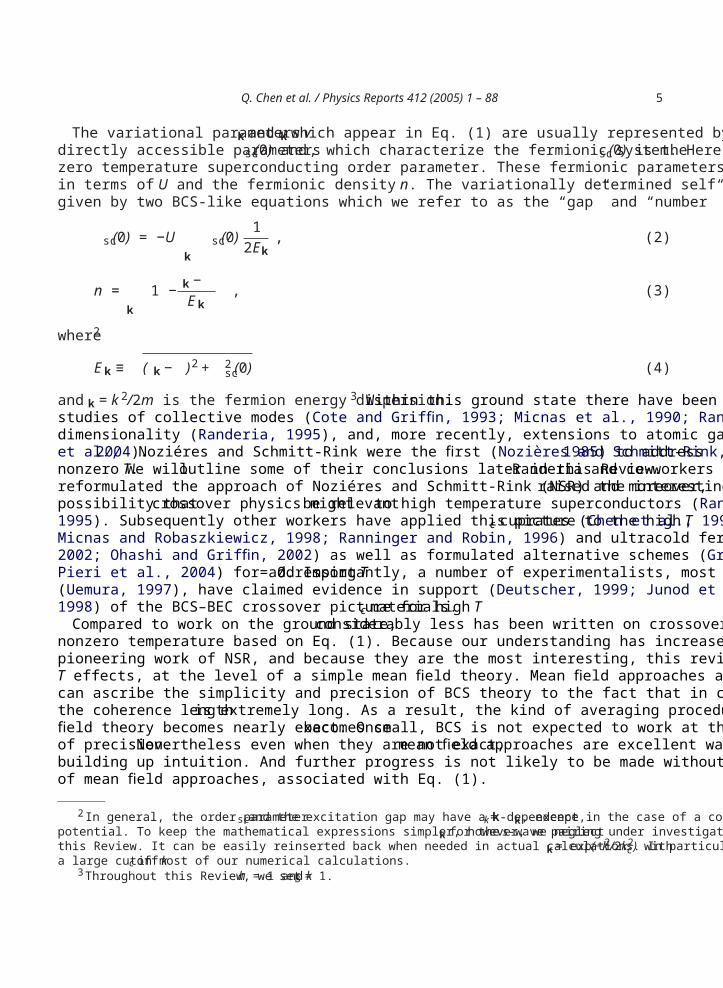
Fig. 2. Typical behavior of the T = 0 chemical potential in the three regimes. As the pairing strength increases from 0, thechemical potential starts to decrease and then becomes negative. The character of the system changes from fermionic ( >0)to bosonic ( <0). The PG (pseudogap) case corresponds to nonFermi liquid based superconductivity, and Uc corresponds tocritical coupling for forming a two fermion bound state in vacuum, as in Eq. (17) below.
The effects of BEC–BCS crossover are most directly reflected in the behavior of the fermionic chemicalpotential . We plot the behavior of in Fig. 2, which indicates the BCS and BEC regimes. In the weakcoupling regime = EF and ordinary BCS theory results. However at sufficiently strong coupling,begins to decrease, eventually crossing zero and then ultimately becoming negative in the BEC regime,with increasing |U |. We generally view =0 as a crossing point. For positive the system has a remnantFermi surface, and we say that it is “fermionic”. For negative , the Fermi surface is gone and the materialis “bosonic”.
The new and largely unexplored physics of this problem lies in the fact that once outside the BCS regime,but before BEC, superconductivity or superfluidity emerge out of a very exotic, non-Fermi liquid normalstate. Indeed, it should be clear that Fermi liquid theory must break down somewhere in the intermediateregime, as one goes continuously from fermionic to bosonic statistics. This intermediate case has manynames: “resonant superfluidity”, the “unitary regime” or, as we prefer (because it is more descriptive ofthe many body physics) the “pseudogap (PG) regime”. The PG regime plotted in Fig. 2 is drawn so thatits boundary on the left coincides with the onset of an appreciable excitation gap at Tc, called (Tc); itsboundary on the right coincides with where = 0. This non-Fermi liquid based superconductivity hasbeen extensively studied (Chen et al., 1998, 2000; Jankó et al., 1997; Maly et al., 1999a).
Fermi liquid theory is inappropriate here principally because there is a gap for creating fermionicexcitations. The non-Fermi liquid like behavior is reflected in that of the fermionic spectral function(Maly et al., 1999a) which has a two-peak structure in the normal state, broadened somewhat, but rathersimilar to its counterpart in BCS theory. Importantly, the onset of superconductivity occurs in the pres-ence of fermion pairs, which reflect this excitation gap. Unlike their counterparts in the BEC limit,these pairs are not infinitely long lived. Their presence is apparent even in the normal state where anenergy must be applied to create fermionic excitations. This energy cost derives from the breaking of themetastable pairs. Thus we say that there is a “pseudogap” at and aboveTc. But pseudogap effects are notrestricted to this normal state. Pre-formed pairs have a natural counterpart in the superfluid phase, as non-condensed pairs.
Q. Chen et al. / Physics Reports 412 (2005) 1 – 88 7
∆
∆(Τ)
Τc T*
∆sc
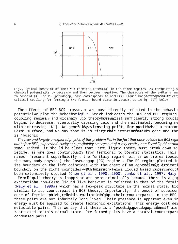
Fig. 3. Contrasting behavior of the excitation gap (T )and superfluid order parameter sc(T )versus temperature. The heightof the shaded region roughly reflects the density of noncondensed pairs at each temperature.
It will be stressed throughout this Review that gaps in the fermionic spectrum and bosonic degrees offreedom are two sides of the same coin. A particularly important observation to make is that the startingpoint for crossover physics is based on the fermionic degrees of freedom. Bosonic degrees of freedomare deduced from these; they are not primary. A nonzero value of the excitation gap is equivalent to thepresence of metastable or stable fermion pairs. And it is only in this indirect fashion that we can probethe presence of these “bosons”, within the framework of Eq. (1).
In many ways this crossover theory appears to represent a more generic form of superfluidity. Withoutdoing any calculations we can anticipate some of the effects of finite temperature. Except for very weakcoupling, pairs form and condense at different temperatures. The BCS limit might be viewed as theanomaly. Because the attractive interaction is presumed to be arbitrarily weak, in BCS the normal stateis unaffected by U and superfluidity appears precipitously, that is without warning atTc. More generally,in the presence of a moderately strong attractive interaction it pays energetically to take some advantageand to form pairs (say roughly at temperature T∗) within the normal state. Then, for statistical reasonsthese bosonic degrees of freedom ultimately are driven to condense at Tc < T∗, just as in BEC.
Just as there is a distinction betweenTc and T∗, there must be a distinction between the superconductingorder parameter sc and the excitation gap . The presence of a normal state excitation gap or pseudogapfor fermions is inextricably connected to this generalized BCS wavefunction. In Fig. 3, we present aschematic plot of these two energy parameters. It may be seen that the order parameter vanishes atTc, asin a second order phase transition, while the excitation gap turns on smoothly below T∗. It should alsobe stressed that there is only one gap energy scale in the ground state (Leggett, 1980) of Eq. (1). Thus atzero temperature
sc(0) = (0) . (5)
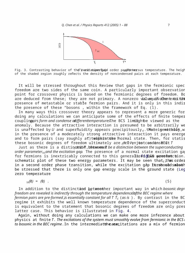
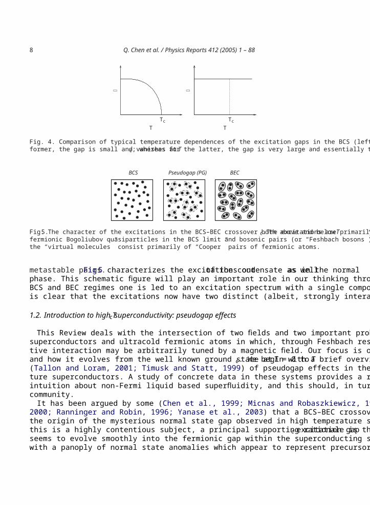
In addition to the distinction between and sc, another important way in which bosonic degrees offreedom are revealed is indirectly through the temperature dependence of . In the BEC regime wherefermion pairs are pre-formed, is essentially constant for all T ⩽Tc (as is ). By contrast in the BCSregime it exhibits the well known temperature dependence of the superconducting order parameter. Thisis equivalent to the statement that bosonic degrees of freedom are only present in the condensate for thislatter case. This behavior is illustrated in Fig. 4.
Again, without doing any calculations we can make one more inference about the nature of crossoverphysics at finite T. The excitations of the system must smoothly evolve from fermionic in the BCS regimeto bosonic in the BEC regime. In the intermediate case, the excitations are a mix of fermions and
8 Q. Chen et al. / Physics Reports 412 (2005) 1 – 88
Tc
T TTc
∆∆
Fig. 4. Comparison of typical temperature dependences of the excitation gaps in the BCS (left) and BEC (right) limits. For theformer, the gap is small and vanishes atTc; whereas for the latter, the gap is very large and essentially temperature independent.
BCS Pseudogap (PG) BEC
Fig. 5. The character of the excitations in the BCS–BEC crossover both above and below Tc. The excitations are primarilyfermionic Bogoliubov quasiparticles in the BCS limit and bosonic pairs (or “Feshbach bosons”) in the BEC limit. In the PG casethe “virtual molecules” consist primarily of “Cooper” pairs of fermionic atoms.
metastable pairs. Fig. 5 characterizes the excitations out of the condensate as well as in the normalphase. This schematic figure will play an important role in our thinking throughout this review. In theBCS and BEC regimes one is led to an excitation spectrum with a single component. For the PG case itis clear that the excitations now have two distinct (albeit, strongly interacting) components.
1.2. Introduction to high Tc superconductivity: pseudogap effects
This Review deals with the intersection of two fields and two important problems: high temperaturesuperconductors and ultracold fermionic atoms in which, through Feshbach resonance effects, the attrac-tive interaction may be arbitrarily tuned by a magnetic field. Our focus is on the broken symmetry phaseand how it evolves from the well known ground state at T = 0 to Tc. We begin with a brief overview(Tallon and Loram, 2001; Timusk and Statt, 1999) of pseudogap effects in the hole doped high tempera-ture superconductors. A study of concrete data in these systems provides a rather natural way of buildingintuition about non-Fermi liquid based superfluidity, and this should, in turn, be useful for the cold atomcommunity.
It has been argued by some (Chen et al., 1999; Micnas and Robaszkiewicz, 1998; Pieri and Strinati,2000; Ranninger and Robin, 1996; Yanase et al., 2003) that a BCS–BEC crossover-induced pseudogap isthe origin of the mysterious normal state gap observed in high temperature superconductors. Although,this is a highly contentious subject, a principal supporting rationale is that this above- Tc excitation gapseems to evolve smoothly into the fermionic gap within the superconducting state. This, in conjunctionwith a panoply of normal state anomalies which appear to represent precursor superconductivity effects,
Q. Chen et al. / Physics Reports 412 (2005) 1 – 88 9
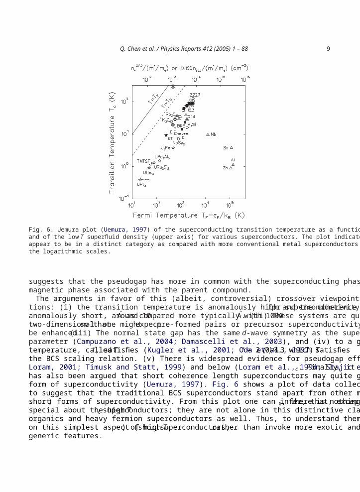
Fig. 6. Uemura plot (Uemura, 1997) of the superconducting transition temperature as a function of Fermi temperature (lower axis)and of the low T superfluid density (upper axis) for various superconductors. The plot indicates how “exotic” superconductorsappear to be in a distinct category as compared with more conventional metal superconductors such as Nb, Sn, Al and Zn. Notethe logarithmic scales.
suggests that the pseudogap has more in common with the superconducting phase than with the insulatingmagnetic phase associated with the parent compound.
The arguments in favor of this (albeit, controversial) crossover viewpoint rest on the following observa-tions: (i) the transition temperature is anomalously high and the coherence length for superconductivityanomalously short, around 10 A as compared more typically with 1000 A. (ii) These systems are quasi-two-dimensional so that one might expect pre-formed pairs or precursor superconductivity effects tobe enhanced. (iii) The normal state gap has the same d-wave symmetry as the superconducting orderparameter (Campuzano et al., 2004; Damascelli et al., 2003), and (iv) to a good approximation its onsettemperature, called T∗, satisfies (Kugler et al., 2001; Oda et al., 1997) T∗≈ 2 (0)/4.3 which satisfiesthe BCS scaling relation. (v) There is widespread evidence for pseudogap effects both above (Tallon andLoram, 2001; Timusk and Statt, 1999) and below (Loram et al., 1994; Stajic et al., 2003b) Tc. Finally, ithas also been argued that short coherence length superconductors may quite generally exhibit a distinctiveform of superconductivity (Uemura, 1997). Fig. 6 shows a plot of data collected by Uemura which seemsto suggest that the traditional BCS superconductors stand apart from other more exotic (and frequentlyshort ) forms of superconductivity. From this plot one can infer, that, except for highTc, there is nothingspecial about the high Tc superconductors; they are not alone in this distinctive class which includes theorganics and heavy fermion superconductors as well. Thus, to understand them, one might want to focuson this simplest aspect (short ) of high Tc superconductors, rather than invoke more exotic and lessgeneric features.
10 Q. Chen et al. / Physics Reports 412 (2005) 1 – 88
Hole concentration x
Tem
pera
ture
T
AFM
Pseudo Gap
Tc
T*
SC
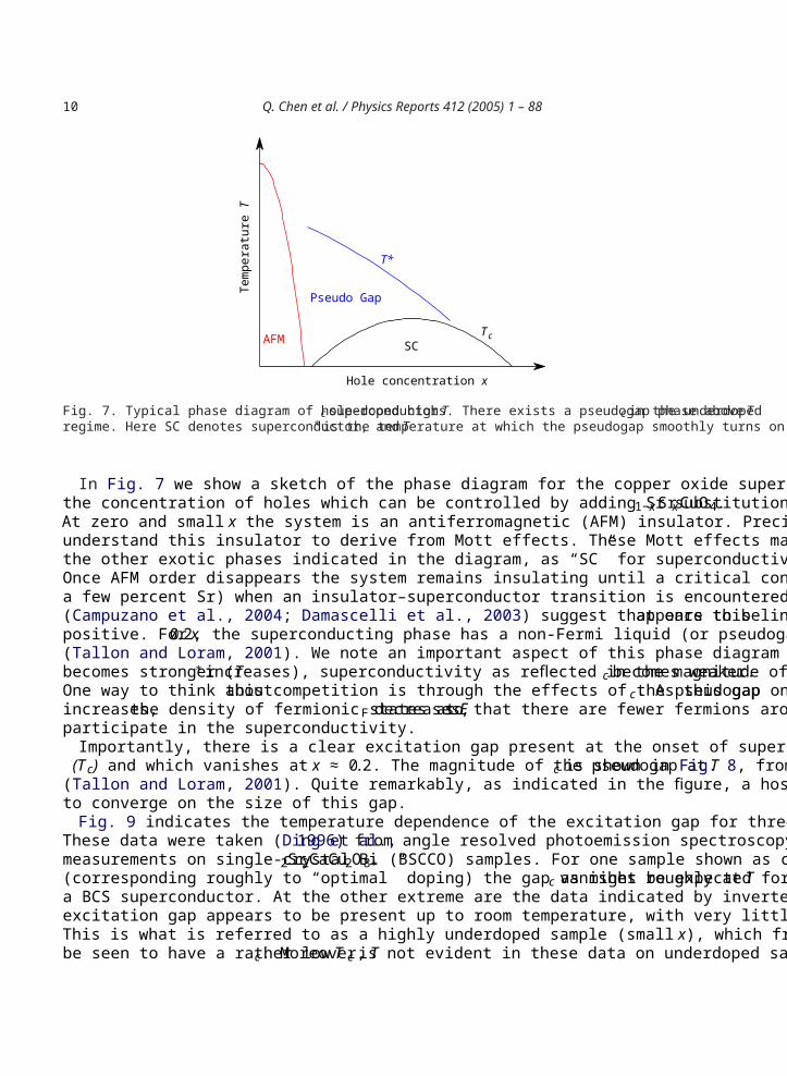
Fig. 7. Typical phase diagram of hole-doped highTc superconductors. There exists a pseudogap phase aboveTc in the underdopedregime. Here SC denotes superconductor, andT∗is the temperature at which the pseudogap smoothly turns on.
In Fig. 7 we show a sketch of the phase diagram for the copper oxide superconductors. Here x representsthe concentration of holes which can be controlled by adding Sr substitutionally, say, to La1−xSrxCuO4.At zero and small x the system is an antiferromagnetic (AFM) insulator. Precisely at half filling (x =0) weunderstand this insulator to derive from Mott effects. These Mott effects may or may not be the source ofthe other exotic phases indicated in the diagram, as “SC” for superconductivity and the pseudogap phase.Once AFM order disappears the system remains insulating until a critical concentration (typically arounda few percent Sr) when an insulator–superconductor transition is encountered. Here photoemission studies(Campuzano et al., 2004; Damascelli et al., 2003) suggest that once this line is crossed, appears to bepositive. For x⩽0.2, the superconducting phase has a non-Fermi liquid (or pseudogapped) normal state(Tallon and Loram, 2001). We note an important aspect of this phase diagram at low x. As the pseudogapbecomes stronger (T∗increases), superconductivity as reflected in the magnitude ofTc becomes weaker.One way to think about this competition is through the effects of the pseudogap on Tc. As this gapincreases, the density of fermionic states at EF decreases, so that there are fewer fermions around toparticipate in the superconductivity.
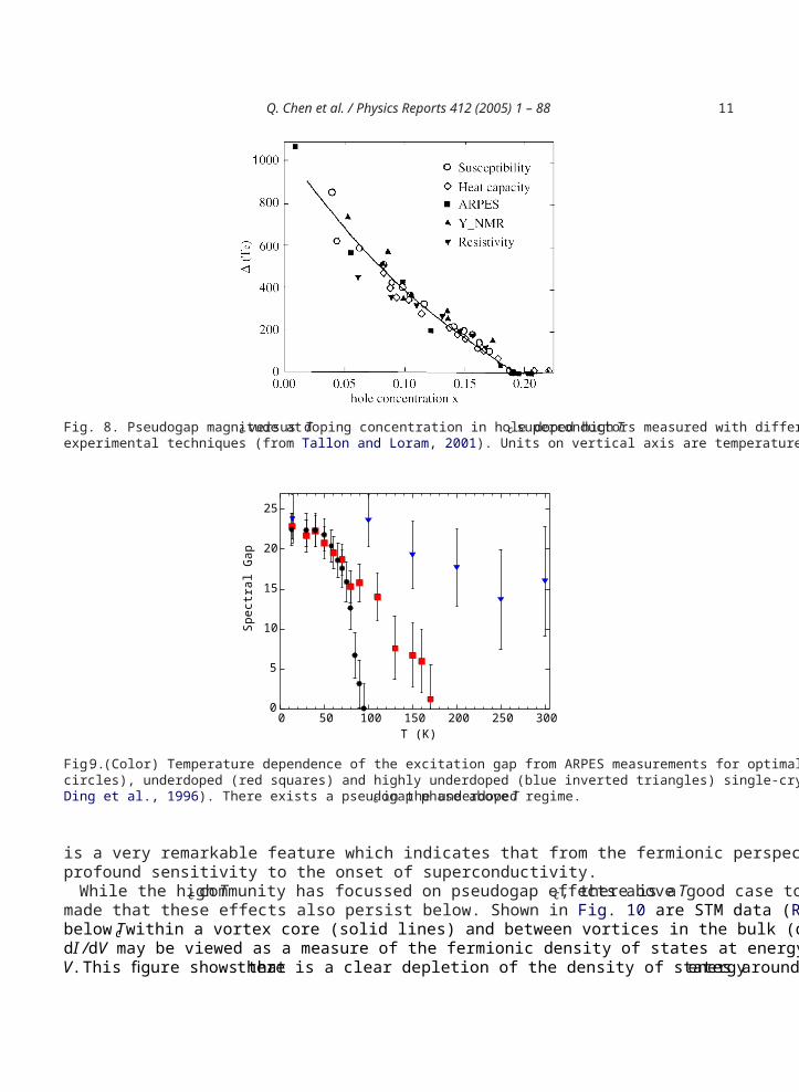
Importantly, there is a clear excitation gap present at the onset of superconductivity which is called(Tc) and which vanishes at x ≈ 0.2. The magnitude of the pseudogap at Tc is shown in Fig. 8, from
(Tallon and Loram, 2001). Quite remarkably, as indicated in the figure, a host of different probes seemto converge on the size of this gap.
Fig. 9 indicates the temperature dependence of the excitation gap for three different hole stoichiometries.These data were taken (Ding et al., 1996) from angle resolved photoemission spectroscopy (ARPES)measurements on single-crystal Bi2Sr2CaCu2O8+ (BSCCO) samples. For one sample shown as circles,(corresponding roughly to “optimal” doping) the gap vanishes roughly at Tc as might be expected fora BCS superconductor. At the other extreme are the data indicated by inverted triangles in which anexcitation gap appears to be present up to room temperature, with very little temperature dependence.This is what is referred to as a highly underdoped sample (small x), which from the phase diagram canbe seen to have a rather low Tc. Moreover, Tc is not evident in these data on underdoped samples. This
Q. Chen et al. / Physics Reports 412 (2005) 1 – 88 11
Fig. 8. Pseudogap magnitude atTc versus doping concentration in hole doped highTc superconductors measured with differentexperimental techniques (from Tallon and Loram, 2001). Units on vertical axis are temperature in degrees K.
0
5
10
15
20
25
0 50 100 150 200 250 300T (K)
Spec
tral G
ap
Fig. 9. (Color) Temperature dependence of the excitation gap from ARPES measurements for optimally doped (filled blackcircles), underdoped (red squares) and highly underdoped (blue inverted triangles) single-crystal BSCCO samples (taken fromDing et al., 1996). There exists a pseudogap phase aboveTc in the underdoped regime.
is a very remarkable feature which indicates that from the fermionic perspective there appears to be noprofound sensitivity to the onset of superconductivity.
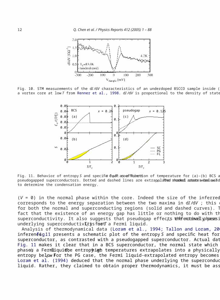
While the high Tc community has focussed on pseudogap effects above Tc, there is a good case to bemade that these effects also persist below. Shown in Fig. 10 are STM data (Renner et al., 1998) takenbelow Tc within a vortex core (solid lines) and between vortices in the bulk (dashed lines). The quantitydI /dV may be viewed as a measure of the fermionic density of states at energy E given by the voltageV. This figure shows that there is a clear depletion of the density of states around the Fermi energy
12 Q. Chen et al. / Physics Reports 412 (2005) 1 – 88
Fig. 10. STM measurements of the dI /dV characteristics of an underdoped BSCCO sample inside (solid) and outside (dashed)a vortex core at low T from Renner et al., 1998. dI /dV is proportional to the density of states.
0
0.01
0.02
0.03
0.04
0.05
Cv
/(T/T
c)
10 2T/Tc
0
0.02
0.04
S
0
0.1
0.2
T/Tc
0
0.1
0.2
SCPGFL
BCS pseudogapx = 0.25 x = 0.125
(a)
(b) (d)
(c)
0 1 2 3
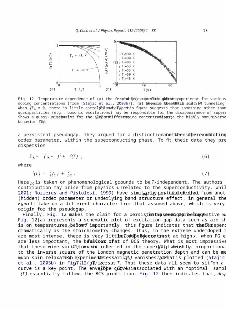
Fig. 11. Behavior of entropy S and specific heat coefficient ≡ Cv/T as a function of temperature for (a)–(b) BCS and (c)–(d)pseudogapped superconductors. Dotted and dashed lines are extrapolated normal states belowTc. The shaded areas were usedto determine the condensation energy.
(V = 0) in the normal phase within the core. Indeed the size of the inferred energy gap (or pseudogap)corresponds to the energy separation between the two maxima in dI /dV ; this can be seen to be the samefor both the normal and superconducting regions (solid and dashed curves). This figure emphasizes thefact that the existence of an energy gap has little or nothing to do with the existence of phase coherentsuperconductivity. It also suggests that pseudogap effects effectively persist below Tc; the normal phaseunderlying superconductivity for T ⩽Tc is not a Fermi liquid.
Analysis of thermodynamical data (Loram et al., 1994; Tallon and Loram, 2001) has led to a similarinference. Fig. 11 presents a schematic plot of the entropy S and specific heat for the case of a BCSsuperconductor, as contrasted with a pseudogapped superconductor. Actual data are presented in Fig. 38.Fig. 11 makes it clear that in a BCS superconductor, the normal state which underlies the superconductingphase, is a Fermi liquid; the entropy at high temperatures extrapolates into a physically meaningfulentropy below Tc. For the PG case, the Fermi liquid-extrapolated entropy becomes negative. In this wayLoram et al. (1994) deduced that the normal phase underlying the superconducting state is not a Fermiliquid. Rather, they claimed to obtain proper thermodynamics, it must be assumed that this state contains
Q. Chen et al. / Physics Reports 412 (2005) 1 – 88 13
0 40 80T(K)
-30
-15
0
ρ s(T
)-ρ s
(0)(
meV
)
Tc=90 KTc=90 KTc=88 KTc=65 KTc=55 KTc=50 KTc=48 K
0T / Tc
0
1 ∆
(T) /
∆(0)
Tc = 48 K
Tc = 90 K
1(a) (b)
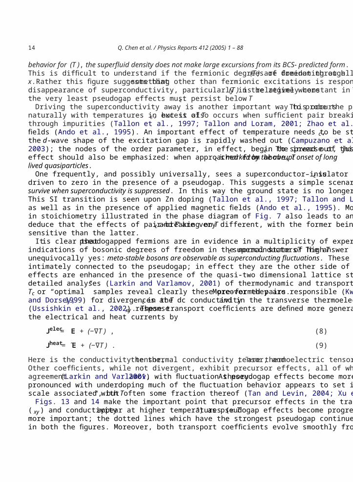
Fig. 12. Temperature dependence of (a) the fermionic excitation gap and (b) superfluid density s from experiment for variousdoping concentrations (from (Stajic et al., 2003b)). (a) Shows a schematic plot ofas seen in the ARPES and STM tunneling data.When (Tc) = 0, there is little correlation between (T )and s(T ); this figure suggests that something other than fermionicquasiparticles (e.g., bosonic excitations) may be responsible for the disappearance of superconductivity with increasing T. (b)Shows a quasi-universal behavior for the slope d s/dT at different doping concentrations, despite the highly nonuniversalbehavior for (T ).
a persistent pseudogap. They argued for a distinction between the excitation gapand the superconductingorder parameter, within the superconducting phase. To fit their data they presumed a modified fermionicdispersion
Ek = ( k − )2 + 2(T ) , (6)
where2(T ) = 2
sc(T ) + 2pg . (7)
Here pg is taken on phenomenological grounds to be T-independent. The authors argue that the pseudogapcontribution may arise from physics unrelated to the superconductivity. While others (Chakravarty et al.,2001; Nozieres and Pistolesi, 1999) have similarly postulated that pg may in fact derive from another(hidden) order parameter or underlying band structure effect, in general the fermionic dispersion relationEk will take on a different character from that assumed above, which is very specific to a superconductingorigin for the pseudogap.
Finally, Fig. 12 makes the claim for a persistent pseudogap belowTc in an even more suggestive way.Fig. 12(a) represents a schematic plot of excitation gap data such as are shown in Fig. 9. Here the focusis on temperatures below Tc. Most importantly, this figure indicates that the T dependence in variesdramatically as the stoichiometry changes. Thus, in the extreme underdoped regime, where PG effectsare most intense, there is very little T dependence in below Tc. By contrast at high x, when PG effectsare less important, the behavior of follows that of BCS theory. What is most impressive however, isthat these wide variations in (T )are not reflected in the superfluid density s(T ), which is proportionalto the inverse square of the London magnetic penetration depth and can be measured by, for example,muon spin relaxation ( SR) experiments. Necessarily, s(T ) vanishes at Tc. What is plotted (Stajicet al., 2003b) in Fig. 12(b) is s(T ) − s(0) versus T. That these data all seem to sit on a rather universalcurve is a key point. The envelope curve in s(T ) − s(0) is associated with an “optimal” sample where(T )essentially follows the BCS prediction. Fig. 12 then indicates that, despite the highly nonuniversal
14 Q. Chen et al. / Physics Reports 412 (2005) 1 – 88
behavior for (T ), the superfluid density does not make large excursions from its BCS- predicted form.This is difficult to understand if the fermionic degrees of freedom through (T )are dominating at allx. Rather this figure suggests that something other than fermionic excitations is responsible for thedisappearance of superconductivity, particularly in the regime where (T )is relatively constant in T. Atthe very least pseudogap effects must persist below Tc.
Driving the superconductivity away is another important way to probe the pseudogap. This occursnaturally with temperatures in excess of Tc, but it also occurs when sufficient pair breaking is presentthrough impurities (Tallon et al., 1997; Tallon and Loram, 2001; Zhao et al., 1993) or applied magneticfields (Ando et al., 1995). An important effect of temperature needs to be stressed. With increasingT > Tc,the d-wave shape of the excitation gap is rapidly washed out (Campuzano et al., 2004; Damascelli et al.,2003); the nodes of the order parameter, in effect, begin to spread out, just above Tc. The inverse of thiseffect should also be emphasized: when approached from above,Tc is marked by the abrupt onset of longlived quasiparticles.
One frequently, and possibly universally, sees a superconductor–insulator (SI) transition when Tc isdriven to zero in the presence of a pseudogap. This suggests a simple scenario: that the pseudogap maysurvive when superconductivity is suppressed. In this way the ground state is no longer a simple metal.This SI transition is seen upon Zn doping (Tallon et al., 1997; Tallon and Loram, 2001; Zhao et al., 1993),as well as in the presence of applied magnetic fields (Ando et al., 1995). Moreover, the intrinsic changein stoichiometry illustrated in the phase diagram of Fig. 7 also leads to an SI transition. One can thusdeduce that the effects of pair-breaking on Tc and T∗are very different, with the former being far moresensitive than the latter.
It is clear that pseudogapped fermions are in evidence in a multiplicity of experiments. Are thereindications of bosonic degrees of freedom in the normal state of highTc superconductors? The answer isunequivocally yes: meta-stable bosons are observable as superconducting fluctuations. These bosons areintimately connected to the pseudogap; in effect they are the other side of the same coin. These bosoniceffects are enhanced in the presence of the quasi-two dimensional lattice structure of these materials. Verydetailed analyses (Larkin and Varlamov, 2001) of thermodynamic and transport properties of the highestTc or “optimal” samples reveal clearly these pre-formed pairs. Moreover they are responsible (Kwonand Dorsey, 1999) for divergences at Tc in the dc conductivity and in the transverse thermoelectric(Ussishkin et al., 2002) response xy. These transport coefficients are defined more generally in terms ofthe electrical and heat currents by
Jelec = E + (−∇T ) , (8)
Jheat = E + (−∇T ) . (9)
Here is the conductivity tensor, the thermal conductivity tensor, and , ˜are thermoelectric tensors.Other coefficients, while not divergent, exhibit precursor effects, all of which are found to be in goodagreement (Larkin and Varlamov, 2001) with fluctuation theory. As pseudogap effects become morepronounced with underdoping much of the fluctuation behavior appears to set in at a higher temperaturescale associated with T∗, but often some fraction thereof (Tan and Levin, 2004; Xu et al., 2000).
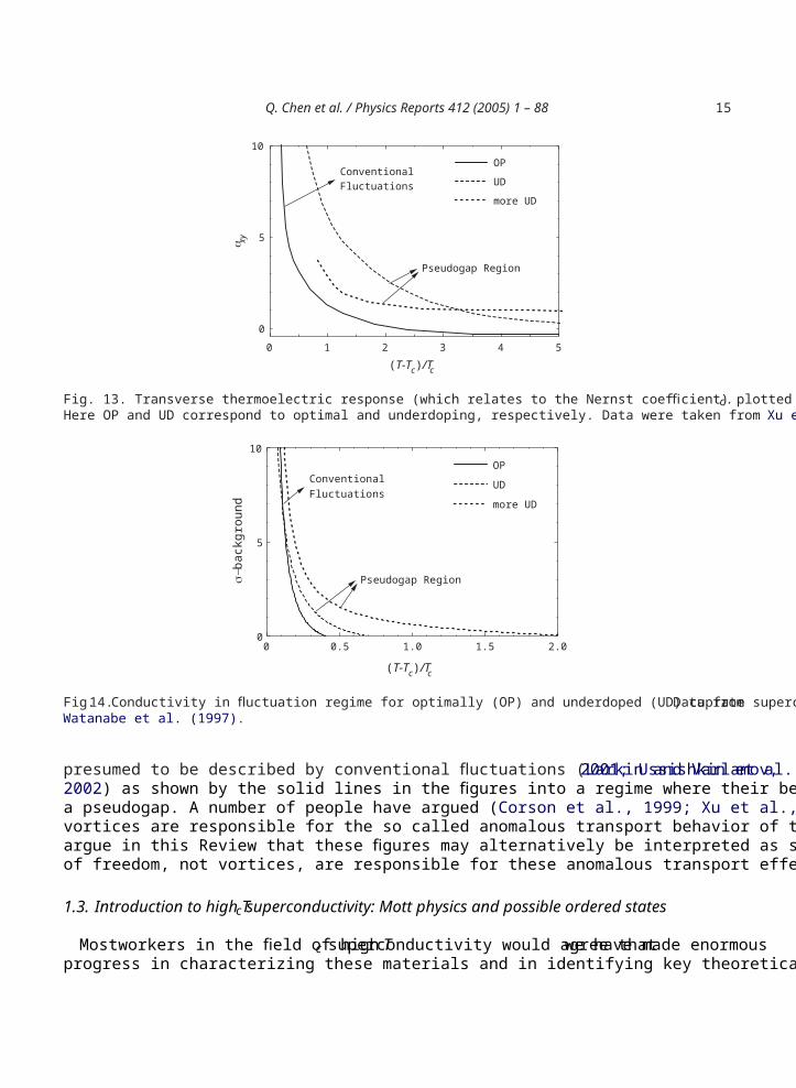
Figs. 13 and 14 make the important point that precursor effects in the transverse thermoelectric response( xy) and conductivity appear at higher temperatures (∝ T∗) as pseudogap effects become progressivelymore important; the dotted lines which have the strongest pseudogap continue to the highest temperaturesin both the figures. Moreover, both transport coefficients evolve smoothly from a regime where they are
Q. Chen et al. / Physics Reports 412 (2005) 1 – 88 15
(T-Tc)/Tc
0 1 2 3 4 5
0
5
10
more UD
UD
OPConventionalFluctuations
Pseudogap Region
αxy
Fig. 13. Transverse thermoelectric response (which relates to the Nernst coefficient) plotted here in fluctuation regime aboveTc.Here OP and UD correspond to optimal and underdoping, respectively. Data were taken from Xu et al. (2000).
(T-Tc)/Tc
σ−ba
ckgr
ound
0 0.5 1.0 1.5 2.00
5
10
more UD
UD
OPConventionalFluctuations
Pseudogap Region
Fig. 14. Conductivity in fluctuation regime for optimally (OP) and underdoped (UD) cuprate superconductors. Data fromWatanabe et al. (1997).
presumed to be described by conventional fluctuations (Larkin and Varlamov, 2001; Ussishkin et al.,2002) as shown by the solid lines in the figures into a regime where their behavior is associated witha pseudogap. A number of people have argued (Corson et al., 1999; Xu et al., 2000) that normal statevortices are responsible for the so called anomalous transport behavior of the pseudogap regime. We willargue in this Review that these figures may alternatively be interpreted as suggesting that bosonic degreesof freedom, not vortices, are responsible for these anomalous transport effects.
1.3. Introduction to high Tc superconductivity: Mott physics and possible ordered states
Most workers in the field of high Tc superconductivity would agree that we have made enormousprogress in characterizing these materials and in identifying key theoretical questions and constructs.
16 Q. Chen et al. / Physics Reports 412 (2005) 1 – 88
Experimental progress, in large part, comes from transport studies (Tallon and Loram, 2001; Timuskand Statt, 1999) in addition to three powerful spectroscopies: photoemission (Campuzano et al., 2004;Damascelli et al., 2003), neutron (Aeppli et al., 1997a, b; Cheong et al., 1991; Fong et al., 1995; Kastneret al., 1998; Mook et al., 1998; Rossat-Mignod et al., 1991; Tranquada et al., 1992) and Josephsoninterferometry (Wollman et al., 1995; Tsuei et al., 1994; Mathai et al., 1995). These data have provided uswith important clues to address related theoretical challenges. Among the outstanding theoretical issuesin the cuprates are (i) understanding the attractive “mechanism” that binds electrons into Cooper pairs,(ii) understanding the evolution of the normal phase from Fermi liquid (in the “overdoped” regime) tomarginal Fermi liquid (at “optimal” doping) to the pseudogap state, which is presumed to occur as dopingconcentration x decreases, and (iii) understanding the nature of that superconducting phase which evolvesfrom each of these three normal states.
The theoretical community has concentrated rather extensively on special regions and x-dependences inthe phase diagram which are presumed to be controlled by “Mott physics”. There are different viewpointson precisely what constitutes Mott physics in the metallic phases, and, for example, whether or notthis is necessarily associated with spin-charge separation. For the most part, one presumes here that theinsulating phase of the parent compound introduces strong Coulomb correlations into the doped metallicstates which may or may not also be associated with strong antiferromagnetic correlations. There isa recent, rather complete review (Lee et al., 2004) of Mott physics within the scenario of spin-chargeseparation, which clarifies the physics it entails.
Concrete experimental signatures of Mott physics are the observations that the superfluid densitys(T = 0, x) → 0 as x → 0, as if it were reflecting an order parameter for a metal insulator transition.
More precisely it is deduced that s(0, x) ∝ x, at low x. Unusual effects associated with this linear- in- xdependence also show up in other experiments, such as the weight of coherence features in photoemissiondata (Campuzano et al., 2004; Damascelli et al., 2003), as well as in thermodynamical signatures (Tallonand Loram, 2001).
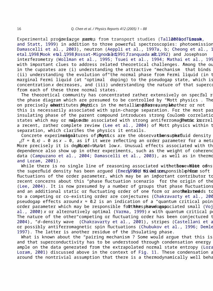
While there is no single line of reasoning associated with these Mott constraints, the low value ofthe superfluid density has been argued (Emery and Kivelson, 1995) to be responsible for soft phasefluctuations of the order parameter, which may be an important contributor to the pseudogap. However,recent concerns about this “phase fluctuation scenario” for the origin of the pseudogap have been raised(Lee, 2004). It is now presumed by a number of groups that phase fluctuations alone may not be adequateand an additional static or fluctuating order of one form or another needs to be incorporated. Relatedto a competing or co-existing order are conjectures (Chakravarty et al., 2001) that the disappearance ofpseudogap effects around x ≈ 0.2 is an indication of a “quantum critical point” associated with a hiddenorder parameter which may be responsible for the pseudogap. Others have associated small (Vojta etal., 2000) x or alternatively optimal (Varma, 1999) x with quantum critical points of a different origin.The nature of the other competing or fluctuating order has been conjectured to be RVB (Anderson et al.,2004), “d-density wave” (Chakravarty et al., 2001), stripes (Castellani et al., 1995; Zachar et al., 1997)or possibly antiferromagnetic spin fluctuations (Chubukov et al., 1996; Demler and Zhang, 1995; Pines,1997). The latter is another residue of the insulating phase.
What is known about the “pairing mechanism”? Some would argue that this is an ill-defined question,and that superconductivity has to be understood through condensation energy arguments based for ex-ample on the data generated from the extrapolated normal state entropy (Loram et al., 1994; Tallon andLoram, 2001) discussed above in the context of Fig. 11. These condensation arguments are often builtaround the nontrivial assumption that there is a thermodynamically well behaved but meta-stable normal
Q. Chen et al. / Physics Reports 412 (2005) 1 – 88 17
phase which coexists with the superconductivity. Others would argue that Coulomb effects are responsiblefor d-wave pairing, either directly (Leggett, 1999; Liu and Levin, 1997), or indirectly via magnetic fluc-tuations (Pines, 1997; Scalapino et al., 1986). Moreover, the extent to which the magnetism is presumedto persist into the metallic phase near optimal doping is controversial. Initially, NMR measurements wereinterpreted as suggesting (Millis et al., 1990) strong antiferromagnetic fluctuations, while neutron mea-surements, which are generally viewed as the more conclusive, do not provide compelling evidence (Siet al., 1993) for their presence in the normal phase. Nevertheless, there are interesting neutron-measuredmagnetic signatures (Kao et al., 2000; Liu et al., 1995; Zha et al., 1993) belowTc associated with d-wavesuperconductivity. There are also analogous STM effects which are currently of interest (Wang and Lee,2003).
1.4. Overview of the BCS–BEC picture of high Tc superconductors in the underdoped regime
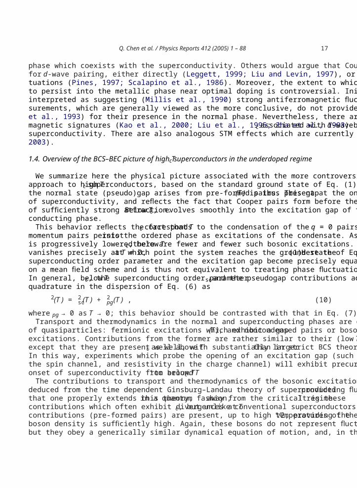
We summarize here the physical picture associated with the more controversial BCS–BEC crossoverapproach to high Tc superconductors, based on the standard ground state of Eq. (1). One presumes thatthe normal state (pseudo)gap arises from pre-formed pairs. This gap (T ) is thus present at the onsetof superconductivity, and reflects the fact that Cooper pairs form before they Bose condense, as a resultof sufficiently strong attraction. Below Tc, evolves smoothly into the excitation gap of the super-conducting phase.
This behavior reflects the fact that Tc corresponds to the condensation of the q =0 pairs, while finitemomentum pairs persist into the ordered phase as excitations of the condensate. As the temperatureis progressively lowered below Tc, there are fewer and fewer such bosonic excitations. Their numbervanishes precisely at T = 0, at which point the system reaches the ground state of Eq. (1). Here thesuperconducting order parameter and the excitation gap become precisely equal. This approach is basedon a mean field scheme and is thus not equivalent to treating phase fluctuations of the order parameter.In general, below Tc, the superconducting order parameter sc and the pseudogap contributions add inquadrature in the dispersion of Eq. (6) as
2(T ) = 2sc(T ) + 2
pg(T ) , (10)
where pg → 0 as T → 0; this behavior should be contrasted with that in Eq. (7).Transport and thermodynamics in the normal and superconducting phases are determined by two types
of quasiparticles: fermionic excitations which exhibit a gap (T ), and noncondensed pairs or bosonicexcitations. Contributions from the former are rather similar to their (low T) counterparts in BCS theory,except that they are present well above Tc as well, with substantially larger than in strict BCS theory.In this way, experiments which probe the opening of an excitation gap (such as Pauli susceptibility inthe spin channel, and resistivity in the charge channel) will exhibit precursor effects, that is, the gradualonset of superconductivity from around T∗to below Tc.
The contributions to transport and thermodynamics of the bosonic excitations are rather similar to thosededuced from the time dependent Ginsburg–Landau theory of superconducting fluctuations, providedthat one properly extends this theory, in a quantum fashion, away from the critical regime. It is thesecontributions which often exhibit divergences at Tc, but unlike conventional superconductors, bosoniccontributions (pre-formed pairs) are present, up to high temperatures of the order ofT∗/2, providing theboson density is sufficiently high. Again, these bosons do not represent fluctuations of the order parameter,but they obey a generically similar dynamical equation of motion, and, in the more general case which
18 Q. Chen et al. / Physics Reports 412 (2005) 1 – 88
goes beyond Eq. (1), they will be coupled to order parameter fluctuations. Here, in an oversimplifiedsense there is a form of spin-charge separation. The bosons are spin-less (singlet) with charge 2 e, whilethe fermions carry both spin and charge, but are non-Fermi-liquid like, as a consequence of their energygap.
In the years following the discovery of high Tc superconductors, attention focused on the so-calledmarginal Fermi liquid behavior of the cuprates. This phase is associated with near-optimal doping. Themost salient signature of this marginality is the dramatically linear in temperature dependence of theresistivity from just above Tc to very high temperatures, well above room temperature. Today, we knowthat pseudogap effects are present at optimal doping, so that the precise boundary between the marginaland pseudogap phases is not clear. As a consequence, addressing this normal state resistivity in theBCS–BEC crossover approach has not been done in detail, although it is unlikely to yield a strictly linearT dependence at a particular doping. Nevertheless, the bosonic contributions lead to a decrease in resistivityas temperature is lowered, while the opening of a d-wave gap associated with the fermionic terms leadsto an increase, which tends to compensate. These are somewhat analogous to Aslamazov–Larkin andMaki–Thompson fluctuation contributions (Larkin and Varlamov, 2001). The bosons generally dominatein the vicinity ofTc, but at higher T, in the vicinity ofT∗, the gapped fermions will be the more important.
The vanishing of Tc with sufficiently large T∗(extreme underdoping) occurs in an interesting way inthis crossover theory. This effect is associated with the localization of the bosonic degrees of freedom.Pauli principle effects in conjunction with the extended size of d-wave pairs inhibit pair hopping, andthus destroy superconductivity. One can speculate that, just as in conventional Bose systems, once thebosons are localized, they will exhibit an alternative form of long range order. Indeed, “pair density wave”models have been invoked (Chen et al., 2004) to explain recent STM data (Fu et al., 2004; Vershinin etal., 2004). In contrast to the cold atom systems, for the d-wave case the BEC regime is never accessed.This superconductor-insulator transition takes place in the fermionic regime where ≈ 0.8EF.
In the context of BCS–BEC crossover physics, it is not essential to establish the source of the attractiveinteraction. For the most part we skirt this issue in this Review by taking the pairing onset temperatureT∗(x) as a phenomenological input parameter. At the simplest level one may argue that as the systemapproaches the Mott insulating limit ( x → 0) fermions become less mobile; this serves to increase theeffectiveness of the attractive interaction at low doping levels.
The variable x in the high Tc problem should be viewed then, as a counterpart to the magnetic fieldvariable in the cold atom problem which tunes the system through a Feshbach resonance; both x andfield strength modulate the size of the attraction. However, for the cuprates, in contrast to the cold atomsystems, one never reaches the BEC limit of the crossover theory.
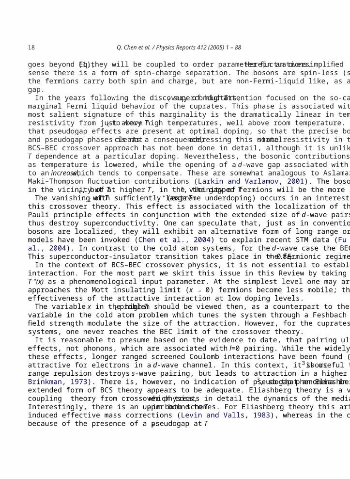
It is reasonable to presume based on the evidence to date, that pairing ultimately derives from Coulombiceffects, not phonons, which are associated withl=0 pairing. While the widely used Hubbard model ignoresthese effects, longer ranged screened Coulomb interactions have been found (Liu and Levin, 1997) to beattractive for electrons in a d-wave channel. In this context, it is useful to note that, similarly, in He3 shortrange repulsion destroys s-wave pairing, but leads to attraction in a higher (l =1) channel (Anderson andBrinkman, 1973). There is, however, no indication of pseudogap phenomena in He3, so that an Eliashbergextended form of BCS theory appears to be adequate. Eliashberg theory is a very different form of “strongcoupling” theory from crossover physics, which treats in detail the dynamics of the mediating boson.Interestingly, there is an upper bound to Tc in both schemes. For Eliashberg theory this arises from theinduced effective mass corrections (Levin and Valls, 1983), whereas in the crossover problem this occursbecause of the presence of a pseudogap at Tc.
Q. Chen et al. / Physics Reports 412 (2005) 1 – 88 19
Other analogies have also been invoked in comparing the cuprates with superfluid He 3, based on thepropensity towards magnetism. In the case of the quantum liquid, however, there is a positive correlationbetween short range magnetic ordering (Levin and Valls, 1983) and superconductivity while the correlationappears negative for the cuprates (and some of their heavy fermion “cousins”) where magnetism andsuperconductivity appear to compete.
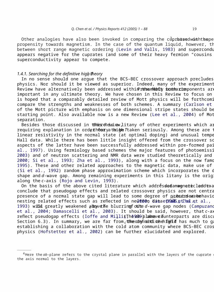
1.4.1. Searching for the definitive high Tc theoryIn no sense should one argue that the BCS–BEC crossover approach precludes consideration of Mott
physics. Nor should it be viewed as superior. Indeed, many of the experiments we will address in thisReview have alternatively been addressed within the Mott scenario. Presumably both components areimportant in any ultimate theory. We have chosen in this Review to focus on one component only, and itis hoped that a comparably detailed review of Mott physics will be forthcoming. In this way one couldcompare the strengths and weaknesses of both schemes. A summary (Carlson et al., 2002) of some aspectsof the Mott picture with emphasis on one dimensional stripe states should be referred to as a very usefulstarting point. Also available now is a new Review (Lee et al., 2004) of Mott physics, based on spin chargeseparation.
Besides those discussed in this Review, there is a litany of other experiments which are viewed asrequiring explanation in order for a high Tc theory to be taken seriously. Among these are the importantlinear resistivity in the normal state (at optimal doping) and unusual temperature and x dependences inHall data. While there has been little insight offered from the crossover scheme to explain the former,aspects of the latter have been successfully addressed within pre-formed pair scenarios (Geshkenbein etal., 1997). Using fermiology based schemes the major features of photoemission (Norman and Pepin,2003) and of neutron scattering and NMR data were studied theoretically and rather early on (Kao et al.,2000; Si et al., 1993; Zha et al., 1993), along with a focus on the now famous 41 meV feature (Liu et al.,1995). These and other related approaches to the magnetic data, make use of a microscopically derived(Si et al., 1992) random phase approximation scheme which incorporates the details of the Fermi surfaceshape and d-wave gap. Among remaining experiments in this litany is the origin of incoherent transportalong the c-axis (Rojo and Levin, 1993).
On the basis of the above cited literature which addressed magnetic and c-axis 4 data we are led toconclude that pseudogap effects and related crossover physics are not central to their understanding. Thepresence of a normal state gap will lead to some degree of precursor behavior above Tc, but d-wavenesting related effects such as reflected in neutron data (Kao et al., 2000; Liu et al., 1995; Zha et al.,1993) will be greatly weakened above Tc by the blurring out of the d-wave gap nodes (Campuzanoet al., 2004; Damascelli et al., 2003). It should be said, however, that c-axis optical data do appear toreflect pseudogap effects (Ioffe and Millis, 1999) above Tc. (The ab-plane counterparts are discussed inSection 6.3). In summary, we are far from the definitive highTc theory and the field has much to gain byestablishing a collaboration with the cold atom community where BCS–BEC crossover as well as Mottphysics (Hofstetter et al., 2002) can be further elucidated and explored.
4 Here the ab-plane refers to the crystal plane in parallel with the layers of the cuprate compounds, and the c-axis refers tothe axis normal to the layers.
20 Q. Chen et al. / Physics Reports 412 (2005) 1 – 88
Ener
gy
ν δ (B)
S=1
S=0
Internuclear distance
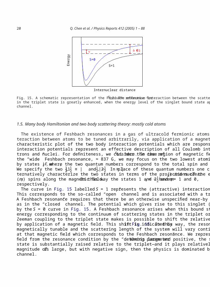
Fig. 15. A schematic representation of the Feshbach resonance for6Li. The effective interaction between the scattering of atomsin the triplet state is greatly enhanced, when the energy level of the singlet bound state approaches the continuum of theS =1channel.
1.5. Many body Hamiltonian and two body scattering theory: mostly cold atoms
The existence of Feshbach resonances in a gas of ultracold fermionic atoms allows the attractive in-teraction between atoms to be tuned arbitrarily, via application of a magnetic field. Fig. 15 presents acharacteristic plot of the two body interaction potentials which are responsible for this resonance. Theseinteraction potentials represent an effective description of all Coulomb interactions between the elec-trons and nuclei. For definiteness, we consider the case of 6Li here. In the region of magnetic fields nearthe “wide” Feshbach resonance, ≈ 837 G, we may focus on the two lowest atomic levels characterizedby states |F, mF , where the two quantum numbers correspond to the total spin and its z component.We specify the two |1 ≡ |1
2 , 12 and |2 ≡ |1
2 , −12 . In place of these quantum numbers one can al-
ternatively characterize the two states in terms of the projections of the electronic ( ms) and nuclear(mi ) spins along the magnetic field. In this way the states 1 and 2 have ms = −1
2 and mi = 1 and 0,respectively.
The curve in Fig. 15 labelled S =1 represents the (attractive) interaction between these two states.This corresponds to the so-called “open” channel and is associated with a triplet (electronic) spin state.A Feshbach resonance requires that there be an otherwise unspecified near-by state which we refer toas in the “closed” channel. The potential which gives rise to this singlet (electronic) spin state is shownby the S =0 curve in Fig. 15. A Feshbach resonance arises when this bound state lies near the zero ofenergy corresponding to the continuum of scattering states in the triplet or open channel. The electronicZeeman coupling to the triplet state makes is possible to shift the relative position of the two potentialsby application of a magnetic field. This shift is indicated by in Fig. 15. In this way, the resonance ismagnetically tunable and the scattering length of the system will vary continuously with field, divergingat that magnetic field which corresponds to the Feshbach resonance. We represent the deviation of thisfield from the resonance condition by the “detuning parameter” . When is large and positive, the singletstate is substantially raised relative to the triplet—and it plays relatively little role. By contrast when themagnitude of is large, but with negative sign, then the physics is dominated by the singlet or closedchannel.
Q. Chen et al. / Physics Reports 412 (2005) 1 – 88 21
The most general form for the Hamiltonian contains two types of particles: fermions which representthe open channel and “molecular bosons” which represent the two fermion bound state of the closedchannel. We will also refer to the latter as “Feshbach bosons”. These, in turn, lead to two types ofinteraction effects: those associated with the direct attraction between fermions, parameterized by U, andthose associated with “fermion–boson” interactions, whose strength is governed by g. The latter may beviewed as deriving from hyperfine interactions which couple the (total) nuclear and electronic spins. Inthe highTc applications, one generally, but not always, ignores the bosonic degrees of freedom. Otherwisethe Hamiltonians are the same, and can be written as
H − N =k,
( k − )a†k, ak, +
q( mb
q + − 2 )b†qbq
+q,k,k
U (k, k )a†q/2+k,↑a†
q/2−k,↓aq/2−k ,↓aq/2+k ,↑
+q,k
(g(k)b†qaq/2−k,↓aq/2+k,↑+ h.c.). (11)
Here the fermion and boson kinetic energies are given by k = k2/(2m), and mbq = q2/(2M) , and is
an important parameter which represents the magnetic field “detuning”. M = 2mis the bare mass of theFeshbach bosons. For the cold atom problem = ↑, ↓represents the two different hyperfine states ( |1and |2 ). One may ignore (Timmermans et al., 2001) the nondegeneracy of these two states, since there isno known way for state 2 to decay into state 1. In the two channel problem the ground state wavefunctionis slightly modified and given by
¯0 = 0 ⊗ B0 , (12)
where the normalized molecular boson contribution B0 is
B0 = e− 2/2+ b†
0 |0 . (13)
as discussed originally by Kostyrko and Ranninger, 1996. Here is a variational parameter. We presentthe resulting variational conditions for the ground state in Appendix A.
Whether both forms of interactions are needed in either the high Tc or cold atom systems is stillunder debate. The bosons (b†
k) of the cold atom problem (Holland et al., 2001; Timmermans et al., 2001)will be referred to as Feshbach bosons. These represent a separate species, not to be confused with thefermion pair (a†
ka†−k) operators. Thus we call this a “two channel” model. In this review we will discuss
the behavior of crossover physics both with and without these Feshbach bosons (FB). Previous studiesof high Tc superconductors have invoked a similar bosonic term (Geshkenbein et al., 1997; Micnas etal., 1990; Ranninger and Robin, 1996) as well, although less is known about its microscopic origin.This fermion–boson coupling is not to be confused with the coupling between fermions and a “pairing-mechanism”-related boson ([b+b†]a†a) such as phonons. The couplingb†aaand its conjugate representsa form of sink and source for creating fermion pairs, inducing superconductivity in some ways, as a by-product of Bose condensation. We will emphasize throughout that crossover theory proceeds in a similarfashion with and without Feshbach bosons.
It is useful at this stage to introduce the s-wave scattering length, as, defined by the low energy limitof two body scattering in vacuum. This scattering length can, in principle, be deduced from Fig. 15. It
22 Q. Chen et al. / Physics Reports 412 (2005) 1 – 88
-150 -100 -50 0 50 100 ν0
-3
-2
-1
0
1
2
3
k Fa s
BEC PG BCS
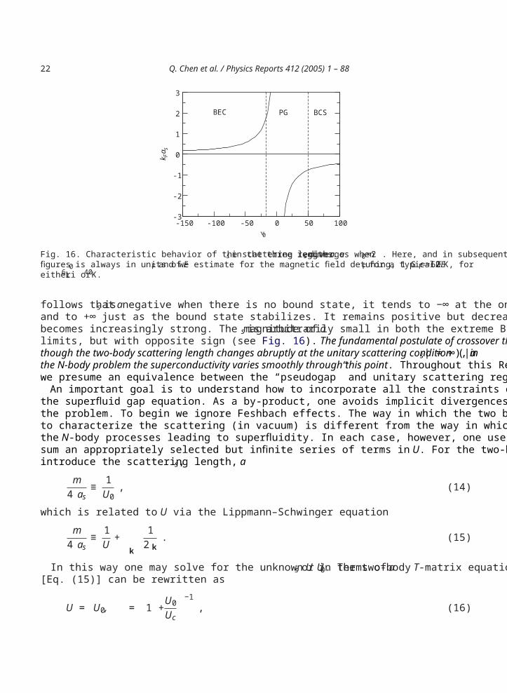
Fig. 16. Characteristic behavior of the scattering lengthas in the three regimes.as diverges when 0 =2 . Here, and in subsequentfigures 0 is always in units of EF and we estimate for the magnetic field detuning, 1 G ≈ 60EF for a typical EF = 2 K, foreither 6Li or 40K.
follows that as is negative when there is no bound state, it tends to −∞ at the onset of the bound stateand to +∞ just as the bound state stabilizes. It remains positive but decreases in value as the interactionbecomes increasingly strong. The magnitude of as is arbitrarily small in both the extreme BEC and BCSlimits, but with opposite sign (see Fig. 16). The fundamental postulate of crossover theory is that eventhough the two-body scattering length changes abruptly at the unitary scattering condition (|as|=∞ ), inthe N-body problem the superconductivity varies smoothly through this point. Throughout this Review,we presume an equivalence between the “pseudogap” and unitary scattering regimes.
An important goal is to understand how to incorporate all the constraints of the two body physics intothe superfluid gap equation. As a by-product, one avoids implicit divergences which would also appear inthe problem. To begin we ignore Feshbach effects. The way in which the two body interaction U entersto characterize the scattering (in vacuum) is different from the way in which it enters to characterizethe N-body processes leading to superfluidity. In each case, however, one uses a T-matrix formulation tosum an appropriately selected but infinite series of terms in U. For the two-body problem in vacuum, weintroduce the scattering length, as,
m4 as
≡ 1U0
, (14)
which is related to U via the Lippmann–Schwinger equation
m4 as
≡ 1U
+k
12 k
. (15)
In this way one may solve for the unknown U in terms of as or U0. The two-body T-matrix equation[Eq. (15)] can be rewritten as
U = U0, = 1 + U0
Uc
−1, (16)
Q. Chen et al. / Physics Reports 412 (2005) 1 – 88 23
where we define the quantity Uc as
U−1c = −
k
12 k
. (17)
Here Uc is the critical value of the potential associated with the binding of a two particle state in vacuum.Specific evaluation of Uc requires that there be a cut-off imposed on the above summation, associatedwith the range of the potential.
Now let us turn to the Feshbach problem, where the superfluidity is constrained by a more extendedset of parameters U, g, and also . Provided we redefine the appropriate “two body” scattering length,Eq. (15) holds even in the presence of Feshbach effects (Milstein et al., 2002; Ohashi and Griffin, 2002).It has been shown that U in the above equations is replaced by Ueff and as by a∗
s
m4 a∗
s≡ 1
Ueff+
k
12 k
. (18)
Here it is important to stress that many body effects, via the fermionic chemical potential enter into a∗s .
More precisely the effective interaction between two fermions is Q dependent. It arises from a secondorder process involving emission and absorption of a molecular boson. The net effect of the direct plusindirect interactions is given by
Ueff(Q) ≡ U + g2D0(Q) , (19)
where
D0(Q) ≡ 1/[ i n − mbq − + 2 ] (20)
is the noninteracting molecular boson propagator. What appears in the gap equation, however, is
Ueff(Q =0) ≡ Ueff = U − g2
− 2. (21)
Experimentally, the two body scattering lengtha∗s varies with magnetic field B. Near resonance, it can be
parameterized (Kokkelmans et al., 2002) in terms of three parameters of the two body problemU0, g0 andthe magnetic field which at resonance is given byB0. One fits the scattering length toabg(1−(w/(B−B 0))so that the width w is related to g0 and the background scattering length abg is related to U0. Away fromresonance, the crossover picture requires that the scattering length vanish asymptotically as
a∗s ≈ 0 in extreme BEC limit , (22)
so that the system represents an ideal Bose gas. Here it should be noted that this BEC limit corresponds to→ +. The counterpart of Eq. (22) also holds for the one channel problem. Note that the actual resonance
of the many body problem will be somewhat shifted from the atomic-fitted resonance parameter B0.It is convenient to define the parameter 0 which is directly related to the difference in the applied
magnetic field B and B0
0 = (B − B0) 0 , (23)

24 Q. Chen et al. / Physics Reports 412 (2005) 1 – 88
where 0 is the difference in the magnetic moment of the singlet and triplet paired states. We will usethe parameter 0 as a measure of magnetic field strength throughout this Review. The counterpart ofEq. (14) is then
m4 a∗
s≡ 1
U0 − g20
0−2
≡ 1U∗ , (24)
where U0 =4 abg/m and g20 =U0
0w. For the purposes of this Review we will use the scattering lengtha∗
s , although for simplicity we often drop the asterisk and write it as as.We can again invert the Lippmann–Schwinger or T-matrix scattering equation (Bruun and Pethick,
2004; Kokkelmans et al., 2002) to arrive at the appropriate parameters g and which enter into theHamiltonian and thus into the gap equation. Just as in Eq. (16), one finds a connection between measurableparameters (with subscript 0) and their counterparts in the Hamiltonian (without the subscript):
U = U0, g = g0, − 0 = − g20
Uc. (25)
To connect the various energy scales, which appear in the problem, typically 1G ≈ 60EF for both 6Liand 40K. Here it is assumed that the Fermi energy is EF ≈ 2 K.
In Fig. 16 and using Eq. (18), we plot a prototypical scattering length kFas ≡ kFa∗s as a function of
the magnetic field dependent parameter, 0. This figure indicates the BEC, BCS and PG regimes. Here,as earlier, the PG regime is bounded on the left by = 0 and on the right by (Tc) ≈ 0.
A key finding associated with this plot is that the PG regime begins on the so-called “BEC side ofresonance”, independent of whether Feshbach effects are included or not. That is, the fermionic chemicalpotential reaches zero while the scattering length is positive. This generic effect of the ground stateself consistent equations arises from the Pauli principle. For an isolated system, two particle resonantscattering occurs at U = Uc, where Uc is defined in Eq. (17). In the many body context, because ofPauli principle repulsion between fermions, it requires an effectively stronger attraction to bind particlesinto molecules. Stated alternatively, the onset of the fermionic regime ( >0) occurs for more stronglyattractive interactions, than those required for two body resonant scattering. As a consequence of >0,there is very little condensate weight in the Feshbach boson channel near the unitary limit, for values ofthe coupling parameter g0, appropriate to currently studied (and rather wide) Feshbach resonances.
Finally, it is useful to compare the two interaction terms which we have defined above, (Ueff andU∗), and to contrast their behavior in the BEC and unitary limits. The quantity U∗is proportional to thescattering length; it reflects the two body physics and necessarily diverges at unitarity, whereUeff =Uc. Bycontrast, in the BEC regime,U∗, or a∗
s approaches zero, (under the usual presumption that the interactionis a contact interaction). This vanishing ofU∗should be compared with the observation that the quantityUeff , which reflects the many body physics, must diverge in this BEC limit.
1.5.1. Differences between one and two channel models: physics of Feshbach bosonsThe main effects associated with including the explicit Feshbach resonance are twofold. These Feshbach
bosons provide a physical mechanism for tuning the scattering length to be arbitrarily large, and in theBEC limit, they lead to different physics from the one channel problem. As will be illustrated later viaa comparison of Figs. 23 and 25, in an artificial way one can capture most of the salient physics of theunitary regime via a one channel approach in which one drops all molecular boson related terms in the
Q. Chen et al. / Physics Reports 412 (2005) 1 – 88 25
Hamiltonian, but takes the interaction U to be arbitrary. In this way there is very little difference betweenfermion-only and fermion–boson models. There is an important proviso, though, that one is not dealingwith narrow resonances which behave rather differently near unitarity, as will be seen in Fig. 32. Inaddition, as in the one channel model a form of universality (Ho, 2004) is found in the ground state at theunitary limit, provided g is sufficiently large. This is discussed later in the context of Fig. 30.
We emphasize that, within the BEC regime there are three important effects associated with the Fes-hbach coupling g. As will become clear later, (i) in the extreme BEC limit when g is nonzero, thereare no occupied fermionic states. The number constraint can be satisfied entirely in terms of Feshbachbosons. (ii) The absence of fermions will, moreover, greatly weaken the inter-boson interactions whichare presumed to be mediated by the fermions. In addition, as one decreases |Ueff| from very attractive tomoderately attractive (i.e., increasesa∗
s on the BEC side) the nature of the condensed pairs changes. Evenin the absence of Feshbach bosons (FB), the size of the pairs increases. But in their presence the admix-ture of bosonic (i.e., molecular bosons) and fermionic (i.e., Cooper pair) components in the condensateis continuously varied from fully bosonic to fully fermionic. Finally (iii) the role of the condensate entersin two very different ways into the self consistent gap and number equations, depending on whether ornot there are FB. The molecular boson condensate appears principally in the number equation, while theCooper pair condensate appears principally in the gap equation. To make this point clearer we can referahead to Eq. (81) which contains the FB condensate contribution n0
b. By contrast the Cooper condensatecontribution sc enters into the total excitation gap as in Eq. (10) and is, in turn, constrained viaEq. (69). Points (i) and (iii), which may appear somewhat technical, have essential physical implications,among the most important of these is point (ii) above.
We stress, however, that for the PG and BCS regimes the differences with and without FB are, however,considerably less pronounced.
1.6. Current summary of cold atom experiments: crossover in the presence of Feshbach resonances
There has been an exciting string of developments over the past few years in studies of ultracoldfermionic atoms, in particular,6Li and 40K, which have been trapped and cooled via magnetic and opticalmeans. Typically these traps contain∼105 atoms at very low densities ≈1013 cm−3 when cooled to verylow T. Here the Fermi temperature EF in a trap can be estimated to be of the order of a micro-Kelvin.It was argued on the basis of BCS theory alone (Houbiers et al., 1997), and rather early on (1997), thatthe temperatures associated with the superfluid phases may be attainable in these trapped gases. Thisset off a search for the “holy grail” of fermionic superfluidity. That a Fermi degenerate state could bereached at all is itself quite remarkable; this was first reported by DeMarco and Jin (1999). By late2002 reports of unusual hydrodynamics in a degenerate Fermi gas indicated that strong interactions werepresent (O’Hara et al., 2002). This strongly interacting Fermi gas (associated with the unitary scatteringregime) has attracted widespread attention independent of the search for superfluidity, because it appearsto be a prototype for analogous systems in nuclear physics (Baker, 1999; Heiselberg, 2004a) and inquark–gluon plasmas (Itakura, 2003; Kolb and Heinz, 2003). Moreover, there has been a fairly extensivebody of analytic work on the ground state properties of this regime (Carlson et al., 1999; Heiselberg,2001), which goes beyond the simple mean field wave function ansatz.
As a consequence of attractive s-wave interactions between fermionic atoms in different hyperfinestates, it was anticipated that dimers could also be made. Indeed, these molecules formed rather efficiently(Cubizolles et al., 2003; Regal et al., 2003; Strecker et al., 2003) as reported in mid-2003 either via
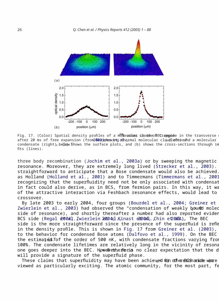
26 Q. Chen et al. / Physics Reports 412 (2005) 1 – 88
(a)
(b)
Fig. 17. (Color) Spatial density profiles of a molecular cloud of trapped40K atoms in the BEC regime in the transverse directionsafter 20 ms of free expansion (from Greiner et al., 2003), showing thermal molecular cloud above Tc (left) and a molecularcondensate (right) below Tc. (a) Shows the surface plots, and (b) shows the cross-sections through images (dots) with bimodalfits (lines).
three body recombination (Jochim et al., 2003a) or by sweeping the magnetic field across a Feshbachresonance. Moreover, they are extremely long lived (Strecker et al., 2003). From this work it was relativelystraightforward to anticipate that a Bose condensate would also be achieved. Credit goes to theorists suchas Holland (Holland et al., 2001) and to Timmermans (Timmermans et al., 2001) and their co-workers forrecognizing that the superfluidity need not be only associated with condensation of long lived bosons, butin fact could also derive, as in BCS, from fermion pairs. In this way, it was argued that a suitable tuningof the attractive interaction via Feshbach resonance effects, would lead to a realization of a BCS–BECcrossover.
By late 2003 to early 2004, four groups (Bourdel et al., 2004; Greiner et al., 2003; Jochim et al., 2003b;Zwierlein et al., 2003) had observed the “condensation of weakly bound molecules” (that is, on theas >0side of resonance), and shortly thereafter a number had also reported evidence for superfluidity on theBCS side (Regal et al., 2004; Zwierlein et al., 2004; Kinast et al., 2004; Chin et al., 2004). The BECside is the more straightforward since the presence of the superfluid is reflected in a bi-modal distributionin the density profile. This is shown in Fig. 17 from Greiner et al. (2003), and is conceptually similarto the behavior for condensed Bose atoms (Dalfovo et al., 1999). On the BEC side but near resonance,the estimated Tc is of the order of 500 nK, with condensate fractions varying from 20% or so, to nearly100%. The condensate lifetimes are relatively long in the vicinity of resonance, and fall off rapidly asone goes deeper into the BEC. However, for as <0 there is no clear expectation that the density profilewill provide a signature of the superfluid phase.
These claims that superfluidity may have been achieved on the BCS side ( as <0) of resonance wereviewed as particularly exciting. The atomic community, for the most part, felt the previous counterpart
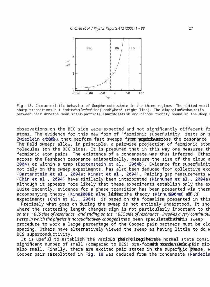
Q. Chen et al. / Physics Reports 412 (2005) 1 – 88 27
-150 -100 -50 0 50 100ν0
0
1
2
3
k F ξ
BEC PG BCS
Fig. 18. Characteristic behavior of Cooper pair size in the condensate in the three regimes. The dotted vertical lines are notsharp transitions but indicate where = 0 (left line) and where (Tc) ≈ 0 (right line). The dimensionless kF gives the ratiobetween pair size and the mean inter-particle spacing 1/kF. Pairs shrink and become tightly bound in the deep BEC regime.
observations on the BEC side were expected and not significantly different from condensation in Boseatoms. The evidence for this new form of “fermionic superfluidity” rests on studies (Regal et al., 2004;Zwierlein et al., 2004) that perform fast sweeps from negative as to positive as across the resonance.The field sweeps allow, in principle, a pairwise projection of fermionic atoms (on the BCS side) ontomolecules (on the BEC side). It is presumed that in this way one measures the momentum distribution offermionic atom pairs. The existence of a condensate was thus inferred. Other experiments which sweepacross the Feshbach resonance adiabatically, measure the size of the cloud after release (Bourdel et al.,2004) or within a trap (Bartenstein et al., 2004b). Evidence for superfluidity on the BCS side, which doesnot rely on the sweep experiments, has also been deduced from collective excitations of a fermionic gas(Bartenstein et al., 2004a; Kinast et al., 2004). Pairing gap measurements with radio frequency (RF) probes(Chin et al., 2004) have similarly been interpreted (Kinnunen et al., 2004a) as evidence for superfluidity,although it appears more likely that these experiments establish only the existence of fermionic pairs.Quite recently, evidence for a phase transition has been presented via thermodynamic measurements andaccompanying theory (Kinast et al., 2005). The latter, like the theory (Kinnunen et al., 2004a) of RFexperiments (Chin et al., 2004), is based on the formalism presented in this Review.
Precisely what goes on during the sweep is not entirely understood. It should be stressed again thatwhere the scattering length changes sign is not particularly important to the N-body physics. Thus startingon the “BCS side of resonance” and ending on the “BEC side of resonance” involves a very continuoussweep in which the physics is not qualitatively changed. It has been speculated that for this sweepprocedure to work a large percentage of the Cooper pair partners must be closer than the inter-atomicspacing. Others have alternatively viewed the sweep as having little to do with the large Cooper pairs ofBCS superconductivity.
It is useful to establish the various pair sizes here. In the PG regime the normal state consists of asignificant number of small (compared to BCS) pre-formed pairs. Below Tc, the condensate pair size isalso small. Finally, there are excited pair states in the superfluid phase, with characteristic size pg. TheCooper pair size as plotted in Fig. 18 was deduced from the condensate (Randeria, 1995) at T = 0,
28 Q. Chen et al. / Physics Reports 412 (2005) 1 – 88
but this can be shown to be rather similar to pg, corresponding to the size of excited pair states (Chen,2000; Chen et al., 1998) both above and below Tc. It seems plausible that during the sweep there issome rearrangement of excited states (both fermionic and bosonic) and condensate. In addition, all pairs(excited and condensate) contract in size. When, at the end of a sweep, they are sufficiently small, thenthey are more “visible”. What appears to be essential, however, is that the sweep time scales are rapidenough so that the existence of a condensate at the initial starting point is a necessary and sufficientcondition for observing a condensate at the end of a sweep.
1.7. T-matrix-based approaches to BCS–BEC crossover in the absence of Feshbach effects
In this subsection we introduce the concept of a T-matrix within the pairing channel. This is defined inEq. (26) below and it represents an effectively screened interaction in which the appropriate polarizability( ) is associated with the particle–particle rather than the particle–hole channel, as in the more conventionaldielectric susceptibility. The T-matrix thus appears as an infinite series of two particle “ladder” diagrams.
Away from zero temperature, a variety of different many body approaches have been invoked to addressthe physics of BCS–BEC crossover. For the most part, these revolve around T-matrix schemes. Here onesolves self consistently for the single fermion propagator (G) and the pair propagator (t). That one stopsat this level without introducing higher order Green’s functions (involving three, and four particles, etc)is believed to be adequate for addressing a leading order mean field theory such as that represented byEq. (1). One can see that pair–pair (boson–boson) interactions are only treated in a mean field averagingprocedure; they arise exclusively from the fermions and are presumed to be sufficiently weak so as notto lead to any incomplete condensation in the ground state, as is compatible with Eq. (1).
One can view this approach as the first step beyond BCS in a hierarchy of mean field theories. In BCS,above Tc one includes only the bare fermion propagatorG0. Below Tc, pairs play a role but only throughthe condensate. At the next level one accounts for the interaction between particles and noncondensedpairs in both the normal and superconducting states. The pairs introduce a self energy into the particles,which represents a correction to BCS theory. The pairs are treated at an effective mean field level. Bytruncating the equations of motion in this way, the effects of all higher order Green’s functions aresubsumed into t in an averaged way.
Below we demonstrate that at this T-matrix level there are a number of distinct schemes which can beimplemented to address BCS–BEC crossover physics. These same alternatives have also entered into adiscussion of pre-formed pairs as they appear in treatments of superconducting fluctuations. Above Tc,quite generally one writes for the T-matrix
t (Q) = U1 + U (Q)
(26)
and theories differ only on what is the nature of the pair susceptibility(Q), and the associated self energyof the fermions. Here and throughout we use Q to denote a four-vector and write Q ≡ T i n q,where n is a Matsubara frequency. Below Tc one can also consider a T-matrix approach to describe theparticles and pairs in the condensate. For the most part we will defer extensions to the broken symmetryphase to Section 2.2.
Q. Chen et al. / Physics Reports 412 (2005) 1 – 88 29
1.7.1. Review of BCS theory using the T-matrix approachIn order to assess alternative schemes, it is useful to review BCS theory within a T-matrix formalism.
In BCS theory, pairs explicitly enter into the problem below Tc, but only through the condensate. Thesecondensed pairs are associated with a T-matrix given by
tsc(Q) = − 2sc (Q)/T (27)
with fermionic self energy
sc(K) =Q
tsc(Q)G0(Q − K) (28)
so that sc(K) = − 2scG0(−K) . Here, and throughout, G0 is the Green’s function of the noninteracting
system. The number of fermions in a BCS superconductor is given by
n =2K
G(K) (29)
and
G(K) = [G−10 (K) − sc(K)]−1 (30)
Doing the Matsubara summation in Eq. (29), one can then deduce the usual BCS expression for thenumber of particles, which determines the fermionic chemical potential
n =k
1 − k −Ek
+ 2 k −Ek
f (Ek) , (31)
where
Ek = ( k − )2 + 2sc(T ) (32)
We need, however, an additional equation to determine sc(T ). The BCS gap equation can bewritten as
1 + U BCS(0) =0, T ⩽Tc , (33)
where
BCS(Q) =K
G(K)G 0(Q − K) . (34)
This suggests that one consider the uncondensed or normal state pair propagator to be of the form
t (Q) = U1 + U BCS(Q)
(35)
then in the superconducting state we have a BEC like condition on the pair chemical potential pairdefined by
t−1(Q =0) = pair × const . (36)
30 Q. Chen et al. / Physics Reports 412 (2005) 1 – 88
where the overall constant is unimportant for the present purposes. Thus we say that the pair chemicalpotential satisfies
pair = 0, T ⩽Tc . (37)
That pair vanishes at allT ⩽Tc is a stronger condition than the usual Thouless condition forTc. Moreover,it should be stressed that BCS theory is associated with a particular asymmetric form for the pairsusceptibility. These uncondensed pairs play virtually no role in BCS superconductors but the structureof this theory points to a particular choice for a pair susceptibility. We can then write the self consistentcondition on sc which follows from Eq. (33). Using Eqs. (27)–(34), we find the expected form for theBCS gap equation. This represents a constraint on the order parameter sc:
sc(T ) = −Uk
sc(T )1 − 2f (Ek)2Ek
. (38)
The above discussion was presented in a somewhat different way in a paper by Kadanoff andMartin (1961).
1.7.2. Three choices for the T-matrix of the normal state: problems with the Nozieres Schmitt-Rinkapproach
On general grounds we can say that there are three obvious choices for (Q) which appears in thegeneral definition of the T-matrix in Eq. (26). Each of these has been studied rather extensively in theliterature. All of these introduce corrections to BCS theory and all were motivated by attempts to extendthe crossover ground state to finite T, or to understand widespread pseudogap effects in the high Tcsuperconductors. In analogy with Gaussian fluctuations, one can consider
0(Q) =K
G0(K)G 0(Q − K) (39)
with self energy
0(K) =Q
t (Q)G0(Q − K) , (40)
which appears in G in the analogue of Eq. (30). The number equation is then deduced by using Eq. (29).This scheme was adopted by Nozieres and Schmitt-Rink (NSR), although these authors (Nozières
and Schmitt-Rink, 1985; Randeria, 1995) approximated the number equation (Serene, 1989) by using aleading order series for G in Eq. (30) with
G = G0 + G0 0G0 . (41)
It is straightforward, however, to avoid this approximation in Dyson’s equation, and a number of groups(Jankó et al., 1997; Pieri et al., 2004) have extended NSR in this way.
Similarly one can consider
(Q) =K
G(K)G(Q − K) (42)
Q. Chen et al. / Physics Reports 412 (2005) 1 – 88 31
with self energy
¯(K) =Q
t (Q)G(Q − K). (43)
This latter scheme (sometimes known as fluctuation-exchange or FLEX) has been also extensively dis-cussed in the literature, by among others, Haussmann (1993), Tchernyshyov (1997), Micnas et al. (1995)and Yanase et al. (2003).
Finally, we can contemplate the asymmetric form (Chen et al., 1998; Giovannini and Berthod, 2001)for the T-matrix, so that the coupled equations for t (Q)and G(K) are based on
(Q) =K
G(K)G 0(Q − K) (44)
with self energy
(K) =Q
t (Q)G0(Q − K) . (45)
Each of these three schemes determines the superfluid transition temperature via the Thouless condition.Thus pair = 0 leads to a slightly different expression for Tc, based on the differences in the choice ofT-matrix which appears in Eq. (36).
A central problem with the NSR scheme ( ≈ G0G0) is that it incorporates self energy effects onlythrough the number equation. The absence of self energy effects in the gap equation is equivalent to thestatement that pseudogap effects only indirectly affect Tc: the particles acquire a self energy from thepairs but these self energy effects are not fed back into the propagator for the pairs. On physical groundsone anticipates that the pseudogap must have a direct effect on Tc as a consequence of the associatedreduction in the density of states. Other problems related to the thermodynamics were pointed out (Sofoand Balseiro, 1992) when NSR was applied to a two dimensional system. Finally, because only the numberequation contains self energy effects, it is not clear if one can arrive at a proper vanishing of the superfluiddensity s at Tc within this approach. This requires a precise cancellation between the diamagnetic currentcontributions (which depend on the number equation) and the paramagnetic terms (which reflect the gapequation).
One might be inclined, then, to prefer (Serene, 1989) the FLEX (≈ GG) scheme since it is -derivable,in the sense of Baym (1962). This means that it is possible to write down a closed form expression for thethermodynamical potential, from which one derives other physical quantities via functional derivatives ofthis potential. Theoretical consistency issues in this approach have been rather exhaustively discussed byHaussmann (1993) aboveTc. We are not aware of a fully self consistent calculation of s below Tc, at thesame level of completeness as Haussmann’s normal state analysis (or, for that matter, of the counterpartdiscussion to Section 3.1 and accompanying Appendix B). However, in principle, it should be possible toarrive at a proper expression for the superfluid density, providing Ward identities are imposed. There issome ambiguity (Benard et al., 1993; Micnas et al., 1995; Tchernyshyov, 1997) about whether pseudogapeffects are present in the FLEX approach; a consensus has not been reached at this time. Numerical workbased on FLEX is more extensive (Benard et al., 1993; Deisz et al., 1998) than for the other two alternativeschemes.
It will be made clear in what follows that, if one’s goal is to extend the usual crossover ground stateof Eq. (1) to finite temperatures, then one must choose the asymmetric form for the pair susceptibility.
32 Q. Chen et al. / Physics Reports 412 (2005) 1 – 88
Here ≈ GG0. This is different from the approach of Nozieres and Schmitt-Rink in which there is noevident consistency between their finite T treatment and the presumed ground state. Some have claimed(Randeria, 1995) that an NSR-based approach, when extended below Tc, reproduces Eqs. (69) and (70).But elsewhere in the literature it has been shown that these ground state self consistency conditions arederived from a lower level theory (Kostyrko and Ranninger, 1996). They arise from aT =0 limit of whatis called the saddle point approximation, or mean field approach. When pairing fluctuations beyond thesaddle point (Nozières and Schmitt-Rink, 1985) are included, the number equation is changed. Then theground state is no longer that of Eq. (1) (Pieri et al., 2004). In the cold atom literature, the distinctionbetween the NSR-extrapolated ground state and the ground state of Eq. (1) has been pointed out in thecontext of atomic density profiles (Perali et al., 2004b) within traps.
It should be evident from Eq. (34) and the surrounding discussion that the asymmetric form is uniquelyassociated with the BCS-like behavior implicit in Eq. (1). The other two T-matrix approaches lead todifferent ground states which should, however, be very interesting in their own right. These will need tobe characterized in future.
Additional support for the asymmetric form, which will be advocated here, was provided by Kadanoffand Martin. In their famous paper they noted that several people had surmised that the form for (Q)involving GG would be more accurate. However, as claimed in (Kadanoff and Martin, 1961), “Thissurmise is not correct.” Aside from theoretical counter-arguments which they present, the more symmetriccombination of Green’s functions “can also be rejected experimentally since they give rise to aT 2 specificheat.” Similar arguments in support of the asymmetric form were introduced (Hassing and Wilkins, 1973)into the literature in the context of addressing specific heat jumps.
1.8. Superconducting fluctuations: a type of pre-formed pairs
While there are no indications of bosonic degrees of freedom, (other than in the condensate), withinstrict BCS theory, it has been possible to access these bosons via probes of superconducting fluctuations.Quasi-one dimensional, or quasi-2D superconductors in the presence of significant disorder exhibit fluc-tuation effects (Larkin and Varlamov, 2001) or precursor pairing as seen in “paraconductivity”, fluctuationdiamagnetism, as well as other unusual behavior, often consisting of divergent contributions to transport.One frequently computes (Kwon and Dorsey, 1999) these bosonic contributions to transport by use of atime dependent Ginzburg Landau (TDGL) equation of motion. This is rather similar to a Gross Pitaevskiiformalism except that the “bosons” here are highly damped by the fermions.
Alternatively T-matrix based approaches (involving all three choices of (Q)) have been extensivelyused to discuss conventional superconducting fluctuations. The advantage of these latter schemes is thatone can address both the anomalous bosonic and fermionic contributions to transport through the famousAslamazov–Larkin and Maki–Thompson diagrams (Larkin and Varlamov, 2001). We defer a discussionof these issues until Appendix B.
It is useful to demonstrate first how conventional superconducting fluctuations behave at the lowestlevel of self consistency, called the Hartree approximation. This scheme is closely associated (Stajicet al., 2003a) with a GG0 T-matrix, as is discussed in more detail in Appendix C. It is also closelyassociated with BCS theory, for one can show that, in the spirit of Eq. (1), at this Hartree level theexcitation gap (Tc) and Tc lie on a specific BCS curve (specified by n and U). What is different fromstrict BCS theory is that the onset of superconductivity takes place in the presence of a finite excitation gap(i.e., pseudogap), just as shown in Fig. 3. This, then, reflects the fact that there are pre-formed pairs atTc.
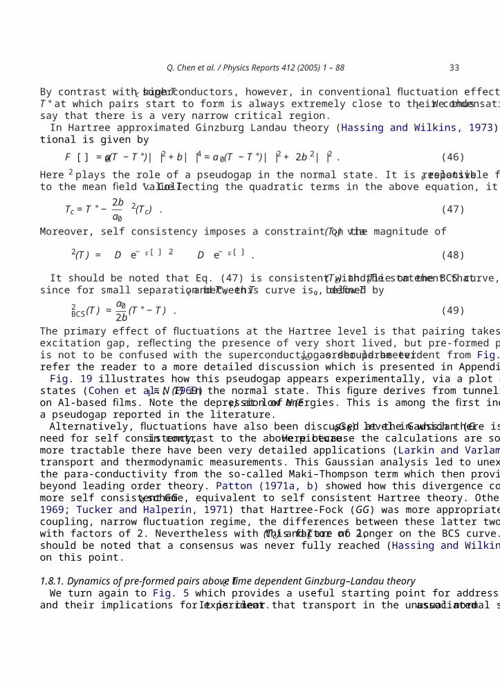
Q. Chen et al. / Physics Reports 412 (2005) 1 – 88 33
By contrast with high Tc superconductors, however, in conventional fluctuation effects, the temperatureT∗at which pairs start to form is always extremely close to their condensation temperature Tc. We thussay that there is a very narrow critical region.
In Hartree approximated Ginzburg Landau theory (Hassing and Wilkins, 1973) the free energy func-tional is given by
F [ ] = a0(T − T∗)| |2 + b| |4 ≈ a0(T − T∗)| |2 + 2b 2| |2 . (46)
Here 2 plays the role of a pseudogap in the normal state. It is responsible for a lowering of Tc relativeto the mean field value T∗. Collecting the quadratic terms in the above equation, it follows that
Tc = T∗− 2ba0
2(Tc) . (47)
Moreover, self consistency imposes a constraint on the magnitude of (Tc) via
2(T ) = D e− F[ ] 2 D e− F[ ] . (48)
It should be noted that Eq. (47) is consistent with the statement that (Tc) and Tc lie on the BCS curve,since for small separation between Tc and T∗, this curve is, below Tc, defined by
2BCS(T ) ≈a0
2b(T∗− T ). (49)
The primary effect of fluctuations at the Hartree level is that pairing takes place in the presence of a finiteexcitation gap, reflecting the presence of very short lived, but pre-formed pairs. It should be clear thatis not to be confused with the superconducting order parameter sc, as should be evident from Fig. 3. Werefer the reader to a more detailed discussion which is presented in Appendix C.
Fig. 19 illustrates how this pseudogap appears experimentally, via a plot of the normalized density ofstates (Cohen et al., 1969) 1 ≡ N(E) in the normal state. This figure derives from tunneling measurementson Al-based films. Note the depression of N(E F) at low energies. This is among the first indications fora pseudogap reported in the literature.
Alternatively, fluctuations have also been discussed at the Gaussian (G0G0) level in which there is noneed for self consistency, in contrast to the above picture. Here because the calculations are so muchmore tractable there have been very detailed applications (Larkin and Varlamov, 2001) of essentially alltransport and thermodynamic measurements. This Gaussian analysis led to unexpected divergences inthe para-conductivity from the so-called Maki–Thompson term which then provided a motivation to gobeyond leading order theory. Patton (1971a, b) showed how this divergence could be removed within amore self consistent GG0 scheme, equivalent to self consistent Hartree theory. Others argued (Schmid,1969; Tucker and Halperin, 1971) that Hartree-Fock (GG) was more appropriate, although in this weakcoupling, narrow fluctuation regime, the differences between these latter two schemes are only associatedwith factors of 2. Nevertheless with this factor of 2, (Tc) and Tc are no longer on the BCS curve. Itshould be noted that a consensus was never fully reached (Hassing and Wilkins, 1973) by the communityon this point.
1.8.1. Dynamics of pre-formed pairs above Tc: time dependent Ginzburg–Landau theoryWe turn again to Fig. 5 which provides a useful starting point for addressing bosonic degrees of freedom
and their implications for experiment. It is clear that transport in the unusual normal state, associated
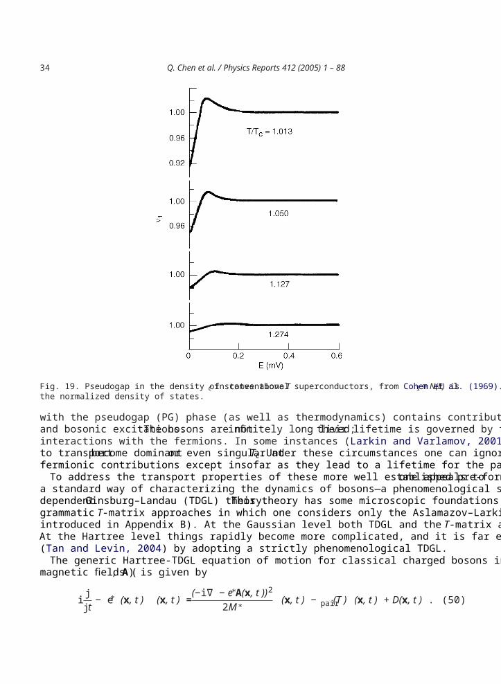
34 Q. Chen et al. / Physics Reports 412 (2005) 1 – 88
Fig. 19. Pseudogap in the density of states above Tc in conventional superconductors, from Cohen et al. (1969). 1 ≡ N(E) isthe normalized density of states.
with the pseudogap (PG) phase (as well as thermodynamics) contains contributions from both fermionicand bosonic excitations. The bosons are not infinitely long lived; their lifetime is governed by theirinteractions with the fermions. In some instances (Larkin and Varlamov, 2001), the bosonic contributionsto transport become dominant or even singular at Tc. Under these circumstances one can ignore thefermionic contributions except insofar as they lead to a lifetime for the pairs.
To address the transport properties of these more well established pre-formed pairs, one appeals toa standard way of characterizing the dynamics of bosons—a phenomenological scheme known as timedependent Ginsburg–Landau (TDGL) theory. This theory has some microscopic foundations in dia-grammatic T-matrix approaches in which one considers only the Aslamazov–Larkin terms (which areintroduced in Appendix B). At the Gaussian level both TDGL and the T-matrix approaches are tractable.At the Hartree level things rapidly become more complicated, and it is far easier to approach the problem(Tan and Levin, 2004) by adopting a strictly phenomenological TDGL.
The generic Hartree-TDGL equation of motion for classical charged bosons interacting with electro-magnetic fields ( , A) is given by
ijj t
− e∗ (x, t ) (x, t ) =(−i∇ − e∗A(x, t ))2
2M∗ (x, t ) −pair(T ) (x, t) + D(x, t ). (50)
Q. Chen et al. / Physics Reports 412 (2005) 1 – 88 35
Here (x, t )is a classical field variable representing the bosons which have vanishing chemical potentialpair at Tc. The function D(x, t )introduces a noise variable into the equation of motion. Generally is
complex.We will explore the implications of this equation in our more quantitative discussion of Section 6.5.
2. Quantitative details of crossover
2.1. T = 0, BEC limit without Feshbach bosons
We begin by reviewingT =0 crossover theory in the BEC limit. Our starting point is the ground statewavefunction 0 of Eq. (1), along with the self consistency conditions of Eq. (2). For positive chemicalpotential , the quantity sc(0) also corresponds to the energy gap for fermionic excitations. In the groundstate the two energy scales (0) and sc(0) are degenerate, just as they are (at all temperatures) in strictBCS theory.
It is convenient to rewrite these equations5 in terms of the inter-fermion scattering length as
m4 as
=k
12 k
− 12Ek
, (51)
n =k
1 − k −Ek
, T = 0 . (52)
In the fermionic regime ( >0) these equations are essentially equivalent to those of BCS theory, althoughat weak coupling appropriate to strict BCS, little attention is paid to the number equation since = EF isalways satisfied. The more interesting regime corresponds to ⩽ 0 where these equations take on a newinterpretation. Deep inside the BEC regime it can be seen that
n = 2sc(0) m2
4√
2m| | , (53)
which, in conjunction with Eq. (51) (expanded in powers of 2sc(0)/ 2):
m4 as
= (2m)3/2√ | |8
1 + 116
2sc(0)
2 , (54)
yields
= − 12ma2
s+ as n
m. (55)
5 To make the equations simpler, in much of what we present in this review we will consider a contact potential interaction.The momentum sums are assumed to run to infinity. More generally, one can include a cutoff function k for the momentumintegrals. The gap function thus becomes k = k . For the cuprate d-wave cuprate superconductors, k =cos kxa −cos kya.For our numerical work on atomic gases we use a Gaussian cutoff 2
k = e−k2/k 20 with k0 taken to be as large as is numerically
feasible.
36 Q. Chen et al. / Physics Reports 412 (2005) 1 – 88
This last equation is equivalent (Perali et al., 2003; Viverit et al., 2004) to its counterpart inGross–Pitaevskii (GP) theory. This theory describes true bosons, and is associated with the well knownequation of state
npairs = mB
4 aBB . (56)
To see the equivalence we associate the number of bosons npairs = n/2, the boson mass mB = 2mandthe bosonic scattering length aB = 2as. Here the bosonic chemical potential B = 2 + 0 and we define0 =1/(2ma2
s). This factor of 2 inaB/as has received a fair amount of attention in the literature. Althoughit will be discussed later in the Review, it should be noted now that this particular numerical valueis particular to the one channel description (Stajic et al., 2005b), and different from what is observedexperimentally (Petrov et al., 2004).
Despite these similarities with GP theory, the fundamental parameters are the fermionic sc(0) andchemical potential . It can be shown that in this deep BEC regime the number of pairs is directlyproportional to the superconducting order parameter
npairs = n2
= Z02sc(0) (57)
where
Z0 ≈ m2as8
. (58)
One may note from Eq. (57) that the “gap equation” now corresponds to a number equation (for bosons).Similarly the number equation, or constraint on the fermionic chemical potential defines the excitationgap for fermions, once the chemical potential is negative. In this way the roles of the two constraints areinverted (Randeria, 1995) relative to the BCS regime.
That a Gross–Pitaevskii approach captures the leading order physics at T = 0 can also be simply seenby rewriting the ground state wavefunction, as pointed out by Randeria (1995). Define vk/uk ≡ k,
0 = const k(1 + kc†kc
†−k)|0
=const expk
kc†kc
†−k |0 . (59)
Projecting onto a state with fixed particle number N yields
0 = constk
kc†kc
†−k
N/ 2
|0 . (60)
This is a GP wavefunction of composite bosons with the important proviso: that the characteristic sizeassociated with the internal wavefunction k is smaller than the inter-particle spacing. It should bestressed that, except in the BEC asymptotic limit, (where the “bosons” are noninteracting) there areessential differences between Eq. (60) and the Gross Pitaevskii wavefunction. Away from this extremelimit, pair-pair interactions (arising indirectly via the fermions and the Pauli principle), as well as thefinite size of the pairs, will differentiate this system from that of true interacting bosons. This same issuearises more concretely in the context of the collective mode spectrum of ultracold gases, as discussed inSection 5.3.
Q. Chen et al. / Physics Reports 412 (2005) 1 – 88 37
2.2. Extending conventional crossover ground state to T = 0: BEC limit without Feshbach bosons
How do we extend (Chen et al., 1998) this picture to finite T? In the BEC limit, as shown in Fig. 4, fermionpairs are well established or “pre-formed” within the entire range of superconducting temperatures. Thefundamental constraint associated with the BEC regime is that: for all T ⩽Tc, there should, thus, be notemperature dependence in fermionic energy scales. In this way Eqs. (51) and (52) must be imposed atall temperatures T.
m4 as
=k
12 k
− 12Ek
, (61)
n =k
1 − k −Ek
, T ⩽Tc . (62)
It follows that the number of pairs at T = 0 should be equal to the number of pairs at T = Tc.However, all pairs are condensed at T = 0. Clearly, the character of these pairs changes so that at Tc, allpairs are noncondensed. To implement these physical constraints (and to anticipate the results of a moremicroscopic theory) we write
npairs = n2
= Z02 (63)
npairs = ncondensedpairs (T ) + nnoncondensed
pairs (T ) (64)
so that we may decompose the excitation gap into two contributions2 = 2
sc(T ) + 2pg(T ) (65)
where sc(T )corresponds to condensed and pg(T )to the noncondensed gap component. Each of theseare proportional to the respective number of condensed and noncondensed pairs with proportionalityconstant Z0. At Tc,
nnoncondensedpairs = n
2=
qb( q, Tc) , (66)
where b(x) is the usual Bose–Einstein function and q is the unknown dispersion of the noncondensedpairs. Thus
2pg(Tc) = Z−1
0 b( q, Tc) =n2
Z−10 . (67)
We may deduce directly from Eq. (67) that 2pg = − Q t (Q), if we presume that below Tc, the noncon-
densed pairs have propagator
t (Q) = Z−10
− q. (68)
It is important to stress that the dispersion of the pairs q cannot be put in by hand. It is not knowna priori. Rather, it has be to derived according to the constraints imposed by Eqs. (61) and (62). We can
38 Q. Chen et al. / Physics Reports 412 (2005) 1 – 88
only arrive at an evaluation of q after establishing the nature of the appropriate T-matrix theory. In whatfollows we derive this dispersion using the two channel model. We state the one channel results here forcompleteness. In the absence of FB, q ≡ B0q2, where B0 ≡ 1/(2M∗
0 ). As a consequence of a “bosonic”self energy, which arises from fermion–boson (as distinguished from boson-boson) interactions, thebosonic dispersion is found to be quadratic. This quadratic dependence persists for the two channel caseas well.
2.3. Extending conventional crossover ground state to T = 0: T-matrix scheme in the presence ofFeshbach bosons
To arrive at the pair dispersion for the noncondensed pairs, q, we need to formulate a generalizedT-matrix based scheme which is consistent with the ground state conditions, and with the T dependenceof strict BCS theory. It is useful from a pedagogical point to now include the effects of Feshbach bosons(Stajic et al., 2004). Our intuition concerning how true bosons condense is much better than our intuitionconcerning the condensation of fermion pairs, except in the very limited BCS regime. We may assume that
and evolve with temperature in such a way as to be compatible with both the temperature dependencesof BCS and with the above discussion for the BEC limit. We thus take
(T ) = −Ueffk
(T )1 − 2f (Ek)2Ek
, (69)
n =k
1 − k −Ek
+ 2 k −Ek
f (Ek) , (70)
where Ek = ( k − )2 + 2(T ). Note that in the presence of Feshbach bosons, we use n to denote thedensity of fermionic atoms which is to be distinguished from the constituents of the Feshbach bosons.The total density of particles will be denoted by ntot. Eqs. (69) and (70) will play a central role in thisreview. They have been frequently invoked in the literature, albeit under the presumption that there is nodistinction between (T )and sc(T ).
Alternatively one can rewrite Eq. (69) as
m4 a∗
s=
k
12 k
− 1 − 2f (Ek)2Ek
. (71)
Clearly Eqs. (69) and (70) are consistent with Eqs. (61) and (62) since Fermi functions are effectivelyzero in the BEC limit. Our task is to find a T-matrix formalism which is compatible with (69) and (70),and to do this we focus first on the noncondensed molecular bosons. Their propagator may be written as
D(Q) ≡ 1i n − mb
q − + 2 − B(Q) . (72)
We presume that the self energy of these molecules can be written in the form
B(Q) ≡ −g2 (Q)/[1 + U (Q)] , (73)
where (Q) is as yet unspecified. This RPA-like self energy arises from interactions between the molecularbosons and the fermion pairs, and this particular form is required for self-consistency.
Q. Chen et al. / Physics Reports 412 (2005) 1 – 88 39
Noncondensed bosons in equilibrium with a condensate must necessarily have zero chemical potential.
boson(T ) =0, T ⩽Tc . (74)
This is equivalent to the Hugenholtz–Pines condition that
D−1(0) =0, T ⩽Tc . (75)
Using Eqs. (73) and (75) it can be seen that
U−1eff (0) + (0) =0, T ⩽Tc . (76)
This equation can be made compatible with our fundamental constraint in Eq. (69) provided we take
(Q) =K
G(K)G 0(Q − K) , (77)
where G(K)
G(K) ≡ [G−10 (K) − (K)]−1 (78)
includes a self energy given by the BCS-form
(K) = −G0(−K) 2 , (79)
which now involves the quantity to be distinguished from the order parameter sc. Note that with thisform for (K) , the number of fermions is indeed given by Eq. (70).
More generally, we may write the constraint on the total number of particles as follows. The numberof noncondensed molecular bosons is given directly by
nb(T ) = −Q
D(Q) . (80)
For T ⩽Tc, the number of fermions is given via Eq. (70). The total number (ntot) of particles is then
n +2nb + 2n0b = ntot , (81)
where n0b = 2
m is the number of molecular bosons in the condensate, and m is the order parameter forthe molecular condensate.
Thus far, we have shown that the condition that noncondensed molecular bosons have zero chemicalpotential, can be made consistent with Eqs. (69) and (70) provided we constrain(Q) and (K) as above.We now want to examine the counterpart condition on the fermions and their condensate contribution.The analysis leading up to this point should make it clear that we have both condensed and noncondensedfermion pairs, just as we have both condensed and noncondensed molecular bosons. Moreover, thesefermion pairs and Feshbach bosons are strongly admixed, except in the very extreme BCS and BEC limits.Because of noncondensed pairs, we will see that the excitation gap is distinct from the superconductingorder parameter, although in the literature this distinction has not been widely recognized.
Just as the noncondensed molecular bosons have zero chemical potential below Tc we have the sameconstraint on the noncondensed fermion pairs which are in chemical equilibrium with the noncondensedbosons
pair = 0, T ⩽Tc . (82)
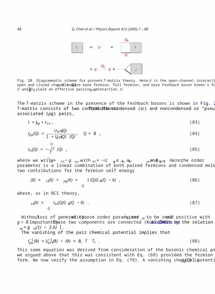
40 Q. Chen et al. / Physics Reports 412 (2005) 1 – 88
Fig. 20. Diagrammatic scheme for present T-matrix theory. Here U is the open-channel interaction, g is the coupling betweenopen and closed channels.G0, G andD0 are bare fermion, full fermion, and bare Feshbach boson Green’s functions, respectively.U and g2
0D0 yield an effective pairing interaction,Ueff .
The T-matrix scheme in the presence of the Feshbach bosons is shown in Fig. 20. Quite generally, theT-matrix consists of two contributions: from the condensed (sc) and noncondensed or “pseudogap”-associated (pg) pairs,
t = tpg + tsc , (83)
tpg(Q) = Ueff(Q)1 + Ueff(Q) (Q)
, Q = 0 , (84)
tsc(Q) = −˜2
scT
(Q) , (85)
where we write ˜sc = sc − g m, with sc = −U k a −k↓ak↑ and m = b q=0 . Here, the orderparameter is a linear combination of both paired fermions and condensed molecules. Similarly, we havetwo contributions for the fermion self energy
(K) = sc(K) + pg(K) =Q
t (Q)G0(Q − K) , (86)
where, as in BCS theory,
sc(K) =Q
tsc(Q)G0(Q − K) . (87)
Without loss of generality, we choose order parameters ˜sc and m to be real and positive withg <0. Importantly, these two components are connected (Kokkelmans et al., 2002) by the relation
m= g sc/[( − 2 )U ].The vanishing of the pair chemical potential implies that
t−1pg (0) = U−1
eff (0) + (0) =0, T ⩽Tc . (88)
This same equation was derived from consideration of the bosonic chemical potential. Most importantly,we argued above that this was consistent with Eq. (69) provided the fermion self energy assumes the BCSform. We now verify the assumption in Eq. (79). A vanishing chemical potential means that tpg(Q) is
Q. Chen et al. / Physics Reports 412 (2005) 1 – 88 41
strongly peaked around Q =0. Thus, we may approximate (Maly et al., 1999a) Eq. (86) to yield
(K) ≈ −G0(−K) 2 , (89)
where2(T ) ≡˜2
sc(T ) + 2pg(T ) , (90)
and we define the pseudogap pg
2pg ≡ −
Q=0
tpg(Q) . (91)
This bears a close resemblance to Eq. (80), if we write the number of noncondensed fermion pairs andmolecular bosons as
np(T ) = Z 2pg(T ) . (92)
Note that in the normal state (where pair is nonzero) one cannot make the approximation of Eq. (89).Referring back to our discussion of Hartree-approximated TDGL, a strong analogy between Eqs. (91)and (48) should be observed. There is a similar analogy between Eqs. (69) and (49); more details areprovided in Appendix C. We thus have that Eqs. (51) and (89) with Eq. (78) are alternative ways of writingEqs. (69) and (70). Along with Eq. (91) we now have a closed set of equations for addressing the orderedphase. Moreover the propagator for noncondensed pairs can now be quantified, using the self consistentlydetermined pair susceptibility. At moderately strong coupling and at small four-vector Q, we may expandto obtain
tpg(Q) = Z−1
− q + pair + i Q, (93)
Consequently, one can rewrite Eq. (91) as2pg(T ) = Z−1 b( q, T ). (94)
Here we introduce a simple notation for the small Q expansions:
(Q) − (0) = Z0(i n − B0q2) ,
U−1eff (Q) − U−1
eff (0) = Zg(i n − Bgq2)
with
Z0 = 12 2 n −2
kf ( k − ) ,
Zg = g2
[(2 − )U + g2]2 .
We have that Z = Z0 + Zg, Zb = (Z0 + Zg)/Z 0, and the q2 coefficient B ≡ 1/(2M∗) in q ≡ Bq2 issuch that
B = B0Z0 + 1/2MZ gZ .
42 Q. Chen et al. / Physics Reports 412 (2005) 1 – 88
The strong hybridization between the molecular bosons and fermion pairs should be stressed. Indeed,there is just one branch q for bosonic-like excitations, so that at small Q
D(Q) = Z−1b
− q + boson + i Q, (95)
where below Tc, pair = boson = 0. Here Q contains all the imaginary parts of the inverse T-matrixand it vanishes rapidly as Q → 0. As the coupling is decreased from the BEC limit towards BCS,the character of the pairs changes from pre-dominantly molecular-boson like to (noncondensed) Cooperpairs, composed only of the fermionic atoms.
2.4. Nature of the pair dispersion: size and lifetime of noncondensed pairs below Tc
We may rewrite the pair susceptibility (Chen et al., 1998, 1999) of Eq. (77) (after performing theMatsubara sum and analytically continuing to the real axis) in a relatively simple form as
(Q) =k
1 − f (Ek) − f ( k−q)Ek + k−q − − i0+ u2
k − f (Ek) − f ( k−q)Ek − k−q + + i0+v2
k , (96)
where u2k and v2
k are given by their usual BCS expressions in terms of and k ≡ k − . In the longwavelength, low frequency limit, the inverse of tpg can be written as
a12 + Z0 − q2
2M∗+ pair + i Q . (97)
We are interested in the moderate and strong coupling cases, where we can drop the a12 term in Eq.
(97), and hence we have Eq. (93) with
q ≡ q2
2M∗= q2 2pg
Z0. (98)
This establishes a quadratic dispersion and defines the effective pair mass,M∗. Analytical expressions forthis mass are possible via a small q expansion of , in Eq. (96). It is important to note that the pair massreflects the effective size pgof noncondensed pairs. This serves to emphasize the fact that theq2 dispersionderives from the compositeness of the “bosons”, in the sense of their finite spatial extent. A descriptionof the system away from the BEC limit must accommodate the fact that the pairs have an underlyingfermionic character. This pair mass has a different origin from the mass renormalization associated withreal interacting bosons. There one finds a mass shift which comes from a Hartree approximate treatmentof their q-dependent interactions. Finally, we note that pg is comparable to the size of pairs in thecondensate. In the weak coupling BCS limit, a small Q expansion of 0 shows that, because the leadingorder term in is purely imaginary, the 2 contribution cannot be neglected. The T-matrix, then, doesnot have the propagating q2 dispersion, discussed above.
It follows from Eq. (96) that the pair lifetime
Q =Z0 k
[1 − f (Ek) − f ( k−q)]u2k (Ek + k−q − )
+ [f (Ek) − f ( k−q)]v2k (Ek − k−q + ) . (99)
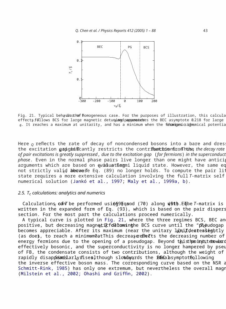
Q. Chen et al. / Physics Reports 412 (2005) 1 – 88 43
-300 -200 -100 0 100 200ν0/EF
0
0.1
0.2
0.3
T c /T
F
BEC PG BCS
Fig. 21. Typical behavior of Tc in the homogeneous case. For the purposes of illustration, this calculation includes Feshbacheffects. Tc follows BCS for large magnetic detuning parameter 0 and approaches the BEC asymptote 0.218 for large negative0. It reaches a maximum at unitarity, and has a minimum when the fermionic chemical potential changes sign.
Here Q reflects the rate of decay of noncondensed bosons into a bare and dressed fermion. Note thatthe excitation gap in Ek significantly restricts the contribution from the functions. Thus, the decay rateof pair excitations is greatly suppressed, due to the excitation gap (for fermions) in the superconductingphase. Even in the normal phase pairs live longer than one might have anticipated from “Pauli blocking”arguments which are based on evaluating Q in a Fermi liquid state. However, the same equations arenot strictly valid above Tc, because Eq. (89) no longer holds. To compute the pair lifetime in the normalstate requires a more extensive calculation involving the full T-matrix self consistent equations and theirnumerical solution (Jankó et al., 1997; Maly et al., 1999a, b).
2.5. Tc calculations: analytics and numerics
Calculations of Tc can be performed using Eqs. (69) and (70) along with Eq. (91). The T-matrix iswritten in the expanded form of Eq. (93), which is based on the pair dispersion as derived in the previoussection. For the most part the calculations proceed numerically.
A typical curve is plotted in Fig. 21, where the three regimes BCS, BEC and PG are indicated. Forpositive, but decreasing magnetic detuning 0, Tc follows the BCS curve until the “pseudogap” or (Tc)becomes appreciable. After its maximum (near the unitary limit, at slightly negative 0), Tc decreases,(as does ), to reach a minimum at ≈ 0. This decrease in Tc reflects the decreasing number of lowenergy fermions due to the opening of a pseudogap. Beyond this point, towards negative0, the system iseffectively bosonic, and the superconductivity is no longer hampered by pseudogap effects. In the presenceof FB, the condensate consists of two contributions, although the weight of the fermion pair componentrapidly disappears. Similarly Tc rises, although slowly, towards the ideal BEC asymptote, followingthe inverse effective boson mass. The corresponding curve based on the NSR approach (Nozières andSchmitt-Rink, 1985) has only one extremum, but nevertheless the overall magnitudes are not so different(Milstein et al., 2002; Ohashi and Griffin, 2002).
44 Q. Chen et al. / Physics Reports 412 (2005) 1 – 88
Analytic results are obtainable in the near-BEC limit only. The general expression for the effectivemass 1/M ∗
0 in this limit is given by
1M∗
0= 1
Z02
k
1m
v2k − 4Ekk2
3m2 2 v4k , (100)
where here FB effects have been dropped for simplicity. In what follows, we expand Eq. (100) in powersof na3
s and obtain after some algebra
M∗0 ≈ 2m 1 + a3
sn2
. (101)
We now invoke an important constraint, derived earlier in Eq. (66) which corresponds to the fact that atTc all fermions are constituents of uncondensed pairs
n2
=q
b( q, Tc) . (102)
From the above equation it follows that (M∗Tc)3/2 ∝ n = const. which, in conjunction with Eq. (101)implies
Tc − T0c
T 0c
= − a3sn
2. (103)
Here T 0c is the transition temperature of the ideal Bose gas with M0 = 2m. This downward shift of Tc
follows the effective mass renormalization, much as expected in a Hartree treatment of GP theory at Tc.Here, however, in contrast to GP theory for a homogeneous system with a contact potential (Dalfovo et al.,1999), there is a nonvanishing renormalization of the effective mass. This is a key point which underlinesthe importance in this approach of the fermionic degrees of freedom, even at very strong coupling.
3. Self consistencytests
All T-matrix approaches to the BCS–BEC crossover problem must be subject to self consistency tests.Among these, one should demonstrate that normal state self energy effects within a T-matrix schemeare not associated with superfluidity or superconductivity (Kosztin et al., 1998). While this seems at firstsight straightforward, all theories should be put to this test. Thus for a charged system, a meaningfulresult for the superfluid density s requires that there be an exact cancellation between diamagnetic andparamagnetic current contributions at Tc. In this way self energy effects in the number equation andgap equation must be treated in a consistent fashion. In the following we address some of these selfconsistency issues in the context of the asymmetric ( ≈ GG 0) BCS–BEC crossover scheme. Othercrossover theories with different forms for the pair susceptibility should also be subjected to these tests.We begin with a summary of calculations (Kosztin et al., 2000; Stajic et al., 2003a) of the Meissner effect,followed by a treatment of the collective mode spectrum. Our discussion in this section is presented forthe one channel problem, in the absence of Feshbach effects.
Q. Chen et al. / Physics Reports 412 (2005) 1 – 88 45
3.1. Important check: behavior of s
The superfluid density may be expressed in terms of the local (static) electromagnetic response kernelK( 0)
ns = me2 K( 0) = n −m
3e2 P (0) , (104)
with the current–current correlation function given by
P (Q) = −2e2
K(K, K + Q)G(K + Q) EM (K + Q, K) G(K) . (105)
Here the bare vertex (K, K + Q) =1/m(k + q/2) and we consider Q = (q, 0), with q → 0. We writeEM = + pg + sc, where the pseudogap contribution pg to the vertex correction will be shown
in Appendix B to satisfy a Ward identity belowTc
pg(K, K) = j pg(K)j k
. (106)
By contrast for the superconducting contributions, one has
sc(K, K) = −j sc(K)j k
. (107)
This important difference in sign is responsible for the fact that the Meissner effect is associated withsuperconductivity, and not with a normal state self energy.
The particle density n, after partial integration can be rewritten as n = −(2/3) K k · j kG(K) . Then,as a result of Dyson’s equation, one arrives at the following general expression which relates to thediamagnetic contribution
n = −23 K
G2(K) k2
m+ k · j pg(K)
j k+ k · j sc(K)
j k. (108)
Now, inserting Eqs. (108) and (105) into Eq. (104) one can see that the pseudogap contribution to nsdrops out by virtue of Eq. (106); we find
ns = 23 K
G2(K) k · sc − j sc
j k. (109)
We emphasize that the cancellation of this pseudogap contribution to the Meissner effect is the centralphysics of this analysis, and it depends on treating self energy effects in a Ward-identity-consistent fashion.
We also have that
sc(K + Q, K) = 2scG0(−K − Q)G0(−K) (K + Q, K) . (110)
Inserting Eqs. (87), (89), and (110) into Eq. (109), after calculating the Matsubara sum, one arrives at
ns = 43
k
2sc
E 2k
k1 − 2f (Ek)
2Ek+ f (Ek) . (111)
46 Q. Chen et al. / Physics Reports 412 (2005) 1 – 88
This expression can be simply rewritten in terms of the BCS result for the superfluid density
nsm =
2sc2
nsm
BCS. (112)
Here (ns/m)BCS is just (ns/m) with the overall prefactor 2sc replaced with 2.
Finally we can rewrite Eq. (112) using Eq. (90) as
nsm
= 1 −2pg2
nsm
BCS. (113)
In this form it is evident that (via 2pg) pair excitations out of the condensate are responsible for a
suppression of the superfluid density relative to that obtained from fermionic excitations only (Stajicet al., 2003b).
3.2. Collective modes and gauge invariance
The presence of pseudogap self energy effects greatly complicates the computation of collective modes(Kosztin et al., 2000). This is particularly apparent at nonzero temperature. Once dressed Green’s functionsG enter into the calculational schemes, the collective mode polarizabilities and the electromagnetic (EM)response tensor must necessarily include vertex corrections dictated by the form of the self-energy ,which depends on the T-matrix which, in turn depends on the form of the pair susceptibility . Thesenecessary vertex corrections are associated with gauge invariance in the same way, as was seen for s,and discussed in Appendix B. Collective modes are important in their own right, particularly in neutralsuperfluids, where they can be directly detected as signatures of long range order. They also must beinvoked to arrive at a gauge invariant formulation of electrodynamics. It is relatively straightforward tointroduce these collective mode effects into the electromagnetic response in a completely general fashionthat is required by gauge invariance. The difficulty is in the implementation.
In the presence of a weak externally applied EM field, with four-vector potential A = ( , A), thefour-current density J = ( , J) is given by
J (Q) = K (Q)A (Q) , (114)
where K (Q) is the EM response kernel.The incorporation of gauge invariance into a general microscopic theory may be implemented in several
ways. Here we do so via a generalized matrix Kubo formula (Kulik et al., 1981) in which the perturbationof the condensate is included as additional contributions 1 + i 2 to the applied external field. Thesecontributions are self consistently obtained (by using the gap equation) and then eliminated from the finalexpression for K . We now implement this procedure. Let 1,2 denote the change in the expectationvalue of the pairing field 1,2 corresponding to 1,2. For the case of an s-wave pairing interactionU <0,the self-consistency condition 1,2 = U 1,2/ 2 leads to the following equations:
J = K A = K 0 A + R 1
1 + R 22 , (115a)
1 = −2 1
|U |= R1 A + Q11 1 + Q12 2 , (115b)
Q. Chen et al. / Physics Reports 412 (2005) 1 – 88 47
2 = −2 2
|U |= R2 A + Q21 1 + Q22 2 , (115c)
where
K 0 ( , q) = P ( , q) + ne2
m g (1 − g 0) (116)
is the usual Kubo expression for the electromagnetic response. We define the current–current correlationfunction P ( , q) = −i ( )[j ( , q), j (0, −q)] . In the above equation, g is a (diagonal) metrictensor with elements (1, −1, −1, −1). We define
R i( , q) = −i ( )[j ( , q), i(0, −q)] (117)
with = 0, . . . ,3, and i, j = 1, 2; and
Q ij ( , q) = −i ( )[ˆ i( , q), j (0, −q)] . (118)
Finally, it is convenient to define
Q ii = 2/U + Q ii . (119)
In order to demonstrate gauge invariance and reduce the number of component polarizabilities, we firstrewrite K in a way which incorporates the effects of the amplitude contributions via a renormalizationof the relevant generalized polarizabilities,
K 0 = K
0 − R 1R1
Q11, (120)
It can be shown, after some analysis, that the gauge invariant form for the response tensor is given by
K = K0 − (K 0
q )(q K 0 )q K 0 q
. (121)
The above equation satisfies two important requirements: it is manifestly gauge invariant and, moreover,it has been reduced to a form that depends principally on the four-current–current correlation functions.(The word “principally” appears because in the absence of particle–hole symmetry, there are effectsassociated with the order parameter amplitude contributions that add to the complexity of the calculations).
The EM response kernel of a superconductor contains a pole structure that is related to the underlyingGoldstone boson of the system. Unlike the phase mode component of the collective mode spectrum, thisAnderson–Bogoliubov (AB) mode is independent of Coulomb effects. The dispersion of this amplituderenormalized AB mode is given by
q K 0 q = 0 . (122)
For an isotropic system K 0 = K011 , and Eq. (122) can be rewritten as
2K 000 + q2K 0
11 − 2 q K 00 = 0 , (123)
with = 1, 2, 3, and in the last term on the left hand side of Eq. (123) a summation over repeated Greekindices is assumed.
48 Q. Chen et al. / Physics Reports 412 (2005) 1 – 88
It might seem surprising that from an analysis which incorporates a complicated matrix linearizedresponse approach, the dispersion of the AB mode ultimately involves only the amplitude renormal-ized four-current correlation functions, namely the density–density, current–current and density–currentcorrelation functions. The simplicity of this result is, nevertheless, a consequence of gauge invariance.
At zero temperature K 00 vanishes, and the sound-like AB mode has the usual linear dispersion =
q = c|q| with the “sound velocity” given by
c2 = K011/K 0
00 . (124)
We may, thus, interpret the AB mode as a special type of collective mode which is associated withA =0.This mode corresponds to free oscillations of 1,2 with a dispersion = cqgiven by the solution to theequation
det |Qij | =Q11Q22 − Q12Q21 = 0 . (125)
The other collective modes of this system are derived by including the coupling to electromagnetic fields.Within self-consistent linear response theory the field must be treated on an equal footing with 1,2and formally can be incorporated into the linear response of the system by adding an extra term K 0
0to the right hand side of Eqs. (115a)–(115c). Note that, quite generally, the effect of the “external field”
amounts to replacing the scalar potential A0 = by A0 = ¯ = + . In this way one arrives at thefollowing set of three linear, homogeneous equations for the unknowns , 1, and 2
0 = R10 + Q11 1 + Q12 2 , (126a)
0 = R20 + Q21 1 + Q22 2 , (126b)
=V
= K000 + R01
1 + R022 , (126c)
where V is an effective particle–hole interaction which may derive from the pairing channel or, in acharged superconductor, from the Coulomb interaction. The dispersion of the collective modes of thesystem is given by the condition that the above equations have a nontrivial solution
Q11 + 1/U Q12 R10
Q21 Q22 + 1/U R20
R01 R02 K 000 − 1/V
= 0 . (127)
In the BCS limit where there is particle–hole symmetry Q12 = Q21 = R10 = R01 = 0 and, the amplitudemode decouples from the phase and density modes; the latter two are, however, in general coupled.
The above formalism (or its equivalent RPA variations (Belkhir and Randeria, 1992; Cote and Griffin,1993) has been applied to address collective modes in the crossover scenario. The most extensive studieshave been atT =0 based on the ground state of Eq. (1). There one finds a smooth change in the characterof the Anderson–Bogoliubov (AB) mode. At weak coupling one obtains the usual BCS valuec = vF /
√3.
By contrast at strong coupling, the collective mode spectrum reflects (Belkhir and Randeria, 1992) aneffective boson-boson interaction deriving from the Pauli statistics of the constituent fermions. This ismost clearly seen in jellium models (Griffin and Ohashi, 2003; Kosztin et al., 2000) where the AB sound
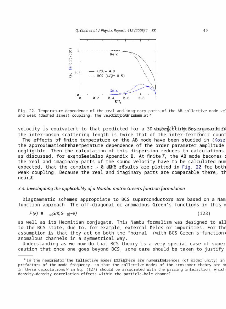
Q. Chen et al. / Physics Reports 412 (2005) 1 – 88 49
0.2 0.4 0.6 0.8T/ Tc
0
0.5
1
Re,
Im c
(T)/c
(0)
Re c
Im c
U/Uc = 0.9BCS (U/Uc = 0.5)
10
Fig. 22. Temperature dependence of the real and imaginary parts of the AB collective mode velocity for moderate (solid lines)and weak (dashed lines) coupling. The velocity vanishes atTc for both cases.
velocity is equivalent to that predicted for a 3D interacting Bose gasc = [4 naB/m2B]1/2. Here, as earlier,
the inter-boson scattering length is twice that of the inter-fermionic counterpart, at strong coupling. 6
The effects of finite temperature on the AB mode have been studied in (Kosztin et al., 2000), by makingthe approximation that the temperature dependence of the order parameter amplitude contribution isnegligible. Then the calculation of this dispersion reduces to calculations of the electromagnetic response,as discussed, for example in s. See also Appendix B. At finite T, the AB mode becomes damped andthe real and imaginary parts of the sound velocity have to be calculated numerically. Here one finds, asexpected, that the complex c → 0 as T → T c. The results are plotted in Fig. 22 for both moderate andweak coupling. Because the real and imaginary parts are comparable there, the mode is highly dampednear Tc.
3.3. Investigating the applicability of a Nambu matrix Green’s function formulation
Diagrammatic schemes appropriate to BCS superconductors are based on a Nambu matrix Green’sfunction approach. The off-diagonal or anomalous Green’s functions in this matrix are given by
F (K) ≡ scG(K)G 0(−K) (128)
as well as its Hermitian conjugate. This Nambu formalism was designed to allow study of perturbationsto the BCS state, due to, for example, external fields or impurities. For these perturbations the centralassumption is that they act on both the “normal” (with BCS Green’s function G(K) from Eq. (30)) andanomalous channels in a symmetrical way.
Understanding as we now do that BCS theory is a very special case of superconductivity, this raises thecaution that once one goes beyond BCS, some care should be taken to justify this Nambu approach. At
6 In the neutral case, for the full collective modes of Eq. (127), there are numerical differences (of order unity) in theprefactors of the mode frequency, so that the collective modes of the crossover theory are not strictly the same as in GP theory.In these calculations V in Eq. (127) should be associated with the pairing interaction, which enters in the context of fermionicdensity–density correlation effects within the particle–hole channel.

50 Q. Chen et al. / Physics Reports 412 (2005) 1 – 88
the very least the distinction between the order parameter sc and the excitation gap raises ambiguityabout applying a diagrammatic theory based on Nambu–Gor’kov Green’s functions.
More importantly, in treating the effects of the pseudogap self energy pg as we do here, it shouldbe clear that this self energy does not play a symmetric role in the anomalous and normal channels.It is viewed here as an entirely normal state effect. However this theory accommodates the equivalent(Kosztin et al., 2000) of the Nambu–Gor’kov “F”-function in general response functions such as in theMaki–Thompson diagrams of Appendix B through the asymmetric combinationGG0 which always arisesin pairs (for example, as the FF combinations of BCS theory). In this regard theGG0 formalism appearsto differ from all other T-matrix schemes which are designed to go below Tc, in that the Nambu schemeis not assumed at the start. Nevertheless, many features of this formalism seem to naturally arise in largepart because of Eq. (128), which demonstrates an intimate connection betweenGG0 and the conventionaldiagrams of BCS theory.
4. Other theoretical approaches to the crossover problem
4.1. T = 0 theories
We have noted in Section 1.7 that there are three main theoretical approaches to the crossover problembased on T-matrix theories. Their differences are associated with different forms for the pair susceptibility. The resulting calculations ofTc show similar variations. When two full Green’s functions are present in(as in the FLEX approach),Tc varies monotonically (Haussmann, 1993) with increasing attractive cou-
pling, approaching the ideal gas Bose–Einstein asymptote from below. When two bare Green’s functionsare present in , as in the work of Nozieres and Schmitt-Rink, and of Randeria and co-workers, then Tcovershoots (Sá de Melo et al., 1993; Nozières and Schmitt-Rink, 1985; Randeria, 1995) the BEC asymp-tote and ultimately approaches it from above. Finally when there is one bare and one dressed Green’sfunction, Tc first overshoots and then decreases to a minimum around = 0, eventually approachingthe asymptote from below (Maly et al., 1999b). This last appears to be a combination of the other twoapproaches. Overall the magnitudes are relatively similar and the quantitative differences are small. Thereis, finally, another body of work (Giovannini and Berthod, 2001) based on theGG0 scheme which shouldbe noted here. The approach by the Swiss group seeks to make contact with the phase fluctuation scenariofor high Tc superconductors and addresses STM and ARPES data.
Bigger differences appear when these T-matrix theories are extended below Tc. Detailed studies aremost extensive for the NSR approach. BelowTc one presumes that the T-matrix (or ) contains only bareGreen’s functions, but these functions are now taken to correspond to their Nambu matrix form, with theorder parameter sc appearing in the dispersion relation for excited fermions (Pieri et al., 2004; Randeria,1995). A motivation for generalizing the below- Tc T-matrix in this way is that one wants to connect tothe collective mode spectrum of the superconductor, so that the dispersion relation for pair excitations is
q ≈ cq. In this way the system would be more directly analogous to a true Bose system.Self energy effects are also incorporated below Tc but only in the number equation, either in the
approximate manner of NSR (Griffin and Ohashi, 2003; Randeria, 1995) or through use of the full Dysonresummation (Pieri et al., 2004) of the diagonal Nambu-matrix componentG( 0). For the latter scheme,Strinati’s group has addressed pseudogap effects in some detail with emphasis on the experimentallyobserved fermionic spectral function. Some concern can be raised that the fermionic excitations in the
Q. Chen et al. / Physics Reports 412 (2005) 1 – 88 51
gap equation do not incorporate this pseudogap, although these pairs are presumed to emerge out of anormal state which has a pseudogap. Indeed, this issue goes back to the original formulation of NSR,which includes self energy effects in the number equation, and not in the gap equation.
Tchernyshyov (Tchernyshyov, 1997) presented one of the first discussions belowTc for the FLEX-basedT-matrix scheme. He also addressed pseudogap effects and found a suppression of the fermion densityof states at low energy which allows for long-lived pair excitations inside this gap. At low momenta andfrequencies, their dispersion is that of a Bogoliubov-sound-like mode with a nonzero mass. Some ofthese ideas have been recently extended (Domanski and Ranninger, 2003) to apply to the boson–fermionmodel.
The work of Micnas and collaborators (Micnas et al., 1995) which is also based on the FLEX schemepredates the work of Tchernyshyov, although their initial focus was above Tc in two dimensional Hub-bard models. Here the fermionic spectral functions were studied in detail, using a numerically gen-erated solution of the T-matrix equations. A nice review of their large body of work on “real spacepairing” in the cuprates was presented based on a variety of different model Hamiltonians (Micnas andRobaszkiewicz, 1998).
An extensive body of work on the FLEX scheme has been contributed by Yamada and Yanatse (Yanaseet al., 2003) both above and belowTc. They point out important distinctions between their approach andthat of NSR. The effects of the broken symmetry are treated in a generalized Nambu formalism, muchas assumed by Pieri et al. (2004) and by Griffin and Ohashi (2003), but here the calculations involveself energy effects in both the number and gap equations. Their work has emphasized the effects of thepseudogap on magnetic properties, but they have discussed a wide variety of experiments in highTc andother exotic superconductors.
The nature of the ground states which result from these two alternatives ( ≈ GG and ≈ G0G0)has yet to be clearly established. It should be noted that, despite the extensive body of work based on theNSR or G0G0 scheme, no detailed picture has been presented in the literature of the nature of the groundstate which results when their calculations at Tc are extrapolated (Pieri et al., 2004) down to T = 0. Inlarge part, the differences between other work in the literature and that summarized in Sections 2.3 aredue to the whether (as in NSR-based papers) or not (as here) the superconducting order parameter scalone characterizes the fermionic dispersion below Tc.
One might well ask the question: because the underlying Hamiltonian [Eq. (11)] is associated withinter-fermionic, not inter-bosonic interactions, will this be reflected in the near-BEC limit of the crossoverproblem? The precise BEC limit is, of course, a noninteracting, or ideal Bose gas, but away from thislimit, fermionic degrees of freedom would seem to be relevant in ways that may not be accounted for bythe analogue treatment of the weakly interacting Bose gas. The most extensive study (albeit, above Tc)of this issue is due to Pieri and Strinati (2000). Their work, importantly, points out the inadequacies ofT-matrix schemes, particularly at strong coupling. While the ground state in their calculations is unknown,it is necessarily different from the conventional crossover state of Eq. (1). There is much intuition to begained by studying this simplest of all ground states, as outlined in this Review, but it will clearly be ofgreat value in future to consider states, in which, for example, there is less than full condensation.
Finally, we note that studies of non-s wave orbital pairing states in the context of the BCS–BECcrossover problem have rapidly proliferated in the literature. This is, in large part because of the observedd-wave pairing in the cuprates. Indeed, Leggett’s initial work (1980), addressed p-wave pairing in 3H e.Randeria (1995) also considered non-s wave pairing. Studies (Andrenacci et al., 1999; den Hertog, 1999)of this crossover for a d-wave lattice case are plentiful atT =0. Even earlier work was done (Chen et al.,
52 Q. Chen et al. / Physics Reports 412 (2005) 1 – 88
1999) on extensions of this ground state to include nonzero temperature. Moreover, a d-wave continuummodel has also been considered (Quintanilla et al., 2002). It is expected that in the near future cold atomexperiments will begin to address l = 0 pairing via appropriate choices of the Feshbach resonances(Ho and Zahariev, 2004).
4.2. Boson–Fermion models for high Tc superconductors
The notion that it might be appropriate to include bosonic degrees of freedom in highTc superconductorsgoes back to Lee and Friedberg who introduced (Friedberg and Lee, 1998a, b) the “boson–fermion” modelwithin three years of the discovery of cuprate superconductivity. The work of Lee and colleagues is basedon the Hamiltonian of Eq. (11) without the direct fermion–fermion interaction U. To our knowledge thisis the first study which argues for something akin to “real space pairing” in these materials. Interestingly,this work was motivated only by the observed short coherence length. Pseudogap effects, which makethis case much stronger, had not yet been properly characterized. The analogies with He 4 and a moreBEC-like picture of superconductivity were discussed, as well as the superfluid density, and energy gapstructure, albeit for s-wave pairing.
Subsequent work on this model Hamiltonian in the context of the high Tc copper oxides was pursuedby Ranninger and Micnas and their collaborators. Indeed, Ranninger and Robaszkiewicz (1985) were thefirst to write down the boson–fermion model, although initially, in an entirely different context, the bosonswere associated with phonons rather than electron pairs, and they were presumed to be localized. In thiscontext they addressed mean field theoretic solutions below Tc as well as more recently (Domanski andRanninger, 2003) an approach based on renormalization group techniques. The physical picture whichemerges leads to two gap structures below Tc, one associated with a pseudogap and another with thesuperconductivity. In this way it appears to be very different from approaches based on Eq. (1).
5. Physical implications: ultracold atom superfluidity
5.1. Homogeneous case
In this section we summarize the key characteristics of fermionic superfluidity in ultracold gases, inthe homogeneous situation, without introducing the trap potential. Our results are based on numericalsolution of the coupled Eqs. (69), (70) and (91). The upper left panel of Fig. 23 plots the fermionicchemical potential, the Feshbach boson condensate ratio and the inverse scattering length as a function of
0. Here we have chosen what we believe is the physically appropriate value for the Feshbach couplingg0 = −40EF/k 3
F for 40K, as determined from the experimentally measured scattering length data andresonance width.7 This parameter is roughly an order of magnitude larger for6Li. Here 0, the gaps and
are all in units of EF, and the plots, unless indicated otherwise, are at zero temperature.
7 We note that the precise values of g0 and U0 are not critical for either 6Li or 40K as long as they give roughly the right(large) resonance width B and background scatter lengthabg. In fact, these parameters usually change during experiment sincethe total particle number N (and hence EF and kF) decreases in the process of evaporative cooling. In order to compare withexperiment, one needs to compare at the correct value ofkFas.
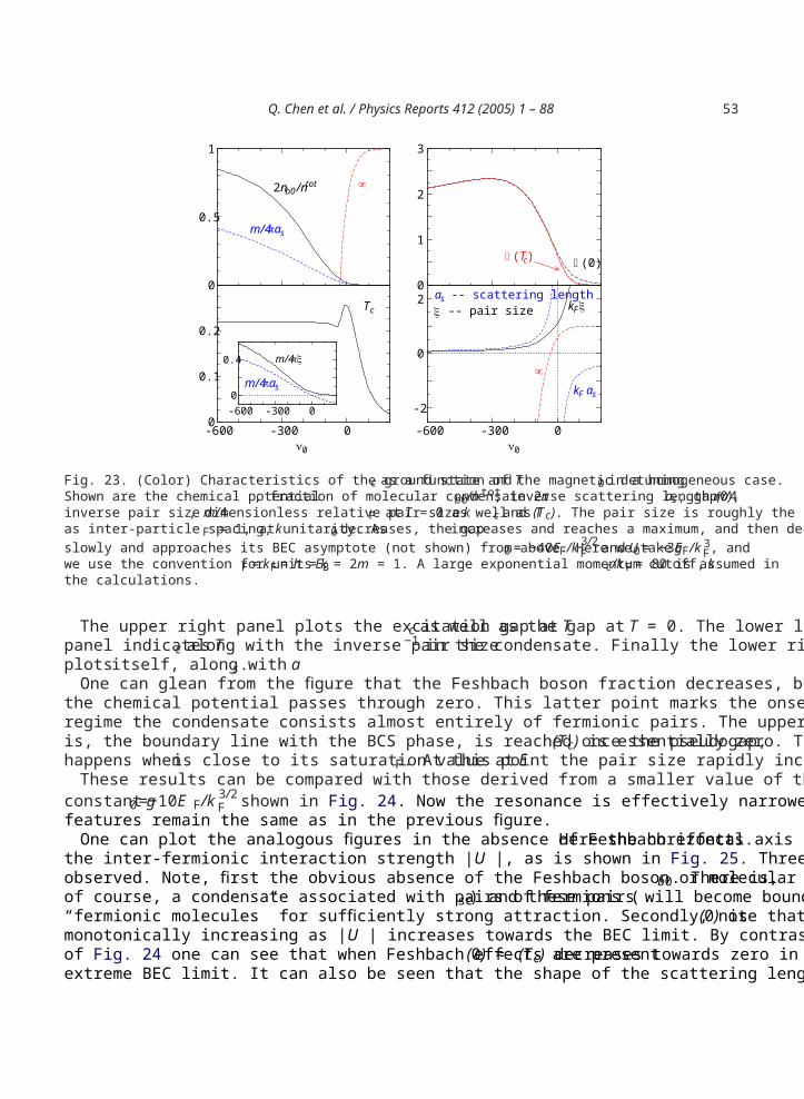
Q. Chen et al. / Physics Reports 412 (2005) 1 – 88 53
0
0.5
1
0
1
2
3
-600 -300 0
0
0.1
0.2
-600 -300 0ν0
-2
0
2
-600 -300 00
0.4 m/4πξ
∆(0)∆(Tc)
µ2nb0 /ntot
-- pair sizeas -- scattering length
m/4πas
Tc
kF as
kFξ
µ
m/4πas
ξ
ν0
Fig. 23. (Color) Characteristics of the ground state and Tc as a function of the magnetic detuning 0 in a homogeneous case.Shown are the chemical potential , fraction of molecular condensate 2nb0/n tot, inverse scattering length m/4 as, gap (0),inverse pair sizem/4 , dimensionless relative pair sizekF at T =0 as well as Tc and (Tc). The pair size is roughly the sameas inter-particle spacing,kF =1, at unitarity. As 0 decreases, the gap increases and reaches a maximum, and then decreasesslowly and approaches its BEC asymptote (not shown) from above. Here we takeg0 = −40EF/k 3/ 2
F and U0 = −3EF/k 3F , and
we use the convention for unitsEF = kF = h = kB =2m =1. A large exponential momentum cutoff,kc/kF =80 is assumed inthe calculations.
The upper right panel plots the excitation gap at Tc as well as the gap at T = 0. The lower left handpanel indicates Tc along with the inverse pair size −1 in the condensate. Finally the lower right panelplots itself, along with as.
One can glean from the figure that the Feshbach boson fraction decreases, becoming negligible whenthe chemical potential passes through zero. This latter point marks the onset of the PG regime, and in thisregime the condensate consists almost entirely of fermionic pairs. The upper limit of the PG regime, thatis, the boundary line with the BCS phase, is reached once the pseudogap, (Tc) is essentially zero. Thishappens when is close to its saturation value at EF. At this point the pair size rapidly increases.
These results can be compared with those derived from a smaller value of the Feshbach couplingconstant g0 =−10EF/k 3/2
F shown in Fig. 24. Now the resonance is effectively narrower. Other qualitativefeatures remain the same as in the previous figure.
One can plot the analogous figures in the absence of Feshbach effects. Here the horizontal axis isthe inter-fermionic interaction strength |U |, as is shown in Fig. 25. Three essential differences can beobserved. Note, first the obvious absence of the Feshbach boson or molecular condensate nb0. There is,of course, a condensate associated with pairs of fermions ( sc) and these pairs will become bound into“fermionic molecules” for sufficiently strong attraction. Secondly, note that the excitation gap (0) ismonotonically increasing as|U |increases towards the BEC limit. By contrast, from the upper right panelsof Fig. 24 one can see that when Feshbach effects are present (0) ≈ (Tc) decreases towards zero in theextreme BEC limit. It can also be seen that the shape of the scattering length curve vs. U is different from
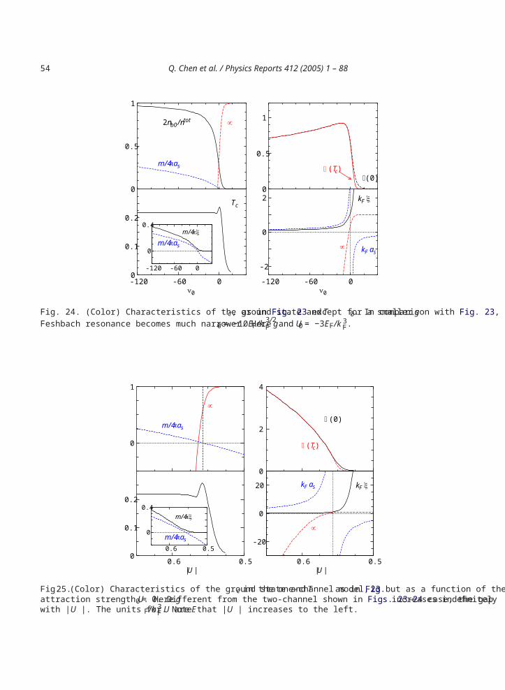
54 Q. Chen et al. / Physics Reports 412 (2005) 1 – 88
0
0.5
1
0
0.5
1
-120 -60 00
0.1
0.2
-120 -60 0
-2
0
2
-120 -60 0
0
0.4
∆(0)
m/4πξ
∆(Tc)
µ2nb0 /ntot
m/4πas
Tc
kF as
kF ξ
µ
m/4πas
ν0 ν0
Fig. 24. (Color) Characteristics of the ground state andTc, as in Fig. 23 except for a smallerg0. In comparison with Fig. 23, theFeshbach resonance becomes much narrower. Hereg0 = −10EF/k 3/ 2
F and U0 = −3EF/k 3F.
m/4πξ
∆(0)
∆(Tc)
µ
µm/4πas
kF as kF ξ
m/4πas
0
1
0
2
4
0.50.6|U |
0
0.1
0.2
0.50.6|U |
-20
0
20
0.50.6
0
0.4
Fig. 25. (Color) Characteristics of the ground state and Tc in the one-channel model, as in Fig. 23 but as a function of theattraction strength U. Here g0 = 0. Different from the two-channel shown in Figs. 23–24 case, the gap increases indefinitelywith |U |. The units for U are EF/k 3
F. Note that |U |increases to the left.
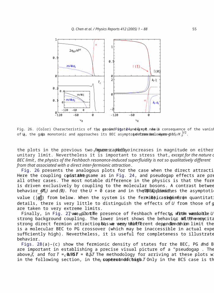
Q. Chen et al. / Physics Reports 412 (2005) 1 – 88 55
m/4πξ
∆(Tc)
µ
2nb0 /ntot
m/4πas
Tc
kF as
kF ξ
µ
m/4πas
ν0 ν0
0
0.5
1
0
0.5
1
-120 -60 00
0.1
0.2
-120 -60 0
-2
0
2
-120 -60 0
0
0.4
∆(0)
Fig. 26. (Color) Characteristics of the ground state andTc, as in Fig. 24, except nowU0 =0. As a consequence of the vanishingof U0, the gap is monotonic and approaches its BEC asymptote from below as 0 decreases. Here g0 = −10EF/K 3/2
F .
the plots in the previous two figures. Here as more rapidly increases in magnitude on either side of theunitary limit. Nevertheless it is important to stress that, except for the nature of the Bose condensate in theBEC limit, the physics of the Feshbach resonance-induced superfluidity is not so qualitatively differentfrom that associated with a direct inter-fermionic attraction.
Fig. 26 presents the analogous plots for the case when the direct attraction between fermions U vanishes.Here the coupling constant g0 is the same as in Fig. 24, and pseudogap effects are present here just as inall other cases. The most notable difference in the physics is that the formation of the Cooper condensateis driven exclusively by coupling to the molecular bosons. A contrast between the two figures is in thebehavior of (Tc) and (0). For the U = 0 case and in the BEC limit, (0) approaches the asymptoticvalue (|g| n0
b) from below. When the system is the fermionic regime ( >0), aside from quantitativedetails, there is very little to distinguish the effects of U from those of g, except when these parametersare taken to very extreme limits.
Finally, in Fig. 27 we plotTc vs. 0 in the presence of Feshbach effects with variableU0, from weak tostrong background coupling. The lower inset shows the behavior of the excitation gap at Tc. With verystrong direct fermion attraction U, we see thatTc has a very different dependence on 0. In this limit thereis a molecular BEC to PG crossover (which may be inaccessible in actual experiments, since U is notsufficiently high). Nevertheless, it is useful for completeness to illustrate the entire range of theoreticalbehavior.
Figs. 28(a)–(c) show the fermionic density of states for the BEC, PG and BCS limits. These figuresare important in establishing a precise visual picture of a “pseudogap”. The temperatures shown are justabove Tc, and forT =0.75Tc and T =0.5Tc. The methodology for arriving at these plots will be discussedin the following section, in the context of high Tc superconductors. Only in the BCS case is there a clear
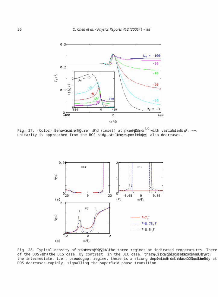
56 Q. Chen et al. / Physics Reports 412 (2005) 1 – 88
-400 0 400
ν0 /EF
0
0.1
0.2
0.3
T c /E
FU0 = -100
-80
-40
-20
-10
U0 = -3-800 0 4000
1
2
∆ (T c
)/EF
U0 = -3
-10
-20
-40 -100-80
Fig. 27. (Color) Behavior of Tc (main figure) and (Tc) (inset) at fixed g0 = −40EF/k 3/ 2F with variable U0. As U0 → −∞ ,
unitarity is approached from the BCS side at large positive 0. At the same time, ∝ |g|also decreases.
-20 0 200
0.01
T=Tc+
T=0.75 Tc
T=0.5 Tc
-2 0ω/EF
0
0.3
N(ω
)
-0.05 0 0.050
1
2BEC
PG
BCS
2
ω/EF
N(ω
)
(a) (c)
(b)
Fig. 28. Typical density of states (DOS)N( ) vs energy in the three regimes at indicated temperatures. There is no depletionof the DOS at Tc in the BCS case. By contrast, in the BEC case, there is a large gap in DOS atTc, roughly determined by| |. Inthe intermediate, i.e., pseudogap, regime, there is a strong depletion of the DOS already at Tc. Once T decreases below Tc, theDOS decreases rapidly, signalling the superfluid phase transition.
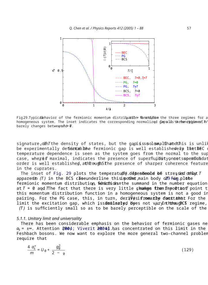
Q. Chen et al. / Physics Reports 412 (2005) 1 – 88 57
0 2k/kF
0
0.5
1
n k
BEC, T=0,T=Tc
PG, T=0PG, T=Tc
BCS, T=0BCS, T=Tc
0T/Tc
0
1
∆ (T)
/∆(0
)
BECPGBCS
1 3
1
Fig. 29. Typical behavior of the fermionic momentum distribution function nk at T = 0 and Tc in the three regimes for ahomogeneous system. The inset indicates the corresponding normalized gaps as a function of T /Tc. In all three regimes, nkbarely changes between T = Tc and 0.
signature of Tc in the density of states, but the gap is so small and Tc is so low, that this is unlikely tobe experimentally detectable. Since the fermionic gap is well established in the BEC case, very littletemperature dependence is seen as the system goes from the normal to the superfluid states. Only the PGcase, where Tc is maximal, indicates the presence of superfluidity, not so much at Tc but once superfluidorder is well established at T =0.5Tc, through the presence of sharper coherence features, much as seenin the cuprates.
The inset of Fig. 29 plots the temperature dependence of (T ). It should be stressed that Tc is onlyapparent in (T ) in the BCS case. To underline this point, in the main body of Fig. 29 we plot thefermionic momentum distribution function nk, which is the summand in the number equation, Eq. (70),at T = 0 and Tc. The fact that there is very little change from T = 0 to Tc makes the important point thatthis momentum distribution function in a homogeneous system is not a good indicator of phase coherentpairing. For the PG case, this, in turn, derives from the fact that (T )is nearly constant. For the BEClimit the excitation gap, which is dominated by , similarly, does not vary throughTc. In the BCS regime,(T )is sufficiently small so as to be barely perceptible on the scale of the figure.
5.1.1. Unitary limit and universalityThere has been considerable emphasis on the behavior of fermionic gases near the unitary limit where
as = ±∞. Attention (Ho, 2004; Viverit et al., 2004) has concentrated on this limit in the absence ofFeshbach bosons. We now want to explore the more general two-channel problem here. At unitarity werequire that
4 a∗s
m= U0 + g2
02 − 0
(129)
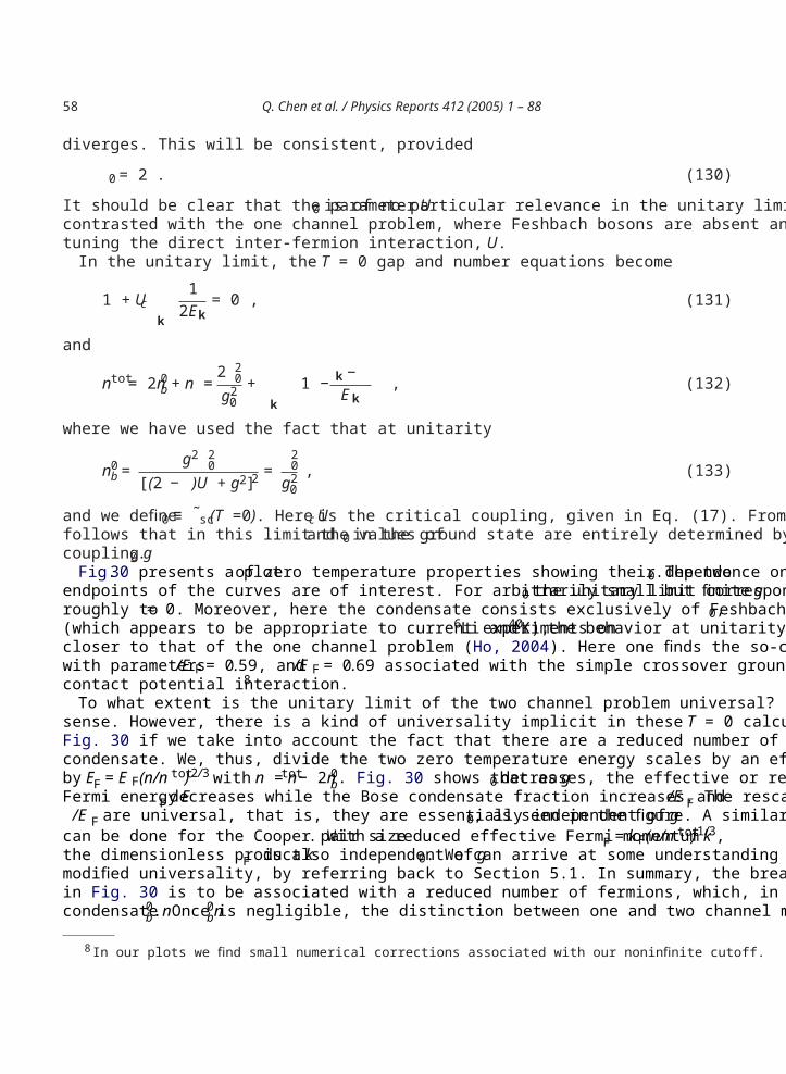
58 Q. Chen et al. / Physics Reports 412 (2005) 1 – 88
diverges. This will be consistent, provided
0 = 2 . (130)
It should be clear that the parameter U0 is of no particular relevance in the unitary limit. This is to becontrasted with the one channel problem, where Feshbach bosons are absent and unitarity is achieved bytuning the direct inter-fermion interaction, U.
In the unitary limit, the T = 0 gap and number equations become
1 + Uck
12Ek
= 0 , (131)
and
ntot = 2n0b + n =2 2
0g2
0+
k1 − k −
Ek, (132)
where we have used the fact that at unitarity
n0b = g2 2
0[(2 − )U + g2]2 =
20
g20
, (133)
and we define 0 ≡ ˜sc(T =0). Here Uc is the critical coupling, given in Eq. (17). From these equations itfollows that in this limit the values of and 0 in the ground state are entirely determined by the Feshbachcoupling g0.
Fig. 30 presents a plot of zero temperature properties showing their dependence on g0. The twoendpoints of the curves are of interest. For arbitrarily small but finite g0 the unitary limit correspondsroughly to ≈ 0. Moreover, here the condensate consists exclusively of Feshbach bosons. At large g0,(which appears to be appropriate to current experiments on 6Li and 40K), the behavior at unitarity iscloser to that of the one channel problem (Ho, 2004). Here one finds the so-called universal behaviorwith parameters /E F = 0.59, and /E F =0.69 associated with the simple crossover ground state and acontact potential interaction.8
To what extent is the unitary limit of the two channel problem universal? It clearly is not in an absolutesense. However, there is a kind of universality implicit in these T = 0 calculations, as can be seen fromFig. 30 if we take into account the fact that there are a reduced number of fermions, as a result of the Bosecondensate. We, thus, divide the two zero temperature energy scales by an effective Fermi energy definedby EF = EF(n/ntot)2/3 with n = ntot − 2n0
b. Fig. 30 shows that as g0 decreases, the effective or rescaledFermi energyEF decreases while the Bose condensate fraction increases. The rescaled quantities/E F and/E F are universal, that is, they are essentially independent ofg0, as seen in the figure. A similar scaling
can be done for the Cooper pair size . With a reduced effective Fermi momentum kF = kF(n/ntot)1/3,the dimensionless product kF is also independent of g0. We can arrive at some understanding of thismodified universality, by referring back to Section 5.1. In summary, the breakdown of universality seenin Fig. 30 is to be associated with a reduced number of fermions, which, in turn derives from the Bosecondensate n0
b. Once n0b is negligible, the distinction between one and two channel models disappears.
8 In our plots we find small numerical corrections associated with our noninfinite cutoff.
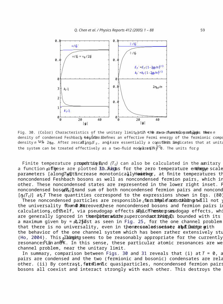
Q. Chen et al. / Physics Reports 412 (2005) 1 – 88 59
0
0.4
0.8
0
0.4
0.8
0 20 40 0 20 40|g0 | |g0 |
0
1
2
3
0
0.4
0.8
µ/EF = ν0 /2EF
∆/EF
∆/EF′
EF′ =EF(1-2nb0 /n)2/3
2nb0 /n
kF′ =kF(1-2nb0 /n)1/3
kF ξ
k′F ξ
µ/EF′
Fig. 30. (Color) Characteristics of the unitary limit at T = 0 as a function of |g0| in the two-channel problem. Here nb0 is thedensity of condensed Feshbach bosons. EF = kF
2/2mdefines an effective Fermi energy of the fermionic component with adensity n = ntot − 2nb0. After rescaling, /E F , /E F, and kF are essentially a constant in g0. This indicates that at unitarity,the system can be treated effectively as a two-fluid model atT = 0. The units for g0 are EF/k 3/ 2
F .
Finite temperature properties, such as Tc and (Tc) can also be calculated in the unitary limit, asa function of g0. These are plotted in Fig. 31. Just as for the zero temperature energy scales, theseparameters [along with (Tc)] increase monotonically with g0. However, at finite temperatures there arenoncondensed Feshbach bosons as well as noncondensed fermion pairs, which interact strongly with eachother. These noncondensed states are represented in the lower right inset. Plotted there is the fraction ofnoncondensed bosons [nb(Tc)] and sum of both noncondensed fermion pairs and noncondensed bosons[np(Tc)] at Tc. These quantities correspond to the expressions shown in Eqs. (80) and (92), respectively.
These noncondensed particles are responsible for the fact that at Tc a simple rescaling will not yieldthe universality found at T = 0. Moreover, these noncondensed bosons and fermion pairs influencecalculations of Tc, itself, via pseudogap effects which enter as (Tc). These pseudogap effects, whichare generally ignored in the literature, compete with superconductivity, so that Tc is bounded with itsa maximum given by ≈ 0.25TF, just as seen in Fig. 25, for the one channel problem. Despite the factthat there is no universality, even in the rescaled sense, at Tc one can associate the large g0 limits withthe behavior of the one channel system which has been rather extensively studied in the unitary limit(Ho, 2004). This large g0 limit seems to be reasonably appropriate for the currently studied Feshbachresonances in 6Li and 40K. In this sense, these particular atomic resonances are well treated by a onechannel problem, near the unitary limit.
In summary, comparison between Figs. 30 and 31 reveals that (i) at T = 0, all Feshbach bosons andpairs are condensed and the two (fermionic and bosonic) condensates are relatively independent of eachother. (ii) By contrast, at T = Tc, fermionic quasiparticles, noncondensed fermion pairs and Feshbachbosons all coexist and interact strongly with each other. This destroys the simple scaling found atT =0.
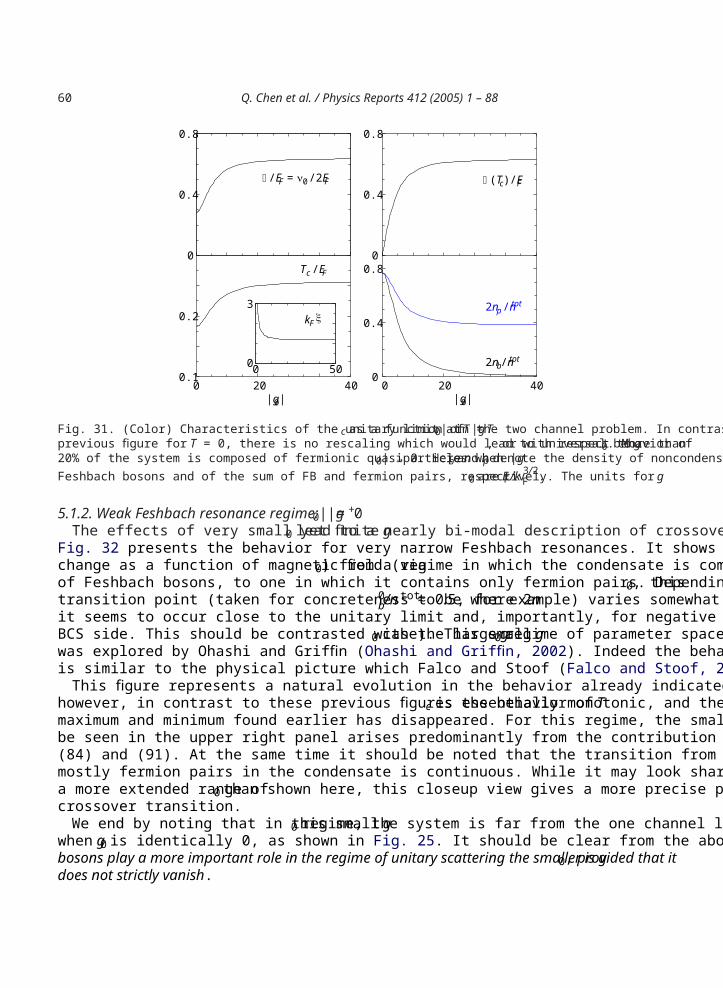
60 Q. Chen et al. / Physics Reports 412 (2005) 1 – 88
0
0.4
0.8
0
0.4
0.8
0.1
0.2
0
0.4
0.8
00
3
µ/EF = ν0 /2EF ∆(Tc)/EF
2nb/ntot
kF
Tc /EF
2np /ntot
0 20 40 0 20 40|g0 | |g0 |
50
ξ
Fig. 31. (Color) Characteristics of the unitary limit atT = Tc as a function of |g0| in the two channel problem. In contrast to theprevious figure forT =0, there is no rescaling which would lead to universal behavior of , or with respect tog0. More than20% of the system is composed of fermionic quasiparticles when|g0| → 0. Here nb and np denote the density of noncondensedFeshbach bosons and of the sum of FB and fermion pairs, respectively. The units forg0 are EF/k 3/2
F .
5.1.2. Weak Feshbach resonance regime:|g0| =0+The effects of very small yet finite g0 lead to a nearly bi-modal description of crossover phenomena.
Fig. 32 presents the behavior for very narrow Feshbach resonances. It shows that there is a rather abruptchange as a function of magnetic field (via 0) from a regime in which the condensate is composed onlyof Feshbach bosons, to one in which it contains only fermion pairs. Depending on the size of g0, thistransition point (taken for concreteness to be where 2 n0
b/n tot ≈ 0.5, for example) varies somewhat, butit seems to occur close to the unitary limit and, importantly, for negative scattering lengths i.e., on theBCS side. This should be contrasted with the large g0 case). This small g0 regime of parameter spacewas explored by Ohashi and Griffin (Ohashi and Griffin, 2002). Indeed the behavior shown in the figureis similar to the physical picture which Falco and Stoof (Falco and Stoof, 2004) presented.
This figure represents a natural evolution in the behavior already indicated by Figs. 23 and 24. Here,however, in contrast to these previous figures the behavior of Tc is essentially monotonic, and the weakmaximum and minimum found earlier has disappeared. For this regime, the small pseudogap which canbe seen in the upper right panel arises predominantly from the contribution of Feshbach bosons via Eqs.(84) and (91). At the same time it should be noted that the transition from mostly molecular bosons tomostly fermion pairs in the condensate is continuous. While it may look sharp particularly for a plot witha more extended range of 0 than shown here, this closeup view gives a more precise picture of a smoothcrossover transition.
We end by noting that in this small g0 regime, the system is far from the one channel limit obtainedwhen g0 is identically 0, as shown in Fig. 25. It should be clear from the above discussion that Feshbachbosons play a more important role in the regime of unitary scattering the smaller is g0, provided that itdoes not strictly vanish.
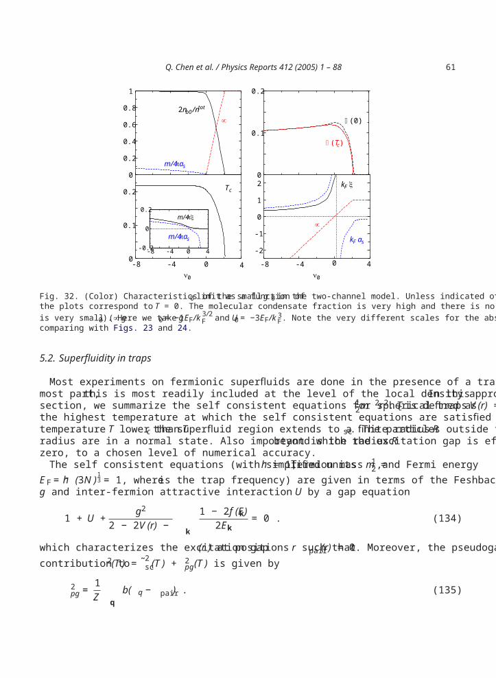
Q. Chen et al. / Physics Reports 412 (2005) 1 – 88 61
0
0.2
0.4
0.6
0.8
1
0
0.1
0.2
-8 -4 00
0.1
0.2
-8 -4
-2
-1
0
1
2
-8 -4 0-0.2
0
0.2
Tc
m/4πξ
∆(0)
∆(Tc)
µ
µ
m/4πas kF as
kF ξ
m/4πas
4 0 4ν0 ν0
2nb0 /ntot
4
Fig. 32. (Color) Characteristics of the small g0 limit as a function of 0 in the two-channel model. Unless indicated otherwisethe plots correspond to T = 0. The molecular condensate fraction is very high and there is no maximum at unitarity. The gapis very small (∝ g0). Here we take g0 = −1EF/k 3/2
F and U0 = −3EF/k 3F. Note the very different scales for the abscissa when
comparing with Figs. 23 and 24.
5.2. Superfluidity in traps
Most experiments on fermionic superfluids are done in the presence of a trap potential V (r). For themost part, this is most readily included at the level of the local density approximation (LDA). In thissection, we summarize the self consistent equations for spherical traps V (r) =1
2m 2r2. Tc is defined asthe highest temperature at which the self consistent equations are satisfied precisely at the center. At atemperature T lower than Tc the superfluid region extends to a finite radiusRsc. The particles outside thisradius are in a normal state. Also important is the radiusR beyond which the excitation gap is effectivelyzero, to a chosen level of numerical accuracy.
The self consistent equations (with simplified units h =1, fermion mass m =12 , and Fermi energy
EF = h (3N) 13 =1, where is the trap frequency) are given in terms of the Feshbach coupling constant
g and inter-fermion attractive interaction U by a gap equation
1 + U + g2
2 − 2V (r) −k
1 − 2f (Ek)2Ek
= 0 . (134)
which characterizes the excitation gap (r )at positions r such that pair(r) =0. Moreover, the pseudogapcontribution to 2(T ) =˜2
sc(T ) + 2pg(T )is given by
2pg = 1
Z qb( q − pair) . (135)
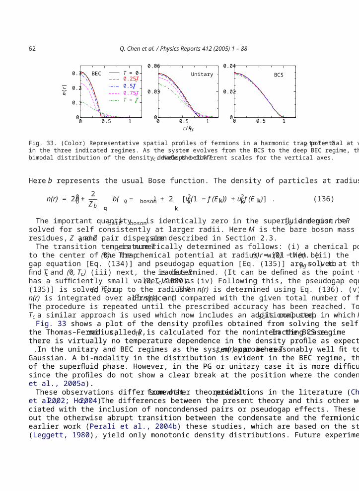
62 Q. Chen et al. / Physics Reports 412 (2005) 1 – 88
0 0.5 1 0 0.5 1 0 0.5 10
0.1
0.2
0.3
n(r)
T = 00.25Tc0.5Tc0.75TcT = Tc
r/RTF
0
0.03
0.06
0
0.02
0.04BEC Unitary BCS
Fig. 33. (Color) Representative spatial profiles of fermions in a harmonic trap potential at various temperatures fromTc to T =0in the three indicated regimes. As the system evolves from the BCS to the deep BEC regime, the fermion cloud shrinks, and abimodal distribution of the density develops belowTc. Note the different scales for the vertical axes.
Here b represents the usual Bose function. The density of particles at radius r:
n(r) =2n0b + 2
Zb qb( q − boson) +2
k[v2
k(1 − f (Ek)) + u2kf (Ek)] . (136)
The important quantity pair = boson is identically zero in the superfluid region r < Rsc, and must besolved for self consistently at larger radii. Here M is the bare boson mass equal to 2 m, and the variousresidues, Z and Zb and pair dispersion q are described in Section 2.3.
The transition temperature Tc is numerically determined as follows: (i) a chemical potential is assignedto the center of the trap (0). The chemical potential at radius r will then be (r) = (0) − V (r). (ii) thegap equation [Eq. (134)] and pseudogap equation [Eq. (135)] are solved at the center (setting pg= ) tofind Tc and (0, Tc) (iii) next, the radius R is determined. (It can be defined as the point where the gaphas a sufficiently small value, such as (0, Tc)/1000). (iv) Following this, the pseudogap equation [Eq.(135)] is solved for (r, Tc) up to the radius R . Then n(r) is determined using Eq. (136). (v) Finally,n(r) is integrated over all space ( d3rn(r)) and compared with the given total number of fermions N.The procedure is repeated until the prescribed accuracy has been reached. To extend this algorithm belowTc a similar approach is used which now includes an additional step in which Rsc is computed.
Fig. 33 shows a plot of the density profiles obtained from solving the self consistent equations. Herethe Thomas–Fermi radius, called RTF, is calculated for the noninteracting case. In the BCS regimethere is virtually no temperature dependence in the density profile as expected from the small values for
. In the unitary and BEC regimes as the system approaches Tc, n(r) can be reasonably well fit to aGaussian. A bi-modality in the distribution is evident in the BEC regime, thus providing a clear signatureof the superfluid phase. However, in the PG or unitary case it is more difficult to establish superfluidity,since the profiles do not show a clear break at the position where the condensate first appears (Stajicet al., 2005a).
These observations differ somewhat from other theoretical predictions in the literature (Chiofaloet al., 2002; Ho, 2004). The differences between the present theory and this other work can be asso-ciated with the inclusion of noncondensed pairs or pseudogap effects. These noncondensed pairs smoothout the otherwise abrupt transition between the condensate and the fermionic excitations. In contrast toearlier work (Perali et al., 2004b) these studies, which are based on the standard crossover ground state(Leggett, 1980), yield only monotonic density distributions. Future experiments will be needed to look
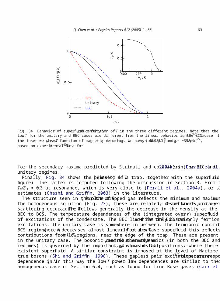
Q. Chen et al. / Physics Reports 412 (2005) 1 – 88 63
0 0.5 1
T/Tc
0
0.5
1
NS(
T)/N
S(0)
BCSUnitary
BEC
-200 0-400ν0 /EF
0
0.2
0.4
T c/E
F
Fig. 34. Behavior of superfluid densityNs as a function of T in the three different regimes. Note that the negative curvatures atlow T for the unitary and BEC cases are different from the linear behavior in the BCS case. In the BEC limit,N −Ns ∝ T3/ 2. Inthe inset we show Tc as a function of magnetic detuning 0 in a trap. We have takenU0 = −0.9EF/k 3
F and g0 = −35EF/k 3/2F ,
based on experimental data for 40K.
for the secondary maxima predicted by Strinati and co-workers (Perali et al., 2004a) in the BEC andunitary regimes.
Finally, Fig. 34 shows the behavior of Tc (inset) in a trap, together with the superfluid density (mainfigure). The latter is computed following the discussion in Section 3. From the inset one can read off thatTc/E F ≈ 0.3 at resonance, which is very close to (Perali et al., 2004a), or slightly smaller than otherestimates (Ohashi and Griffin, 2003) in the literature.
The structure seen in the plot of Tc for the trapped gas reflects the minimum and maximum found forthe homogeneous solution (Fig. 23); these are related, respectively, to where ≈ 0 and where unitaryscattering occurs. The Tc curve follows generally the decrease in the density at the center of the trap fromBEC to BCS. The temperature dependences of the (integrated over r) superfluid density reflect the natureof excitations of the condensate. The BEC limit has only bosonic, while the BCS has only fermionicexcitations. The unitary case is somewhere in between. The fermionic contributions are apparent in theBCS regime, where Ns decreases almost linearly at low T. For an s-wave superfluid this reflects thecontributions from low (r )⩽T regions, near the edge of the trap. These are present to a lesser degreein the unitary case. The bosonic contribution toNs and to thermodynamics (in both the BEC and unitaryregimes) is governed by the important constraint that pair(r )vanishes at positions r where there is a co-existent superfluid. A similar constraint is imposed at the level of Hartree–Fock–Bogoliubov theory fortrue bosons (Shi and Griffin, 1998). These gapless pair excitations are responsible for aT 3/2 temperaturedependence in Ns. In this way the low T power law dependences are similar to their analogues in thehomogeneous case of Section 6.4, much as found for true Bose gases (Carr et al., 2004) in a trap.
64 Q. Chen et al. / Physics Reports 412 (2005) 1 – 88
As for the BEC regime there is an interesting observation to make about the contribution to the densityprofile associated with the condensate. Experimentalists generally assume a Gaussian form throughoutthe trap for the noncondensed pairs. In this way they estimate the condensate fraction. Here we find(Stajic et al., 2005a) that this Gaussian form is not correct in the superfluid region of the trap, and thatthis Gaussian approximation will underestimate (by≈ a factor of 1.5) the condensate fraction in the BECregime.
5.3. Comparison between theory and experiment: cold atoms
As time progresses it will be important to assess the assumed ground state wavefunction (Leggett, 1980)and its two channel variant (Milstein et al., 2002; Ohashi and Griffin, 2002; Stajic et al., 2005b) in moredetail. A first generation set of measurements and theories have indicated an initial level of success inaddressing four experiments: RF pairing gap spectroscopy and collective mode measurements, as well asmore recently, the particle density profiles (Stajic et al., 2005a) and thermodynamics (Kinast et al., 2005)of Fermi gases in the unitary regime. The first of these experiments (Chin et al., 2004) seem to providesome support for the fact that the Bogoliubov excitations with dispersion, Ek ≡ ( k − )2 + 2(T )have a “gap parameter”, (T )which is in general different from the superconducting order parameter,as a consequence of noncondensed pairs at and aboveTc. Torma and colleagues (Kinnunen et al., 2004b)have used the formalism outlined in Section 2.2, to address RF spectroscopy. Subsequently (Kinnunenet al., 2004a) they have combined this analysis with an approximate LDA treatment of the trap to makecontact with RF experiments (Chin et al., 2004). Important to their work is the fact that the edges of atrap have a free atom character, where there is a vanishing (r ).
Additional support for the wavefunction comes from the collective mode behavior nearT =0. The modefrequencies can be connected to an equation of state (Stringari, 2004). Numerical studies (Heiselberg,2004b; Hu et al., 2004) of this equation for the standard crossover ground state demonstrate a good fitto the measured breathing mode frequencies (Bartenstein et al., 2004a; Kinast et al., 2004). Importantly,in the near-BEC limit the frequencies decrease with increasing magnetic field; this is opposite to thebehavior predicted for true bosons (Stringari, 2004), and appears to reenforce the notion that for themagnetic fields studied thus far, the “BEC” regime should be associated with composite rather than realbosons.
At T =0, calculations of the collective mode frequencies are based on an equation of state. Moreover,the zero temperature equation of state associated with the mean field ground state can be computedanalytically in the near-BEC limit
= − 12ma2
s+ asn
m− 3( na3
s)2
4ma2s
+ O(n3) ,
where the first two terms on the right hand side were previously discussed following Eq. (55). Importantly,the third (negative) term is responsible for the observed agreement between theory and collective modeexperiments, in the near-BEC regime.
A serious shortcoming of the wavefunction ansatz has been emphasized in the literature. This is associ-ated with the ratio of the inter-boson to the fermionic scattering length near the unitary regime, but on theBEC side of the Feshbach resonance. Experimentally the numbers are considerably smaller (Bartensteinet al., 2004b; Zwierlein et al., 2004) (0 .6) than the factor of 2 predicted for the one channel model dis-cussed below Eq. (55). They are consistent, however, with more exact few body calculations (Petrov et
Q. Chen et al. / Physics Reports 412 (2005) 1 – 88 65
al., 2004). These few body calculations presumably apply to a regime of magnetic fields where kFas isaround 0.3–0.4 or smaller. This seems to be close to the boundary for the “quasi-BEC” regime which canbe accessed experimentally (Bartenstein et al., 2004b) in 6Li.
It is interesting to repeat the T = 0 many body calculations now with the inclusion of FB, since (for∼ 40 K) these two channel effects begin to be important atkFas smaller than around 0.2–0.25. Here, onesees (Stajic et al., 2005b), that the factor of 2 found in the one channel calculations is no longer applicable,and the values of the ratio (of bosonic to fermionic scattering lengths) are considerably smaller, and, thus,tending in the direction which is more in line with experiment. This reflects the decrease in the numberof fermionic states which mediate the interaction between molecular bosons.
In this way the mean field theory presented here looks promising. Nevertheless, uncertainties remain.Current theoretical work (Kinnunen et al., 2004a) on the RF experiments is limited to the intermediatecoupling phase, while experiments are also available for the near-BEC and near-BCS regimes, and shouldbe addressed theoretically. In addition, the predictions of alternative approaches (Perali et al., 2004b)which posit a different ground state will need to be compared with these RF data. The collective modecalculations (Heiselberg, 2004b; Hu et al., 2004) which have been performed have not yet considered theeffects of Feshbach bosons, which may change the behavior in the deeper BEC regime.
It is, finally, quite possible that incomplete T = 0 condensation will become evident in future ex-periments. If so, an alternative wavefunction will have to be contemplated. Indeed, it has been argued(Holland et al., 2004) that the failure of the one channel model to match the calculations of Petrov andco-workers (Petrov et al., 2004) is evidence that there are serious weaknesses. At an experimental level,new pairing gap spectroscopies appear to be emerging at a fairly rapid pace (Bruun and Baym, 2004;Greiner et al., 2005) which will further test these and subsequent theories.
6. Physical implications: high Tc superconductivity
We begin with an important caveat that many of the experiments outlined in this section can alternativelybe addressed from a Mott physics point of view (Lee et al., 2004). Here we summarize the interpretationof these experiments within BCS–BEC crossover theory with the hope that this discussion will be ofvalue to the cold atom community, and that ultimately, it will help to establish precisely how relevant isthe BCS–BEC crossover scenario for understanding high temperature superconductivity.
6.1. Phase diagram and superconductor–insulator transition: boson localization effects
The high Tc superconductors are different from the ultracold fermionic superfluids in one key respect;they are d-wave superconductors and their electronic dispersion is associated with a quasi-two dimensionaltight binding lattice. In many ways this is not a profound difference from the perspective of BCS–BECcrossover. Fig. 35 shows a plot of the two important temperatures Tc and T∗as a function of increasingattractive coupling. On the left is BCS and the right is PG. The BEC regime is not apparent. This isbecause Tc disappears before it can be accessed. At the point where Tc vanishes, /E F ≈ 0.8.
A competition between increasing T∗ and Tc is also apparent in Fig. 35. This is a consequence ofpseudogap effects. There are fewer low energy fermions around to pair, as T∗increases. It is interestingto compare Fig. 35 with the experimental phase diagram plotted as a function of x in Fig. 7. If one invertsthe horizontal axis (and ignores the AFM region, which is not addressed here) the two are very similar. To
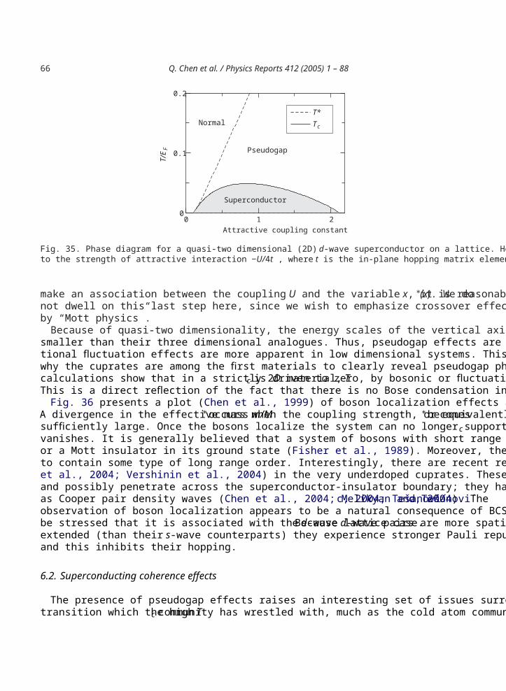
66 Q. Chen et al. / Physics Reports 412 (2005) 1 – 88
0 2Attractive coupling constant
0
0.1
0.2
T/E F Pseudogap
Superconductor
NormalT*Tc
1
Fig. 35. Phase diagram for a quasi-two dimensional (2D) d-wave superconductor on a lattice. Here the horizontal axis correspondsto the strength of attractive interaction−U/4t, where t is the in-plane hopping matrix element.
make an association between the coupling U and the variable x, it is reasonable to simply fitT∗(x). We donot dwell on this last step here, since we wish to emphasize crossover effects which are not complicatedby “Mott physics”.
Because of quasi-two dimensionality, the energy scales of the vertical axis in Fig. 35 are considerablysmaller than their three dimensional analogues. Thus, pseudogap effects are intensified, just as conven-tional fluctuation effects are more apparent in low dimensional systems. This may be one of the reasonswhy the cuprates are among the first materials to clearly reveal pseudogap physics. Moreover, the presentcalculations show that in a strictly 2 D material, Tc is driven to zero, by bosonic or fluctuation effects.This is a direct reflection of the fact that there is no Bose condensation in 2D.
Fig. 36 presents a plot (Chen et al., 1999) of boson localization effects associated with d-wave pairing.A divergence in the effective massm/M∗occurs when the coupling strength, or equivalentlyT∗becomessufficiently large. Once the bosons localize the system can no longer support superconductivity and Tcvanishes. It is generally believed that a system of bosons with short range repulsion is either a superfluidor a Mott insulator in its ground state (Fisher et al., 1989). Moreover, the insulating phase is presumedto contain some type of long range order. Interestingly, there are recent reports of ordered phases (Fuet al., 2004; Vershinin et al., 2004) in the very underdoped cuprates. These appear on the insulating sideand possibly penetrate across the superconductor-insulator boundary; they have been interpreted by someas Cooper pair density waves (Chen et al., 2004; Melikyan and Tešanovic, 2004; Tešanovic, 2004). Theobservation of boson localization appears to be a natural consequence of BCS–BEC theory; it shouldbe stressed that it is associated with the d-wave lattice case. Because d-wave pairs are more spatiallyextended (than their s-wave counterparts) they experience stronger Pauli repulsion (Chen et al., 1999)and this inhibits their hopping.
6.2. Superconducting coherence effects
The presence of pseudogap effects raises an interesting set of issues surrounding the signatures of thetransition which the high Tc community has wrestled with, much as the cold atom community is doing
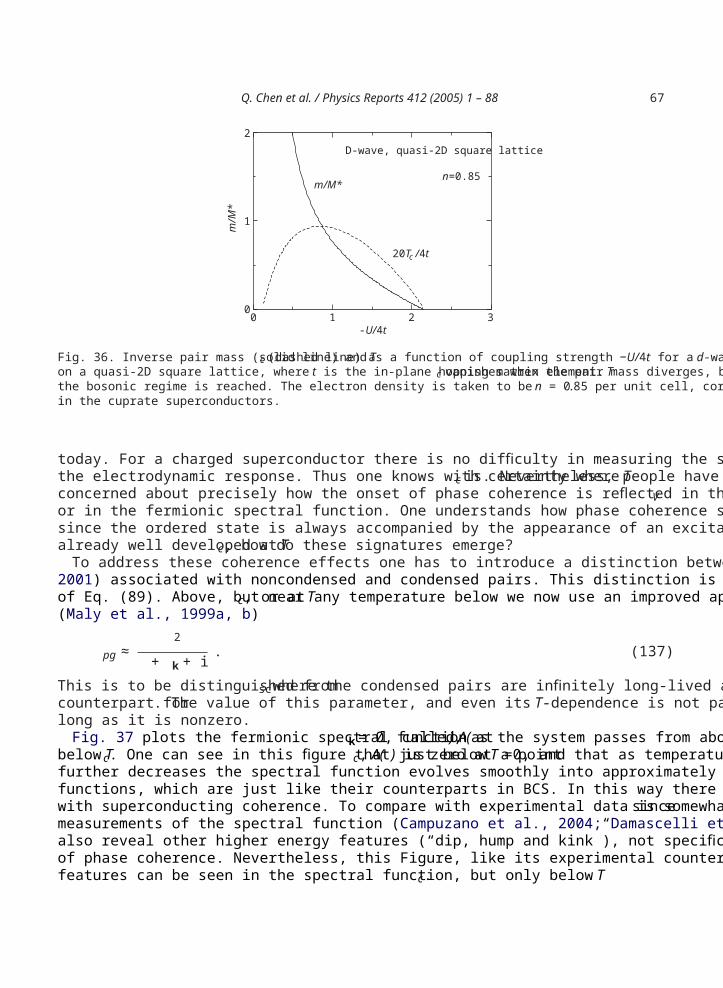
Q. Chen et al. / Physics Reports 412 (2005) 1 – 88 67
0 2-U/4t
0
1
2
m/M
*
20Tc /4t
m/M*
D-wave, quasi-2D square lattice
n=0.85
31
Fig. 36. Inverse pair mass (solid line) andTc (dashed line) as a function of coupling strength−U/4t for a d-wave superconductoron a quasi-2D square lattice, where t is the in-plane hopping matrix element. Tc vanishes when the pair mass diverges, beforethe bosonic regime is reached. The electron density is taken to ben =0.85 per unit cell, corresponding to optimal hole dopingin the cuprate superconductors.
today. For a charged superconductor there is no difficulty in measuring the superfluid density, throughthe electrodynamic response. Thus one knows with certainty whereTc is. Nevertheless, people have beenconcerned about precisely how the onset of phase coherence is reflected in thermodynamics, such asCVor in the fermionic spectral function. One understands how phase coherence shows up in BCS theory,since the ordered state is always accompanied by the appearance of an excitation gap. When a gap isalready well developed at Tc, how do these signatures emerge?
To address these coherence effects one has to introduce a distinction between the self energy (Chen et al.,2001) associated with noncondensed and condensed pairs. This distinction is blurred by the approximationof Eq. (89). Above, but near Tc, or at any temperature below we now use an improved approximation(Maly et al., 1999a, b)
pg ≈2
+ k + i. (137)
This is to be distinguished from sc where the condensed pairs are infinitely long-lived and there is nocounterpart for . The value of this parameter, and even its T-dependence is not particularly important, aslong as it is nonzero.
Fig. 37 plots the fermionic spectral function at k =0, called A( ), as the system passes from above tobelow Tc. One can see in this figure that just belowTc, A( ) is zero at a point =0, and that as temperaturefurther decreases the spectral function evolves smoothly into approximately two slightly broadened deltafunctions, which are just like their counterparts in BCS. In this way there is a clear signature associatedwith superconducting coherence. To compare with experimental data is somewhat complicated, sincemeasurements of the spectral function (Campuzano et al., 2004; Damascelli et al., 2003) in the cupratesalso reveal other higher energy features (“dip, hump and kink”), not specifically associated with the effectsof phase coherence. Nevertheless, this Figure, like its experimental counterpart, illustrates that sharp gapfeatures can be seen in the spectral function, but only below Tc.
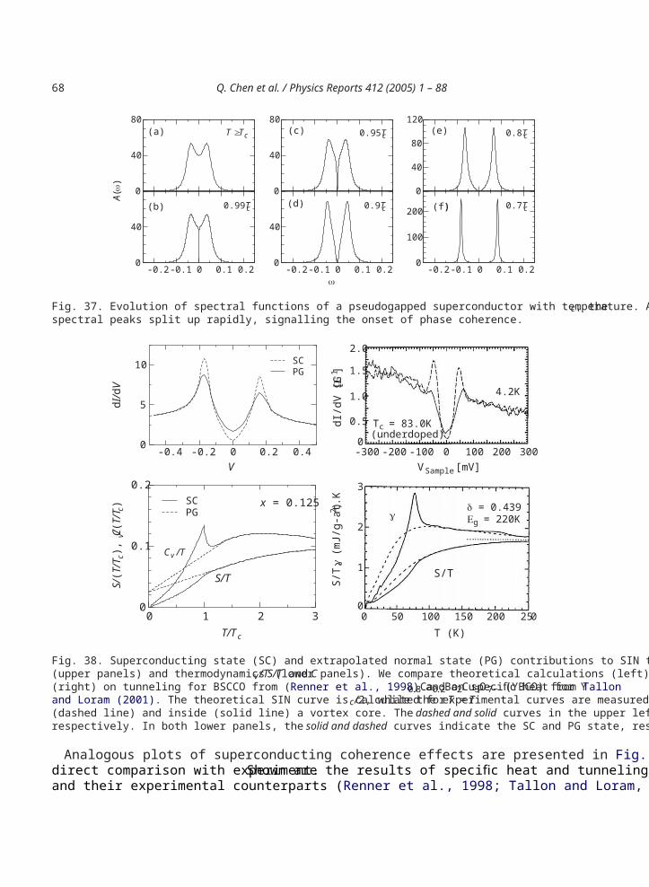
68 Q. Chen et al. / Physics Reports 412 (2005) 1 – 88
0
40
80
-0.2 -0.1 0 0.1 0.20
40
0
40
80
-0.2 -0.1 0 0.1 0.2
0
40
0
40
80
120
-0.2 -0.1 0 0.1 0.20
100
200
A(ω
)
T ≥Tc
0.99Tc
0.95Tc
0.9Tc 0.7Tc
0.8Tc(a)
(b)
(c)
(d)
(e)
(f)
ω
Fig. 37. Evolution of spectral functions of a pseudogapped superconductor with temperature. As soon as T drops belowTc, thespectral peaks split up rapidly, signalling the onset of phase coherence.
-0.4 -0.2 0 0.2 0.4V
0
5
10
dI/d
V
SCPG
0 1 2T/Tc
0
0.1
0.2
S/(T
/Tc)
, Cv/
(T/T
c)
SCPG
S/T
Cv /T
x = 0.125
2.0
1.5
1.0
0.5
0-300 -200 -100 0 100 200 300
VSample [mV]
3
2
1
00 50 100 150 200 250
T (K)
dI/d
V [G
Ω-1
]
Tc = 83.0K(underdoped)
4.2K
δ = 0.439Εg = 220Kγ
S/T
3
S/T,
γ (m
J/g-
at.K
2 )
Fig. 38. Superconducting state (SC) and extrapolated normal state (PG) contributions to SIN tunneling characteristics d I /dV(upper panels) and thermodynamicsS/T and Cv/T (lower panels). We compare theoretical calculations (left) with experiments(right) on tunneling for BSCCO from (Renner et al., 1998) and on specific heat for Y0.8Ca0.2Ba2Cu3O7− (YBCO) from Tallonand Loram (2001). The theoretical SIN curve is calculated for T = Tc/ 2, while the experimental curves are measured outside(dashed line) and inside (solid line) a vortex core. The dashed and solid curves in the upper left panel are for SC and PG state,respectively. In both lower panels, the solid and dashed curves indicate the SC and PG state, respectively.
Analogous plots of superconducting coherence effects are presented in Fig. 38 in the context of moredirect comparison with experiment. Shown are the results of specific heat and tunneling calculationsand their experimental counterparts (Renner et al., 1998; Tallon and Loram, 2001). The latter measures,
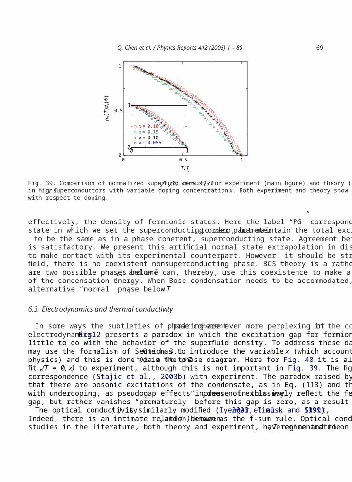
Q. Chen et al. / Physics Reports 412 (2005) 1 – 88 69
0 0.5 1
T/Tc
0
0.5
1
ρ s(T
)/ρs(0
)
00
1
x = 0.18x = 0.15x = 0.10x = 0.055
1
Fig. 39. Comparison of normalized superfluid density s/ s(0) versus T /Tc for experiment (main figure) and theory (inset)in high Tc superconductors with variable doping concentration x. Both experiment and theory show a quasi-universal behaviorwith respect to doping.
effectively, the density of fermionic states. Here the label “PG” corresponds to an extrapolated normalstate in which we set the superconducting order parameter sc to zero, but maintain the total excitation gap
to be the same as in a phase coherent, superconducting state. Agreement between theory and experimentis satisfactory. We present this artificial normal state extrapolation in discussing thermodynamics in orderto make contact with its experimental counterpart. However, it should be stressed that in zero magneticfield, there is no coexistent nonsuperconducting phase. BCS theory is a rather special case in which thereare two possible phases belowTc, and one can, thereby, use this coexistence to make a reasonable estimateof the condensation energy. When Bose condensation needs to be accommodated, there seems to be noalternative “normal” phase below Tc.
6.3. Electrodynamics and thermal conductivity
In some ways the subtleties of phase coherent pairing are even more perplexing in the context ofelectrodynamics. Fig. 12 presents a paradox in which the excitation gap for fermions appears to havelittle to do with the behavior of the superfluid density. To address these data (Stajic et al., 2003b) onemay use the formalism of Section 3.1. One has to introduce the variable x (which accounts for Mottphysics) and this is done via a fit to T∗(x) in the phase diagram. Here for Fig. 40 it is also necessary tofit s(T = 0, x) to experiment, although this is not important in Fig. 39. The figures show a reasonablecorrespondence (Stajic et al., 2003b) with experiment. The paradox raised by Fig. 12 is resolved by notingthat there are bosonic excitations of the condensate, as in Eq. (113) and that these become more markedwith underdoping, as pseudogap effects increase. In this way s does not exclusively reflect the fermionicgap, but rather vanishes “prematurely” before this gap is zero, as a result of pair excitations.
The optical conductivity ( ) is similarly modified (Iyengar et al., 2003; Timusk and Statt, 1999).Indeed, there is an intimate relation between s and ( ) known as the f-sum rule. Optical conductivitystudies in the literature, both theory and experiment, have concentrated on the low , T regime and the
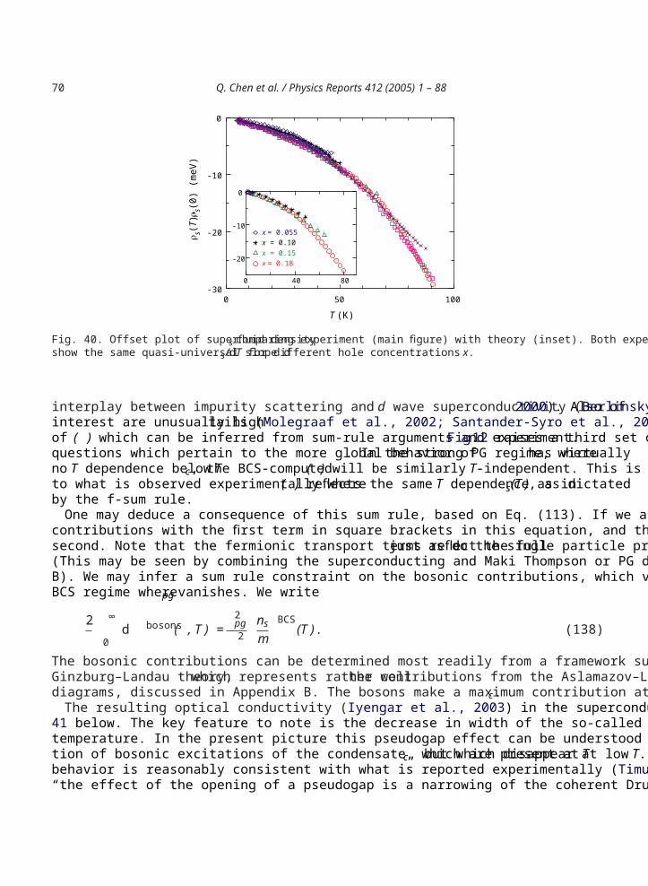
70 Q. Chen et al. / Physics Reports 412 (2005) 1 – 88
0 50 100
T (K)
-30
-20
-10
0
ρ s(T)-ρ s(0
) (m
eV)
0 40 80
-20
-10
0
x = 0.055x = 0.10x = 0.15x = 0.18
Fig. 40. Offset plot of superfluid density s comparing experiment (main figure) with theory (inset). Both experiment and theoryshow the same quasi-universal slope d s/dT for different hole concentrations x.
interplay between impurity scattering and d wave superconductivity (Berlinsky et al., 2000). Also ofinterest are unusually high tails (Molegraaf et al., 2002; Santander-Syro et al., 2003) in the real partof ( ) which can be inferred from sum-rule arguments and experiment. Fig. 12 raises a third set ofquestions which pertain to the more global behavior of . In the strong PG regime, where has virtuallyno T dependence below Tc, the BCS-computed ( ) will be similarly T-independent. This is in contrastto what is observed experimentally where ( ) reflects the same T dependence as in s(T ), as dictatedby the f-sum rule.
One may deduce a consequence of this sum rule, based on Eq. (113). If we associate the fermioniccontributions with the first term in square brackets in this equation, and the bosonic contributions with thesecond. Note that the fermionic transport terms reflect the full just as do the single particle properties.(This may be seen by combining the superconducting and Maki Thompson or PG diagrams in AppendixB). We may infer a sum rule constraint on the bosonic contributions, which vanish as expected in theBCS regime where pg vanishes. We write
2 ∞
0d bosons( , T ) =
2pg2
nsm
BCS(T ) . (138)
The bosonic contributions can be determined most readily from a framework such as time dependentGinzburg–Landau theory, which represents rather well the contributions from the Aslamazov–Larkindiagrams, discussed in Appendix B. The bosons make a maximum contribution at Tc.
The resulting optical conductivity (Iyengar et al., 2003) in the superconducting state is plotted in Fig.41 below. The key feature to note is the decrease in width of the so-called Drude peak with decreasingtemperature. In the present picture this pseudogap effect can be understood as coming from the contribu-tion of bosonic excitations of the condensate, which are present atTc, but which disappear at low T. Thisbehavior is reasonably consistent with what is reported experimentally (Timusk and Statt, 1999), where“the effect of the opening of a pseudogap is a narrowing of the coherent Drude peak at low frequency”.
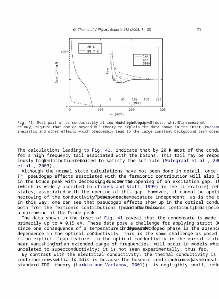
Q. Chen et al. / Physics Reports 412 (2005) 1 – 88 71
0 100 200 300 ω [meV]
0
4000R
e σ
[Ω-1
cm
-1]
20 K88.7 K
150100 2000
10K
300K65K
Re σ
50E (meV)
Fig. 41. Real part of ac conductivity at low and high T below Tc. Here pseudogap effects, which insure that (T ) ≈constantbelow Tc, require that one go beyond BCS theory to explain the data shown in the inset (Puchkov et al., 1996). In the theory,inelastic and other effects which presumably lead to the large constant background term observed in the data have been ignored.
The calculations leading to Fig. 41, indicate that by 20 K most of the conductivity is fermionic exceptfor a high frequency tail associated with the bosons. This tail may be responsible in part for the anoma-lously high contributions to required to satisfy the sum rule (Molegraaf et al., 2002; Santander-Syroet al., 2003).
Although the normal state calculations have not been done in detail, once the temperature is less thanT∗, pseudogap effects associated with the fermionic contribution will also lead to a progressive narrowingin the Drude peak with decreasing T, down toTc, due to the opening of an excitation gap. This mechanism(which is widely ascribed to (Timusk and Statt, 1999) in the literature) reflects longer lived electronicstates, associated with the opening of this gap. However, it cannot be applied to explain the progressivenarrowing of the conductivity peaks, once (T )becomes temperature independent, as is the case at low T.In this way, one can see that pseudogap effects show up in the optical conductivity of underdoped samples,both from the fermionic contributions (near and below T∗) and the bosonic contributions (below Tc) asa narrowing of the Drude peak.
The data shown in the inset of Fig. 41 reveal that the condensate is made from frequency contributionsprimarily up to ≈ 0.15 eV. These data pose a challenge for applying strict BCS theory to this problem,since one consequence of a temperature independent in the underdoped phase is the absence of Tdependence in the optical conductivity. This is the same challenge as posed by Fig. 12. Strikingly thereis no explicit “gap feature” in the optical conductivity in the normal state. Such a gap feature, that is anear vanishing of for an extended range of frequencies, will occur in models where the pseudogap isunrelated to superconductivity; it is not seen experimentally, thus far.
By contrast with the electrical conductivity, the thermal conductivity is dominated by the fermioniccontributions at essentially all T. This is because the bosonic contribution to the heat current (as instandard TDGL theory (Larkin and Varlamov, 2001)), is negligibly small, reflecting the low energy scales
72 Q. Chen et al. / Physics Reports 412 (2005) 1 – 88
of the bosons. Thermal conductivity, experiments (Sutherland et al., 2003) in the highTc superconductorsprovide some of the best evidence for the presence of fermionic d-wave quasiparticles belowTc. In contrastto the ac conductivity, here one sees a universal low T limit (Lee, 1993), and there is little to suggest thatsomething other than conventional d-wave BCS physics is going on here. This cannot quite be the casehowever, since in the pseudogap regime, the temperature dependence of the fermionic excitation gap ishighly anomalous, as shown in Fig. 3, compared to the BCS analogue.
6.4. Thermodynamics and pair-breaking effects
The existence of noncondensed pair states below Tc affects thermodynamics, in the same way thatelectrodynamics is affected, as discussed above. Moreover, one can predict (Chen et al., 2000) that theq2 dispersion will lead to ideal Bose gas power laws in thermodynamical and transport properties. Thesewill be present in addition to the usual power laws or (for s-wave) exponential temperature dependencesassociated with the fermionic quasiparticles. Note that the q2 dependence reflects the spatial extent pg,of the composite pairs, and this size effect has no natural counterpart in true Bose systems. It should bestressed that numerical calculations show that these pair masses, as well as the residue Z are roughly Tindependent constants at low T. As a result, Eq. (94) implies that 2
pg = 2(T ) − 2sc(T ) ∝ T3/2.
The consequences of these observations can now be listed (Chen et al., 2000). For a quasi-two dimen-sional system, Cv/T will appear roughly constant at the lowest temperatures, although it vanishes strictlyat T = 0 as T 1/2. The superfluid density s(T )will acquire a T 3/2 contribution in addition to the usualfermionic terms. By contrast, for spin singlet states, there is no explicit pair contribution to the Knightshift. In this way the low T Knight shift reflects only the fermions and exhibits a scaling with T / (0) atlow temperatures. Experimentally, in the cuprates, one usually sees a finite low T contribution to Cv/T .A Knight shift scaling is seen. Finally, also observed is a deviation from the predicted d-wave linear inT power law in s. The new power laws in Cv and s are conventionally attributed to impurity effects,where s ∝ T 2, and Cv/T ∝ const. Experiments are not yet at a stage to clearly distinguish betweenthese two alternative explanations.
Pair-breaking effects are viewed as providing important insight into the origin of the cuprate pseudogap.Indeed, the different pair-breaking sensitivities of T∗and Tc are usually proposed to support the notionthat the pseudogap has nothing to do with superconductivity. To counter this inference, a detailed set ofstudies was conducted, (based on the BEC–BCS scenario), of pair-breaking in the presence of impurities(Chen and Schrieffer, 2002; see also Kao et al., 2002) and of magnetic fields (Kao et al., 2001). Thesestudies make it clear that the superconducting coherence temperature Tc is far more sensitive to pair-breaking than is the pseudogap onset temperatureT∗. Indeed, the phase diagram of Fig. 35 which mirrorsits experimental counterpart, shows the very different, even competing nature of T∗and Tc, despite thefact that both arise from the same pairing correlations.
6.5. Anomalous normal state transport: Nernst and other precursor transport contributions
Much attention is given to the anomalous behavior of the Nernst coefficient in the cuprates (Xu et al.,2000). This coefficient is rather simply related to the transverse thermoelectric coefficient xy which isplotted in Fig. 13. In large part, the origin of the excitement in the literature stems from the fact that theNernst coefficient behaves smoothly through the superconducting transition. Below Tc it is understoodto be associated with superconducting vortices. Above Tc if the system were a Fermi liquid, there are
Q. Chen et al. / Physics Reports 412 (2005) 1 – 88 73
arguments to prove that the Nernst coefficient should be essentially zero. Hence the observation of anonnegligible Nernst contribution has led to the picture of normal state vortices.
Another way to view these data is that there are bosonic degrees of freedom present in the normal state, asin the BCS–BEC crossover approach. To describe this dynamics we begin with the TDGL scheme outlinedin Section 1.8.1. This formalism must be modified somewhat however. When “pre-formed” pairs arepresent at temperatures T∗high compared to Tc, the classical bosonic fields of conventional TDGL mustbe replaced by their quantum counterparts (Tan and Levin, 2004). We investigate this fairly straightforwardextension of TDGL in the next sub-section, and subsequently explore the resulting implications fortransport.
6.5.1. Quantum extension of TDGLTo make progress on the quantum analogue of TDGL we study a Hamiltonian describing bosons
coupled to a particle reservoir of fermion pairs. The latter are addressed in a quantum mechanical fashion.Our treatment of the reservoir has strong similarities to the approach of Caldeira and Leggett (1983).These bosons are in the presence of an electromagnetic field, which interacts with the fermion pairs ofthe reservoir as well, since they have charge e∗= 2e. For simplicity we assume that the fermions aredispersionless. This Hamiltonian is given by
H =lm
εlm†l (t )exp(−ie∗Clm(t )) m(t )
+l
e∗ † +i l
(ai + e∗ )w†i wi + i
†wi + ∗i w
†i
+i l
(bi − e∗ )v†i vi + i
†v†i + ∗
i vi . (139)
Here εlm is the hopping matrix element for the bosons. Clm(t )is the usual phase factor associatedwith the vector potential. Annihilation operators for the reservoir, wi and vi (with infinitesimal couplingconstants i and i ), represent positive and negative frequencies respectively and need to be treatedseparately. The energies ai and bi of the reservoir are both positive.
The bosonic propagatorT (k, ) can be exactly computed from the equations of motion. HereA(k, )=Re2iT (k, ) is the boson spectral function, and
T (k, ) ≡ − ε(k) − 1( ) + i2 2( )
−1. (140)
We have
2( ) ≡ 2i
| i |2 ( − ai) −2i
| i |2 ( + bi) , (141)
with 1( ) defined by a Kramers Kronig transform.The reservoir parameters ai , bi , i and i which are of no particular interest, are all subsumed into the
boson self energy 2( ). From this point forward we may ignore these quantities in favor of the bosonself energy. We reiterate that this theory makes an important simplification, that the reservoir pairs haveno dispersion. For this case one can solve for the exact transport coefficients.
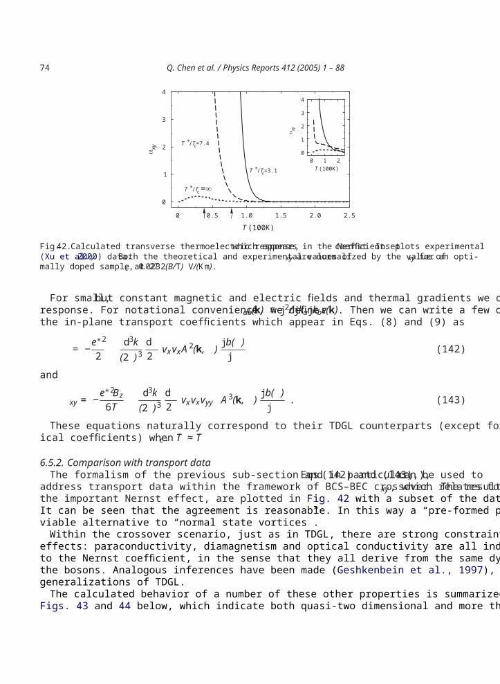
74 Q. Chen et al. / Physics Reports 412 (2005) 1 – 88
0 0.5 1.0 1.5 2.0 2.5
0
1
2
3
4
T (100K)
T (100K)T ∗/Tc=3.1
T ∗/Tc=7.4
0 1 20
1
2
3
4
T ∗/Tc =∞
αxy
α xy
Fig. 42. Calculated transverse thermoelectric response, which appears in the Nernst coefficient. Inset plots experimental(Xu et al., 2000) data. Both the theoretical and experimental values of xy are normalized by the value of xy for an opti-mally doped sample at 2Tc, 0.0232(B/ T) V/(K m).
For small, but constant magnetic and electric fields and thermal gradients we obtain the linearizedresponse. For notational convenience, we define vab(k) ≡ j 2/ j kaj kbε(k). Then we can write a few ofthe in-plane transport coefficients which appear in Eqs. (8) and (9) as
= −e∗2
2d3k
(2 )3d2
vxvxA2(k, ) j b( )j (142)
and
xy = −e∗2Bz6T
d3k(2 )3
d2
vxvxvyy A3(k, ) j b( )j . (143)
These equations naturally correspond to their TDGL counterparts (except for different phenomenolog-ical coefficients) when T ≈ Tc.
6.5.2. Comparison with transport dataThe formalism of the previous sub-section and in particular, Eqs. (142) and (143),), can be used to
address transport data within the framework of BCS–BEC crossover. The results for xy, which relates tothe important Nernst effect, are plotted in Fig. 42 with a subset of the data plotted in the upper right inset.It can be seen that the agreement is reasonable. In this way a “pre-formed pair” picture is, at present, aviable alternative to “normal state vortices”.
Within the crossover scenario, just as in TDGL, there are strong constraints on other precursor transporteffects: paraconductivity, diamagnetism and optical conductivity are all indirectly or directly connectedto the Nernst coefficient, in the sense that they all derive from the same dynamical equation of motion forthe bosons. Analogous inferences have been made (Geshkenbein et al., 1997), based on similar bosonicgeneralizations of TDGL.
The calculated behavior of a number of these other properties is summarized (Tan and Levin, 2004) inFigs. 43 and 44 below, which indicate both quasi-two dimensional and more three dimensional behavior.
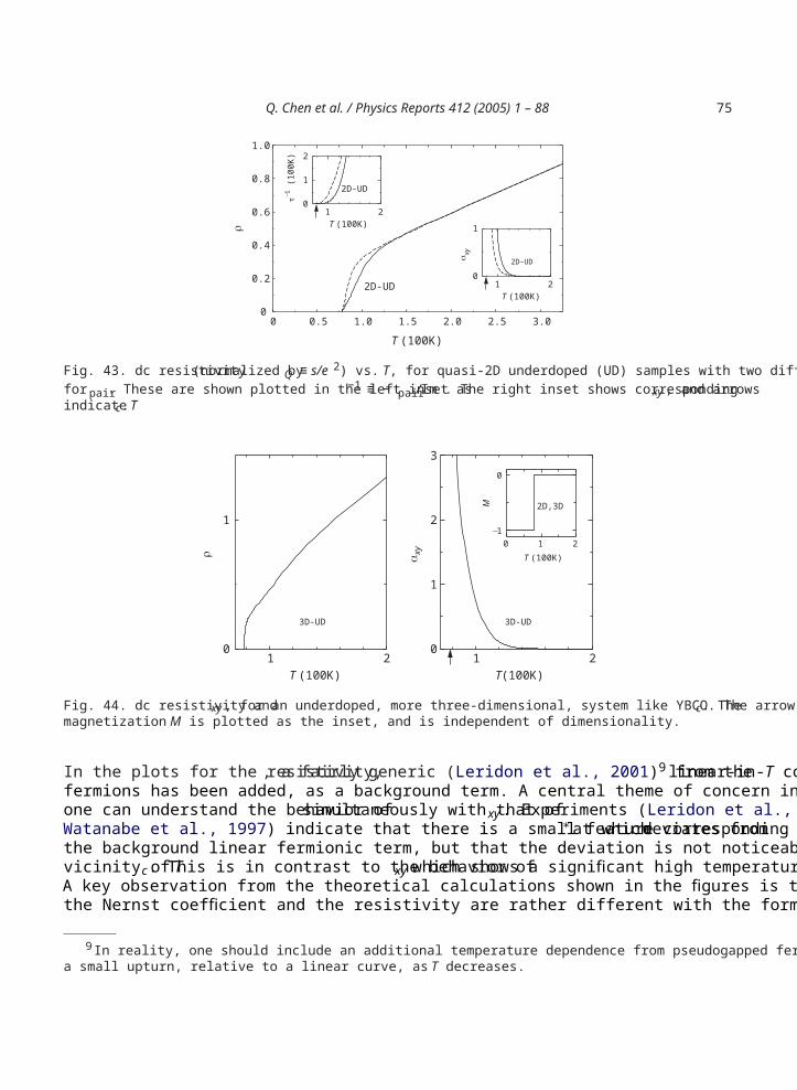
Q. Chen et al. / Physics Reports 412 (2005) 1 – 88 75
0 0.5 1.0 1.5 2.0 2.5 3.00
0.2
0.4
0.6
0.8
1.0
T (100K)
2D-UD
1 20
1
2
T (100K)
τ−1 (1
00K
)
2D-UD
1 20
1
T (100K)
α xy
2D-UD
ρ
Fig. 43. dc resistivity (normalized by Q ≡ s/e2) vs. T, for quasi-2D underdoped (UD) samples with two different formsfor pair. These are shown plotted in the left inset as −1 ≡ − pair/ Im . The right inset shows corresponding xy, and arrowsindicate Tc.
1 20
1
T (100K)
3D-UD
1 20
1
2
3
T(100K)
αxy
3D-UD
0 1 2−1
0
T (100K)
M 2D,3D
ρ
Fig. 44. dc resistivity and xy, for an underdoped, more three-dimensional, system like YBCO. The arrow indicates Tc. Themagnetization M is plotted as the inset, and is independent of dimensionality.
In the plots for the resistivity, , a fairly generic (Leridon et al., 2001) linear-in-T contribution9 from thefermions has been added, as a background term. A central theme of concern in the literature is whetherone can understand the behavior of simultaneously with that of xy. Experiments (Leridon et al., 2001;Watanabe et al., 1997) indicate that there is a small feature corresponding toT∗at which deviates fromthe background linear fermionic term, but that the deviation is not noticeably large except in the immediatevicinity of Tc. This is in contrast to the behavior of xy which shows a significant high temperature onset.A key observation from the theoretical calculations shown in the figures is that the onset temperatures forthe Nernst coefficient and the resistivity are rather different with the former being considerably higher
9 In reality, one should include an additional temperature dependence from pseudogapped fermions which presumably hasa small upturn, relative to a linear curve, as T decreases.
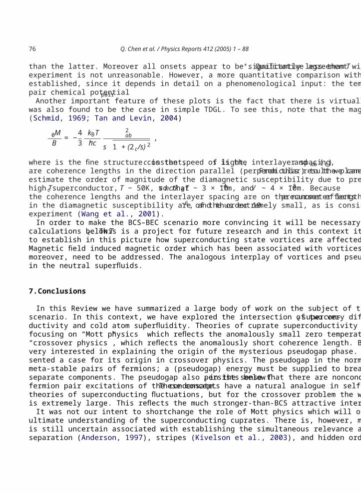
76 Q. Chen et al. / Physics Reports 412 (2005) 1 – 88
than the latter. Moreover all onsets appear to be significantly less than T∗. Qualitative agreement withexperiment is not unreasonable. However, a more quantitative comparison with experiment has not beenestablished, since it depends in detail on a phenomenological input: the temperature dependence of thepair chemical potential pair.
Another important feature of these plots is the fact that there is virtually no diamagnetic precursor, aswas also found to be the case in simple TDGL. To see this, note that the magnetization can be written(Schmid, 1969; Tan and Levin, 2004)
0MB
= −43
kBThc
2ab
s 1 + (2 c/s)2,
where is the fine structure constant, c is the speed of light, s is the interlayer spacing, and ab ( c)are coherence lengths in the direction parallel (perpendicular) to the planes. From this result we canestimate the order of magnitude of the diamagnetic susceptibility due to preformed pairs. For a typicalhigh Tc superconductor, T ∼ 50K, so that ≡ hc/kBT ∼ 3 × 10⁻⁴m, and / ∼ 4 × 10⁻²m. Becausethe coherence lengths and the interlayer spacing are on the nanometer length scale, precursor effectsin the diamagnetic susceptibility are of the order 10 −6, and thus extremely small, as is consistent withexperiment (Wang et al., 2001).
In order to make the BCS–BEC scenario more convincing it will be necessary to take these transportcalculations belowTc. This is a project for future research and in this context it will ultimately be importantto establish in this picture how superconducting state vortices are affected by the persistent pseudogap.Magnetic field induced magnetic order which has been associated with vortices (Lake et al., 2002) will,moreover, need to be addressed. The analogous interplay of vortices and pseudogap will also be of interestin the neutral superfluids.
7. Conclusions
In this Review we have summarized a large body of work on the subject of the BCS–BEC crossoverscenario. In this context, we have explored the intersection of two very different fields: highTc supercon-ductivity and cold atom superfluidity. Theories of cuprate superconductivity can be crudely classified asfocusing on “Mott physics” which reflects the anomalously small zero temperature superfluid density and“crossover physics”, which reflects the anomalously short coherence length. Both schools are currentlyvery interested in explaining the origin of the mysterious pseudogap phase. In this Review we have pre-sented a case for its origin in crossover physics. The pseudogap in the normal state can be associated withmeta-stable pairs of fermions; a (pseudogap) energy must be supplied to break these pairs apart into theirseparate components. The pseudogap also persists below Tc in the sense that there are noncondensedfermion pair excitations of the condensate. These concepts have a natural analogue in self consistenttheories of superconducting fluctuations, but for the crossover problem the width of the “critical region”is extremely large. This reflects the much stronger-than-BCS attractive interaction.
It was not our intent to shortchange the role of Mott physics which will obviously be of importance in ourultimate understanding of the superconducting cuprates. There is, however, much in this regard whichis still uncertain associated with establishing the simultaneous relevance and existence of spin-chargeseparation (Anderson, 1997), stripes (Kivelson et al., 2003), and hidden order parameters (Chakravarty
Q. Chen et al. / Physics Reports 412 (2005) 1 – 88 77
et al., 2001). What we do have in hand, though, is a very clear experimental picture of an extremelyunusual superconductor in which superconductivity seems to evolve gradually from above Tc to below.We have in this Review tried to emphasize the common ground between high Tc superconductors andultracold superfluids. These Mott issues may nevertheless, set the agenda for future cold atom studies offermions in optical lattices (Hofstetter et al., 2002).
The recent discovery of superfluidity in cold fermion gases opens the door to a new set of fascinatingproblems in condensed matter physics. Unlike the bosonic system, there is no ready-made counterpartof Gross Pitaevskii theory. A new mean field theory which goes beyond BCS and encompasses BEC insome form or another will have to be developed in concert with experiment. As of this writing, there arefour experiments where the simple mean field theory discussed in this review is in reasonable agreementwith the data. These are the collective mode studies over the entire range of accessible magnetic fields(Heiselberg, 2004b; Hu et al., 2004). In addition in the unitary regime, RF spectroscopy-based pairinggap studies (Kinnunen et al., 2004a), as well as density profile (Stajic et al., 2005a) and thermodynamicstudies (Kinast et al., 2005) all appear to be compatible with this theory.
The material in this Review is viewed as the first of many steps in a long process. It was felt, however,that some continuity should be provided from another community which has addressed and helped todevelop the BCS–BEC crossover, since the early 1990s when the early signs of the cuprate pseudogapwere beginning to appear. As of this writing, it appears likely that the latest experiments on cold atomsprobe a counterpart to this pseudogap regime. That is, on both sides, but near the resonance, fermionsform in long lived metastable pair states at higher temperatures than those at which they Bose condense.
Acknowledgements
We gratefully acknowledge the help of our many close collaborators over the years: J. Maly, B. Jankó,I. Kosztin, Y.-J. Kao and A. Iyengar. We also thank our colleagues T.R. Lemberger, B.R. Boyce, J.N.Milstein, M.L. Chiofalo and M.J. Holland, and most recently, J.E. Thomas, J. Kinast, and A. Turlapov.This work was supported by NSF-MRSEC Grant No. DMR-0213765 (JS,ST and KL), NSF Grant No.DMR0094981 and JHU-TIPAC (QC).
Appendix A. Derivation of the T = 0 variational conditions
The ground state wavefunction is given by
¯0 = e− 2/2+ b†0 |0 ⊗k(uk + vka†
ka†−k)|0 . (A.1)
Thus one has three variational parameters , uk, vk with normalization condition u2k + v2
k = 1. We candefine k such that uk = sin k and vk = cos k, so that we have only two variational parameters,and k.
We then have
¯0|H − N| ¯0 = (− 2 ) 2 + 2k
( k − )v2k + 2U
k,kukvkuk vk + 2g
kukvk ,
where we have chosen k = 1 in Eq. (11) for simplicity.
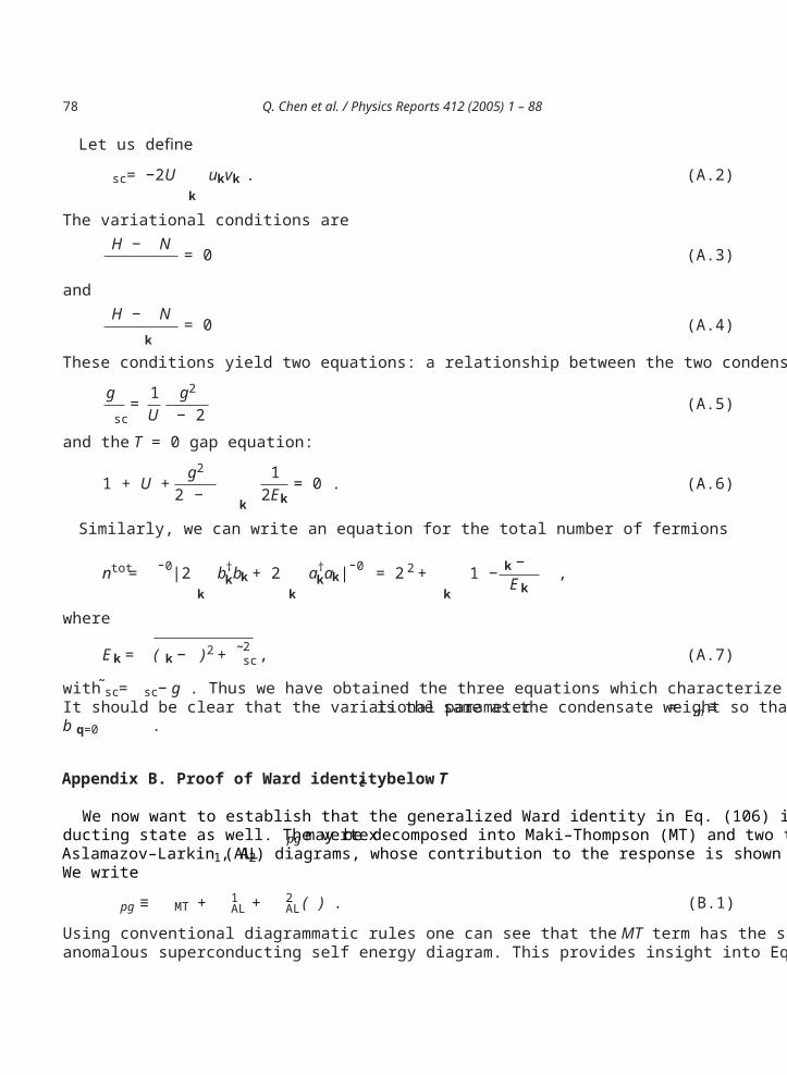
78 Q. Chen et al. / Physics Reports 412 (2005) 1 – 88
Let us define
sc = −2Uk
ukvk . (A.2)
The variational conditions areH − N = 0 (A.3)
andH − N
k= 0 (A.4)
These conditions yield two equations: a relationship between the two condensates
gsc
= 1U
g2
− 2(A.5)
and the T = 0 gap equation:
1 + U + g2
2 −k
12Ek
= 0 . (A.6)
Similarly, we can write an equation for the total number of fermions
ntot = ¯0|2k
b†kbk + 2
ka†
kak| ¯0 = 2 2 +k
1 − k −Ek
,
where
Ek = ( k − )2 + ˜2sc , (A.7)
with ˜sc = sc − g . Thus we have obtained the three equations which characterize the system atT = 0.It should be clear that the variational parameter is the same as the condensate weight so that = m ≡b q=0 .
Appendix B. Proof of Ward identitybelow Tc
We now want to establish that the generalized Ward identity in Eq. (106) is correct for the supercon-ducting state as well. The vertex pg may be decomposed into Maki–Thompson (MT) and two types ofAslamazov–Larkin (AL1, AL2) diagrams, whose contribution to the response is shown here in Fig. 45b.We write
pg ≡ MT + 1AL + 2
AL( ) . (B.1)
Using conventional diagrammatic rules one can see that the MT term has the same sign reversal as theanomalous superconducting self energy diagram. This provides insight into Eq. (107). Here, however,
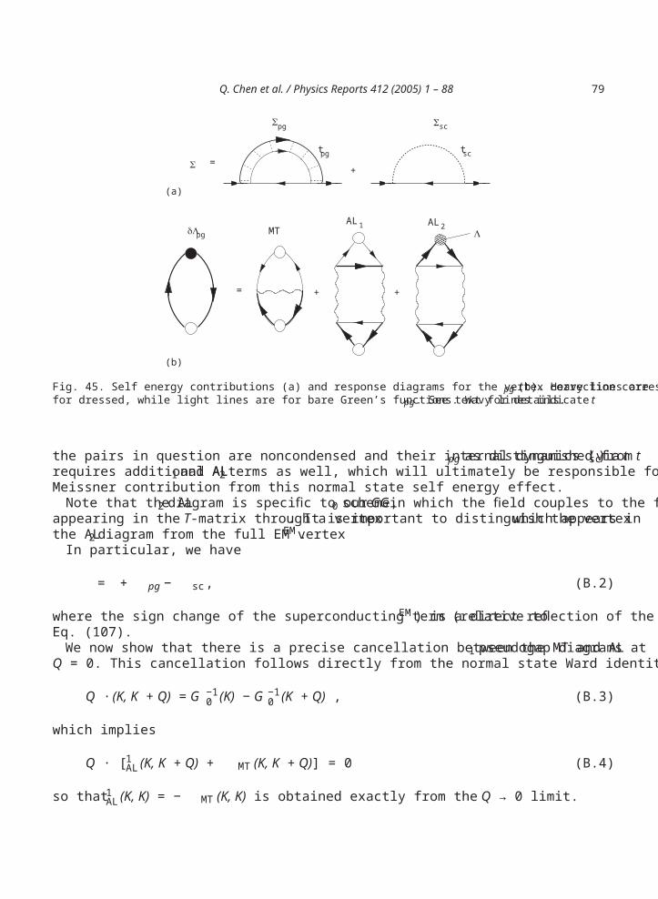
Q. Chen et al. / Physics Reports 412 (2005) 1 – 88 79
AL1 AL2 δΛpg
tpg tsc
Σsc
MT
+ +
=
Λ
=
+Σ
Σpg
(a)
(b)
Fig. 45. Self energy contributions (a) and response diagrams for the vertex correction corresponding topg (b). Heavy lines arefor dressed, while light lines are for bare Green’s functions. Wavy lines indicatetpg. See text for details.
the pairs in question are noncondensed and their internal dynamics (via tpg as distinguished from tsc)requires additional AL1 and AL2 terms as well, which will ultimately be responsible for the absence of aMeissner contribution from this normal state self energy effect.
Note that the AL 2 diagram is specific to our GG0 scheme, in which the field couples to the full Gappearing in the T-matrix through a vertex . It is important to distinguish the vertex which appears inthe AL2 diagram from the full EM vertex EM.
In particular, we have
= + pg − sc , (B.2)
where the sign change of the superconducting term (relative to EM) is a direct reflection of the sign inEq. (107).
We now show that there is a precise cancellation between the MT and AL 1 pseudogap diagrams atQ =0. This cancellation follows directly from the normal state Ward identity
Q · (K, K + Q) = G−10 (K) − G−1
0 (K + Q) , (B.3)
which implies
Q · [ 1AL(K, K + Q) + MT(K, K + Q)] =0 (B.4)
so that 1AL(K, K) = − MT(K, K) is obtained exactly from the Q → 0 limit.
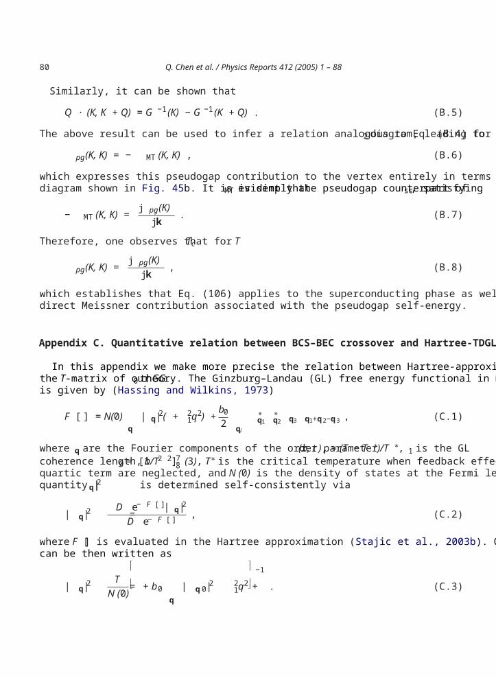
80 Q. Chen et al. / Physics Reports 412 (2005) 1 – 88
Similarly, it can be shown that
Q · (K, K + Q) = G−1(K) − G−1(K + Q) . (B.5)
The above result can be used to infer a relation analogous to Eq. (B.4) for the AL2 diagram, leading to
pg(K, K) = − MT(K, K) , (B.6)
which expresses this pseudogap contribution to the vertex entirely in terms of the Maki–Thompsondiagram shown in Fig. 45b. It is evident that MT is simply the pseudogap counterpart of sc, satisfying
− MT(K, K) = j pg(K)j k
. (B.7)
Therefore, one observes that for T ⩽Tc
pg(K, K) = j pg(K)j k
, (B.8)
which establishes that Eq. (106) applies to the superconducting phase as well. As expected, there is nodirect Meissner contribution associated with the pseudogap self-energy.
Appendix C. Quantitative relation between BCS–BEC crossover and Hartree-TDGL
In this appendix we make more precise the relation between Hartree-approximated TDGL theory andthe T-matrix of our GG0 theory. The Ginzburg–Landau (GL) free energy functional in momentum spaceis given by (Hassing and Wilkins, 1973)
F [ ] = N(0)q
| q|2( + 21q2) + b0
2 qi
∗q1
∗q2 q3 q1+q2−q3 , (C.1)
where q are the Fourier components of the order parameter (r, t ), = (T − T∗)/T ∗, 1 is the GLcoherence length, b0 = [1/T 2 2]7
8 (3), T∗ is the critical temperature when feedback effects from thequartic term are neglected, and N(0) is the density of states at the Fermi level in the normal state. Thequantity | q|2 is determined self-consistently via
| q|2 =D e− F [ ]| q|2D e− F [ ] , (C.2)
where F [ ] is evaluated in the Hartree approximation (Stajic et al., 2003b). Our self consistency conditioncan be then written as
| q|2 =TN(0)
+ b0q
| q 0|2 +21q2
−1
. (C.3)
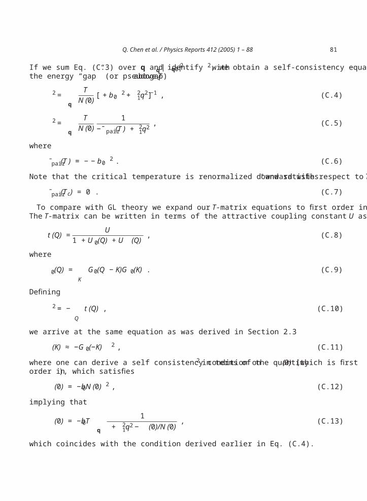
Q. Chen et al. / Physics Reports 412 (2005) 1 – 88 81
If we sum Eq. (C.3) over q and identify q | q0|2 with 2, we obtain a self-consistency equation forthe energy “gap” (or pseudogap) above Tc
2 =q
TN(0) [ + b0
2 + 21q2]−1 , (C.4)
2 =q
TN(0)
1−¯pair(T ) + 2
1q2, (C.5)
where
pair(T ) = −− b02 . (C.6)
Note that the critical temperature is renormalized downward with respect to T∗and satisfies
pair(Tc) =0 . (C.7)
To compare with GL theory we expand our T-matrix equations to first order in the self energy correction.The T-matrix can be written in terms of the attractive coupling constant U as
t (Q) = U1 + U 0(Q) + U (Q) , (C.8)
where
0(Q) =K
G0(Q − K)G0(K) . (C.9)
Defining
2 = −Q
t (Q), (C.10)
we arrive at the same equation as was derived in Section 2.3
(K) ≈ −G0(−K) 2 , (C.11)
where one can derive a self consistency condition on 2 in terms of the quantity (0) (which is firstorder in ), which satisfies
(0) = −b0N(0) 2 , (C.12)
implying that
(0) = −b0Tq
1+ 2
1q2 − (0)/N (0), (C.13)
which coincides with the condition derived earlier in Eq. (C.4).
82 Q. Chen et al. / Physics Reports 412 (2005) 1 – 88
Appendix D. Convention and notation
D.1. Notation
We follow standard notations as much as possible. They are summarized below.
EF Fermi energykF Fermi momentumh Planck constantkB Boltzmann constantc speed of lighte electron chargeTc critical temperature for (superfluid/superconducting)
phase transitionT∗ pair formation or pseudogap onset temperatureT temperature
, pair, B Fermionic, pair and bosonic chemical potential, respec-tivelyFermionic excitation gap
sc superconducting/superfluid order parameterpg pseudogap
Four vector K ≡ (i n, k), K ≡ T n k, where n = (2n +1) T is the odd (fermionic) Matsubarafrequency.Four vector Q ≡ ( i n, q), Q ≡ T n q, where n = 2n T is the even (bosonic) Matsubarafrequency.f (x) =1/(ex/kBT + 1) Fermi distribution functionb(x) =1/(ex/kBT − 1) Bose distribution functionG(K) , G0(K) full and bare Green’s functions for fermionsD(Q) , D0(Q) full and bare Green’s functions for Feshbach bosons(K) , B(Q) self energy of fermions and bosons, respectively(Q) pair susceptibility
t (Q) T-matrix, bare and full vertex, respectively, 0 magnetic detuning parameter
as, a∗s S-wave inter-fermion scattering length
U, U0 renormalized and bare strength of the attractive inter-action between fermions in the open-channel. U0 ∝as( = +∞)
Uc critical coupling strength at which the two-body scat-tering length diverges
A = ( , A) four vector potentialJ = ( , J) four currentK (Q) electromagnetic response kernel
Q. Chen et al. / Physics Reports 412 (2005) 1 – 88 83
k = k2/2m bare fermion dispersion in free spacek = k − bare fermion dispersion measured from chemical po-
tentialEk Bogoliubov quasiparticle dispersionu2
k = 12 (1 + k/E k), v2
k = 12(1 − k/E k) coherence factor as given in BCS theory
ntot = n +2(nb + nb0) total, fermion, finite momentum boson, condensed bo-son density, respectively
V (r) =12m 2r2 harmonic trap potential
We use alphabetic ordering when multiple authors appear together.We always refer to the absolute value when we refer to the interaction parameters U, U0, g, g0 as
increasing or decreasing.
D.2. Convention for units
Throughout this Review, we use the convention for units where it is not explicitly spelled out:
h = kB = c =1 .
EF = TF = kF = 2m =1 .
In a harmonic trap, EF, TF and kF are defined by the noninteracting Fermi gas with the same totalparticle number N. EF = h (3N)1/3. We further take the Thomas–Fermi radius RTF = 1.
In this convention, the fermion density in a homogeneous gas in three dimensions is n =1/3 2, theharmonic trap frequency = 2, and the total fermion number in a trap is N = 1/24.
In the two-channel model, the units are EF/k 3F for U and U0, and EF/k 3/2
F for g and g0.Our fermionic chemical potential is measured with respect to the bottom of the energy band, which
leads to (i) = EF in the noninteracting limit at T = 0, and (ii) changes sign when the system crossesthe boundary between fermionic and bosonic regimes.
D.3. Abbreviations
BCS Bardeen–Cooper–Schrieffer (theory)BEC Bose–Einstein condensationpg pseudogapsc superconductorAFM antiferromagnetLSCO La1−xSrxCuO4BSCCO Bi2Sr2CaCu2O8+YBCO YBa2Cu3O7−ARPES angle-resolved photoemission spectroscopySTM scan tunneling microscopySIN superconductor–insulator–normal metal (tunnelling junction)TDGL time-dependent Ginzburg–Landau theory
84 Q. Chen et al. / Physics Reports 412 (2005) 1 – 88
FB Feshbach bosonFLEX fluctuation exchangeNSR Noziéres and Schmitt-RinkAB Anderson–BogoliubovTF Thomas–Fermi3D three dimensionsRPA Random phase approximationLDA Local density approximationGP Gross–Pitaevskii (theory)RF Radio frequency (spectroscopy)SI Superconductor–insulator (transition)
References
Aeppli, G., Mason, T.E., Hayden, S.M., Mook, H.A., Kulda, J., 1997a. Science 278 (5342), 1432.Aeppli, G., Mason, T.E., Mook, H.A., Schroeder, A., Hayden, S.M., 1997b. Physica C 231, 282–287.Anderson, P.W., 1997. The Theory of Superconductivity in the High-Tc Cuprate Superconductors. Princeton University Press,
Princeton.Anderson, P.W., Brinkman, W.F., 1973. Phys. Rev. Lett. 30 (1), 1108.Anderson, P.W., Lee, P.A., Randeria, M., Rice, T.M., Trivedi, N., Zhang, F.C., 2004. J. Phys.: Condens. Matter. 16, R755.Ando, Y.G.S., Boebinger, P.A., Kimura, T., Kishio, K., 1995. Phys. Rev. Lett. 75 (25), 4662.Andrenacci, N., Perali, A., Pieri, P., Strinati, G.C., 1999. Phys. Rev. B 60, 12410.Baker, J.G.A., 1999. Phys. Rev. C 60, 054311.Baldo, M., Lombardo, U., Schuck, P., 1995. Phys. Rev. C 52, 975.Bartenstein, M., Altmeyer, A., Riedl, S., Jochim, S., Chin, C., Denschlag, J., Grimm, R., 2004a. Phys. Rev. Lett. 92, 203201.Bartenstein, M., Altmeyer, A., Riedl, S., Jochim, S., Chin, C., Hecke, D., G.R., 2004b. Phys. Rev. Lett. 92, 120401.Baym, G., 1962. Phys. Rev. 127 (4), 1391.Belkhir, L., Randeria, M., 1992. Phys. Rev. B 45 (1), 5087.Benard, P., Chen, L., Tremblay, A.M.S., 1993. Phys. Rev. B 47 (22), 15217.Berlinsky, A., Bonn, D., Harris, R., Kallin, C., 2000. Phys. Rev. B 61 (13), 9088.Bourdel, T., Khaykovich, L., Cubizolles, J., Zhang, J., Chevy, F., Teichmann, M., Tarruell, L., Kokkelmans, S.J., Salomon, C.,
2004. Phys. Rev. Lett. 93, 050401.Bruun, G.M., Baym, G., 2004. Phys. Rev. Lett. 93, 150403.Bruun, G.M., Pethick, C.J., 2004. Phys. Rev. Lett. 92, 140404.Caldeira, A., Leggett, A., 1983. Physica 121A (4), 587.Campuzano, J.C., Norman, M.R., Randeria, M., 2004. Physics of Superconductors, vol. II, Chapter-Photoemission in the High
Tc Superconductors, Springer-Verlag, Springer, Berlin, pp. 167–273.Carlson, E.W., Emery, V.J., Kivelson, S.A., Orgad, D., 2002. Concepts in high temperature superconductivity, preprint; cond-
mat/0206217.Carlson, E.W., Kivelson, S.A., Emery, V.J., Manousakis, E., 1999. Phys. Rev. Lett. 83 (3), 612.Carr, L.D., Shlyapnikov, G.V., Castin, Y., 2004. Phys. Rev. Lett. 92 (15), 150404.Castellani, C., DiCastro, C., Grilli, M., 1995. Phys. Rev. Lett. 75 (25), 4650.Chakravarty, S., Laughlin, R.B., Morr, D.K., Nayak, C., 2001. Phys. Rev. B 63 (10), 094503.Chen, H.-D., Vafek, O., Yazdani, A., Zhang, S.C., 2004. Phys. Rev. Lett. 93, 187002.Chen, Q.J., 2000. Generalization of BCS theory to short coherence length superconductors: A BCS–Bose–Einstein crossover
scenario, Ph.D. Thesis, University of Chicago, unpublished.Chen, Q.J., Kosztin, I., Jankó, B., Levin, K., 1998. Phys. Rev. Lett. 81 (21), 4708.Chen, Q.J., Kosztin, I., Jankó, B., Levin, K., 1999. Phys. Rev. B 59 (10), 7083.Chen, Q.J., Kosztin, I., Levin, K., 2000. Phys. Rev. Lett. 85 (14), 2801.
Q. Chen et al. / Physics Reports 412 (2005) 1 – 88 85
Chen, Q.J., Levin, K., Kosztin, I., 2001. Phys. Rev. B 63, 184519.Chen, Q.J., Schrieffer, J.R., 2002. Phys. Rev. B 66, 014512.Cheong, S.W., Aeppli, G., Mason, T.E., Mook, H.A., Hayden, S.M., Canfield, P.C., Fisk, Z., Clausen, K.N., Martinez, J.L., 1991.
Phys. Rev. Lett. 67, 1791.Chin, C., Bartenstein, M., Altmeyer, A., Riedl, S., Jochim, S., Hecker-Denschlag, J., Grimm, R., 2004. Science 305, 1128.Chiofalo, M.L., Kokkelmans, S.J.J.M.F., Milstein, J.N., Holland, M.J., 2002. Phys. Rev. Lett. 88, 090402.Chubukov, A.V., Pines, D., Stojkovic, B.P., 1996. J. Phys. Cond. Matt. 8, 10017.Cohen, R.W., Abeles, B., Fuselier, C.R., 1969. Phys. Rev. Lett. 23, 377.Corson, J., Mallozzi, R., Orenstein, J., Eckstein, J.N., Bozovic, I., 1999. Nature 398, 221.Cote, R., Griffin, A., 1993. Phys. Rev. B 48 (14), 10404.Cubizolles, J., Bourdel, T., Kokkelmans, S., Shlyapnikov, G., Salomon, C., 2003. Phys. Rev. Lett. 91 (24), 240401.Dalfovo, F., Giorgini, S., Pitaevskii, L.P., Stringari, S., 1999. Rev. Mod. Phys. 71, 463.Damascelli, R., Hussain, Z., Shen, Z.-X., 2003. Rev. Mod. Phys. 75 (2), 473.Deisz, J.J., Hess, D.W., Serene, J.W., 1998. Phys. Rev. Lett. 80 (2), 373.DeMarco, B., Jin, D.S., 1999. Science 285, 1703.Demler, E., Zhang, S.-C., 1995. Phys. Rev. Lett. 75 (22), 4126.Deutscher, G., 1999. Nature 397 (20), 410.Ding, H., Yokoya, T., Campuzano, J.C., Takahashi, T., Randeria, M., Norman, M.R., Mochiku, T., Hadowaki, K., Giapintzakis,
J., 1996. Nature 382 (6586), 51.Domanski, T., Ranninger, J., 2003. Phys. Rev. Lett. 91 (25), 255301.Eagles, D.M., 1969. Phys. Rev. 186 (2), 456.Emery, V.J., Kivelson, S.A., 1995. Nature 374 (6521), 434.Falco, G.M., Stoof, H.T.C., 2004. Phys. Rev. Lett. 92, 130401.Fisher, M., Weichman, P.B., Grinstein, G., Fisher, D.S., 1989. Phys. Rev. B 40, 546.Fong, H.F., Keimer, B., Anderson, P.W., Reznik, D., Dogan, F., Aksay, I.A., 1995. Phys. Rev. Lett. 75 (2), 316.Friedberg, R., Lee, T.D., 1989a. Phys. Lett. A 138 (8), 423.Friedberg, T., Lee, T.D., 1989b. Phys. Rev. B 40 (10), 6745.Fu, H.C., Davis, J.C., Lee, D.-H., 2004. On the charge ordering observed by recent STM experiments, preprint, cond-mat/0403001.Geshkenbein, V., Ioffe, L., Larkin, A., 1997. Phys. Rev. B 55 (5), 3173.Giovannini, B., Berthod, C., 2001. Phys. Rev. B 63 (2), 144516.Greiner, M., Regal, C.A., Jin, D.S., 2003. Nature 426, 537.Greiner, M., Regal, C.A., Jin, D.S., 2005. Phys. Rev. Lett. 94, 070403.Griffin, A., Ohashi, Y., 2003. Phys. Rev. A 67, 063612.Hassing, R.F., Wilkins, J.W., 1973. Phys. Rev. B 7, 1890.Haussmann, R., 1993. Z. Phys. B 91 (3), 291.Heiselberg, H., 2001. Phys. Rev. A 63, 043606.Heiselberg, H., 2004a. J. Phys. B 37, 141.Heiselberg, H., 2004b. Phys. Rev. Lett. 93, 040402.den Hertog, B., 1999. Phys. Rev. B 60, 559.Ho, T.-L., 2004. Phys. Rev. Lett. 92 (9), 090402.Ho, T.-L., Zahariev, N., 2004. High temperature universal properties of atomic gases near feshbach resonance with non-zero
orbital angular momentum, preprint cond-mat/0408469.Hofstetter, W., Cirac, J.I., Zoller, P., Demler, E., Lukin, M.D., 2002. Phys. Rev. Lett. 89 (22), 220407.Holland, M., Kokkelmans, S.J.J.M.F., Chiofalo, M.L., Walser, R., 2001. Phys. Rev. Lett. 87, 120406.Holland, M.J., Menotti, C., Viverit, L., 2004. The role of boson-fermion correlations in the resonance theory of superfluids,
preprint, cond-mat/0404234.Houbiers, M., Ferwerda, R., Stoof, H.T.C., McAlexander, W., Sackett, C.A., Hulet, R.G., 1997. Phys. Rev. A 56, 4864.Hu, H., Minguzzi, A., Liu, X.-J., Tosi, M.P., 2004. Phys. Rev. Lett. 93, 190403.Ioffe, L.B., Millis, A.J., 1999. Science 285, 1241.Itakura, K., 2003. Nucl. Phys A 715, 859.Iyengar, A., Stajic, J., Kao, Y.-J., Levin, K., 2003. Phys. Rev. Lett. 90, 187003.Jankó, B., Maly, J., Levin, K., 1997. Phys. Rev. B 56 (18), R11407.
86 Q. Chen et al. / Physics Reports 412 (2005) 1 – 88
Jochim, S., Bartenstein, M., Altmeyer, A., Hendl, G., Chin, C., Denschlag, J.H., Grimm, R., 2003a. Phys. Rev. Lett. 91 (24),240402.
Jochim, S., Bartenstein, M., Altmeyer, A., Hendl, G., Riedl, S., Chin, C., Denschlag, J.H., Grimm, R., 2003b. Science 302, 2101.Junod, A., Erb, A., Renner, C., 1999. Physica C 317–318 (20), 333.Kadanoff, L.P., Martin, P.C., 1961. Phys. Rev. 124 (3), 670.Kao, Y.-J., Iyengar, A., Chen, Q.J., Levin, K., 2001. Phys. Rev. B 64 (14), 140505.Kao, Y.-J., Iyengar, A., Stajic, J., Levin, K., 2002. Phys. Rev. B 68, 214519.Kao, Y.-J., Si, Q.M., Levin, K., 2000. Phys. Rev. B 61 (18), R118980.Kastner, M.A., Birgeneau, R.J., Shirane, G., Endoh, Y., 1998. Rev. Mod. Phys. 70, 897.Kinast, J., Hemmer, S.L., Gehm, M.E., Turlapov, A., Thomas, J.E., 2004. Phys. Rev. Lett. 92, 150402.Kinast, J., Turlapov, A., Thomas, J.E., Chen, Q.J., Stajic, J., Levin, K., 2005. Science 307, 1296, published online 27 January
2005; doi:10.1126/science.1109220.Kinnunen, J., Rodriguez, M., Törmä, P., 2004a. Science 305, 1131.Kinnunen, J., Rodriguez, M., Törmä, P., 2004b. Phys. Rev. Lett. 92 (23), 230403.Kivelson, S.A., Bindloss, I.P., Fradkin, E., Oganesyan, V., Tranquada, J.M., Kapitulnik, A., H.C., 2003. Rev. Mod. Phys. 75 (4),
1201.Klinkhamer, F.R., Volovik, G.E., 2004. Emergent cpt violation from the splitting of fermi points, preprint hep-th/0403037.Kokkelmans, S.J.J.M.F., et al., 2002. Phys. Rev. A 65, 053617.Kolb, P.F., Heinz, U., 2003. Hydrodynamic description of ultrarelativistic heavy ion collisions, preprint nucl-th/0305084.Kostyrko, T., Ranninger, J., 1996. Phys. Rev. B 54, 13105.Kosztin, I., Chen, Q.J., Jankó, B., Levin, K., 1998. Phys. Rev. B 58 (10), R5936.Kosztin, I., Chen, Q.J., Kao, Y.-J., Levin, K., 2000. Phys. Rev. B 61 (17), 11662.Kugler, M., Fischer, O., Renner, C., Ono, S., Ando, Y., 2001. Phys. Rev. Lett. 86 (21), 4911.Kulik, I.O., Entin-Wohlman, O., Orbach, R., 1981. J. Low Temp. Phys. 43 (20), 591.Kwon, H.-J., Dorsey, A., 1999. Phys. Rev. B 59 (9), 6438.Lai, C.W., Gossard, Z.J.A.C., Chemla, D.S., 2004. Science 303 (5273), 503.Lake, B., Ronnow, H.M., Christensen, N.B., Aeppli, G., Lefmann, K., McMorrow, D.F., Vorderwisch, P., Smeibidl, P.,
Mangkorntong, N., Sasagawa, T., Nohara, M., Takagi, H., et al., 2002. Nature 415, 299.Larkin, A., Varlamov, A., 2001. Fluctuation phenomena in superconductors., cond-mat/0109177.Lee, P.A., 1993. Phys. Rev. Lett. 71, 1887.Lee, P.A., 2004. Physica C 408-10, 5.Lee, P.A., Nagaosa, N., Wen, X.-G., 2004. Doping a mott insulator: Physics of high temperature superconductivity, preprint,
cond-mat/0410445.Leggett, A.J., 1980. In: Modern Trends in the Theory of Condensed Matter, Springer-Verlag, Berlin, pp. 13–27.Leggett, A.J., 1999. Phys. Rev. Lett. 83 (2), 392.Leridon, B., Defossez, A., Dumont, J., Lesueur, J., 2001. Phys. Rev. Lett. 87 (19), 197007.Levin, K., Valls, O.T., 1983. Phys. Rep. 98 (1), 1.Liu, D.Z., Levin, K., 1997. Physica C 275, 81.Liu, D.Z., Zha, Y., Levin, K., 1995. Phys. Rev. Lett. 75 (22), 4130.Loram, J.W., Mirza, K., Cooper, J., Liang, W., Wade, J., 1994. J. Supercond. 7 (1), 243.Maly, J., Jankó, B., Levin, K., 1999a. Physica C 321, 113.Maly, J., Jankó, B., Levin, K., 1999b. Phys. Rev. B 59 (2), 1354.Mathai, A., Gim, Y., Black, R.C., Amar, A., Wellstood, F.C., 1995. Phys. Rev. Lett. 74 (22), 4523.Melikyan, A., Tešanovic, Z., 2004. A model of phase fluctuations in a lattice d-wave superconductor: application to the Cooper
pair charge-density-wave in underdoped cuprates, preprint cond-mat/0408344.Sá de Melo, C.A.R., Randeria, M., Engelbrecht, J.R., 1993. Phys. Rev. Lett. 71 (19), 3202.Micnas, R., Pedersen, M.H., Schafroth, S., Schneider, T., Rodriguez-Nunez, J., Beck, H., 1995. Phys. Rev. B 52 (22), 16223.Micnas, R., Ranninger, J., Robaszkiewicz, S., 1990. Rev. Mod. Phys. 62 (1), 113.Micnas, R., Robaszkiewicz, S., 1998. Cond. Matt. Phys. 1, 89.Millis, A.J., Monien, H., Pines, D., 1990. Phys. Rev. B 42 (1), 167.Milstein, J.N., Kokkelmans, S.J.J.M.F., Holland, M.J., 2002. Phys. Rev. A 66, 043604.Molegraaf, H.J., Presura, C., van der Marel, D., Kes, P.H., Li, M., 2002. Science 295, 2239.
Q. Chen et al. / Physics Reports 412 (2005) 1 – 88 87
Mook, H.A., Dai, P., Hayden, S.M., Aeppli, G., Perring, T.G., Dogan, F., 1998. Nature 395 (6702), 580.Norman, M.R., Pepin, C., 2003. Rep. Prog. Phys. 66, 1547.Nozieres, P., Pistolesi, F., 1999. Eur. Phys. J. B 10, 649.Nozières, P., Schmitt-Rink, S., 1985. J. Low Temp. Phys. 59, 195.Oda, M., Hoya, K., Kubota, R., Manabe, C., Momono, N., Nakano, T., Ido, M., 1997. Physica C 281 (1), 135.O’Hara, K.M., Hemmer, S.L., Gehm, M.E., Granade, S.R., Thomas, J.E., 2002. Science 298 (1), 2179.Ohashi, Y., Griffin, A., 2002. Phys. Rev. Lett. 89 (13), 130402.Ohashi, Y., Griffin, A., 2003. Phys. Rev. A 67, 033603.Patton, B.R., 1971a. The effect of fluctuations in superconducting alloys above the transition temperature. Ph.D. Thesis, Cornell
University, (unpublished).Patton, B.R., 1971b. Phys. Rev. Lett. 27 (19), 1273.Perali, A., Pieri, P., Pisani, L., Strinati, G.C., 2004a. Phys. Rev. Lett. 92 (22), 220404.Perali, A., Pieri, P., Strinati, G.C., 2003. Phys. Rev. A 68 (3), 031601R.Perali, A., Pieri, P., Strinati, G.C., 2004b. Phys. Rev. Lett. 93 (10), 100404.Petrov, D.S., Salomon, C., Shlyapnikov, G.V., 2004. Phys. Rev. Lett. 93, 090404.Pieri, P., Pisani, L., Strinati, G.C., 2004. Phys. Rev. Lett. 92, 110401.Pieri, P., Strinati, G.C., 2000. Phys. Rev. B 61 (22), 15370.Pines, D., 1997. Physica C 273, 282–287.Puchkov, A.V., B.D.N., T.T., 1996. J. Phys.: Condens. Matter 8 (48), 10049.Quintanilla, J., Gyorffy, B.L., Arnett, J.F., Wallington, J.P., 2002. Phys. Rev. B 66, 214526.Randeria, M., 1995. In: Griffin, A., Snoke, D., Stringari, S. (Eds.), Bose–Einstein Condensation. Cambridge University Press,
Cambridge, pp. 355–392.Ranninger, J., Robaszkiewicz, S., 1985. Physica B 135 (2), 468.Ranninger, J., Robin, J.M., 1996. Phys. Rev. B 53 (18), R11961.Regal, C.A., Greiner, M., Jin, D.S., 2004. Phys. Rev. Lett. 92 (1), 040403.Regal, C.A., Ticknor, C., Bohn, J.L., Jin, D.S., 2003. Nature 424 (1), 47.Renner, C., Revaz, B., Kadowaki, K., Maggio-Aprile, I., Fischer, O., 1998. Phys. Rev. Lett. 80 (16), 3606.Rojo, A., Levin, K., 1993. Phys. Rev. B 48 (22), 16861.Rossat-Mignod, J., Regnault, L.P., Vettier, C., Bourges, P., Burlet, P., Bossy, J., Henry, J.Y., Lapertot, G., 1991. Physica C 185,
86.Santander-Syro, A.F., Lobo, R.P.S.M., Bontemps, N., Konstantinovic, Z., Li, A.A., Raffy, H., 2003. Europhys. Lett. 62 (4), 568.Scalapino, D.J., Loh, J.E., H.J.E., 1986. Phys. Rev. B 34 (2), 8190.Schmid, A., 1969. Phys. Rev. 180 (2), 527.Serene, J.W., 1989. Phys. Rev. B 40 (16), 10873.Shi, H., Griffin, A., 1998. Phys. Rep. 304, 1.Si, Q.M., Lu, J.P., Levin, K., 1992. Phys. Rev. B 45, 4930.Si, Q.M., Zha, Y.Y., Levin, K., Lu, J.P., 1993. Phys. Rev. B 47 (14), 9055.Sofo, J.O., Balseiro, C.A., 1992. Phys. Rev. B 45 (14), 8197.Stajic, J., Chen, Q.J., Levin, K., 2005a. Phys. Rev. Lett. 94, 060401.Stajic, J., Chen, Q.J., Levin, K., 2005b. Phys. Rev. A 71, 033601.Stajic, J., Iyengar, A., Chen, Q.J., Levin, K., 2003a. Phys. Rev. B 68, 174517.Stajic, J., Iyengar, A., Levin, K., Boyce, B.R., Lemberger, T.R., 2003b. Phys. Rev. B 68 (9), 024520.Stajic, J., Milstein, J.N., Chen, Q.J., Chiofalo, M.L., Holland, M.J., Levin, K., 2004. Phys. Rev. A 69, 063610.Strecker, K.E., Partridge, G.B., Hulet, R., 2003. Phys. Rev. Lett. 91 (8), 080406.Stringari, S., 2004. Europhys. Lett. 65, 749.Sutherland, M., Hawthorn, D.G., Hill, R.W., Ronning, F., Wakimoto, S., Zhang, H., Proust, C., Boaknin, E., Lupien, C., Taillefer,
L., 2003. Phys. Rev. B 67 (17), 174520.Tallon, J.L., Bernhard, C., Williams, G.V.M., Loram, J.W., 1997. Phys. Rev. Lett. 79, 5294.Tallon, J.L., Loram, J.W., 2001. Physica C 349, 53.Tan, S., Levin, K., 2004. Phys. Rev. B 69 (1), 064510(1).Tchernyshyov, O., 1997. Phys. Rev. B 56 (6), 3372.Tešanovic, Z., 2004. Phys. Rev. Lett. 93, 217004.
88 Q. Chen et al. / Physics Reports 412 (2005) 1 – 88
Timmermans, E., Furuya, K., Milonni, P.W., Kerman, A.K., 2001. Phys. Lett. A 285, 228.Timusk, T., Statt, B., 1999. Rep. Prog. Phys. 62 (20), 61.Tranquada, J.M., Gehring, P.M., Shirane, G., Shamoto, S., Sato, M., 1992. Phys. Rev. B 46 (9), 5561.Tsuei, C.C., Kirtley, J.R., Chi, C.C., Yu-Jahnes, L.S., Gupta, A., Shaw, T., Sun, J.Z., Ketchen, M.B., 1994. Phys. Rev. Lett.
73 (4), 593.Tucker, J.R., Halperin, B.I., 1971. Phys. Rev. B 3 (1), 3768.Uemura, Y.J., 1997. Physica C 194, 282–287.Ussishkin, I., Sondhi, S., Huse, D., 2002. Phys. Rev. Lett. 89 (28), 287001.Varma, C., 1999. Phys. Rev. Lett. 83 (17), 3538.Vershinin, M., Misra, S., Ono, S., Abe, Y., Yoichi, A., Yazdani, A., 2004. Science 303, 1995.Viverit, L., Giorgini, S., Pitaevskii, L.P., Stringari, S., 2004. Phys. Rev. A 69 (1), 013607.Vojta, M., Zhang, Y., Sachdev, S., 2000. Phys. Rev. Lett. 85 (23), 4940.Wang, Q.-H., Lee, D.-H., 2003. Phys. Rev. B 67 (2), 020511.Wang, Y., Xu, Z.A., Kakeshita, T., Uchida, S., Ong, N.P., 2001. Phys. Rev. B 64 (22), 224519.Watanabe, T., Fujii, T., Matsuda, A., 1997. Phys. Rev. Lett. 79 (11), 2113.Wollman, D.A., Van, D.J., Harlingen, Giapintzakis, J., Ginsberg, D.M., 1995. Phys. Rev. Lett. 74 (5), 797.Xu, Z., Ong, N., Want, Y., Kakeshita, T., Uchida, S., 2000. Nature 406 (5), 486.Yanase, Y., Takanobu, J., Nomura, T., Ikeda, H., Hotta, T., Yamada, K., 2003. Phys. Rep. 387 (1–4), 1.Zachar, O., Kivelson, S.A., Emery, V.J., 1997. J. Supercond. 10 (4), 373.Zha, Y., Levin, K., Si, Q.M., 1993. Phys. Rev. B 47 (14), 9124.Zhao, Y., Liu, H., Yang, G., Dou, S., 1993. J. Phys. Condens. Matter 5 (20), 3623.Zwierlein, C.A., andStan, M.W., Schunck, C.H., Raupach, S.M.F., Gupta, S., Hadzibabic, Z., Ketterle, W., 2003. Phys. Rev. Lett.
91, 250401.Zwierlein, M.W., Stan, C.A., Schunck, C.H., Raupach, S.M.F., Kerman, A.J., Ketterle, W., 2004. Phys. Rev. Lett. 92, 120403.


![Superstripes2019-BoA-v5 Prime pagine...BCS, BEC, and BCS-BEC crossover condensates with both Majorana at-tractive and Heisenberg repulsive exchange interactions [10-12] not included](https://img.pdfslide.us/doc/110x75/5e637fe292e5a04b04578fb9/superstripes2019-boa-v5-prime-pagine-bcs-bec-and-bcs-bec-crossover-condensates.jpg)