arX

iv:1

711.

0009

7v2

[st

at.M

E]

30

Jan

2018

Bayesian Markov Switching Tensor Regression for Time-varying

Networks∗

Monica Billio†1, Roberto Casarin‡1, Matteo Iacopini§1,2

1Ca’ Foscari University of Venice2Universite Paris 1 - Pantheon-Sorbonne

31st January 2018

Abstract

We propose a new Bayesian Markov switching regression model for multi-dimensionalarrays (tensors) of binary time series. We assume a zero-inflated logit dynamics with time-varying parameters and apply it to multi-layer temporal networks. The original contributionis threefold. First, in order to avoid over-fitting we propose a parsimonious parametrizationof the model, based on a low-rank decomposition of the tensor of regression coefficients.Second, the parameters of the tensor model are driven by a hidden Markov chain, thusallowing for structural changes. The regimes are identified through prior constraints on themixing probability of the zero-inflated model. Finally, we model the jointly dynamics of thenetwork and of a set of variables of interest. We follow a Bayesian approach to inference,exploiting the Polya-Gamma data augmentation scheme for logit models in order to providean efficient Gibbs sampler for posterior approximation. We show the effectiveness of thesampler on simulated datasets of medium-big sizes, finally we apply the methodology to areal dataset of financial networks.

∗We thank the conference, workshop and seminar participants at: “11th CFENetwork” in London, 2017, “8thESOBE” in Maastricht, 2017, “1st Italian-French Statistics Seminar” in Venice, 2017, “41st AMASES” in Cagliari,2017 and “1st EcoSta” in Hong Kong, 2017. Iacopini’s research is supported by the “Bando Vinci 2016” grantby the Universite Franco-Italienne. This research used the SCSCF multiprocessor cluster system at Ca’ FoscariUniversity of Venice.

†E-mail: billio@unive.it‡E-mail: r.casarin@unive.it§E-mail: matteo.iacopini@unive.it

1 Introduction

The analysis of large sets of binary data is a central issue in many applied fields such as biostatist-ics (e.g. Schildcrout and Heagerty (2005), Wilbur et al. (2002)), image processing (e.g. Yue et al.(2012)), machine learning (e.g. Banerjee et al. (2008), Koh et al. (2007)), medicine (e.g. Christakis and Fowler(2008)), text analysis (e.g. Taddy (2013), Turney (2002)) and theoretical and applied statist-ics (e.g. Ravikumar et al. (2010), Sherman et al. (2006), Visaya et al. (2015)). Without loss ofgenerality, in this paper we focus on binary series representing time-evolving networks.

From the outbreak of the financial crisis of 2007 there has been an increasing interest infinancial network analysis. The fundamental questions on the role of agents’ connections, thedynamic process of link formation and destruction, the diffusion process within the economicand/or financial system of external and internal shocks have attracted an increasing interestfrom the scientific community (e.g., Billio et al. (2012) and Diebold and Yılmaz (2014)).

Despite the wide economic and financial literature exploiting networks in theoretical models(e.g. Acemoglu et al. (2012), Di Giovanni et al. (2014), Chaney (2014), Mele (2017), Graham(2017)), the econometric analysis of networks and of their dynamical properties is at its infancyand many research questions are still striving for an answer. This paper contributes at fillingthis gap addressing some important questions in building statistical models for network data.

The first issue concerns measuring the impact of a given set of covariates on the dynamicprocess of link formation. We propose a parsimonious model that can be successfully usedto this aim, building on a novel research domain on tensor calculus in statistics. This newliterature (see, e.g. Kolda and Bader (2009), Cichocki et al. (2015) and Cichocki et al. (2016)for a review) proposes a generalisation of matrix calculus to higher dimensional arrays, calledtensors. The main advantage in using tensors is the possibility of dealing with the complexityof novel data structures which are becoming increasingly available, such as networks, multi-layer networks, three-way tables, spatial panels with multiple series observed for each unit (e.g.,municipalities, regions, countries). The use of tensors prevents the reshaping and manipulationof the data, thus allowing to preserve the intrinsic structure. Another advantage of tensors stemsfrom their numerous decompositions and approximations, which provide a representation of themodel in a lower-dimensional space (see (Hackbusch, 2012, ch.7-8)). In this paper we exploitthe PARAFAC decomposition for reducing the number of parameters to estimate, thus makinginference on network models feasible.

Another issue regards the time stability of the dependence structure between variables.For example, Billio et al. (2012), Billio et al. (2015), Ahelegbey et al. (2016a), Ahelegbey et al.(2016b) and Bianchi et al. (2016) showed empirically that the network structure of the financialsystem has experienced a rather long period of stability in the early 2000s and a significantlyincreasing connectivity before the outbreak of the financial crisis. Starting from these styl-ized facts, we provide a new Markov switching model for structural changes of the networktopology. After the seminal paper of Hamilton (1989), the existing Markov switching modelsat the core of the Bayesian econometrics literature consider VAR models (e.g., Sims and Zha(2006), Sims et al. (2008)), factor models (e.g., Kaufmann (2000), Kim and Nelson (1998)) ordynamic panels (e.g., Kaufmann (2015), Kaufmann (2010)) and have been extended allowingfor stochastic volatility (Smith (2002), Chib et al. (2002)), ARCH and GARCH effects (e.g.,see Hamilton and Susmel (1994), Haas et al. (2004), Klaassen (2002) and Dueker (1997), amongthe others) and stochastic correlation (Casarin et al. (2018)). We contribute to this literatureby applying Markov switching dynamics to tensor-valued data.

Motivated by the observation that financial networks are generally sparse, with sudden ab-rupt changes in the level of sparsity across time, we define a framework which allows us to tacklethe issue of time-varying sparsity. To accomplish this task, we compose the proposed Markov

2

switching dynamics with a zero-inflated logit model. In this sense, we contribute to the networkliterature on modelling edges’ probabilities (e.g., Durante and Dunson (2014) and Wang et al.(2017)), by considering a time series of networks with multiple layers and varying sparsity pat-terns.

Finally, another relevant question concerns the study of the joint evolution of a network anda set of economic variables of interest. To the best of our knowledge, there is no previous workproviding a satisfactory econometric framework to solve this problem. Within the literatureon joint modelling discrete and continuous variables Dueker (2005) used the latent variableinterpretation of the binary regression and built a VAR model for unobserved continuous-valuedvariables and quantitative observables. Instead, Taddy (2010) assumes the continuous variablefollows a dynamic linear model and the discrete outcome follows a Poisson process with intensitydriven by the continuous one. Our contribution to this literature consists in a new joint modelfor binary tensors and real-valued vectors.

The model we propose is presented in Section 2. We go through the details of the Bayesianinferential procedure in Sections 3-4 while in Section 5 we study the performance of the MCMCprocedure on synthetic datasets. Finally, we apply the methodology to a real dataset and discussthe results in Section 6 and draw the conclusions in Section 7.

2 A Markov switching model for networks

A relevant object in our modelling framework is a a D-order tensor, that is a D-dimensionalarray, element of the tensor product of D vector spaces, each one endowed with a coordinatesystem. See (Hackbusch, 2012, ch.3) for an introduction to algebraic tensor spaces. A tensor canbe though of as the multidimensional extension of a matrix (which is a 2-order tensor), whereeach dimension is called mode. Other objects of interest are the slice of a tensor, that is a matrixobtained by fixing all but two of the indices of the multidimensional array, and the tube, or fiber,that is a vector resulting from keeping fixed all indices but one. Matrix operations and resultsfrom linear algebra can be generalized to tensors (see Hackbusch (2012) or Kroonenberg (2008)).Here we define only the mode-n product between a tensor and a vector and refer the reader toAppendix A for further details. For a D-order tensor X ∈ R

d1×...×dD and a vector v ∈ Rdn ,

the mode-n product between them is a (D− 1)-order tensor Y ∈ Rd1×...×dn−1×dn+1×...×dD whose

entries are defined by:

Y(i1,...,in−1,in+1,...,iD) = (X ×n v)(i1,...,in−1,in+1,...,iD) =

dn∑

in=1

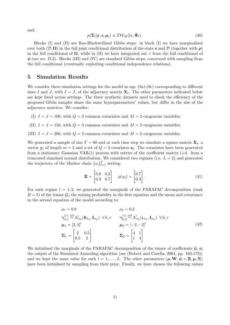
Xi1,...,in,...,iDvin . (1)

Let XtTt=1 and X ∗t Tt=1 be two sequences of binary and real 3-order tensors of size I×J×K,

respectively. In our multilayer network application, Xt is an adjacency tensor and each of itsfrontal slices, Xk,t, represents the adjacency matrix of k-th layer. See Boccaletti et al. (2014)and Kivela et al. (2014) for an introduction to multilayer networks. Let ytTt=1 be a sequenceof real-valued vectors yt = (yt,1, . . . , yt,M )′ representing a set of relevant economic or financialindicators. Our model consists of two systems of equations whose parameters switch over timeaccording to a hidden Markov chain process.

The first set of equations pertains the model for the temporal network. One of the mostrecurrent features of observed networks is edge sparsity, which in random graph theory is definedto be the case in which the number of edges of a graph grows about linearly with the number ofnodes (see (Diestel, 2012, ch.7)). For a finite graph size, we consider a network to be sparse whenthe fraction of edges over the square of nodes, or total degree density, is below 10%. Moreover,the sparsity pattern of many real networks is not time homogeneous. To describe its dynamics

3

. . . . . .st−1 st st+1

Xt−1 Xt Xt+1

yt−1 yt yt+1

Figure 1: Directed acyclic graph (DAG) of the model in eq. (8a)-(8c). Graycircles represent observable variables and white circles latent variables. Dir-ected arrows indicate the direction of causality.

we assume that the probability of observing an edge in each layer of the network is a mixtureof a Dirac mass at 0 and a Bernoulli distribution, where both the mixing probability and theprobability of success are time-varying. Consequently, each entry xijk,t of the tensor Xt (that is,each edge of the corresponding network) is distributed as a zero-inflated logit:

xijk,t|ρ(t),gijk(t) ∼ ρ(t)δ0(xijk,t) + (1− ρ(t))Bern(

xijk,t

∣∣∣∣∣

expz′ijk,tgijk(t)1 + expz′ijk,tgijk(t)

)

. (2)

Notice that this model admits an alternative representation as:

xijk,t|ρ(t),gijk(t) ∼ ρ(t)δ0(xijk,t) + (1− ρ(t))δdijk,t(xijk,t) (3)

dijk,t = 1R+(x∗ijk,t) (4)

x∗ijk,t = z′ijk,tgijk(t) + εijk,t εijk,tiid∼ Logistic(0, 1) . (5)

where zijk,t ∈ RQ is a vector of edge-specific covariates and gijk(t) ∈ R

Q is a time-varying edge-specific vector of parameters. This specification allows to classify the zeros (i.e. absence of edge)into “structural” and “random”, conditionally on arising from the atomic mass, or due to therandomness described in eqs. (4)-(5), respectively. The parameter ρ(t) is thus the time-varyingprobability of observing a structural zero. In the following, without loss of generality, we focuson the case of common set of covariates, that is zijk,t = zt, for t = 1, . . . , T .

The second set of equations regards the vector of economic variables and is given by:

ym,t = µm,t +m,t m,t ∼ N (0, σ2m,t) , (6)

form = 1, . . . ,M and t = 1, . . . , T . In vector form, we denote the mean vector and the covariancematrix by µ(t) and Σ(t), respectively.

The specification of the model is completed with the assumption that the time variationof the parameters µ(t), Σ(t), ρ(t), gijk(t) are driven by a hidden homogeneous Markov chainstTt=1 with discrete, finite state space 1, . . . , L, that is µ(t) = µst , Σ(t) = Σst, ρ(t) = ρstand gijk(t) = gijk,st. The transition matrix of the chain stt is assumed to be time-invariantand denoted by Ξ = (ξ1, . . . , ξL)

′, where each ξl = (ξl,1, . . . , ξl,L)′ is a probability vector and

the transition probability from state i to state j is P(st = j|st−1 = i) = ξi,j, i, j = 1, . . . , L.The causal structure of the model is given in Fig. 1, whereas the description of the systems

follows.In order to give a compact representation of the general model, define Xd = X ∈ R

i1×...×idthe set of real-valued d-order tensors of size (i1 × . . . × id) and X

d0,1 = X∈

Ri1×...×id : Xi1,...,id ∈

0, 1 ⊂ Xd the set of adjacency tensors of size (i1 × . . .× id). Define a linear operator between

4

these two sets by Ψ : Xd → Xd0,1 such that X ∗ 7→ Ψ(X ∗) ∈ 0, 1i1×...×id . Denote the indicator

function for the set A by 1A(x), which takes value 1 if x ∈ A and 0 otherwise, and let R+ be thepositive real half-line. For a matrix X∗

k,t ∈ X I,J it is possible to write the first equation of themodel in matrix form by Ψ(X∗

k,t) = (1R+(x∗ijk,t))i,j , for each slice k of X ∗

t . Eq. (5) postulatesthat each edge xijk admits an individual set of coefficients gijk(t). By collecting all these vectorsalong the indices i, j, k, we can rewrite eq. (5) in compact form by means of a fourth-order tensorG(t) ∈ R

I×J×K×Q, thus obtaining:

X ∗t = G(t) ×4 zt + Et , (7)

where Et ∈ RI×J×K is a third-order tensor with entries εijk,t ∼ Logistic(0, 1) and ×n stands for

the mode-n product between a tensor and a vector previously introduced.The statistical framework we propose for a time series Xt,ytTt=1 is given by the following

system of equations:

Xt = B(t)⊙Ψ(X ∗t ) bijk(t)

iid∼ Bern(1− ρ(t)) (8a)

X ∗t = G(t)×4 zt + Et (8b)

yt = µ(t) +t tiid∼ NM (0,Σ(t)) (8c)

where B(t) is a tensor of the same size of Xt whose entries are independent and identicallydistributed (iid) Bernoulli random variables with probability of success 1 − ρ(t) and ⊙ standsfor the element-by-element Hadamard product (see (Magnus and Neudecker, 1999, ch.3)).

This model can be represented as a SUR (see Zellner (1962)) and also admits an interpreta-tion as a factor model. To this aim, let⊗ denote the Kronecker product (see (Magnus and Neudecker,1999, ch.3)) and define zt = (1, zt)

′, where zt denotes the covariates and Σ1/2 is a mat-rix satisfying Σ1/2Σ1/2 = Σ. In addition, let utt be a martingale difference process andξt = (11(st), . . . ,1L(st))

′. Then we obtain:

Xt = B(t)⊙Ψ(X ∗t ) bijk(t)

iid∼ Bern(1− ρ(t))

X ∗t = G ×4 (ξt ⊗ zt)

′ + Et = G ×4 (ξt, ξt ⊗ zt)′ + Et εijk,t

iid∼ Logistic(0, 1)

yt = (ξt ⊗ µ) + (ξt ⊗Σ1/2)∗t ∗

tiid∼ NM (0M , IM )

ξt+1 = Ξξt + ut E[ut|ut−1] = 0

(9)

3 Bayesian Inference

To derive the likelihood function of the model in eqs. (8a) to (8c) and develop an efficientinferential process, it is useful to start from eq. (2), which describes the statistical model forthe likelihood of each edge as a a zero-inflated logit model. Starting from the seminal workof Lambert (1992), who proposed a modelling framework for count data with a great proportionof zeros, zero-inflated models have been applied to settings where the response variable is notinteger-valued. Binary responses have been considered by Harris and Zhao (2007), who dealtwith an ordered probit model. This is the closest approach to ours, though the specificationin eq. (2) substantially differs in two aspects. First, we use of a logistic link function, whichis known to have slightly fatter tails than the cumulative normal distribution used in probitmodels. Second, differently from the majority of the literature which assumes a constant mixingprobability, the parameter ρ(t) is evolving according to a latent process.

From eq. (2) we derive the probability of observing or not an edge, respectively, as:

P(xijk,t = 1|ρ(t),gijk(t)) = (1− ρ(t))expz′tgijk(t)

1 + expz′tgijk(t)(10a)

5

P(xijk,t = 0|ρ(t),gijk(t)) = ρ(t) + (1− ρ(t))

(

1− expz′tgijk(t)1 + expz′tgijk(t)

)

. (10b)

This allows us to exploit different types of tensor representations (see Kolda and Bader (2009)for a review), in particular for the sake of parsimony, we assume a PARAFAC decompositionwith rank R (assumed fixed and known) for the tensor G(t):

G(t) =R∑

r=1

γ(r)1 (t) γ(r)

2 (t) γ(r)3 (t) γ(r)

4 (t) , (11)

where for each value of the state st the vectors γ(r)h (t) = γ

(r)h,st

, h ∈ 1, 2, 3, 4, r = 1, . . . , R, arethe marginals of the PARAFAC decomposition and have length I, J , K and Q, respectively.By the same argument, we denote G(t) = Gst and gijk(t) = gijk,st. This specification permitsus to achieve two distinct but fundamental goals: (i) parsimony of the model, since for eachvalue of the state st the dimension of the parametric space is reduced from IJKQ to R(I + J +K +Q) parameters; (ii) sparsity of the tensor coefficient, through a suitable choice of the priordistribution for the marginals.

We are given a sample Xt,ytTt=1 and adopt the notation: X = XtTt=1, y = ytTt=1,s = stTt=0, D = DtTt=1 and Ω = ΩtTt=1. Define Tl = t : st = l and Tl = #Tl, for eachregime l = 1, 2. Then, in order to write down the analytic form of the complete data likelihood,we introduce the latent variables stTt=1, taking values st = l, l ∈ 1, 2 and evolving accordingto a discrete Markov chain with transition matrix Ξ ∈ R

L×L. Finally, denote the whole set ofparameters by θ.

The inference is carried out following the Bayesian paradigm and exploiting a data aug-mentation strategy (Tanner and Wong (1987)). The Polya-Gamma scheme for models withbinomial likelihood proposed by Polson et al. (2013) has been proven to outperform existingschemes for Bayesian inference in logistic regression models in terms of computational speedand higher effective sample size. Furthermore, given a normal prior of the vector of parameters,a Polya-Gamma prior on latent variables leads to a conjugate posteriors: the full conditionalfor the parameter vector is normal while that of the latent variable follows a Polya-Gamma.This allows to use a Gibbs sampler instead of a Metropolis-Hastings algorithm, thus avoid-ing the need to choose and adequately tune the proposal distribution. Among recent uses ofthis data augmentation scheme, Wang et al. (2017) used it in a similar framework for network-response regression model, while Holsclaw et al. (2017) exploited it in a time-inhomogeneoushidden Markov model.

The complete data likelihood for X is given by:

L(X ,y,D,Ω, s|θ) =

=

L∏

l=1

∏

t∈Tl

I∏

i=1

J∏

j=1

K∏

k=1

ρdijk,tl · δ0(xijk,t)dijk,t ·

(1− ρl

2

)1−dijk,t

· exp

−ωijk,t

2(z′tgijk,l)

2 + κijk,t(z′tgijk,l)

·L∏

l=1

∏

t∈Tl

(2π)−m/2 |Σl|−1/2 exp

−1

2(yt − µl)

′Σ−1l (yt − µl)

·

T∏

t=1

I∏

i=1

J∏

j=1

K∏

k=1

p(ωijk,t)

·

L∏

g=1

L∏

l=1

ξNgl(s)g,l

· p(s0|Ξ) , (12)

where dij,t is a latent allocation variable and ωij,t is a Polya-Gamma latent variable. See Ap-pendix C for the details of the data augmentation strategy and the derivation of the completedata likelihood.

6

A well known identification issue for mixture models is the label switching problem (see, forexample, Celeux (1998)), which stems from the fact that the likelihood function is invariant torelabelling of the mixture components. This may represent a problem for Bayesian inference,especially when the unobserved components are not well separated, since the associated labelsmay wrongly change across iterations. Several proposals have been made for solving this identi-fication issue (see Fruhwirth-Schnatter (2006) for a review). The permutation sampler proposedby Fruhwirth-Schnatter (2001) can be applied under the assumption of exchangeability of theposterior distribution, which is satisfied when the prior distribution for the transition probab-ilities of the hidden Markov chain is symmetric. Alternatively, there are situations when theparticular application provides meaningful restrictions on the value of some parameters. Theserestrictions generally stem from theoretical results, or interpretation of the different regimes,which is the reason why they are widely used in macroeconomics and finance.

Following this second approach, we can use as identification constraint for the regimes themixing probability of the zero-inflated logit in eq. (3). This can be interpreted as the likelihoodof a “structural” absent edge, therefore by sorting the regimes in decreasing order, from “sparse”to “dense”, we impose: ρ1 > ρ2 > . . . > ρL.

As regards the prior distributions for the parameters of interest, we choose the followingspecifications. Denote ιn the n-dimensional vector of ones. We assume an independent prior on

γ(r)h,l for each regime l = 1, . . . , L, thus representing the a priori ignorance of the different value

of these parameters for varying l. In particular, for each r = 1, . . . , R, each h = 1, . . . , 4 andeach l = 1, . . . , L we specify the global-local shrinkage prior:

π(γ(r)h,l |ζ

rh,l, τ, φr, wh,r,l) ∼ Nnh

(ζrh,l, τφrwh,r,lInh

) (13)

where n = (I, J,Q)′ is a vector containing the length of each vector γ(r)h,l and the prior mean is

set to ζrh,l = 0 for each h = 1, . . . , 4, l = 1, . . . , L, r = 1, . . . , R. The parameter τ represents

the global component of the variance, common to all marginals, φr is level component (specificfor each r = 1, . . . , R) and wh,r is the local component. The choice of a global-local shrinkageprior, as opposed to a spike-and-slab distribution, is motivated by the reduced computationalcomplexity and the capacity to handle high-dimesnional settings.

In addition, for allowing greater flexibility, we assume the following hyper-priors for thevariance components1:

π(τ) ∼ Ga(aτ , bτ ) (14)

π(φ) ∼ Dir(α) α = αιR (15)

π(wh,r,l|λl) ∼ Exp(λ2l /2) ∀h, r, l (16)

π(λl) ∼ Ga(aλl , bλl ) ∀ l . (17)

The further level of hierarchy for the local components wh,r,l is added with the aim offavouring information sharing across local components of the variance (indices h, r) within agiven regime l. This hierarchical prior induces the following marginal prior on the vector wl =(w1,1,l, . . . , w4,R,l)

′:

π(wl) =

∫

R+

R∏

r=1

4∏

h=1

π(wh,r,l|λl)π(λl) dλl

1We use the shape-rate formulation for the gamma distribution, that is for α > 0, β > 0:

x ∼ Ga(α, β) ⇐⇒ f(x) =βα

Γ(α)xα−1

e−βx

x ∈ (0,+∞) .

7

=

∫

R+

(bλl )

aλl

2Γ(aλl )λaλl+8R−1

l exp

−bλl λl −

R∑

r=1

4∑

h=1

wh,r,l

λ2l2

dλl . (18)

The marginal prior for a generic entry wh,r,l is a compound gamma distribution2, that is

p(wh,r,l) ∼ CoGa(1, aλl , 1, bλl ), with aλl > −1. In the univariate case (i.e H = 1, R = 1 and

L = 1), we obtain a generalized Pareto distribution3 π(w) = gP (0, aλ, bλ/aλ).The specification of an exponential distribution for the local component of the variance of the

γ(r)h,l yields a Laplace distribution for each component of the vectors once the wh,r,l is integrated

out, that is γ(r)h,l,i|λl, τ, φr ∼ Laplace(0, λl/

√τφr) for all i = 1, . . . , nh. The marginal distribution

of each entry, integrating all remaining random components, is instead a generalized Paretodistribution.

In probit and logit models it is not possible to identify the coefficients of the latent regressionequation as well as the variance of the noise (e.g., see Wooldridge (2010)). As a consequence,we make the usual identifying restriction by imposing unitary variance for each ǫijk,t.

The mixing probability of the observation model is assumed beta distributed:

π(ρl) ∼ Be(aρl , bρl ) ∀ l = 1, . . . , L . (22)

Concerning the parameters of the second equation (vector yt ∈ Rm), we assume the priors:

π(µl) ∼ NM(µl,Υl) ∀ l = 1, . . . , L (23)

π(Σl) ∼ IWM (νl,Ψl) ∀ l = 1, . . . , L . (24)

Finally, each row of the transition matrix of the Markov chain process st is assumed to be apriori distributed according to a Dirichlet distribution:

π(ξl,:) ∼ Dir(cl,:) ∀ l = 1, . . . , L . (25)

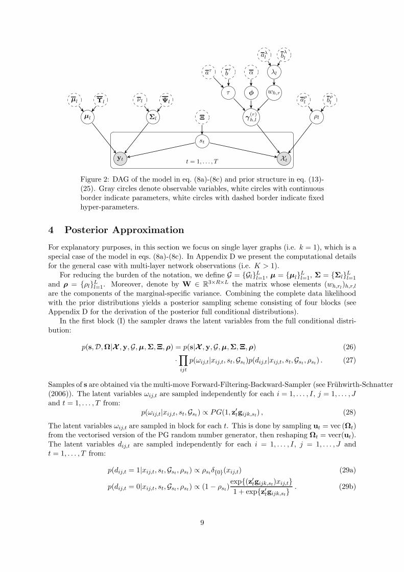
The overall structure of the hierarchical prior distribution is represented graphically by meansof the directed acyclic graph (DAG) in Fig. 2.

2Alternatively, following (Johnson et al., 1995, p.248), this is called generalized beta prime distribution orgeneralized beta distribution of the second kind Be2(α, β, p, q), whose probability density function (with B(α, β)being the usual beta function) is given by:

p(x|α,β, p, q) =1

qB(α, β)p

(

x

q

)αp−1[

1 +

(

x

q

)p]−(α+β)

x ∈ R+, α, β, p, q ∈ R+ . (19)

In our case, the probability density function is defined by a mixture of two gamma distributions (see also Dubey(1970)):

p(x|α,β, 1, q) =

∫ ∞

0

Ga(x|α, p)Ga(p|β, q) dp =qβxα−1(q + x)α+β

B(α, β)x ∈ R+, α, β, q ∈ R+ . (20)

In our case, the parametrisation is (1, aλ, 1, bλ). This special case is also called a Lomax(a, b) distribution withparameters (aλ, bλ).

3The probability density function of the generalized Pareto distribution is:

p(x|µ, ξ, σ) =1

σ

(

1 +(x− µ)

ξσ

)−(ξ+1)

x ∈ R+, µ, ξ ∈ R, σ ∈ R+ . (21)

8

aλl bλ

l

λlα

wh,rφ

bτ

aτ

τ

γ(r)h,l

aρl bρ

l

ρl

Xt

µl Υl

µl

νl Ψl

Σl

yt

Ξ

st

t = 1, . . . , T

Figure 2: DAG of the model in eq. (8a)-(8c) and prior structure in eq. (13)-(25). Gray circles denote observable variables, white circles with continuousborder indicate parameters, white circles with dashed border indicate fixedhyper-parameters.

4 Posterior Approximation

For explanatory purposes, in this section we focus on single layer graphs (i.e. k = 1), which is aspecial case of the model in eqs. (8a)-(8c). In Appendix D we present the computational detailsfor the general case with multi-layer network observations (i.e. K > 1).

For reducing the burden of the notation, we define G = GlLl=1, µ = µlLl=1, Σ = ΣlLl=1

and ρ = ρlLl=1. Moreover, denote by W ∈ R3×R×L the matrix whose elements (wh,rl)h,r,l

are the components of the marginal-specific variance. Combining the complete data likelihoodwith the prior distributions yields a posterior sampling scheme consisting of four blocks (seeAppendix D for the derivation of the posterior full conditional distributions).

In the first block (I) the sampler draws the latent variables from the full conditional distri-bution:

p(s,D,Ω|X ,y,G,µ,Σ,Ξ,ρ) = p(s|X ,y,G,µ,Σ,Ξ,ρ) (26)

·∏

ijt

p(ωij,t|xij,t, st,Gst)p(dij,t|xij,t, st,Gst , ρst) . (27)

Samples of s are obtained via the multi-move Forward-Filtering-Backward-Sampler (see Fruhwirth-Schnatter(2006)). The latent variables ωij,t are sampled independently for each i = 1, . . . , I, j = 1, . . . , Jand t = 1, . . . , T from:

p(ωij,t|xij,t, st,Gst) ∝ PG(1, z′tgijk,st) , (28)

The latent variables ωij,t are sampled in block for each t. This is done by sampling ut = vec (Ωt)from the vectorised version of the PG random number generator, then reshaping Ωt = vecr(ut).The latent variables dij,t are sampled independently for each i = 1, . . . , I, j = 1, . . . , J andt = 1, . . . , T from:

p(dij,t = 1|xij,t, st,Gst , ρst) ∝ ρstδ0(xij,t) (29a)

p(dij,t = 0|xij,t, st,Gst , ρst) ∝ (1− ρst)exp(z′tgijk,st)xij,t1 + expz′tgijk,st

. (29b)

9

Block (II) regards the hyper-parameters which control the variance of the PARAFAC mar-ginals, and have full conditional distribution:

p(τ,φ,W|γ(r)h,lh,l,r) = p(φ|γ(r)

h,lh,l,r,W)p(τ |γ(r)h,lh,l,r,W,φ)p(W|γ(r)

h,lh,l,r,φ, τ) . (30)

The auxiliary variables ψr are sampled independently for r = 1, . . . , R from:

p(ψr|γ(r)h,1h,l,wr) ∝ GiG

2bτ,

3∑

h=1

L∑

l=1

γ(r)′

h,l γ(r)h,l

wh,r, α− n

(31)

then, for each r = 1, . . . , R define:

φr =ψr

∑Rv=1 ψv

. (32)

The parameters φ are sampled in a separate block since they all enter the full conditionals of

wh,r,l and γ(r)h,l . The global variance parameter τ is drawn from:

p(τ |γ(r)h,lh,l,r,W,φ) ∝ GiG

2bτ,

R∑

r=1

3∑

h=1

L∑

l=1

γ(r)′

h,l γ(r)h,l

φrwh,r, (α − n)R

. (33)

The local variance parameters wh,r,l are independently drawn for each h = 1, 2, 3, r = 1, . . . , Rand l = 1, . . . , L from:

p(wh,r,l|γ(r)h,l , φr, τ, λl) ∝ GiG

λ2l ,γ(r)′

h,l γ(r)h,l

τφr, 1− nh

2

. (34)

Finally, denoting wl the collection of all wh,r,l for a given l, the parameters λl are independentlydrawn for each l = 1, . . . , L from:

p(λl|wl) ∝ λaλl+6R−1

l · exp

−λlbλl

·

−λ

2l

2

R∑

r=1

3∑

h=1

wh,r,l

. (35)

The third block (III) concerns the marginals of the PARAFAC decomposition for the tensors

Gl for every l = 1, . . . , L. The vectors γ(r)h,l are sampled independently for all h = 1, 2, 3 and

every r = 1, . . . , R from:

p(γ(r)h,l |X ,W,φ, τ, s,D,Ω) ∝ Nnh

(

ζrh,l, Λ

rh,l

)

. (36)

Finally, in block (IV) are drawn the mixing probability, the transition matrix and the mainparameters of the second equation. The mixing probability is sampled for every l = 1, . . . , Lfrom:

p(ρl|D, s) ∝ Be(al, bl) . (37)

Each row of the transition matrix is independently drawn for every l = 1, . . . , L from:

p(ξl,:) ∝ Dir(c) . (38)

The mean and covariance matrix of the second equation are sampled independently for everyl = 1, . . . , L, respectively from:

p(µl|y, s,Σl) ∝ NM(µl, Υl) (39)

10

and:p(Σl|y, s,µl) ∝ IWM (νl, Ψl) . (40)

Blocks (I) and (II) are Rao-Blackwellized Gibbs steps: in block (I) we have marginalisedover both (D,Ω) in the full joint conditional distribution of the state s and D (together with ρ)in the full conditional of Ω, while in (II) we have integrated out τ from the full conditional ofφ (see sec. D.2). Blocks (III) and (IV) are standard Gibbs steps, concerned with sampling fromthe full conditional (eventually exploiting conditional independence relations).

5 Simulation Results

We consider three simulation settings for the model in eqs. (8a)-(8c) corresponding to differentsizes I and J , with I = J , of the adjacency matrix Xt. The other parameters indicated beloware kept fixed across settings. The three synthetic datasets used to check the efficiency of theproposed Gibbs sampler share the same hyperparameters’ values, but differ in the size of theadjacency matrices. We consider:

(I) I = J = 100, with Q = 3 common covariates and M = 2 exogenous variables;

(II) I = J = 150, with Q = 3 common covariates and M = 2 exogenous variables;

(III) I = J = 200, with Q = 3 common covariates and M = 2 exogenous variables.

We generated a sample of size T = 60 and at each time step we simulate a square matrix Xt, avector yt of length m = 2 and a set of Q = 3 covariates zt. The covariates have been generatedfrom a stationary Gaussian VAR(1) process with entries of the coefficient matrix i.i.d. from atruncated standard normal distribution. We considered two regimes (i.e. L = 2) and generatedthe trajectory of the Markov chain stTt=1 setting:

Ξ =

[

0.8 0.20.3 0.7

]

p(s0) =

[

0.70.3

]

. (41)

For each regime l = 1, 2, we generated the marginals of the PARAFAC decomposition (rankR = 5) of the tensor Gl, the mixing probability in the first equation and the mean and covariancein the second equation of the model according to:

ρ1 = 0.8 ρ2 = 0.2

γ(r)h,1

iid∼ Nnh(0nh

, Inh) ∀h, r γ

(r)h,2

iid∼ Nnh(ιnh

, Inh) ∀h, r

µ1 = [2, 2]′ µ2 = [−2,−2]′

Σ1 =

[

2 0.50.5 2

]

Σ2 =

[

4 11 4

]

(42)

We initialised the marginals of the PARAFAC decomposition of the tensor of coefficients Gl atthe output of the Simulated Annealing algorithm (see (Robert and Casella, 2004, pp. 163-173))and we kept the same value for each l = 1, . . . , L. The other parameters (ρ,W,φ, τ,Ξ,µ,Σ)have been initialised by sampling from their prior. Finally, we have chosen the following values

11

for the hyperparameters:

α = 0.5 bτ = 2 λ = 4 ζrh,l = 0nh∀h, l, r

a1 = 5 b1 = 2 a2 = 2 b2 = 5

µ1 = 0m µ2 = 0m Υ1 = Im Υ2 = Im

ν1 = m ν2 = m Ψ1 = Im Ψ2 = Im

c1 = [8, 4] c2 = [4, 8]

(43)

For each simulation setting, we evaluate the mean square error of the estimated coefficienttensor:

MSE =1

2(MSE1 +MSE2) =

1

2IJK

(∥∥∥G∗

1 − G1

∥∥∥

2

2+∥∥∥G∗

2 − G2

∥∥∥

2

2

)

, (44)

where ‖·‖2 is the Frobenious norm for tensors, i.e.:

∥∥∥G∗

ℓ − Gℓ

∥∥∥

2

2=

I∑

i=1

J∑

j=1

K∑

k=1

(g∗ijk,ℓ − gijk,ℓ)2 . (45)

All simulations have been performed using MATLAB r2016b with the aid of the Tensor Toolboxv.2.64.

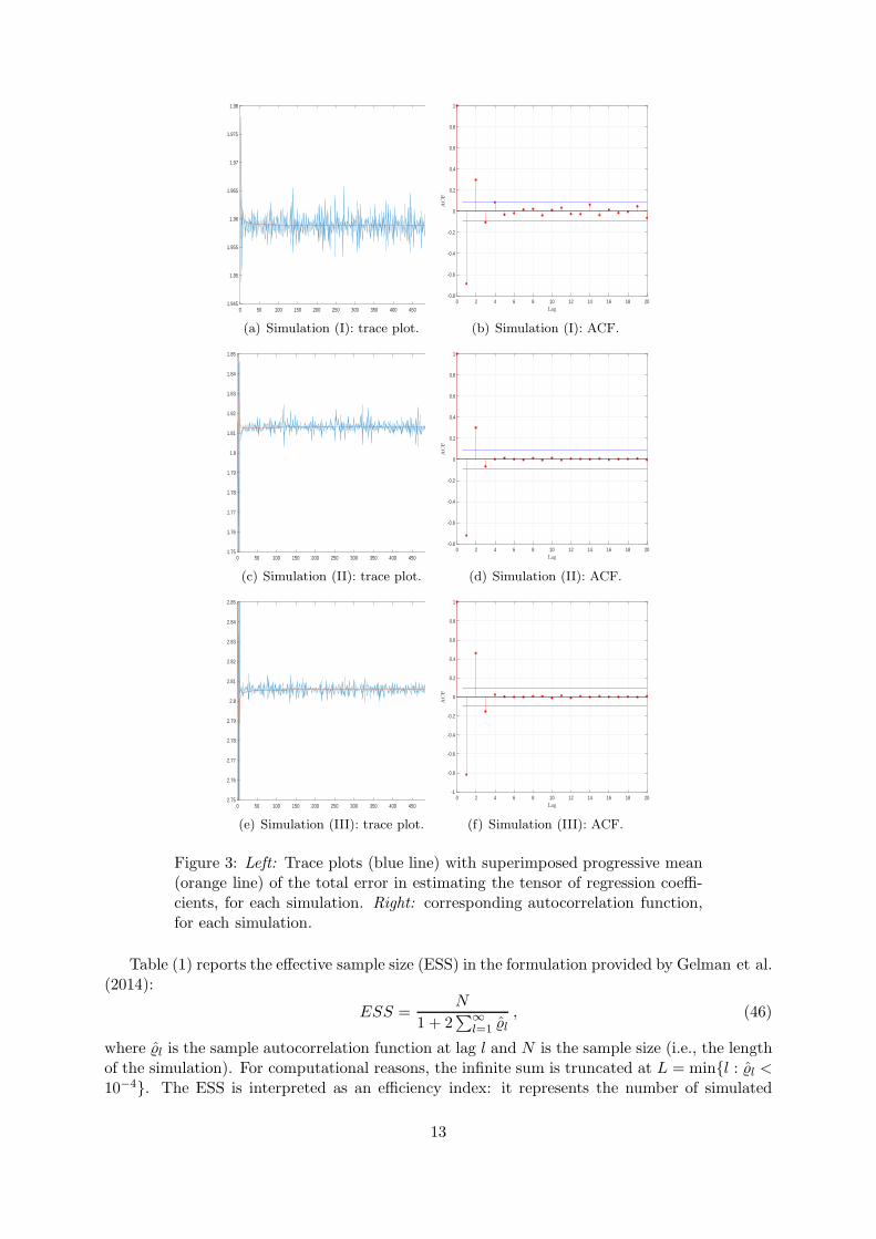
Figs. 3(a)-3(c)-3(e) report the trace plots of the error, for each of the three simulations,respectively, while Figs. 3(b)-3(d)-3(f) plot the corresponding autocorrelation functions. Allthese graphs show that the estimated total error series rapidly stabilises around a small value,meaning that the sampler is able to recover the true value of the tensor parameter. Furthermore,from the analysis of Figs. 3(b)-3(d)-3(f) we can say that the autocorrelation of the posteriordraws of the total error vanishes after three lags, thus representing a first indicator of theefficiency of the sampler. We remind to Appendix F for further details and plots about theperformance of the sampler in each simulated example.

4Available at: http://www.sandia.gov/~tgkolda/TensorToolbox/index-2.6.html

12

0 50 100 150 200 250 300 350 400 450 5001.945

1.95

1.955

1.96

1.965

1.97

1.975

1.98

(a) Simulation (I): trace plot.

0 2 4 6 8 10 12 14 16 18 20-0.8

-0.6

-0.4

-0.2

0

0.2

0.4

0.6

0.8

1

(b) Simulation (I): ACF.

0 50 100 150 200 250 300 350 400 450 5001.75

1.76

1.77

1.78

1.79

1.8

1.81

1.82

1.83

1.84

1.85

(c) Simulation (II): trace plot.

0 2 4 6 8 10 12 14 16 18 20-0.8

-0.6

-0.4

-0.2

0

0.2

0.4

0.6

0.8

1

(d) Simulation (II): ACF.

0 50 100 150 200 250 300 350 400 450 5002.75

2.76

2.77

2.78

2.79

2.8

2.81

2.82

2.83

2.84

2.85

(e) Simulation (III): trace plot.

0 2 4 6 8 10 12 14 16 18 20-1

-0.8

-0.6

-0.4

-0.2

0

0.2

0.4

0.6

0.8

1

(f) Simulation (III): ACF.

Figure 3: Left: Trace plots (blue line) with superimposed progressive mean(orange line) of the total error in estimating the tensor of regression coeffi-cients, for each simulation. Right: corresponding autocorrelation function,for each simulation.

Table (1) reports the effective sample size (ESS) in the formulation provided by Gelman et al.(2014):

ESS =N

1 + 2∑∞

l=1 ˆl, (46)

where ˆl is the sample autocorrelation function at lag l and N is the sample size (i.e., the lengthof the simulation). For computational reasons, the infinite sum is truncated at L = minl : ˆl <10−4. The ESS is interpreted as an efficiency index: it represents the number of simulated

13

Simulation ESS ACF(1) ACF(5)

I 250 ... ...

II 245 ... ...

III 248 ... ...

Table 1: Convergence diagnostic statistics for the total error, for each sim-ulated case. ESS is rounded to the smallest integer.

draws that can be interpreted as iid draws from the posterior distribution (in fact, in presenceof exact iid sampling schemes we have ESS = N). The results in Tab. (1) show that in all threesimulation settings the effective sample size is about half of the length of the simulation.

6 Applications

6.1 Data description

We apply the proposed methodology to the well known dataset of financial networks of Billio et al.(2012), Ahelegbey et al. (2016b), Ahelegbey et al. (2016b), Bianchi et al. (2016). The datasetconsists of T = 110 monthly binary, directed networks estimated via the Granger causality ap-proach, where the nodes are European financial institutions. Other methods for extracting thenetwork structure from data can be used, as this is not relevant for our econometric framework,which applies to any sequence of binary tensors.

The original dataset is composed by the daily closing price series at a daily frequency from29th December 1995 to 16th January 2013 of all the European financial institutions active anddead in order to cope with survivorship bias. It covers a total of 770 European financial firmswhich are traded in 10 European financial markets (core and peripheral). The pairwise Grangercausalities are estimated on daily returns using a rolling window approach with a length foreach window of 252 observations (approximately 1 year). We obtain a total of 4197 adjacencymatrices during the period from 8th January 1997 to 16th January 2013.

Then, we define a binary adjacency matrix for each month by setting an entry to 1 only if thecorresponding Granger-causality link existed for the whole month (i.e. for each trading day of thecorresponding month), and setting the entry to 0 otherwise. Since the panel is unbalanced dueto entry and exit of financial institutions from the sample over time, we consider a subsample oflength T = 110 months (from December 2003 to January 2013) made of 61 financial institutions.

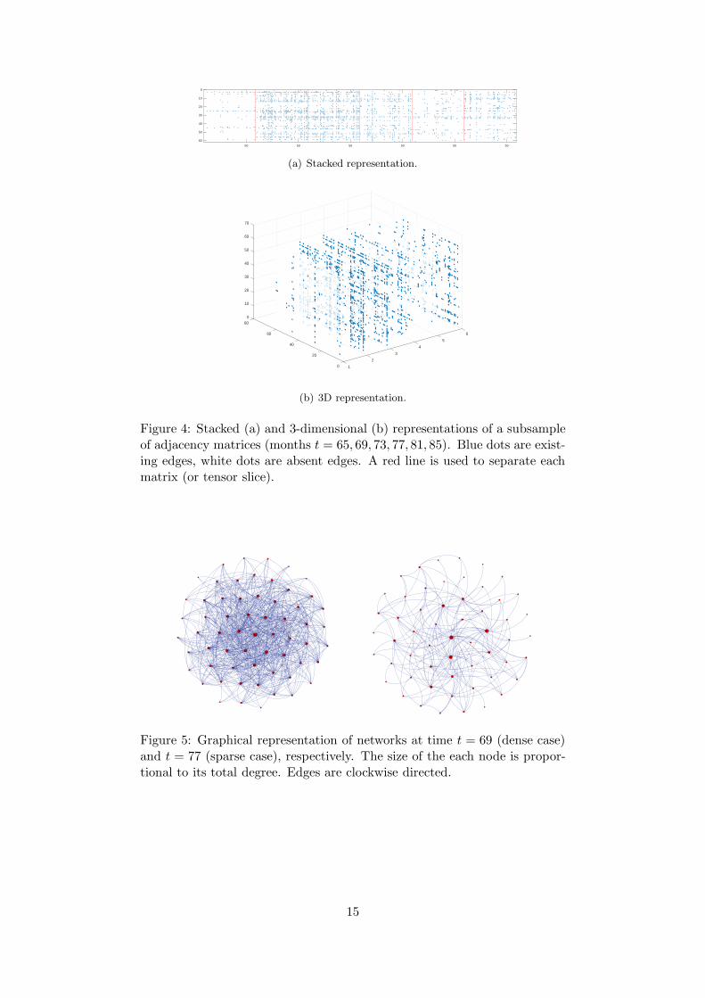
We can visualize a sequence of adjacency matrices representing a time series of networks inseveral ways. Fig. 4(a) shows a stacked representation of a subsample composed by six adjacencymatrices, while Fig. 4(b) plots a 3-dimensional array representation of the same data. In the firstcase, all matrices are stacked horizontally. Instead, the 3-dimensional representation plots eachmatrix in front of the other, as frontal slices of an array. It is possible to interpret the two plotsas equivalent representations of a third-order tensor: in this case, Fig. 4(a) shows the matricisedform (along mode 1) of the tensor, while Fig. 4(b) plots its frontal slices. Finally, Fig. 5 plotsthe graph associated to two of these adjcency matrices. Though this representation allows forvisualising the topology of a network, it is impractical for giving a compact representation ofthe whole time series of networks. Thus, we provide in Fig. 6 the stacked representation of thewhole network sequence. Each row plots twelve time-consecutive adjacency matrices, startingfrom the top-left corner.

The most striking features emerging from Fig. 6 are the time-varying degree distribution andthe temporal clustering of sparse and dense networks.

14

50 50 50 50 50 50

0

10

20

30

40

50

60

(a) Stacked representation.

080

10

20

30

60 6

40

5

50

40

60

4

70

3202

0 1

(b) 3D representation.

Figure 4: Stacked (a) and 3-dimensional (b) representations of a subsampleof adjacency matrices (months t = 65, 69, 73, 77, 81, 85). Blue dots are exist-ing edges, white dots are absent edges. A red line is used to separate eachmatrix (or tensor slice).

2

10

11

13

16

20

37

47

52

60

3

4

5

7

8

9

12

15

17

19

21

23

24

25

26

27

28

29

30

33

34

35

36

39

42

44

45

46

48

50

53

54

55

56

58

59

61

18

49

6

43

1

38

22

14

57

51

40

41

31

32

1

20

3

9

27

37

42

50

51

4

48

5

2

10

13

19

22

23

28

29

44

56

7

41

8

11

12

14

15

16

17

18

38

21

24

25

26

31

32

33

35

47

49

52

55

30

34

36

39

40

43

53

54

45

46

6

Figure 5: Graphical representation of networks at time t = 69 (dense case)and t = 77 (sparse case), respectively. The size of the each node is propor-tional to its total degree. Edges are clockwise directed.

15

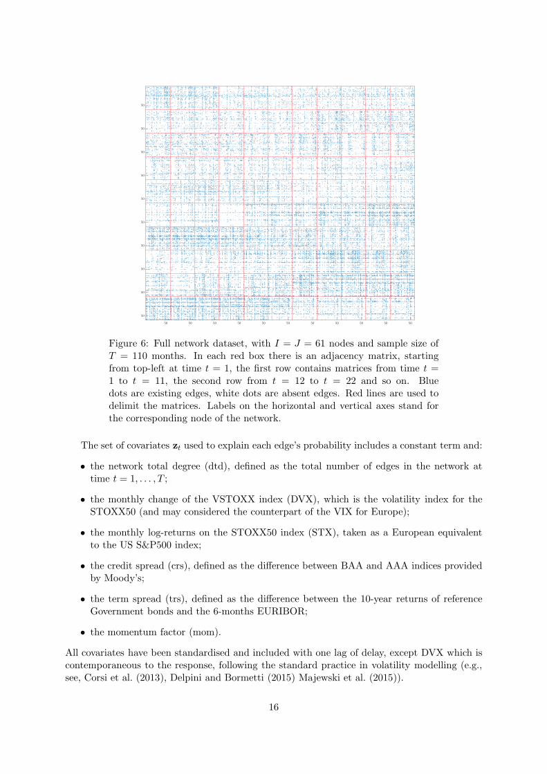
Figure 6: Full network dataset, with I = J = 61 nodes and sample size ofT = 110 months. In each red box there is an adjacency matrix, startingfrom top-left at time t = 1, the first row contains matrices from time t =1 to t = 11, the second row from t = 12 to t = 22 and so on. Bluedots are existing edges, white dots are absent edges. Red lines are used todelimit the matrices. Labels on the horizontal and vertical axes stand forthe corresponding node of the network.

The set of covariates zt used to explain each edge’s probability includes a constant term and:

• the network total degree (dtd), defined as the total number of edges in the network attime t = 1, . . . , T ;

• the monthly change of the VSTOXX index (DVX), which is the volatility index for theSTOXX50 (and may considered the counterpart of the VIX for Europe);

• the monthly log-returns on the STOXX50 index (STX), taken as a European equivalentto the US S&P500 index;

• the credit spread (crs), defined as the difference between BAA and AAA indices providedby Moody’s;

• the term spread (trs), defined as the difference between the 10-year returns of referenceGovernment bonds and the 6-months EURIBOR;

• the momentum factor (mom).

All covariates have been standardised and included with one lag of delay, except DVX which iscontemporaneous to the response, following the standard practice in volatility modelling (e.g.,see, Corsi et al. (2013), Delpini and Bormetti (2015) Majewski et al. (2015)).

16

6.2 Results

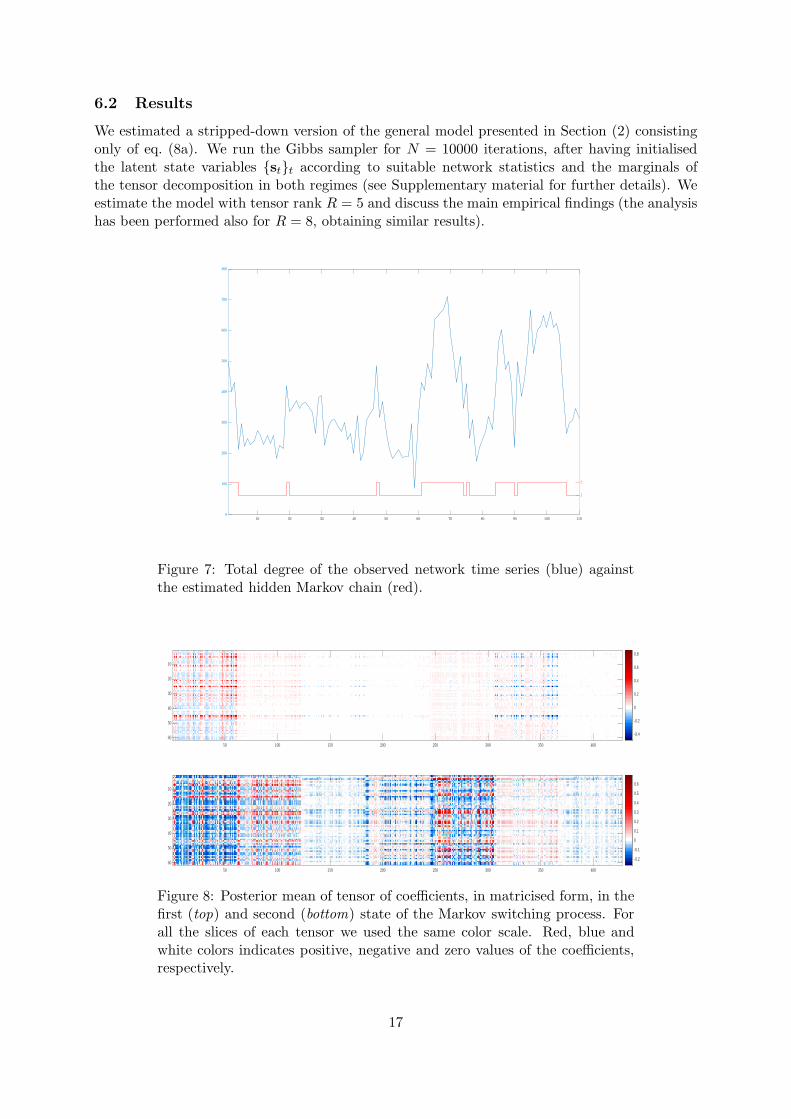
We estimated a stripped-down version of the general model presented in Section (2) consistingonly of eq. (8a). We run the Gibbs sampler for N = 10000 iterations, after having initialisedthe latent state variables stt according to suitable network statistics and the marginals ofthe tensor decomposition in both regimes (see Supplementary material for further details). Weestimate the model with tensor rank R = 5 and discuss the main empirical findings (the analysishas been performed also for R = 8, obtaining similar results).

Figure 7: Total degree of the observed network time series (blue) againstthe estimated hidden Markov chain (red).

-0.4

-0.2

0

0.2

0.4

0.6

0.8

-0.2

-0.1

0

0.1

0.2

0.3

0.4

0.5

0.6

Figure 8: Posterior mean of tensor of coefficients, in matricised form, in thefirst (top) and second (bottom) state of the Markov switching process. Forall the slices of each tensor we used the same color scale. Red, blue andwhite colors indicates positive, negative and zero values of the coefficients,respectively.

17

0

0.2

0.4

0.6

0.8

-0.2

-0.1

0

0.1

0.2

0.3

0.4

-0.02

0

0.02

0.04

0.06

0.08

0.1

0.12

0.14

-0.1

0

0.1

0.2

0.3

0.4

-0.12

-0.1

-0.08

-0.06

-0.04

-0.02

0

-0.1

-0.05

0

0.05

-0.01

0

0.01

0.02

0.03

0.04

-0.2

-0.15

-0.1

-0.05

0

0.05

0.1

-0.06

-0.04

-0.02

0

0.02

0.04

-0.2

-0.1

0

0.1

0.2

0.3

0.4

0.5

0.6

-0.4

-0.3

-0.2

-0.1

0

-0.1

-0.05

0

0.05

0.1

0.15

0.2

-0.02

-0.01

0

0.01

0.02

0.03

-0.1

-0.08

-0.06

-0.04

-0.02

0

0.02

0.04

0.06

Figure 9: Posterior mean of tensor of coefficients, in matricised form, inthe first (top) and second (bottom) state of the Markov switching process.For each slice of each tensor we used a different color scale. Red, blue andwhite colors indicates positive, negative and zero values of the coefficients,respectively.

Figure 10: Posterior distribution (left plot) and MCMC output (right plots)of the quadratic norm of the tensor of coefficients, in regime 1 (blue) andregime 2 (orange).

18

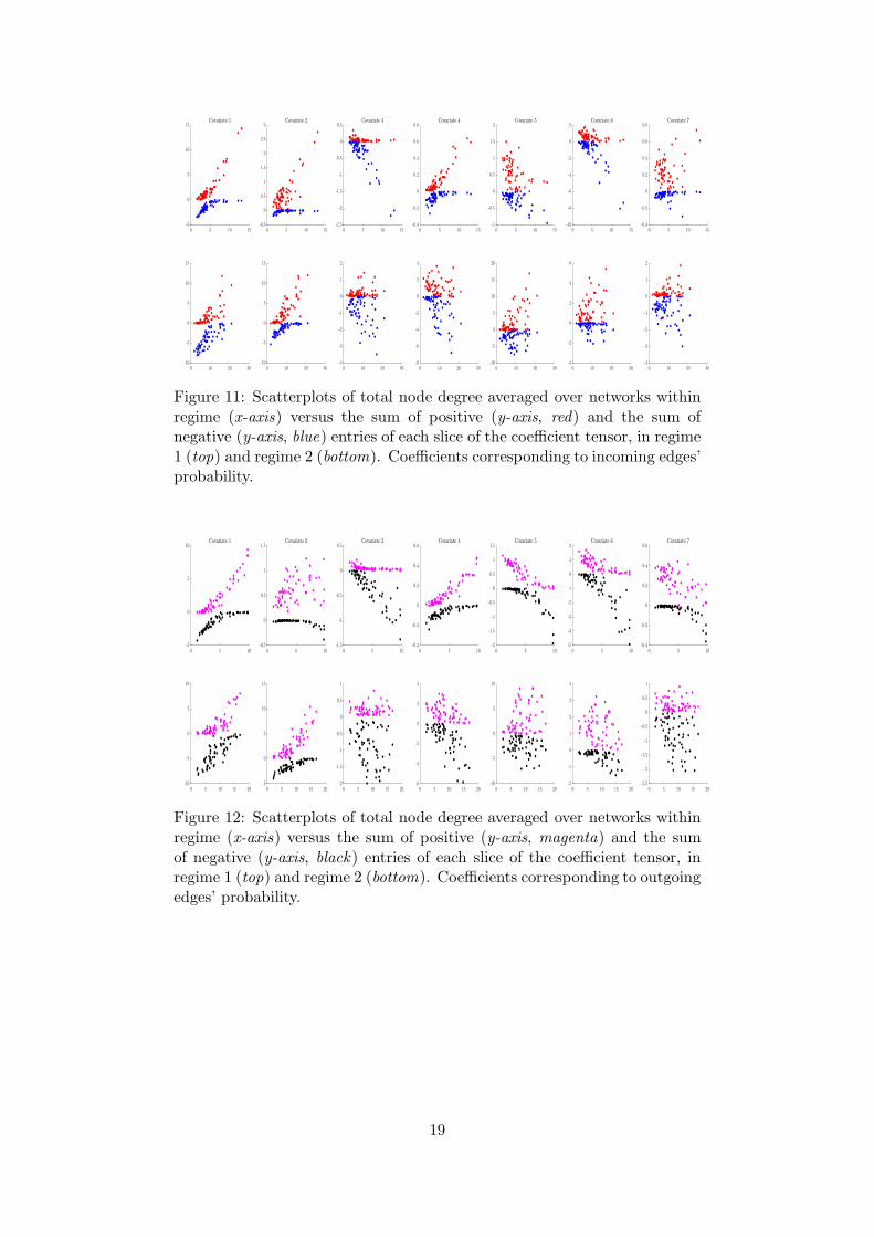
Figure 11: Scatterplots of total node degree averaged over networks withinregime (x-axis) versus the sum of positive (y-axis, red) and the sum ofnegative (y-axis, blue) entries of each slice of the coefficient tensor, in regime1 (top) and regime 2 (bottom). Coefficients corresponding to incoming edges’probability.

Figure 12: Scatterplots of total node degree averaged over networks withinregime (x-axis) versus the sum of positive (y-axis, magenta) and the sumof negative (y-axis, black) entries of each slice of the coefficient tensor, inregime 1 (top) and regime 2 (bottom). Coefficients corresponding to outgoingedges’ probability.

19

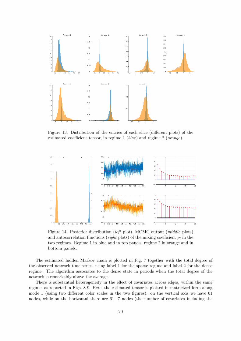
Figure 13: Distribution of the entries of each slice (different plots) of theestimated coefficient tensor, in regime 1 (blue) and regime 2 (orange).

Figure 14: Posterior distribution (left plot), MCMC output (middle plots)and autocorrelation functions (right plots) of the mixing coefficient ρl in thetwo regimes. Regime 1 in blue and in top panels, regime 2 in orange and inbottom panels.

The estimated hidden Markov chain is plotted in Fig. 7 together with the total degree ofthe observed network time series, using label 1 for the sparse regime and label 2 for the denseregime. The algorithm associates to the dense state in periods when the total degree of thenetwork is remarkably above the average.

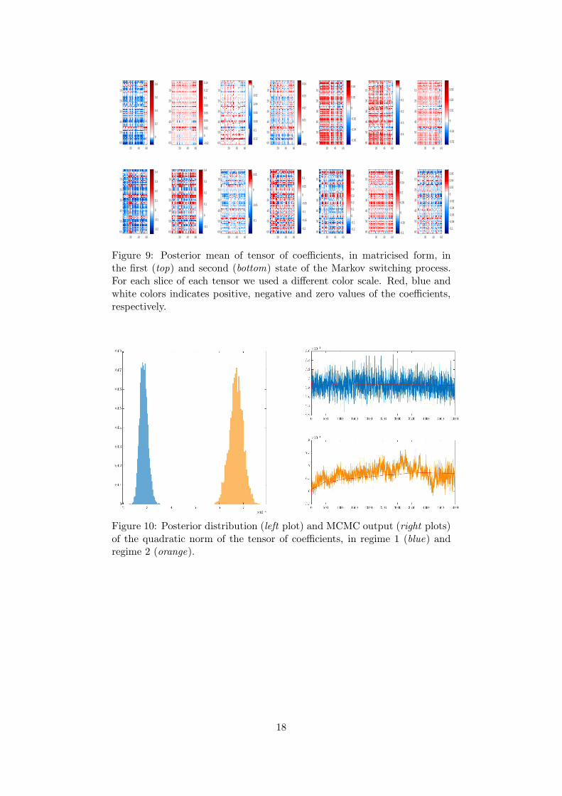
There is substantial heterogeneity in the effect of covariates across edges, within the sameregime, as reported in Figs. 8-9. Here, the estimated tensor is plotted in matricized form alongmode 1 (using two different color scales in the two figures): on the vertical axis we have 61nodes, while on the horizontal there are 61 · 7 nodes (the number of covariates including the

20

constant), corresponding to 7 matrices, one for each covariate, horizontally stacked. The entry(i, j) of matrix in position k reports the coefficient of the k-th covariate on the probability ofobserving the edge (i, j). Thus, within the same regime we observe a significant variation ofboth the sign and the magnitude of the effect of a covariate on the probability of observing anedge. In words, there is not a single covariate able to explain (and predict) an edge’s probabilityby itself, but several indicators are required. Moreover, a model with pooled time series fails tocapture such heterogeneity. The posterior mean is 1.56 in regime 1 and 4.63 in regime 2, but inboth cases it is not significantly different from zero, that is, it lies inside a 95% credible intervalaround zero (see Fig. 43 in Appendix G). This is in contrast with our model, where the fractionof tensor entries statistically different from zero is 12% and 36% in regime 1 and 2, respectively.Thus, we conclude that a pooled model is not suited for describing the heterogeneous effects ofthe various covariates on the different edges, whereas our model is able to capture them.

We find substantial evidence in favour of major changes of the effects that the covariatesexert on the edges’ probability in the two regimes. By comparing the two matricized tensors inFig. 8 we note that both the sign and the magnitude of the coefficients differ in the two states.The interpretation is that, according to the regime, the probability of observing a link betweentwo nodes is driven by a different set of variables but also the qualitative influence (i.e. the signof the coefficient) of the same regressor varies. For example, on average, the credit spread seemsto exert a positive effect on the probability of observing an edge in the sparse regime, while itseffect in the dense regime has higher magnitude and acts in the opposite direction.

Fig. 11 reports, for each regime and covariate, the scatterplot of the total degree of each node(horizontal axis), averaged within regime, against the sum of all negative and positive coefficients’values for the probability of observing an incoming edge. Similarly, Fig. 12 shows the same plotconsidering the effects on the probability of observing an outcoming edge. Together, these plotsallow to detect the existence of a relation between the overall positive and negative magnitudeof the effects of the covariates on the probability of observing an edge, conditionally on the totaldegree of the node to which the link is attached. The results show that for several covariatessuch an association exists: on average, more central nodes (i.e. those with higher total degree)tend to have higher probability of establishing an edge, either incoming or outgoing. This isdue to the upward sloping shape of the scatterplot. It is remarkable to notice that for differentcovariates, such as the momentum factor, there is a different relation for negative and positiveeffects: for increasingly central nodes, both sums tend to more extreme values. Moreover, bycomparing the results in Figs. 11-12 we see that the results are similar if we look either atincoming or outgoing edges. Finally, between regimes there seems to be no change except forthe strength of the relation, which appears stronger in the second one (corresponding to thedense state of the network).

In Fig. 13 we plot the distribution of the entries of each slice (over the edges), for everyregime, for a more qualitative analysis of the change of the coefficients’ values between regimes.There is a different dispersion in the cross-sectional distribution of the coefficients’ estimates.In particular, all distributions appear more concentrated around zero in the sparse state, whilein the dense regime the mean value is different (and varies according to the covariate) and alldistributions show fatter tails than in sparse state.

As a summary statistic, Fig. 10 reports the distribution and the trace plots of the quadraticnorm of the tensor coefficients in each regime. The two distributions are well separated, withthe norm in the first regimes concentrated around smaller values than in the second regime.This implies that, on average, in the sparse state there is a higher probability that the zeros(i.e. absence of edges) are due to the structural component (that is, the Dirac mass in eq. (3)),moreover the probability of success of the Bernoulli distribution is smaller than in the denseregime.

21

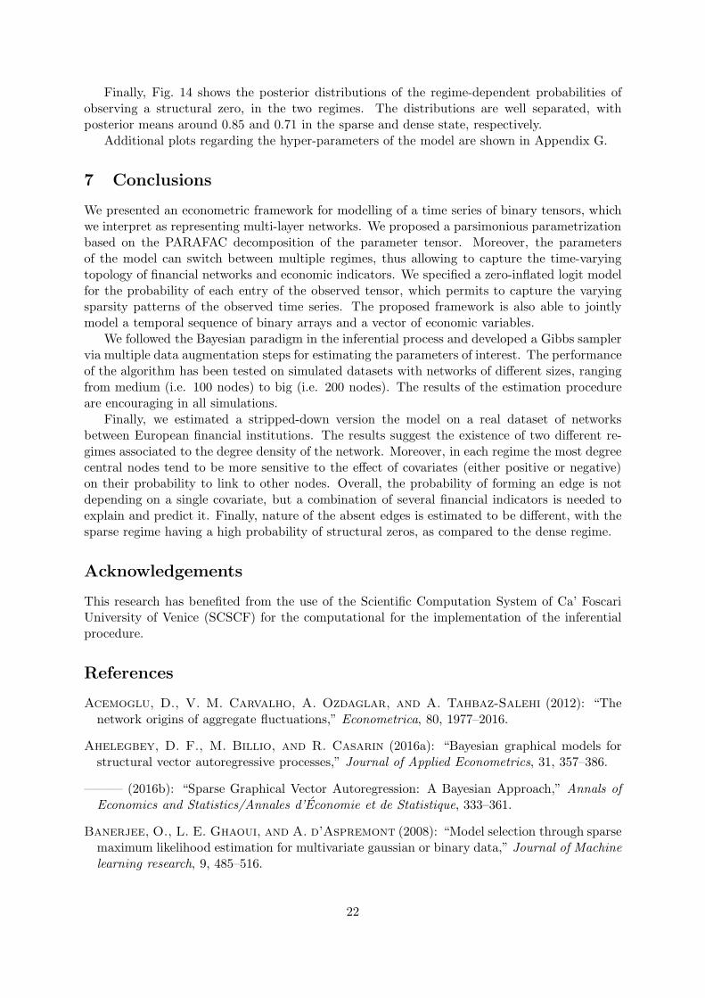
Finally, Fig. 14 shows the posterior distributions of the regime-dependent probabilities ofobserving a structural zero, in the two regimes. The distributions are well separated, withposterior means around 0.85 and 0.71 in the sparse and dense state, respectively.

Additional plots regarding the hyper-parameters of the model are shown in Appendix G.

7 Conclusions

We presented an econometric framework for modelling of a time series of binary tensors, whichwe interpret as representing multi-layer networks. We proposed a parsimonious parametrizationbased on the PARAFAC decomposition of the parameter tensor. Moreover, the parametersof the model can switch between multiple regimes, thus allowing to capture the time-varyingtopology of financial networks and economic indicators. We specified a zero-inflated logit modelfor the probability of each entry of the observed tensor, which permits to capture the varyingsparsity patterns of the observed time series. The proposed framework is also able to jointlymodel a temporal sequence of binary arrays and a vector of economic variables.

We followed the Bayesian paradigm in the inferential process and developed a Gibbs samplervia multiple data augmentation steps for estimating the parameters of interest. The performanceof the algorithm has been tested on simulated datasets with networks of different sizes, rangingfrom medium (i.e. 100 nodes) to big (i.e. 200 nodes). The results of the estimation procedureare encouraging in all simulations.

Finally, we estimated a stripped-down version the model on a real dataset of networksbetween European financial institutions. The results suggest the existence of two different re-gimes associated to the degree density of the network. Moreover, in each regime the most degreecentral nodes tend to be more sensitive to the effect of covariates (either positive or negative)on their probability to link to other nodes. Overall, the probability of forming an edge is notdepending on a single covariate, but a combination of several financial indicators is needed toexplain and predict it. Finally, nature of the absent edges is estimated to be different, with thesparse regime having a high probability of structural zeros, as compared to the dense regime.

Acknowledgements

This research has benefited from the use of the Scientific Computation System of Ca’ FoscariUniversity of Venice (SCSCF) for the computational for the implementation of the inferentialprocedure.

References

Acemoglu, D., V. M. Carvalho, A. Ozdaglar, and A. Tahbaz-Salehi (2012): “Thenetwork origins of aggregate fluctuations,” Econometrica, 80, 1977–2016.

Ahelegbey, D. F., M. Billio, and R. Casarin (2016a): “Bayesian graphical models forstructural vector autoregressive processes,” Journal of Applied Econometrics, 31, 357–386.

——— (2016b): “Sparse Graphical Vector Autoregression: A Bayesian Approach,” Annals ofEconomics and Statistics/Annales d’Economie et de Statistique, 333–361.

Banerjee, O., L. E. Ghaoui, and A. d’Aspremont (2008): “Model selection through sparsemaximum likelihood estimation for multivariate gaussian or binary data,” Journal of Machinelearning research, 9, 485–516.

22

Bianchi, D., M. Billio, R. Casarin, and M. Guidolin (2016): “Modeling Sys-temic Risk with Markov Switching Graphical SUR Models,” Available at SSRN: ht-tps://ssrn.com/abstract=2537986.

Billio, M., M. Caporin, R. Panzica, and L. Pelizzon (2015): “Network connectivity andsystematic risk,” Tech. rep., European Financial Management Association.

Billio, M., M. Getmansky, A. W. Lo, and L. Pelizzon (2012): “Econometric measures ofConnectedness and Systemic Risk in the Finance and Insurance Sectors,” Journal of FinancialEconomics, 104, 535–559.

Boccaletti, S., G. Bianconi, R. Criado, C. I. Del Genio, J. Gomez-Gardenes,

M. Romance, I. Sendina-Nadal, Z. Wang, and M. Zanin (2014): “The Structure andDynamics of Multilayer Networks,” Physics Reports, 544, 1–122.

Carroll, J. D. and J.-J. Chang (1970): “Analysis of Individual Differences in multidimen-sional Scaling via an N-way Generalization of “Eckart-Young” Decomposition,” Psychomet-rica, 35, 283–319.

Casarin, R., D. Sartore, and M. Tronzano (2018): “A Bayesian Markov-switching cor-relation model for contagion analysis on exchange rate markets,” Journal of Business & Eco-nomic Statistics, 36, 101–114.

Celeux, G. (1998): “Bayesian inference for mixture: The label switching problem,” inCompstat, Springer, 227–232.

Chaney, T. (2014): “The network structure of international trade,” The American economicreview, 104, 3600–3634.

Chib, S., F. Nardari, and N. Shephard (2002): “Markov Chain Monte Carlo methods forstochastic volatility models,” Journal of Econometrics, 108, 281–316.

Christakis, N. A. and J. H. Fowler (2008): “The collective dynamics of smoking in a largesocial network,” New England journal of medicine, 358, 2249–2258.

Cichocki, A., N. Lee, I. Oseledets, A. Phan, Q. Zhao, and D. Mandic (2016): “Low-Rank Tensor Networks for Dimensionality Reduction and Large-Scale Optimization Problems:Perspectives and Challenges PART 1,” arXiv preprint arXiv:1609.00893.

Cichocki, A., D. Mandic, L. De Lathauwer, G. Zhou, Q. Zhao, C. Caiafa, and H. A.

Phan (2015): “Tensor Decompositions for Signal Processing Applications: From two-way toMultiway Component Analysis,” IEEE Signal Processing Magazine, 32, 145–163.

Cichocki, A., R. Zdunek, A. H. Phan, and S.-i. Amari (2009): Nonnegative matrix andtensor factorizations: applications to exploratory multi-way data analysis and blind sourceseparation, John Wiley & Sons.

Corsi, F., N. Fusari, and D. La Vecchia (2013): “Realizing smiles: Options pricing withrealized volatility,” Journal of Financial Economics, 107, 284–304.

Delpini, D. and G. Bormetti (2015): “Stochastic volatility with heterogeneous time scales,”Quantitative Finance, 15, 1597–1608.

Di Giovanni, J., A. A. Levchenko, and I. Mejean (2014): “Firms, destinations, andaggregate fluctuations,” Econometrica, 82, 1303–1340.

23

Diebold, F. X. and K. Yılmaz (2014): “On the network topology of variance decompositions:Measuring the connectedness of financial firms,” Journal of Econometrics, 182, 119–134.

Diestel, R. (2012): Graph Theory, vol. 173 of Graduate Texts in Mathematics, Springer.

Dubey, S. D. (1970): “Compound gamma, beta and F distributions,” Metrika, 16, 27–31.

Dueker, M. J. (1997): “Markov switching in GARCH processes and mean-reverting stock-market volatility,” Journal of Business & Economic Statistics, 15, 26–34.

——— (2005): “Dynamic forecasts of qualitative variables: a Qual VAR model of US recessions,”Journal of Business & Economic Statistics, 23, 96–104.

Durante, D. and D. B. Dunson (2014): “Bayesian Logistic Gaussian Process Models for Dy-namic Networks,” Proceedings of the 17th International Conference on Artificial Intelligenceand Statistics (AISTATS), 33.

Fruhwirth-Schnatter, S. (2001): “Markov Chain Monte Carlo estimation of classical anddynamic switching and mixture models,” Journal of the American Statistical Association, 96,194–209.

——— (2006): Finite Mixture and Markov Switching Models, Springer.

Gelman, A., J. B. Carlin, H. S. Stern, D. B. Dunson, A. Vehtari, and D. B. Rubin

(2014): Bayesian data analysis, vol. 2, CRC Press.

Graham, B. S. (2017): “An econometric model of network formation with degree heterogen-eity,” Econometrica, 85, 1033–1063.

Guhaniyogi, R., S. Qamar, and D. B. Dunson (2017): “Bayesian Tensor Regression,”Journal of Machine Learning Research, 18, 1–31.

Haas, M., S. Mittnik, and M. S. Paolella (2004): “A new approach to Markov-switchingGARCH models,” Journal of Financial Econometrics, 2, 493–530.

Hackbusch, W. (2012): Tensor Spaces and Numerical Tensor Calculus, Springer Science &Business Media.

Hamilton, J. D. (1989): “A new approach to the economic analysis of nonstationary timeseries and the business cycle,” Econometrica, 57, 357–384.

Hamilton, J. D. and R. Susmel (1994): “Autoregressive conditional heteroskedasticity andchanges in regime,” Journal of Econometrics, 64, 307–333.

Harris, M. N. and X. Zhao (2007): “A zero-inflated ordered probit model, with an applicationto modelling tobacco consumption,” Journal of Econometrics, 141, 1073–1099.

Harshman, R. A. (1970): “Foundations of the PARAFAC Procedure: Models and Conditionsfor an ”Explanatory” Multi-modal Factor Analysis,” UCLA Working Papers in Phonetics,16, 1- 84.

Holsclaw, T., A. M. Greene, A. W. Robertson, and P. Smyth (2017): “Bayesian Non-Homogeneous Markov Models via Polya-Gamma Data Augmentation with Applications toRainfall Modeling,” arXiv preprint arXiv:1701.02856.

24

Johnson, N. L., S. Kotz, and N. Balakrishnan (1995): Continuous univariate distribu-tions, vol. 2 of Wiley series in Probability and Mathematical Statistics: Applied Probabilityand Statistics, Wiley, New York.

Kaufmann, S. (2000): “Measuring business cycles with a dynamic Markov switching factormodel: An assessment using Bayesian simulation methods,” The Econometrics Journal, 3,39–65.

——— (2010): “Dating and forecasting turning points by Bayesian clustering with dynamicstructure: A suggestion with an application to Austrian data,” Journal of Applied Economet-rics, 25, 309–344.

——— (2015): “K-state switching models with time-varying transition distributions—Does loangrowth signal stronger effects of variables on inflation?” Journal of Econometrics, 187, 82–94.

Kiers, H. A. (2000): “Towards a Standardized Notation and Terminology in Multiway Ana-lysis,” Journal of Chameometrics, 14, 105–122.

Kim, C.-J. and C. R. Nelson (1998): “Business cycle turning points, a new coincident index,and tests of duration dependence based on a dynamic factor model with regime switching,”Review of Economics and Statistics, 80, 188–201.

Kivela, M., A. Arenas, M. Barthelemy, J. P. Gleeson, Y. Moreno, and M. A.

Porter (2014): “Multilayer networks,” Journal of Complex Networks, 2, 203–271.

Klaassen, F. (2002): “Improving GARCH volatility forecasts with regime-switching GARCH,”in Advances in Markov-Switching Models, Springer, 223–254.

Koh, K., S.-J. Kim, and S. Boyd (2007): “An interior-point method for large-scale l1-regularized logistic regression,” Journal of Machine learning research, 8, 1519–1555.

Kolda, T. G. and B. W. Bader (2009): “Tensor Decompositions and Applications,” SIAMReview, 51, 455–500.

Kroonenberg, P. M. (2008): Applied multiway data analysis, John Wiley & Sons.

Lambert, D. (1992): “Zero-inflated Poisson regression, with an application to defects in man-ufacturing,” Technometrics, 34, 1–14.

Lee, N. and A. Cichocki (2016): “Fundamental Tensor Operations for Large-Scale DataAnalysis in Tensor Train Formats,” arXiv preprint arXiv:1405.7786.

Magnus, J. R. and H. Neudecker (1999): Matrix Differential Calculus with Applications inStatistics and Econometrics, Wiley, New York.

Majewski, A. A., G. Bormetti, and F. Corsi (2015): “Smile from the past: A generaloption pricing framework with multiple volatility and leverage components,” Journal of Eco-nometrics, 187, 521–531.

Mele, A. (2017): “A structural model of Dense Network Formation,” Econometrica, 85, 825–850.

Neal, R. M. (2011): “MCMC using Hamiltonian dynamics,” in Handbook of Markov ChainMonte Carlo, ed. by S. Brooks, A. Gelman, J. L. Galin, and X.-L. Meng, Chapman & Hall/CRC, chap. 5.

25

Polson, N. G., J. G. Scott, and J. Windle (2013): “Bayesian Inference for Logistic Modelsusing Polya–Gamma Latent Variables,” Journal of the American Statistical Association, 108,1339–1349.

Ravikumar, P., M. J. Wainwright, J. D. Lafferty, et al. (2010): “High-dimensionalIsing model selection using l1-regularized logistic regression,” The Annals of Statistics, 38,1287–1319.

Robert, C. P. and G. Casella (2004): Monte Carlo Statistical Methods, Springer.

Schildcrout, J. S. and P. J. Heagerty (2005): “Regression analysis of longitudinal binarydata with time-dependent environmental covariates: bias and efficiency,” Biostatistics, 6,633–652.

Sherman, M., T. V. Apanasovich, and R. J. Carroll (2006): “On estimation in binaryautologistic spatial models,” Journal of Statistical Computation and Simulation, 76, 167–179.

Sims, C. A., D. F. Waggoner, and T. Zha (2008): “Methods for inference in large multiple-equation Markov-switching models,” Journal of Econometrics, 146, 255–274.

Sims, C. A. and T. Zha (2006): “Were there regime switches in US monetary policy?” TheAmerican Economic Review, 96, 54–81.

Smith, D. R. (2002): “Markov-switching and stochastic volatility diffusion models of short-terminterest rates,” Journal of Business & Economic Statistics, 20, 183–197.

Springer, M. and W. Thompson (1970): “The distribution of products of beta, gamma andGaussian random variables,” SIAM Journal on Applied Mathematics, 18, 721–737.

Taddy, M. (2013): “Multinomial inverse regression for text analysis,” Journal of the AmericanStatistical Association, 108, 755–770.

Taddy, M. A. (2010): “Autoregressive mixture models for dynamic spatial Poisson processes:Application to tracking intensity of violent crime,” Journal of the American Statistical Asso-ciation, 105, 1403–1417.

Tanner, M. A. and W. H. Wong (1987): “The calculation of posterior distributions by dataaugmentation,” Journal of the American Statistical Association, 82, 528–540.

Turney, P. D. (2002): “Thumbs up or thumbs down? Semantic orientation applied to unsu-pervised classification of reviews,” in Proceedings of the 40th annual meeting on associationfor computational linguistics, Association for Computational Linguistics, 417–424.

Van Dyk, D. A. and T. Park (2008): “Partially collapsed Gibbs samplers: Theory andmethods,” Journal of the American Statistical Association, 103, 790–796.

Visaya, M. V., D. Sherwell, B. Sartorius, and F. Cromieres (2015): “Analysis of BinaryMultivariate Longitudinal Data via 2-Dimensional Orbits: An Application to the AgincourtHealth and Socio-Demographic Surveillance System in South Africa,” PloS one, 10, e0123812.

Wang, L., D. Durante, R. E. Jung, and D. B. Dunson (2017): “Bayesian network–response regression,” Bioinformatics, 33, 1859–1866.

Wilbur, J., J. Ghosh, C. Nakatsu, S. Brouder, and R. Doerge (2002): “VariableSelection in High-Dimensional Multivariate Binary Data with Application to the Analysis ofMicrobial Community DNA Fingerprints,” Biometrics, 58, 378–386.

26

Wooldridge, J. M. (2010): Econometric analysis of cross section and panel data, MIT press.

Yue, Y. R., M. A. Lindquist, and J. M. Loh (2012): “Meya-analysis of functional neuroima-ging data using Bayesian nonparametric binary regression,” The Annals of Applied Statistics,697–718.

Zellner, A. (1962): “An efficient method of estimating seemingly unrelated regressions andtests for aggregation bias,” Journal of the American Statistical Association, 57, 348–368.

A Tensor calculus and decompositions

In this section we introduce some notation for multilinear arrays (i.e. tensors) and some basic op-erations defined on them: the operations on tensors and between tensors and lower-dimensionalobjects (such as matrices and vectors) and the representation results for tensors (or tensor decom-position/approximation). A noteworthy introduction to tensors and corresponding operationsis in Lee and Cichocki (2016), while a remarkable reference for tensor decomposition methodsis Kolda and Bader (2009). Throughout the paper, we use the following notation: matricesare represented by boldface uppercase letters, vectors by boldface lowercase letters, scalars bylowercase letters and, finally, calligraphic letters denote tensors, if not differently specified.

A multidimensional array is an object which generalises the concept of matrix. It mayhave an arbitrary number of dimensions (or modes), whose number is the order of the tensor.Consequently, a matrix is a second order tensor. By convention, we denote a whole column (orrow) of a matrix by the symbol “:” and the same is used for tensors, where this symbol denotesthat we are considering the corresponding whole dimension. The mode-k fiber of a tensor is ageneralization of the concept of row/column in the matrix case: it is the vector obtained alongthe dimension k by fixing all the other dimensions. Differently from the bi-dimensional case,however, with higher order arrays it is possible to identify also slices (i.e. bi-dimensional fibersof matrices) or generalizations of them, by fixing all but two or more dimensions (or modes) ofthe tensor. For example, the mode-k fiber of the tensor X is denoted by:

X(i1,...,ik−1,:,:,ik+2,...,iD) ∀ k ∈ 1, . . . ,D . (A.1)

The operation of transforming a D-array X into a matrix is called matricization. The mode-nmatricization, denoted by X(n), consists in re-arranging all the mode-n fibers to be the columns

of a matrix, which will have size X(n) ∈ Rdn×d(−n) with d(−n) = Πi 6=ndi. For detailed examples,

see Kolda and Bader (2009). Analogously to the matrix version, the vectorization of a tensorconsists in stacking all the elements in a unique vector of dimension d = Πidi. Notice that, theordering of the elements is not important as long as it is consistent across the calculations.

Many product operations have been defined for tensors, but here we constrain ourselves tothe operator used in this work and we point to Lee and Cichocki (2016) for a summary of otheroperators. The mode−n product between a tensor X and a vector v ∈ R

dn can be interpreted asthe standard Euclidean inner product between the vector and each mode-n fiber of the tensor.Consequently, this operator suppresses one dimension of the tensor and results in a lower ordertensor. It is defined, element-wise, by:

Y(i1,...,in−1,in+1,...,iD) = (X ×n v)(i1,...,in−1,in+1,...,iD) =

dn∑

in

Xi1,...,iDvin , (A.2)

with Y ∈ Rd1×...,dn−i,dn+1,...×dD . Notice that this product is not commutative, since the order of

the elements in the multiplication is relevant.

27

Finally, let Y ∈ RdY1 ×...×dYM and X ∈ R

dX1 ×...×dXN . The outer product of two tensors5 is thetensor Z ∈ R

dY1 ×...×dYM×dX1 ×...×dXN whose entries are:

Zi1,...,iM ,j1,...,jN = (Y X )i1,...,iM ,j1,...,jN = Yi1,...,iMXj1,...,jN . (A.3)

For example, the outer product of two vectors is a matrix, while the outer product of twomatrices is a tensor of order 4. As a special case, the outer product of two column vectors a, bcan be equivalently represented by means of the Kronocker product ⊗:

a b = b⊗ a = a · b′ . (A.4)

We now define two tensor representations, or decompositions, which are useful in two re-spects: (i) the algebraic objects that form the decomposition are generally low dimensional andmore easily tractable than the tensor; (ii) they can be used to provide a good approximation ofthe original array. Also, let us denote with R∗ be the rank of tensor X , the abstraction of thenotion of matrix rank.

The Tucker decomposition can be thought of as a higher-order generalization of PrincipalComponent Analysis (PCA): a tensor X ∈ R

d1×...×dD is decomposed into (more precisely, it isapproximated by) the product (along the corresponding mode) of a “core” tensor Y ∈ R

y1×...×yD

and D factor matrices A(l) ∈ Rdl×yl , 1 ≤ l ≤ D. Following the notation in Kolda and Bader

(2009):

X = Y ×1 A(1) ×2 A

(2) ×3 . . .×D A(D) =

y1∑

i1=1

y2∑

i2=1

. . .

yD∑

iD=1

yi1,i2,...,iDa(1)i1

a(2)i2 . . . a(D)

iD. (A.5)

Here a(l)il

∈ Rgl×1 is the l-th column of the matrix A(l). As a result, each entry of the tensor is

obtained as:

Xj1,...,jD =

y1∑

i1=1

y2∑

i2=1

. . .

yD∑

iD=1

yi1,i2,...,iDa(1)i1,j1

a(2)i2,j2

. . . a(D)iD,jD

1 ≤ jl ≤ dl, 1 ≤ l ≤ D. (A.6)

A special case of the Tucker decomposition is obtained when the core tensor collapses to ascalar and the factor matrices reduce to a single column vector each one is called PARAFAC(R)6.More precisely, the PARAFAC(R) decomposition allows to represent a D-order tensor X ∈Rd1×...×dD as the sum of R rank one tensors, that is, of outer products (denoted by ) of vectors

(also called marginals in this case)7:

X =R∑

r=1

Xr =R∑

r=1

x(r)1 . . . x(r)

D , (A.7)

with x(r)j ∈ R

dj ∀j = 1, . . . ,D. For a tensor of arbitrary order, the determination of the rank is aNP−hard problem (Kolda and Bader (2009)), as a consequence, in applied works, one generally

5This operator still applies to vectors and matrices, as they are special cases of tensors of order 1 and 2,respectively.

6See Harshman (1970). Some authors (e.g., Carroll and Chang (1970) and Kiers (2000)) use the term CO-DECOMP or CP instead of PARAFAC.

7An alternative representation may be used, if all the vectors xrj are normalized to have unitary length. In

this case the weight of each component r is captured by the r − th component of the vector λ ∈ RR:

X =R∑

r=1

λr

(

x(r)1 . . . x

(r)D

)

.

28

Figure 15: PARAFAC decomposition of X ∈ Rd1×d2×d3 , with ar ∈ R

d!,br ∈ R

d2 and cr ∈ Rd3 , 1 ≤ r ≤ R. Figure from Kolda and Bader (2009).

fixes R, uses a PARAFAC(R) approximation, and then run a sensitivity analysis of the resultswith respect to R. The higher the value of R, the better is the approximation. Alternatively,whenever it is possible to define a measure for the approximation accuracy one may define agrid of values RiRi=1 at which evaluate the accuracy, then choose the value of the grid whichyields the best approximation.

B Prior distribution on tensor entries

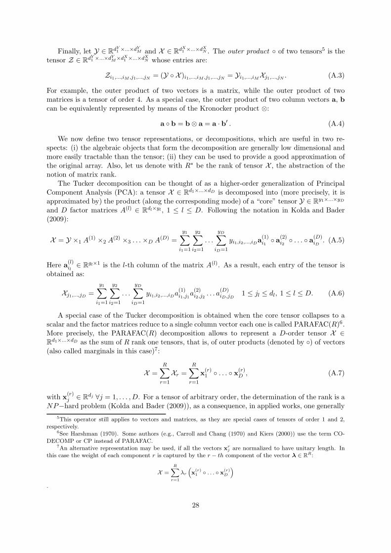
The assumed hierarchical prior distribution on the marginals of the PARAFAC(R) decompos-ition assumed for the tensor of coefficients in each regime induces a prior distribution on eachsingle entry of the tensor which is not normal. Fig. 16-18 show the empirical distribution of tworandomly chosen entries of a tensor Y ∈ R

100×100×3 whose PARAFAC decomposition is assumedwith R = 5 and R = 10, respectively. Compared to the standard normal distribution and thestandard Laplace distribution8 the prior distribution induced on the single entries of the tensoris still symmetric, but has heavier tails.

8The probability density function of the Laplace distribution with mean µ and variance 2b2 is given by:

f(x|µ, b) =1

2bexp

−|x− µ|

2b

x ∈ R, µ ∈ R, b > 0

and has kurtosis equal to 6.

29

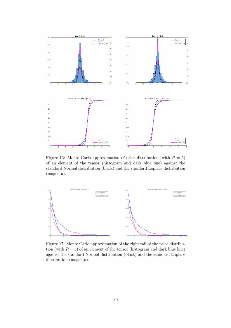
Figure 16: Monte Carlo approximation of prior distribution (with R = 5)of an element of the tensor (histogram and dark blue line) against thestandard Normal distribution (black) and the standard Laplace distribution(magenta).

Figure 17: Monte Carlo approximation of the right tail of the prior distribu-tion (with R = 5) of an element of the tensor (histogram and dark blue line)against the standard Normal distribution (black) and the standard Laplacedistribution (magenta).

30

Figure 18: Monte Carlo approximation of prior distribution (with R = 10)of an element of the tensor (histogram and dark blue line) against thestandard Normal distribution (black) and the standard Laplace distribution(magenta).

Figure 19: Monte Carlo approximation of the right tail of the prior distribu-tion (with R = 10) of an element of the tensor (histogram and dark blue line)against the standard Normal distribution (black) and the standard Laplacedistribution (magenta).

The analytical formula for the prior distribution of the generic entry gijkp,l of the fourth-ordertensor Gl ∈ R

I×J×K×P can be obtained from the PARAFAC(R) decomposition in eq. (A.7) and

31

the hierarchical prior on the marginals in eq. (13), (14), (15), (16):

π(gijkp,l) =

∫

R+

∫

SR

∫

(R+×R+)4Rπ(gijkp,l|τ,φ,w)π(τ)π(φ)π(w) dτ dφ dw , (B.1)

where SR is the standard R-simplex. The entry gijkp,l can be expressed in terms of the tensor

marginals γ(r)h,lhrl as follows:

gijkp,l =R∑

r=1

γ(r)1,i,l · γ

(r)2,j,l · γ

(r)3,k,l · γ

(r)4,p,l . (B.2)

By exploiting the conditional independence relations in the hierarchical prior of the marginalsin eq. (13), we can thus rewrite the conditional distribution π(gijkp,l|τ,φ,w) in eq. (B.1) as:

π(gijkp,l|τ,φ,w) = P

R∑

r=1

γ(r)1,i,l · γ

(r)2,j,l · γ

(r)3,k,l · γ

(r)4,p,l

, (B.3)

which is the distribution of a finite sum of independent, univariate normal distributions, centredin zero, but with individual-specific variance. The distribution of each of these products hasbeen characterised by Springer and Thompson (1970), who proved the following theorem.

Theorem B.1 (4 in Springer and Thompson (1970)). The probability density function of theproduct z =

∏Jj=1 xj of J independent Normal random variables xj ∼ N (0, σ2j ), j = 1, . . . , J , is

a Meijer G-function multiplied by a normalising constant H:

p(z|σ2j Jj=1) = H ·GJ,0J,0

z2 ·J∏

j=1

1

2σj

∣∣∣0

, (B.4)

where

H =

(2π)J/2 ·J∏

j=1

σj

−1

(B.5)

and Gm,np,q (·|·) is a Meijer G-function (with c ∈ R and s ∈ C):

Gm,np,q

(

z∣∣∣a1, . . . , apb1, . . . , bq

)

=1

2πi

∫ c+i∞

c−i∞z−s

∏mj=1 Γ(s+ bj) ·

∏nj=1 Γ(1− aj − s)

∏pj=n+1 Γ(s+ aj) ·

∏qj=m+1 Γ(1− bj − s)

ds . (B.6)

The integral is taken over a vertical line in the complex plane. Notice that in the specialcase J = 2 we have z ∼ c1P1−c2P2, with P1, P2 ∼ χ2

1 and c1 = V(x1+x2)/4, c2 = V(x1−x2)/4.

C Data augmentation

The likelihood function is:

L(X ,y|θ) =∑

s1,...,sT

T∏

t=1

p(Xt,yt|st,θ)p(st|st−1) , (C.1)

where the index l ∈ 1, . . . , L represents the regime. Through the introduction of a latentvariables s = stTt=0, we obtain the data augmented likelihood:

L(X ,y, s|θ) =T∏

t=1

L∏

l=1

L∏

h=1

[p(Xt,yt|st = l,θ)p(st = l|st−1 = h,Ξ)

]1(st=l)1(st−1=h)

. (C.2)

32

The conditional distribution of the observation given the latent variable and marginal distribu-tion of st are given by, respectively:

p(Xt,yt|st = l,θ) = fl(Xt,yt|θl) (C.3)

p(st = l|st−1 = h,Ξ) = ph . (C.4)

Considering the observation model in eq. (2) and defining Tl = t : st = l for each l = 1, . . . , L,we can rewrite eq. (C.2) as:

L(X ,y, s|θ) =T∏

t=1

L∏

l=1

[p(Xt|st = l,θ)p(yt|st = l,θ)

]1(st=l)

L∏

h=1

[p(st = l|st−1 = h,Ξ)

]1(st=l)1(st−1=h)

=

L∏

l=1

∏

t∈Tl

I∏

i=1

J∏

j=1

K∏

k=1

[

(1− ρl)expz′tgijk,l

1 + expz′tgijk,l

]xijk,t[

ρl + (1− ρl)1

1 + expz′tgijk,l

]1−xijk,t

·L∏

l=1

∏

t∈Tl

(2π)−m/2 |Σl|−1/2 exp

−1

2(yt − µl)

′Σ−1l (yt − µl)

·T∏

t=1

L∏

l=1

L∏

h=1

p1(st=l)1(st−1=h)h . (C.5)

Since the function cannot be expressed as a series of products due to the sum in the rightmostterm, we choose to further augment the data via the through the introduction of latent allocationvariables D = DlLl=1, with Dl = (dijk,l) for i = 1, . . . , I, j = 1, . . . , J and k = 1, . . . ,K. Finally,we perform another augmentation as in Polson et al. (2013), for dealing with the logistic partof the model. When the hidden chain is assumed to be first order Markov, with two possiblestates, that is L = 2, the complete data likelihood is given by:

L(X ,y,D,Ω, s|θ) = p(X ,D,Ω|s,θ)p(y|s,θ)p(s|θ)

=

T∏

t=1

p(Xt,Dt,Ωt|st,θ)p(yt|st,θ)p(st|θ) (C.6a)

=

L∏

l=1

∏

t∈Tl

I∏

i=1

J∏

j=i

K∏

k=1

p(xijk,t, dijk,t, ωijk,t|st = l, ρl,Gl)︸ ︷︷ ︸

I

(C.6b)

·

L∏

l=1

∏

t∈Tl

p(yt|st = l,µl,Σl)︸ ︷︷ ︸

II

·

p(s|Ξ)︸ ︷︷ ︸

III

(C.6c)

where we have exploited the conditional independence of X and y given the hidden chain s. Westart by analysing in detail the first term (I). The joint distribution of the observation xijk,t andthe latent variables (dijk,t, ωijk,t) is obtained from the marginal distribution of the observationin two steps. First, we augment the model by introducing the latent allocation dijk,l ∈ 0, 1 forl = 1, 2. Via this data augmentation step we are able to factorise the summation in eq. (2) foreach regime l = 1, 2. In words, the allocation latent variable is used to identify the componentof the mixture in eq. (2) from which the observation xijk,t is drawn. Secondly, we use a furtherdata augmentation step via the introduction of the latent variables ωijk,t following Polson et al.(2013), for dealing with the logistic part of the mixture.

By introducing the allocation variable dijk,t in eq. (2), for each i = 1, . . . , I, j = 1, . . . , J ,k = 1, . . . ,K and t = 1, . . . , T , we obtain:

p(xijk,t|dijk,t, st = l, ρl,Gl)

33

=[

δ0

]1dijk,t=1

·[Bern(xijk,t|ηijk,t)

]1dijk,t=0

=[

δ0(xijk,t)]dijk,t ·

(

expz′tgijk,l1 + expz′tgijk,l

)xijk,t(

1− expz′tgijk,l1 + expz′tgijk,l

)1−xijk,t

1−dijk,t

=[

δ0(xijk,t)]dijk,t ·

(expz′tgijk,l

)xijk,t(1−dijk,t)

(1 + expz′tgijk,l

)(1−dijk,t). (C.7)

p(xijk,t, dijk,t|st = l, ρl,Gl)

= ρ1dijk,t=1l ·

[

δ0(xijk,t)]1dijk,t=1

· (1− ρl)1dijk,t=0 ·

[Bern(xijk,t|ηijk,t)

]1dijk,t=0

= ρdijk,tl ·

[

δ0(xijk,t)]dijk,t · (1− ρl)

1−dijk,t ·(expz′tgijk,l

)xijk,t(1−dijk,t)

(1 + expz′tgijk,l

)(1−dijk,t). (C.8)

The marginal distribution of the allocation variable is:

p(dijk,t|st) = Bern(ρst) , (C.9)

for i = 1, . . . , I, j = 1, . . . , J , k = 1, . . . ,K and t = 1, . . . , T .By Theorem 1 in Polson et al. (2013), it is possible to decompose the ratio in the right hand

side of eq. (C.8) as follows:

(expz′tgijk,l

)xijk,t(1−dijk,t)

(1 + expz′tgijk,l

)(1−dijk,t)= 2−(1−dijk,t)

∫ ∞

0exp

−ωijk,t

2(z′tgijk,l)

2 + κijk,t(z′tgijk,l)

p(ωijk,t)dωijk,t ,

(C.10)where for every l = 1, . . . , L, i = 1, . . . , I, j = 1, . . . , J , k = 1, . . . ,K and t = 1, . . . , T :

κijk,t = xijk,t(1− dijk,t)−1− dijk,t

2= (1− dijk,t)

(

xijk,t −1

2

)

. (C.11)

Therefore we get the following conditional and joint distributions, respectively:

p(xijk,t, dijk,t|ωijk,t, st = l, ρl,Gl) =

= ρdijk,tl ·

(

0xijk,t11−xijk,t

)dij,t ·(1− ρl

2

)1−dijk,t

· exp

−ωijk,t

2(z′tgijk,l)

2 + κijk,t(z′tgijk,l)

.

(C.12)

p(xijk,t, dijk,t, ωijk,t|st = l, ρl,Gl) =

= ρdijk,tl ·

(

0xijk,t11−xijk,t

)dijk,t ·(1− ρl

2

)1−dijk,t

· exp

−ωijk,t

2(z′tgijk,l)

2 + κijk,t(z′tgijk,l)

p(ωijk,t) .

(C.13)

Finally, the marginal distribution of each latent variable ωijk,t from the data augmentationscheme follows a Polya-Gamma distribution:

ωijk,t ∼ PG(1, 0) . (C.14)

34

A continuous random variable x ∈ [0,+∞) has a Polya-Gamma distribution with parameters

b > 0, c ∈ R if the following stochastic representation holds (whereD= stands for equality in

distribution):

x ∼ PG(b, c) ⇐⇒ xD=

1

2π2

∞∑

k=1

gk(k − 1/2)2 + c2/(4π2)

(C.15)

where gk ∼ Ga(b, 1) are i.i.d. random variables. See Polson et al. (2013) for further details.The part (II) of eq. (C.6c) is the likelihood of a multivariate normal mean regression, hence:

p(yt|st = l,θ) = (2π)−m/2 |Σl|−1/2 exp

−1

2(yt − µl)

′Σ−1l (yt − µl)

. (C.16)

The last term in eq. (C.6c), according to the assumption of first order time homogeneous Markovchain, factors as9:

p(st|θ) = p(s0|Ξ)

t∏

v=1

p(sv|sv−1,Ξ) = p(s0|Ξ)

t∏

v=1

ξsv−1,sv = p(s0|Ξ)

L∏

g=1

L∏

l=1

ξNgl(s

t)g,l (C.17)

where st = (s0, . . . , st)′ and Ngl(s

t) is a function counting the number of transitions from stateg to state l in the vector st, that is (symbol # denotes the cardinality of a set): Ngl(s

t) =#st−1 = g, st = l, ∀ g, l = 1, . . . , L. The complete data likelihood for X is thus obtained byplugging, for each l = 1, . . . , L, eq. (C.13), eq. (C.16) and eq. (C.17) in eq. (C.6c):

L(X ,y,D,Ω, s|θ) =

=

L∏

l=1

∏

t∈Tl

I∏

i=1

J∏

j=1

K∏

k=1

ρdijk,tl · δ0(xijk,t)dij,t ·

(1− ρl

2

)1−dijk,t

· exp

−ωijk,t

2(z′tgijk,l)

2 + κijk,t(z′tgijk,l)

·

L∏

l=1

∏

t∈Tl

(2π)−m/2 |Σl|−1/2 exp

−1

2(yt − µl)

′Σ−1l (yt − µl)

·

T∏

t=1

I∏

i=1

J∏

j=1

K∏

k=1

p(ωijk,t)

·

L∏

g=1

L∏

l=1

ξNgl(s)g,l

· p(s0|Ξ) . (C.18)

D Computational Details

D.1 Gibbs sampler

The structure of the partially collapsed Gibbs sampler (Van Dyk and Park (2008)) is as follows:

p(s|X ,G,ρ,Ξ)

p(D|s,G,ρ)p(Ω|X , s,G)p(ψ|G,W)

p(τ |G,W,φ)

p(wh,r,l|γ(r)h,l , λl,φ, τ)

p(λl|w1,1,l, . . . , w4,R,l)

9See (Fruhwirth-Schnatter, 2006, ch.11) for more details.

35

p(γ(r)1,l |γ

(r)−1,l,G−r,l,φ, τ,W,X , s)

p(γ(r)2,l |γ

(r)−2,l,G−r,l,φ, τ,W,X , s)

p(γ(r)3,l |γ

(r)−3,l,G−r,l,φ, τ,W,X , s)

p(γ(r)4,l |γ

(r)−4,l,G−r,l,φ, τ,W,X , s)

p(ρ|s,D)

p(Ξ|s)p(µl|y, s,Σl) ∼ NM (µl, Υl)

p(Σl|y, s,µl) ∼ IWM (νl, Ψl) .

Step 1. sample latent variables from

p(s,D,Ω|X ,G,ρ,Ξ) = p(s|X ,G,ρ,Ξ) · p(D|s,G,ρ) · p(Ω|X , s,G)

– p(s|X ,G,ρ,Ξ) via FFBS (Fruhwirth-Schnatter (2006))

– p(dijk,t|st,Gt, ρt) ∼ Bern(pdijk,t)– p(ωijkv,t|xijk,t, st,Gt) ∼ PG(1, z′tgijk,st)

Step 2. sample variance hyperparameters from

p(φ, τ,W |G) = p(φ|G,W)︸ ︷︷ ︸

collapse τ

·p(τ |G,φ,W) · p(W|G,λ,φ, τ)p(λ|W)

– p(ψr|G(r),wr) ∼ GiG

2bτ,

4∑

h=1

L∑

l=1

γ(r)′

h,l γ(r)h,l

wh,r, α− n

then φr = ψr/∑

i ψi

– p(τ |G,W,φ) ∼ GiG

2bτ,

R∑

r=1

4∑

h=1

L∑

l=1

γ(r)′

h,l γ(r)h,l

φrwh,r, (α− n)R

– p(wh,r,l|γ(r)h,l , φr, τ, λl) ∼ GiG

λ2l ,γ(r)′

h,l γ(r)h,l

τφr, 1− nh

2

– p(λl|wl) ∝ λaλl+8R−1

l exp

−λlbλl

· exp

−λ

2l

2

R∑

r=1

4∑

h=1

wh,r,l

Step 3. sample tensor marginals from

p(G|X , s,φ, τ,W

)=

L∏

l=1

p(

γ(r)1,l ,γ

(r)2,l ,γ

(r)3,l ,γ

(r)4,l Rr=1

∣∣X , s,φ, τ,W

)

– p(γ(r)1,l |γ

(r)−1,l,G−r,l,φ, τ,W,X , s) ∼ Nd1(µγ1,l

,Σγ1,l)

– p(γ(r)2,l |γ

(r)−2,l,G−r,l,φ, τ,W,X , s) ∼ Nd2(µγ2,l

,Σγ2,l)

– p(γ(r)3,l |γ

(r)−3,l,G−r,l,φ, τ,W,X , s) ∼ Nd3(µγ3,l

,Σγ3,l)

36

– p(γ(r)4,l |γ

(r)−4,l,G−r,l,φ, τ,W,X , s) ∼ Nd4(µγ4,l

,Σγ4,l)

Step 4. sample switching parameters and transition matrix from

p(ρl, ξl,l|s,D) = p(ρl|s,D) · p(ξl,l|s)

– p(ρl|s,D) ∼ Be(al, bl)– p(ξl,:|s) ∼ Dir(c)

Step 5. sample the parameters of the second equation from

p(µl,Σl|y, s) = p(µl|y, s,Σl)p(Σl|y, s,µl)

– p(µl|y, s,Σl) ∼ NM (µl, Υl)

– p(Σl|y, s,µl) ∼ IWM (νl, Ψl)

The derivation of the full conditional distribution is illustrated in the following subsections.

D.2 Full conditional distribution of φr

The full conditional of the common (over r) component of the variance of the marginals fromthe PARAFAC, for each r = 1, . . . , R, can be obtained in closed form collapsing τ . This canbe done by exploiting a result in Guhaniyogi et al. (2017), which states that the posterior fullconditional of each φr can be obtained by normalising Generalised Inverse Gaussian distributedrandom variables ψr, where ψr = τφr:

p(φr|G(r),wr) =ψr

∑Ri=1 ψi

∀ r (D.1)

where for every r = 1, . . . , R:

ψr ∼ GiG

2bτ,

4∑

h=1

L∑

l=1

γ(r)′

h,l γ(r)h,l

wh,r,l, α− n

. (D.2)

In the previous notation, GiG(·) stands for the Generalized Inverse Gaussian distribution. TheGeneralized Inverse Gaussian probability density function with three parameters a > 0, b > 0,p ∈ R, for the random variable x ∈ (0,+∞), is given by:

x ∼ GiG(a, b, p) ⇒ p(x|a, b, p) =(a/b)p/2

2Kp(√ab)

xp−1 exp

−1

2

(

ax+b

x

)

(D.3)

with Kp(·) a modified Bessel function of the second type.The computation necessary for obtaining this result are as follows:

p(φ|G,W) ∝ p(φ)

∫ ∞

0p(G|W,φ, τ)p(τ) dτ (D.4a)

∝R∏

r=1

φα−1r

∫ ∞

0

R∏

r=1

4∏

h=1

L∏

l=1

(τφrwh,r,lInh)−1/2 exp

−1

2γ(r)′

h,l (τφrwh,r,lInh)−1γ

(r)h,l

37

· τaτ−1 exp

−bττ

dτ (D.4b)

=

∫ ∞

0

R∏

r=1

φα−1r

4∏

h=1

(τφrwh,r,lInh)−1 exp

−1

2

L∑

l=1

(τφrwh,r,l)−1γ

(r)′

h,l γ(r)h,l

· τaτ−1 exp

−bττ

dτ . (D.4c)

We define n = n1+n2+n3+n4 = I+J +K+Q and exploit the property det(kA) = kn det(A),for a square matrix A of size n and a scalar k. Finally, we assume:

aτ = αR (D.5)

which is allowed since the hyperparameter aτ must be positive. We can thus obtain:

∝∫ ∞

0

R∏

r=1

φα−1r

4∏

h=1

(τφrwh,r,lInh)−1 exp

−1

2

L∑

l=1

(τφrwh,r,l)−1γ

(r)′

h,l γ(r)h,l

· τaτ−1 exp

−bττ

dτ (D.6a)

∝∫ ∞

0

R∏

r=1

(τφr)α−1(τφr)

−n exp

−1

2

2bττ +

4∑

h=1

L∑

l=1

(τφrwh,r,l)−1γ

(r)′

h,l γ(r)h,l

dτ (D.6b)

=

∫ ∞

0

R∏

r=1

(τφr)α−n−1

exp

−1

2

R∑

r=1

2bττφr +

1

τφr

4∑

h=1

L∑

l=1

γ(r)′

h,l γ(r)h,l

wh,r,l

dτ (D.6c)

where in the last line we used∑R

r=1 φr = 1. It can be seen that the integrand is the kernel ofa GiG with respect to the random variable ψr = τφr. Following Guhaniyogi et al. (2017), itis possible to sample from the posterior of φr, for each r = 1, . . . , R by first sampling ψr froma GiG with kernel given in eq. (D.6c), then normalising over r, as reported in eq. (D.2)-(D.1),respectively.

As an alternative, it is possible to sample from eq. (D.2) using a Hamiltonian Monte Carlostep (Neal (2011)).

D.3 Full conditional distribution of τ

The full conditional of the global component of the variance of the PARAFAC marginals is:

p(τ |G,W,φ) ∼ GiG

2bτ,

R∑

r=1

4∑

h=1

L∑

l=1

γ(r)′

h,l γ(r)h,l

φrwh,r,l, (α− n)R

, (D.7)

The posterior full conditional distribution is derived from:

p(τ |G,W,φ) ∝ π(τ)p(G|W,φ, τ)

∝ τaτ−1 exp

−bττ R∏

r=1

4∏

h=1

L∏

l=1

∣∣τφrwh,r,lInh

∣∣−1/2

exp

−1

2γ(r)′

h,l (τφrwh,r,lInh)−1γ

(r)h,l

(D.8a)

∝ τaτ−nR−1 exp

−1

2

2bττ +

1

τ

R∑

r=1

4∑

h=1

L∑

l=1

γ(r)′

h,l γ(r)h,l

φrwh,r,l

, (D.8b)

38

which is the kernel of the GiG in eq. (D.7), once the constraint in eq. (D.5) has been taken intoaccount.

It is possible to sample from eq. (D.7) using a Hamiltonian Monte Carlo step (Neal (2011)).

D.4 Full conditional distribution of wh,r,l

The full conditional distribution of the local component of the variance of each PARAFACmarginal, for h = 1, . . . , 4, r = 1, . . . , R and l = 1, . . . , L, is given by:

p(wh,r,l|γ(r)h,l , φr, τ, λl) ∼ GiG

λ2l ,γ(r)′

h,l γ(r)h,l

τφr, 1− nh

2

, (D.9)

which follows from:

p(wh,r,l|γ(r)h,l , φr, τ, λl) ∝ π(wh,r,l|λl)p(γ(r)

h,l |wh,r,l, φr, τ) (D.10a)

∝ exp

−λ2l

2wh,r,l

∣∣τφrwh,r,lInh

∣∣−1/2

exp

−1

2γ(r)′

h,l (τφrwh,r,lInh)−1γ

(r)h,l

(D.10b)

∝ exp

−λ2l

2wh,r,l

w−nh/2h,r,l exp

−1

2

γ(r)′

h,l γ(r)h,l

τφrwh,r,l

(D.10c)

= w−nh/2h,r,l exp

−1

2

λ2lwh,r,l +1

wh,r,l

γ(r)′

h,l γ(r)h,l

τφr

. (D.10d)

It is possible to sample from eq. (D.9) using a Hamiltonian Monte Carlo step (Neal (2011)).

D.5 Full conditional distribution of λl

The full conditional distribution of λl, for l = 1, . . . , L, is given by:

p(λl|wl) ∝ λaλl+8R−1

l exp

−λlbλl

· exp

−λ

2l

2

R∑

r=1

4∑

h=1

wh,r,l

. (D.11)

It is obtained from:

p(λl|wl) ∝ π(λl)p(wl|λl) (D.12a)

∝ λalλ−1

l exp

−blλλl R∏

r=1

4∏

h=1

λ2l2

exp

−λ2l

2wh,r,l

(D.12b)

∝ λaλl+8R−1 exp

−λlbλl

· exp

−λ

2l

2

R∑

r=1

4∑

h=1

wh,r,l

. (D.12c)

Since the second exponential is always smaller than one due to the positiveness of all the para-meters λl, wh,r,l, we can sample from this distribution by means of an accept/reject algorithmusing as proposal density a Gamma distribution Ga(a, b) with parameters:

a = aλl + 8R b = bλl . (D.13)

39

Since this sampling scheme has very low acceptance rate, it is possible to sample from eq. (D.11)using a Hamiltonian Monte Carlo step (Neal (2011)).

D.6 Full conditional distribution of γ(r)h,l

For deriving the full conditional distribution of each PARAFAC marginal, γ(r)h,l , of the tensor Gl,

l = 1, . . . , L, we start by manipulating the complete data likelihood in eq. (12) with the aim of

singling out γ(r)h,l . From eq. (C.13), considering all the entries of Xt at a given t ∈ 1, . . . , T

and denoting with π(Gl) the prior distribution induced on Gl by the hierarchical prior on thePARAFAC marginals in eq. (13), the following proportionality relation holds:

p(Gl|Xt,Dt,Ωt, st = l, ρl) ∝I∏

i=1

J∏

j=1

K∏

k=1

exp

−ωijk,t

2(z′tgijk,l)

2 + κijk,t(z′tgijk,l)

p(ωijk,t)π(Gl)

=

I∏

i=1

J∏

j=1

K∏

k=1

exp

− 1

2ω−1ijk,t

[

(z′tgijk,l)2 − 2

κijk,tωijk,t

(z′tgijk,l)

]

p(ωijk,t)π(Gl)

=I∏

i=1

J∏

j=1

K∏

k=1

exp

− 1

2ω−1ijk,t

(

z′tgijk,l −κijk,tωijk,t

)2

p(ωijk,t)π(Gl).

(D.14)

Define uijk,t = κijk,t/ωijk,t, then we rewrite eq. (D.14) in more compact form as:

p(Gl|Xt,Dt,Ωt, st = l, ρl) ∝

∝ exp

−1

2

I∑

i=1

J∑

j=1

K∑

k=1

1

ω−1ijk,t

(z′tgijk,l − uijk,t

)2

·

I∏

i=1

J∏

j=1

K∏

k=1

p(ωijk,t) · π(Gl)

= exp

−1

2

I∑

i=1

(Gl ×4 zt − Ut)′i diag

(ωi:,t

)(Gl ×4 zt − Ut)i

·

I∏

i=1

J∏

j=1

K∏

k=1

p(ωijk,t) · π(Gl)

= exp

−1

2

(vec (Gl ×4 zt)− vec (Ut)

)′diag

(vec (Ωt)

) (vec (Gl ×4 zt)− vec (Ut)

)

·I∏

i=1

J∏

j=1

K∏

k=1

p(ωijk,t) · π(Gl)

= f (Gl, zt,Ut,Ωt) ·I∏

i=1

J∏

j=1

K∏

k=1

p(ωijk,t) · π(Gl) , (D.15)

where f(·) is a function which contains the kernel of a multivariate normal distribution withrespect to the variable vec (Gl ×4 zt).

Given the proportionality relation conditional on the latent variable st, the last step in themanipulation of the likelihood function consists in rewriting the complete data likelihood. Thus,considering eq. (12) and (D.15) we obtain the proportionality relation:

L(X ,D,Ω, s|θ) =L∏

l=1

∏

t∈Tl

p(Xt,Dt,Ωt, st|θ) ∝L∏

l=1

∏

t∈Tl

f (Gst , zt,Ut,Ωt) . (D.16)

40

We are now ready to compute the full conditional distributions of each vector γ(r)h,l , h = 1, . . . , 4,

l = 1, . . . , L and r = 1, . . . , R. To this aim, notice that:

Gl =R∑

r=1

γ(r)1,l γ

(r)2,l γ

(r)3,l γ

(r)4,l = G(r)

l + G(−r)l , (D.17)

where we have defined:

G(r)l = γ

(r)1,l γ

(r)2,l γ

(r)3,l γ

(r)4,l (D.18a)

G(−r)l =

R∑

v=1v 6=r

G(v)l . (D.18b)

By exploiting the definitions of mode-n product and PARAFAC decomposition, we obtain:

Gl,t = Gl ×4 zt =R∑

r=1

(

γ(r)1,l γ

(r)2,l γ

(r)3,l

)

〈γ(r)4,l , zt〉 =

R∑

r=1

G(r)l,t . (D.19)

Here 〈·, ·〉 denotes the standard inner product in the Euclidean space Rn. Since the latter is a

scalar, we have that:

gl,t = vec(Gl,t

)= vec (Gl ×4 zt) =

R∑

r=1

vec(

G(r)l,t

)

=

R∑

r=1

g(r)l,t . (D.20)

The vectorisation of a tensor can be expressed in the following way, which is a generalisation ofa well known property holding for matrices: it consists in stacking in a column vector all thevectorised slices of the tensor. For the sake of clarity, let α1 ∈ R

I , α2 ∈ RJ and α3 ∈ R

K andlet the tensor A = α1 α2 α3. Denote A::k ∈ R

I×J the k-th frontal slice of the tensor A. Then,by applying the properties of Kronecker product, ⊗, and of the vectorization operator, vec, weobtain10:

vec (A) = vec (α1 α2 α3) =[

vec (A::1)′ , . . . , vec (A::K)′

]′

=[

vec (α1 α2)′ α3,1, . . . , vec (α1 α2)

′ α3,K

]′

10The outer product and Kronecker products are two operators acting on:

: Rn1 × . . .× RnK → R

n1×...×nK

⊗ : Rn1×m1 × Rn2×m2 → R

n1n2×m1m2 .

Notice that the Kronecker product is defined on the space of matrices (and vectors, as a particular case), whilethe outer product is defined on arrays of possible different number of dimensions (e.g. it is defined between twovectors, and returns a matrix, as well as between a vector and a matrix, yielding a third order tensor). In practice,in the particular case aring when dealing with two vectors u ∈ R

n and v ∈ Rm, their outer product and Kronecker

product are related and given by, respectively:

u v = uv′ ∈ R

n×m

u⊗ v = vec(

vu′)

= vec (v u) ∈ Rnm

.

For two matrices A ∈ Rm×n and B ∈ R

n×k it holds:

vec (AB) = (Ik ⊗A) vec (B) = (B′ ⊗ Im) vec (A) ∈ Rmk×1

.

Moreover, if n = 1 then B is a row vector of length k, as a consequence B′ = vec (B) ∈ Rk×1. See (Cichocki et al.,

2009, p.31).

41

= α3 ⊗ vec (α1 α2) = α3 ⊗ vec(α1α

′2

). (D.21)

The use of the same property allows to rewrite eq. (D.21) in three equivalent ways, each onewritten as a product of a matrix and one of the vectors α1,α2,α3, respectively. In fact, wehave:

vec (A) = α3 ⊗ vec(α1α

′2

)= α3 ⊗ (α2 ⊗ II) vec (α1) = (α3 ⊗α2 ⊗ II)α1 (D.22)

vec (A) = α3 ⊗ vec(α1α

′2

)= α3 ⊗

[

(IJ ⊗α1) vec(α′

2

)]

= (α3 ⊗ IJ ⊗α1)α2 (D.23)

vec (A) = α3 ⊗ vec(α1α

′2

)= vec

(

vec(α1α

′2

)α′

3

)

=(

IK ⊗ vec(α1α

′2

))

vec(α′

3

)

=(

IK ⊗ vec(α1α

′2

))

α3 = (IK ⊗α2 ⊗α1)α3 . (D.24)

The first line represents a product between the matrix α3 ⊗ α2 ⊗ II ∈ RIJK×I and the vector

α1, the second is a product between the matrix α3 ⊗ IJ ⊗ α1 ∈ RIJK×J and the vector α2.

Finally, the last row is a product between the matrix IK ⊗ α2 ⊗ α1 ∈ RIJK×K and the vector

α3.Starting from eq. (D.20), we can apply for γ

(r)1,l , . . . ,γ

(r)3,l the same argument as for α1, . . . ,α3,

with the aim of manipulating the likelihood function and obtain three different expressions where

the dependence on γ(r)1,l ,γ

(r)2,l ,γ

(r)3,l , respectively, is made explicit. This will then be used later on

for deriving the posterior full conditional distributions of the PARAFAC marginals. Thus, fromeq. (D.20) we have:

g(r)l,t = vec

(

G(r)l,t

)

= 〈γ(r)4,l , zt〉 vec

(

γ(r)1,l γ

(r)2,l γ

(r)3,l

)

= vec(

γ(r)1,l γ

(r)2,l γ

(r)3,l

)

z′tγ(r)4,l = A4γ

(r)4,l ,

(D.25)where:

A4 = vec(

γ(r)1,l γ

(r)2,l γ

(r)3,l

)

z′t . (D.26)

Exploiting eq. (D.22) we have:

g(r)l,t = vec

(

G(r)l,t

)

= 〈γ(r)4,l , zt〉

(

γ(r)3,l ⊗ γ

(r)2,l ⊗ II

)

γ(r)1,l = A1γ

(r)1,l , (D.27)

with:A1 = 〈γ(r)

4,l , zt〉(

γ(r)3,l ⊗ γ

(r)2,l ⊗ II

)

. (D.28)

Exploiting eq. (D.23) we have:

g(r)l,t = vec

(

G(r)l,t

)

= 〈γ(r)4,l , zt〉

(

γ(r)3,l ⊗ IJ ⊗ γ(r)

1,l

)

γ(r)2,l = A2γ

(r)2,l , (D.29)

with:A2 = 〈γ(r)

4,l , zt〉(

γ(r)3,l ⊗ IJ ⊗ γ(r)

1,l

)

. (D.30)

Finally, using eq. (D.24) we obtain:

g(r)l,t = vec

(

G(r)l,t

)

= 〈γ(r)4,l , zt〉

(

IK ⊗ γ(r)2,l ⊗ γ

(r)1,l

)

γ(r)3,l = A3γ

(r)3,l , (D.31)

with:A3 = 〈γ(r)

4,l , zt〉(

IK ⊗ γ(r)2,l ⊗ γ

(r)1,l

)

. (D.32)

By using the definition of f(Gl, zt,U (l)t ,Ωt), eq. (D.20) and the notation of eq. (D.17) we can

thus write:

vec (Gl ×4 zt) = g(r)l,t +

R∑

v=1v 6=r

g(v)l,t = g

(r)l,t + g

(−r)l,t . (D.33)

42

From eq. (D.16), by focusing on regime l ∈ 1, . . . , L, we get:

L(X ,D,Ω, s|θ) ∝

∝ exp

−1

2

(vec (Gl ×4 zt)− vec (Ut)

)′diag

(vec (Ωt)

) (vec (Gl ×4 zt)− vec (Ut)

)

= exp

−1

2

(

g(r)l,t + g

(−r)l,t − ut

)′Ωt

(

g(r)l,t + g

(−r)l,t − ut

)

(D.34)

where, for reducing the burden of notation, we have defined:

ut = vec (Ut) (D.35)

Ωt = diag(vec (Ωt)

). (D.36)

We can now single out a specific component G(r)l of the PARAFAC decomposition of the tensor

G, which is incorporated in g(r)l,t . In fact, we can manipulate the function in eq. (D.34) with the

aim of finding a proportionality relation, as follows:

L(X ,D,Ω, s|θ) ∝∏

t∈Tl

exp

−1

2

[

g(r)′

l,t Ωtg(r)l,t + g

(r)′

l,t Ωt(g(−r)l,t − ut)

+ (g(−r)l,t − ut)

′Ωtg(r)l,t + (g

(−r)l,t − ut)

′Ωt(g(−r)l,t − ut)

]

∝∏

t∈Tl

exp

−1

2

[

g(r)′

l,t Ωtg(r)l,t − 2(ut − g

(−r)l,t )′Ωtg

(r)l,t

]

. (D.37)

D.6.1 Full conditional distribution of γ(r)1,l

The full conditional distribution of γ(r)1,l is given by:

p(γ(r)1,l |X ,D,Ω, s,γ(r)

2,l ,γ(r)3,l ,γ

(r)4,l ,G

(−r)l , w1,r, φr, τ) ∼ NI(ζ

r1,l, Λ

r1,l) (D.38)

where:

Λr1,l =

(τφrw1,rII

)−1+∑

t∈Tl

(

Σ(r)

1,l,t

)−1

−1

(D.39a)

ζr1,l = Λ

r′

1,l

ζr′

1,l

(τφrw1,rII

)−1+∑

t∈Tl

µ(r)′

1,l,t

(

Σ(r)

1,l,t

)−1

′

. (D.39b)

By exploiting the rightmost term in the equality chain in eq. (D.27), we can simplify the twoaddenda in eq. (D.37) as:

g(r)′

l,t Ωtg(r)l,t =

(

A1γ(r)1,l

)′Ωt

(

A1γ(r)1,l

)

= 〈γ(r)4,l , zt〉γ

(r)′

1,l

(

γ(r)3,l ⊗ γ

(r)2,l ⊗ II

)′Ωt

(

γ(r)3,l ⊗ γ

(r)2,l ⊗ II

)

γ(r)1,l 〈γ

(r)4,l , zt〉

= γ(r)′

1,l

[(

γ(r)′

3,l ⊗ γ(r)′

2,l ⊗ I′I

)

Ωt

(

γ(r)3,l ⊗ γ

(r)2,l ⊗ II

)

(〈γ(r)4,l , zt〉)2

]

γ(r)1,l

43

= γ(r)′

1,l

(

Σ(r)

1,l,t

)−1

γ(r)1,l . (D.40)

and

−2(ut − g(−r)l,t )′Ωtg

(r)l,t = −2(ut − g

(−r)l,t )′Ωt

(

γ(r)3,l ⊗ γ

(r)2,l ⊗ II

)

γ(r)1,l 〈γ

(r)4,l , zt〉

= −2〈γ(r)4,l , zt〉(ut − g

(−r)l,t )′Ωt

(

γ(r)3,l ⊗ γ

(r)2,l ⊗ II

)

γ(r)1,l

= −2µ(r)′

1,l,t

(

Σ(r)

1,l,t

)−1

γ(r)1,l . (D.41)

Now, by applying Bayes’ rule and plugging eq. (D.40) and eq. (D.41) into eq. (D.37) we get:

p(γ(r)1,l |−) ∝ L(X ,D,Ω, s|θ)π(γ(r)

1,l |w1,:,φ, τ)

∝∏

t∈Tl

exp

−1

2

[

γ(r)′

1,l

(

Σ(r)

1,l,t

)−1

γ(r)1,l − 2µ

(r)′

1,l,t

(

Σ(r)

1,l,t

)−1

γ(r)1,l

]

· exp

−1

2

[

γ(r)′

1,l

(

Λr1,l

)−1γ(r)1,l − 2ζ

r′

1,l

(

Λr1,l

)−1γ(r)1,l

]

= exp

−1

2

[∑

t∈Tl

(

γ(r)′

1,l

(

Σ(r)

1,l,t

)−1

γ(r)1,l − 2µ

(r)′

1,l,t

(

Σ(r)

1,l,t

)−1

γ(r)1,l

)

+

(

γ(r)′

1,l

(

Λr1,l

)−1γ(r)1,l − 2ζ

r′

1,l

(

Λr1,l

)−1γ(r)1,l

)]

= exp

−1

2

[

γ(r)′

1,l

∑

t∈Tl

(

Σ(r)

1,l,t

)−1

γ(r)1,l − 2

∑

t∈Tl

µ(r)′

1,l,t

(

Σ(r)

1,l,t

)−1

γ(r)1,l

+ γ(r)′

1,l

(

Λr1,l

)−1γ(r)1,l − 2ζ

r′

1,l

(

Λr1,l

)−1γ(r)1,l

]

= exp

−1

2

[

γ(r)′

1,l

(

Λr1,l

)−1+∑

t∈Tl

(

Σ(r)

1,l,t

)−1

γ(r)1,l

− 2

ζr′

1,l

(

Λr1,l

)−1+∑

t∈Tl

µ(r)′

1,l,t

(

Σ(r)

1,l,t

)−1

γ(r)1,l

]

. (D.42)

This is the kernel of a multivariate normal distribution with parameters:

Λr1,l =

(τφrw1,rII

)−1+∑

t∈Tl

(

Σ(r)

1,l,t

)−1

−1

(D.43a)

ζr1,l = Λ

r′

1,l

ζr′

1,l

(τφrw1,rII

)−1+∑

t∈Tl

µ(r)′

1,l,t

(

Σ(r)

1,l,t

)−1

′

. (D.43b)

D.6.2 Full conditional distribution of γ(r)2,l

The full conditional distribution of γ(r)2,l is given by:

p(γ(r)2,l |X ,D,Ω, s,γ(r)

1,l ,γ(r)3,l ,γ

(r)4,l ,G

(−r)l , w2,r, φr, τ) ∼ NJ(ζ

r2,l, Λ

r2,l) (D.44)

44

where:

Λr2,l =

(τφrw2,rIJ

)−1+∑

t∈Tl

(

Σ(r)

2,l,t

)−1

−1

(D.45a)

ζr2,l = Λ

r′

2,l

ζr′

2,l

(τφrw2,rIJ

)−1+∑

t∈Tl

µ(r)′

2,l,t

(

Σ(r)

2,l,t

)−1

′

. (D.45b)

By exploiting the central term in the equality chain in eq. (D.29), we can simplify the twoaddenda in eq. (D.37) as:

g(r)′

l,t Ωtg(r)l,t =

(

A2γ(r)2,l

)′Ωt

(

A2γ(r)2,l

)

= 〈γ(r)4,l , zt〉γ

(r)′

2,l

(

γ(r)3,l ⊗ IJ ⊗ γ(r)

1,l

)′Ωt

(

γ(r)3,l ⊗ IJ ⊗ γ(r)

1,l

)

γ(r)2,l 〈γ

(r)4,l , zt〉

= γ(r)′

2,l

[(

γ(r)′

3,l ⊗ I′J ⊗ γ(r)′

1,l

)

Ωt

(

γ(r)3,l ⊗ IJ ⊗ γ(r)

1,l

)

(〈γ(r)4,l , zt〉)2

]

γ(r)2,l

= γ(r)′

2,l

(

Σ(r)

2,l,t

)−1

γ(r)2,l . (D.46)

and

−2(ut − g(−r)l,t )′Ωtg

(r)l,t = −2(ut − g

(−r)l,t )′Ωt〈γ(r)

4,l , zt〉(

γ(r)3,l ⊗ IJ ⊗ γ(r)

1,l

)

γ(r)2,l

= −2〈γ(r)4,l , zt〉(ut − g

(−r)l,t )′Ωt

(

γ(r)3,l ⊗ IJ ⊗ γ(r)

1,l

)

γ(r)2,l

= −2µ(r)′

2,l,t

(

Σ(r)

2,l,t

)−1

γ(r)2,l . (D.47)

Now, by applying Bayes’ rule and plugging eq. (D.46) and eq. (D.47) into eq. (D.37) we get:

p(γ(r)2,l |−) ∝ L(X ,D,Ω, s|θ)π(γ(r)

2,l |w2,:,φ, τ)

∝∏

t∈Tl

exp

−1

2

[

γ(r)′

2,l

(

Σ(r)

2,l,t

)−1

γ(r)2,l − 2µ

(r)′

2,l,t

(

Σ(r)

2,l,t

)−1

γ(r)2,l

]

· exp

−1

2

[

γ(r)′

2,l

(

Λr2,l

)−1γ(r)2,l − 2ζ

r′

2,l

(

Λr2,l

)−1γ(r)2,l

]

= exp

−1

2

[∑

t∈Tl

(

γ(r)′

2,l

(

Σ(r)

2,l,t

)−1

γ(r)2,l − 2µ

(r)′

2,l,t

(

Σ(r)

2,l,t

)−1

γ(r)2,l

)

+

(

γ(r)′

2,l

(

Λr2,l

)−1γ(r)2,l − 2ζ

r′

2,l

(

Λr2,l

)−1γ(r)2,l

)]

= exp

−1

2

[

γ(r)′

2,l

∑

t∈Tl

(

Σ(r)

2,l,t

)−1

γ(r)2,l − 2

∑

t∈Tl

µ(r)′

2,l,t

(

Σ(r)

2,l,t

)−1

γ(r)2,l

+ γ(r)′

2,l

(

Λr2,l

)−1γ(r)2,l − 2ζ

r′

2,l

(

Λr2,l

)−1γ(r)2,l

]

= exp

−1

2

[

γ(r)′

2,l

(

Λr2,l

)−1+∑

t∈Tl

(

Σ(r)

2,l,t

)−1

γ(r)2,l

45

− 2

ζr′

2,l

(

Λr2,l

)−1+∑

t∈Tl

µ(r)′

2,l,t

(

Σ(r)

2,l,t

)−1

γ(r)2,l

]

. (D.48)

This is the kernel of a multivariate normal distribution with parameters:

Λr2,l =

(τφrw2,rIJ

)−1+∑

t∈Tl

(

Σ(r)

2,l,t

)−1

−1

(D.49a)

ζr2,l = Λ

r′

2,l

ζr′

2,l

(τφrw2,rIJ

)−1+∑

t∈Tl

µ(r)′

2,l,t

(

Σ(r)

2,l,t

)−1

′

. (D.49b)

D.6.3 Full conditional distribution of γ(r)3,l

The full conditional distribution of γ(r)3,l is given by:

p(γ(r)3,l |X ,D,Ω, s,γ(r)

1,l ,γ(r)2,l ,γ

(r)4,l ,G

(−r)l , w3,r, φr, τ) ∼ NK(ζ

r3,l, Λ

r3,l) (D.50)

where:

Λr3,l =

(τφrw3,rIK

)−1+∑

t∈Tl

(

Σ(r)

3,l,t

)−1

−1

(D.51a)

ζr3,l = Λ

r′

3,l

ζr′

3,l

(τφrw3,rIK

)−1+∑

t∈Tl

µ(r)′

3,l,t

(

Σ(r)

3,l,t

)−1

′

. (D.51b)

By exploiting the rightmost term in the equality chain in eq. (D.31), we can simplify the twoaddenda in eq. (D.37) as:

g(r)′

l,t Ωtg(r)l,t =

(

A3γ(r)3,l

)′Ωt

(

A3γ(r)3,l

)

= 〈γ(r)4,l , zt〉γ

(r)′

3,l

(

IK ⊗ γ(r)2,l ⊗ γ

(r)1,l

)′Ωt

(

IK ⊗ γ(r)2,l ⊗ γ

(r)1,l

)

γ(r)3,l 〈γ

(r)4,l , zt〉

= γ(r)′

3,l

[(

I′K ⊗ γ(r)′

2,l ⊗ γ(r)′

1,l

)

Ωt

(

IK ⊗ γ(r)2,l ⊗ γ

(r)1,l

)

(〈γ(r)4,l , zt〉)2

]

γ(r)3,l

= γ(r)′

3,l

(

Σ(r)

3,l,t

)−1

γ(r)3,l . (D.52)

and

−2(ut − g(−r)l,t )′Ωtg

(r)l,t = −2(ut − g

(−r)l,t )′Ωt

(

IK ⊗ γ(r)2,l ⊗ γ

(r)1,l

)

γ(r)3,l 〈γ

(r)4,l , zt〉

= −2〈γ(r)4,l , zt〉(ut − g

(−r)l,t )′Ωt

(

IK ⊗ γ(r)2,l ⊗ γ

(r)1,l

)

γ(r)3,l

= −2µ(r)′

3,l,t

(

Σ(r)

3,l,t

)−1

γ(r)3,l . (D.53)

Now, by applying Bayes’ rule and plugging eq. (D.52) and eq. (D.53) into eq. (D.37) we get:

p(γ(r)3,l |−) ∝ L(X ,D,Ω, s|θ)π(γ(r)

3,l |w3,:,φ, τ)

46

∝∏

t∈Tl

exp

−1

2

[

γ(r)′

3,l

(

Σ(r)

3,l,t

)−1

γ(r)3,l − 2µ

(r)′

3,l,t

(

Σ(r)

3,l,t

)−1

γ(r)3,l

]

· exp

−1

2

[

γ(r)′

3,l

(

Λr3,l

)−1γ(r)3,l − 2ζ

r′

3,l

(

Λr3,l

)−1γ(r)3,l

]

= exp

−1

2

[∑

t∈Tl

(

γ(r)′

3,l

(

Σ(r)

3,l,t

)−1

γ(r)3,l − 2µ

(r)′

3,l,t

(

Σ(r)

3,l,t

)−1

γ(r)3,l

)

+

(

γ(r)′

3,l

(

Λr3,l

)−1γ(r)3,l − 2ζ

r′

3,l

(

Λr3,l

)−1γ(r)3,l

)]

= exp

−1

2

[

γ(r)′

3,l

∑

t∈Tl

(

Σ(r)

3,l,t

)−1

γ(r)3,l − 2

∑

t∈Tl

µ(r)′

3,l,t

(

Σ(r)

3,l,t

)−1

γ(r)3,l

+ γ(r)′

3,l

(

Λr3,l

)−1γ(r)3,l − 2ζ

r′

3,l

(

Λr3,l

)−1γ(r)3,l

]

= exp

−1

2

[

γ(r)′

3,l

(

Λr3,l

)−1+∑

t∈Tl

(

Σ(r)

3,l,t

)−1

γ(r)3,l

− 2

ζr′

3,l

(

Λr3,l

)−1+∑

t∈Tl

µ(r)′

3,l,t

(

Σ(r)

3,l,t

)−1

γ(r)3,l

]

. (D.54)

This is the kernel of a multivariate normal distribution with parameters:

Λr3,l =

(τφrw3,rIK

)−1+∑

t∈Tl

(

Σ(r)

3,l,t

)−1

−1

(D.55a)

ζr3,l = Λ

r′

3,l

ζr′

3,l

(τφrw3,rIK

)−1+∑

t∈Tl

µ(r)′

3,l,t

(

Σ(r)

3,l,t

)−1

′

. (D.55b)

D.6.4 Full conditional distribution of γ(r)4,l

The full conditional distribution of γ(r)4,l is given by:

p(γ(r)4,l |X ,D,Ω, s,γ(r)

1,l ,γ(r)2,l ,γ

(r)3,l ,G

(−r)l , w4,r, φr, τ) ∼ NQ(ζ

r4,l, Λ

r4,l) (D.56)

where:

Λr4,l =

(τφrw4,rIQ

)−1+∑

t∈Tl

(

Σ(r)

4,l,t

)−1

−1

(D.57a)

ζr4,l = Λ

r′

4,l

ζr′

4,l

(τφrw4,rIQ

)−1+∑

t∈Tl

µ(r)′

4,l,t

(

Σ(r)

4,l,t

)−1

′

. (D.57b)

By exploiting the central term in the equality chain in eq. (D.25), we can simplify the twoaddenda in eq. (D.37) as:

g(r)′

l,t Ωtg(r)l,t =

(

A4γ(r)4,l

)′Ωt

(

A4γ(r)4,l

)

47

= γ(r)′

4,l zt vec(

γ(r)1,l γ

(r)2,l γ

(r)3,l

)

Ωt vec(

γ(r)1,l γ

(r)2,l γ

(r)3,l

)

z′tγ(r)4,l

= γ(r)′

4,l

(

Σ(r)

4,l,t

)−1

γ(r)4,l . (D.58)

and

−2(ut − g(−r)l,t )′Ωtg

(r)l,t = −2(ut − g

(−r)l,t )′Ωt vec

(

γ(r)1,l γ

(r)2,l γ

(r)3,l

)

z′tγ(r)4,l

= −2µ(r)′

4,l,t

(

Σ(r)

4,l,t

)−1

γ(r)4,l . (D.59)

Now, by applying Bayes’ rule and plugging eq. (D.58) and eq. (D.59) into eq. (D.37) we get:

p(γ(r)4,l |−) ∝ L(X ,D,Ω, s|θ)π(γ(r)

4,l |w4,:,φ, τ)

∝∏

t∈Tl

exp

−1

2

[

γ(r)′

4,l

(

Σ(r)

4,l,t

)−1

γ(r)4,l − 2µ

(r)′

4,l,t

(

Σ(r)

4,l,t

)−1

γ(r)4,l

]

· exp

−1

2

[

γ(r)′

4,l

(

Λr4,l

)−1γ(r)4,l − 2ζ

r′

4,l

(

Λr4,l

)−1γ(r)4,l

]

= exp

−1

2

[∑

t∈Tl

(

γ(r)′

3,l

(

Σ(r)

4,l,t

)−1

γ(r)4,l − 2µ

(r)′

4,l,t

(

Σ(r)

4,l,t

)−1

γ(r)4,l

)

+

(

γ(r)′

4,l

(

Λr4,l

)−1γ(r)4,l − 2ζ

r′

4,l

(

Λr4,l

)−1γ(r)4,l

)]

= exp

−1

2

[

γ(r)′

4,l

∑

t∈Tl

(

Σ(r)

4,l,t

)−1

γ(r)4,l − 2

∑

t∈Tl

µ(r)′

4,l,t

(

Σ(r)

4,l,t

)−1

γ(r)4,l

+ γ(r)′

4,l

(

Λr4,l

)−1γ(r)4,l − 2ζ

r′

4,l

(

Λr4,l

)−1γ(r)4,l

]

= exp

−1

2

[

γ(r)′

4,l

(

Λr4,l

)−1+∑

t∈Tl

(

Σ(r)

4,l,t

)−1

γ(r)4,l

− 2

ζr′

4,l

(

Λr4,l

)−1+∑

t∈Tl

µ(r)′

4,l,t

(

Σ(r)

4,l,t

)−1

γ(r)4,l

]

. (D.60)

This is the kernel of a multivariate normal distribution with parameters:

Λr4,l =

(τφrw4,rIQ

)−1+∑

t∈Tl

(

Σ(r)

4,l,t

)−1

−1

(D.61a)

ζr4,l = Λ

r′

4,l

ζr′

4,l

(τφrw4,rIQ

)−1+∑

t∈Tl

µ(r)′

4,l,t

(

Σ(r)

4,l,t

)−1

′

. (D.61b)

D.7 Full conditional distribution of ωijk,t

The full conditional distribution for the latent variable ωijk,t for every i = 1, . . . , I, j = 1, . . . , J ,k = 1, . . . ,K and t = 1, . . . , T :

p(ωijk,t|xijk,t, st,Gst) ∼ PG(1, z′tgijk,st) . (D.62)

48

To shorten the notation, define ψijk,t = z′tgijk,st. The full conditional is derived by integratingout the latent allocation variable dijk,t, as follows:

p(ωijk,t|xijk,t, st,Gst)

=

∫

D

∫

ρp(ωijk,t, dijk,t|xijk,t, st,Gst , ρst)p(ρst) dρstddijk,t

=

∫

D

∫

ρ

p(xijk,t, dij,t|ωijk,t, st,Gst , ρst)p(ωijk,t)p(ρst)∫

Ω p(xijk,t, ωijk,t, dijk,t|st,Gst , ρst) dωijk,tdρstddijk,t

=

∫

D

∫

ρ

p(xijk,t, ωijk,t, dijk,t|st,Gst , ρst)

p(xijk,t, dijk,t|st,Gst , ρst)p(ρst) dρstddijk,t

=

∫

D

∫

ρ

(

ρstδ0(xijk,t))dijk,t

(1−ρst

2

)dijk,texp

−ωijk,t

2 ψ2ijk,t + κijk,tψijk,t

p(ωijk,t)p(ρst)(

ρstδ0(xijk,t))dijk,t

(1−ρst

2

)dijk,t(expψijk,txijk,t/(1 + expψijk,t))1−dijk,t

dρstddijk,t

=

∫

D

∫

ρexpκ(st)ijk,tψijk,t

expψijk,txijk,t(1− dijk,t)(1 + expψijk,t)1−dijk,t

exp

−ωijk,t

2ψ2ijk,t

p(ωijk,t)p(ρst) dρstddijk,t

=

∫

D

∫

ρ

[

1 + expψijk,texpψijk,txijk,t

· expψijk,txijk,texpψijk,t/2

]1−dijk,t [

exp−ψ2ijk,tωijk,t/2p(ωijk,t)

]

p(ρst) dρstddijk,t

=

(

1 +1 + expψijk,texpψijk,t/2

)[

exp−ψ2ijk,tωijk,t/2p(ωijk,t)

]

∝ exp−ψ2ijk,tωijk,t/2p(ωijk,t) . (D.63)

Since p(ωijk,t) ∼ PG(1, 0), by Theorem 1 in Polson et al. (2013) the result follows.

D.8 Full conditional distribution of dijk,t

The full conditional posterior probabilities for the latent allocation variables dijk,t, which selectthe component of the mixture in eq. (3), for each t = 1, . . . , T and for every i = 1, . . . , I,j = 1, . . . , J and k = 1, . . . ,K, are given by:

p(dijk,t = 1|X , s,Gst ,ρst) =p(dijk,t = 1|X , s,Gst ,ρst)

p(dijk,t = 1|X , s,Gst ,ρst) + p(dijk,t = 0|X , s,Gst ,ρst)(D.64a)

p(dij,t = 0|X , s,Gst ,ρst) =p(dijk,t = 0|X , s,Gst ,ρst)

p(dijk,t = 1|X , s,Gst ,ρst) + p(dijk,t = 0|X , s,Gst ,ρst). (D.64b)

The unnormalised posterior probabilities are given by:

p(dijk,t = 1|X , s,Gst ,ρst) = ρstδ0(xijk,t) (D.65a)

p(dijk,t = 0|X , s,Gst ,ρst) = (1− ρst)exp

(z′tgijk,st)xijk,t

1 + expz′tgijk,st. (D.65b)

We have obtained the result starting from eq. (12) after having integrated out the latent variablesΩ, as follows:

p(dijk,t|X , s,Gst ,ρst) ∝ p(X , s|Gst ,ρst, dijk,t)π(dijk,t)

= ρdijk,tst δ0(xijk,t)

dijk,t(1− ρst)1−dijk,t

(expz′tgijk,st)xijk,t(1−dijk,t)

(1 + expz′tgijk,st)(1−dijk,t)

=[

ρstδ0(xijk,t)]dijk,t

[

(1− ρst)(expz′tgijk,st)xijk,t

1 + expz′tgijk,st

]1−dijk,t

. (D.66)

49

D.9 Full conditional distribution of ρl

For each regime l = 1, . . . , L, the full conditional distribution for the mixing probability ρl ofthe observation model in eq (2) is given by:

p(ρl|X ,D, s) = p(ρl|D, s) ∼ Be(al, bl) , (D.67)

with:

al = N l1 + aρl (D.68a)

bl = N l0 + b

ρl . (D.68b)

We get this result starting from eq. (12) and integrating out the latent variables Ω, as follows:

p(ρl|X ,D, s) ∝ π(ρl)

∫

GL(X ,D, s|ρl,Gl)p(Gl) dGl

∝[∫

G

∏

t∈Tl

I∏

i=1

J∏

j=1

K∏

k=1

ρdijk,tl ·

[

δ0(xijk,t)]dijk,t · (1− ρl)

1−dijk,t

·(expz′tgijk,l

)xijk,t(1−dijk,t)

(1 + expz′tgijk,l

)(1−dijk,t)dGl

]

· ρaρl−1

l (1− ρl)bρl −1

∝

∏

t∈Tl

I∏

i=1

J∏

j=1

K∏

k=1

ρdijk,tl (1− ρl)

1−dijk,t

ρaρl−1

l (1− ρl)bρl −1

= ρN l

1l (1− ρl)

N l0ρ

aρl−1

l (1− ρl)bρl −1

= ρN l

1+aρl−1

l (1− ρl)N l

0+bρl −1 , (D.69)

where we have defined the counting variables, for every l = 1, . . . , L:

N l1 =

∑

t∈Tl

I∑

i=1

J∑

j=1

K∑

k=1

1dijk,t = 1 (D.70a)

N l0 =

∑

t∈Tl

I∑

i=1

J∑

j=1

K∑

k=1

1dijk,t = 0 . (D.70b)

D.10 Full conditional distribution of µl

The full conditional distribution for the intercept term of the second equation of the model isgiven by:

p(µl|y, s,Σl) ∼ NM(µl, Υl) , (D.71)

with:

µl = Υ′l

µ′lΥ

−1l +

∑

t∈Tl

y′tΣ−1l

′

, (D.72a)

Υl =[

TlΣ−1l +Υ

−1l

]−1, (D.72b)

for each regime l = 1, . . . , L. We have derived the updated hyperparameters from:

p(µl|y, s,Σl) ∝ π(µl)p(y|s,Σl,µl)

50

∝ exp

−1

2(µl − µl)

′Υ−1l (µl − µl)

∏

t∈Tl

exp

−1

2(yt − µl)

′Σ−1l (yt − µl)

∝ exp

−1

2

µ′lΥ

−1l µl − 2µ′

lΥ−1l µl +

∑

t∈Tl

µ′lΣ

−1l µl − 2y′

tΣ−1l µl

∝ exp

−1

2

µ

′l

(

TlΣ−1l +Υ

−1l

)

µl − 2

∑

t∈Tl

y′tΣ

−1l + µ′

lΥ−1l

µl

. (D.73)

D.11 Full conditional distribution of Σl

The full conditional distribution for the covariance of the error term of the second equation ofthe model is given by:

p(Σl|y, s,µl) ∼ IWM (νl, Ψl) , (D.74)

with:

ν l = νl + Tl , (D.75a)

Ψl = Ψl +∑

t∈Tl

(yt − µl)(yt − µl)′ , (D.75b)

for each regime l = 1, . . . , L. We have derived the updated hyperparameters from:

p(Σl|y, s,µl) ∝ π(Σl)p(y|s,µl,Σl)

∝ |Σl|−νl+m−1

2 exp

−1

2tr(

ΨlΣ−1l

)∏

t∈Tl

|Σl|−1/2 exp

−1

2(yt − µl)

′Σ−1l (yt − µl)

= |Σl|−νl+m−1+Tl

2 exp

−1

2

tr(

ΨlΣ−1l

)

+∑

t∈Tl

(yt − µl)′Σ−1

l (yt − µl)

= |Σl|−νl+m−1+Tl

2 exp

−1

2

tr

(

ΨlΣ−1l

)

+ tr

∑

t∈Tl

(yt − µl)(yt − µl)′Σ−1

l

= |Σl|−νl+m−1+Tl

2 exp

−1

2

tr

Ψl +∑

t∈Tl

(yt − µl)(yt − µl)′

Σ−1l

,

(D.76)

where we have used the property of linearity of the trace operator.

D.12 Full conditional distribution of ξl,:

The full conditional distributionof each row l = 1, . . . , L of the transition matrix of the hiddenMarkov chain, under the assumption that the initial distribution of the state st is independentfrom the transition matrix Ξ, that is p(s0|Ξ) = p(s0), is given by:

p(ξl,:|s) ∼ Dir(c) , (D.77)

51

where:c =

(c1 +Nl,1(s), . . . , cL +Nl,L(s)

). (D.78)

It can be derived from:

p(ξl,:|s) ∝ π(ξl,:)p(s|ξl,:)

∝L∏

k=1

ξck−1l,k

L∏

g=1

L∏

k=1

ξNg,k(s)g,k p(s0|Ξ)

∝L∏

k=1

ξck−1l,k

L∏

k=1

ξNl,k(s)l,k p(s0|Ξ)

=

L∏

k=1

ξck+Nl,k(s)−1l,k p(s0|Ξ) . (D.79)

Concerning the notation, we denoted the collection of hidden states up to time t by st =(s0, . . . , st) and we used Ni,j(s) =

∑

t 1(st−1 = i)1(st = j) for counting the number of transitionsfrom state i to state j up to time T . Under the assumption p(s0|Ξ) = p(s0), we obtain the fullconditional posterior in eq. (D.77). By contrast, if the initial distribution of s0 depends on thetransition matrix (for example, when it coincides with the ergodic distribution η∗(Ξ)), we have:

p(ξl,:|s) ∝ gl(ξl,:)η∗(Ξ) , (D.80)

where gl(ξl,:) is the kernel of the Dirichlet distribution in eq. (D.79). We can sample from itvia a Metropolis Hastings step, either for a single or for multiple rows of the transition matrix,using gl(ξl,:) as proposal for row l. See Fruhwirth-Schnatter (2006) for further details.

D.13 Full conditional distribution of st

For sampling the trajectory s = (s1, . . . , sT ), we can adopt two approaches: (i) update st foreach t = 1, . . . , T using a single-move Gibbs sampler step. This implies sampling each state stfrom its posterior distribution conditioning on all the other states. (ii) update the whole path s

from the full joint conditional distribution in a multi-move Gibbs sampler step, also called theForward-Filtering-Backward-Sampling (FFBS) algorithm (see Fruhwirth-Schnatter (2006)).

Define s−t = (s0, . . . , st−1, st+1, . . . , sT )′. Since the hidden chain is assumed to be first order

Markov, we can derive the full conditional distribution for the each state st:

p(st|s−t,X ,y,D,Ω,G,µ,Σ,Ξ,ρ,W,φ, τ) = p(st|st−1, st+1,Xt,yt,D,G,µ,Σ,Ξ,ρ) . (D.81)

Staring from the complete data likelihood in eq. (12) for a given time t and integrating out thelatent variables (D,Ωt), we obtain the unnormalized posterior probability of state l at time tfor l ∈ 1, . . . , L:

p(st = l|st−1 = u, st+1 = v, Xt,yt,ρ,G,µ,Σ,Ξ) ∝ qtl,uv , (D.82)

where qtl,uv is given by:

qtl,uv =I∏

i=1

J∏

j=1

[

(1− ρl)expz′tgijk,l

1 + expz′tgijk,l

]xij,t[

ρl + (1− ρl)1

1 + expz′tgijk,l

]1−xij,t

· |Σl|−1/2 exp

−1

2(yt − µl)

′Σ−1l (yt − µl)

52

·

L∏

g=1

ξ1st−1=ug,l

L∏

k=1

ξ1st+1=vl,k

. (D.83)

By normalizing one gets:

p(st = l|st−1 = u, st+1 = v, Xt,yt,ρ,G,µ,Σ,Ξ) =qtl,uv

∑Lk=1 q

tk,uv

∀ l . (D.84)

Combining together all possible L values of the state variable, we can recognise that the pos-terior distribution of the state latent variable at time t follows a categorical distribution withprobability vector pt

uv = (pt1,uv, . . . , ptL,uv)

′:

p(st|st−1 = u, st+1 = v, Xt,yt,ρ,G,µ,Σ,Ξ) ∝L∏

l=1

(qtl,uv)1st=l . (D.85)

If we consider conditioning on (st−1, st+1) instead of on the specific couple (st−1 = u, st+1 = v),we get an unnormalised posterior probability (denoted qtl ) similar to eq. (D.84), but without theindicator variables. The result in eq. (D.85) thus translates in:

p(st = l|st−1, st+1,Xt,yt,G,ρ,µ,Σ,Ξ) =qtl

∑Lk=1 q

tk

∝ qtl ∀ l (D.86)

p(st|st−1, st+1,Xt,yt,G,ρ,µ,Σ,Ξ) ∝L∏

l=1

(qtl )1st=l . (D.87)

By contrast, the multi-move Gibbs sampler consists in sampling the path from the jointfull conditional distribution p(s|−). It is based on the factorisation of the full joint conditionaldistribution as the product of the entries of the transition matrix Ξ and the filtered probabilities.Since the observations (Xt,yt) depend only on the contemporaneous value of the hidden chain st,filtering the state probabilities is feasible. Staring from the complete data likelihood in eq. (12),we integrate the latent variables (D,Ω) and sample the trajectory from the full joint conditionaldistribution:

p(s|X ,y,G,ρ,µ,Σ,Ξ) ∝ p(X ,y, s|G,ρ,µ,Σ) = p(X ,y|s,G,ρ,µ,Σ)p(s|Ξ) . (D.88)

Consequently, at each iteration of the Gibbs sampler we firstly compute the filtered state prob-abilities using p(X ,y|s,G,µ,Σ) as likelihood function. Define X t−1 = X1, . . . ,Xt−1 andyt−1 = y1, . . . ,yt−1. Since the two observation processes are independent from each otheras well as from their own past conditionally on the current state, the predictive probabilitycorrespond to the conditional distribution of the observations given the state:

p(Xt,yt|st = l,X t−1,yt−1,G,ρ,µ,Σ) = p(Xt,yt|st = l,G,ρ,µ,Σ)

= p(yt|st = l,µl,Σl) · p(Xt|st = l, ρl,Gl) (D.89a)

= p(yt|st = l,µl,Σl) ·I∏

i=1

J∏

j=i

K∏

k=1

p(xijk,t|st = l, ρl,Gl) .

(D.89b)

From eq. (C.5), we have that the logarithm of the predictive probability is:

log p(Xt,yt|st = l,X t−1,yt−1,G,ρ,µ,Σ) =

53

= log p(yt|st = l,µl,Σl) +

I∑

i=1

J∑

j=1

K∑

k=1

log p(xijk,t|st = l, ρl,Gl) (D.90)

where:

p(yt|st = l,µl,Σl) = (2π)−m/2 |Σl|−1/2 exp

−1

2(yy − µl)

′Σ−1l (yt − µl)

(D.91)

p(xijk,t = 1|st = l, ρl,Gl) = (1− ρl)expz′tgijk,l

1 + expz′tgijk,l(D.92)

p(xijk,t = 0|st = l, ρl,Gl) = ρl + (1− ρl)1

1 + expz′tgijk,l. (D.93)

E Computation for Pooled case

The complete data likelihood from (C.13) reads:

L(X |θ) =∏

t∈Tl

I∏

i=1

J∏

j=1

K∏

k=1

ρdijk,tl ·

(

0xijk,t11−xijk,t

)dijk,t ·(1− ρl

2

)1−dijk,t

· exp

−ωijk,t

2(z′tgijk,l)

2 + κijk,t(z′tgijk,l)

p(ωijk,t) . (E.1)

In the pooling case, we are assuming that the tensor of coefficients in each regime l = 1, . . . , Lis given by:

Gl = gl · I , (E.2)

where I is a I × J × Q ×K tensor made of ones and gl ∈ R, for each l = 1, . . . , L. Thereforegijk,l = glιQ, where ιQ is a column vector of ones of length Q. We can rewrite the completedata likelihood as:

L(X |θ) ∝∏

t∈Tl

I∏

i=1

J∏

j=1

K∏

k=1

exp

−ωijk,t

2(z′tglιQ)

2 + κijk,t(z′tglιQ)

=∏

t∈Tl

I∏

i=1

J∏

j=1

K∏

k=1

exp

−ωijk,t

2(glS

zt )

2 + κijk,t(glSzt )

, (E.3)

where Szt = z′tιQ =

∑Qq=1 zq,t. Then:

L(X |θ) ∝ exp

−1

2

∑

t∈Tl

∑

i,j,k

g2l (Szt )

2ωijk,t − 2glSzt κijk,t

, (E.4)

It is assumed that gl, for each l = 1, . . . , L, has prior distribution:

gl|τ, wl ∼ N (0, τwl) . (E.5)

This yields the posterior distribution:

p(gl|Ωt, τ, wl) ∝ exp

−1

2

∑

t∈Tl

∑

i,j,k

g2l (Szt )

2ωijk,t − 2glSzt κijk,t

exp

−1

2

g2lτwl

54

= exp

−1

2

g2lτwl

+∑

t∈Tl

∑

i,j,k

g2l (Szt )

2ωijk,t − 2glSzt κijk,t

= exp

−1

2

g

2l

1

τwl+∑

t∈Tl

∑

i,j,k

(Szt )

2ωijk,t

− 2gl

∑

t∈Tl

∑

i,j,k

Szt κijk,t

.

(E.6)

Therefore, for each l = 1, . . . , L:

π(gl|Ωt, τ, wl) ∼ N (ml, s2l ) , (E.7)

with:

s2l =

1

τwl+∑

t∈Tl

∑

i,j,k

(Szt )

2ωijk,t

−1

(E.8)

ml =

∑

t∈Tl

∑

i,j,k

Szt κijk,t

· s−2l . (E.9)

Assume the prior distributions:

π(τ) ∼ Ga(aτ , bτ ) (E.10)

π(wl|λl) ∼ Exp(λ2l /2) (E.11)

π(λl) ∼ Ga(alλ, blλ) , (E.12)

then the posterior distributions of the variance hyperparameters τ, wl, λl are obtained as follows.The posterior distribution of τ is given by:

p(τ |g,w) ∝ π(τ)p(g|w, τ)

∝ τaτ−1 exp

−bττ L∏

l=1

exp

− g2l2τwl

= τaτ−1 exp

−1

2

2bττ +

L∑

l=1

g2lwl

1

τ

∼ GiG

aτ − 1, 2bτ,

L∑

l=1

g2lwl

. (E.13)

The posterior distribution of wl, for each l = 1, . . . , L, is given by:

p(wl|gl, τ, λl) ∝ π(wl|λl)p(gl|wl, τ)

∝ λ2l2

exp

−λ2l

2wl

exp

− g2l2τwl

= exp

−1

2

[

λ2lwl +g2lτ

1

wl

]

55

∼ GiG

(

1, λ2l ,g2lτ

)

. (E.14)

The posterior distribution of λl (integrating out wl), for each l = 1, . . . , L, is given by:

p(λl|τ, gl) ∝ π(λl)

∫

p(gl|τ, wl)p(wl|λl) dwl

∝ π(λl)p(gl|τ, λl)

∝ λalλ−1

l exp

−blλλl √

τ

2λlexp

−|gl|√τ

λl

∝ λalλ−2

l exp

−1

2

[

2blλλl + |gl|√τ1

λl

]

∼ GiG(

alλ − 1, 2blλ, |gl|√τ)

. (E.15)

F Additional Simulations’ Output

F.1 Size 100,100,3,2

Setup: I = J = 100, Q = 3, M = 2.We run the Gibbs sampler for N = 500 iterations and the outcome is plotted from Fig. ??to (??).

0 10 20 30 40 50 600.5

1

1.5

2

2.5

3

3.5

4

Figure 20: Hidden Markov chain: true (blue) versus estimated (red).

56

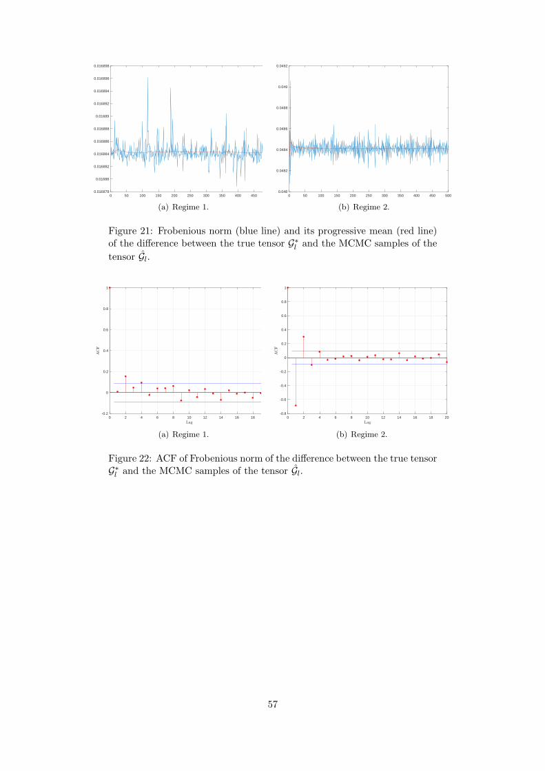
0 50 100 150 200 250 300 350 400 450 5000.016878

0.01688

0.016882

0.016884

0.016886

0.016888

0.01689

0.016892

0.016894

0.016896

0.016898

(a) Regime 1.

0 50 100 150 200 250 300 350 400 450 5000.048

0.0482

0.0484

0.0486

0.0488

0.049

0.0492

(b) Regime 2.

Figure 21: Frobenious norm (blue line) and its progressive mean (red line)of the difference between the true tensor G∗

l and the MCMC samples of the

tensor Gl.

0 2 4 6 8 10 12 14 16 18 20-0.2

0

0.2

0.4

0.6

0.8

1

(a) Regime 1.

0 2 4 6 8 10 12 14 16 18 20-0.8

-0.6

-0.4

-0.2

0

0.2

0.4

0.6

0.8

1

(b) Regime 2.

Figure 22: ACF of Frobenious norm of the difference between the true tensorG∗l and the MCMC samples of the tensor Gl.

57

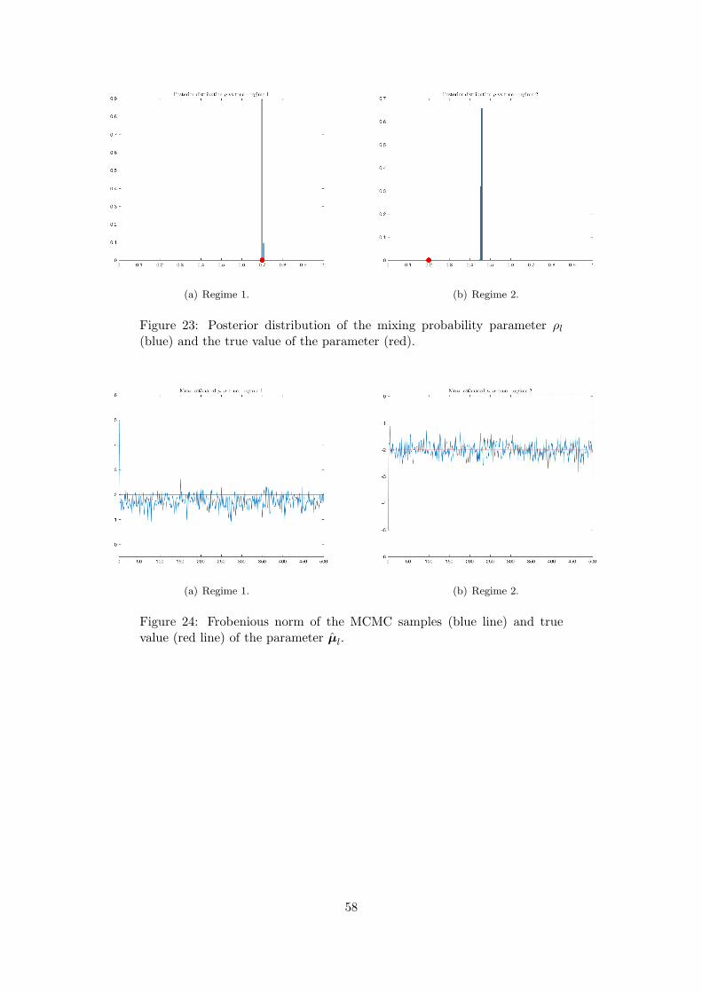
(a) Regime 1. (b) Regime 2.

Figure 23: Posterior distribution of the mixing probability parameter ρl(blue) and the true value of the parameter (red).

(a) Regime 1. (b) Regime 2.

Figure 24: Frobenious norm of the MCMC samples (blue line) and truevalue (red line) of the parameter µl.

58

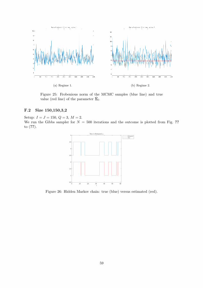
(a) Regime 1. (b) Regime 2.

Figure 25: Frobenious norm of the MCMC samples (blue line) and truevalue (red line) of the parameter Σl.

F.2 Size 150,150,3,2

Setup: I = J = 150, Q = 3, M = 2.We run the Gibbs sampler for N = 500 iterations and the outcome is plotted from Fig. ??to (??).

0 10 20 30 40 50 600.5

1

1.5

2

2.5

3

3.5

4

Figure 26: Hidden Markov chain: true (blue) versus estimated (red).

59

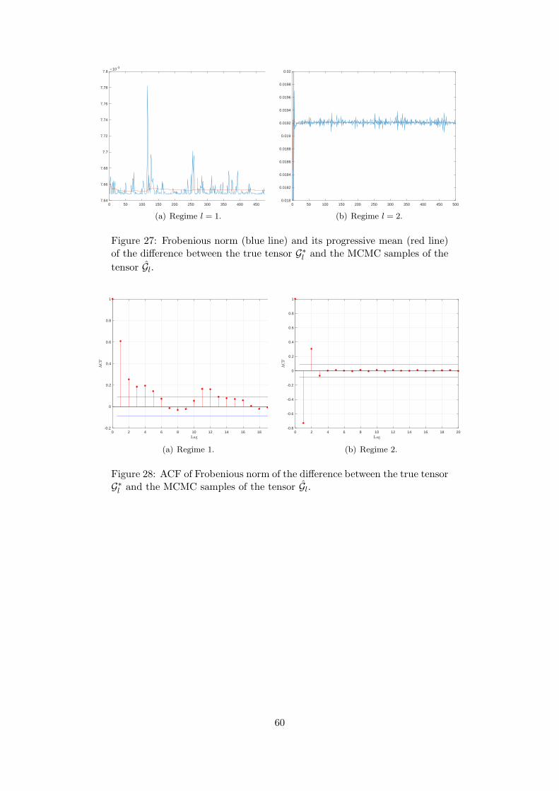
0 50 100 150 200 250 300 350 400 450 5007.64

7.66

7.68

7.7

7.72

7.74

7.76

7.78

7.810 -3

(a) Regime l = 1.

0 50 100 150 200 250 300 350 400 450 5000.018

0.0182

0.0184

0.0186

0.0188

0.019

0.0192

0.0194

0.0196

0.0198

0.02

(b) Regime l = 2.

Figure 27: Frobenious norm (blue line) and its progressive mean (red line)of the difference between the true tensor G∗

l and the MCMC samples of the

tensor Gl.

0 2 4 6 8 10 12 14 16 18 20-0.2

0

0.2

0.4

0.6

0.8

1

(a) Regime 1.

0 2 4 6 8 10 12 14 16 18 20-0.8

-0.6

-0.4

-0.2

0

0.2

0.4

0.6

0.8

1

(b) Regime 2.

Figure 28: ACF of Frobenious norm of the difference between the true tensorG∗l and the MCMC samples of the tensor Gl.

60

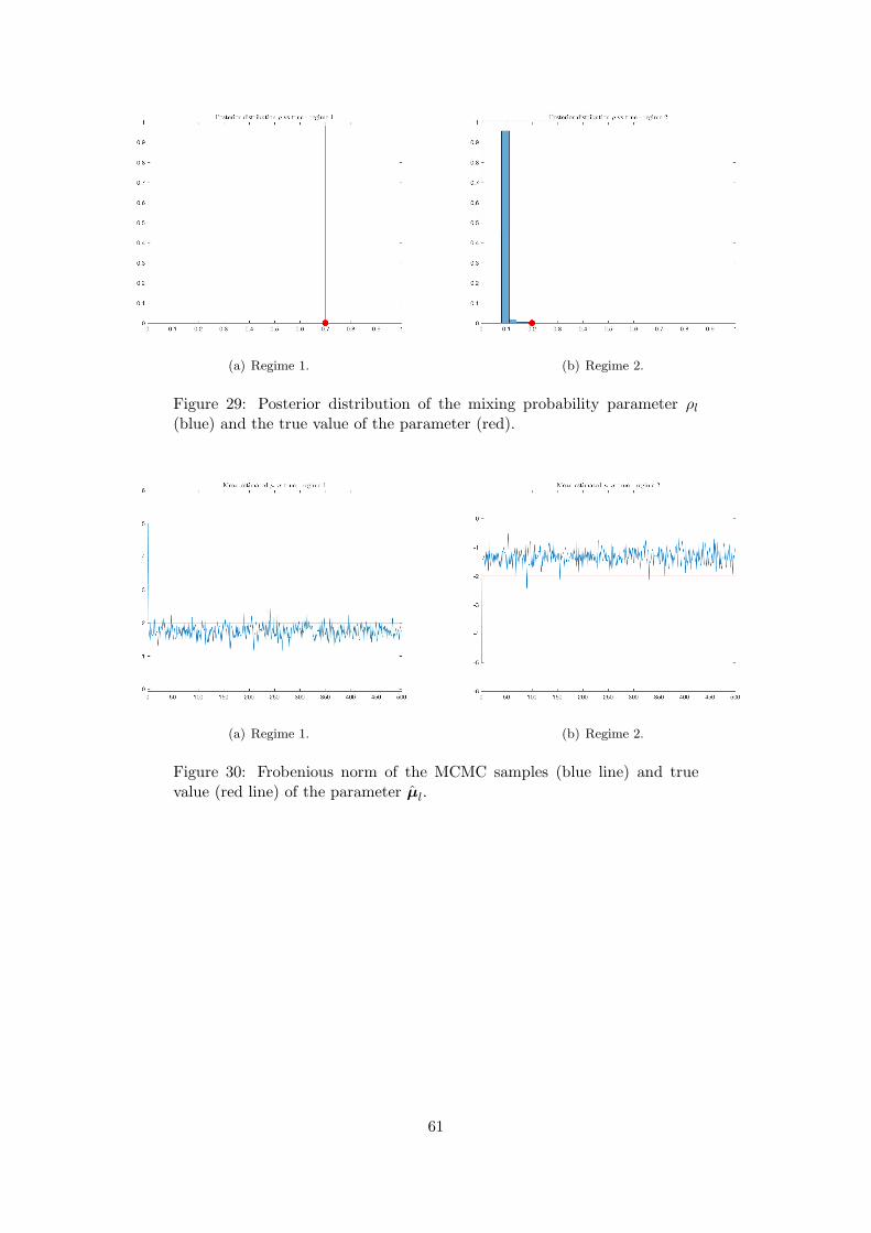
(a) Regime 1. (b) Regime 2.

Figure 29: Posterior distribution of the mixing probability parameter ρl(blue) and the true value of the parameter (red).

(a) Regime 1. (b) Regime 2.

Figure 30: Frobenious norm of the MCMC samples (blue line) and truevalue (red line) of the parameter µl.

61

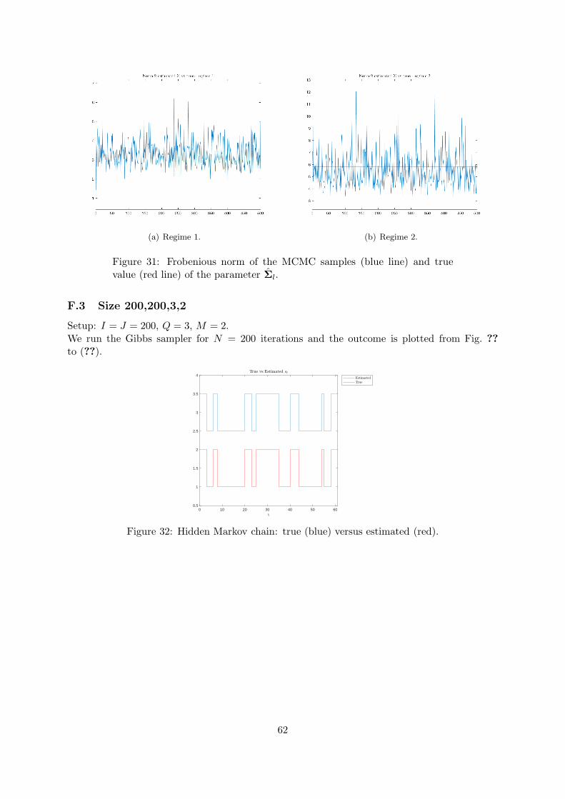
(a) Regime 1. (b) Regime 2.

Figure 31: Frobenious norm of the MCMC samples (blue line) and truevalue (red line) of the parameter Σl.

F.3 Size 200,200,3,2

Setup: I = J = 200, Q = 3, M = 2.We run the Gibbs sampler for N = 200 iterations and the outcome is plotted from Fig. ??to (??).

0 10 20 30 40 50 600.5

1

1.5

2

2.5

3

3.5

4

Figure 32: Hidden Markov chain: true (blue) versus estimated (red).

62

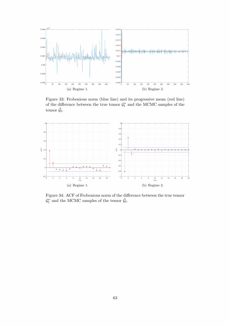
0 50 100 150 200 250 300 350 400 450 5006.2956

6.2958

6.296

6.2962

6.2964

6.2966

6.296810 -3

(a) Regime 1.

0 50 100 150 200 250 300 350 400 450 5000.0165

0.0166

0.0167

0.0168

0.0169

0.017

0.0171

0.0172

0.0173

0.0174

0.0175

(b) Regime 2.

Figure 33: Frobenious norm (blue line) and its progressive mean (red line)of the difference between the true tensor G∗

l and the MCMC samples of the

tensor Gl.

0 2 4 6 8 10 12 14 16 18 20-0.2

0

0.2

0.4

0.6

0.8

1

(a) Regime 1.

0 2 4 6 8 10 12 14 16 18 20-1

-0.8

-0.6

-0.4

-0.2

0

0.2

0.4

0.6

0.8

1

(b) Regime 2.

Figure 34: ACF of Frobenious norm of the difference between the true tensorG∗l and the MCMC samples of the tensor Gl.

63

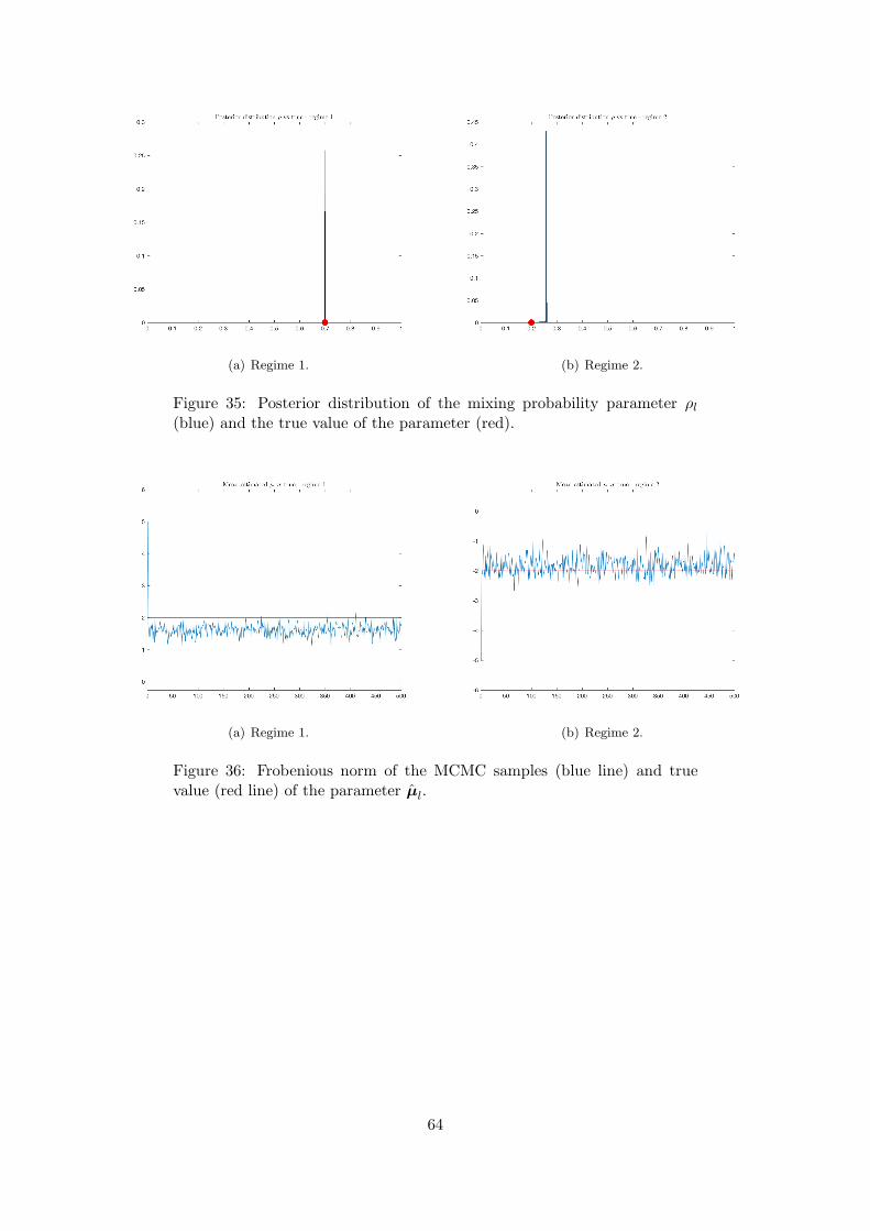
(a) Regime 1. (b) Regime 2.

Figure 35: Posterior distribution of the mixing probability parameter ρl(blue) and the true value of the parameter (red).

(a) Regime 1. (b) Regime 2.

Figure 36: Frobenious norm of the MCMC samples (blue line) and truevalue (red line) of the parameter µl.

64

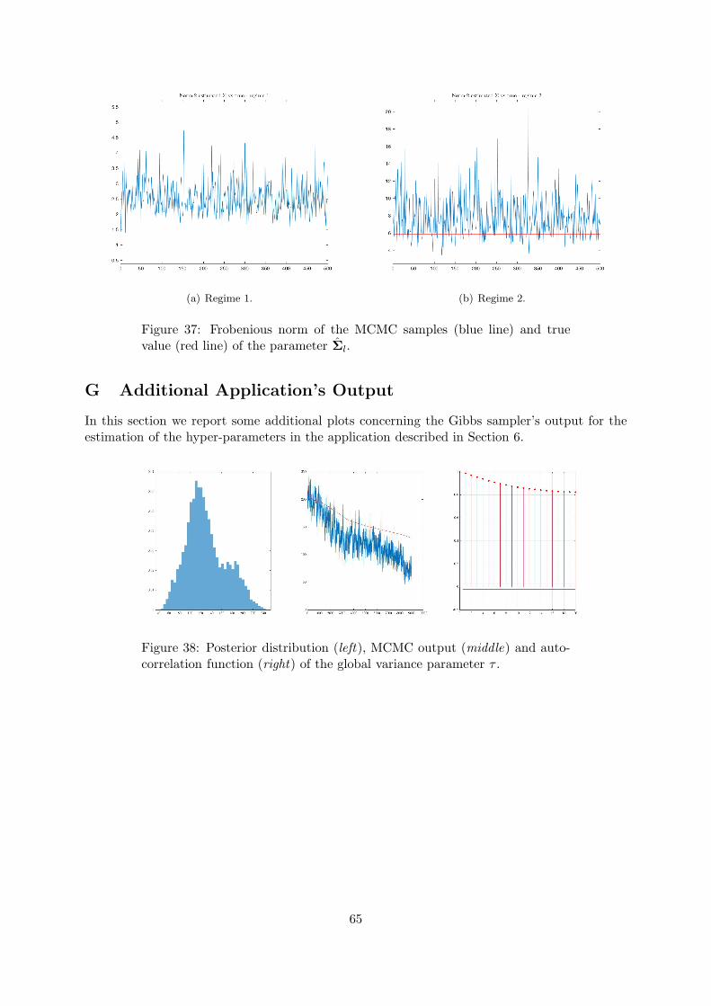
(a) Regime 1. (b) Regime 2.

Figure 37: Frobenious norm of the MCMC samples (blue line) and truevalue (red line) of the parameter Σl.

G Additional Application’s Output

In this section we report some additional plots concerning the Gibbs sampler’s output for theestimation of the hyper-parameters in the application described in Section 6.

Figure 38: Posterior distribution (left), MCMC output (middle) and auto-correlation function (right) of the global variance parameter τ .

65

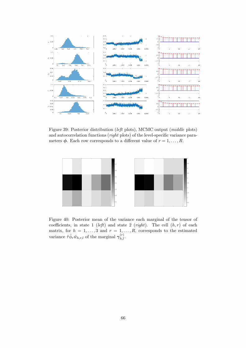
Figure 39: Posterior distribution (left plots), MCMC output (middle plots)and autocorrelation functions (right plots) of the level-specific variance para-meters φ. Each row corresponds to a different value of r = 1, . . . , R.

0.1

0.2

0.3

0.4

0.5

0.6

0.7

0.5

1

1.5

2

2.5

3

3.5

4

4.5

5

Figure 40: Posterior mean of the variance each marginal of the tensor ofcoefficients, in state 1 (left) and state 2 (right). The cell (h, r) of eachmatrix, for h = 1, . . . , 3 and r = 1, . . . , R, corresponds to the estimated

variance τ φrwh,r,l of the marginal γ(r)h,l .

66

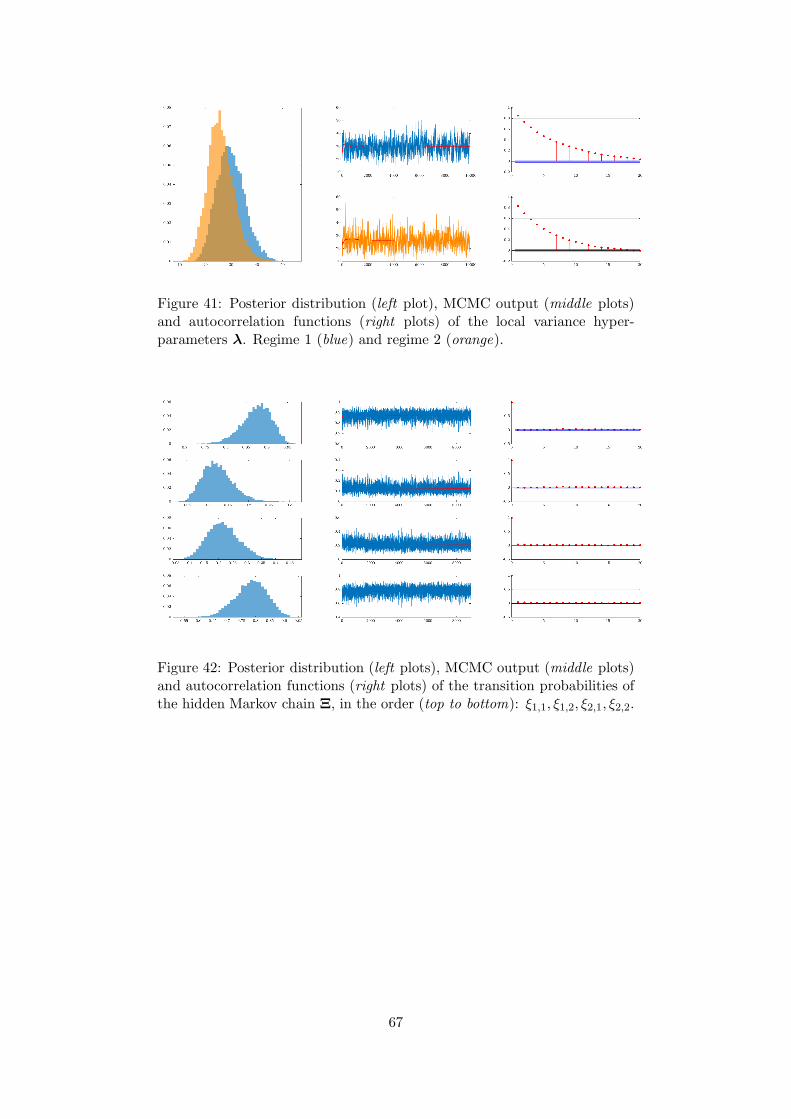
Figure 41: Posterior distribution (left plot), MCMC output (middle plots)and autocorrelation functions (right plots) of the local variance hyper-parameters λ. Regime 1 (blue) and regime 2 (orange).

Figure 42: Posterior distribution (left plots), MCMC output (middle plots)and autocorrelation functions (right plots) of the transition probabilities ofthe hidden Markov chain Ξ, in the order (top to bottom): ξ1,1, ξ1,2, ξ2,1, ξ2,2.

67

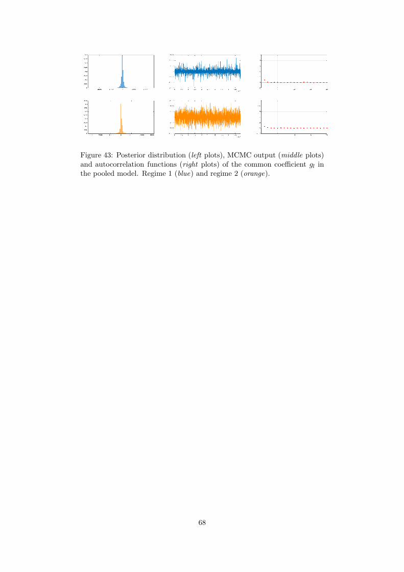
Figure 43: Posterior distribution (left plots), MCMC output (middle plots)and autocorrelation functions (right plots) of the common coefficient gl inthe pooled model. Regime 1 (blue) and regime 2 (orange).

68