NBER WORKING PAPER SERIES

BAYESIAN VARIABLE SELECTION FOR NOWCASTING ECONOMIC TIMESERIES

Steven L. ScottHal R. Varian

Working Paper 19567http://www.nber.org/papers/w19567

NATIONAL BUREAU OF ECONOMIC RESEARCH1050 Massachusetts Avenue

Cambridge, MA 02138October 2013

The views expressed herein are those of the authors and do not necessarily reflect the views of theNational Bureau of Economic Research.

NBER working papers are circulated for discussion and comment purposes. They have not been peer-reviewed or been subject to the review by the NBER Board of Directors that accompanies officialNBER publications.

© 2013 by Steven L. Scott and Hal R. Varian. All rights reserved. Short sections of text, not to exceedtwo paragraphs, may be quoted without explicit permission provided that full credit, including © notice,is given to the source.

Bayesian Variable Selection for Nowcasting Economic Time SeriesSteven L. Scott and Hal R. VarianNBER Working Paper No. 19567October 2013JEL No. C11,C53

ABSTRACT

We consider the problem of short-term time series forecasting (nowcasting) when there are more possiblepredictors than observations. Our approach combines three Bayesian techniques: Kalman filtering,spike-and-slab regression, and model averaging. We illustrate this approach using search engine querydata as predictors for consumer sentiment and gun sales.

Steven L. ScottGoogle1600 Amphitheatre ParkwayMountain View, CA 94043stevescott@google.com

Hal R. VarianGoogle1600 Amphitheatre ParkwayMountain View, CA 94043hal@sims.berkeley.edu

Bayesian Variable Selection for Nowcasting Economic

Time Series

Steven L. Scott

Hal R. Varian

July 2012

THIS DRAFT:August 21, 2013

Abstract

We consider the problem of short-term time series forecasting (nowcasting) when there

are more possible predictors than observations. Our approach combines three Bayesian

techniques: Kalman filtering, spike-and-slab regression, and model averaging. We

illustrate this approach using search engine query data as predictors for consumer

sentiment and gun sales.

1 Introduction

Computers are now in the middle of many economic transactions. The details of these

“computer mediated transactions” can be captured in databases and be used in subsequent

analyses (Varian [2010].) However such databases can contain vast amounts of data, so it is

normally necessary to do some sort of data reduction.

Our motivating examples for this work is Google Trends, a system that produces an

index of search activity on queries entered into Google. A related system, Google Correlate,

produces an index of queries that are correlated with a time series entered by user. There

are many uses for these data, but in this paper we focus on how to use the data to make

short run forecasts of economic metrics.

Choi and Varian [2009a,b, 2011, 2012] described how to use search engine data to fore-

cast contemporaneous values of macroeconomic indicators. This type of contemporaneous

1

forecasting, or “nowcasting,” is of particular interest to central banks, and there have been

several subsequent research studies from researches at these institutions. See, for example,

Arola and Galan [2012], McLaren and Shanbhoge [2011], Hellerstein and Middeldorp [2012],

Suhoy [2009], Carriere-Swallow and Labbe [2011]. Choi and Varian [2012] contains several

other references to work in this area. Wu and Brynjolfsson [2009] describe an application of

Trends data to the real estate market using cross-state data.

In these studies, the researchers selected predictors using their judgment of relevance to

the particular prediction problem. For example, it seems natural that search engine queries

in the “Vehicle Shopping” category would be good candidates for forecasting automobile

sales while queries such as “file for unemployment” would be useful in forecasting initial

claims for unemployment benefits.

One difficulty with using human judgment is that it does not easily scale to models

where the number of possible predictors exceeds the number of observations—the so-called

“fat regression” problem. For example, the Google Trend service provides data for millions

of search queries and hundreds of search categories extending back to January 1, 2004. Even

if we restrict ourselves to using only categories of queries, we will have several hundred

possible possible predictors for about 100 months of data. In this paper we describe a

scalable approach to time series prediction for fat regressions of this sort.

2 Approaches to variable selection

Castle et al. [2009, 2010] describes and compares 21 techniques for variable selection for

time-series forecasting. These techniques fall into 4 major categories.

• Significance testing (forward and backward stepwise regression, Gets )

• Information criteria (AIC, BIC)

• Principle component and factor models (e.g. Stock and Watson [2010])

• Lasso, ridge regression and other penalized regression models (e.g., Hastie et al. [2009])

Our approach combines three statistical methods into an integrated system we call

Bayesian Structural Time Series or BSTS for short.

• A “basic structural model” for trend and seasonality, estimated using Kalman filters;

• Spike and slab regression for variable selection;

2

• Bayesian model averaging over the best performing models for the final forecast.

We briefly review each of these methods and how they fit into our framework.

2.1 Structural time series and the Kalman filter

Harvey [1991], Durbin and Koopman [2001], Petris et al. [2009] and many others have ad-

vocated the use of Kalman filters for time series forecasting. The “basic structural model”

decomposes the time series into four components: a level, a local trend, seasonal effects and

an error term. The model described here drops the seasonal effect for simplicity and adds a

regression component; it called a “local linear trend model with regressors.”

This model is a stochastic generalization of the classic constant-trend regression model,

yt = µ+ bt+ βxt + et

In this classic model the level (µ) and trend (b) parameters are constant, (xt) is a vector of

contemporaneous regressors, β is a vector of regression coefficients, and et is an error term.

In local linear trend model each of these structural components is stochastic. In partic-

ular, the level and slope terms each follow a random walk model.

yt = µt + zt + vt vt ∼ N(0, V ) (1)

µt = µt−1 + bt−1 + w1t w1t ∼ N(0,W1) (2)

bt = bt−1 + w2t w2t ∼ N(0,W2) (3)

zt = βxt (4)

The unknown parameters to be estimated in this system are the variance terms (V,W1,W2)

and the regression coefficients, β.

If we drop the trend and regression coefficients by setting bt = 0 and β = 0, the “local

trend model” becomes the “local level” model. When V = 0, the local level model is a

random walk, so the best forecast of yt+1 is yt. When W1 = 0, the local level model is a

constant mean model, so the best forecast of yt+1 is the average of all previously observed

values of yt. Hence, this model yields two popular time series models as special cases.

It is easy to add a seasonal component to the local linear trend model, in which case it is

referred to as the “basic structural model.” In the Appendix we describe a general structural

time series model that contains these and other models in the literature as special cases.

3

It is also possible to allow for time-varying regression coefficients by simply including

them as another set of state variables. In practice, one would want to limit this to just a few

coefficients, particularly when dealing with sample sizes common in economic applications.

2.2 Spike and slab variable selection

The spike-and-slab approach to model selection was developed by George and McCulloch

[1997a]) and Madigan and Raftery [1994].

Let γ denote a vector the same length as the list of possible regressors that indicates

where or not a particular regressor is included in the regression. More precisely, γ is a vector

the same length as β, where γi = 1 indicates βi 6= 0 and γi = 0 indicates βi = 0. Let

βγ indicate the subset of β for which γi = 1, and let σ2 be the residual variance from the

regression model.

A spike and slab prior for the joint distribution of (β, γ, σ−2) can be factored in the usual

way.

p(β, γ, σ−2) = p(βγ|γ, σ−2)p(σ−2|γ)p(γ). (5)

There are several ways to specify functional forms for these prior distributions. Here we

describe a particularly convenient choice.

The “spike” part of a spike-and-slab prior refers to the point mass at zero, for which we

assume a Bernoulli distribution for each i, so that the prior is a product of Bernoullis:

γ ∼∏i

πγii (1− πi)1−γi . (6)

When detailed prior information is unavailable, it is convenient to set all πi equal to the same

number, π. The common prior inclusion probability can easily be elicited from the expected

number of nonzero coefficients. If k out of K coefficients are expected to be nonzero then

set π = k/K in the prior.

More complex choices of p(γ) can be made as well. For example, a non-Bernoulli model

could be used to encode rules such as the hierarchical principle (no high order interactions

without lower order interactions). The MCMC methods described below are robust to the

specific choice of the prior.

The “slab” component is a prior for the values of the nonzero coefficients, conditional on

knowledge of which coefficients are nonzero. Let b be a vector of prior guesses for regression

coefficients, let Ω−1 be a prior precision matrix, and let Ω−1γ denote rows and columns of Ω−1

4

for which γi = 1. A conditionally conjugate “slab” prior is

βγ|γ, σ2 ∼ N(bγ, σ

2(Ω−1γ

)−1),

1

σ2∼ Γ

(df

2,ss

2

).

(7)

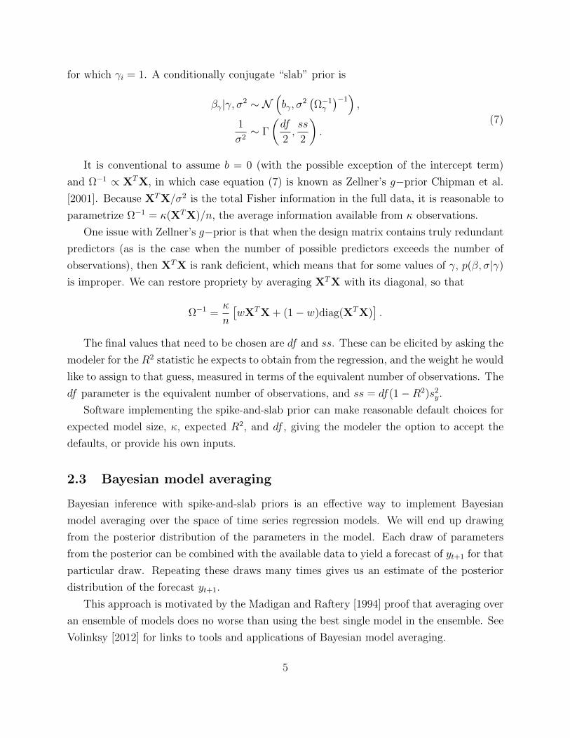
It is conventional to assume b = 0 (with the possible exception of the intercept term)

and Ω−1 ∝ XTX, in which case equation (7) is known as Zellner’s g−prior Chipman et al.

[2001]. Because XTX/σ2 is the total Fisher information in the full data, it is reasonable to

parametrize Ω−1 = κ(XTX)/n, the average information available from κ observations.

One issue with Zellner’s g−prior is that when the design matrix contains truly redundant

predictors (as is the case when the number of possible predictors exceeds the number of

observations), then XTX is rank deficient, which means that for some values of γ, p(β, σ|γ)

is improper. We can restore propriety by averaging XTX with its diagonal, so that

Ω−1 =κ

n

[wXTX + (1− w)diag(XTX)

].

The final values that need to be chosen are df and ss. These can be elicited by asking the

modeler for the R2 statistic he expects to obtain from the regression, and the weight he would

like to assign to that guess, measured in terms of the equivalent number of observations. The

df parameter is the equivalent number of observations, and ss = df(1−R2)s2y.

Software implementing the spike-and-slab prior can make reasonable default choices for

expected model size, κ, expected R2, and df , giving the modeler the option to accept the

defaults, or provide his own inputs.

2.3 Bayesian model averaging

Bayesian inference with spike-and-slab priors is an effective way to implement Bayesian

model averaging over the space of time series regression models. We will end up drawing

from the posterior distribution of the parameters in the model. Each draw of parameters

from the posterior can be combined with the available data to yield a forecast of yt+1 for that

particular draw. Repeating these draws many times gives us an estimate of the posterior

distribution of the forecast yt+1.

This approach is motivated by the Madigan and Raftery [1994] proof that averaging over

an ensemble of models does no worse than using the best single model in the ensemble. See

Volinksy [2012] for links to tools and applications of Bayesian model averaging.

5

3 Estimating the model

The Kalman filter, spike-and-slab regression, and model averaging all have natural Bayesian

interpretations and tend to play well together. The basic parameters we need to estimate are

γ (which variables are in the regression), β (the regression coefficients), and the variances of

the error terms (V,W1,W2,W3).

As the appendix describes in detail, we specify priors for each of these parameters and

then sample from the posterior distribution using Markov Chain Monte Carlo techniques.

There are a number of attractive short cuts available that make this sampling process quite

efficient. These are described in more detail in the appendix and in a companion paper,

Scott and Varian [2012].

These techniques yield a sample from the posterior distribution for the parameters that

can be then used to construct a posterior distribution for forecasts of time series of interest.

4 Fun with priors

We have already indicated that it is possible to use an informative prior to describe beliefs

about the expected number of predictors. It is also possible to use a prior in the regression

to indicate likely relationships. For example, one might expect that autmobile purchases are

likely to be correlated with automotive-related queries.

A less obvious example involves using data-based priors for estimating the state and

observation variances, (V,W1,W2,W3). Even though the Google Trends data only goes back

to 2004, economic time series are often much longer. One can estimate posterior distribution

the parameters in the univariate Kalman filter using the long series, then use this posterior

distribution as the prior distribution for the shorter series where the Google Trends data are

available.

5 Nowcasting consumer sentiment

To illustrate the use of BSTS for nowcasting, we use the University of Michigan monthly

survey of Consumer Sentiment from January 2004-April 2012. We focus on “nowcasting”

since we expect that queries at time t could be related to sentiment at time t but are not

necessarily predictive of future sentiment.

Our data from Google Trends starts at January 2004, and our sample ends in April

6

2012, giving us 100 observations. For predictors, we use 151 categories from Google Trends

that have some connection with economics. These potential predictors were chosen from the

roughly 300 query categories using the authors’ judgment.

Our problem is to find a good set of predictors for 100 observations chosen from a set of

151 possible predictors. This qualifies as a mildly obese, if not actually fat, regression.

The Consumer Sentiment index is not highly seasonal but many of the potential predictors

are seasonal so we first deseasonalize the data by using the R command stl. We then detrend

the predictors by regressing each predictor on a simple time trend. A visual inspection of

the time series of the predictors indicated that these techniques were sufficient to “whiten”

the data.

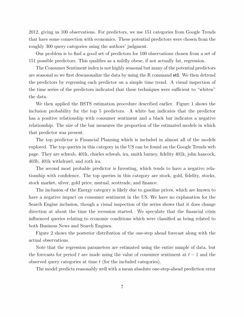
We then applied the BSTS estimation procedure described earlier. Figure 1 shows the

inclusion probability for the top 5 predictors. A white bar indicates that the predictor

has a positive relationship with consumer sentiment and a black bar indicates a negative

relationship. The size of the bar measures the proportion of the estimated models in which

that predictor was present.

The top predictor is Financial Planning which is included in almost all of the models

explored. The top queries in this category in the US can be found on the Google Trends web

page. They are schwab, 401k, charles schwab, ira, smith barney, fidelity 401k, john hancock,

403b, 401k withdrawl, and roth ira.

The second most probable predictor is Investing, which tends to have a negative rela-

tionship with confidence. The top queries in this category are stock, gold, fidelity, stocks,

stock market, silver, gold price, mutual, scottrade, and finance.

The inclusion of the Energy category is likely due to gasoline prices, which are known to

have a negative impact on consumer sentiment in the US. We have no explanation for the

Search Engine inclusion, though a visual inspection of the series shows that it does change

direction at about the time the recession started. We speculate that the financial crisis

influenced queries relating to economic conditions which were classified as being related to

both Business News and Search Engines.

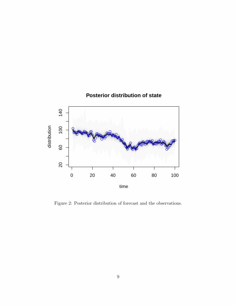
Figure 2 shows the posterior distribution of the one-step ahead forecast along with the

actual observations.

Note that the regression parameters are estimated using the entire sample of data, but

the forecasts for period t are made using the value of consumer sentiment at t − 1 and the

observed query categories at time t (for the included categories).

The model predicts reasonably well with a mean absolute one-step-ahead prediction error

7

Energy.Utilities

Search.Engines

Business.News

Investing

Financial.Planning

Inclusion Probability

0.0 0.2 0.4 0.6 0.8 1.0

Figure 1: Top 5 predictors for consumer sentiment. Bars show the probability of inclusion.Shading indicates the sign of the coefficient.

8

time

dist

ribut

ion

0 20 40 60 80 100

2060

100

140

Posterior distribution of state

Figure 2: Posterior distribution of forecast and the observations.

9

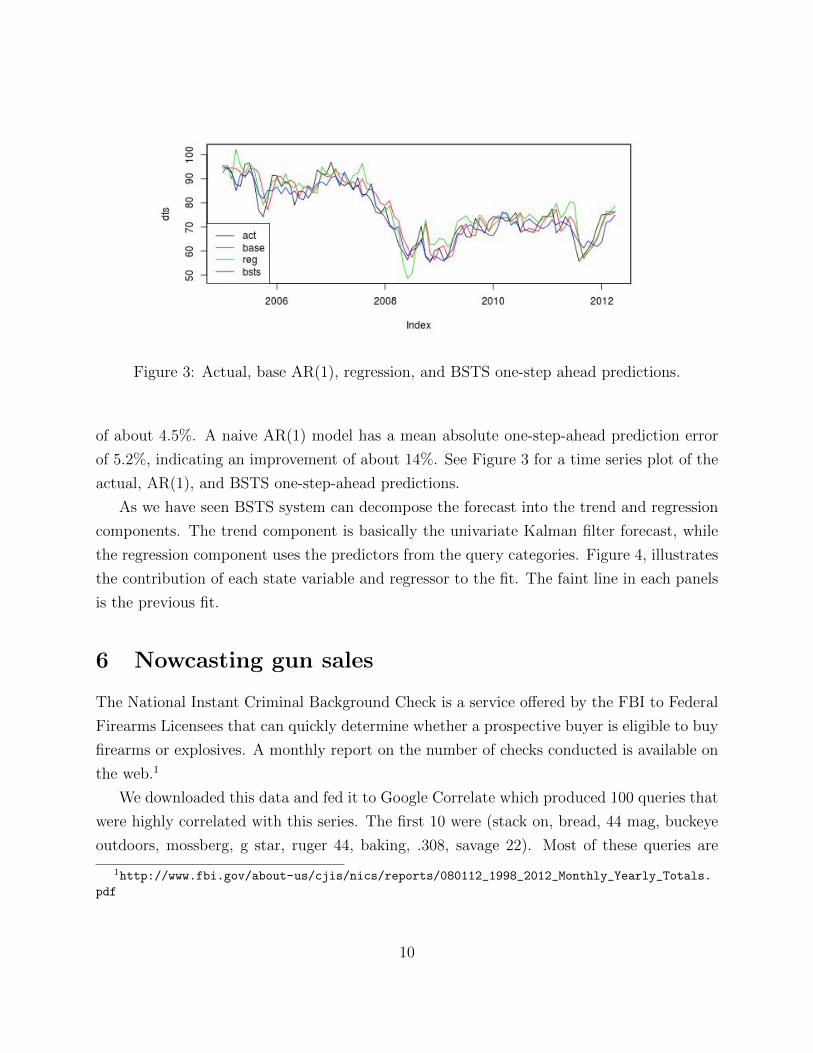
Figure 3: Actual, base AR(1), regression, and BSTS one-step ahead predictions.

of about 4.5%. A naive AR(1) model has a mean absolute one-step-ahead prediction error

of 5.2%, indicating an improvement of about 14%. See Figure 3 for a time series plot of the

actual, AR(1), and BSTS one-step-ahead predictions.

As we have seen BSTS system can decompose the forecast into the trend and regression

components. The trend component is basically the univariate Kalman filter forecast, while

the regression component uses the predictors from the query categories. Figure 4, illustrates

the contribution of each state variable and regressor to the fit. The faint line in each panels

is the previous fit.

6 Nowcasting gun sales

The National Instant Criminal Background Check is a service offered by the FBI to Federal

Firearms Licensees that can quickly determine whether a prospective buyer is eligible to buy

firearms or explosives. A monthly report on the number of checks conducted is available on

the web.1

We downloaded this data and fed it to Google Correlate which produced 100 queries that

were highly correlated with this series. The first 10 were (stack on, bread, 44 mag, buckeye

outdoors, mossberg, g star, ruger 44, baking, .308, savage 22). Most of these queries are

1http://www.fbi.gov/about-us/cjis/nics/reports/080112_1998_2012_Monthly_Yearly_Totals.

pdf

10

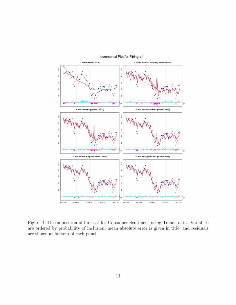
Figure 4: Decomposition of forecast for Consumer Sentiment using Trends data. Variablesare ordered by probability of inclusion, mean absolute error is given in title, and residualsare shown at bottom of each panel.

11

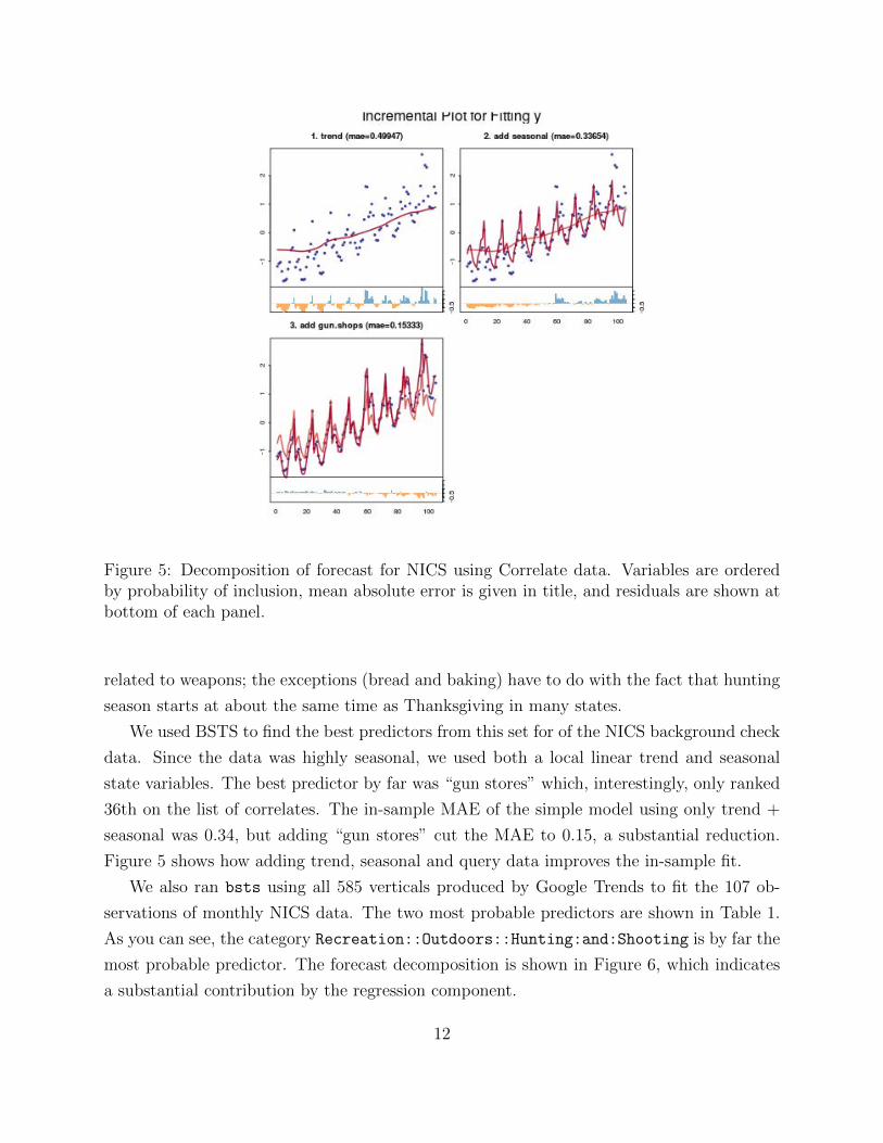
Figure 5: Decomposition of forecast for NICS using Correlate data. Variables are orderedby probability of inclusion, mean absolute error is given in title, and residuals are shown atbottom of each panel.

related to weapons; the exceptions (bread and baking) have to do with the fact that hunting

season starts at about the same time as Thanksgiving in many states.

We used BSTS to find the best predictors from this set for of the NICS background check

data. Since the data was highly seasonal, we used both a local linear trend and seasonal

state variables. The best predictor by far was “gun stores” which, interestingly, only ranked

36th on the list of correlates. The in-sample MAE of the simple model using only trend +

seasonal was 0.34, but adding “gun stores” cut the MAE to 0.15, a substantial reduction.

Figure 5 shows how adding trend, seasonal and query data improves the in-sample fit.

We also ran bsts using all 585 verticals produced by Google Trends to fit the 107 ob-

servations of monthly NICS data. The two most probable predictors are shown in Table 1.

As you can see, the category Recreation::Outdoors::Hunting:and:Shooting is by far the

most probable predictor. The forecast decomposition is shown in Figure 6, which indicates

a substantial contribution by the regression component.

12

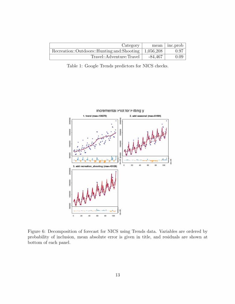
Category mean inc.probRecreation::Outdoors::Hunting:and:Shooting 1,056,208 0.97

Travel::Adventure:Travel -84,467 0.09

Table 1: Google Trends predictors for NICS checks.

Figure 6: Decomposition of forecast for NICS using Trends data. Variables are ordered byprobability of inclusion, mean absolute error is given in title, and residuals are shown atbottom of each panel.

13

7 Conclusion

We have described a Bayesian approach to variable selection for time series that combines

Kalman filtering, spike and slab regressions, and model averaging. Although the system

was developed for nowcasting using Google Trends data, there are many other possible

applications.

We have focused on nowcasting since in most cases the action taken by individuals is

contemporaneous with the related queries. But in some cases, such as vacation planning or

housing purchases, the relevant queries may precede the actions by several months. In such

cases queries may help in longer-term forecasting. (See, e.g., Choi and Liu [2011].)

As more and more data becomes available the problem of “fat regressions” will arise in

many other contexts. We hope that Bayesian Structural Time Series may well be helpful in

those cases.

8 Appendices

A Structural time series models

Here we describe our Bayesian Structural Time Series model. More detail can be found in

Scott and Varian [2012]. We focus on structural time series models of the standard form

yt = ZTt αt + εt εt ∼ N (0, Ht)

αt+1 = Ttαt +Rtηt ηt ∼ N (0, Qt) .(8)

Here yt is time series to be modeled and the vector αt is a latent variable indicating the

state of the model; it contains any trend, seasonal, or other components deemed necessary

by the modeler.

Zt is a vector of coefficients applied to the state variables, εt is a Normally distributed

error term with mean zero and Ht is its variance. Each state component contributes to the

block diagonal transition matrix Tt, the rectangular block diagonal residual matrix Rt, and

the observation vector Zt. The error term ηt has covariance matrix Qt.

The model matrices (Z, T,R,H,Q) can be used to construct the Kalman filter, which

can then be used to forecast future values yt+τ from current observations (y1, . . . , yt). One

attractive feature of the Kalman filter is that it has a natural Bayesian interpretation and

can easily be combined with the variable selection and model averaging techniques we have

14

chosen.

A.1 Regression

Regressors can be included in a structural time series model in either a static framework

(where the regression coefficients are fixed) or dynamic framework (where the regression

coefficients can change over time).

In a dynamic regression the coefficients are a component of the state vector which evolve

over time according to some stochastic process. In a static regression, by contrast, the

coefficients are fixed, unknown parameters. A convenient way to include a static regression

component in the model is to set αt = 1, tt = 1, qt = 0, and zt = βtxt. This specification

adds βtxt to the contributions of the other state components in a computationally efficient

way, because it only adds one additional state to the model. A small dimension is helpful

because the Kalman recursions are quadratic in the dimension of the state space.

B Estimating the model using Markov Chain Monte

Carlo

We estimate the posterior distribution of the model parameters using Markov Chain Monte

Carlo. Let θ denote the collection of model parameters (β, σ, ψ) where ψ is the collection

of all model parameters associated with state components other than the static regression.

Then the complete data posterior distribution is

p(θ,α|y) ∝ p(θ)p(α0)n∏t=1

p(yt|αt, θ)p(αt|αt−1, θ). (9)

In order to sample from the posterior distribution we use an efficient Gibbs sampling al-

gorithm that alternates between draws of p(α|θ,y) and p(θ|α,y), which produces a sequence

(θ,α)0, (θ,α)1, . . . from a Markov chain with stationary distribution p(θ,α|y).

The key point is that, conditional on α, the time series and regression components of the

model are independent. Thus the draw from p(θ|α,y) decomposes into several independent

draws from the different conditional posterior distributions of the state components. In

particular, p(ψ, β, σ−2|α,y) = p(ψ|α,y)p(β, σ−2|α,y).

15

B.1 Sampling α

The idea of using Kalman filtering to sample the state in a linear Gaussian structural

time series model was independently proposed by [Carter and Kohn, 1994] and [Fruhwirth-

Schnatter, 1994]. Various improvements to the early algorithms have been made by [de Jong

and Shepard, 1995] [Rue, 2001], and others. We use the method proposed by [Durbin and

Koopman, 2002], who observed that the variance of p(α|θ,y) does not depend on the nu-

merical value of y. Durbin and Koopman [2001] describes a fast smoothing method for

computing E(α|y, θ) using the Kalman filter.

Thus one may simulate a fake data set (y∗,α∗) ∼ p(y,α|θ) by simply iterating equa-

tion (8). Then the fast mean smoother can be used to subtract the conditional mean

E(α∗|θ,y∗) from α∗, which is now mean zero with the correct variance. A second fast

smoother can be used to add in E(α|y, θ), yielding a draw of α with the correct moments.

Because p(α|y, θ) is Gaussian, the correct moments imply the correct distribution.

B.2 Sampling θ

Many of the usual models for state components are simple random walks, whose variance

parameters are trivial to sample conditional on α. For example, consider the state variables

for the local linear trend model described in 4

µt+1 = µt + δt + η0t

δt+1 = δt + η1t,

where η0 and η1 are independent Gaussian error terms with variances ψ20 and ψ2

1. With

independent Gamma priors on ψ−20 ∼ Γ(df0/2, ss0/2) and ψ−21 ∼ Γ(df1/2, ss1/2), their full

conditional is the product of two independent Gamma distributions

p(ψ−20 , ψ21|α) = Γ

(df0 + n− 1

2,SS0

2

)Γ

(df1 + n− 1

2,SS1

2

),

where SS0 = ss0 +∑n

t=2(µt − µt−1 − δt−1)2 and SS1 = ss1 +

∑nt=2(δt − δt−1)

2. These

complete data sufficient statistics are observed given α, so drawing ψ−20 and ψ−21 from their

full conditional distribution is trivial. Most of the traditional state models can be handled

similarly, including the seasonal component of the BSM and dynamic regression coefficients.

The full conditional for (β, σ−2) is likewise independent of the other state components,

with yt = yt − ZTt αt + βTxt ∼ N

(βTxt, σ

2). Thus, by subtracting the contributions from

16

the other state components from each yt we are left with a standard spike and slab regres-

sion. The posterior distribution can be simulated efficiently by drawing from p(γ|α,y) using

a sequence of Gibbs sampling steps, and then drawing from the well known closed form

p(βγ, σ−2|γ,α,y). This technique is known as “stochastic search variable selection” [George

and McCulloch, 1997b]. There have been many suggested improvements to the SSVS algo-

rithm (notably [Ghosh and Clyde, 2011]), but we have obtained satisfactory results with the

basic algorithm.

The conditional posteriors for βγ and σ−2 can be found in standard texts [e.g. Gelman

et al., 2002]. They are

p(β|y,α, γ, σ−2) = N(βγ, σ

2Vγ

), and

p(σ−2|y,α, γ) = Γ

(df + n

2,ss+ S

2

),

(10)

where the complete data sufficient statistics are V −1γ = XTXγ+Ω−1γ , βγ = Vγ(XT yγ+Ω−1γ bγ),

and S =∑n

t=1(yt − xTt βγ)2 + (βγ − bγ)TΩ−1γ (βγ − bγ). The distribution for p(γ|α,y) can be

shown to be

p(γ|y,α) ∝|Ω−1γ |−1/2

|V −1γ |−1/2S−(df+n)/2. (11)

Let |γ| denote the number of included components. Under Zellner’s g−prior it is easy to see

that|Ω−1γ ||Vγ|

=

(κ/n

1 + κ/n

)|γ|is decreasing in |γ|. It is true in general that |Ω−1γ | ≤ |Ω−1γ + XTXγ| which implies that

p(γ|y,α) prefers models with few predictors and small residual variation.

Equation (11) can be used in a Gibbs sampling algorithm that draws each γi given

γ−i (the elements of γ other than γi). Each full conditional distribution is proportional

to equation (11), and γi can only assume two possible values. Notice that p(γ|y,α) only

requires matrix computations for those variables that are actually included in the model.

Thus if the model is sparse the Gibbs sampler involves many inexpensive decompositions

of small matrices, which makes SSVS computationally tractable even for problems with a

relatively large number of predictors.

17

References

Concha Arola and Enrique Galan. Tracking the future on the web: Con-

struction of leading indicators using internet searches. Technical report, Bank

of Spain, 2012. URL http://www.bde.es/webbde/SES/Secciones/Publicaciones/

PublicacionesSeriadas/DocumentosOcasionales/12/Fich/do1203e.pdf.

Yan Carriere-Swallow and Felipe Labbe. Nowcasting with google trends in an emerging

market. Journal of Forecasting, 2011. doi: 10.1002/for.1252. URL http://ideas.repec.

org/p/chb/bcchwp/588.html. Working Papers Central Bank of Chile 588.

Chris K. Carter and Robert Kohn. On Gibbs sampling for state space models. Biometrika,

81(3):541–553, 1994.

Jennifer L. Castle, Xiaochuan Qin, and W. Robert Reed. How to pick the best regression

equation: A review and comparison of model selection algorithms. Technical Report

13/2009, Department of Economics, University of Canterbury, 2009. URL http://www.

econ.canterbury.ac.nz/RePEc/cbt/econwp/0913.pdf.

Jennifer L. Castle, Nicholas W. P. Fawcett, and David F. Hendry. Evaluating automatic

model selection. Technical Report 474, Department of Economics, University of Oxford,

2010. URL http://economics.ouls.ox.ac.uk/14734/1/paper474.pdf.

Hugh Chipman, Edward I. George, Robert E. McCulloch, Merlise Clyde, Dean P. Foster,

and Rober A. Stine. The practical implementation of Bayesian model selection. Lecture

Notes-Monograph Series, pages 65–134, 2001.

Hyunyoung Choi and Paul Liu. Reading tea leaves in the tourism industry:

a case study in the Gulf oil spill. Technical report, Google, 2011. URL

http://www.google.com/url?q=http%3A%2F%2Fwww.google.com%2Fgoogleblogs%

2Fpdfs%2Fgoogle_gulf_tourism_march2011.pdf.

Hyunyoung Choi and Hal Varian. Predicting the present with Google Trends. Tech-

nical report, Google, 2009a. URL http://google.com/googleblogs/pdfs/google_

predicting_the_present.pdf.

Hyunyoung Choi and Hal Varian. Predicting initial claims for unemployment insurance using

Google Trends. Technical report, Google, 2009b. URL http://research.google.com/

archive/papers/initialclaimsUS.pdf.

18

Hyunyoung Choi and Hal Varian. Using search engine data for nowcasting—

an illustration. In Actes des Rencontrees Economiques, pages 535–538, Aix-en-

Provence, FRANCE, 2011. Recontres Economiques d′Aix-en-Provence, Le Cercle des

economistes. URL http://www.lecercledeseconomistes.asso.fr/IMG/pdf/Actes_

Rencontres_Economiques_d_Aix-en-Provence_2011.pdf.

Hyunyoung Choi and Hal Varian. Predicting the present with google trends. Economic

Record, 2012. URL http://people.ischool.berkeley.edu/~hal/Papers/2011/ptp.

pdf. Forthcoming.

Piet de Jong and Neil Shepard. The simulation smoother for time series models. Biometrika,

82(2):339–350, 1995.

J. Durbin and S. J. Koopman. A simple and efficient simulation smoother for state space

time series analysis. Biometrika, 89(3):603–616, 2002.

James Durbin and Siem Jan Koopman. Time Series Analysis by State Space Methods. Oxford

University Press, 2001.

Sylvia Fruhwirth-Schnatter. Data augmentation and dynamic linear models. Journal of

Time Series Analysis, 15(2):183–202, 1994.

Andrew Gelman, John B. Carlin, Hal S. Stern, and Donald B. Rubin. Bayesian Data Analysis

(2nd ed). Chapman & Hall, 2002.

Edward I. George and Robert E. McCulloch. Approaches for Bayesian variable selection. Sta-

tistica Sinica, 7:339–373, 1997a. URL http://www3.stat.sinica.edu.tw/statistica/

oldpdf/A7n26.pdf.

Edward I. George and Robert E. McCulloch. Approaches for Bayesian variable selection.

Statistica Sinica, 7:339–374, 1997b.

Joyee Ghosh and Merlise A. Clyde. Rao-Blackwellization for Bayesian variable selection and

model averaging in linear and binary regression: A novel data augmentation approach.

Journal of the American Statistical Association, 106(495):1041–1052, 2011.

Andrew Harvey. Forecasting, Structural Time Series Models and the Kalman Filter. Cam-

bridge University Press, 1991.

19

Trevor Hastie, Robert Tibshirani, and Jerome Friedman. The Elements of Statistical Learn-

ing. Springer, 2 edition, 2009.

Rebecca Hellerstein and Menno Middeldorp. Forecasting with internet search

data. Liberty Street Economics Blog of the Federal Reserve Bank of New York,

Jan 4 2012. URL http://libertystreeteconomics.newyorkfed.org/2012/01/

forecasting-with-internet-search-data.html.

David M. Madigan and Adrian E. Raftery. Model selection and accounting for model un-

certainty in graphical models using occam’s window. Journal of the American Statistical

Association, 89:1335–1346, 1994.

Nick McLaren and Rachana Shanbhoge. Using internet search data as economic indicators.

Bank of England Quarterly Bulletin, June 2011. URL http://www.bankofengland.co.

uk/publications/quarterlybulletin/qb110206.pdf.

Giovanni Petris, Sonia Petrone, and Patrizia Campagnoli. Dynamic Linar Models with R.

Springer, 2009.

Havard Rue. Fast sampling of Gaussian Markov random fields. Journal of the Royal Statis-

tical Society: Series B (Statistical Methodology), 63(2):325–338, 2001. ISSN 1467-9868.

Steven L. Scott and Hal R. Varian. Predicting the present with Bayesian structural time se-

ries. Technical report, Google, Inc., 2012. URL http://papers.ssrn.com/sol3/papers.

cfm?abstract_id=2304426. Presented at JSM 2012, San Diego. To appear in Interna-

tional Journal of Mathematical Modelling and Numerical Optimisation.

James Stock and Mark Watson. Dynamic factor models. In M. Clements and

D. Hendry, editors, Oxford Handbook of Economic Forecasting. Oxford Univer-

sity Press, 2010. URL http://www.economics.harvard.edu/faculty/stock/files/

DynamicFactorModels.pdf.

Tanya Suhoy. Query indices and a 2008 downturn: Israeli data. Technical report, Bank of Is-

rael, 2009. URL http://www.bankisrael.gov.il/deptdata/mehkar/papers/dp0906e.

pdf.

Hal R. Varian. Computer mediated transactions. American Economic Review Papers &

Proceedings, 100(2):1–10, May 2010.

20

Chris Volinksy. Bayesian model averaging home page. Technical report, Bell Labs, 2012.

URL http://www2.research.att.com/~volinsky/bma.html.

Lynn Wu and Erik Brynjolfsson. The future of prediction: How google searches foreshadow

housing prices and sales. Technical report, MIT, 2009. URL http://papers.ssrn.com/

sol3/papers.cfm?abstract_id=2022293.

21