Bayesian recursive variable selection

Li Ma

September 21, 2012

Abstract

We show that all model space priors for linear regression can be represented by a

recursive procedure that randomly adds variables into the model in a fashion analogous

to the classical forward-stepwise strategy. We show that this recursive representation

enjoys desirable properties that provide new tools for Bayesian inference. In partic-

ular, this representation transforms the computation of model space posteriors from

an integration problem to a recursion one. In high-dimensional problems, where ex-

act evaluation of the posterior is computationally infeasible, this enables one to infer

the structure of the posterior through computational strategies designed for approx-

imating recursions, without resorting to sampling algorithms such as Markov Chain

Monte Carlo. While sampling methods are powerful for exploring local structures of

the posterior but prone to poor mixing and convergence in high-dimensional spaces, our

approach can effectively identify the global structure of the posterior, which can then

be used either directly for inference or for suggesting good starting points for sampling

methods. In addition, the recursive representation also facilitates prior specifications

for incorporating structural features of the model space. For illustration, we show how

one may choose an appropriate prior to take into account model space redundancy

arising from strong correlation among predictors.

Keywords: Bayesian model selection, Bayesian model averaging, stochastic variable search,

dilution effect, high-dimensional inference, forward-stepwise selection.

1

1 Introduction

We consider variable selection in linear regression. Suppose the data are n observations with

p potential predictors and a response. Let Y = (y1, y2, . . . , yn) denote the response vector

and Xj = (x1j, x2j, . . . , xnj) the jth predictor vector for j = 1, 2, . . . , p. We consider linear

regression models of the form

Mγ : Y = 1nα + Xγβγ + ǫ

where 1n stands for an n-vector of “1”s; ǫ = (ǫ1, ǫ2, . . . , ǫn) is a vector of i.i.d. Gaussian noise

with mean 0 and variance 1/φ; γ = (γ1, γ2, . . . , γp) ∈ 0, 1p ≡ ΩM is the “model identifier”,

that is, a vector of indicators whose jth element γj = 1 if and only if the jth variable Xj

enters the model; Xγ and βγ represent the corresponding design matrix and coefficients.

Bayesian inference for model choice is based on the posterior probability for each of the

models under consideration, which is determined by

p(Mγ|Y ) =p(Mγ)p(Y |Mγ)

∑

γ p(Mγ)p(Y |Mγ)

where p(Mγ) is the prior probability assigned to model Mγ and p(Y |Mγ) is the marginal

likelihood under that model. In the current context of variable selection in linear regression,

p(Y |Mγ) =

∫

p(Y |θγ,Mγ)p(θγ|Mγ)dθγ

where θγ = (α,βγ, φ), representing the parameters under model Mγ and p(θγ|Mγ) is the

prior on these parameters given the model Mγ.

Recent decades have witnessed remarkable advance in the development of Bayesian vari-

able selection methods. The first studies on the choice of prior for model coefficients emerged

2

in the 1970’s and this topic has remained an active direction of research: see for example

Zellner (1971); Leamer (1978a,b); Zellner and Siow (1980); Zellner (1981, 1986); Stewart and

Davis (1986); Mitchell and Beauchamp (1988); Foster and George (1994); Kass and Wasser-

man (1995); George et al. (2000); Clyde and George (2000); Hansen and Yu (2001); Berger

and Pericchi (2001); Fernndez et al. (2001); Clyde and George (2004); Liang et al. (2008).

Tremendous progress has also been made in the development of algorithms for effectively

exploring the posterior distribution on the model space especially since the birth of Markov

Chain Monte Carlo (MCMC) methods such as Gibbs sampling and the Metropolis-Hastings

algorithm: see for example George and McCulloch (1993); Geweke (1996); Smith and Kohn

(1996); Clyde et al. (1996); George and McCulloch (1997); Raftery et al. (1997); Hoeting

et al. (1999); Jones et al. (2005); Hans et al. (2007); Clyde et al. (2011).

In comparison, less effort has been made in studying the choice of priors on the model

space p(Mγ), and the independence model (George and McCulloch, 1993; Chipman, 1996;

George and McCulloch, 1997; Raftery et al., 1997)

p(Mγ) =

p∏

i=1

wγi

i (1 − wi)1−γi (1)

where wi ∈ (0, 1) is the prior marginal inclusion probability of predictor Xi, has become a

popular choice mostly due to its simplicity. (Some recent exceptions include Li and Zhang

(2010) and George (2010).) For complex problems where it is hard to elicit prior information

on the wi’s, a common choice is to set wi ≡ w, e.g. w = 1/2, for all i.

Despite its popularity, inference using this simple independence prior on the model space

is unsatisfactory in several respects. First, this seemingly “non-informative” choice of the

prior in fact imposes strong assumptions on model complexity. In particular, it induces a

Binomial(p, w) on the model size—that is the number of predictors involved (Clyde and

George, 2004)—and favors large models when pw is large. One consequence of this on the

3

inference is the lack of control for multiple testing as pointed out recently by Scott and Berger

(2010). Empirical Bayes (George et al., 2000) and fully Bayes (Cui and George, 2008; Ley and

Steel, 2009; Carvalho and Scott, 2009) methods have been proposed to address this difficulty

by either estimating the value of w or placing a hyperprior on it. Second, it seems more

reasonable to allow the inclusion probability of each predictor given the others in the model

to depend on what those other predictors are. For example, when some predictors represent

the interactions of some other variables, one often wants to impose the constraint that the

inclusion probabilities of those “interaction” variables are non-zero only if the corresponding

main effects are included in the model. The independence prior does not allow specification

of such conditional inclusion probabilities.

A challenge faced by all existing Bayesian variable selection methods in high-dimensional

problems is efficient exploration of the posterior on model space. Almost all current meth-

ods are relying on sampling techniques such as Markov Chain Monte Carlo (MCMC) and

stochastic variable search (SVS) to achieve this goal. (For one exception, see Hans et al.

(2007).) The performance of these techniques for drawing models in high-dimensional situ-

ations, however, is hard to guarantee and to evaluate. They are efficient in exploring local

features of the posterior but are prone to being trapped locally instead of exploring the larger

landscape of the posterior. Consequently, it is desirable to have a way to more effectively

capture the global shape of the posterior—one can then couple it with sampling methods for

fine mapping of the posterior.

In this work we introduce a new perspective on Bayesian variable selection that offers solu-

tions to the aforementioned statistical and computational challenges in a principled manner.

The key to this perspective is an observation that all priors on model spaces in the regression

context, including of course the commonly adopted independence prior, can be represented

using a recursive constructive procedure that randomly generates models by adding variables

sequentially. This procedure is specified by two sets of parameters that respectively control

4

for model complexity and conditional inclusion probabilities of the predictors, facilitating

the incorporation of such prior information. Computationally, this representation allows the

posterior on model spaces to be calculated analytically through a sequence of recursions. In

high-dimensional problems, where exact evaluation of the posterior is computationally infea-

sible and sampling methods are typically inefficient, one can use this representation to learn

the general structure of the posterior using strategies designed for approximating recursions.

The rest of the work is organized as follows. In Section 2 we introduce the construction

of the recursive representation of model space priors. We show that this representation is

completely general—all model space priors (and posteriors) can be represented this way. We

then show how to carry out Bayesian inference with priors under this representation based

on a recipe for analytically computing posteriors through recursion. Next, we show that

this representation allows one to utilize computational strategies designed for approximating

recursions to infer the shape of the posterior in high-dimensional problems. Section 3 presents

several simulated and real data examples to illustrate its work. Additionally, in Section 4, we

carry out a case study that illustrates the flexibility of this representation for incorporating

model space structures. In particular, we provide an example showing how to incorporate

strong correlation among the predictors into account through prior specification under the

recursive representation. We conclude with some discussions in Section 5.

2 Methods

2.1 The forward-stepwise distribution

One way to construct a prior for Mγ, or equivalently one for γ, is by designing a random

mechanism that draws a model out of the collection of all possible models ΩM. In this

subsection we present such a procedure, and in the next we show its generality—all model

space priors can be constructed this way. Our proposed procedure starts from an initial model

5

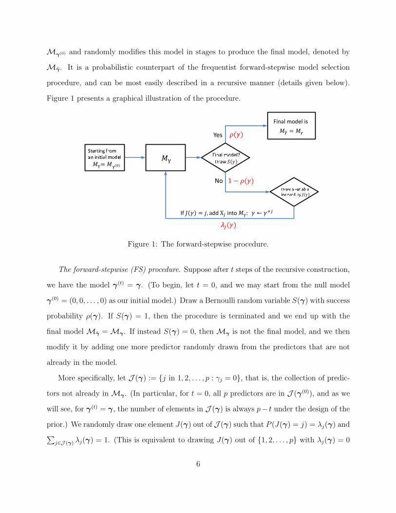
Mγ(0) and randomly modifies this model in stages to produce the final model, denoted by

Mγ. It is a probabilistic counterpart of the frequentist forward-stepwise model selection

procedure, and can be most easily described in a recursive manner (details given below).

Figure 1 presents a graphical illustration of the procedure.

Figure 1: The forward-stepwise procedure.

The forward-stepwise (FS) procedure. Suppose after t steps of the recursive construction,

we have the model γ(t) = γ. (To begin, let t = 0, and we may start from the null model

γ(0) = (0, 0, . . . , 0) as our initial model.) Draw a Bernoulli random variable S(γ) with success

probability ρ(γ). If S(γ) = 1, then the procedure is terminated and we end up with the

final model Mγ = Mγ. If instead S(γ) = 0, then Mγ is not the final model, and we then

modify it by adding one more predictor randomly drawn from the predictors that are not

already in the model.

More specifically, let J (γ) := j in 1, 2, . . . , p : γj = 0, that is, the collection of predic-

tors not already in Mγ. (In particular, for t = 0, all p predictors are in J (γ(0)), and as we

will see, for γ(t) = γ, the number of elements in J (γ) is always p− t under the design of the

prior.) We randomly draw one element J(γ) out of J (γ) such that P (J(γ) = j) = λj(γ) and∑

j∈J (γ) λj(γ) = 1. (This is equivalent to drawing J(γ) out of 1, 2, . . . , p with λj(γ) = 0

6

for all j /∈ J (γ).) If J(γ) = j, then we add Xj into Mγ to get a new model Mγ(t+1) . That is,

we let γ(t+1) = (γ(t+1)1 , γ

(t+1)1 , . . . , γ

(t+1)p ) be such that γ

(t+1)l = γl for all l 6= j and γ

(t+1)j = 1.

From now on we shall use γ+j to denote the indicator vector of this new model, where the

superscript “+j” stands for the additional inclusion of variable Xj into Mγ. This com-

pletes the (t + 1)th step of the recursive construction. The procedure then repeats itself on

γ(t+1) = γ+j, starting from the drawing of a stopping variable, until it eventually stops and

produces the final model Mγ. Note that if the procedure does not stop in the first p steps,

then it will reach the full model, γ(p) = γfull = (1, 1, . . . , 1). Because no further variables

can be added, we must have ρ(γfull) = 1 by design so the procedure always terminates.

Definition 1. A model Mγ, or equivalently a vector γ in 0, 1p, that arises from the

above random recursive procedure is said to have a forward-stepwise (FS) distribution. The

corresponding parameters for such a distribution are the stopping probability ρ(γ) and the

selection probabilities λ(γ) := λj(γ) : j ∈ J (γ), for each Mγ ∈ ΩM.

The stopping probabilities and the selection probabilities in the FS procedure characterize

two key aspects of model selection—the former on the size or complexity of the model

generated and the latter on the relevant predictors to be included, the order of their inclusion,

and the conditional inclusion probability given the variables already included in the model.

Later we will see through examples how we may incorporate prior information regarding

these aspects of the model through proper specification of these parameters.

2.2 Relationship to other model space priors

While the construction of the FS distribution seems quite peculiar, as is stated in the next

theorem, this class of distributions is actually as rich as it can possibly be: all probability

distributions—in particular all prior and posterior distributions—on the model space ΩM

belong to this class. Thus we lose no generality by considering Bayesian variable selection

7

with priors under the FS representation. (A proof is given in the Supplementary Materials.)

Theorem 1 (Generality of the FS distribution). All probability measures on ΩM are FS

distributions. That is, all distributions on ΩM can be represented by a FS procedure with the

corresponding parameters.

Remark: Note that this theorem only establishes the existence of an FS representation for

any given distribution on ΩM. It does not establish the uniqueness. In fact, different FS

procedures may give rise to the same model space distribution. To understand this, note that

the FS procedure generates samples on the “expanded model space” that incorporates the

order of variable inclusions. The induced FS distribution on ΩM is in essence the marginal

distribution on the model space after integrating out the different orderings.

Because the parameters ρ and λ directly correspond to two important aspects of model

selection decisions—model complexity and conditional inclusion probabilities of the predic-

tors, the FS representation can be used to motivate the choice of model space priors. For

example, a useful way to specify the prior stopping probabilities is to let ρ(γ) ≡ ρ|γ| where

|γ| denote the number of 1’s in γ or the number of predictors in Mγ. One could let ρs ≡ ρ,

a constant in [0, 1) for all s = 0, 1, 2, . . . p − 1. For values of ρ not too close to zero, this

imposes further parsimony over the size of the model than what is implicit through the use

of marginal likelihoods (Berger and Pericchi, 2001), as the total prior probability for models

including s predictors is ρ(1 − ρ)s for s < p and (1 − ρ)s for s = p. The prior expected size

of the model is thus (1/ρ − 1)[1 − (1 − ρ)p] which is decreasing in ρ and is close to 1/ρ − 1

for large p. To impose even stronger parsimony over the model size, one can let ρs be an

increasing function in s, such as ρs = 1 − e−as for some positive constant a.

Other choices for ρs can be used to incorporate different prior knowledge (or lack of

knowledge) about the model size. For example, if one believes that the actual model size is

between kmin and kmax where 0 ≤ kmin ≤ kmax ≤ p, but has no a priori reason to prefer any

one particular model size in this range over another, then one may wish to assign uniform

8

prior probability for the model size on the support kmin, kmin + 1, . . . , kmax. This can be

achieved by letting ρs = 0 for s < kmin, and ρs = 1/(kmax − s + 1) for kmin ≤ s ≤ kmax. In

particular, if one wishes to assign uniform prior probability on 0, 1, 2, . . . , p for the model

size, then one can let ρs = 1/(p − s + 1) for all s.

For the prior values of λj(γ), a simple choice is the uniform selection probabilities, that

is, to let λj(γ) ≡ 1/|J (γ)| for all j ∈ J (γ) and all γ ∈ Ωγ. This assumes no prior

knowledge about any particular predictor being more likely to be included than others. More

sophisticated choices of the prior selection probabilities may be used to take into account

the dependence structure among the predictors. For example, one may want to impose

the constraint that the conditional inclusion probability of a predictor that represents an

interaction be zero unless the corresponding main effects have been included in the model.

A more sophisticated example involves the so-called “dilution effect”, which arises from

strong correlation among the predictors as noted in George (1999) and George (2010). We

will devote Section 4 to illustrating how this effect can be accounted in the FS framework.

Note that if one adopts ρ(γ) ≡ ρ|γ| and the uniform values on λ(γ) as described above,

then by symmetry, the prior probability mass on each model of size t is

π(Mγ) = ρt

t−1∏

s=1

(1 − ρs)/

(

p

t

)

for all γ such that |γ| = t.

Any symmetric prior over ΩM—symmetric in the sense that any two models of the same

size receive equal prior probability—can thus be represented with appropriate choices of the

stopping probabilities ρ0, ρ1, . . . , ρp−1.

2.3 Bayesian variable selection with FS priors

Next we investigate how to draw inference using the FS representation for model space priors.

First note that one can of course still apply any of the existing methods for variable selection

9

based on sampling methods to a prior specified under the FS representation. But we will see

that the FS representation leads to an entirely new set of inferential tools that do not rely

on any sampling algorithms. More specifically, we will see that under the FS representation,

the posterior for any prior can be calculated analytically through a sequence of recursion.

The rest of this subsection is devoted to establishing this essential result.

Suppose a model Mγ is generated from an FS procedure. Also, suppose during the

corresponding recursive procedure, after t steps of recursion, we arrive at a model Mγ(t) =

Mγ. If S(γ) = 1, then Mγ = Mγ is the final model, and again we let θγ denote the

corresponding regression coefficients and variance, drawn from a prior p(θγ|Mγ). In this

case the likelihood under the final model is p(Y |θγ,Mγ). If instead S(γ) = 0, then Mγ

is not the final model. In this case, the final model Mγ, and thus the likelihood under it,

depends on further steps of the recursion procedure as characterized by the stopping and

selection variables.

The above description can be represented mathematically also in a recursive manner. For

any model Mγ of size t, we let q(γ|γ) denote the likelihood under the final model Mγ given

that the FS procedure does not terminate in the first t steps and the model reached at the

tth step is Mγ(t) = Mγ. Then we have

q(γ|γ) =

p(Y |θγ,Mγ) if S(γ) = 1 and the model coefficients are θγ

q(γ|γ+J(γ)) if S(γ) = 0 and the next variable to include is J(γ),

or equivalently,

q(γ|γ) = S(γ)p(Y |θγ,Mγ) + (1 − S(γ))q(γ|γ+J(γ)). (2)

10

Note that the likelihood q(γ|γ) is determined by γ along with the following sets of variables

Sγ⊂ = S(γ∗) for all Mγ∗ containing Mγ as a submodel

Jγ⊂ = J(γ∗) for all Mγ∗ containing Mγ as a submodel

θγ⊂ = θγ∗ for all Mγ∗ containing Mγ as a submodel.

That is, it depends on the stopping and selection variables along with the regression coeffi-

cients and variance for all models containing Mγ as a submodel.

Now we define Φ(γ) to be the marginal likelihood under the final model Mγ integrated

over the FS procedure given that the procedure does not stop in the first t steps and Mγ(t) =

Mγ. That is,

Φ(γ) =

∫ ∫

q(γ|γ)p(dθγ|Mγ)π(dMγ|γ(t) = γ)

=∑

γ:Mγ⊂Mγ

∫

q(γ|γ)p(dθγ|Mγ)π(Mγ|γ(t) = γ)

=∑

sγ⊂ , jγ⊂

∫

q(γ|γ)p(dθγ|Mγ)π(sγ⊂, jγ⊂) (3)

where π(·|γ(t) = γ) denotes the model space prior conditional on that the FS procedure

does not terminate in the first t steps and γ(t) = γ, and it is determined by the prior on

(Sγ⊂,Jγ⊂) denoted by π(sγ⊂, jγ⊂). The last summation is taken over all possible values of

Sγ⊂ and Jγ⊂.

Eqs. (2) and (3) together give rise to a recursive representation of Φ(γ)

Φ(γ) = ρ(γ)p(Y |Mγ) + (1 − ρ(γ))∑

j∈J (γ)

λj(γ)Φ(γ+j), (4)

with the convention that if γ = (1, 1, . . . , 1), the full model, then ρ(γ) = 1 and so Φ(γ) =

11

p(Y |Mγ). Note that in order to carry out this recursion, the marginal likelihood term

p(Y |Mγ) under each Mγ needs to be available. (To this end, convenient choices for the

conditional prior of the regression coefficients include the g-prior (Zellner, 1986) and the

hyper-g prior (Liang et al., 2008). We will adopt these choices in the numerical exam-

ples. More generally one may apply methods such as Laplace’s approximation to calculate

P (Y |Mγ) if other priors for the coefficients are adopted.)

But why do we even care about the Φ(γ) terms? They allow us analytically compute

any model space posterior through recursion! The recipe for achieving this is given in the

following theorem. (A proof is given in the Supplementary Materials.)

Theorem 2 (FS representation of a model space posterior). An FS representation for any

model space posterior can be computed analytically based on an FS representation for the

corresponding prior. Specifically, if the prior can be represented by an FS procedure with

parameters ρ and λ, then the posterior can be represented as follows. For each Mγ ∈ ΩM,

1. Posterior stopping probability:

ρpost(γ) = ρ(γ)p(Y |Mγ)/Φ(γ),

2. Posterior selection probabilities:

λpostj (γ) =

(1 − ρ(γ)) λj(γ)Φ(γ+j)

Φ(γ) − ρ(γ)p(Y |Mγ).

Remark: This theorem gives an analytic representation of the corresponding posterior distri-

bution. It allows us to compute the posterior exactly through the recursion formula Eq. (4),

to sample from this posterior directly by simulating the FS procedure with the updated

parameters, and to compute certain summary statistics analytically without using sampling

at all. These will be illustrated in our numerical examples.

12

Eq. (4) and Theorem 2 can be written in terms of Bayes factors (BFs) with respect to

a base model Mγb. Specifically, if we let Φb(γ) = Φ(γ)/P (Y |Mγb

) and BF(Mγ : Mγb) =

P (Y |Mγ)/P (Y |Mγb), then Eq. (4) becomes

Φb(γ) = ρ(γ)BF(Mγ : Mγb) + (1 − ρ(γ))

∑

j∈J (γ)

λjΦb(γ+j).

Accordingly, the posterior parameter updates in Theorem 2 becomes

ρpost(γ) = ρ(γ)BF(Mγ : Mγb)/Φb(γ) and λpost

j (γ) =(1 − ρ(γ))λj(γ)Φb(γ

+j)

Φb(γ) − ρ(γ)BF(Mγ : Mγb).

Thus one can carry out Bayesian variable selection using priors under the FS representation

completely in terms of the BFs. This will become very handy as it is often easier to compute

the BFs with respect to a baseline model than to compute the marginal likelihoods. (See

Section 3.1.) A simple choice of the baseline model is the null model. We will use this choice

in the rest of this work without further declaration.

2.4 Computational strategies in high-dimensional problems

Computing the exact model space posterior requires enumerating all models, as well as com-

puting and summing the marginal likelihood or Bayes factor for each of them. When the

number of potential predictors p is large (> 30), such brute-force integration is infeasible.

Traditionally, sampling methods such as MCMC are then employed to approximate the

integral through simulation. In a different vein, the FS representation through Eq. (4) con-

verts the problem of integration into one of recursion. Consequently, many computational

strategies for approximating recursive computation on trees can be adopted to effectively

approximate the posterior in high-dimensional problems. These strategies form an alterna-

tive to sampling algorithms such as MCMC and SVS for posterior inference, and hold much

13

promise for Bayesian analysis in high-dimensional settings. While sampling algorithms are

effective in exploring local details of the posterior distribution, approximate recursion algo-

rithms provide a means to learning the global shape of the posterior while avoiding difficulties

in mixing and convergence. When combined, the two types of algorithms can form a powerful

set of Bayesian armory for exploring large multi-modal posterior distributions.

One of the simplest approaches for approximating a recursion is to impose an upper limit

k on the depth of the recursion. We shall refer to this method as k-thresholding. In the

current context, this can be achieved by restricting the support of the prior to models of size

no more than k—simply let ρ(γ) = 1 for each model Mγ of size k. When the underlying

model indeed involves no more than k predictors (essentially a sparsity assumption), such an

assumption will actually result in a gain in statistical power in selecting the “true” model. If

otherwise, the “true” model falls out of the support of the posterior, but the method will still

identify relevant sub-models of size no more than k. If desired, one may then keep all the

variables with moderate to high marginal inclusion probabilities as estimated by draws from

the approximate posterior, (which effectively serves as a dimensionality reduction step,) and

carry out another round of selection on that sub-space of models spanned by these “candidate

variables” with a larger model size limit.

A more involved approximation technique, the k-step look-ahead, is a generalization of

k-thresholding. More specifically, one can start by imposing a size limit k on the support of

the FS procedure. After computing the corresponding posterior through a k-level recursion,

one can identify one or a small number of candidate “representative” models that receive high

posterior probability. One can then place a new “local” prior under the FS representation

with size limit k further along the branch of each of those models, and carry out another

iteration of k-level recursion to find its posterior. This procedure continues until the local FS

posteriors suggest termination through the posterior stopping probabilities. The reasoning

behind this algorithm is that large models typically involve good sub-models. Through this

14

procedure, one can effectively zoom into the parts of the model space that are likely to

receive the highest posterior probability.

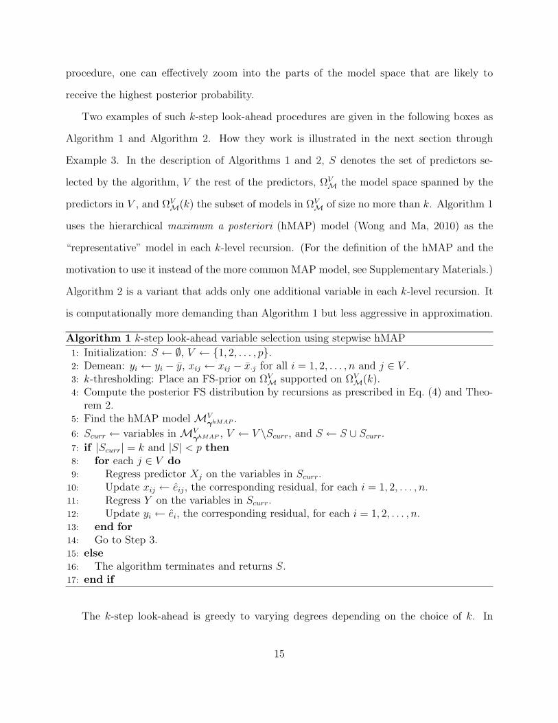
Two examples of such k-step look-ahead procedures are given in the following boxes as

Algorithm 1 and Algorithm 2. How they work is illustrated in the next section through

Example 3. In the description of Algorithms 1 and 2, S denotes the set of predictors se-

lected by the algorithm, V the rest of the predictors, ΩVM the model space spanned by the

predictors in V , and ΩVM(k) the subset of models in ΩV

M of size no more than k. Algorithm 1

uses the hierarchical maximum a posteriori (hMAP) model (Wong and Ma, 2010) as the

“representative” model in each k-level recursion. (For the definition of the hMAP and the

motivation to use it instead of the more common MAP model, see Supplementary Materials.)

Algorithm 2 is a variant that adds only one additional variable in each k-level recursion. It

is computationally more demanding than Algorithm 1 but less aggressive in approximation.

Algorithm 1 k-step look-ahead variable selection using stepwise hMAP

1: Initialization: S ← ∅, V ← 1, 2, . . . , p.2: Demean: yi ← yi − y, xij ← xij − x·j for all i = 1, 2, . . . , n and j ∈ V .3: k-thresholding: Place an FS-prior on ΩV

M supported on ΩVM(k).

4: Compute the posterior FS distribution by recursions as prescribed in Eq. (4) and Theo-rem 2.

5: Find the hMAP model MVγhMAP .

6: Scurr ← variables in MVγhMAP , V ← V \Scurr, and S ← S ∪ Scurr.

7: if |Scurr| = k and |S| < p then

8: for each j ∈ V do

9: Regress predictor Xj on the variables in Scurr.10: Update xij ← eij, the corresponding residual, for each i = 1, 2, . . . , n.11: Regress Y on the variables in Scurr.12: Update yi ← ei, the corresponding residual, for each i = 1, 2, . . . , n.13: end for

14: Go to Step 3.15: else

16: The algorithm terminates and returns S.17: end if

The k-step look-ahead is greedy to varying degrees depending on the choice of k. In

15

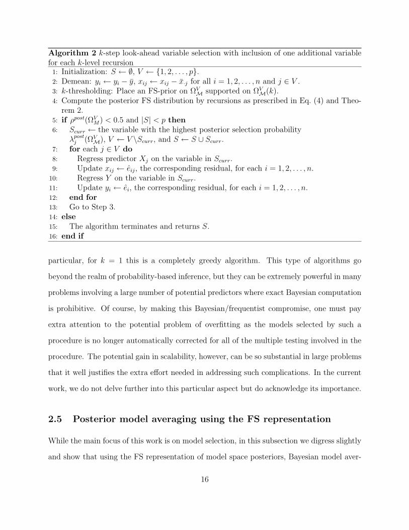
Algorithm 2 k-step look-ahead variable selection with inclusion of one additional variablefor each k-level recursion1: Initialization: S ← ∅, V ← 1, 2, . . . , p.2: Demean: yi ← yi − y, xij ← xij − x·j for all i = 1, 2, . . . , n and j ∈ V .3: k-thresholding: Place an FS-prior on ΩV

M supported on ΩVM(k).

4: Compute the posterior FS distribution by recursions as prescribed in Eq. (4) and Theo-rem 2.

5: if ρpost(ΩVM) < 0.5 and |S| < p then

6: Scurr ← the variable with the highest posterior selection probabilityλpost

j (ΩVM), V ← V \Scurr, and S ← S ∪ Scurr.

7: for each j ∈ V do

8: Regress predictor Xj on the variable in Scurr.9: Update xij ← eij, the corresponding residual, for each i = 1, 2, . . . , n.

10: Regress Y on the variable in Scurr.11: Update yi ← ei, the corresponding residual, for each i = 1, 2, . . . , n.12: end for

13: Go to Step 3.14: else

15: The algorithm terminates and returns S.16: end if

particular, for k = 1 this is a completely greedy algorithm. This type of algorithms go

beyond the realm of probability-based inference, but they can be extremely powerful in many

problems involving a large number of potential predictors where exact Bayesian computation

is prohibitive. Of course, by making this Bayesian/frequentist compromise, one must pay

extra attention to the potential problem of overfitting as the models selected by such a

procedure is no longer automatically corrected for all of the multiple testing involved in the

procedure. The potential gain in scalability, however, can be so substantial in large problems

that it well justifies the extra effort needed in addressing such complications. In the current

work, we do not delve further into this particular aspect but do acknowledge its importance.

2.5 Posterior model averaging using the FS representation

While the main focus of this work is on model selection, in this subsection we digress slightly

and show that using the FS representation of model space posteriors, Bayesian model aver-

16

aging (BMA) (Hoeting et al., 1999), which is essentially integration over the posterior, can

also be carried out through recursion. We let ∆ denote a quantity of interest. BMA is based

on the posterior distribution of ∆:

P (∆|Y ) =∑

γ

P (∆|Y ,Mγ)P (Mγ|Y ),

and in particular its posterior expectation

E(∆|Y ) =∑

γ

E(∆|Y ,Mγ)P (Mγ|Y ).

Under an FS representation of the posterior, these two formulas have a recursive represen-

tation as well. To see this, we first define, for each model Mγ, a quantity Ψ(γ) to be the

posterior expectation of ∆ given that Mγ arises during the random procedure that generates

the final model after |γ| steps. Then

Ψ(γ) = ρpost(γ)E(∆|Y ,Mγ) +(

1 − ρpost(γ))

∑

j∈J (γ)

λpostj (γ)Ψ(γ+j). (5)

Note that E(∆|Y ) = Ψ(γ(0)) and so it can be calculated recursively according to Eq. (5). It

follows that the posterior distribution P (∆|Y ) can also be computed this way by setting ∆

to the appropriate indicator function. Therefore, to carry out BMA, we can first use Theo-

rem 1 to recursively compute the corresponding posterior FS representation, then use Eq. (5)

to again recursively compute the model averaged quantities. Note that the existence of such

a recursive representation of BMA suggests that the computational strategies for approxi-

mating recursions introduced previously can also be adopted for carrying out approximate

BMA in high-dimensional problems.

Example 1 (BMA estimation of marginal inclusion probabilities). In this example we use

17

the above recipe to evaluate the posterior marginal inclusion probability of a variable Xi. In

this case, we let ∆ be the indicator for the event Xi is in the final model. For any model

Mγ, we define Ψ(γ) as in Eq. (5). Note that if Mγ contains Xi, then Eq. (5) reduces to

Ψ(γ) = 1. On the other hand, if Mγ does not contain Xi, then E(∆|Y ,Mγ) = 0, and so

Ψ(γ) =(

1 − ρpost(γ))

∑

j∈J (γ)

λpostj (γ)Ψ(γ+j)

=(

1 − ρpost(γ))

λposti (γ) +

∑

j∈J (γ)\i

λpostj (γ)Ψ(γ+j)

.

By the above recursion, we can calculate Ψ(γ(0)), which is exactly the posterior marginal

inclusion probability for variable Xi.

Remark: While the above example shows that marginal inclusion probabilities can be com-

puted recursively under the proposed framework, it does not suggest that this is the most

efficient way to evaluate those probabilities, especially when there are a large number of

potential variables and the investigator wants to evaluate the inclusion probability for each.

An alternative approach is to sample models from the posterior FS procedure, and estimate

the inclusion probabilities using the sample averages. Although some Monte Carlo error will

be introduced, sampling can be a much more efficient approach when there are many predic-

tors. For this reason, in our later numerical examples, we use sampling from the posterior

to estimate the marginal inclusion probabilities.

3 Numerical examples

In this section we use several numerical examples to illustrate variable selection using priors

under the FS representation. We adopt the g-prior and the hyper-g prior on the regression

coefficients and the noise variance given a model Mγ. Such choices are made due to the

18

availability of closed-form marginal likelihoods, P (Y |Mγ), and BFs. First we provide some

brief background in how the marginal likelihood and BFs are computed for the g-prior and

the hyper-g prior. We refer the interested reader to Liang et al. (2008) for more detail.

3.1 Bayes factors under g-prior and hyper-g prior

Given a particular model Mγ, Zellner’s g-prior in its most popular form is the following

prior on the regression coefficients and the noise variance

p(φ) ∝ 1/φ and βγ|φ,Mγ ∼ N(β0γ, g(XT X)−1/φ)

where β0γ and g are hyperparameters. Following the exposition in Liang et al. (2008), we

assume without loss of generality that the predictor variables X1, X2, . . . , Xp have all

been mean centered at zero. Then we can place a common non-informative flat prior on the

intercept α for all models. So p(α, φ) ∝ 1/φ. Under this prior setup, the marginal likelihood

for model Mγ is

p(Y |Mγ) =Γ((n − 1)/2)√

π(n−1)√

n

(

n∑

i=1

(yi − y)2

)−(n−1)/2

· (1 + g)(n−1−|γ|)/2

(

1 + g(1 − R2γ)

)(n−1)/2

where R2γ is the coefficient of determination for model Mγ. If we choose our baseline model

Mγbto be the null model—that is γb = (0, 0, . . . , 0). Then the Bayes factor for a model Mγ

versus Mγbis

BF(Mγ : Mγb) =

(1 + g)(n−1−|γ|)/2

(

1 + g(1 − R2γ)

)(n−1)/2.

Due to the simplicity of the BF in comparison to the marginal likelihood, we will carry out

the inference through Theorem 2 in terms of the BFs.

To avoid undesirable features of the g-priors such as Barlett’s paradox and the informa-

tion paradox (Berger and Pericchi, 2001), Liang et al. (2008) proposed the use of mixtures

19

of g-priors. In particular, they introduced the hyper-g prior, which adopts the following

hyperprior on g:

g

1 + g∼ Beta(1, a/2 − 1).

This prior also renders a closed form representation for the model-specific marginal likelihood,

and thus for the corresponding BFs. In particular, Liang et al. (2008) showed that the BF

of a model Mγ versus the null model Mγbis given by

BF(Mγ : Mγb) =

a − 2

|γ| + a − 2· 2F1

(

(n − 1)/2, 1; (|γ| + a)/2; R2γ

)

where 2F1(·, ·; ·; ·) is the hypergeometric function. More specifically, in the notations of Liang

et al. (2008),

2F1(a, b; c; z) =Γ(c)

Γ(b)Γ(c − b)

∫ 1

0

tb−1(1 − t)c−b−1

(1 − tz)adt.

Programming libraries are available for evaluating this function (Liang et al., 2008).

3.2 Examples

Example 2 (US Crime data). This is a classical data set introduced in Vandaele (1978)

and adopted in many articles including Raftery et al. (1997) and Clyde et al. (2011) to

compare methods for model selection and averaging. This data set contains 15 variables and

so an exhaustive computation of the marginal likelihood of all 215 models is possible. We

place a prior under the FS representation on this model space with constant prior stopping

probability ρs ≡ 0.5 for all s = 0, 2, . . . , p − 1 and uniform prior selection probabilities,

together with a g-prior with g = n on the coefficients for each model. After computing the

corresponding posterior FS representation, we randomly draw from this posterior—through

simulating the FS procedure—10,000 models, and use the sample average to estimate the

marginal inclusion probability of each predictor.

20

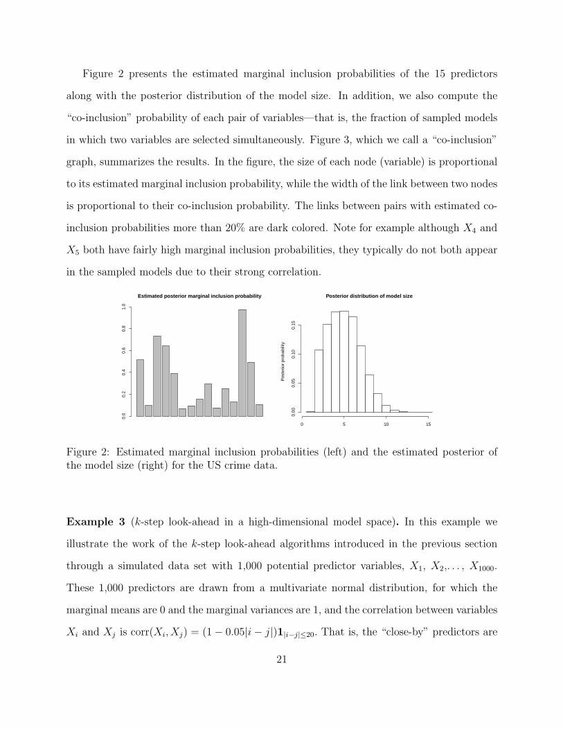
Figure 2 presents the estimated marginal inclusion probabilities of the 15 predictors

along with the posterior distribution of the model size. In addition, we also compute the

“co-inclusion” probability of each pair of variables—that is, the fraction of sampled models

in which two variables are selected simultaneously. Figure 3, which we call a “co-inclusion”

graph, summarizes the results. In the figure, the size of each node (variable) is proportional

to its estimated marginal inclusion probability, while the width of the link between two nodes

is proportional to their co-inclusion probability. The links between pairs with estimated co-

inclusion probabilities more than 20% are dark colored. Note for example although X4 and

X5 both have fairly high marginal inclusion probabilities, they typically do not both appear

in the sampled models due to their strong correlation.

Estimated posterior marginal inclusion probability

0.0

0.2

0.4

0.6

0.8

1.0

Posterior distribution of model size

Model size

Pos

terio

r pr

obab

ility

0 5 10 15

0.00

0.05

0.10

0.15

Figure 2: Estimated marginal inclusion probabilities (left) and the estimated posterior ofthe model size (right) for the US crime data.

Example 3 (k-step look-ahead in a high-dimensional model space). In this example we

illustrate the work of the k-step look-ahead algorithms introduced in the previous section

through a simulated data set with 1,000 potential predictor variables, X1, X2,. . . , X1000.

These 1,000 predictors are drawn from a multivariate normal distribution, for which the

marginal means are 0 and the marginal variances are 1, and the correlation between variables

Xi and Xj is corr(Xi, Xj) = (1 − 0.05|i − j|)1|i−j|≤20. That is, the “close-by” predictors are

21

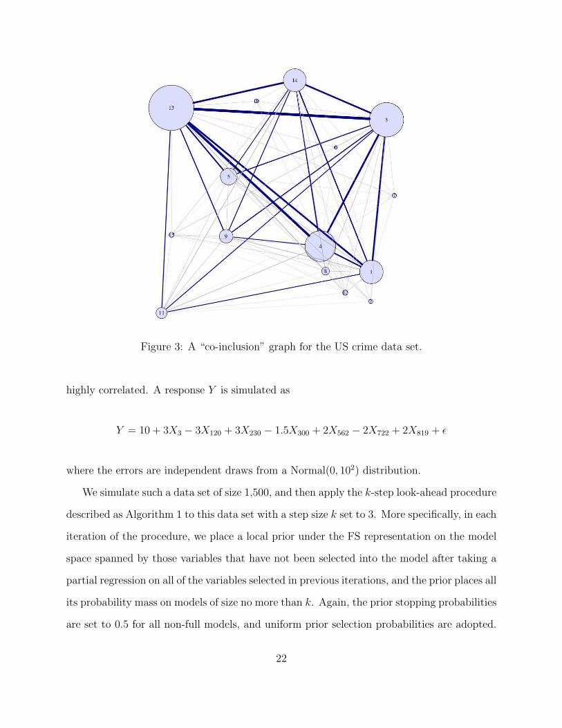
Figure 3: A “co-inclusion” graph for the US crime data set.

highly correlated. A response Y is simulated as

Y = 10 + 3X3 − 3X120 + 3X230 − 1.5X300 + 2X562 − 2X722 + 2X819 + ǫ

where the errors are independent draws from a Normal(0, 102) distribution.

We simulate such a data set of size 1,500, and then apply the k-step look-ahead procedure

described as Algorithm 1 to this data set with a step size k set to 3. More specifically, in each

iteration of the procedure, we place a local prior under the FS representation on the model

space spanned by those variables that have not been selected into the model after taking a

partial regression on all of the variables selected in previous iterations, and the prior places all

its probability mass on models of size no more than k. Again, the prior stopping probabilities

are set to 0.5 for all non-full models, and uniform prior selection probabilities are adopted.

22

A hyper-g prior with a = 3 is placed on the coefficients given each model. After computing

the corresponding posterior FS distribution through recursion, the variables present in the

hMAP model found at each iteration are added into the set of selected variables. Thus

in each iteration at most k variables can be selected. If the hMAP model at an iteration

reaches the maximum size k, then the procedure takes the next iteration and places a new

FS-prior on the model space spanned by the variables not yet selected after taking the partial

regression on the ones already included. This procedure terminates when the hMAP model

at an iteration falls short of the maximum size supported by the prior or the full model has

been reached.

For the current example, the k-step look-ahead terminated after three iterations. In

the first iteration, the hMAP model contains variables X3, X120 and X231. In the second

iteration, variables X560, X722, and X819 are added into the model. Finally, in the third

iteration, a single variable X300 is added and the procedure terminates. (The entire process

took about 5 minutes on a single Intel Core i7 CPU core at 3.8Ghz.) So the “best” model

this procedure selects is Y ∼ X3 + X120 + X231 + X300 + X560 + X722 + X819.

Due to the strong correlation among neighboring markers in this particular simulation

the procedure chose X231 and X560 instead of X230 and X562, but the selected model is indeed

very close to the underlying truth. Note that the algorithm automatically terminated after

three iterations of k-level recursion and the inclusion of the seven relevant variables into the

model. The relevant predictors (or their immediate neighbors) are identified by the algorithm

in an order matching their corresponding effect sizes.

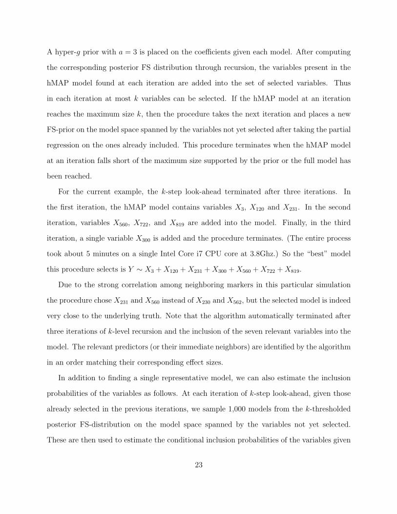
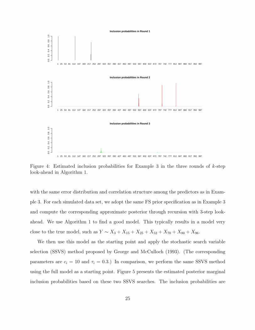
In addition to finding a single representative model, we can also estimate the inclusion

probabilities of the variables as follows. At each iteration of k-step look-ahead, given those

already selected in the previous iterations, we sample 1,000 models from the k-thresholded

posterior FS-distribution on the model space spanned by the variables not yet selected.

These are then used to estimate the conditional inclusion probabilities of the variables given

23

the variables selected in previous steps. We compute the conditional inclusion probability

for each variable not yet in the model in each iteration. The estimated conditional inclusion

probabilities are presented in Figure 4. Due to the correlation among the predictors, the

neighbors of the true predictors of the response also have moderate inclusion probabilities.

Looking at the lower panel in Figure 4, it may seem surprising that in the third iteration

of the k-step algorithm, despite the relatively low inclusion probabilities of all the avail-

able predictors, the algorithm was able to identify X300 in the hMAP model. This shows a

desirable aspect of inference using the FS representation. Although due to the strong cor-

relation among the predictors there are no predictors that stand out as should be included

with high probability, the recursive framework through Eq. (4) allows us to combine the

evidence for the inclusion of an additional predictor from all the neighbors around X300.

As a result, the posterior stopping probability on the model reached after two iterations,

Y ∼ X3 + X120 + X231 + X560 + X722 + X819, is small—about 32%, suggesting the inclusion

of another predictor, and then X300 is chosen as it has the highest conditional inclusion

probability among the variables not in the model. We have also applied Algorithm 2 to the

same simulated data set. The result is very similar and so is not reported here to avoid

redundancy. The performance of the algorithms is consistent across repeated simulations.

Our next example illustrates that one can combine the recursive approach with the stan-

dard sampling methods for inference. In particular, given the model chosen by our method

as a starting point, one can start his/her favorite sampling-based algorithms such as MCMC

or SVS to further explore the posterior around this model. This helps ensure that the chain

starts in a region of “good” models.

Example 4. We simulate data sets of size 1,000 with 100 predictors from the model:

Y = 10 + 3X3 − 3X15 + 3X25 − 1.5X50 + 2X70 − 2X80 + 2X95 + ǫ

24

1 25 53 81 112 147 182 217 252 287 322 357 392 427 462 497 532 567 602 637 672 707 742 777 812 847 882 917 952 987

Inclusion probabilities in Round 1

0.0

0.2

0.4

0.6

0.8

1.0

1 25 53 81 112 147 182 217 252 287 322 357 392 427 462 497 532 567 602 637 672 707 742 777 812 847 882 917 952 987

Inclusion probabilities in Round 2

0.0

0.2

0.4

0.6

0.8

1.0

1 25 53 81 112 147 182 217 252 287 322 357 392 427 462 497 532 567 602 637 672 707 742 777 812 847 882 917 952 987

Inclusion probabilities in Round 3

0.0

0.2

0.4

0.6

0.8

1.0

Figure 4: Estimated inclusion probabilities for Example 3 in the three rounds of k-steplook-ahead in Algorithm 1.

with the same error distribution and correlation structure among the predictors as in Exam-

ple 3. For each simulated data set, we adopt the same FS prior specification as in Example 3

and compute the corresponding approximate posterior through recursion with 3-step look-

ahead. We use Algorithm 1 to find a good model. This typically results in a model very

close to the true model, such as Y ∼ X3 + X15 + X25 + X52 + X70 + X80 + X96.

We then use this model as the starting point and apply the stochastic search variable

selection (SSVS) method proposed by George and McCulloch (1993). (The corresponding

parameters are ci = 10 and τi = 0.3.) In comparison, we perform the same SSVS method

using the full model as a starting point. Figure 5 presents the estimated posterior marginal

inclusion probabilities based on these two SSVS searches. The inclusion probabilities are

25

0 20 40 60 80 100

0.0

0.2

0.4

0.6

0.8

1.0

Predictor

Est

imat

ed m

argi

nal i

nclu

sion

pro

babi

lity

0 20 40 60 80 100

0.0

0.2

0.4

0.6

0.8

1.0

Figure 5: Estimated posterior marginal inclusion probabilities based on two SSVS searches.The solid curve is for the SSVS with the model selected by Algorithm 1 as the starting point.The dashed curve is for the SSVS with the full model as the starting point. The light verticallines indicate the seven predictors in the true model.

estimated based on 2,000 Gibbs iterations with an additional 1,000 burn-in iterations for the

SSVS starting from the full model. While the strong correlation structure makes stochastic

model search very challenging in this example, we can see that the chain that started at the

model selected by our method performs better in terms of sampling around the true model.

We find that if we keep running SSVS chains long enough then the effect of a good starting

point becomes less significant as one would expect. Thus the higher the dimensionality is,

the more important the benefit of a good starting point brings as it will take longer for the

SSVS to get to regions of good models, and take even longer to get reliable estimates of the

inclusion probabilities. We note that Algorithm 1 with 3-step look-ahead takes about two

seconds in this example on a single 3.8Ghz Intel Core-i7 CPU core.

4 Case study: Incorporating model space redundancy

In this subsection we carry out a case study to show that the FS representation of model

space priors provides much flexibility in incorporating prior information. In particular, we

show how one can address an interesting phenomenon called the dilution effect first noted by

26

George (1999). “Dilution” occurs when there is redundancy in the model space. More specif-

ically, consider the scenario where there is strong correlation among some of the predictors,

and any one of these predictors captures virtually all of the association between them and

the response. In this case models that contain different members of this class but are other-

wise identical are essentially the same. As a result, if, say, a symmetric prior specification is

adopted, these models will receive more prior probability than they properly should. At the

same time, other models that do not include members of this class will be down-weighted

in the prior. In real data, this phenomenon occurs to varying degrees depending on the

underlying correlation structure among the predictors.

Next, we present a very simple specification of the FS procedure producing a prior that

can effectively address this phenomenon. We do not claim that this approach is the “best”

way to deal with dilution, but rather use this as an example to illustrate the flexibility

rendered by the FS representation. The specification can be described in two steps.

Step I. Pre-clustering the predictors based on their correlation. First, we carry out a

hierarchical clustering over the predictor variables using the (absolute) correlation as the

similarity metric, which divides the predictors into K clusters—C1, C2, . . . , CK . We recom-

mend using complete linkage as this will ensure that the variables within each cluster are all

very “close” to each other. One needs to choose a correlation threshold s for cutting the cor-

responding dendrogram into clusters—in the case of complete linkage, this is the minimum

correlation for two variables to be in the same cluster. We recommend choosing a large s,

such as 0.9, to place variables into the same basket only if they are highly correlated.

Step II. Specification of the FS prior given the predictor clusters. Based on the predictor

clusters, we assign prior selection probabilities for a model Mγ to the variables not yet in

the model in the following manner. First, we place equal total prior selection probability

over each of the available clusters. Then within each cluster, we assign selection probability

evenly across the variables.

27

For example, consider the situation where there are a total of 10 predictors X1 through

X10, and following Step I, they form four clusters C1 = X1, X2, X3, C2 = X4, X10,

C3 = X5, X7, X9 and C4 = X6, X8. Let Mγ be the model that contains variables X1,

X4, X5, X6, and X8. That is, γ = (1, 0, 0, 1, 1, 1, 0, 1, 0, 0). If the FS procedure reaches Mγ

and the procedure does not stop, that is, S(γ) = 0, then five variables, X2, X3, X7, X9, X10,

from three clusters C ′1 = X2, X3, C ′

2 = X4, and C ′3 = X5 are available for further

inclusion. In this case we choose the selection probabilities λ(γ) to be: λ1(γ) = λ4(γ) =

λ5(γ) = λ6(γ) = λ8(γ) = 0, λ2(γ) = λ3(γ) = 1/3 × 1/2 = 1/6, λ4 = 1/3 and λ5 = 1/3.

Under such a specification, the predictors falling in the same cluster evenly share a fixed

piece of the prior selection probability, which ensures that the prior weight on the other

variables are not “diluted”.

Example 5. We simulate a data set with 60 predictors X1, X2, . . . , X60. They have the

following correlation structure:

corr(Xi, Xj) =

1 − 0.01|i − j| if i = j or maxi, j ≤ 50

0 if i 6= j and maxi, j > 50.

In other words, there is strong correlation among the first 50 predictors X1, X2, . . . , X50

while each of the other 10 variables is independent of all other predictors. We simulate a

response variable Y = 10+4X3 +3X60 + ǫ with ǫ being independent N(0, 102) noise. Due to

the high correlation among X1 through X50, many models that contain different subsets of

them but are otherwise identical are essentially the same. If a symmetric prior specification

is adopted then these models will receive too large a proportion of the prior probability mass.

For example, the first 50 variables possess 5/6 of the prior selection probability to be added

into the null model, while the “effective” number of predictors among them is much smaller.

Consequently, variables X51 to X60 will receive much less prior selection probability than they

28

609 10 7 8 1 2 3 4 5 6

18 19 20 21 22 17 15 16 13 14 11 12 34 35 30 31 32 33 29 27 28 23 24 25 26 47 45 46 50 48 49 38 39 36 37 43 44 42 40 4154 56

5753 58

52 5951 55

10.

80.

60.

40.

20

Cor

rela

tion

Figure 6: Dendrogram for the simulated predictors in Example 5 under complete linkage.The dashed horizontal line indicates the cluster cutoff based on a correlation of 0.9.

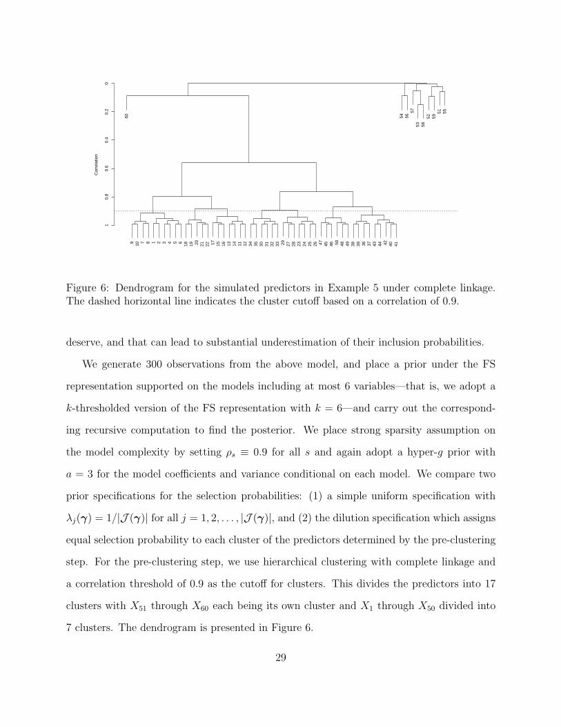
deserve, and that can lead to substantial underestimation of their inclusion probabilities.

We generate 300 observations from the above model, and place a prior under the FS

representation supported on the models including at most 6 variables—that is, we adopt a

k-thresholded version of the FS representation with k = 6—and carry out the correspond-

ing recursive computation to find the posterior. We place strong sparsity assumption on

the model complexity by setting ρs ≡ 0.9 for all s and again adopt a hyper-g prior with

a = 3 for the model coefficients and variance conditional on each model. We compare two

prior specifications for the selection probabilities: (1) a simple uniform specification with

λj(γ) = 1/|J (γ)| for all j = 1, 2, . . . , |J (γ)|, and (2) the dilution specification which assigns

equal selection probability to each cluster of the predictors determined by the pre-clustering

step. For the pre-clustering step, we use hierarchical clustering with complete linkage and

a correlation threshold of 0.9 as the cutoff for clusters. This divides the predictors into 17

clusters with X51 through X60 each being its own cluster and X1 through X50 divided into

7 clusters. The dendrogram is presented in Figure 6.

29

1 7 14 22 30 38 46 54

Inclusion probabilities: dilution

0.0

0.2

0.4

0.6

0.8

1.0

1 7 14 22 30 38 46 54

Inclusion probabilities: symmetric

0.0

0.2

0.4

0.6

0.8

1.0

Posterior for model size: dilution

Den

sity

0 1 2 3 4 5 6

0.0

0.2

0.4

0.6

Posterior for model size: symmetric

Den

sity

0 1 2 3 4 5 60.

00.

20.

40.

6

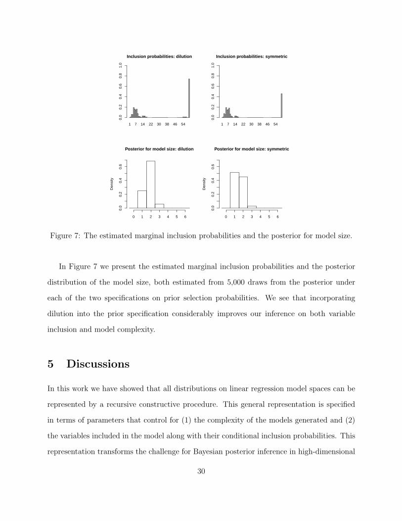
Figure 7: The estimated marginal inclusion probabilities and the posterior for model size.

In Figure 7 we present the estimated marginal inclusion probabilities and the posterior

distribution of the model size, both estimated from 5,000 draws from the posterior under

each of the two specifications on prior selection probabilities. We see that incorporating

dilution into the prior specification considerably improves our inference on both variable

inclusion and model complexity.

5 Discussions

In this work we have showed that all distributions on linear regression model spaces can be

represented by a recursive constructive procedure. This general representation is specified

in terms of parameters that control for (1) the complexity of the models generated and (2)

the variables included in the model along with their conditional inclusion probabilities. This

representation transforms the challenge for Bayesian posterior inference in high-dimensional

30

problems from integration (and sampling) into recursion, and so computational strategies

for approximating recursions can be adopted to exploring the structure of the posterior,

without resorting to sampling algorithms such as MCMC and SVS. This new approach to

posterior inference is in fact complementary to the traditional sampling-based methods. The

approximate recursion methods are effective at learning the global shape of the posterior and

thus can serve as a tool for choosing starting points for sampling methods, which are good

at exploring local features of the posterior.

We note that the construction of the FS procedure can be completely “reversed”—starting

from the full model, which includes all predictors, one can use an analogous recursive pro-

cedure to drop predictors one at a time until stopping. This gives rise to a corresponding

backward-stepwise (BS) representation. Similarly, one can introduce a “two-directional”

representation that also maintains the properties of the FS procedure. To avoid redundancy

in the presentation, we leave the details to the interested reader. The BS procedure is less

useful than the FS as the former imposes a penalty on model simplicity and often favors

more complex models. In the uncommon situation where one has reasons to believe that

the underlying model involves a majority of the potential predictors, however, the BS proce-

dure will be an appropriate choice. In problems with a large number of potential predictors

while the underlying model is expected to involve only a small number of them, the FS

representation seems to be the natural option.

An R package for the introduced method will be available in the near future.

Acknowledgment

The author is thankful to Jim Berger, Merlise Clyde, David Dunson, Fan Li, James Scott,

and Mike West for helpful discussions and comments. The author is especially grateful to

Quanli Wang for help in programming that substantially improved the software efficiency.

31

References

Berger, J. O. and L. R. Pericchi (2001). Objective Bayesian methods for model selection:

Introduction and comparison. Lecture Notes-Monograph Series 38, pp. 135–207.

Carvalho, C. M. and J. G. Scott (2009). Objective bayesian model selection in gaussian

graphical models. Biometrika 96 (3), 497–512.

Chipman, H. (1996). Bayesian variable selection with related predictors. Canadian Journal

of Statistics 24, 17–36.

Clyde, M., H. Desimone, and G. Parmigiani (1996). Prediction via orthogonalized model

mixing. Journal of the American Statistical Association 91 (435), pp. 1197–1208.

Clyde, M. and E. I. George (2000). Flexible empirical Bayes estimation for wavelets. Journal

of the Royal Statistical Society: Series B (Statistical Methodology) 62 (4), 681–698.

Clyde, M. and E. I. George (2004). Model uncertainty. STATIST. SCI 19, 81–94.

Clyde, M. A., J. Ghosh, and M. L. Littman (2011). Bayesian adaptive sampling for variable

selection and model averaging. Journal of Computational and Graphical Statistics 20 (1),

80–101.

Cui, W. and E. I. George (2008). Empirical Bayes vs. fully Bayes variable selection. Journal

of Statistical Planning and Inference 138 (4), 888–900.

Fernndez, C., E. Ley, and M. F. J. Steel (2001). Benchmark priors for Bayesian model

averaging. Journal of Econometrics 100, 381–427.

Foster, D. P. and E. I. George (1994). The risk inflation criterion for multiple regression.

The Annals of Statistics 22 (4), pp. 1947–1975.

32

George, E. I. (1999). Sampling considerations for model averaging and model search. invited

discussion of “Model averaging and model search”, by M. Clyde. In J. M. Bernado, J. O.

Berger, A. P. Dawid, and A. F. M. Smith (Eds.), Bayesian Statistics 6, pp. 175–177.

Oxford, UK: Oxford University Press.

George, E. I. (2010). Dilution priors: Compensating for model space redundancy. In Bor-

rowing Strength: Theory Powering Applications - A Festschrift for Lawrence Brown, pp.

158–165. IMS Collections.

George, E. I., I. George, and D. P. Foster (2000). Calibration and empirical Bayes variable

selection. Biometrika 87, 731–747.

George, E. I. and R. E. McCulloch (1993). Variable Selection Via Gibbs Sampling. Journal

of the American Statistical Association 88 (423), 881–889.

George, E. I. and R. E. McCulloch (1997). Approaches for Bayesian variable selection.

Statistica Sinica 7 (2), 339–373.

Geweke, J. (1996). Variable selection and model comparison in regression. In J. M. Bernado,

J. O. Berger, A. P. Dawid, and A. F. M. Smith (Eds.), Bayesian Statistics 5, pp. 339–348.

Oxford, UK: Oxford University Press.

Hans, C., A. Dobra, and M. West (2007, June). Shotgun Stochastic Search for “Large p”

Regression. Journal of the American Statistical Association 102 (478), 507–516.

Hansen, M. H. and B. Yu (2001). Model selection and the principle of minimum description

length. Journal of the American Statistical Association 96 (454), 746–774.

Hoeting, J. A., D. Madigan, A. E. Raftery, and C. T. Volinsky (1999). Bayesian model

averaging: A tutorial. Statistical Science 14 (4), pp. 382–401.

33

Jones, B., C. Carvalho, A. Dobra, C. Hans, C. Carter, and M. West (2005). Experiments in

stochastic computation for high-dimensional graphical models. Statistical Science 20 (4),

388–400.

Kass, R. E. and L. Wasserman (1995). A reference Bayesian test for nested hypotheses

and its relationship to the Schwarz criterion. Journal of the American Statistical Associ-

ation 90 (431), pp. 928–934.

Leamer, E. E. (1978a). Regression Selection Strategies and Revealed Priors. Journal of the

American Statistical Association 73 (363), 580–587.

Leamer, E. E. (1978b). Specification searches : ad hoc inference with nonexperimental data.

New York: Wiley.

Ley, E. and M. F. Steel (2009). On the effect of prior assumptions in Bayesian model

averaging with applications to growth regression. Journal of Applied Econometrics 24 (4),

651–674.

Li, F. and N. R. Zhang (2010). Bayesian variable selection in structured high-dimensional

covariate spaces with applications in genomics. JASA Theory and Methods 105, 1202–

1214.

Liang, F., R. Paulo, G. Molina, M. A. Clyde, and J. O. Berger (2008). Mixtures of g-Priors

for Bayesian Variable Selection. Journal of the American Statistical Association 103 (481),

410–423.

Mitchell, T. J. and J. J. Beauchamp (1988). Bayesian variable selection in linear regression.

Journal of the American Statistical Association 83 (404), pp. 1023–1032.

Raftery, A. E., D. Madigan, and J. A. Hoeting (1997). Bayesian model averaging for linear

regression models. Journal of the American Statistical Association 92 (437), pp. 179–191.

34

Scott, J. G. and J. O. Berger (2010). Bayes and empirical-Bayes multiplicity adjustment in

the variable-selection problem. ANNALS OF STATISTICS 38, 2587.

Smith, M. and R. Kohn (1996). Nonparametric regression using bayesian variable selection.

Journal of Econometrics 75 (2), 317 – 343.

Stewart, L. and W. W. Davis (1986). Bayesian posterior distributions over sets of possi-

ble models with inferences computed by Monte Carlo integration. Journal of the Royal

Statistical Society. Series D (The Statistician) 35 (2), pp. 175–182.

Vandaele, W. (1978). Participation in illegitimate activities—Ehrlich revisited. In A. Blum-

stein, J. Cohen, and D. Nagin (Eds.), Deterrence and Incapacitation, pp. 270–335. Wash-

ington, DC: National Academy of Sciences Press.

Wong, W. H. and L. Ma (2010). Optional Polya tree and Bayesian inference. Annals of

Statistics 38 (3), 1433–1459.

Zellner, A. (1971). An Introduction to Bayesian Inference in Econometrics. John Wiley and

Sons.

Zellner, A. (1981). Posterior odds ratios for regression hypotheses: General considerations

and some specific results. Journal of Econometrics 16 (1), 151–152.

Zellner, A. (1986). On assessing prior distributions and Bayesian regression analysis with g-

prior distributions. In in Bayesian Inference and Decision Techniques: Essays in Honour

of Bruno de Finetti, pp. 233–243. North-Holland.

Zellner, A. and A. Siow (1980). Posterior odds ratios for selected regression hypotheses.

Bayesian Statistics. Proceedings of the First Valencia International Meeting Held in Va-

lencia (Spain), 585–603.

35