Bayesian Portfolio Analysis

Doron AvramovThe Hebrew University of Jerusalem

and

Guofu ZhouWashington University in St. Louis∗

JEL classification: G11; G12; C11

Keywords: Portfolio choice; Parameter uncertainty; Informative prior beliefs;

Return predictability; Model uncertainty; Learning

First draft: March, 2009Current version: December, 2009

∗We are grateful to Lubos Pastor for useful comments and suggestions as well as Dashan Huang andMinwen Li for outstanding research assistance. to

Corresponding Author: Doron Avramov. Email: davramov@huji.ac.il

Bayesian Portfolio Analysis

This paper reviews the literature on Bayesian portfolio analysis. Information about events,

macro conditions, asset pricing theories, and security-driving forces can serve as useful priors in

selecting optimal portfolios. Moreover, parameter uncertainty and model uncertainty are prac-

tical problems encountered by all investors. The Bayesian framework neatly accounts for these

uncertainties, whereas standard statistical models often ignore them. We review Bayesian portfolio

studies when asset returns are assumed both independently and identically distributed as well as

predictable through time. We cover a range of applications, from investing in single assets and

equity portfolios to mutual and hedge funds. We also outline existing challenges for future work.

Contents

1 Introduction 1

2 Asset Allocation when Returns are IID 2

2.1 The Bayesian Framework . . . . . . . . . . . . . . . . . . . . . . . . . . . . . . . . . 4

2.2 Performance Measures . . . . . . . . . . . . . . . . . . . . . . . . . . . . . . . . . . . 6

2.3 Conjugate Prior . . . . . . . . . . . . . . . . . . . . . . . . . . . . . . . . . . . . . . . 7

2.4 Hyperparameter Prior . . . . . . . . . . . . . . . . . . . . . . . . . . . . . . . . . . . 8

2.5 The Black-Litterman Model . . . . . . . . . . . . . . . . . . . . . . . . . . . . . . . . 9

2.6 Asset Pricing Prior . . . . . . . . . . . . . . . . . . . . . . . . . . . . . . . . . . . . . 11

2.7 Objective Prior . . . . . . . . . . . . . . . . . . . . . . . . . . . . . . . . . . . . . . . 12

3 Predictable Returns 13

3.1 One-Period Models . . . . . . . . . . . . . . . . . . . . . . . . . . . . . . . . . . . . . 13

3.2 Multi-Period Models . . . . . . . . . . . . . . . . . . . . . . . . . . . . . . . . . . . . 15

3.3 Model Uncertainty . . . . . . . . . . . . . . . . . . . . . . . . . . . . . . . . . . . . . 16

3.4 Prior about the Extent of Predictability Explained by Asset Pricing Models . . . . . 18

3.5 Time Varying Beta . . . . . . . . . . . . . . . . . . . . . . . . . . . . . . . . . . . . . 19

3.6 Out-of-sample Performance . . . . . . . . . . . . . . . . . . . . . . . . . . . . . . . . 20

3.7 Investing in Mutual and Hedge Funds . . . . . . . . . . . . . . . . . . . . . . . . . . 21

4 Alternative Data-generating Processes 22

5 Extensions and Future Research 24

6 Conclusion 25

1 Introduction

Portfolio selection is one of the most important problems in practical investment management.

First papers in the field go back at least to the mean variance paradigm of Markowitz (1952)

which analytically formalizes the risk return tradeoff in selecting optimal portfolios. Even when

the mean variance is a static one-period model it has widely been accepted by both academics and

practitioners. The latter developed intertemporal Capital Asset Pricing Model of Merton (1973)

already accounts for the dynamic multi-period nature of investment-consumption decisions. In

an intertemporal economy, the overall demand for risky assets consists of both the mean variance

component as well as a component hedging against unanticipated shocks to time varying investment

opportunities. Empirically, for a wide variety of preferences, hedging demands for risky assets are

typically small, even nonexistent [see also Ait-Sahalia and Brandt (2001) and Brandt (2009)].

We review Bayesian studies of portfolio analysis. The Bayesian approach is potentially attrac-

tive. First, it can employ useful prior information about quantities of interest. Second, it accounts

for estimation risk and model uncertainty. Third, it facilitates the use of fast, intuitive, and easily

implementable numerical algorithms in which to simulate otherwise complex economic quantities.

There are three building blocks underlying Bayesian portfolio analysis. The first is the formation

of prior beliefs, which are typically represented by a probability density function on the stochastic

parameters underlying the stock return evolution. The prior density can reflect information about

events, macroeconomy news, asset pricing theories, as well as any other insights relevant to the

dynamics of asset returns. The second is the formulation of the law of motion governing the evo-

lution of asset returns. Then, one could recover the predictive distribution of future asset returns,

analytically or numerically, incorporating prior information, law of motion, as well as estimation

risk and model uncertainty. The predictive distribution, which integrates out the parameter space,

characterizes the entire uncertainty about future asset returns. The Bayesian optimal portfolio rule

is obtained by maximizing the expected utility with respect to the predictive distribution.

Zellner and Chetty (1965) pioneer the use of predictive distribution in decision-making in gen-

eral. First applications in finance appear during the 1970s. Such applications are entirely based on

uninformative or data based priors. Bawa, Brown, and Klein (1979) provide an excellent survey

on such applications. Jorion (1986) introduces the hyperparameter prior approach in the spirit of

1

the Bayes-Stein shrinkage prior, while Black and Litterman (1992) advocate an informal Bayesian

analysis with economic views and equilibrium relations. Recent studies of Pastor (2000) and Pastor

and Stambaugh (2000) center prior beliefs around values implied by asset pricing theories. Tu and

Zhou (2009) argue that the investment objective itself provides a useful prior for portfolio selection.

Whereas all above-noted studies assume that asset returns are identically and independently

distributed through time, Kandel and Stamabugh (1996), Barberis (2000), and Avramov (2002),

among others, account for the possibility that returns are predictable by macro variables such as

the aggregate dividend yield, the default spread, and the term spread. Incorporating predictability

provides fresh insights into asset pricing in general and Bayesian portfolio selection in particular.

Indeed, we review Bayesian portfolio studies when asset returns are assumed to (i) be indepen-

dently and identically distributed, (ii) be predictable through time by macro conditions, as well as

(iii) exhibit regime shifts and stochastic volatility. We cover a range of applications, from investing

in the market portfolio, equity portfolios, and single stocks to investing in mutual funds and hedge

funds. We also outline existing challenges for future work.

The paper is organized as follows. Section 2 reviews Bayesian portfolio analysis when asset

returns are independent and identically distributed through time. Section 3 surveys studies that

account for potential predictability in asset returns. Section 4 discusses alternative return gener-

ating processes. Section 5 outlines ideas for future research, and Section 6 concludes.

2 Asset Allocation when Returns are IID

Consider N + 1 investable assets, one of which is riskless and the others are risky. Risky assets

may include stocks, bonds, currencies, mutual funds, and hedge funds. Denote by rft and rt the

returns on the riskless and risky assets at time t, respectively. Then, Rt ≡ rt − rft1N is an N

dimensional vector of time t excess returns on risky assets, where 1N is an N -vector of ones. The

joint distribution of Rt is assumed IID through time with mean µ and covariance matrix V.

For analytical insights, it would be beneficial to review the mean-variance framework pioneered

by Markowitz (1952). In particular, consider an optimizing investor who chooses at time T portfolio

2

weights w so as to maximize the quadratic objective function

U(w) = E[Rp]−γ

2Var[Rp] = w′µ− γ

2w′V w, (1)

where E and Var denote the mean and variance of the uncertain portfolio rate of return Rp =

w′RT+1 to be realized in time T + 1, and γ is the relative risk aversion coefficient. It is well-known

that, when both µ and V are known, the optimal portfolio weights are given by

w∗ =1γV −1µ, (2)

and the maximized expected utility is

U(w∗) =1

2γµ′V −1µ =

θ2

2γ, (3)

where θ2 = µ′V −1µ is the squared Sharpe ratio of the ex ante tangency portfolio of the risky assets.

In practice, it is impossible to compute w∗ because µ and V are essentially unknown. Thus,

the mean-variance theory can be applied in two steps. In the first step, the mean and covariance

matrix of asset returns are estimated based on the observed data. Specifically, given a sample of T

observations on asset returns, the standard maximum likelihood estimators are

µ =1T

T∑t=1

Rt, (4)

V =1T

T∑t=1

(Rt − µ)(Rt − µ)′. (5)

Then, in the second step, these sample estimates are treated as if they were the true parameters,

and are simply plugged into (2) to compute the estimated optimal portfolio weights

wML =1γV −1µ. (6)

Of course, the two-step procedure gives rise to a parameter uncertainty problem because it is

the estimated parameters, not the true ones, which are used to compute optimal portfolio weights.

Consequently, the utility associated with the plug-in portfolio weights can be substantially different

from the true utility, U(w∗). In particular, denote by θ the vector of the unknown parameters µ

and V . Mathematically, the two-step procedure maximizes the expected utility conditional on the

estimated parameters, denoted by θ, being equal to the true ones

maxw

[U(w) | θ = θ]. (7)

Thus, estimation risk is altogether ignored.

3

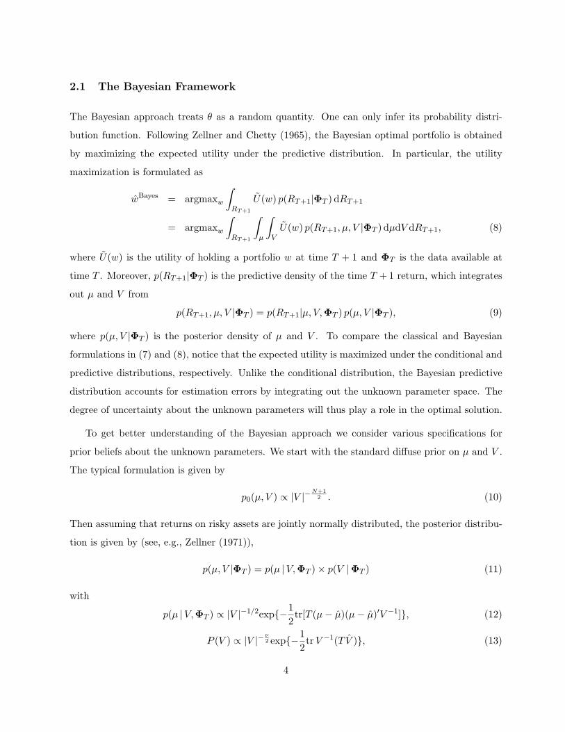
2.1 The Bayesian Framework

The Bayesian approach treats θ as a random quantity. One can only infer its probability distri-

bution function. Following Zellner and Chetty (1965), the Bayesian optimal portfolio is obtained

by maximizing the expected utility under the predictive distribution. In particular, the utility

maximization is formulated as

wBayes = argmaxw

∫RT+1

U(w) p(RT+1|ΦT ) dRT+1

= argmaxw

∫RT+1

∫µ

∫VU(w) p(RT+1, µ, V |ΦT ) dµdV dRT+1, (8)

where U(w) is the utility of holding a portfolio w at time T + 1 and ΦT is the data available at

time T . Moreover, p(RT+1|ΦT ) is the predictive density of the time T + 1 return, which integrates

out µ and V from

p(RT+1, µ, V |ΦT ) = p(RT+1|µ, V,ΦT ) p(µ, V |ΦT ), (9)

where p(µ, V |ΦT ) is the posterior density of µ and V . To compare the classical and Bayesian

formulations in (7) and (8), notice that the expected utility is maximized under the conditional and

predictive distributions, respectively. Unlike the conditional distribution, the Bayesian predictive

distribution accounts for estimation errors by integrating out the unknown parameter space. The

degree of uncertainty about the unknown parameters will thus play a role in the optimal solution.

To get better understanding of the Bayesian approach we consider various specifications for

prior beliefs about the unknown parameters. We start with the standard diffuse prior on µ and V .

The typical formulation is given by

p0(µ, V ) ∝ |V |−N+1

2 . (10)

Then assuming that returns on risky assets are jointly normally distributed, the posterior distribu-

tion is given by (see, e.g., Zellner (1971)),

p(µ, V |ΦT ) = p(µ |V,ΦT )× p(V |ΦT ) (11)

with

p(µ |V,ΦT ) ∝ |V |−1/2exp−12

tr[T (µ− µ)(µ− µ)′V −1], (12)

P (V ) ∝ |V |−ν2 exp−1

2trV −1(T V ), (13)

4

where ‘tr’ denotes the trace of a matrix and ν = T + N . Moreover, the predictive distribution

obeys the expression

p(RT+1|ΦT ) ∝∣∣V + (RT+1 − µ)(RT+1 − µ)′/(T + 1)

∣∣−T/2 , (14)

which amounts to a multivariate t-distribution with T −N degrees of freedom.

The problem of estimation error is already recognized by Markowitz (1952). Nevertheless,

this problem receives serious attention only during the 1970s. Winkler (1973) and Winkle and

Barry (1975) are earlier examples of Bayesian studies on portfolio choice. Brown (1976, 1978) and

Klein and Bawa (1976) lay out independently and clearly the Bayesian predictive density approach,

especially Brown (1976) who explains thoroughly the estimation error problem and the associated

Bayesian approach. Later, Bawa, Brown, and Klein (1979) provide an excellent review of the

literature.

Under the diffuse prior, (10), it is known that the Bayesian optimal portfolio weights are

wBayes =1γ

(T −N − 2T + 1

)V −1µ. (15)

Similar to the classical solution wML, an optimizing Bayesian agent holds the portfolio that is

also proportional to 1γ V−1µ, with the coefficient of proportion being (T − N − 2)/(T + 1). This

coefficient can be substantially smaller than one when N is large relative to T . Intuitively, the

assets are riskier in a Bayesian framework since parameter uncertainty is an additional source of

risk and this risk is accounted for in the portfolio decision. As a result, in the presence of a risk-free

security the overall positions in risky assets are generally smaller in the Bayesian versus classical

frameworks.

However, the Bayesian approach based on diffuse prior does not yield significantly different

portfolio decisions compared with the classical framework. In particular, wML is a biased estimator

of w∗ , whereas the classical unbiased estimator is given by

w =1γ

T −N − 2T

V −1µ, (16)

which is a scalar adjustment of wML, and differs from the Bayesian counterpart only by a scalar

T/(T+1). The difference is independent of N , and is negligible for all practical sample sizes. Hence,

incorporating parameter uncertainty makes little difference if the diffuse prior is used. Indeed, to

5

exhibit the decisive advantage of the Bayesian portfolio analysis, it is essential to elicit informative

priors which account for events, macro conditions, asset pricing theories, as well as any other

insights relevant to the evolution of stock prices.

2.2 Performance Measures

How can one argue that an informative prior is better than the diffuse prior? In general, it is

difficult to make a strong case for a prior specification, because what is good or bad has to be

defined and the definition may not be agreeable among investors. Moreover, ex ante, it is difficult

to know which prior is closer to the true data-generating process.

Following McCulloch and Rossi (1990), Kandel and Stambaugh (1996) and Pastor and Stam-

baugh (2000), among others, focus on utility differences for motivating a performance metric. To

illustrate, let wa and wb be the Bayesian optimal portfolio weights under priors a and b, and let Ua

and Ub be the associated expected utilities evaluated by using the predictive density under prior a.

Then the difference in the expected utilities,

CER = Ua − Ub, (17)

is interpreted as the certainty equivalent return (CER) loss perceived by an investor who is forced

to accept the portfolio selection wb even when wa would be the ultimate choice. The CER is

nonnegative by construction. Indeed, the essential question is how big this value is. Generally

speaking, values over a couple of percentage points per year are deemed economically significant.

However, it should be emphasized that the CER does not say prior a is better or worse than

prior b. It merely evaluates the expected utility differential if prior b is used instead of prior a,

even when prior a is perceived to be the right one. Recall, the true model is unknown, and neither

is known which one of the priors is more informative about the true data-generating process.

Following the statistical decision literature (see, e.g., Lehmann and Casella (1998)), we can

nevertheless use a loss function approach to distinguish the outcomes of using various priors. The

prior that generates the minimum loss is viewed as the best one. In the portfolio choice problem

here, the loss function is well defined. Since any estimated portfolio strategy, w, is a function of

the data, the expected utility loss from using w rather than w∗ is

ρ(w∗, w|µ, V ) ≡ U(w∗)− E[U(w)|µ, V ], (18)

6

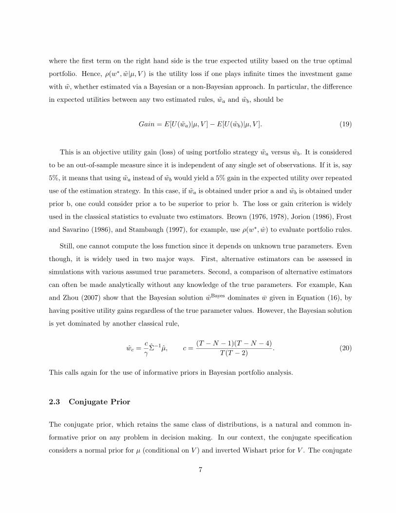
where the first term on the right hand side is the true expected utility based on the true optimal

portfolio. Hence, ρ(w∗, w|µ, V ) is the utility loss if one plays infinite times the investment game

with w, whether estimated via a Bayesian or a non-Bayesian approach. In particular, the difference

in expected utilities between any two estimated rules, wa and wb, should be

Gain = E[U(wa)|µ, V ]− E[U(wb)|µ, V ]. (19)

This is an objective utility gain (loss) of using portfolio strategy wa versus wb. It is considered

to be an out-of-sample measure since it is independent of any single set of observations. If it is, say

5%, it means that using wa instead of wb would yield a 5% gain in the expected utility over repeated

use of the estimation strategy. In this case, if wa is obtained under prior a and wb is obtained under

prior b, one could consider prior a to be superior to prior b. The loss or gain criterion is widely

used in the classical statistics to evaluate two estimators. Brown (1976, 1978), Jorion (1986), Frost

and Savarino (1986), and Stambaugh (1997), for example, use ρ(w∗, w) to evaluate portfolio rules.

Still, one cannot compute the loss function since it depends on unknown true parameters. Even

though, it is widely used in two major ways. First, alternative estimators can be assessed in

simulations with various assumed true parameters. Second, a comparison of alternative estimators

can often be made analytically without any knowledge of the true parameters. For example, Kan

and Zhou (2007) show that the Bayesian solution wBayes dominates w given in Equation (16), by

having positive utility gains regardless of the true parameter values. However, the Bayesian solution

is yet dominated by another classical rule,

wc =c

γΣ−1µ, c =

(T −N − 1)(T −N − 4)T (T − 2)

. (20)

This calls again for the use of informative priors in Bayesian portfolio analysis.

2.3 Conjugate Prior

The conjugate prior, which retains the same class of distributions, is a natural and common in-

formative prior on any problem in decision making. In our context, the conjugate specification

considers a normal prior for µ (conditional on V ) and inverted Wishart prior for V . The conjugate

7

prior is given by

µ |V ∼ N(µ0,1τV ), (21)

V ∼ IW (V0, ν0), (22)

where µ0 is the prior mean, τ is a parameter reflecting the prior precision of µ0, and ν0 is a similar

prior precision parameter on V . Under this prior, the posterior distribution of µ and V obey the

same form as that based on the diffuse prior, except that now the posterior mean of µ is given by

the mixture

µ =τ

T + τµ0 +

T

T + τµ. (23)

That is, the posterior mean is simply a weighted average of the prior and sample means. Similarly,

V0 can be updated by

V =T + 1

T (ν0 +N − 1)

(V0 + T V +

Tτ

T + τ(µ0 − µ)(µ0 − µ)′

), (24)

which is a weighted average of the prior variance, sample variance, and deviations of µ from µ0.

Frost and Savarino (1986) provide an interesting application of the conjugate prior, assuming

all assets exhibit identical means, variances, and patterned covariances, a priori. They find that

such a prior improves ex post performance. This prior is related the well known 1/N rule that

invests equally across the N assets.

2.4 Hyperparameter Prior

Jorion (1986) introduces hyperparameters η and λ that underlie the prior distribution of µ. In

particular, the hyperparameter prior is formulated as

p0(µ | η, λ) ∝ |V |−1exp−12

(µ− η1N )′(λV )−1(µ− η1N ). (25)

Then employing diffuse priors on both η and λ and integrating these parameters out from a suitable

distribution, the predictive distribution of the future portfolio return can be obtained following

Zellner and Chetty (1965). In particular, the Jorion’s optimal portfolio rule is given by

wPJ =1γ

(V PJ)−1µPJ, (26)

8

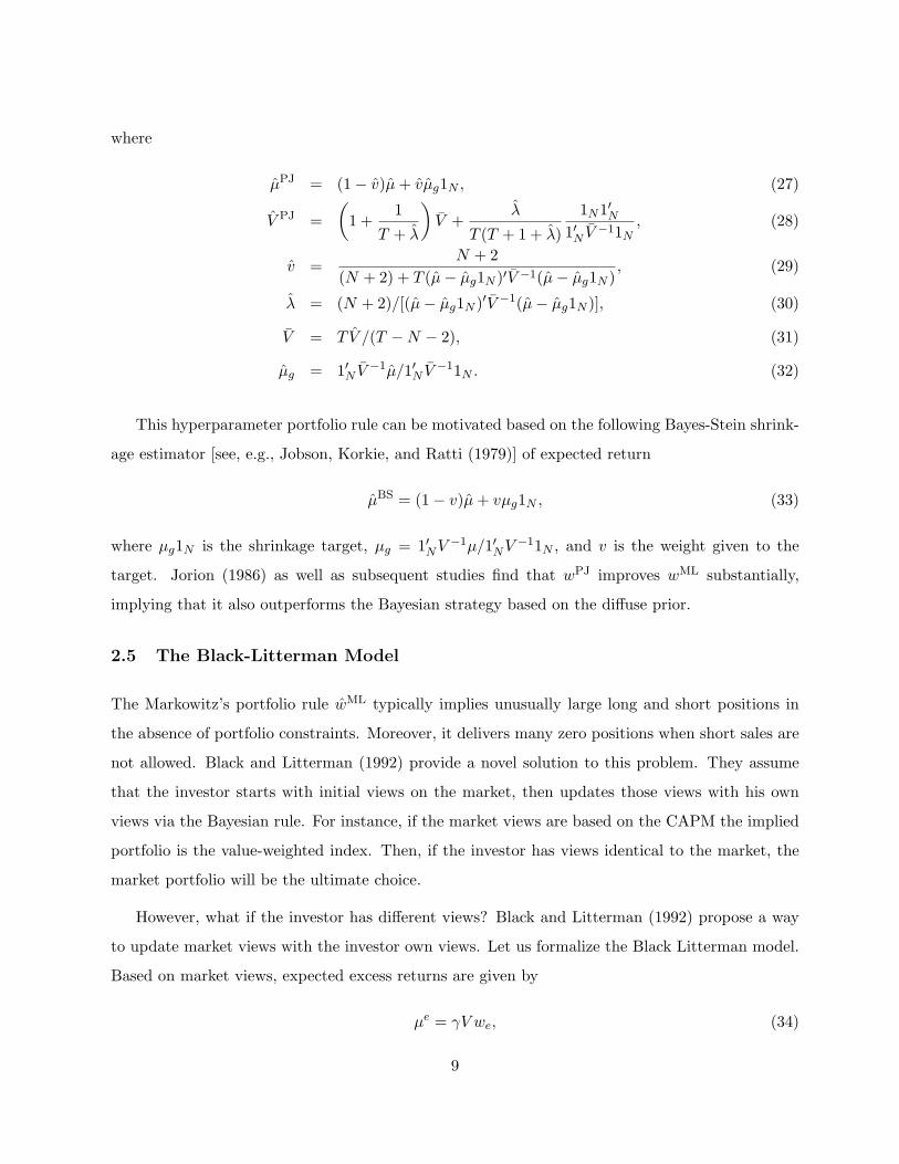
where

µPJ = (1− v)µ+ vµg1N , (27)

V PJ =(

1 +1

T + λ

)V +

λ

T (T + 1 + λ)

1N1′N1′N V −11N

, (28)

v =N + 2

(N + 2) + T (µ− µg1N )′V −1(µ− µg1N ), (29)

λ = (N + 2)/[(µ− µg1N )′V −1(µ− µg1N )], (30)

V = T V /(T −N − 2), (31)

µg = 1′N V−1µ/1′N V

−11N . (32)

This hyperparameter portfolio rule can be motivated based on the following Bayes-Stein shrink-

age estimator [see, e.g., Jobson, Korkie, and Ratti (1979)] of expected return

µBS = (1− v)µ+ vµg1N , (33)

where µg1N is the shrinkage target, µg = 1′NV−1µ/1′NV

−11N , and v is the weight given to the

target. Jorion (1986) as well as subsequent studies find that wPJ improves wML substantially,

implying that it also outperforms the Bayesian strategy based on the diffuse prior.

2.5 The Black-Litterman Model

The Markowitz’s portfolio rule wML typically implies unusually large long and short positions in

the absence of portfolio constraints. Moreover, it delivers many zero positions when short sales are

not allowed. Black and Litterman (1992) provide a novel solution to this problem. They assume

that the investor starts with initial views on the market, then updates those views with his own

views via the Bayesian rule. For instance, if the market views are based on the CAPM the implied

portfolio is the value-weighted index. Then, if the investor has views identical to the market, the

market portfolio will be the ultimate choice.

However, what if the investor has different views? Black and Litterman (1992) propose a way

to update market views with the investor own views. Let us formalize the Black Litterman model.

Based on market views, expected excess returns are given by

µe = γV we, (34)

9

where we denotes the value-weighted weights in the stock index and γ is the market risk-aversion

coefficient. Assume that the true expected excess return µ is normally distributed with mean µe,

µ = µe + εe, εe ∼ N(0, τV ), (35)

where εe, the deviation of µ from µe, is normally distributed with zero mean and covariance matrix

τV with τ being a scalar indicating the degree of belief in how close µ is to the equilibrium value µe.

In the absence of any views on future stock returns, and in the special case of τ = 0, the investor’s

portfolio weights must be equal to we, the weights of the value-weighted index.

Black and Litterman (1992) consider views on the relative performance of stocks that can be

represented mathematically by a single vector equation,

Pµ = µv + εv, εv ∼ N(0,Ω), (36)

where P is a K ×N matrix summarizing K views, µv is a K-vector summarizing the prior means

of the view portfolios, and εv is the residual vector. The views may be formed based on news,

events, or analysis on the economy and investable assets. The covariance matrix of the residuals,

Ω, measures the degree of confidence the investor has in his own views. Applying the Bayesian rule

to the beliefs in market equilibrium relationship and investor own views, as formulated in (35) and

(36), Black and Litterman (1992) obtain the Bayesian updated expected returns and risks as

µBL = [(τV )−1 + P ′Ω−1P ]−1[(τV )−1µe + P ′Ω−1µv], (37)

V BL = V + [(τV )−1 + P ′Ω−1P ]−1. (38)

Replacing V by V and plugging these two updated estimates into (6), one obtains the Black and

Litterman solution to the portfolio choice problem.

Note that the Black-Litterman expected return, µBL, is a weighted average of the equilibrium

expected return and the investor’s views about expected return. Intuitively, the less confident

the investor is in his views, the closer µBL is to the equilibrium value, and so the closer the Black-

Litterman portfolio is to we. This is indeed the case as shown mathematically by He and Litterman

(1999). Hence, the Black Litterman model tilts the investor’s optimal portfolio away from the

market portfolio according to the strength of the investor’s views. Since the market portfolio is a

reasonable starting point which takes no extreme positions, any suitably controlled tilt should also

10

yield a portfolio without any extreme positions. This is one of the major reasons making the Black

Litterman model popular in practice.

Whereas the Black Litterman model is considered to be a Bayesian approach, it is not entirely

Bayesian. For one, the data-generating process is not spelled out explicitly. Moreover, the Bayesian

predictive density is not used anywhere. Zhou (2009) treats the investors’ view as yet another layer

of priors, and combines this and the equilibrium prior with the data-generating process, resulting

a formal Bayesian treatment and an extension of the famous Black and Litterman model.

2.6 Asset Pricing Prior

Pastor (2000) and Pastor and Stambaugh (2000) introduce interesting priors that reflect an in-

vestor’s degree of belief in the ability of an asset pricing model to explain the cross section disper-

sion in expected returns. In particular, let Rt = (yt, xt), where yt contains the excess returns of m

non-benchmark positions and xt contains the excess returns of K (= N −m) benchmark positions.

Consider a factor model multivariate regression

yt = α+Bxt + ut, (39)

where ut is an m × 1 vector of residuals with zero means and a non-singular covariance matrix

Σ = V11 −BV22B′. Notice that α and B are related to µ and V through

α = µ1 −Bµ2, B = V12V−1

22 , (40)

where µi and Vij (i, j = 1, 2) are the corresponding partitions of µ and V ,

µ =(µ1

µ2

), V =

(V11 V12

V21 V22

). (41)

A factor-based asset pricing model, such as the three-factor model of Fama and French (1993),

implies the restrictions α = 0 for all non-benchmark assets.

To allow for mispricing uncertainty, Pastor (2000), and Pastor and Stambaugh (2000) specify

the prior distribution of α as a normal distribution conditional on Σ,

α|Σ ∼ N

[0, σ2

α

(1s2

Σ

Σ)]

, (42)

where s2Σ is a suitable prior estimate for the average diagonal elements of Σ. The above alpha-Sigma

link is also explored by MacKinlay and Pastor (2000) in a classical framework. The magnitude of

11

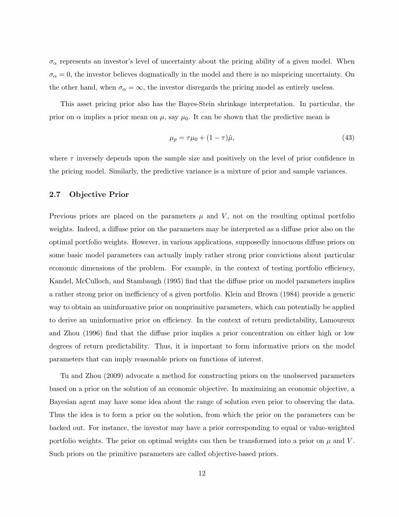
σα represents an investor’s level of uncertainty about the pricing ability of a given model. When

σα = 0, the investor believes dogmatically in the model and there is no mispricing uncertainty. On

the other hand, when σα =∞, the investor disregards the pricing model as entirely useless.

This asset pricing prior also has the Bayes-Stein shrinkage interpretation. In particular, the

prior on α implies a prior mean on µ, say µ0. It can be shown that the predictive mean is

µp = τµ0 + (1− τ)µ, (43)

where τ inversely depends upon the sample size and positively on the level of prior confidence in

the pricing model. Similarly, the predictive variance is a mixture of prior and sample variances.

2.7 Objective Prior

Previous priors are placed on the parameters µ and V , not on the resulting optimal portfolio

weights. Indeed, a diffuse prior on the parameters may be interpreted as a diffuse prior also on the

optimal portfolio weights. However, in various applications, supposedly innocuous diffuse priors on

some basic model parameters can actually imply rather strong prior convictions about particular

economic dimensions of the problem. For example, in the context of testing portfolio efficiency,

Kandel, McCulloch, and Stambaugh (1995) find that the diffuse prior on model parameters implies

a rather strong prior on inefficiency of a given portfolio. Klein and Brown (1984) provide a generic

way to obtain an uninformative prior on nonprimitive parameters, which can potentially be applied

to derive an uninformative prior on efficiency. In the context of return predictability, Lamoureux

and Zhou (1996) find that the diffuse prior implies a prior concentration on either high or low

degrees of return predictability. Thus, it is important to form informative priors on the model

parameters that can imply reasonable priors on functions of interest.

Tu and Zhou (2009) advocate a method for constructing priors on the unobserved parameters

based on a prior on the solution of an economic objective. In maximizing an economic objective, a

Bayesian agent may have some idea about the range of solution even prior to observing the data.

Thus the idea is to form a prior on the solution, from which the prior on the parameters can be

backed out. For instance, the investor may have a prior corresponding to equal or value-weighted

portfolio weights. The prior on optimal weights can then be transformed into a prior on µ and V .

Such priors on the primitive parameters are called objective-based priors.

12

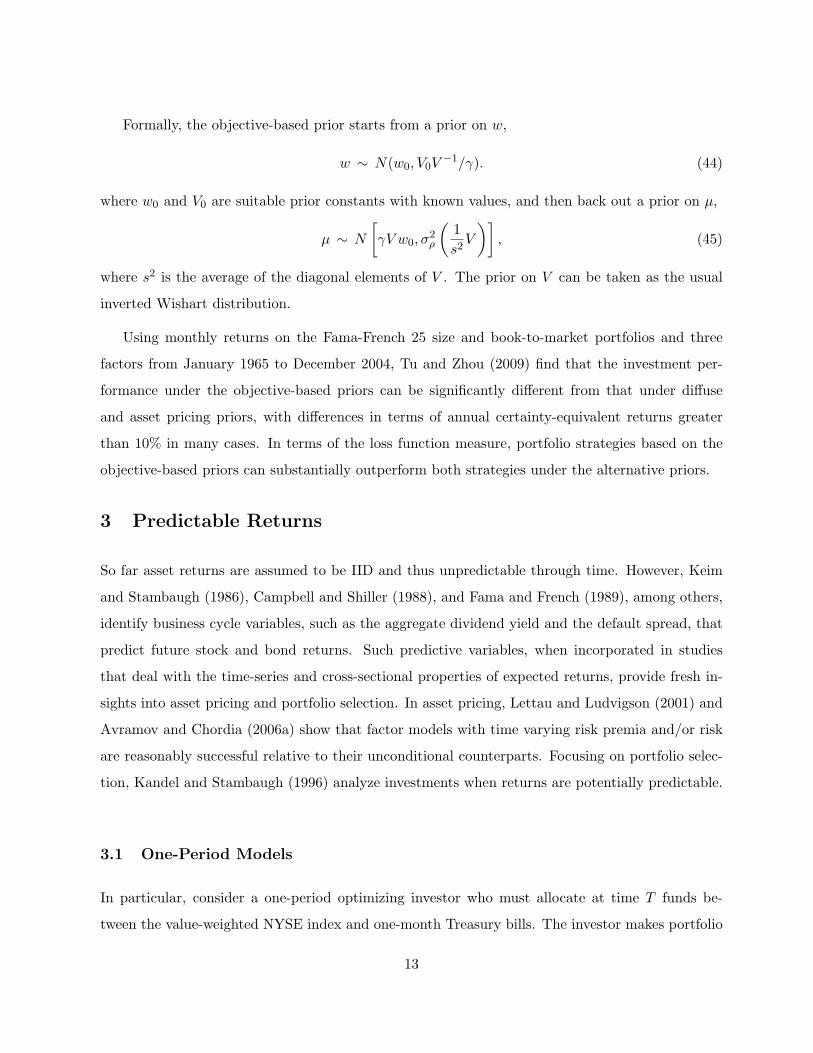
Formally, the objective-based prior starts from a prior on w,

w ∼ N(w0, V0V−1/γ). (44)

where w0 and V0 are suitable prior constants with known values, and then back out a prior on µ,

µ ∼ N

[γV w0, σ

2ρ

(1s2V

)], (45)

where s2 is the average of the diagonal elements of V . The prior on V can be taken as the usual

inverted Wishart distribution.

Using monthly returns on the Fama-French 25 size and book-to-market portfolios and three

factors from January 1965 to December 2004, Tu and Zhou (2009) find that the investment per-

formance under the objective-based priors can be significantly different from that under diffuse

and asset pricing priors, with differences in terms of annual certainty-equivalent returns greater

than 10% in many cases. In terms of the loss function measure, portfolio strategies based on the

objective-based priors can substantially outperform both strategies under the alternative priors.

3 Predictable Returns

So far asset returns are assumed to be IID and thus unpredictable through time. However, Keim

and Stambaugh (1986), Campbell and Shiller (1988), and Fama and French (1989), among others,

identify business cycle variables, such as the aggregate dividend yield and the default spread, that

predict future stock and bond returns. Such predictive variables, when incorporated in studies

that deal with the time-series and cross-sectional properties of expected returns, provide fresh in-

sights into asset pricing and portfolio selection. In asset pricing, Lettau and Ludvigson (2001) and

Avramov and Chordia (2006a) show that factor models with time varying risk premia and/or risk

are reasonably successful relative to their unconditional counterparts. Focusing on portfolio selec-

tion, Kandel and Stambaugh (1996) analyze investments when returns are potentially predictable.

3.1 One-Period Models

In particular, consider a one-period optimizing investor who must allocate at time T funds be-

tween the value-weighted NYSE index and one-month Treasury bills. The investor makes portfolio

13

decisions based on estimating the predictive system

rt = a+ b′zt−1 + ut, (46)

zt = θ + ρzt−1 + vt, (47)

where rt is the continuously compounded NYSE return in month t in excess of the continuously

compounded T-bill rate for that month, zt−1 is a vector of M predictive variables observed at the

end of month t− 1, b is a vector of slope coefficients, and ut is the regression disturbance in month

t. The evolution of the predictive variables is essentially stochastic. Typically a first order vector

autoregression is employed to model that evolution. The residuals in equations (46) and (47) are

assumed to obey the normal distribution. In particular, let ηt = [ut, v′t]′ then ηt ∼ N(0,Σ) where

Σ =[σ2u σuv

σvu Σv

]. (48)

The distribution of rT+1, the time T + 1 NYSE excess return, conditional on data and model

parameters is N(a+ b′zT , σ2u). Assuming the inverted Wishart prior distribution for Σ and multi-

variate normal prior for the intercept and slope coefficients in the predictive system, the Bayesian

predictive distribution P (rT+1|ΦT ) obeys the Student t density. Then, considering a power utility

investor with parameter of relative risk aversion denoted by γ the optimization formulation is

ω∗ = arg maxω

∫rT+1

[(1− ω) exp(rf ) + ω exp(rf + rT+1)]1−γ

1− γP (rT+1|ΦT ) drT+1, (49)

subject to ω being nonnegative. It is infeasible to have analytic solution for the optimal portfi-

olio. However, it can easily be solved numerically. In particular, given G independent draws for

RT+1 from the suitable predictive distribution, the optimal portfolio is found by implementing a

constrained optimization code to maximize the quantity

1G

G∑g=1

(1− ω) exp(rf ) + ω exp(rf ) +R

(g)T+1)

1−γ

1− γ(50)

subject to ω being nonnegative. Kandel and Stambaugh (1996) show that even when the statistical

evidence on predictability, as reflected through the R2 is the regression (46), is weak, the current

values of the predictive variables, zT , can exert a substantial influence on the optimal portfolio.

14

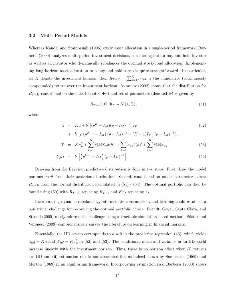
3.2 Multi-Period Models

Whereas Kandel and Stambaugh (1996) study asset allocation in a single-period framework, Bar-

beris (2000) analyzes multi-period investment decisions, considering both a buy-and-hold investor

as well as an investor who dynamically rebalances the optimal stock-bond allocation. Implement-

ing long horizon asset allocation in a buy-and-hold setup is quite straightforward. In particular,

let K denote the investment horizon, then RT+K =∑K

k=1 rT+k is the cumulative (continuously

compounded) return over the investment horizon. Avramov (2002) shows that the distribution for

RT+K conditional on the data (denoted ΦT ) and set of parameters (denoted Θ) is given by

RT+K |,Θ,ΦT ∼ N (λ,Υ) , (51)

where

λ = Ka+ b′[(ρK − IM )(ρ− IM )−1

]zT (52)

+ b′[ρ(ρK−1 − IM

)(ρ− IM )−1 − (K − 1)IM

](ρ− IM )−1θ,

Υ = Kσ2u +

K∑k=1

δ(k)Σvδ(k)′ +K∑k=1

σuvδ(k)′ +K∑k=1

δ(k)σvu, (53)

δ(k) = b′[(ρk−1 − IM

)(ρ− IM )−1

]. (54)

Drawing from the Bayesian predictive distribution is done in two steps. First, draw the model

parameters Θ from their posterior distribution. Second, conditional on model parameters, draw

RT+K from the normal distribution formulated in (51) - (54). The optimal portfolio can then be

found using (50) with RT+K replacing RT+1 and Krf replacing rf .

Incorporating dynamic rebalancing, intermediate consumption, and learning could establish a

non trivial challenge for recovering the optimal portfolio choice. Brandt, Goyal, Santa Clara, and

Stroud (2005) nicely address the challenge using a tractable simulation based method. Pastor and

Veronesi (2009) comprehensively survey the literature on learning in financial markets.

Essentially, the IID set-up corresponds to b = 0 in the predictive regression (46), which yields

λiid = Ka and Υiid = Kσ2u in (52) and (53). The conditional mean and variance in an IID world

increase linearly with the investment horizon. Thus, there is no horizon effect when (i) returns

are IID and (ii) estimation risk is not accounted for, as indeed shown by Samuelson (1969) and

Merton (1969) in an equilibrium framework. Incorporating estimation risk, Barberis (2000) shows

15

that the allocation to equity diminishes with the investment horizon, as stocks appear to be riskier

in longer horizons. Accounting for both return predictability and estimation risk, Barberis (2000)

shows that investors allocate considerably more heavily to equity the longer their horizon.

One essential question is what are the benefits of using the Bayesian approach in studying asset

allocation with predictability?

We describe four major advantages of the Bayesian versus classical approaches. First, unlike

in the single period case wherein estimation risk plays virtually no role, estimation risk does play

an important role in long horizon investment decisions. Barberis shows that a long horizon in-

vestor who ignores it may overallocate to stocks by a sizeable amount. Second, even when the

predictors evolve stochastically, both Kandel and Stambaugh (1996) and Barberis (2000) assume

that the initial value of the predictive variables z0 is non-stochastic. With stochastic initial value

the distribution of future returns conditioned on model parameters does not longer obey a well

known distributional form. Nevertheless, Stambaugh (1999) easily gets around this problem by

implementing the Metropolis Hastings (MH) algorithm, a Markov Chain Monte Carlo procedure

introduced by Metropolis et al (1953) and generalized by Hastings (1970). There are other several

powerful numerical Bayesian algorithms such as the Gibbs Sampler and data augmentation [see

a review by Chib and Greenberg (1996)] which make the Bayesian approach broadly applicable.

The third and fourth advantages pertain to the ability of a Bayesian investor to incorporate model

uncertainty as well as consider prior views about the degree of predictability explained by asset

pricing models. Both of these important features of the Bayesian approach are explained below.

3.3 Model Uncertainty

Indeed, as noted earlier, financial economists have identified economic variables that predict future

asset returns. However, the “correct” predictive regression specification has remained an open is-

sue for several reasons. For one, existing equilibrium pricing theories are not explicit about which

variables should enter the predictive regression. This aspect is undesirable, as it renders the em-

pirical evidence subject to data overfitting concerns. Indeed, Bossaerts and Hillion (1999) confirm

in-sample return predictability, but fail to demonstrate out-of-sample predictability. Moreover, the

multiplicity of potential predictors also makes the empirical evidence difficult to interpret. For ex-

ample, one may find an economic variable statistically significant based on a particular collection of

16

explanatory variables, but often not based on a competing specification. Given that the true set of

predictive variables is virtually unknown, the Bayesian methodology of model averaging, described

below, is attractive, as it explicitly incorporates model uncertainty in asset allocation decisions.

Bayesian model averaging has been implemented to study hearth attacks in medicine, traffic

congestion in transportation economy, hot hands in basketball, and economic growth in macro

economy. In finance, Bayesian model averaging facilitates a flexible modeling of investors uncer-

tainty about potentially relevant predictive variables in forecasting models. In particular, it assigns

posterior probabilities to a wide set of competing return-generating models (Overall, 2M models);

then it uses the probabilities as weights on the individual models to obtain a composite weighted

model. This optimally weighted model is ultimately employed to investigate asset allocation de-

cisions. Bayesian model averaging contrasts markedly with the traditional classical approach of

model selection. In the heart of the model selection approach, one uses a specific criterion (e.g.,

adjusted R2) to select a single model and then operates as if the model is correct. Implementing

model selection criteria, the econometrician views the selected model as the true one with a unit

probability and discards the other competing models as worthless, thereby ignoring model uncer-

tainty. Accounting for model uncertainty, Avramov (2002) shows that Bayesian model averaging

outperforms, ex post out-of-sample, the classical approach of model selection criteria, generating

smaller forecast errors and being more efficient. Ex ante, an investor who ignores model uncertainty

suffers considerable utility loses.

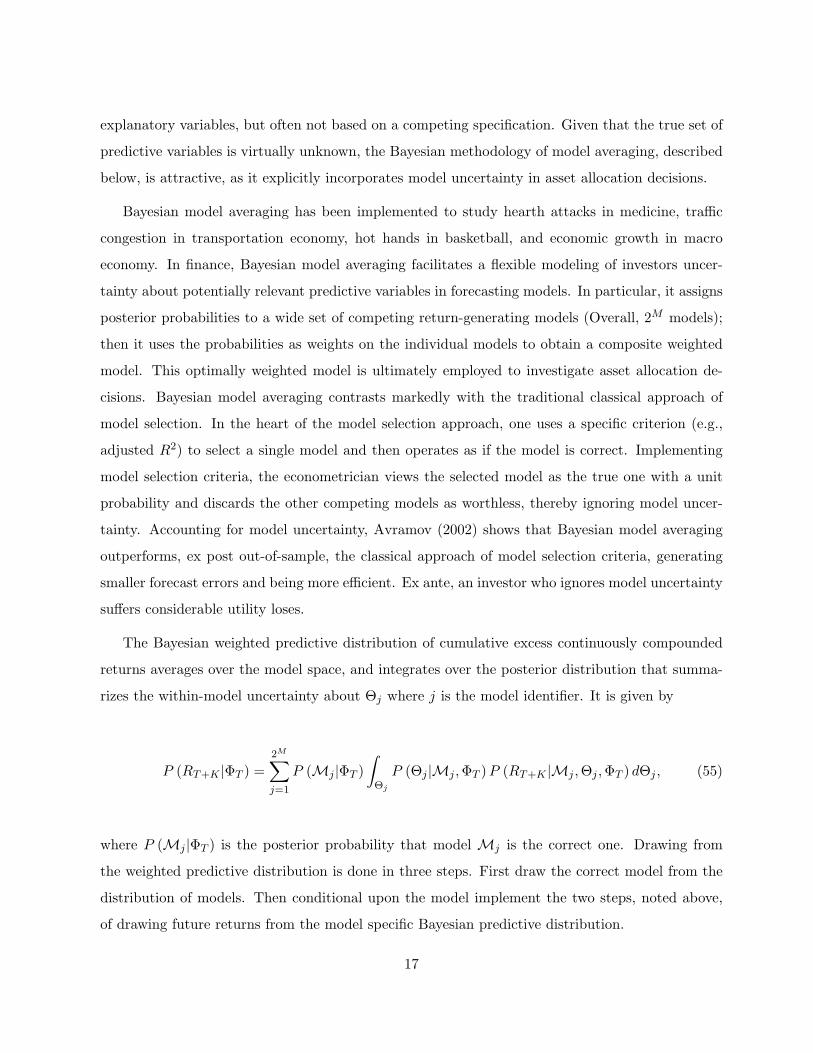
The Bayesian weighted predictive distribution of cumulative excess continuously compounded

returns averages over the model space, and integrates over the posterior distribution that summa-

rizes the within-model uncertainty about Θj where j is the model identifier. It is given by

P (RT+K |ΦT ) =2M∑j=1

P (Mj |ΦT )∫

Θj

P (Θj |Mj ,ΦT )P (RT+K |Mj ,Θj ,ΦT ) dΘj , (55)

where P (Mj |ΦT ) is the posterior probability that model Mj is the correct one. Drawing from

the weighted predictive distribution is done in three steps. First draw the correct model from the

distribution of models. Then conditional upon the model implement the two steps, noted above,

of drawing future returns from the model specific Bayesian predictive distribution.

17

3.4 Prior about the Extent of Predictability Explained by Asset Pricing Models

As noted earlier, the Bayesian approach facilitates incorporating economically motivated priors.

In the context of return predictability, the classical approach has examined whether predictability

is explained by rational pricing or whether it is due to asset pricing misspecification [see, e.g.,

Campbell (1987), Ferson and Korajczyk (1995), and Kirby (1998)]. Studies such as these approach

finance theory by focusing on two polar viewpoints: rejecting or not rejecting a pricing model

based on hypothesis tests. The Bayesian approach incorporates pricing restrictions on predictive

regression parameters as a reference point for a hypothetical investor’s prior belief. The investor

uses the sample evidence about the extent of predictability to update various degrees of belief in

a pricing model and then allocates funds across cash and stocks. Pricing models are expected to

exert stronger influence on asset allocation when the prior confidence in their validity is stronger

and when they explain much of the sample evidence on predictability.

In particular, Avramov (2004) models excess returns on N investable assets as

rt = α(zt−1) + βft + urt, (56)

α(zt−1) = α0 + α1zt−1, (57)

ft = λ(zt−1) + uft, (58)

λ(zt−1) = λ0 + λ1zt−1, (59)

where ft is a set of K monthly excess returns on portfolio based factors, α0 stands for an N -vector

of the fixed component of asset mispricing, α1 is an N ×M matrix of the time varying component,

and β is an N ×K matrix of factor loadings.

Now, a conditional version of an asset pricing model (with fixed beta) implies the relation

E(rt | zt−1) = βλ(zt−1) (60)

for all t, where E stands for the expected value operator. The model (60) imposes restrictions on

parameters and goodness of fit in the multivariate predictive regression

rt = µ0 + µ1zt−1 + vt, (61)

18

where µ0 is an N -vector and µ1 is an N ×M matrix of slope coefficients. In particular, note that

by adding to the right hand side of (61) the quantity β (ft − λ0 − λ1zt−1), subtracting the (same)

quantity βuft, and decomposing the residual in (61) into two orthogonal components vt = βuft+urt,

we reparameterize the return-generating process (61) as

rt = (µ0 − βλ0) + (µ1 − βλ1)zt−1 + βft + urt. (62)

Matching the right-hand side coefficients in (62) with those in (56) yields

µ0 = α0 + βλ0, (63)

µ1 = α1 + βλ1. (64)

The relation (64) indicates that return predictability, if exists, is due to the security-specific

model mispricing component (α1 6= 0) and/or due to the common component in risk premia that

varies (λ1 6= 0). When mispricing is precluded, the regression parameters that conform to asset

pricing models are

µ0 = βλ0 (65)

µ1 = βλ1. (66)

Avramov (2004) shows that asset allocation is extremely sensitive to the imposition of model

restrictions on predictive regressions. Indeed, an investor who believes those restrictions are per-

fectly valid but is forced to allocate funds disregarding model implications faces an enormous utility

loss. Furthermore, asset allocations depart considerably from those dictated by the pricing models

when the prior allows even minor deviations from the underlying models.

3.5 Time Varying Beta

Whereas we have assumed that beta is constant, accounting for time varying beta is straightforward.

Avramov and Chordia (2006b) have modeled the N ×K matrix of factor loadings as

β(zt) = β0 + β1 (IK ⊗ zt) , (67)

where ⊗ denotes the Kronecker product. Avramov and Chordia (2006b) show that the mean and

variance of asset returns in the presence of time varying alpha, beta, and risk premia (assuming

19

informative priors) can be expressed as

µT = α(zT ) + β(zT )(af + AfzT ), (68)

ΣT = P1β(zT )Σff β(zT )′ + P2Ψ, (69)

where the x notation stands for the maximum likelihood estimators, Σff is the covariance matrix

of uft, and Ψ is the covariance matrix of urt, assumed to be diagonal. The predictive variance in

(69) is larger than its maximum likelihood analog as it incorporates the factors P1 and P2, where

P1 is a scalar greater than one and P2 is a diagonal matrix such that each diagonal entry is greater

than one.

3.6 Out-of-sample Performance

Notwithstanding, stock return predictability continues to be a subject of research controversy.

Skepticism exists due to concerns relating to data mining, statistical biases, and weak out-of-sample

performance of predictive regressions as noted by Foster, Smith, and Whaley (1997), Bossaerts and

Hillion (1999), and Stambaugh (1999). Moreover, if firm-level predictability indeed exists, it is not

clear whether it is driven by time varying alpha, beta, or the equity premium.

The ultimate answer is that relative to the IID setup incorporating predictability does improve

performance of investments in equity portfolios, single stocks, mutual funds, and hedge funds.

Focusing on equity portfolios, Avramov (2004) shows that optimal portfolios based on dogmatic

beliefs in conditional pricing models deliver the lowest Sharpe ratios. In addition, completely

disregarding pricing model implications results in the second lowest Sharpe ratios. Remarkably,

much higher Sharpe ratios are obtained when asset allocations are based on the so-called shrinkage

approach, in which inputs for portfolio optimization combine the underlying pricing model and the

sample evidence on predictability. The last two specifications dominate optimal portfolios based

on the IID assumption.

Avramov and Chordia (2006b) show that incorporating business cycle predictors benefits a

real time optimizing investor who must allocate funds across 3,123 NYSE-AMEX stocks and cash.

Investment returns are positive when adjusted by the Fama-French and momentum factors as

well as by the size, book-to-market, and past return characteristics. The investor optimally holds

small-cap, growth, and momentum stocks and loads less (more) heavily on momentum (small-cap)

20

stocks during recessions. Returns on individual stocks are predictable out-of-sample due to alpha

variation. In contrast, beta variation plays no role. Whereas Avramov (2004) and Avramov and

Chordia (2006b) focus on multi security paradigms, Wachter and Warusawitharana (2009) have

documented the superior out of sample performance of the Bayesian approach in market timing.

That is, the equity premium is also predictable by macro conditions.

3.7 Investing in Mutual and Hedge Funds

In an IID setup, Baks, Metrik, and Wachter (2001) (henceforth BMW) have explored the role of

prior information about fund performance in making investment decisions. BMW consider a mean

variance optimizing investor who is skeptical about the ability of a fund manager to pick stocks and

time the market. They find that even with a high degree of skepticism about fund performance the

investor would allocate considerable amounts to actively managed funds.

BMW define fund performance as the intercept in the regression of the fund’s excess returns

on excess return of one or more benchmark assets. Pastor and Stambaugh (2002a,b), however,

recognize the possibility that the intercept in such regressions could be a mix of fund performance

as well as model mispricing. In particular, consider the case wherein benchmark assets used to define

fund performance are unable to explain the cross section dispersion of passive assets, that is, the

sample alpha in the regression of non benchmark passive assets on benchmarks assets is nonzero.

Then model mispricing emerges in the performance regression. Thus, Pastor and Stambaugh

formulate prior beliefs on both performance and mispricing.

Geczy, Stambaugh, and Levin (2005) apply the Pastor Stambaugh methodology to study the

cost of investing in socially responsible mutual funds. Comparing portfolios of these funds to those

constructed from the broader fund universe reveals the cost of imposing the socially responsible

investment (SRI) constraint on investors seeking the highest Sharpe ratio. This SRI cost depends

crucially on the investor’s views about the validity of asset pricing models and managerial skills

in stock picking and market timing. Busse and Irvine (2006) also apply the Pastor Stambaugh

methodology to compare the performance of Bayesian estimates of mutual fund performance with

standard classical based measures using daily data. They find that Bayesian alphas based on the

CAPM are particularly useful for predicting future standard CAPM alphas.

BMW and Pastor and Stambaugh assume that the prior on alpha is independent across funds.

21

However, as shown by Jones and Shanken (2005), under the independence assumption, the maxi-

mum posterior mean alpha increases without bound as the number of funds increases and ”extremely

large” estimates could randomly be generated, even when fund managers have no skill. Instead,

Jones and Shanken (2005) propose incorporating prior dependence across funds. Then, investors

aggregate information across funds to form a general belief about the potential for abnormal perfor-

mance. Each fund’s alpha estimate is shrunk towards the aggregate estimate, mitigating extreme

views.

Avramov and Wermers (2006) and Avramov, Kosowski, Naik, and Teo (2009) extend the

Avramov (2004) methodology to study investments in mutual funds and hedge funds, respectively,

when fund returns are potentially predictable. Avramov and Wermers (2006) show that long-only

strategies that incorporate predictability in managerial skills outperform their Fama-French and

momentum benchmarks by 2 to 4% per year by timing industries over the business cycle, and

by an additional 3 to 6% per year by choosing funds that outperform their industry benchmarks.

Similarly, Avramov, Kosowski, Naik, and Teo (2009) show that incorporating predictability sub-

stantially improves out-of-sample performance for the entire universe of hedge funds as well as for

various investment styles. The major source of investment profitability is again predictability in

managerial skills. In particular, long-only strategies that incorporate such predictability outper-

form their Fung and Hsieh (2004) benchmarks by over 14 percent per year. The economic value of

predictability emerges for different rebalancing horizons and alternative benchmark models. It is

also robust to adjustments for backfill bias, incubation bias, illiquidity, and style composition.

4 Alternative Data-generating Processes

Thus far data-generating processes for asset returns are either IID normal or predictable with

IID disturbances. Such specifications facilitate a tractable implementation of Bayesian portfolio

analysis. To provide a richer model of the interaction between the stock market and economic

fundamentals, Pastor and Stambaugh (2009a) advocate a predictive system allowing aggregate

predictors to be imperfectly correlated with the conditional expected return. Subsequently, Pastor

and Stambaugh (2009b) find that stocks are substantially more volatile over long horizons from an

investor’s perspective, which seems to have profound implications for long-term investments.

22

Incorporating regimes shifts in asset returns is also potentially attractive, as stock prices tend

to persistently rise or fall during certain periods. Tu (2009) extends the asset pricing framework

(39) to capture economic regimes. In particular, he models benchmark and non benchmark assets

as

yt = αst +Bstxt + utst , (70)

where utst is an m × 1 vector with zero means and a non-singular covariance matrix, Σst , and st

is an indicator of the states. Under the usual normal assumption of model residuals, the regime

shift formulation is identical to the specification (39) in each regime. Tu shows that uncertainty

about regime is more important than model mispricing. Hence, the correct identification of the

data-generating process can have significant impact on portfolio choice.

To incorporate latent factors and stochastic volatility in the asset pricing formulation (39), Han

(2006) allows xt in

yt = α+Bxt + ut (71)

to follow the latent process

xt = c+ CXt−1 + vt. (72)

In addition, the vector of residuals ut could display stochastic volatilities. In such a dynamic factor

multivariate stochastic volatility (DFMSV) model, Han finds that the DFMSV dynamic strategies

significantly outperform various benchmark strategies out of sample, and the outperformance is

robust to different performance measures, investor’s objective functions, time periods, and assets.

In addition, Nardari and Scruggs (2007) extend Geweke and Zhou (1996) to provide an alternative

stochastic volatility model with latent asset pricing factors. In their model, mispricing of the

Arbitrage Pricing Theory (APT) pioneered by Ross (1976) can be accommodated.

Since the true data-generating process is unknown, there is an uncertainty about whether a

given process adequately fits the data. For example, previous studies typically assume that stock

returns are conditionally normal. However, the normality assumption is strongly rejected by the

data. Tu and Zhou (2004) find that the t distribution can better fit the data. Kacperczyk (2008)

provides a general framework for treating data-generating process uncertainty.

23

5 Extensions and Future Research

Even when Bayesian analysis of portfolio selection has impressively evolved over the last three

decades, there is still a host of applications of Bayesian methodologies to be carried out. For one,

the Bayesian methodology can be applied to account for estimation risk and model uncertainty

in managing long-short portfolios, international asset allocation, hedge fund speculation, defined

pensions, as well as portfolio selection with various risk controls. In addition, there are still virtually

untouched asset pricing theories to be accounted for in forming informative prior beliefs.

The mean variance utility has long been the baseline for asset allocation in practice. See,

for instance, Grinold and Kahn (1999), Litterman (2003), and Meucci (2005) who discuss various

applications of the mean-variance framework. Indeed, controlling for factor exposures and imposing

trading constraints, among other real time trading impediments, can easily be accommodated

within the mean variance framework with either analytical insights or fast numerical solutions.

In addition, the intertemproal hedging demand is typically small relative to the mean variance

component. Theoretically, however, it would be of interest to consider alternative set of preferences.

Employing alternative utility specifications must be done with extra caution. In particular,

as emphasized by Geweke (2001), the predictive density under iso-elastic preferences is typically

Student t. The unrestricted utility maximization under the t predictive density can have a diver-

gence problem. Nevertheless, the divergence problem could be accounted for by imposing suitable

portfolio constraints. Moreover, for a utility function with up to a given number of moments, the

divergence problem disappears with a suitable adjustment of the degrees of freedom of the t distri-

bution. Harvey, Liechty, Liechty, and Muller (2004) is an excellent example of portfolio selection

with higher moments that has an interpretation well grounded in economic theory. Ang, Bekaert,

and Liu (2005) and Hong, Tu, and Zhou (2007) advocate a Bayesian portfolio analysis that allows

the data-generating process be asymmetric.

A different class of recursive utility functions is found useful in accounting for asset pricing

patterns unexplained by the Capital Asset Pricing Model (CAPM) of Sharpe (1964) and Lintner

(1965) and the consumption based CAPM (CCAPM) of Rubinstein (1976), Lucas (1978), Breeden

(1979), and Grossman and Shiller (1981). In particular, Bansal and Yaron (2004) utilize the

Esptein and Zin (1989) preferences to explain asset pricing puzzles in the aggregate level. Avramov,

24

Cederburg, and Hore (2009) consider the Duffie and Epstein (1992) preferences to explain the

counter intuitive cross sectional negative relations between average stock returns and the three

apparently risk measures (i) credit risk, (ii) dispersion, and (iii) idiosyncratic volatility. Recursive

preferences are also employed by Zhou and Zhu (2009) who are able to justify the large negative

market variance risk premium. Indeed, to our knowledge, there are no Bayesian studies utilizing

the recursive utility framework, nor are there any Bayesian priors that exploit information on such

potentially promising asset pricing models. Future work should form prior beliefs based on long

run risk formulations.

Finally, portfolio analysis based on specifications that departs from IID stock returns (see mul-

tivariate process formulated in Sections 3 and 4) is challenging to solve in multi-period investment

horizons. Much future research in this area is called for.

6 Conclusion

In making portfolio decisions, investors often confront with parameter estimation errors and possible

model uncertainty. In addition, investors may have various prior information on the investment

problem that can arise from news, events, macroeconomic analysis, and asset pricing theories. The

Bayesian approach is well suited for neatly accounting for these features, whereas the classical

statistical analysis disregards any potentially relevant prior information. Hence, Bayesian portfolio

analysis is likely to play an increasing role in making investment decisions in practical investment

management.

While enormous progress has been made in developing various priors and methodologies for

applying the Bayesian approach in standard asset allocation problems, there are still investment

problems that are open for future Bayesian studies. Moreover, much more should be done to allow

Bayesian portfolio analysis to go beyond popular mean-variance utilities as well as consider more

general and realistic data-generating processes.

25

References

Ait-Sahalia, Y., and M., Brandt, 2001, Variable selection for portfolio choice, Journal of Finance

56, 1297-1351.

Ang, Andrew, Geert Bekaert, and Jun Liu, 2005, Why stocks may disappoint, Journal of Financial

Economics 76, 471-508.

Avramov, Doron, 2002, Stock return predictability and model uncertainty, Journal of Financial

Economics 64, 423C458.

Avramov, Doron, 2004, Stock return predictability and asset pricing models, Review of Financial

Studies 17, 699-738.

Avramov, Doron, and Tarun Chordia, 2006a, Asset pricing models and financial market anomalies,

Review of Financial Studies 19,1001-1040.

Avramov, Doron, and Tarun Chordia, 2006b, Predicting stock returns, Journal of Financial Eco-

nomics 82,387-415.

Avramov, Doron, and Russ Wermers, 2006, Investing in mutual funds when returns are pre-

dictable, Journal of Financial Economics 81, 339-377.

Avramov, Doron, Cederburg, Scott, and Satadru Hore, 2009, Cross-sectional asset pricing puzzles:

an equilibrium perspective, Working paper, University of Maryland.

Avramov, Doron, Robert Kosowski, Narayan Naik, and Melvyn Teo, 2009, Hedge funds, manage-

rial skill, and macroeconomic variables, Working Paper, University of Maryland.

Baks, Klaas, Andrew Metrick, and Jessica Wachter, 2001, Should investors avoid all actively

managed mutual funds? A study in Bayesian performance evaluation Journal of Finance 56,

45-85.

Bansal, Ravi, and Amir Yaron, 2004, Risks for the long run: a potential resolution of asset pricing

puzzles, Journal of Finance 59, 1481-1509.

Barberis, Nicholas, 2000, Investing for the long run when returns are predictable, Journal of

Finance 55, 225-264.

26

Bawa, Vijay S., Stephen J. Brown, and Roger W. Klein, 1979, Estimation Risk and Optimal

Portfolio Choice, North-Holland, Amsterdam.

Black, Fischer, and Robert Litterman, 1992, Global portfolio optimization, Financial Analysts

Journal 48, 28-43.

Bossaerts, Peter, and Pierre Hillion, 1999, Implementing statistical criteria to select return fore-

casting models: what do we learn? Review of Financial Studies 12, 405-428.

Brandt, Michael, 2009, Portfolio choice problems, In Handbook of Financial Econometrics Vol

1(1), Y. Ait-Sahalia and L P. Hansen, eds.

Brandt, Michael, Amit Goyal, Pedro Santa-Clara, and Jonathan R. Stroud, 2005, A simulation ap-

proach to dynamic portfolio choice with an application to learning about return predictability,

Review of Financial Studies 18, 831-871.

Breeden, Douglas T., 1979, An intertemporal asset pricing model with stochastic consumption

and investment opportunities, Journal of Financial Economics 7, 265-296.

Brown, Stephen J., 1976, Optimal portfolio choice under uncertainty, Ph.D. dissertation, Univer-

sity of Chicago.

Brown, Stephen J., 1978, The portfolio choice problem: comparison of certainty equivalence and

optimal Bayes portfolios, Communications in Statistics — Simulation and Computation 7,

321-334.

Busse, Jeffrey, and Paul J. Irvine, 2006, Bayesian alphas and mutual fund persistence, Journal of

Finance 61, 2251C2288.

Campbell, John Y., 1987, Stock returns and the term structure, Journal of Financial Economics

18, 373-399.

Campbell, John Y., and Robert J. Shiller, 1988, The dividend ratio model and small sample bias:

a Monte Carlo study, NBER technical working paper.

Chib, Siddhartha, and Edward Greenberg, 1996, Markov Chain Monte Carlo simulation methods

in econometrics, Econometric Theory 12, 409-431.

27

Duffie, Darrell, and Epstein, Larry G, 1992, Asset pricing with Stochastic differential utility,

Review of Financial Studies 5, 411 C 436.

Epstein, Larry G, and Stanley E. Zin, 1989, Substitution, risk aversion, and the temporal behavior

of consumption growth and asset returns I: A theoretical framework, Econoinetrica 57, 937-

969.

Fama, Eugene F., and Kenneth R. French, 1989, Business conditions and expected returns on

stocks and bonds, Journal of Financial Economics 25, 23-49.

Fama, Eugene F., and Kenneth R. French, 1993, Common risk factors in the returns on stocks

and bonds, Journal of Financial Economics 33, 3-56.

Ferson, Wayne E., and Robert A. Korajczyk, 1995, Do arbitrage pricing models explain the

predictability of stock returns? Journal of Business 68, 309-349.

Foster, F. Douglas, Tom Smith, and Robert E. Whaley, 1997, Assessing goodness-of-fit of asset

pricing models: the distribution of the maximal R2, Journal of Finance 52, 591-607.

Frost, Peter A., and James E. Savarino, 1986, An empirical Bayes approach to efficient portfolio

selection, Journal of Financial and Quantitative Analysis 21, 293-305.

Fung, William, and David A. Hsieh, 2004, Hedge fund benchmarks: a risk-based approach, Fi-

nancial Analysts Journal 60, 65-80.

Geczy, Christopher Charles, Stambaugh, Robert F. and Levin, David, 2005, Investing in socially

responsible mutual funds, SSRN working paper.

Geweke, John, 2001, A Note on some limitations of CRRA utility, Economics Letters 71(3), 341-

345.

Geweke, John, and Guofu Zhou, 1996, Measuring the pricing error of the arbitrage pricing theory,

Review of Financial Studies 9, 557-587.

Grinold, Richard C., and Ronald N. Kahn, 1999, Active portfolio management, McGraw-Hill.

Grossman, Sanford J., and Shiller, Robert J., 1981, The determinants of the variability of stock

market prices, American Economic Review 71, 222-227.

28

Han, Yufeng, 2006, Asset allocation with a high dimensional latent factor stochastic volatility

model, Review of Financial Studies 19, 237–271.

Harvey, Campbell R., John C. Liechty, Merrill W. Liechty, and Peter Muller, 2004, Portfolio

selection with higher moments, Working Paper, Duke University.

Hastings, W.K., 1970, Monte Carlo sampling methods using markov chains and their applications,

Biometrika 57, 97-109.

He, Guanliang, and Robert Litterman, 1999, The intuition behind Black-Litterman model port-

folios, Goldman Sachs Quantitative Resources Group working paper.

Hong, Yongmiao, Jun Tu, and Guofu Zhou, 2007, Asymmetries in stock returns: statistical tests

and economic evaluation, Review of Financial Studies 20, 1547-1581.

Jobson, J.D., Bob Korkie, and V. Ratti, 1979, Improved estimation for Markowitz portfolios using

James-Stein type estimators, Proceedings of the American Statistical Association, Business

and Economics Statistics Section 41, 279-284.

Jones, Chris, and Jay Shanken, 2005, Mutual fund performance and learning across funds, Journal

of Financial Economics 78, 507-552

Jorion, Philippe, 1986, Bayes-Stein estimation for portfolio analysis, Journal of Financial and

Quantitative Analysis 21, 279-292.

Kacperczyk, Marcin, 2008, Asset allocation under distribution uncertainty, Working paper, Uni-

versity of British Columbia.

Kan, Raymond, and Guofu Zhou, 2007, Optimal Portfolio Choice with Parameter Uncertainty,

Working paper, Journal of Financial and Quantitative Analysis 42, 621C656.

Kandel, Shmuel, Robert McCulloch, and Robert F. Stambaugh, 1995, Bayesian inference and

portfolio efficiency, Review of Financial Studies 9(1), 1-53.

Kandel, Shmuel, and Robert F. Stambaugh, 1996, On the predictability of stock returns: an

asset-allocation perspective, Journal of Finance 51, 385-424.

29

Keim, Donald B., and Robert F. Stambaugh, 1986, Predicting returns in bond and stock markets,

Journal of Financial Economics 12, 357-390.

Kirby, Chris, 1998, The restrictions on predictability implied by rational asset pricing models,

Review of Financial Studies 11, 343C382.

Klein, Roger W., and Vijay S. Bawa, 1976, The effect of estimation risk on optimal portfolio

choice, Journal of Financial Economics 3, 215-231.

Klein, Roger W., and Stephen J. Brown, 1984, Model selection when there is ‘minimal’ prior

information, Econometrica 52 1291–1312.

Lamoureux, Chris, and Guofu Zhou, 1996, Temporary components of stock returns: what do the

data tell us? Review of Financial Studies 9, 1033-1059.

Lehmann, E.L., and George Casella, 1998, Theory of Point Estimation, Springer-Verlag, New

York.

Lettau, Martin, and Sydney Ludvigson, 2001, Consumption, aggregate wealth, and expected stock

returns, Journal of Finance 56, 815-849.

Liechty, John C., Liechty, Merrill W. and Muller, Peter, 2004, Bayesian correlation estimation,

Biometrika 91, 1-14.

Lintner, John, 1965, Security prices, risk and maximal gains from diversification, Journal of

Finance 20, 587C615.

Litterman, Bob, 2003, Modern Investment Management: An Equilibrium Approach, Wiley, New

York.

Lucas, Robert E. Jr., 1978, Asset prices in an exchange economy, Ecnometrica 46, 1429-1445.

MacKinlay, A. Craig, and Lubos Pastor, 2000, Asset pricing models: implications for expected

returns and portfolio selection, The Review of Financial Studies 13, 883C916.

Markowitz, Harry M., 1952, Mean-variance analysis in portfolio choice and capital markets, Jour-

nal of Finance 7, 77-91.

30

McCulloch, Robert, and Peter E. Rossi, 1990, Posterior, predictive, and utility-based approaches

to testing the arbitrage pricing theory, Journal of Financial Economics 28(1-2), 7-38.

Merton, Robert, 1969, Lifetime portfolio selection under uncertainty: the continuous time case,

Review of Economics and Statistics 51, 247-257.

Merton, R. C., 1973, An intertemporal capital asset pricing model, Econometrica 41, 867-887.

Metropolis, Nicholas, Arinaan W. Rosenbluth, Marshall N. Rosenbluth, and Augusta H. Teller,

1953, Equations of state calculations by fast computing machines, Journal of Chemical

Physics 21, 1087-1092.

Meucci, Attilio, 2005, Risk and Asset Allocation, Springer-Verlag, New York.

Nardari, Federico, and John Scruggs, 2007, Bayesian analysis of linear factor models with latent

factors, multivariate stochastic volatility, and APT pricing restrictions, Journal of Financial

and Quantitative Analysis 42, 857-892.

Pastor, Lubos, 2000, Portfolio selection and asset pricing models, Journal of Finance 55, 179-223.

Pastor, Lubos, and Robert F. Stambaugh, 2000, Comparing asset pricing models: an investment

perspective, Journal of Financial Economics 56, 335-381.

Pastor, Lubos, and Robert F. Stambaugh, 2002a, Mutual fund performance and seemingly unre-

lated assets, Journal of Financial Economics 63, 315C349.

Pastor, Lubos, and Robert F. Stambaugh, 2002b, Investing in Equity Mutual Funds, Journal of

Financial Economics 63, 351380.

Pastor, Lubos, and Robert F. Stambaugh, 2009a, Predictive systems: living with imperfect pre-

dictors, Journal of Finance 64, 1583-1628.

Pastor, Lubos, and Robert F. Stambaugh, 2009b, Are stocks really less volatile in the long run?

Working paper, University of Chicago and University of Pennsylvania.

Pastor, Lubos, and Pietro Veronesi, 2009, Learning in financial markets, Annual Review of Fi-

nancial Economics Vol 1.

31

Ross, S., 1976, The arbitrage theory of capital asset pricing, Journal of Economic Theory 13,

341-360.

Rubinstein, Mark, 1976, The valuation of uncertain income streams and the pricing of options,

Bell Journal of Economics 7, 407C425.

Samuelson, Paul A., 1969, Lifetime portfolio selection by dynamic stochastic programming, The

Review of Economics and Statistics 51, 239-246.

Sharpe. William F., 1964, Capital asset prices: A theory of market equilibrium under conditions

of risk, Journal of Finance 19, 425-442.

Stambaugh, Robert F., 1997, Analyzing investments whose histories differ in length, Journal of

Financial Economics 45, 285-331.

Stambaugh, Robert F., 1999, Predictive regressions, Journal of Financial Economics 54, 375-421.

Tu, Jun, 2009, Is regime switching in stock returns important in asset allocation? Working paper,

Singapore Management University.

Tu, Jun, and Guofu Zhou, 2004, Data-generating process uncertainty: what difference does it

make in portfolio decisions? Journal of Financial Economics 72, 385-421.

Tu, Jun, and Guofu Zhou, 2009, Incorporating economic objectives into Bayesian priors: port-

folio choice under parameter uncertainty, Journal of Financial and Quantitative Analysis,

forthcoming.

Wachter, Jessica A., and Missaka Warusawitharana, 2009, Predictable returns and asset allocation:

Should a skeptical investor time the market? Journal of Econometrics 148, 162-178.

Winkler, Robert L., 1973, Bayesian models for forecasting future security prices, Journal of Fi-

nancial and Quantitative Analysis 8, 387-405.

Winkler, Robert L., and Christopher B. Barry, 1975, A Bayesian model for portfolio selection and

revision, Journal of Finance 30, 179-192.

Zellner, Arnold, 1971, An introduction to Bayesian inference in econometrics, (Wiley, New York).

32

Zellner, Arnold, and V. Karuppan Chetty, 1965, Prediction and decision problems in regression

models from the Bayesian point of view, Journal of the American Statistical Association 60,

608-616.

Zhou, Guofu, 2009, Beyond Black-Litterman: letting the data speak, Journal of Portfolio Man-

agement 36, 36-45.

Zhou, Guofu, and Zhu, Yingzi, 2009, A Long-run Risks Model with Long- and Short-Run Volatil-

ities: Explaining Predictability and Volatility Risk Premium, SSRN working paper.

33