Bayesian Phylogenetic Inference using RevBayestreethinkers.org/wp-content/uploads/2019/05/1_RevBayes.pdf · Bayesian Phylogenetic Inference using RevBayes: Introduction to RevBayes

Sebastian Höhna

GeoBio-CenterLudwig-Maximilians Universität, München

Bayesian Phylogenetic Inference using RevBayes:

Introduction to RevBayes

RevBayes Team

Bastien Boussau Tracy Heath John Huelsenbeck

Fredrik Ronquist

Michael Landis

Brian Moore

Nicolas Lartillot Sebastian Höhna

Wellcome Trust Advanced Course Computational Molecular Evolution

29 April-10 May 2013 Instructors, Guest Instructors and Assistants

Brian Moore Department of Evolution and Ecology, Center for Population Biology, University of California Brian Moore is a professor in the Department of Evolution and Ecology at the University of California, Davis. Brian’s primary research interests focus on developing statistical methods for phylogeny estimation and for making phylogeny-based inferences related to various evolutionary processes (particularly inference problems associated with differential rates of lineage diversification and historical biogeography), exploring the statistical behavior of these methods via simulation, and applying them to empirical data to explore fundamental evolutionary problems in flowering plant evolution. Brian Moore received a B.Sc. in Zoology from the University of Toronto, and a Ph.D. in Biology from Yale University in 2008. He was an postdoctoral fellow with John Huelsenbeck at UC Berkeley from 2008-2009.

Jeff Thorne Bioinformatics Research Center, North Carolina State University Jeff Thorne is a professor in the Genetics and Statistics Departments of North Carolina State University. He was born in 1963 and spent most of his childhood in Wisconsin. His undergraduate degrees were in Molecular Biology and in Mathematics (University of Wisconsin, Madison). In 1991, he received a Ph.D. in Genetics from the University of Washington. His research concentrates on the development of statistical techniques for studying DNA sequence evolution. � Address: 311 Ricks Hall, Bioinformatics Research Center, North Carolina State University, Box 7566, Raleigh, NC 27695-7566, USA. E-mail: [email protected]

RevBayes Team

Will Freyman April Wright Mike May

Will Pett

Jeremy Brown

Andy Magee

2

Rachel Warnock Wade Dismukes

RevBayes Team

Dominik Schrempf

Jiansi Gao

Ben Redelings

3

Joëlle Barido-Sottani

Which software to choose

?

Which software to choose

Does the software run the model/analysis?

Am I able to understand the software and to use it?

Is the software fast enough to give me an answer?

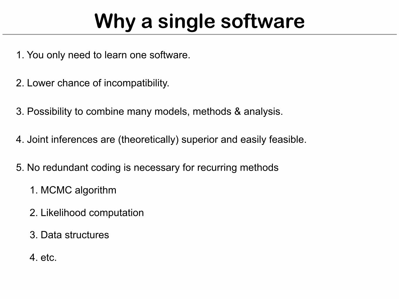
Why a single software

1. You only need to learn one software.

2. Lower chance of incompatibility.

3. Possibility to combine many models, methods & analysis.

4. Joint inferences are (theoretically) superior and easily feasible.

5. No redundant coding is necessary for recurring methods

1. MCMC algorithm

2. Likelihood computation

3. Data structures

4. etc.

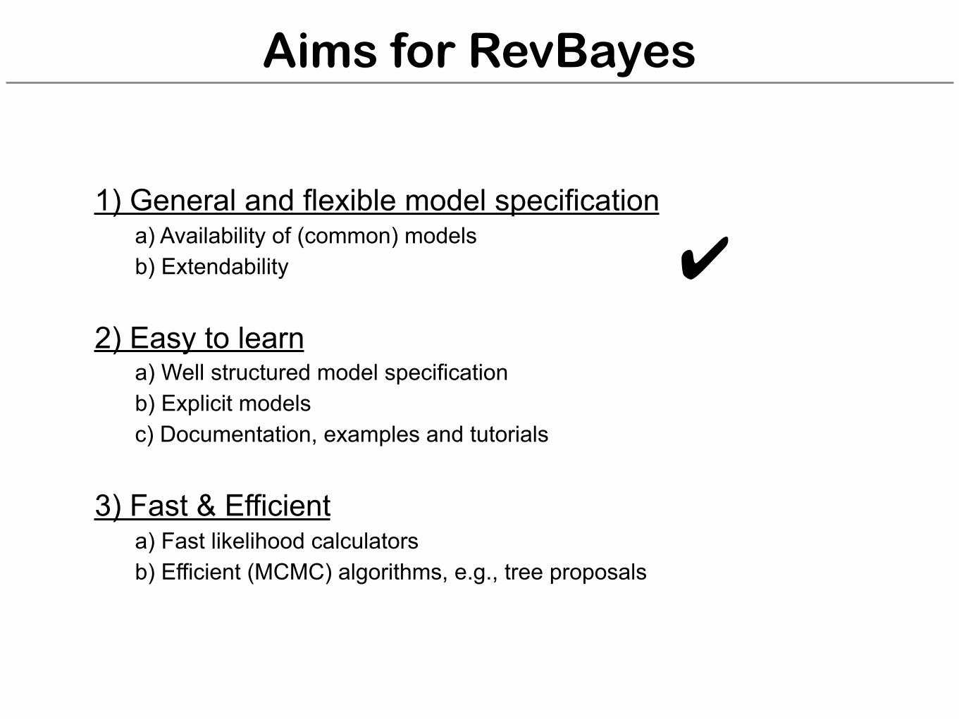
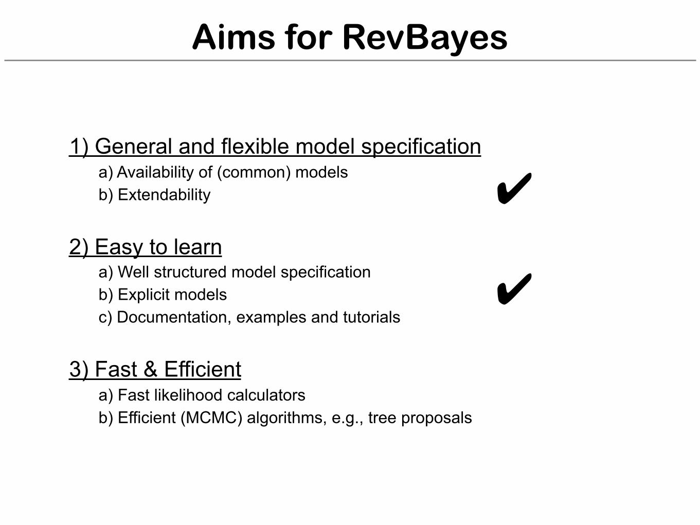
Aims for RevBayes

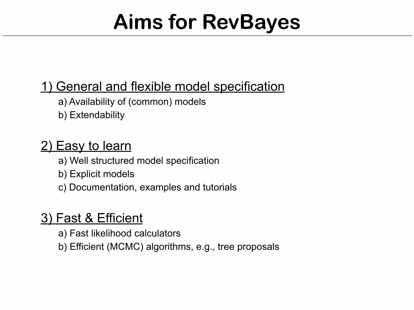
1) General and flexible model specification a) Availability of (common) models b) Extendability

2) Easy to learn a) Well structured model specification b) Explicit models c) Documentation, examples and tutorials

3) Fast & Efficient a) Fast likelihood calculators b) Efficient (MCMC) algorithms, e.g., tree proposals

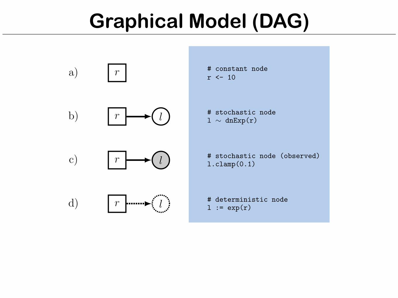
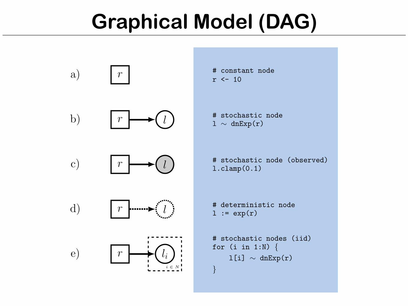
Graphical Model (DAG)

r

r

r

r

r

l

l

l

li

a)

b)

c)

d)

e)i 2 N

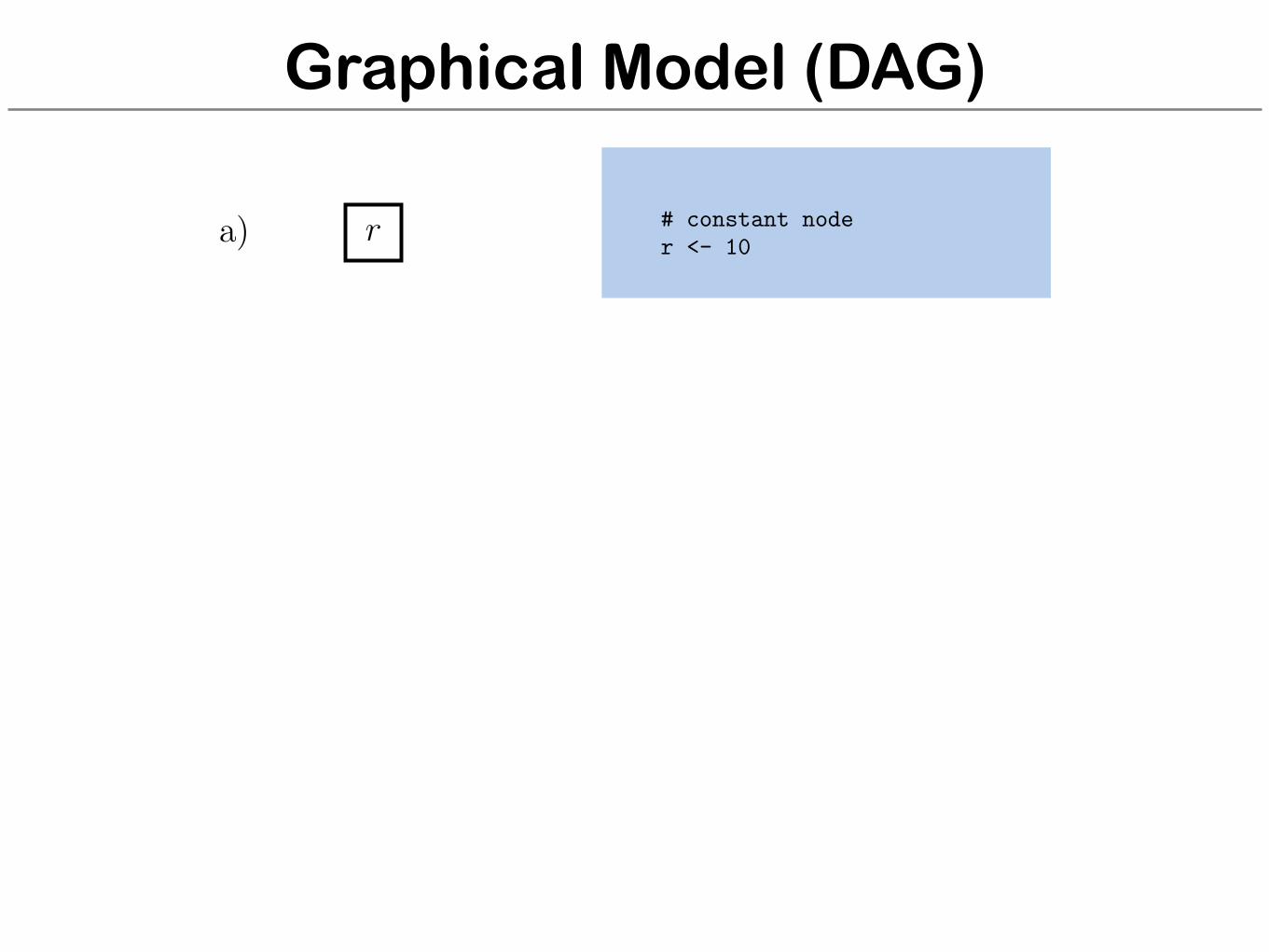
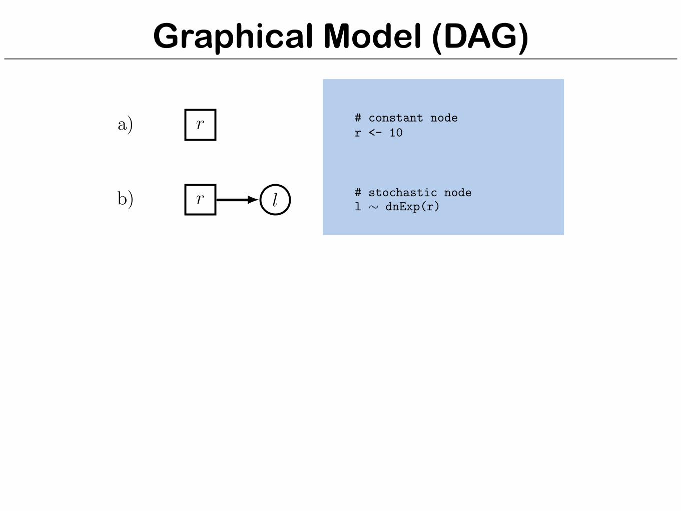
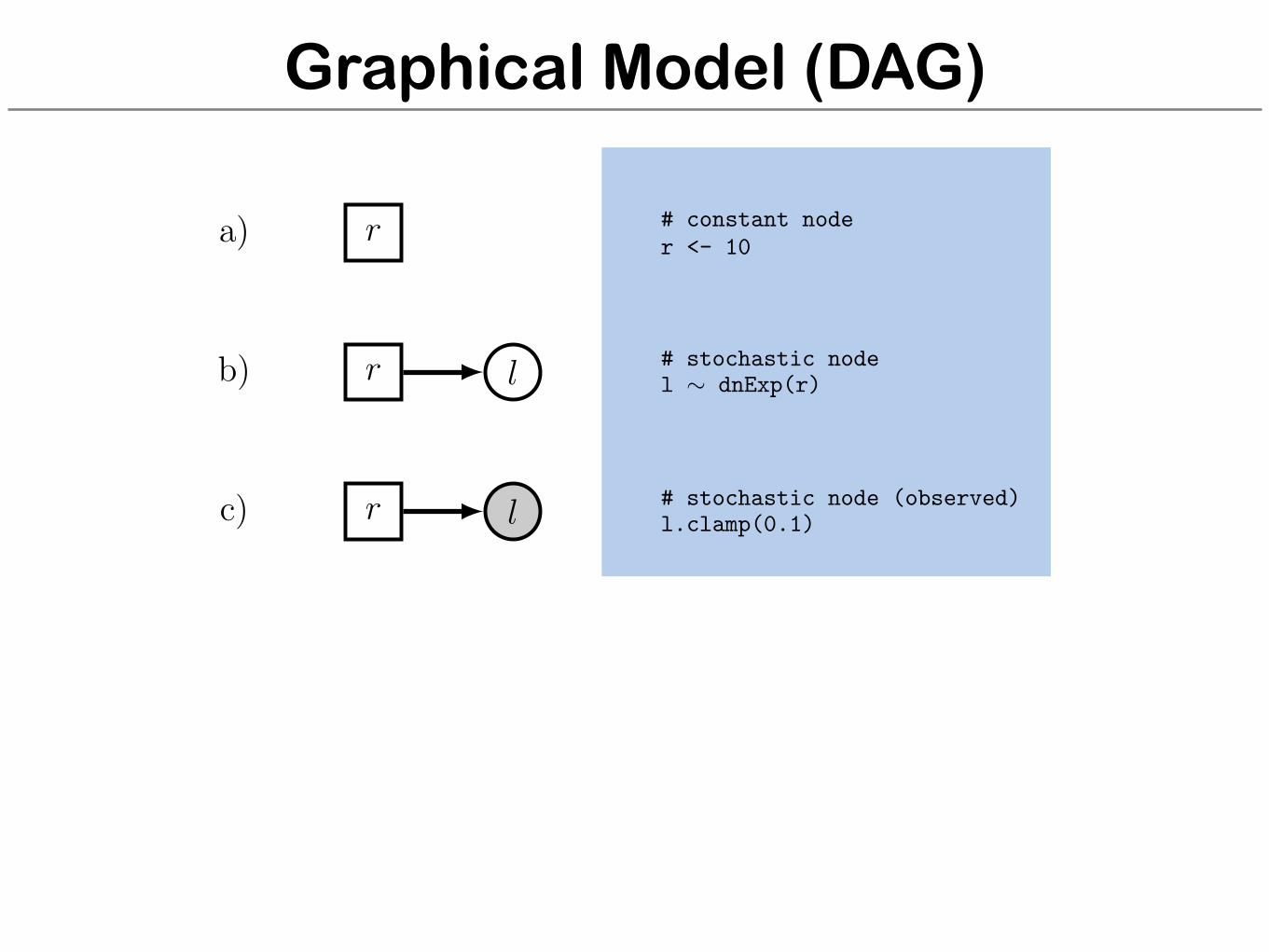
# constant noder <- 10

# stochastic nodel ⇠ dnExp(r)

# stochastic node (observed)l.clamp(0.1)

# deterministic nodel := exp(r)

# stochastic nodes (iid)for (i in 1:N) {

l[i] ⇠ dnExp(r)

}


r

r

r

r

r

l

l

l

li

a)

b)

c)

d)

e)i 2 N






l[i] ⇠ dnExp(r)

}


r

r

r

r

r

l

l

l

li

a)

b)

c)

d)

e)i 2 N






l[i] ⇠ dnExp(r)

}


r

r

r

r

r

l

l

l

li

a)

b)

c)

d)

e)i 2 N






l[i] ⇠ dnExp(r)

}


r

r

r

r

r

l

l

l

li

a)

b)

c)

d)

e)i 2 N






l[i] ⇠ dnExp(r)

}

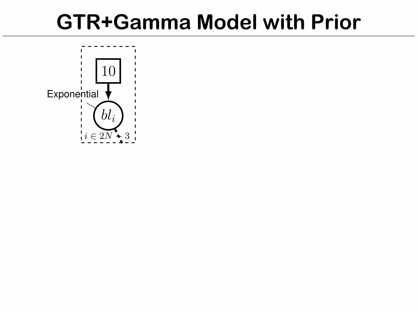
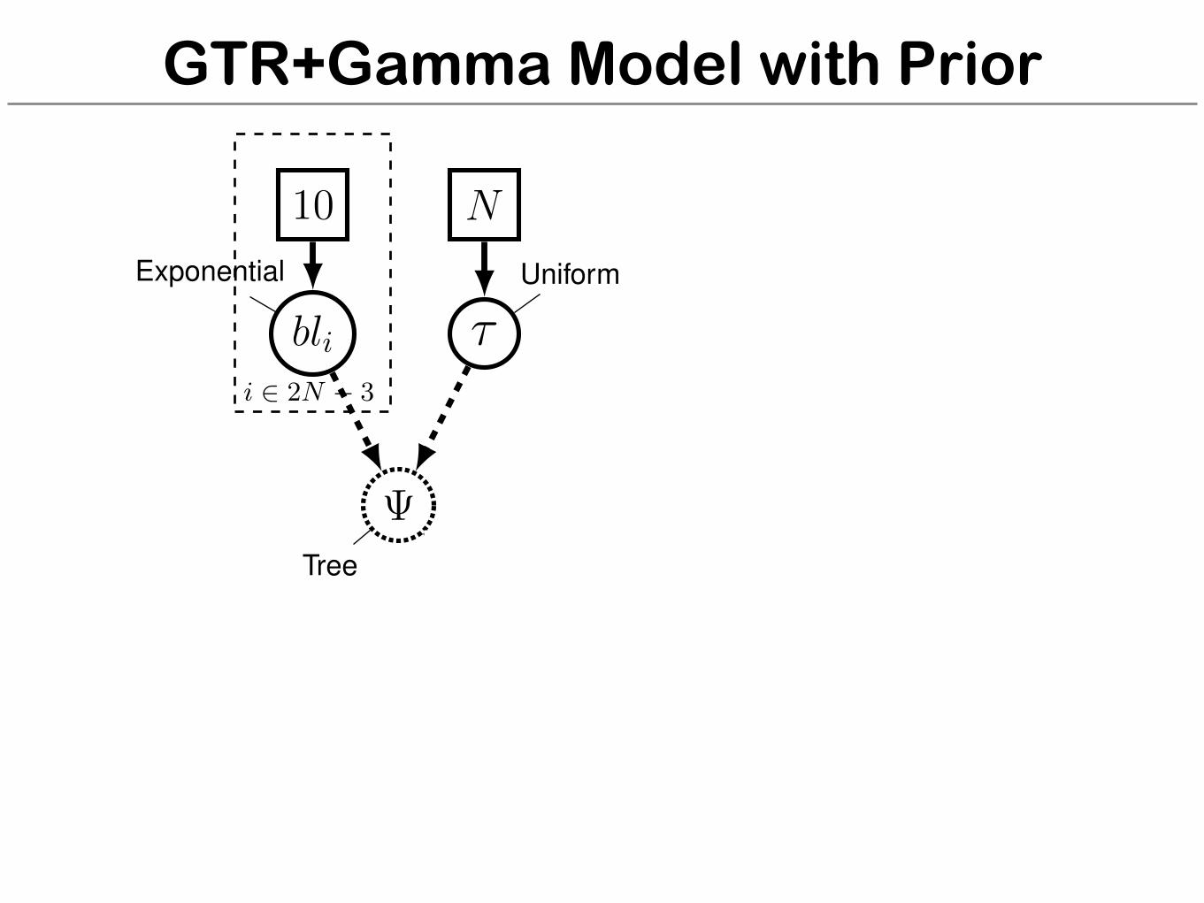
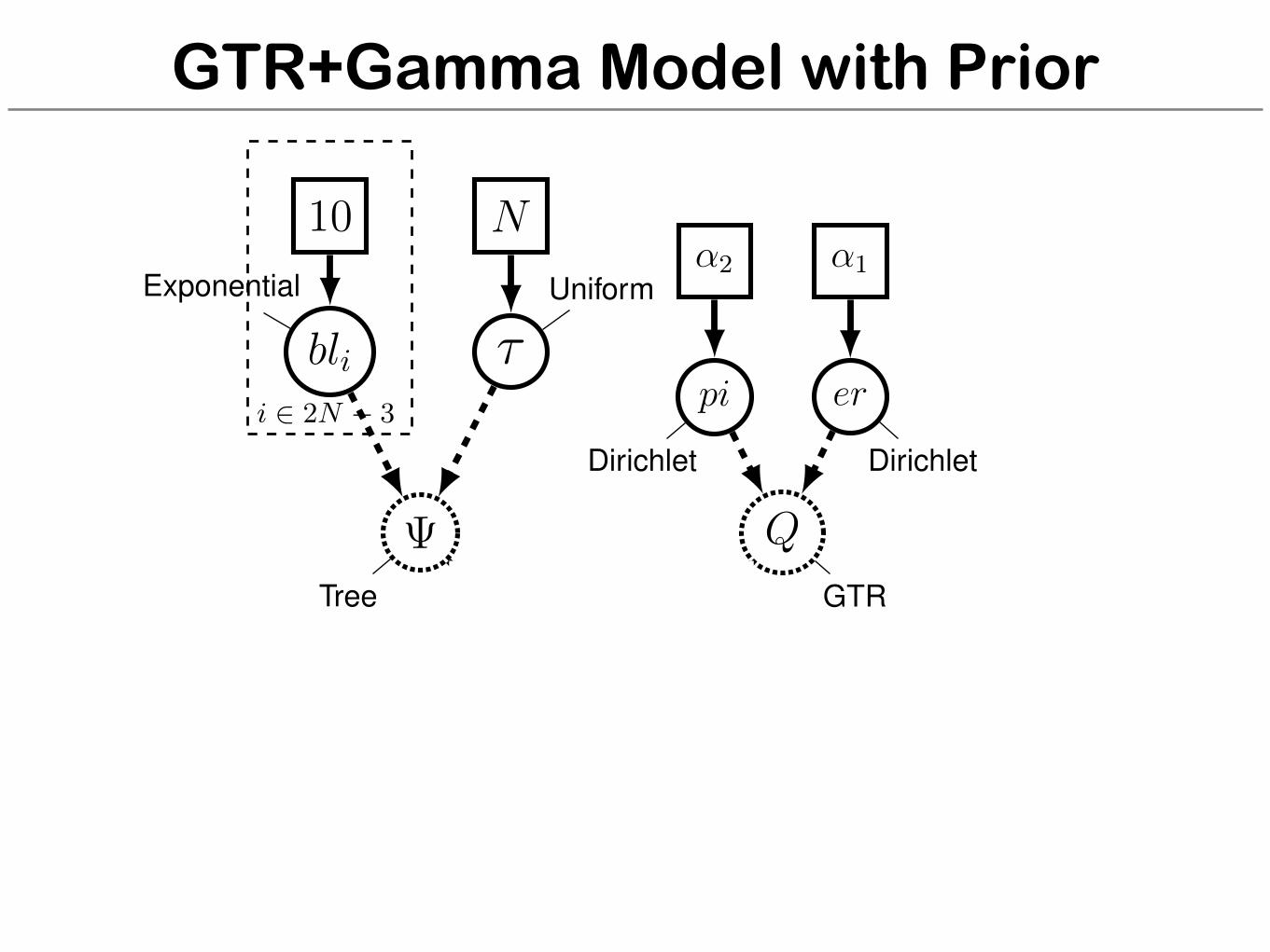
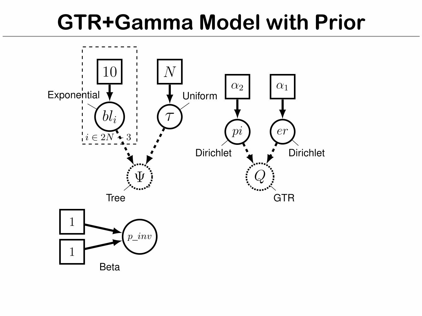
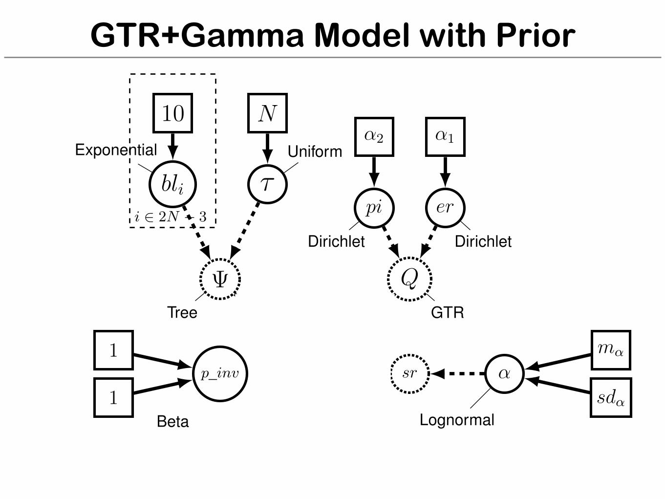
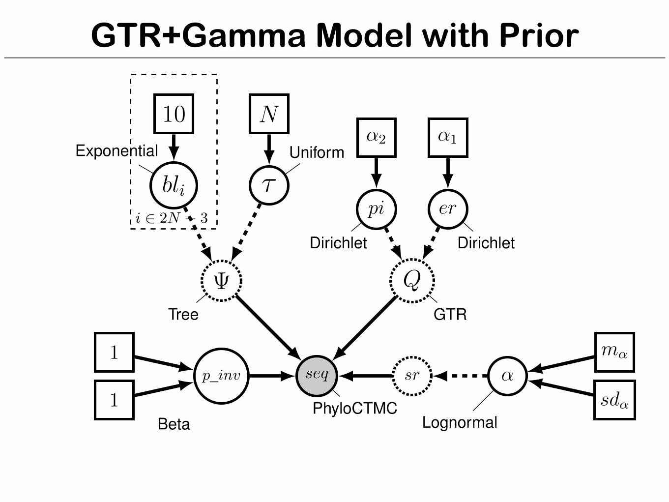
GTR+Gamma Model with Prior

seq

PhyloCTMC

Q

GTR

p_inv1

1Beta

sr ↵m↵

sd↵Lognormal

Tree

bli ⌧Exponential Uniform

10 N

i 2 2N � 3pi

Dirichlet

er

Dirichlet

↵2 ↵1

for (i in 1:n_branches) {bl[i] ⇠ dnExponential(10.0)

}topology ⇠ dnUniformTopology(taxa)psi := treeAssembly(topology, bl)

alpha1 <- v(1,1,1,1,1,1)alpha2 <- v(1,1,1,1)er ⇠ dnDirichlet( alpha1 )pi ⇠ dnDirichlet( alpha2 )Q := fnGTR(er, pi)m_alpha <- ln(5.0)sd_alpha <- 0.587405alpha ⇠ dnLognormal( m_alpha, sd_alpha )sr := fnDiscretizeGamma( alpha, alpha, 4, false )

p_inv ⇠ dnBeta(1,1)

seq ⇠ dnPhyloCTMC( tree=psi, Q=Q, pInv=p_invar,siteRates=sr, type="DNA" )

seq.clamp( data )


seq

PhyloCTMC

Q

GTR

p_inv1

1Beta

sr ↵m↵

sd↵Lognormal

Tree


10 N

i 2 2N � 3pi

Dirichlet

er

Dirichlet

↵2 ↵1






seq.clamp( data )


seq

PhyloCTMC

Q

GTR

p_inv1

1Beta

sr ↵m↵

sd↵Lognormal

Tree


10 N

i 2 2N � 3pi

Dirichlet

er

Dirichlet

↵2 ↵1






seq.clamp( data )


seq

PhyloCTMC

Q

GTR

p_inv1

1Beta

sr ↵m↵

sd↵Lognormal

Tree


10 N

i 2 2N � 3pi

Dirichlet

er

Dirichlet

↵2 ↵1






seq.clamp( data )


seq

PhyloCTMC

Q

GTR

p_inv1

1Beta

sr ↵m↵

sd↵Lognormal

Tree


10 N

i 2 2N � 3pi

Dirichlet

er

Dirichlet

↵2 ↵1






seq.clamp( data )


seq

PhyloCTMC

Q

GTR

p_inv1

1Beta

sr ↵m↵

sd↵Lognormal

Tree


10 N

i 2 2N � 3pi

Dirichlet

er

Dirichlet

↵2 ↵1






seq.clamp( data )


seq

PhyloCTMC

Q

GTR

p_inv1

1Beta

sr ↵m↵

sd↵Lognormal

Tree


10 N

i 2 2N � 3pi

Dirichlet

er

Dirichlet

↵2 ↵1






seq.clamp( data )

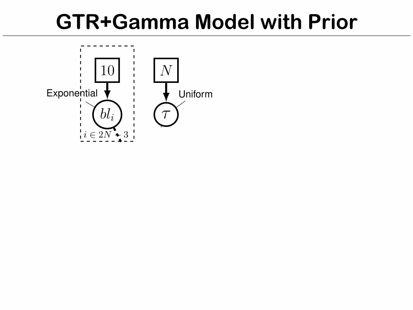
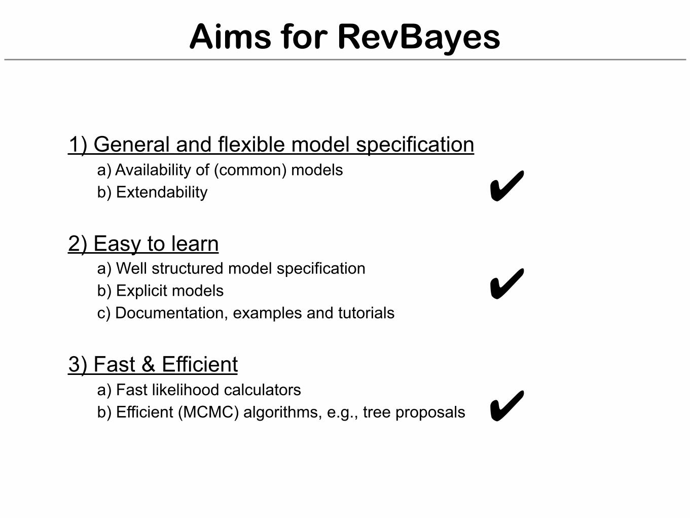
Aims for RevBayes




✔

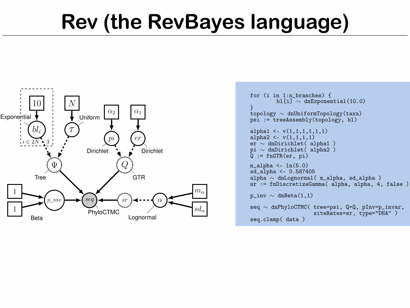
Rev (the RevBayes language)

seq

PhyloCTMC

Q

GTR

p_inv1

1Beta

sr ↵m↵

sd↵Lognormal

Tree


10 N

i 2 2N � 3pi

Dirichlet

er

Dirichlet

↵2 ↵1






seq.clamp( data )

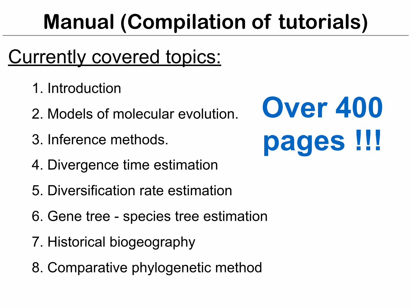
Manual (Compilation of tutorials)

1. Introduction

2. Models of molecular evolution.

3. Inference methods.

4. Divergence time estimation

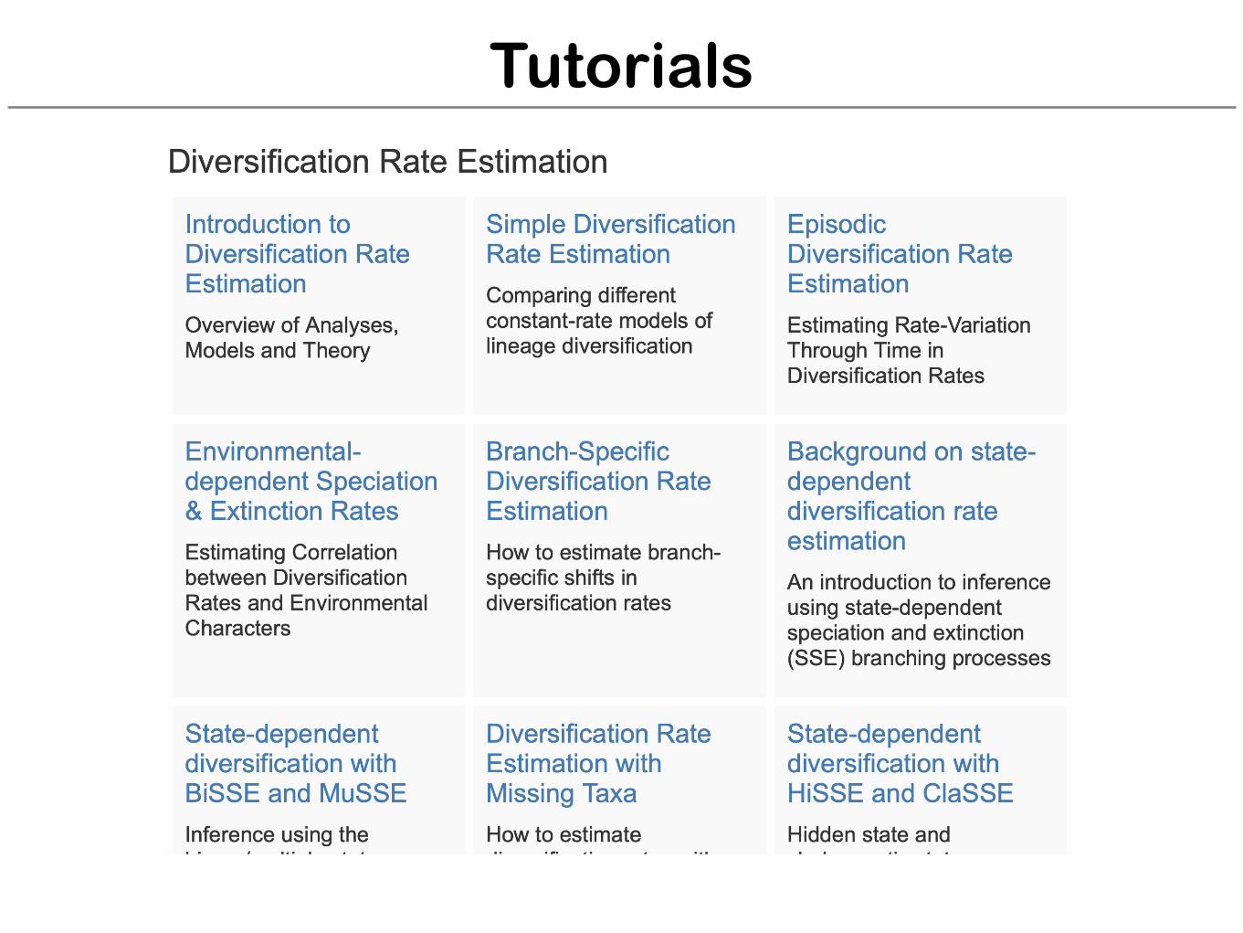
5. Diversification rate estimation

6. Gene tree - species tree estimation

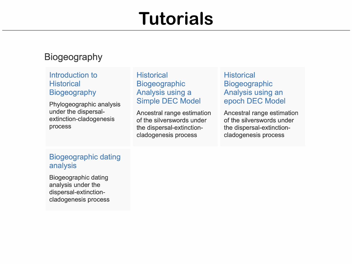
7. Historical biogeography

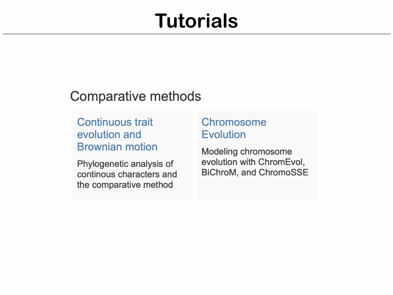
8. Comparative phylogenetic method

Over 400 pages !!!

Currently covered topics:

Aims for RevBayes




✔

✔

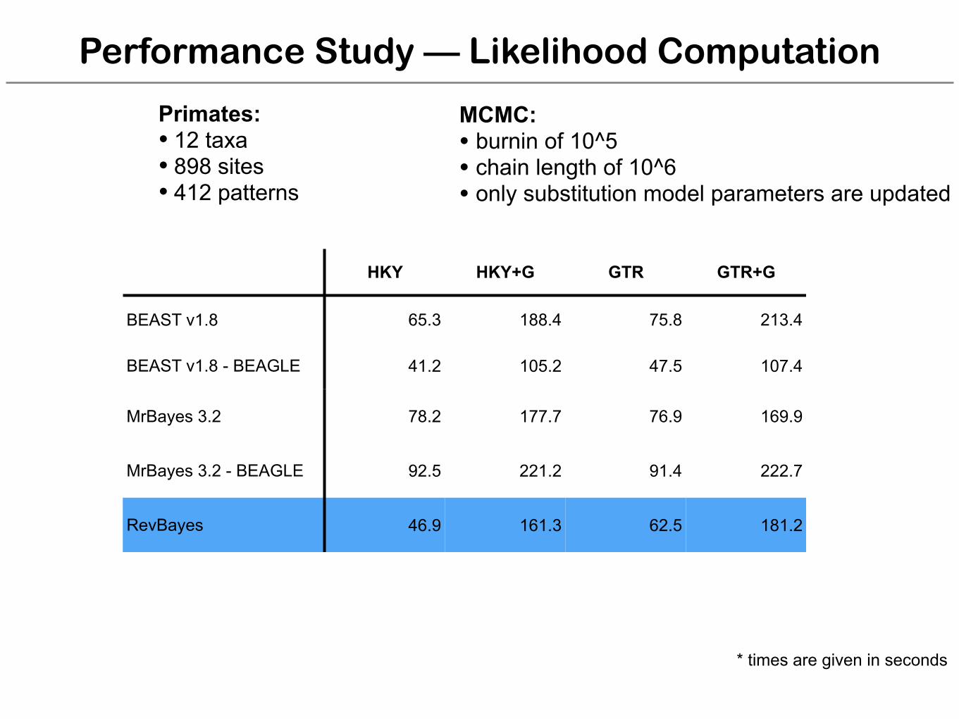
Performance Study — Likelihood Computation

HKY HKY+G GTR GTR+G

BEAST v1.8 65.3 188.4 75.8 213.4

BEAST v1.8 - BEAGLE 41.2 105.2 47.5 107.4

MrBayes 3.2 78.2 177.7 76.9 169.9

MrBayes 3.2 - BEAGLE 92.5 221.2 91.4 222.7

RevBayes 46.9 161.3 62.5 181.2

Primates: • 12 taxa • 898 sites • 412 patterns

MCMC: • burnin of 10^5 • chain length of 10^6 • only substitution model parameters are updated

* times are given in seconds

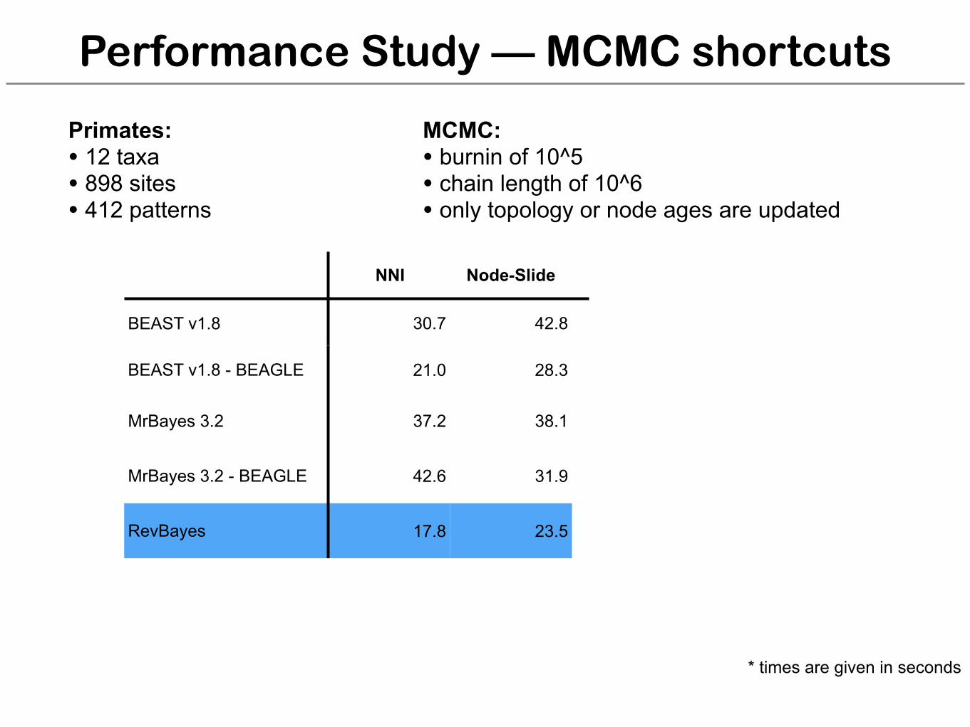
Performance Study — MCMC shortcuts

NNI Node-Slide NNI Node-Slide

BEAST v1.8 30.7 42.8

BEAST v1.8 - BEAGLE 21.0 28.3

MrBayes 3.2 37.2 38.1

MrBayes 3.2 - BEAGLE 42.6 31.9

RevBayes 17.8 23.5

* times are given in seconds

Cetaceans

Primates: • 12 taxa • 898 sites • 412 patterns

MCMC: • burnin of 10^5 • chain length of 10^6 • only topology or node ages are updated

Cetaceans: • 71 taxa• 1140 sites• 578 patterns

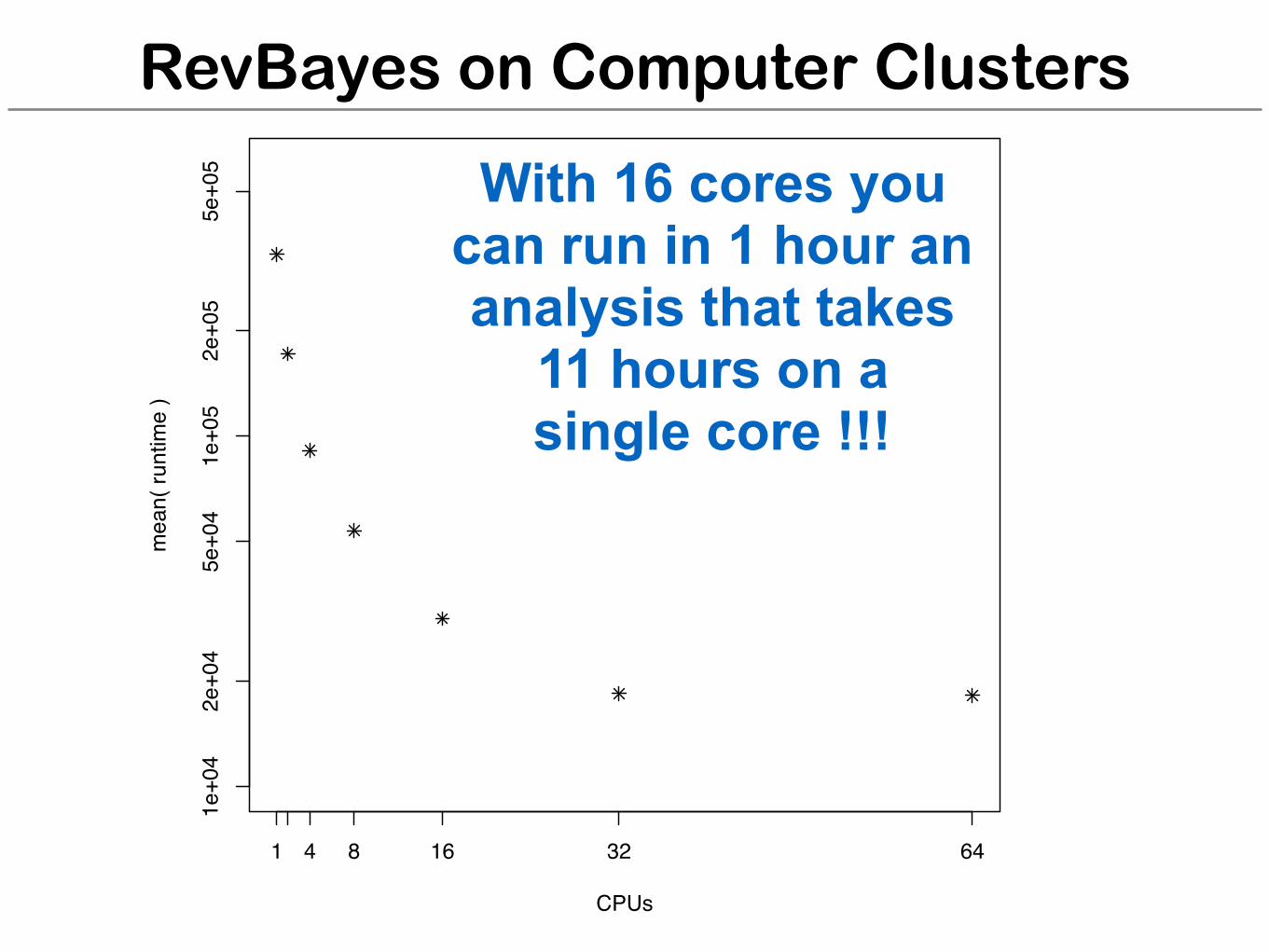
RevBayes on Computer Clusters

1e+0

42e

+04

5e+0

41e

+05

2e+0

55e

+05

CPUs

mea

n( ru

ntim

e )

1 4 8 16 32 64

With 16 cores you can run in 1 hour an analysis that takes

11 hours on a single core !!!

Aims for RevBayes




✔

✔

✔

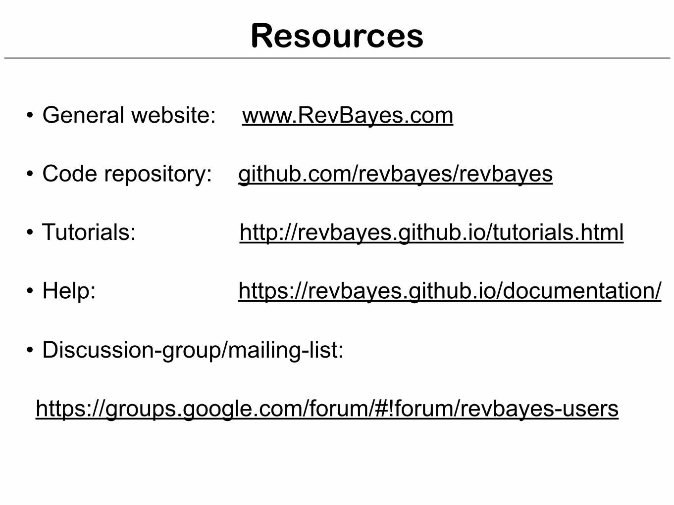
Resources

• General website: www.RevBayes.com

• Code repository: github.com/revbayes/revbayes

• Tutorials: http://revbayes.github.io/tutorials.html

• Help: https://revbayes.github.io/documentation/

• Discussion-group/mailing-list:

https://groups.google.com/forum/#!forum/revbayes-users

http://www.RevBayes.com

http://github.com/revbayes/revbayes

http://revbayes.github.io/tutorials.html

https://revbayes.github.io/documentation/

https://groups.google.com/forum/#!forum/revbayes-users

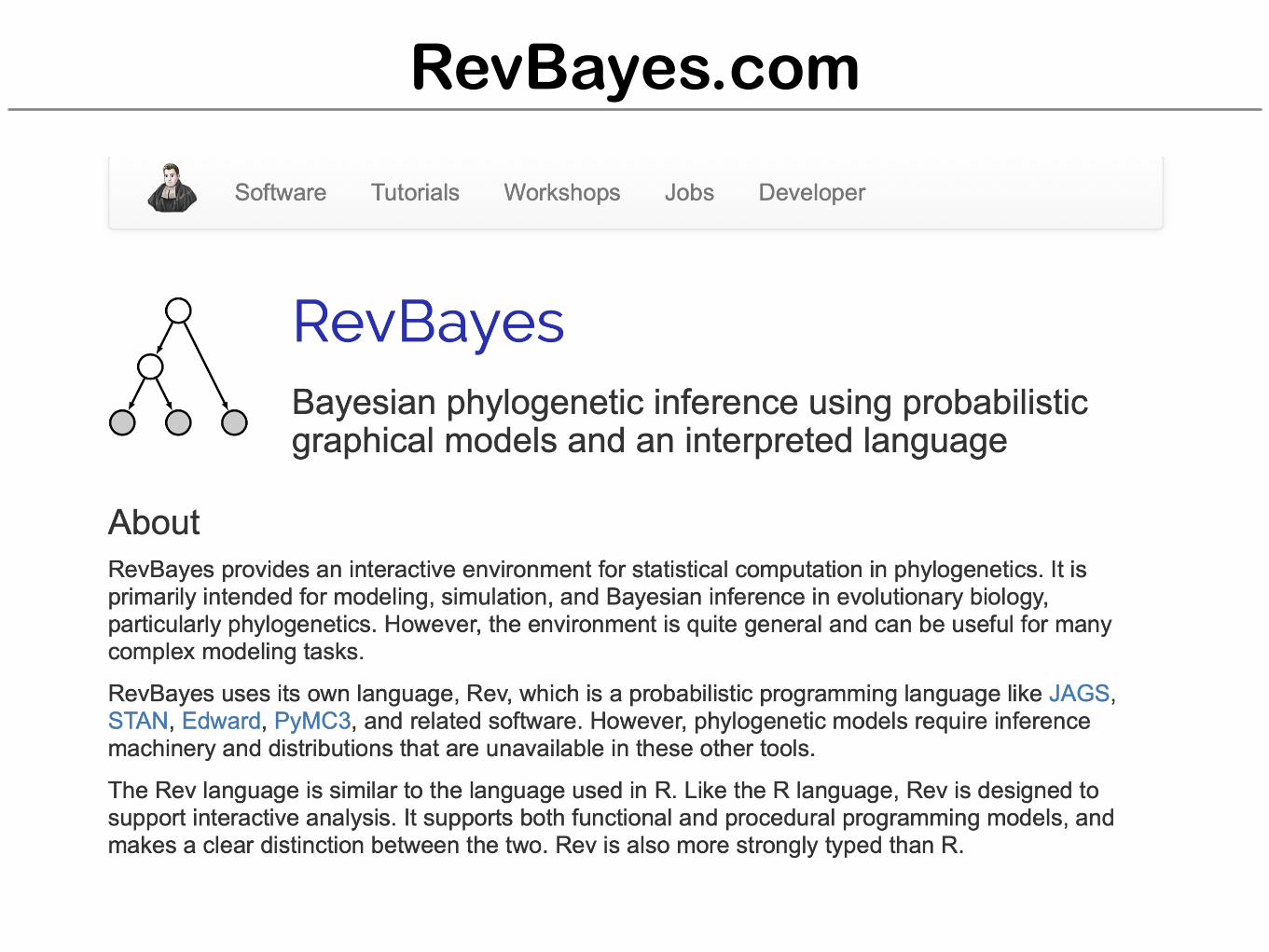
RevBayes.com

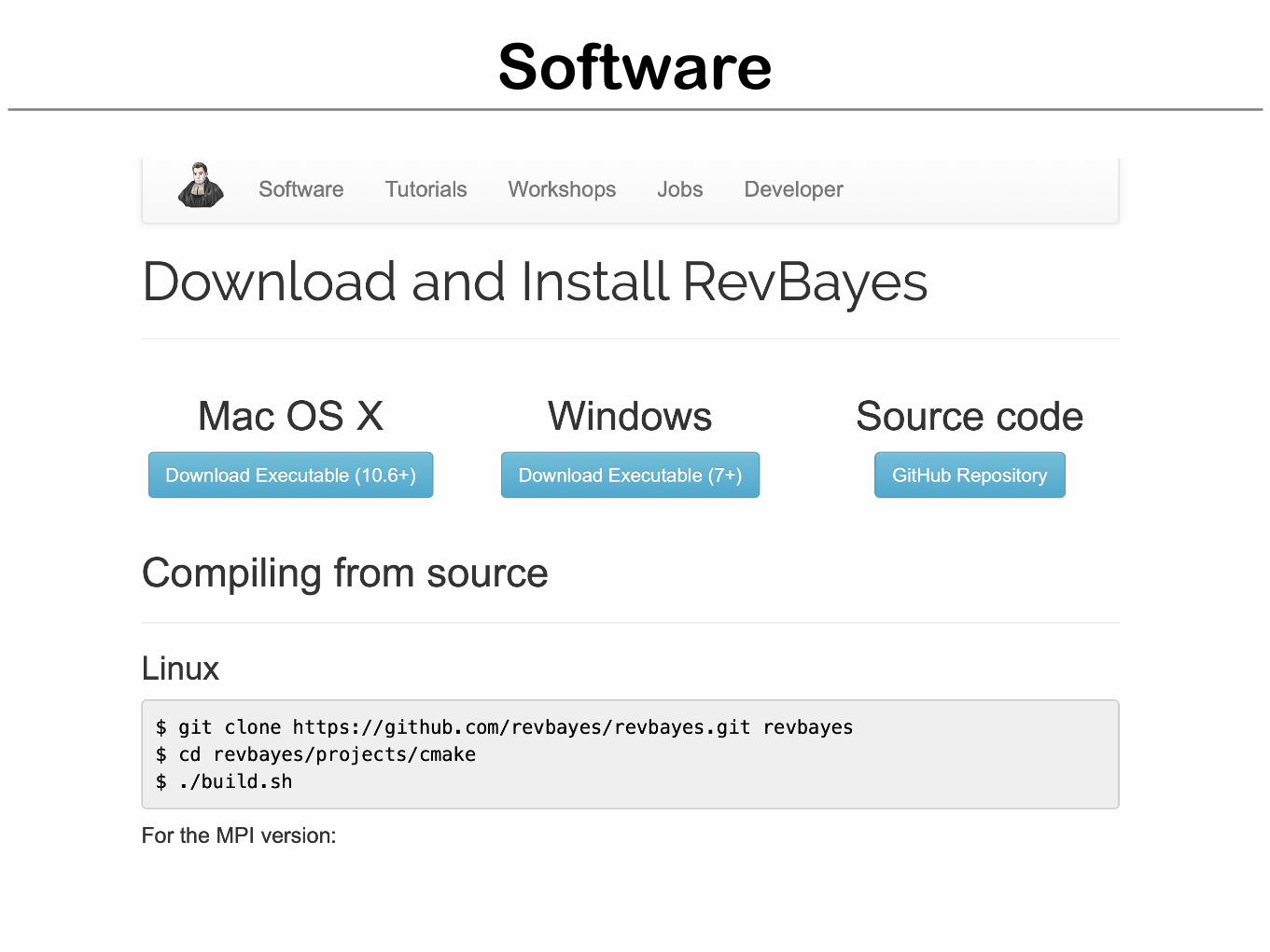
Software

Tutorials

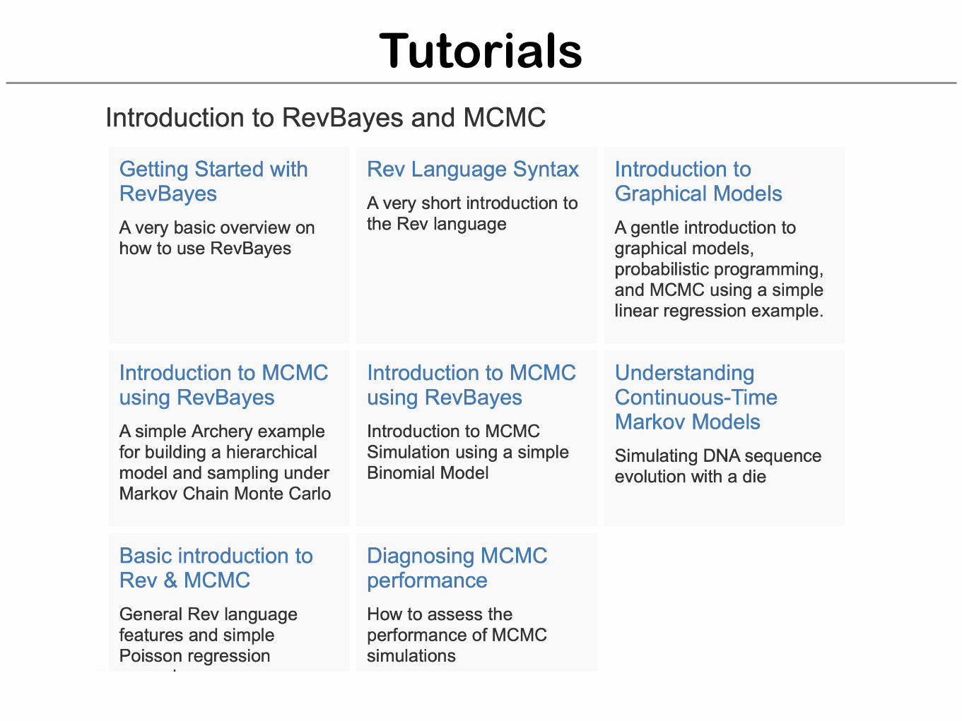
Tutorials

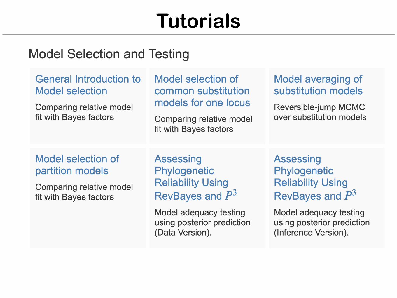
Tutorials

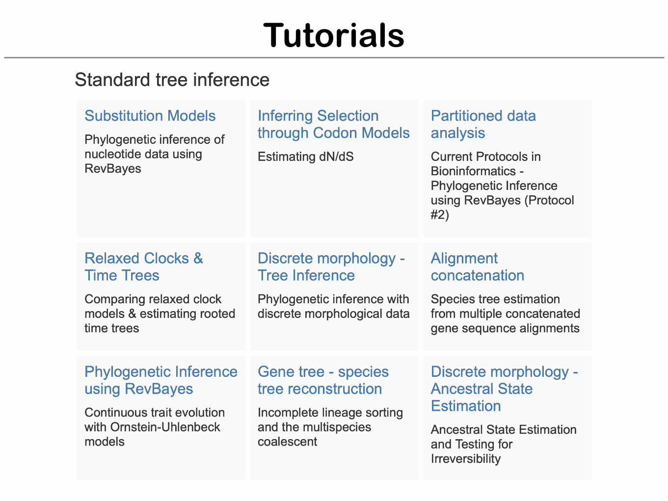
Tutorials

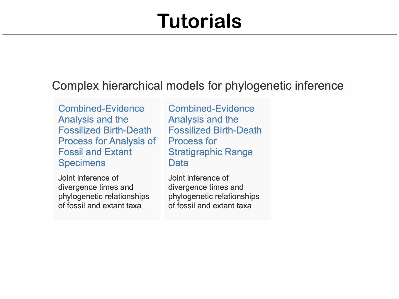
Tutorials

Tutorials

Tutorials

Tutorials

Forum/Mailing group

Documents

Bayesian Phylogenetic Inference using RevBayestreethinkers.org/wp-content/uploads/2019/05/1_RevBayes.pdf · Bayesian Phylogenetic Inference using RevBayes: Introduction to RevBayes