Embed Size (px)
Citation preview

1
Bayesian Networks:Independencies and Inference
Scott Davies and Andrew Moore
Note to other teachers and users of these slides. Andrew and Scott would be delighted if you found this source material useful in giving your own lectures. Feel free to use these slides verbatim, or to modify them to fit your own needs. PowerPoint originals are available. If you make use of a significant portion of these slides in your own lecture, please include this message, or the following link to the source repository of Andrew’s tutorials: http://www.cs.cmu.edu/~awm/tutorials . Comments and corrections gratefully received.

2
What Independencies does a Bayes Net Model?
• In order for a Bayesian network to model a probability distribution, the following must be true by definition:
Each variable is conditionally independent of all its non-descendants in the graph given the value of all its parents.
• This implies
• But what else does it imply?
∏=
=n
iiin XparentsXPXXP
11 ))(|()( K

3
What Independencies does a Bayes Net Model?
• Example:
Z
Y
X
Given Y, does learning the value of Z tell usnothing new about X?
I.e., is P(X|Y, Z) equal to P(X | Y)?
Yes. Since we know the value of all of X’s parents (namely, Y), and Z is not a descendant of X, X is conditionally
independent of Z.
Also, since independence is symmetric, P(Z|Y, X) = P(Z|Y).
Quick proof that independence is symmetric
• Assume: P(X|Y, Z) = P(X|Y)• Then:
),()()|,(),|(
YXPZPZYXPYXZP =
)()|()(),|()|(
YPYXPZPZYXPZYP
=
(Bayes’s Rule)
(Chain Rule)
(By Assumption)
(Bayes’s Rule)
)()|()()|()|(
YPYXPZPYXPZYP
=
)|()(
)()|( YZPYP
ZPZYP==

4
What Independencies does a Bayes Net Model?
• Let I<X,Y,Z> represent X and Z being conditionally independent given Y.
• I<X,Y,Z>? Yes, just as in previous example: All X’s parents given, and Z is not a descendant.
Y
X Z
What Independencies does a Bayes Net Model?
• I<X,{U},Z>? No.• I<X,{U,V},Z>? Yes.• Maybe I<X, S, Z> iff S acts a cutset between X and Z
in an undirected version of the graph…?
Z
VU
X

5
Things get a little more confusing
• X has no parents, so we’re know all its parents’values trivially
• Z is not a descendant of X• So, I<X,{},Z>, even though there’s a undirected path
from X to Z through an unknown variable Y.• What if we do know the value of Y, though? Or one
of its descendants?
ZX
Y
The “Burglar Alarm” example
• Your house has a twitchy burglar alarm that is also sometimes triggered by earthquakes.
• Earth arguably doesn’t care whether your house is currently being burgled
• While you are on vacation, one of your neighbors calls and tells you your home’s burglar alarm is ringing. Uh oh!
Burglar Earthquake
Alarm
Phone Call

6
Things get a lot more confusing
• But now suppose you learn that there was a medium-sized earthquake in your neighborhood. Oh, whew! Probably not a burglar after all.
• Earthquake “explains away” the hypothetical burglar.• But then it must not be the case that
I<Burglar,{Phone Call}, Earthquake>, even thoughI<Burglar,{}, Earthquake>!
Burglar Earthquake
Alarm
Phone Call
d-separation to the rescue
• Fortunately, there is a relatively simple algorithm for determining whether two variables in a Bayesian network are conditionally independent: d-separation.
• Definition: X and Z are d-separated by a set of evidence variables E iff every undirected path from Xto Z is “blocked”, where a path is “blocked” iff one or more of the following conditions is true: ...

7
A path is “blocked” when...
• There exists a variable V on the path such that• it is in the evidence set E• the arcs putting V in the path are “tail-to-tail”
• Or, there exists a variable V on the path such that• it is in the evidence set E• the arcs putting V in the path are “tail-to-head”
• Or, ...
V
V
A path is “blocked” when… (the funky case)
• … Or, there exists a variable V on the path such that• it is NOT in the evidence set E• neither are any of its descendants• the arcs putting V on the path are “head-to-head”
V

8
d-separation to the rescue, cont’d
• Theorem [Verma & Pearl, 1998]:• If a set of evidence variables E d-separates X and
Z in a Bayesian network’s graph, then I<X, E, Z>.• d-separation can be computed in linear time using a
depth-first-search-like algorithm.• Great! We now have a fast algorithm for
automatically inferring whether learning the value of one variable might give us any additional hints about some other variable, given what we already know. • “Might”: Variables may actually be independent when they’re not d-
separated, depending on the actual probabilities involved
d-separation example
A B
C D
E F
G
I
H
J
•I<C, {}, D>?•I<C, {A}, D>?•I<C, {A, B}, D>?•I<C, {A, B, J}, D>?•I<C, {A, B, E, J}, D>?

9
Bayesian Network Inference
• Inference: calculating P(X|Y) for some variables or sets of variables X and Y.
• Inference in Bayesian networks is #P-hard!
Reduces to
How many satisfying assignments?
I1 I2 I3 I4 I5
O
Inputs: prior probabilities of .5
P(O) must be(#sat. assign.)*(.5^#inputs)
Bayesian Network Inference
• But…inference is still tractable in some cases.• Let’s look a special class of networks: trees / forests
in which each node has at most one parent.

10
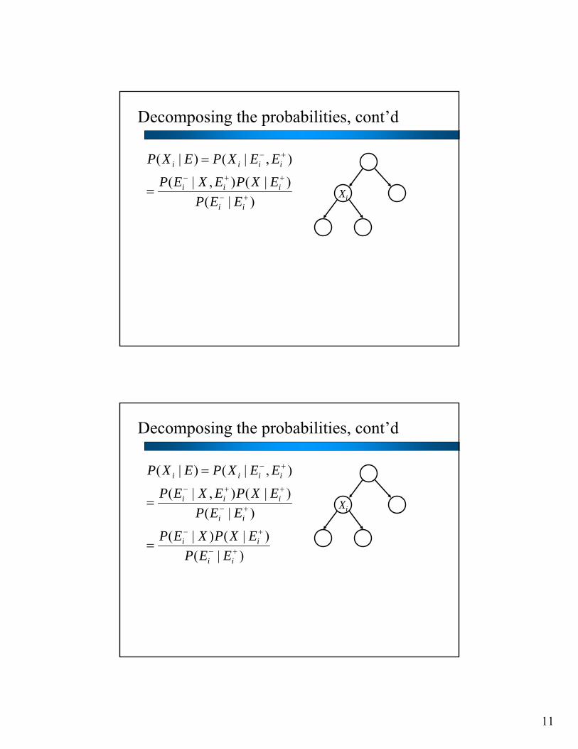
Decomposing the probabilities
• Suppose we want P(Xi | E) where E is some set of evidence variables.
• Let’s split E into two parts:• Ei
- is the part consisting of assignments to variables in the subtree rooted at Xi
• Ei+ is the rest of it
Xi
Decomposing the probabilities, cont’d
),|()|( +−= iiii EEXPEXP
Xi
11
Decomposing the probabilities, cont’d
)|()|(),|(
),|()|(
+−
++−
+−
=
=
ii
iii
iiii
EEPEXPEXEP
EEXPEXP
Xi
Decomposing the probabilities, cont’d
)|()|()|(
)|()|(),|(
),|()|(
+−
+−
+−
++−
+−
=
=
=
ii
ii
ii
iii
iiii
EEPEXPXEP
EEPEXPEXEP
EEXPEXP
Xi

12
Decomposing the probabilities, cont’d
)(λ)(απ)|(
)|()|(
)|()|(),|(
),|()|(
ii
ii
ii
ii
iii
iiii
XXEEP
EXPXEP
EEPEXPEXEP
EEXPEXP
=
=
=
=
+−
+−
+−
++−
+−
Xi
Where:• α is a constant independent of Xi• π(Xi) = P(Xi |Ei
+)• λ(Xi) = P(Ei
-| Xi)
Using the decomposition for inference
• We can use this decomposition to do inference as follows. First, compute λ(Xi) = P(Ei
-| Xi) for all Xirecursively, using the leaves of the tree as the base case.
• If Xi is a leaf:• If Xi is in E: λ(Xi) = 1 if Xi matches E, 0 otherwise• If Xi is not in E: Ei
- is the null set, so P(Ei
-| Xi) = 1 (constant)

13
Quick aside: “Virtual evidence”
• For theoretical simplicity, but without loss of generality, let’s assume that all variables in E (the evidence set) are leaves in the tree.
• Why can we do this WLOG:
XiXi
Xi’Observe Xi
Equivalent to
Observe Xi’
Where P(Xi’| Xi) =1 if Xi’=Xi, 0 otherwise
Calculating λ(Xi) for non-leaves
• Suppose Xi has one child, Xc.
• Then:
Xi
Xc
== − )|()(λ iii XEPX

14
Calculating λ(Xi) for non-leaves
• Suppose Xi has one child, Xc.
• Then:
Xi
Xc
∑ === −−
jiCiiii XjXEPXEPX )|,()|()(λ
Calculating λ(Xi) for non-leaves
• Suppose Xi has one child, Xc.
• Then:
Xi
Xc
∑
∑===
===
−
−−
jCiiiC
jiCiiii
jXXEPXjXP
XjXEPXEPX
),|()|(
)|,()|()(λ

15
Calculating λ(Xi) for non-leaves
• Suppose Xi has one child, Xc.
• Then:
Xi
Xc
∑
∑
∑
∑
===
===
===
===
−
−
−−
jCiC
jCiiC
jCiiiC
jiCiiii
jXXjXP
jXEPXjXP
jXXEPXjXP
XjXEPXEPX
)(λ)|(
)|()|(
),|()|(
)|,()|()(λ
Calculating λ(Xi) for non-leaves
• Now, suppose Xi has a set of children, C.• Since Xi d-separates each of its subtrees, the
contribution of each subtree to λ(Xi) is independent:
∏ ∑
∏
∈
∈
−
⎥⎥⎦
⎤
⎢⎢⎣
⎡=
==
CX Xjij
CXijiii
j j
j
XXXP
XXEPX
)λ()|(
)(λ)|()(λ
where λj(Xi) is the contribution to P(Ei-| Xi) of the part of
the evidence lying in the subtree rooted at one of Xi’schildren Xj.

16
We are now λ-happy
• So now we have a way to recursively compute all the λ(Xi)’s, starting from the root and using the leaves as the base case.
• If we want, we can think of each node in the network as an autonomous processor that passes a little “λmessage” to its parent.
λ λ λ λ
λλ
The other half of the problem
• Remember, P(Xi|E) = απ(Xi)λ(Xi). Now that we have all the λ(Xi)’s, what about the π(Xi)’s?
π(Xi) = P(Xi |Ei+).
• What about the root of the tree, Xr? In that case, Er+
is the null set, so π(Xr) = P(Xr). No sweat. Since we also know λ(Xr), we can compute the final P(Xr).
• So for an arbitrary Xi with parent Xp, let’s inductively assume we know π(Xp) and/or P(Xp|E). How do we get π(Xi)?

17
Computing π(Xi)
Xp
Xi
== + )|()(π iii EXPX
Computing π(Xi)
Xp
Xi
∑ ++ ===j
ipiiii EjXXPEXPX )|,()|()(π

18
Computing π(Xi)
Xp
Xi
∑
∑++
++
===
===
jipipi
jipiiii
EjXPEjXXP
EjXXPEXPX
)|(),|(
)|,()|()(π
Computing π(Xi)
Xp
Xi
∑
∑
∑
+
++
++
===
===
===
jippi
jipipi
jipiiii
EjXPjXXP
EjXPEjXXP
EjXXPEXPX
)|()|(
)|(),|(
)|,()|()(π

19
Computing π(Xi)
Xp
Xi
∑
∑
∑
∑
=
===
===
===
===
+
++
++
j pi
ppi
jippi
jipipi
jipiiii
jXEjXP
jXXP
EjXPjXXP
EjXPEjXXP
EjXXPEXPX
)(λ)|(
)|(
)|()|(
)|(),|(
)|,()|()(π
Computing π(Xi)
Xp
Xi
Where πi(Xp) is defined as
∑
∑
∑
∑
∑
===
=
===
===
===
===
+
++
++
jpipi
j pi
ppi
jippi
jipipi
jipiiii
jXjXXP
jXEjXP
jXXP
EjXPjXXP
EjXPEjXXP
EjXXPEXPX
)(π)|(
)(λ)|(
)|(
)|()|(
)|(),|(
)|,()|()(π
)(λ)|(
pi
p
XEXP

20
We’re done. Yay!
• Thus we can compute all the π(Xi)’s, and, in turn, all the P(Xi|E)’s.
• Can think of nodes as autonomous processors passing λ and π messages to their neighbors
λ λ λ λ
λλπ π
π π π π
Conjunctive queries
• What if we want, e.g., P(A, B | C) instead of just marginal distributions P(A | C) and P(B | C)?
• Just use chain rule:• P(A, B | C) = P(A | C) P(B | A, C)• Each of the latter probabilities can be computed
using the technique just discussed.
21
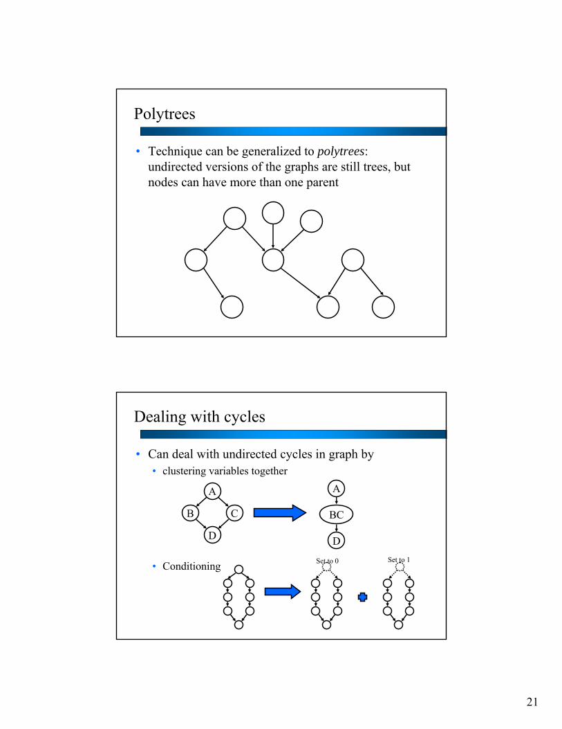
Polytrees
• Technique can be generalized to polytrees: undirected versions of the graphs are still trees, but nodes can have more than one parent
Dealing with cycles
• Can deal with undirected cycles in graph by• clustering variables together
• Conditioning
A
B C
D
A
D
BC
Set to 0 Set to 1
22
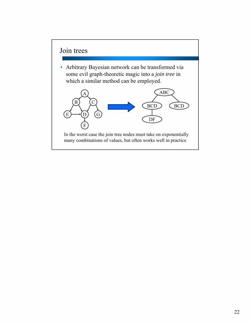
Join trees
• Arbitrary Bayesian network can be transformed via some evil graph-theoretic magic into a join tree in which a similar method can be employed.
A
B
E D
F
C
G
ABC
BCD BCD
DF
In the worst case the join tree nodes must take on exponentiallymany combinations of values, but often works well in practice