Embed Size (px)
Citation preview
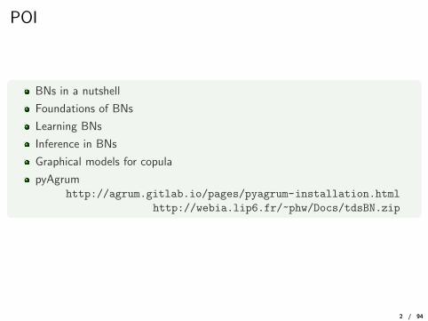
POI
BNs in a nutshell
Foundations of BNs
Learning BNs
Inference in BNs
Graphical models for copula
pyAgrumhttp://agrum.gitlab.io/pages/pyagrum-installation.html
http://webia.lip6.fr/~phw/Docs/tdsBN.zip
2 / 94
Nutshell
3 / 94
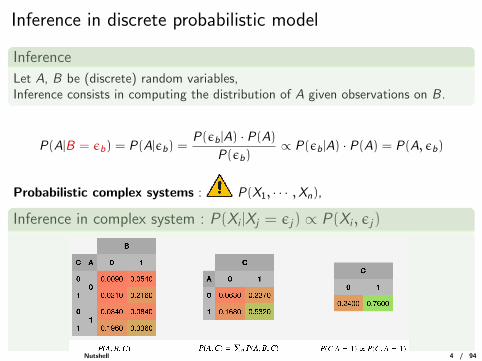
Inference in discrete probabilistic model
Inference
Let A, B be (discrete) random variables,Inference consists in computing the distribution of A given observations on B.
P(A|B = εb) = P(A|εb) =P(εb |A) · P(A)
P(εb)∝ P(εb |A) · P(A) = P(A, εb)
Probabilistic complex systems : P(X1, · · · ,Xn),
Inference in complex system : P(Xi |Xj = εj) ∝ P(Xi , εj)
P(Xi |εj) =
∑k/∈{i,j}
P(x1, · · · ,Xi , · · · , εj , · · · , xn)∑k 6=j
P(x1, · · · , xi , · · · , εj , · · · , xn)
Combinatorial explosion, curse of dimensionality !
Nutshell 4 / 94
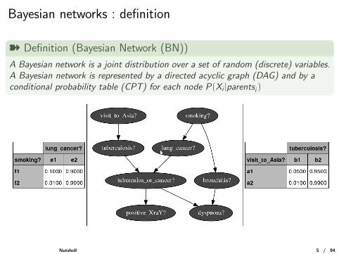
Bayesian networks : definition
ý Definition (Bayesian Network (BN))
A Bayesian network is a joint distribution over a set of random (discrete) variables.A Bayesian network is represented by a directed acyclic graph (DAG) and by aconditional probability table (CPT) for each node P(Xi |parentsi )
Nutshell 5 / 94
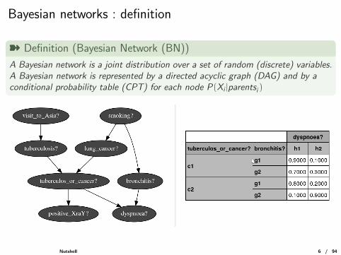
Bayesian networks : definition
ý Definition (Bayesian Network (BN))
A Bayesian network is a joint distribution over a set of random (discrete) variables.A Bayesian network is represented by a directed acyclic graph (DAG) and by aconditional probability table (CPT) for each node P(Xi |parentsi )
Nutshell 6 / 94
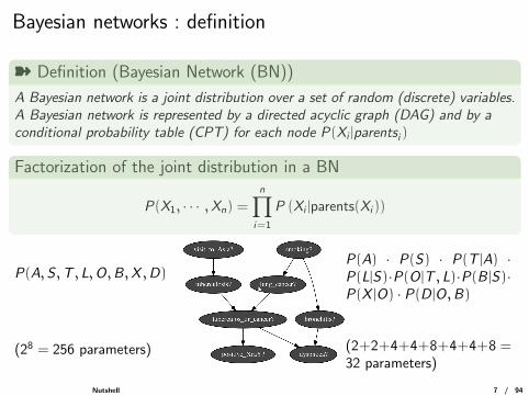
Bayesian networks : definition
ý Definition (Bayesian Network (BN))
A Bayesian network is a joint distribution over a set of random (discrete) variables.A Bayesian network is represented by a directed acyclic graph (DAG) and by aconditional probability table (CPT) for each node P(Xi |parentsi )
Factorization of the joint distribution in a BN
P(X1, · · · ,Xn) =
n∏i=1
P (Xi |parents(Xi ))
P(A,S ,T , L,O,B,X ,D)
(28 = 256 parameters)
P(A) · P(S) · P(T |A) ·P(L|S)·P(O |T , L)·P(B |S)·P(X |O) · P(D |O,B)
(2+2+4+4+8+4+4+8 =32 parameters)
Nutshell 7 / 94
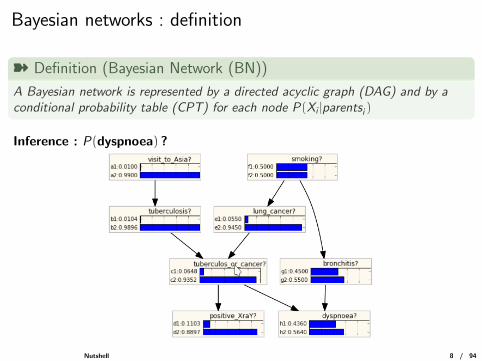
Bayesian networks : definition
ý Definition (Bayesian Network (BN))
A Bayesian network is represented by a directed acyclic graph (DAG) and by aconditional probability table (CPT) for each node P(Xi |parentsi )
Inference : P(dyspnoea) ?
Nutshell 8 / 94
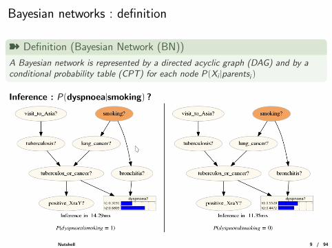
Bayesian networks : definition
ý Definition (Bayesian Network (BN))
A Bayesian network is represented by a directed acyclic graph (DAG) and by aconditional probability table (CPT) for each node P(Xi |parentsi )
Inference : P(dyspnoea|smoking) ?
Nutshell 9 / 94
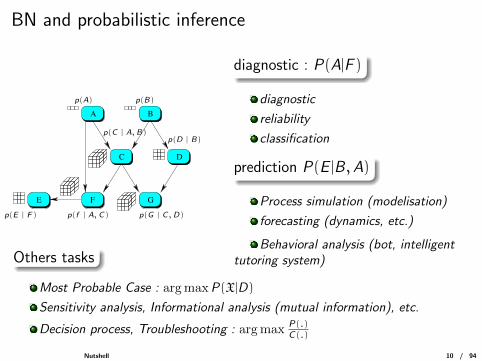
BN and probabilistic inference
A B
D
GFE
C
p(A) p(B)
p(C | A, B)p(D | B)
p(G | C ,D)p(f | A, C)p(E | F)
diagnostic : P(A|F )
diagnostic
reliability
classification
prediction P(E |B ,A)
Process simulation (modelisation)
forecasting (dynamics, etc.)
Behavioral analysis (bot, intelligenttutoring system)Others tasks
Most Probable Case : argmaxP(X|D)
Sensitivity analysis, Informational analysis (mutual information), etc.
Decision process, Troubleshooting : argmax P(.)C(.)
Nutshell 10 / 94
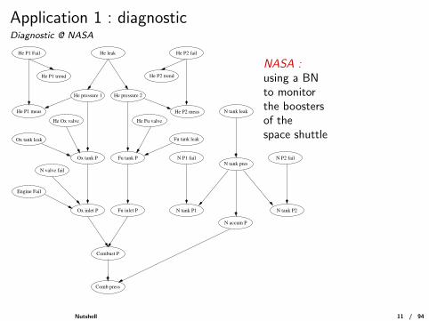
Application 1 : diagnosticDiagnostic @ NASA
NASA :using a BNto monitorthe boostersof thespace shuttle
He P1 Fail He leak
He P1 trend
He pressure 1
He P1 meas
He Ox valve
Ox tank leak
Ox tank P
He P2 fail
He pressure 2
He P2 trend
He P2 meas
Fu tank P
He Fu valve
Fu tank leak
N valve fail
Engine Fail
Ox inlet P Fu inlet P
N P1 fail
N tank P1
Combust P
Comb press
N tank leak
N tank presN P2 fail
N tank P2
N accum P
Nutshell 11 / 94

Application 2 : medical diagnosisthe Great Ormond Street hospital for sick children
Diagnosis of the causes of cyanosis or heart attack in the child just after birth.
Duct FlowLVH mixingCardiac lung
parenchyma lung flow
Hypoxiadistribution CO2
chestX−ray
reportLVH lower
body O2X−rayreport
CO2report
gruntingreport
grunting
sick
age atpresentationdisease
birthasphyxia
hypoxiain O2
right upquad O2
Nutshell 12 / 94
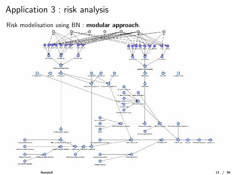
Application 3 : risk analysis
Risk modelisation using BN : modular approach.
Nutshell 13 / 94
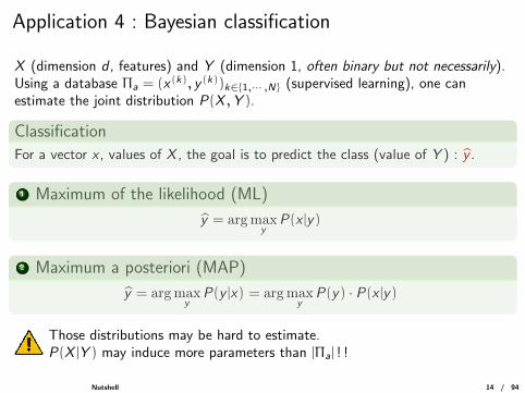
Application 4 : Bayesian classification
X (dimension d , features) and Y (dimension 1, often binary but not necessarily).Using a database Πa = (x(k), y (k))k∈{1,··· ,N} (supervised learning), one canestimate the joint distribution P(X ,Y ).
Classification
For a vector x , values of X , the goal is to predict the class (value of Y ) : y .
1 Maximum of the likelihood (ML)
y = argmaxy
P(x |y)
2 Maximum a posteriori (MAP)
y = argmaxy
P(y |x) = argmaxy
P(y) · P(x |y)
Those distributions may be hard to estimate.P(X |Y ) may induce more parameters than |Πa| ! !
Nutshell 14 / 94
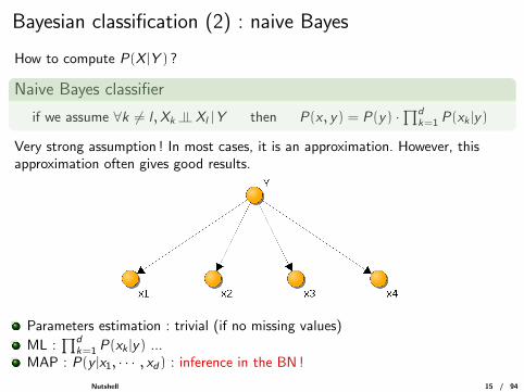
Bayesian classification (2) : naive Bayes
How to compute P(X |Y ) ?
Naive Bayes classifier
if we assume ∀k 6= l ,Xk |= Xl |Y then P(x , y) = P(y) ·∏d
k=1 P(xk |y)
Very strong assumption ! In most cases, it is an approximation. However, thisapproximation often gives good results.
Parameters estimation : trivial (if no missing values)
ML :∏d
k=1 P(xk |y) ...MAP : P(y |x1, · · · , xd) : inference in the BN !
Nutshell 15 / 94
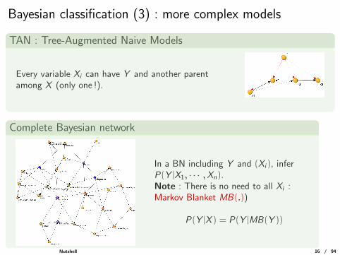
Bayesian classification (3) : more complex models
TAN : Tree-Augmented Naive Models
Every variable Xi can have Y and another parentamong X (only one !).
Complete Bayesian network
In a BN including Y and (Xi ), inferP(Y |X1, · · · ,Xn).Note : There is no need to all Xi :Markov Blanket MB(.))
P(Y |X ) = P(Y |MB(Y ))
Nutshell 16 / 94
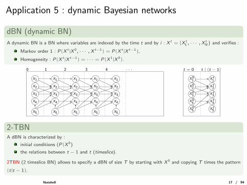
Application 5 : dynamic Bayesian networks
dBN (dynamic BN)
A dynamic BN is a BN where variables are indexed by the time t and by i : X t = {X t1 , · · · ,X
tN} and verifies :
Markov order 1 : P(X t |X 0, · · · ,X t−1) = P(X t |X t−1),
Homogeneity : P(X t |X t−1) = · · · = P(X 1|X 0).
X3
X4
X1
X2
X3
X4
X1
X2
X3
X4
X1
X2
X3
X4
X5 X5 X5 X5 X5
10 2 3 4 · · ·
X1
X2
X3
X4
X1
X2
t = 0 t | (t − 1)
X01
X02
X03
X04
X05
Xt1
Xt2
Xt3
Xt4
Xt5
2-TBNA dBN is characterized by :
initial conditions (P(X 0)
the relations between t − 1 and t (timeslice).
2TBN (2 timeslice BN) allows to specify a dBN of size T by starting with X 0 and copying T times the pattern
(t|t − 1).
Nutshell 17 / 94
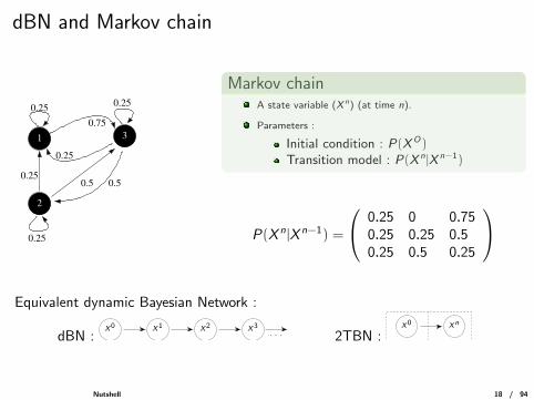
dBN and Markov chain
2
0.25
0.75
0.25
0.25
0.250.50.5
0.25
1 3
Markov chainA state variable (X n) (at time n).
Parameters :
Initial condition : P(XO)Transition model : P(X n |X n−1)
P(X n|X n−1) =
0.25 0 0.750.25 0.25 0.50.25 0.5 0.25
Equivalent dynamic Bayesian Network :
dBN : · · ·X3X2X1X0
2TBN :X0 Xn
Nutshell 18 / 94
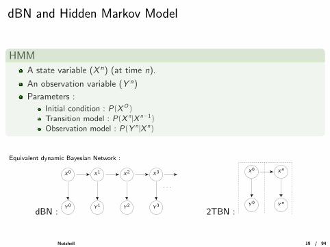
dBN and Hidden Markov Model
HMM
A state variable (X n) (at time n).
An observation variable (Y n)
Parameters :
Initial condition : P(XO)Transition model : P(X n |X n−1)Observation model : P(Y n |X n)
Equivalent dynamic Bayesian Network :
dBN :
X0
Y 0 Y 1 Y 2 Y 3
· · ·
X3X2X1
2TBN :Yn
X0 Xn
Y 0
Nutshell 19 / 94

Foundations
Nutshell 20 / 94
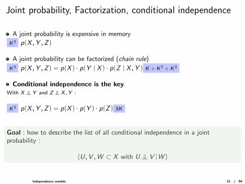
Joint probability, Factorization, conditional independence
A joint probability is expensive in memory
K3 p(X ,Y ,Z )
A joint probability can be factorized (chain rule)
K3 p(X ,Y ,Z ) = p(X ) · p(Y | X ) · p(Z | X ,Y ) K + K2 + K3
Conditional independence is the key.With X |= Y and Z |= X ,Y :
K3 p(X ,Y ,Z ) = p(X ) · p(Y ) · p(Z ) 3K
Goal : how to describe the list of all conditional independence in a jointprobability :
{U,V ,W ⊂ X with U |= V |W }
Independence models 21 / 94
Independence model
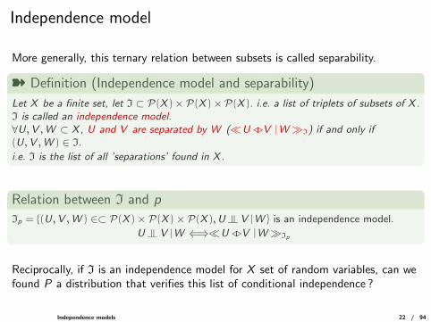
More generally, this ternary relation between subsets is called separability.
ý Definition (Independence model and separability)
Let X be a finite set, let I ⊂ P(X )×P(X )×P(X ). i.e. a list of triplets of subsets of X .I is called an independence model.∀U,V ,W ⊂ X , U and V are separated by W (�U /.V |W�I) if and only if(U,V ,W ) ∈ I.
i.e. I is the list of all ’separations’ found in X .
Relation between I and p
Ip = {(U,V ,W ) ∈⊂ P(X )× P(X )× P(X ),U |= V |W } is an independence model.
U |= V |W ⇐⇒�U /.V |W�Ip
Reciprocally, if I is an independence model for X set of random variables, can wefound P a distribution that verifies this list of conditional independence ?
Independence models 22 / 94
Semi-graphoid and graphoid
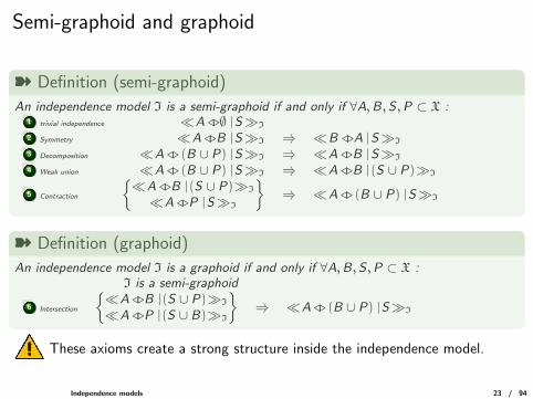
ý Definition (semi-graphoid)
An independence model I is a semi-graphoid if and only if ∀A,B,S ,P ⊂ X :1 trivial independence �A /.∅ |S�I
2 Symmetry �A /.B |S�I ⇒ �B /.A |S�I
3 Decomposition �A /. (B ∪ P) |S�I ⇒ �A /.B |S�I
4 Weak union �A /. (B ∪ P) |S�I ⇒ �A /.B |(S ∪ P)�I
5 Contraction
{�A /.B |(S ∪ P)�I
�A /.P |S�I
} ⇒ �A /. (B ∪ P) |S�I
ý Definition (graphoid)
An independence model I is a graphoid if and only if ∀A,B,S ,P ⊂ X :I is a semi-graphoid
6 Intersection
{�A /.B |(S ∪ P)�I
�A /.P |(S ∪ B)�I
} ⇒ �A /. (B ∪ P) |S�I
These axioms create a strong structure inside the independence model.
Independence models 23 / 94
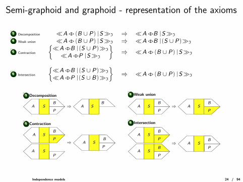
Semi-graphoid and graphoid - representation of the axioms
3 Decomposition �A /. (B ∪ P) |S�I ⇒ �A /.B |S�I
4 Weak union �A /. (B ∪ P) |S�I ⇒ �A /.B |(S ∪ P)�I
5 Contraction
{�A /.B |(S ∪ P)�I
�A /.P |S�I
} ⇒ �A /. (B ∪ P) |S�I
6 Intersection
{�A /.B |(S ∪ P)�I
�A /.P |(S ∪ B)�I
} ⇒ �A /. (B ∪ P) |S�I
6 Intersection
⇒ AB
SA SB
P
⇒ A SB
P
A SB
A SP
P
⇒A SB
PA S
B
P
⇒A S
B
P
B
PSA
A SB
P
5 Contraction
3 Decomposition 4 Weak union
Independence models 24 / 94
Semi-graphoid and graphoid
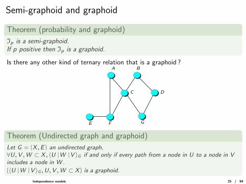
Theorem (probability and graphoid)
Ip is a semi-graphoid.If p positive then Ip is a graphoid.
Is there any other kind of ternary relation that is a graphoid ?
G
A B
C D
E F
Theorem (Undirected graph and graphoid)
Let G = (X ,E ) an undirected graph,∀U,V ,W ⊂ X , 〈U |W |V 〉G if and only if every path from a node in U to a node in Vincludes a node in W .
{〈U |W |V 〉G ,U,V ,W ⊂ X } is a graphoid.
Independence models 25 / 94
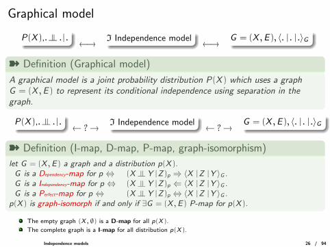
Graphical model
P(X ),. |= . | . ←→ I Independence model ←→ G = (X ,E ), 〈. | . | .〉G
ý Definition (Graphical model)
A graphical model is a joint probability distribution P(X ) which uses a graphG = (X ,E ) to represent its conditional independence using separation in thegraph.
P(X ),. |= . | . ← ?→ I Independence model ← ?→ G = (X ,E ), 〈. | . | .〉G
ý Definition (I-map, D-map, P-map, graph-isomorphism)
let G = (X ,E ) a graph and a distribution p(X ).G is a Dependency-map for p ⇔ (X |= Y |Z )p ⇒ 〈X |Z |Y 〉G .G is a Independency-map for p ⇔ (X |= Y |Z )p ⇐ 〈X |Z |Y 〉G .G is a Perfect-map for p ⇔ (X |= Y |Z )p ⇔ 〈X |Z |Y 〉G .
p(X ) is graph-isomorph if and only if ∃G = (X ,E ) P-map for p(X ).
The empty graph (X , ∅) is a D-map for all p(X).
The complete graph is a I-map for all distribution p(X).
Independence models 26 / 94
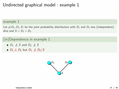
Undirected graphical model : example 1
example 1
Let p(D1,D2,S) be the joint probability distribution with D1 and D2 two (independent)
dice and S = D1 + D2.
(in)Dependence in example 1
D1 6 |= S and D2 6 |= SD1 |= D2 but D1 6 |= D2 |S
D1 D2
S
Independence models 27 / 94
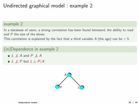
Undirected graphical model : example 2
example 2In a database of users, a strong correlation has been found betweenL the ability to readand P the size of the shoes.
This correlation is explained by the fact that a third variable A (the age) can be < 5.
(in)Dependence in example 2
L 6 |= A and P 6 |= AL 6 |= P but L |= P |A
L
A
P
Independence models 28 / 94
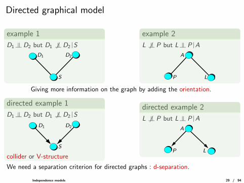
Directed graphical model
example 1
D1 |= D2 but D1 6 |= D2 |S
D1 D2
S
example 2
L 6 |= P but L |= P |A
L
A
P
Giving more information on the graph by adding the orientation.
directed example 1
D1 |= D2 but D1 6 |= D2 |S
D1
S
D2
collider or V-structure
directed example 2
L 6 |= P but L |= P |A
A
P L
We need a separation criterion for directed graphs : d-separation.
Independence models 29 / 94
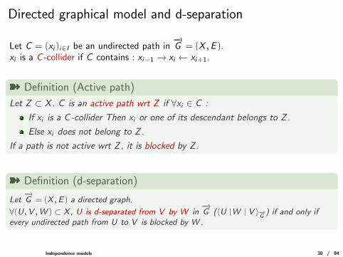
Directed graphical model and d-separation
Let C = (xi )i∈I be an undirected path in−→G = (X ,E ).
xi is a C -collider if C contains : xi−1 → xi ← xi+1.
ý Definition (Active path)
Let Z ⊂ X . C is an active path wrt Z if ∀xi ∈ C :
If xi is a C -collider Then xi or one of its descendant belongs to Z .
Else xi does not belong to Z .
If a path is not active wrt Z , it is blocked by Z .
ý Definition (d-separation)
Let−→G = (X ,E ) a directed graph,
∀(U,V ,W ) ⊂ X , U is d-separated from V by W in−→G (〈U |W | V 〉−→
G) if and only if
every undirected path from U to V is blocked by W .
Independence models 30 / 94
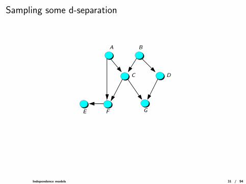
Sampling some d-separation
G
A B
C D
E F
Independence models 31 / 94
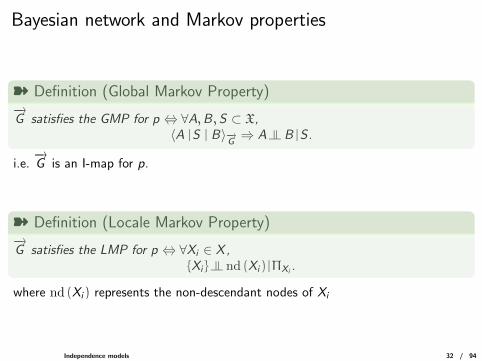
Bayesian network and Markov properties
ý Definition (Global Markov Property)−→G satisfies the GMP for p ⇔ ∀A,B, S ⊂ X,
〈A |S | B〉−→G⇒ A |= B |S .
i.e.−→G is an I-map for p.
ý Definition (Locale Markov Property)−→G satisfies the LMP for p ⇔ ∀Xi ∈ X ,
{Xi } |= nd (Xi ) |ΠXi .
where nd (Xi ) represents the non-descendant nodes of Xi
Independence models 32 / 94
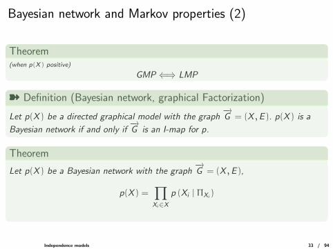
Bayesian network and Markov properties (2)
Theorem(when p(X) positive)
GMP ⇐⇒ LMP
ý Definition (Bayesian network, graphical Factorization)
Let p(X ) be a directed graphical model with the graph−→G = (X ,E ). p(X ) is a
Bayesian network if and only if−→G is an I-map for p.
Theorem
Let p(X ) be a Bayesian network with the graph−→G = (X ,E ),
p(X ) =∏Xi∈X
p (Xi | ΠXi )
Independence models 33 / 94
Markov Equivalence class
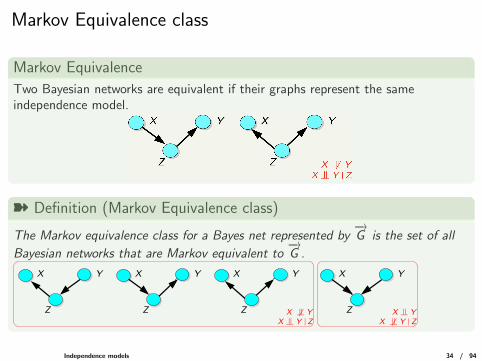
Markov Equivalence
Two Bayesian networks are equivalent if their graphs represent the sameindependence model.
ý Definition (Markov Equivalence class)
The Markov equivalence class for a Bayes net represented by−→G is the set of all
Bayesian networks that are Markov equivalent to−→G .
XX Y
Z
Y
Z
X Y
Z
X Y
Z X |= YX 6 |= Y |Z
X 6 |= YX |= Y |Z
Independence models 34 / 94
Causality
Independence models 35 / 94
Causality and probability
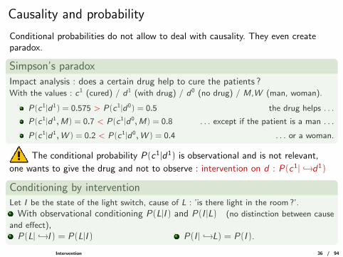
Conditional probabilities do not allow to deal with causality. They even createparadox.
Simpson’s paradox
Impact analysis : does a certain drug help to cure the patients ?With the values : c1 (cured) / d1 (with drug) / d0 (no drug) / M,W (man, woman).
P(c1|d1) = 0.575 > P(c1|d0) = 0.5 the drug helps . . .
P(c1|d1,M) = 0.7 < P(c1|d0,M) = 0.8 . . . except if the patient is a man . . .
P(c1|d1,W ) = 0.2 < P(c1|d0,W ) = 0.4 . . . or a woman.
The conditional probability P(c1|d1) is observational and is not relevant,
one wants to give the drug and not to observe : intervention on d : P(c1| ↪→d1)
Conditioning by interventionLet I be the state of the light switch, cause of L : ’is there light in the room ?’.
With observational conditioning P(L|I ) and P(I |L) (no distinction between cause
and effect),P(L| ↪→I ) = P(L|I ) P(I | ↪→L) = P(I ).
Intervention 36 / 94
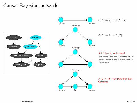
Causal Bayesian network
CancerSmoke
P(C |↪→S) = P(C | S)
Smoke
Genotype
Cancer
P(C |↪→S) = P(C)
Smoke
Genotype
Cancer
P(C |↪→S) unknown !We do not know how to differentiate the
causal impact of the 2 causes from the
observation.
CancerSmoke
Genotype
Tar
P(C |↪→S) computable ! Do-Calculus
Intervention 37 / 94
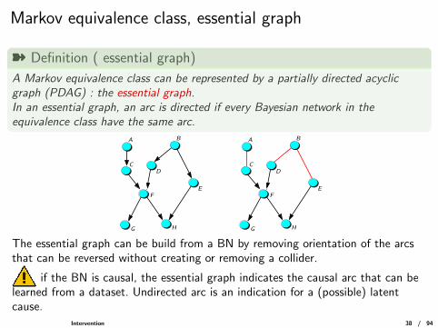
Markov equivalence class, essential graph
ý Definition ( essential graph)
A Markov equivalence class can be represented by a partially directed acyclicgraph (PDAG) : the essential graph.In an essential graph, an arc is directed if every Bayesian network in theequivalence class have the same arc.
HH
A B
CD
EF
G
A B
CD
EF
G
The essential graph can be build from a BN by removing orientation of the arcsthat can be reversed without creating or removing a collider.
if the BN is causal, the essential graph indicates the causal arc that can belearned from a dataset. Undirected arc is an indication for a (possible) latentcause.
Intervention 38 / 94
Learning
Intervention 39 / 94
What can we learn ?
Learning in Bayesian network
The goal of a learning algorithm is to estimate from a dataset and from prior :
the structure of the Bayesian network (is X parent of Y ?)
the parameters of the Bayesian network (P(X = 0 | Y = 1) ?)The dataset can be :
complete,
incomplete (missing values).
The prior knowledge can be for instance :
(part of) the structure of the BN,
The probability distribution for certain variables, etc.
Therefore 4 main classes of learning algorithms in BN :“Learning of {parameters |structure} with {complete |incomplete} data”.
Learning 40 / 94
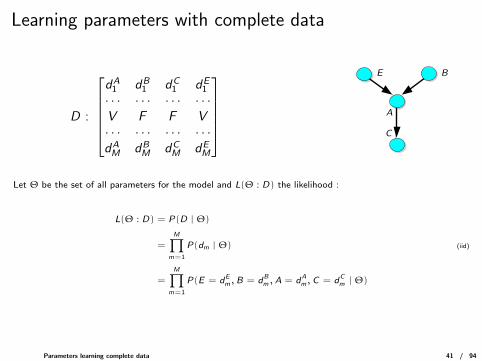
Learning parameters with complete data
D :
dA
1 dB1 dC
1 dE1
· · · · · · · · · · · ·V F F V· · · · · · · · · · · ·dAM dB
M dCM dE
M
C
E B
A
Let Θ be the set of all parameters for the model and L(Θ : D) the likelihood :
L(Θ : D) = P(D | Θ)
=
M∏m=1
P(dm | Θ) (iid)
=
M∏m=1
P(E = dEm,B = dB
m ,A = dAm,C = dC
m | Θ)
Parameters learning complete data 41 / 94
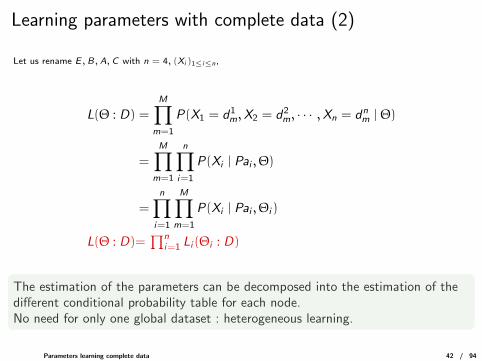
Learning parameters with complete data (2)
Let us rename E ,B,A,C with n = 4, (Xi)1≤i≤n,
L(Θ : D) =
M∏m=1
P(X1 = d1m,X2 = d2
m, · · · ,Xn = dnm | Θ)
=
M∏m=1
n∏i=1
P(Xi | Pai , Θ)
=
n∏i=1
M∏m=1
P(Xi | Pai , Θi )
L(Θ : D)=∏n
i=1 Li (Θi : D)
The estimation of the parameters can be decomposed into the estimation of thedifferent conditional probability table for each node.No need for only one global dataset : heterogeneous learning.
Parameters learning complete data 42 / 94
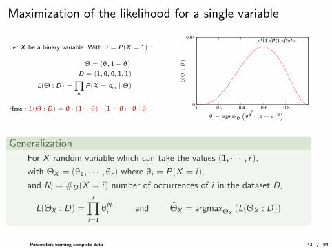
Maximization of the likelihood for a single variable
Let X be a binary variable. With θ = P(X = 1) :
Θ = {θ, 1 − θ}
D = (1, 0, 0, 1, 1)
L(Θ : D) =∏m
P(X = dm | Θ)
Here : L(Θ : D) = θ · (1 − θ) · (1 − θ) · θ · θ.
x*(1-x)*(1-x)*x*x0.04
0 0.2 0.4 0.6 0.8 1
L(Θ
:D)
θ
0
θ = argmaxθ
(θ3 · (1 − θ)2
)
Generalization
For X random variable which can take the values (1, · · · , r),with ΘX = (θ1, · · · , θr ) where θi = P(X = i),
and Ni = #D(X = i) number of occurrences of i in the dataset D,
L(ΘX : D) =
r∏i=1
θNi
i and ΘX = argmaxΘX(L(ΘX : D))
Parameters learning complete data 43 / 94
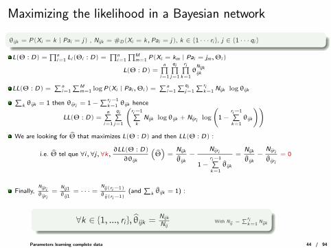
Maximizing the likelihood in a Bayesian network
θijk = P(Xi = k | Pai = j) , Nijk = #D(Xi = k,Pai = j), k ∈ {1 · · · ri }, j ∈ {1 · · · qi }
L(Θ : D) =∏n
i=1 Li(Θi : D) =∏n
i=1
∏Mm=1 P(Xi = km | Pai = jm, Θi)
L(Θ : D) =n∏
i=1
qi∏j=1
ri∏k=1
θNijkijk
LL(Θ : D) =∑n
i=1
∑Mm=1 log P(Xi | Pai , Θi) =
∑ni=1
∑qij=1
∑rik=1 Nijk log θijk∑
k θijk = 1 then θijri= 1 −
∑ri−1
k=1 θijk hence
LL(Θ : D) =n∑
i=1
qi∑j=1
(ri−1∑k
Nijk log θijk + Nijrilog
(1 −
ri−1∑k=1
θijk
))
We are looking for Θ that maximizes L(Θ : D) and then LL(Θ : D) :
i.e. Θ tel que ∀i, ∀j, ∀k,∂LL(Θ : D)
∂θijk
(Θ)
=Nijk
θijk
−Nijri
1 −ri−1∑k=1
θijk
=Nijk
θijk
−Nijri
θijri
= 0
Finally,Nijriθijri
=Nij1
θij1= · · · =
Nij(ri−1)
θij(ri−1)(and
∑k θijk = 1) :
∀k ∈ {1, ..., ri }, θijk =Nijk
NijWith Nij =
∑rik=1
Nijk
Parameters learning complete data 44 / 94
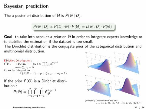
Bayesian prediction
The a posteriori distribution of Θ is P(Θ | D).
P(Θ | D) ∝ P(D | Θ) ·P(Θ) = L(Θ : D) ·P(Θ)
Goal to take into account a prior on Θ in order to integrate experts knowledge orto stabilize the estimation if the dataset is too small.The Dirichlet distribution is the conjugate prior of the categorical distribution andmultinomial distribution.
Dirichlet Distribution :f (p1, · · · , pK ;α1, · · ·αK ) ∝
∏Ki=1 x
αi−1
i(where
∑i pi = 1)
f can be interpret as :P (P(X = i) = pi | #X=i = αi − 1)
If the prior P(Θ) is a Dirichlet distri-bution :
P(Θ) =n∏
i=1
qi∏j=1
ri∏k=1
θαijk−1ijk
[Wikipedia] Clockwise from top left :α = (6, 2, 2), (3, 7, 5), (6, 2, 6), (2, 3, 4).
Parameters learning complete data 45 / 94
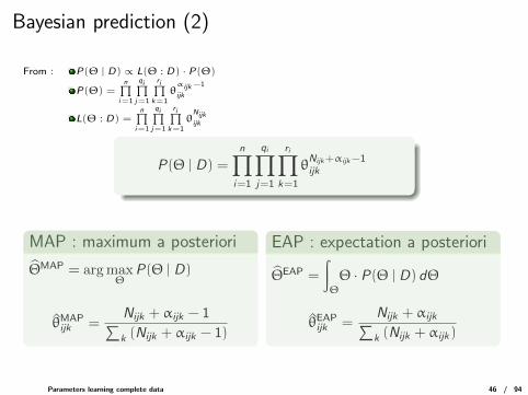
Bayesian prediction (2)
From : P(Θ | D) ∝ L(Θ : D) · P(Θ)
P(Θ) =n∏
i=1
qi∏j=1
ri∏k=1
θαijk−1
ijk
L(Θ : D) =n∏
i=1
qi∏j=1
ri∏k=1
θNijkijk
P(Θ | D) =
n∏i=1
qi∏j=1
ri∏k=1
θNijk+αijk−1ijk
MAP : maximum a posteriori
ΘMAP = argmaxΘ
P(Θ | D)
θMAPijk =
Nijk + αijk − 1∑k (Nijk + αijk − 1)
EAP : expectation a posteriori
ΘEAP =
∫Θ
Θ · P(Θ | D) dΘ
θEAPijk =
Nijk + αijk∑k (Nijk + αijk)
Parameters learning complete data 46 / 94
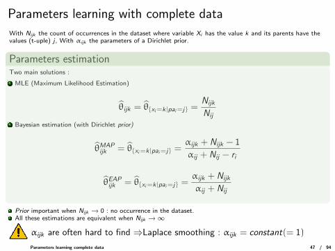
Parameters learning with complete data
With Nijk the count of occurrences in the dataset where variable Xi has the value k and its parents have thevalues (t-uple) j , With αijk the parameters of a Dirichlet prior.
Parameters estimationTwo main solutions :
MLE (Maximum Likelihood Estimation)
θijk = θ{xi=k|pai=j} =Nijk
Nij
Bayesian estimation (with Dirichlet prior)
θMAPijk = θ{xi=k|pai=j} =
αijk + Nijk − 1
αij + Nij − ri
θEAPijk = θ{xi=k|pai=j} =αijk + Nijk
αij + Nij
Prior important when Nijk → 0 : no occurrence in the dataset.All these estimations are equivalent when Nijk → ∞
αijk are often hard to find ⇒Laplace smoothing : αijk = constant(= 1)
Parameters learning complete data 47 / 94
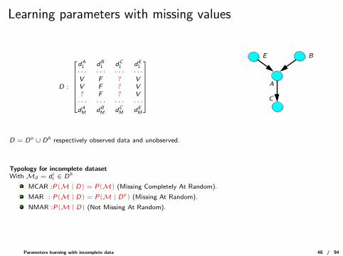
Learning parameters with missing values
D :
dA1 dB
1 dC1 dE
1· · · · · · · · · · · ·V F ? VV F ? V? F ? V· · · · · · · · · · · ·dAM dB
M dCM dE
M
C
E B
A
D = Do ∪ Dh respectively observed data and unobserved.
Typology for incomplete datasetWith Mil = d i
l ∈ Dh
MCAR :P(M | D) = P(M) (Missing Completely At Random).
MAR : P(M | D) = P(M | Do) (Missing At Random).
NMAR :P(M | D) (Not Missing At Random).
Parameters learning with incomplete data 48 / 94
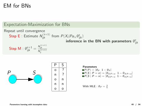
EM for BNs
Expectation-Maximization for BNs
Repeat until convergence
Step E : Estimate N(t+1)ijk from P(Xi |Pai , θ
tijk)
inference in the BN with parameters θtijk
Step M : θt+1ijk =
N(t+1)ijk
N(t+1)ij
P S
P So ?n ?o nn no o
ParametersP(P) = [θP 1 − θP ]P(S | P = o) = [θS|P=o 1 − θS|P=o ]P(S | P = n) = [θS|P=n 1 − θS|P=n]
With MLE : θP = 35
Parameters learning with incomplete data 49 / 94
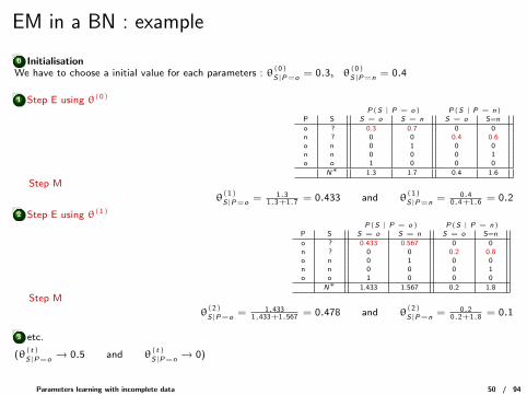
EM in a BN : example
0 InitialisationWe have to choose a initial value for each parameters : θ
(0)
S|P=o= 0.3, θ
(0)
S|P=n= 0.4
1 Step E using θ(0)
P(S | P = o) P(S | P = n)P S S = o S = n S = o S=n
o ? 0.3 0.7 0 0n ? 0 0 0.4 0.6o n 0 1 0 0n n 0 0 0 1o o 1 0 0 0
N∗ 1.3 1.7 0.4 1.6
Step M
θ(1)
S|P=o= 1.3
1.3+1.7 = 0.433 and θ(1)
S|P=n= 0.4
0.4+1.6 = 0.2
2 Step E using θ(1)
P(S | P = o) P(S | P = n)P S S = o S = n S = o S=n
o ? 0.433 0.567 0 0n ? 0 0 0.2 0.8o n 0 1 0 0n n 0 0 0 1o o 1 0 0 0
N∗ 1.433 1.567 0.2 1.8
Step M
θ(2)
S|P=o= 1.433
1.433+1.567 = 0.478 and θ(2)
S|P=n= 0.2
0.2+1.8 = 0.1
3 etc.
(θ(t)
S|P=o→ 0.5 and θ
(t)
S|P=n→ 0)
Parameters learning with incomplete data 50 / 94
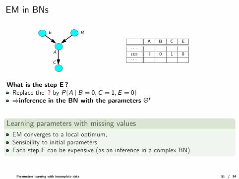
EM in BNs
C
E B
A
A B C E
· · ·1325 ? 0 1 0· · ·
What is the step E ?Replace the ? by P(A | B = 0,C = 1,E = 0)⇒inference in the BN with the parameters Θt
Learning parameters with missing values
EM converges to a local optimum,Sensibility to initial parametersEach step E can be expensive (as an inference in a complex BN)
Parameters learning with incomplete data 51 / 94
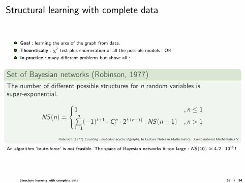
Structural learning with complete data
Goal : learning the arcs of the graph from data.
Theoretically : χ2 test plus enumeration of all the possible models : OK
In practice : many different problems but above all :
Set of Bayesian networks (Robinson, 1977)
The number of different possible structures for n random variables issuper-exponential.
NS(n) =
1 , n ≤ 1n∑
i=1
(−1)i+1 · C ni · 2i·(n−i) · NS(n − 1) , n > 1
Robinson (1977) Counting unlabelled acyclic digraphs. In Lecture Notes in Mathematics : Combinatorial Mathematics V
An algorithm ’brute-force’ is not feasible. The space of Bayesian networks it too large : NS(10) ≈ 4.2 · 1018 !
Structure learning with complete data 52 / 94
Structural learning - introduction
General picture of structural learning
Identification of symmetrical relation (independence) + orientation
algorithm IC/PCalgorithm IC*/FCI
Important for causal models.
Local search
In the (very large) space of structures,Greedy algorithms maximizing a score (entropy, AIC, BIC, MDL,BD, BDe,BDeu, · · · ).
Structure learning with complete data 53 / 94
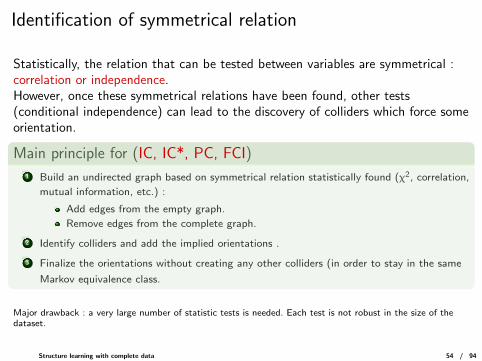
Identification of symmetrical relation
Statistically, the relation that can be tested between variables are symmetrical :correlation or independence.However, once these symmetrical relations have been found, other tests(conditional independence) can lead to the discovery of colliders which force someorientation.
Main principle for (IC, IC*, PC, FCI)
1 Build an undirected graph based on symmetrical relation statistically found (χ2, correlation,
mutual information, etc.) :
Add edges from the empty graph.
Remove edges from the complete graph.
2 Identify colliders and add the implied orientations .
3 Finalize the orientations without creating any other colliders (in order to stay in the same
Markov equivalence class.
Major drawback : a very large number of statistic tests is needed. Each test is not robust in the size of thedataset.
Structure learning with complete data 54 / 94
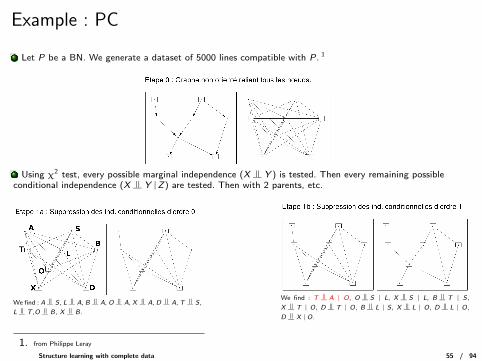
Example : PC
Let P be a BN. We generate a dataset of 5000 lines compatible with P. 1
Using χ2 test, every possible marginal independence (X |= Y ) is tested. Then every remaining possibleconditional independence (X |= Y |Z) are tested. Then with 2 parents, etc.
We find : A |= S , L |= A, B |= A, O |= A, X |= A, D |= A, T |= S ,
L |= T ,O |= B, X |= B.
We find : T |= A | O, O |= S | L, X |= S | L, B |= T | S ,
X |= T | O, D |= T | O, B |= L | S, X |= L | O, D |= L | O,
D |= X |O.
1. from Philippe Leray
Structure learning with complete data 55 / 94
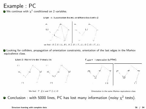
Example : PCWe continue with χ2 conditioned on 2 variables.
we find : D |= S |(L, B), X |= O |(T, L), D |= O |(T, L).
Looking for colliders, propagation of orientation constraints, orientation of the last edges in the Markovequivalence class.
We find : T 6 |= L and T |= L |O Orientation in the same Markov equivalence class.
Conclusion : with 5000 lines, PC has lost many information (noisy χ2 tests).
Structure learning with complete data 56 / 94
Structural learning with local search
Local searchA local search is composed of :
a space of all possible solutions (search space),
a neighborhood defined by elementary transformations of a solution.Theneighbors of a solution are the solutions that can be obtained by theapplication of an elementary transformation.
a score (heurisitic) that evaluates the quality of a solution.
From an initial solution, the local search then produces a sequence of solutionssuch that every solution in the sequence has a better score than the precedentsolutions in the sequence (Greedy Search).
Local search in Bayesian networks
space of Bayesian networks (huge)
The score (see next slide)
The initial solution (empty Bayesian network for instance)
Elementary operations : add/remove/reverse an arc
Structure learning with complete data 57 / 94
Scores
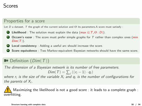
Properties for a scoreLet D a dataset, T the graph of the current solution and Θ its parameters.A score must satissfy :
1 Likelihood : The solution must explain the data (max L(T , Θ : D)).
2 Occam’s razor : The score must prefer simple graphs for T rather than complex ones (minDim(T )).
3 Local consistency : Adding a useful arc should increase the score.
4 Score equivalence : Two Markov-equivalent Bayesian networks should have the same score.
ý Definition (Dim(T ))
The dimension of a Bayesian network is its number of free parameters.Dim(T ) =
∑i ((ri − 1) · qi )
where ri is the size of the variable Xi and qi is the number of configurations forthe parents of Xi .
Maximizing the likelihood is not a good score : it leads to a complete graph :overfitting.
Structure learning with complete data 58 / 94
Some scores (1) : AIC/BIC
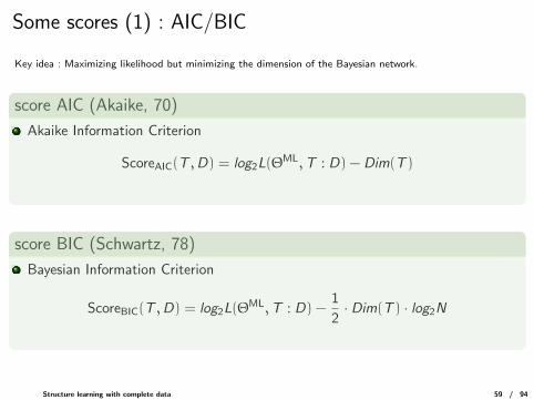
Key idea : Maximizing likelihood but minimizing the dimension of the Bayesian network.
score AIC (Akaike, 70)
Akaike Information Criterion
ScoreAIC(T ,D) = log2L(ΘML,T : D) − Dim(T )
score BIC (Schwartz, 78)
Bayesian Information Criterion
ScoreBIC(T ,D) = log2L(ΘML,T : D) −
1
2· Dim(T ) · log2N
Structure learning with complete data 59 / 94
Minimum Description Length (Rissanen,78)
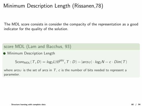
The MDL score consists in consider the compacity of the representation as a goodindicator for the quality of the solution.
score MDL (Lam and Bacchus, 93)
Minimum Description Length
ScoreMDL(T ,D) = log2L(ΘMV,T : D) − |arcsT | · log2N − c · Dim(T )
where arcsT is the set of arcs in T , c is the number of bits needed to represent aparameter.
Structure learning with complete data 60 / 94
Bayesian Dirichlet score Equivalent
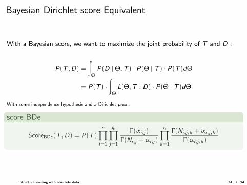
With a Bayesian score, we want to maximize the joint probability of T and D :
P(T ,D) =
∫Θ
P(D | Θ,T ) · P(Θ | T ) · P(T )dΘ
= P(T ) ·∫Θ
L(Θ,T : D) · P(Θ | T )dΘ
With some independence hypothesis and a Dirichlet prior :
score BDe
ScoreBDe(T ,D) = P(T )
n∏i=1
qi∏j=1
Γ(αi,j)
Γ(Ni,j + αi,j)
ri∏k=1
Γ(Ni,j,k + αi,j,k)
Γ(αi,j,k)
Structure learning with complete data 61 / 94
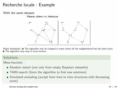
Recherche locale : Example
With the same dataset.
Major drawbacks : The algorithm may be trapped in zones where all the neighborhood has the same score.The algorithm may stop in local minima.
SolutionsMeta-heuristic :
Random restart (not only from empty Bayesian networks)
TABU-search (force the algorithm to find new solutions)
Simulated annealing (accept from time to time structures with decreasingscore)
Structure learning with complete data 62 / 94
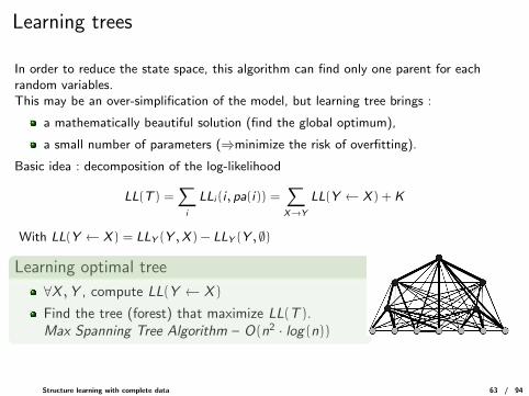
Learning trees
In order to reduce the state space, this algorithm can find only one parent for eachrandom variables.This may be an over-simplification of the model, but learning tree brings :
a mathematically beautiful solution (find the global optimum),
a small number of parameters (⇒minimize the risk of overfitting).
Basic idea : decomposition of the log-likelihood
LL(T ) =∑i
LLi (i , pa(i)) =∑X→Y
LL(Y ← X ) + K
With LL(Y ← X ) = LLY (Y ,X ) − LLY (Y , ∅)
Learning optimal tree
∀X ,Y , compute LL(Y ← X )
Find the tree (forest) that maximize LL(T ).Max Spanning Tree Algorithm – O(n2 · log(n))
Structure learning with complete data 63 / 94
Inference
Structure learning with complete data 64 / 94
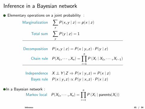
Inference in a Bayesian network
Elementary operations on a joint probability :
Marginalization∑y
P(x , y | z) = p(x | z)
Total sum∑y
P(y | z) = 1
Decomposition P(x , y | z) = P(x | y , z) · P(y | z)
Chain rule P(X1, · · · ,Xn) =
n∏i=1
P (Xi | X1, · · · ,Xi−1)
Independence X |= Y |Z ⇒ P(x | y , z) = P(x | z)
Bayes rule P(x | y , z) ∝ P(y | x , z) · P(x | z)
In a Bayesian network :
Markov local P(X1, · · · ,Xn) =
n∏i=1
P (Xi | parents(Xi ))
Inference 65 / 94
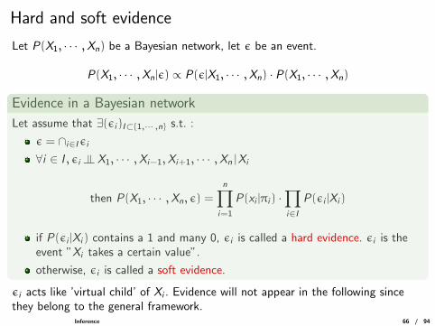
Hard and soft evidence
Let P(X1, · · · ,Xn) be a Bayesian network, let ε be an event.
P(X1, · · · ,Xn|ε) ∝ P(ε|X1, · · · ,Xn) · P(X1, · · · ,Xn)
Evidence in a Bayesian network
Let assume that ∃(εi )I⊂{1,··· ,n} s.t. :
ε = ∩i∈Iεi∀i ∈ I , εi |= X1, · · · ,Xi−1,Xi+1, · · · ,Xn |Xi
then P(X1, · · · ,Xn, ε) =
n∏i=1
P(xi |πi ) ·∏i∈I
P(εi |Xi )
if P(εi |Xi ) contains a 1 and many 0, εi is called a hard evidence. εi is theevent ”Xi takes a certain value”.
otherwise, εi is called a soft evidence.
εi acts like ’virtual child’ of Xi . Evidence will not appear in the following sincethey belong to the general framework.
Inference 66 / 94
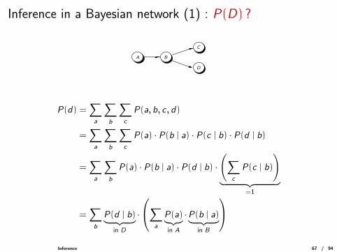
Inference in a Bayesian network (1) : P(D) ?
A B
C
D
P(d) =∑a
∑b
∑c
P(a, b, c , d)
=∑a
∑b
∑c
P(a) · P(b | a) · P(c | b) · P(d | b)
=∑a
∑b
P(a) · P(b | a) · P(d | b) ·
(∑c
P(c | b)
)︸ ︷︷ ︸
=1
=∑b
P(d | b)︸ ︷︷ ︸in D
·
∑a
P(a)︸︷︷︸in A
·P(b | a)︸ ︷︷ ︸in B
Inference 67 / 94
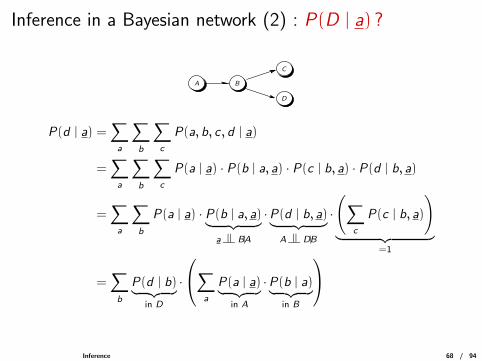
Inference in a Bayesian network (2) : P(D | a) ?
A B
C
D
P(d | a) =∑a
∑b
∑c
P(a, b, c , d | a)
=∑a
∑b
∑c
P(a | a) · P(b | a, a) · P(c | b, a) · P(d | b, a)
=∑a
∑b
P(a | a) · P(b | a, a)︸ ︷︷ ︸a |= B|A
·P(d | b, a)︸ ︷︷ ︸A |= D|B
·
(∑c
P(c | b, a)
)︸ ︷︷ ︸
=1
=∑b
P(d | b)︸ ︷︷ ︸in D
·
∑a
P(a | a)︸ ︷︷ ︸in A
·P(b | a)︸ ︷︷ ︸in B
Inference 68 / 94
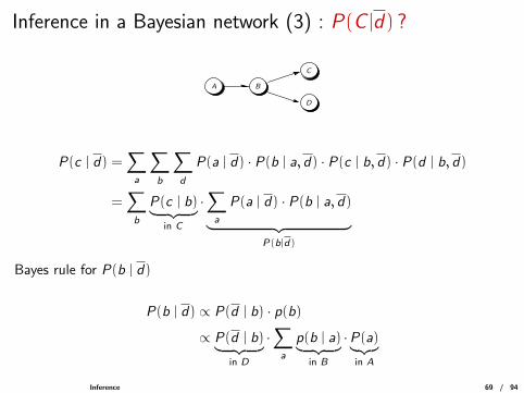
Inference in a Bayesian network (3) : P(C |d) ?
A B
C
D
P(c | d) =∑a
∑b
∑d
P(a | d) · P(b | a, d) · P(c | b, d) · P(d | b, d)
=∑b
P(c | b)︸ ︷︷ ︸in C
·∑a
P(a | d) · P(b | a, d)︸ ︷︷ ︸P(b|d)
Bayes rule for P(b | d)
P(b | d) ∝ P(d | b) · p(b)
∝ P(d | b)︸ ︷︷ ︸in D
·∑a
p(b | a)︸ ︷︷ ︸in B
·P(a)︸︷︷︸in A
Inference 69 / 94
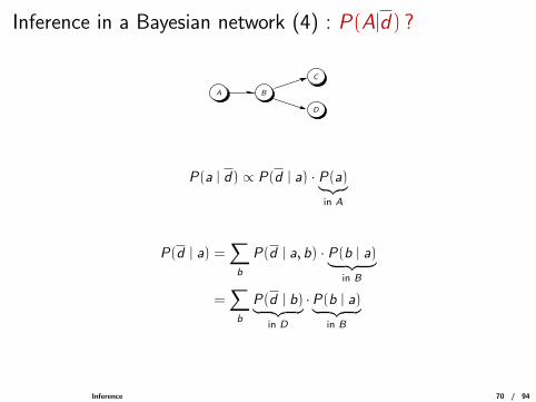
Inference in a Bayesian network (4) : P(A|d) ?
A B
C
D
P(a | d) ∝ P(d | a) · P(a)︸︷︷︸in A
P(d | a) =∑b
P(d | a, b) · P(b | a)︸ ︷︷ ︸in B
=∑b
P(d | b)︸ ︷︷ ︸in D
·P(b | a)︸ ︷︷ ︸in B
Inference 70 / 94
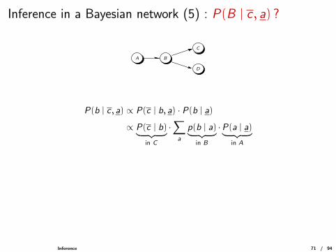
Inference in a Bayesian network (5) : P(B | c , a) ?
A B
C
D
P(b | c , a) ∝ P(c | b, a) · P(b | a)
∝ P(c | b)︸ ︷︷ ︸in C
·∑a
p(b | a)︸ ︷︷ ︸in B
·P(a | a)︸ ︷︷ ︸in A
Inference 71 / 94
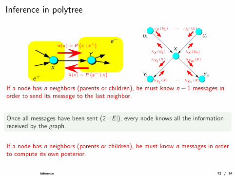
Inference in polytree
X
Y
π(x) = P(x | e+
)
e+
e−
λ(x) = P(e− | x
)
X
· · · πX (Un)
λX (Un)
πYm(X)
· · · λYm(X)
U1
Ym
Un
Y1
λY1(X)
πY1(X)
λX (U1)
πX (U1)
If a node has n neighbors (parents or children), he must know n − 1 messages inorder to send its message to the last neighbor.
Once all messages have been sent (2 · |E |), every node knows all the informationreceived by the graph.
If a node has n neighbors (parents or children), he must know n messages in orderto compute its own posterior.
Inference 72 / 94
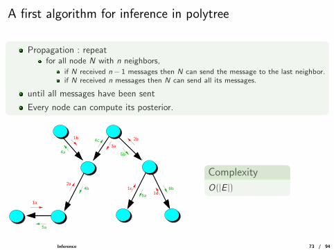
A first algorithm for inference in polytree
Propagation : repeatfor all node N with n neighbors,
if N received n − 1 messages then N can send the message to the last neighbor.if N received n messages then N can send all its messages.
until all messages have been sent
Every node can compute its posterior.
1a
1b
1c1d
2a
2b
3a
4a
4b
4c
5a
5b
6a
6b
Complexity
O(|E |)
Inference 73 / 94
Inference in polytree (2)
1a
1b
2a
2b3a
4a
4b
5a
6a6b
4c
5b
1d1c
1a
1b
2a
2b4a
5c
5d5a
5b1d
1c
3a
4b
6a
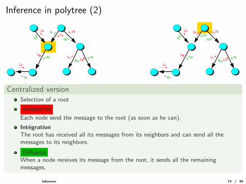
Centralized versionSelection of a root
Absorption
Each node send the message to the root (as soon as he can).
IntegrationThe root has received all its messages from its neighbors and can send all themessages to its neighbors.
DiffusionWhen a node receives its message from the root, it sends all the remainingmessages.
Inference 74 / 94
Problem with message passing algorithms in DAG
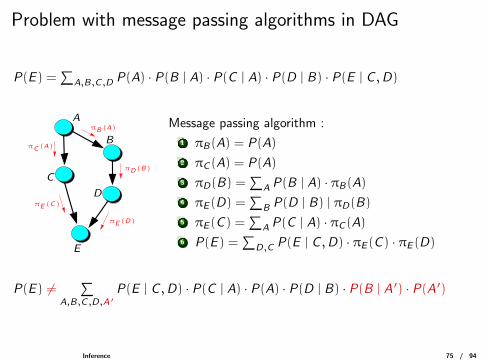
P(E ) =∑
A,B,C ,D P(A) · P(B | A) · P(C | A) · P(D | B) · P(E | C ,D)
D
B
A
E
C
πE (D)
πC (A)
πE (C)
πB(A)
πD(B)
Message passing algorithm :
1 πB(A) = P(A)
2 πC (A) = P(A)
3 πD(B) =∑
A P(B | A) · πB(A)4 πE (D) =
∑B P(D | B) | πD(B)
5 πE (C ) =∑
A P(C | A) · πC (A)6 P(E ) =
∑D,C P(E | C ,D) · πE (C ) · πE (D)
P(E ) 6=∑
A,B,C ,D,A ′P(E | C ,D) · P(C | A) · P(A) · P(D | B) · P(B | A ′) · P(A ′)
Inference 75 / 94
Inference in DAG
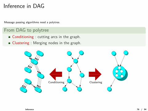
Message passing algorithms need a polytree.
From DAG to polytree
Conditioning : cutting arcs in the graph.
Clustering : Merging nodes in the graph.
ClusteringConditioning
Inference 76 / 94
Conditioning
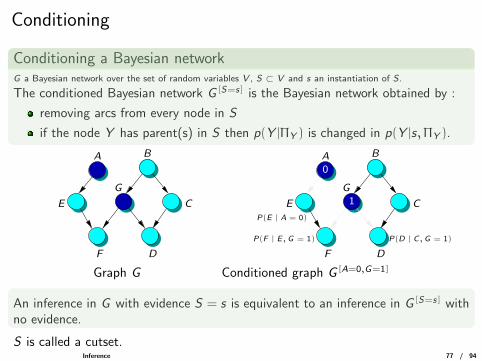
Conditioning a Bayesian networkG a Bayesian network over the set of random variables V , S ⊂ V and s an instantiation of S.
The conditioned Bayesian network G [S=s] is the Bayesian network obtained by :
removing arcs from every node in S
if the node Y has parent(s) in S then p(Y |ΠY ) is changed in p(Y |s, ΠY ).
A
F D
B
E C
G
A0
P(E | A = 0)
P(F | E , G = 1) P(D | C , G = 1)
F D
B
E C
G1
Graph G Conditioned graph G [A=0,G=1]
An inference in G with evidence S = s is equivalent to an inference in G [S=s] withno evidence.
S is called a cutset.Inference 77 / 94
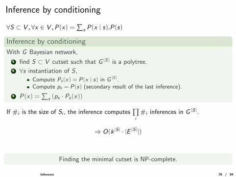
Inference by conditioning
∀S ⊂ V , ∀x ∈ V ,P(x) =∑
s P(x | s).P(s)
Inference by conditioning
With G Bayesian network,
1 find S ⊂ V cutset such that G [S] is a polytree.2 ∀s instantiation of S ,
Compute Ps(x) = P(x | s) in G [S].Compute ps = P(s) (secondary result of the last inference).
3 P(x) =∑
s (ps · Ps(x))
If #i is the size of Si , the inference computes∏i
#i inferences in G [S].
⇒ O(k |S| · |E [S]|)
Finding the minimal cutset is NP-complete.
Inference 78 / 94
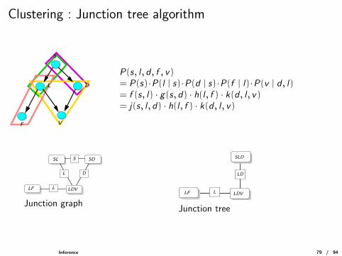
Clustering : Junction tree algorithm
L
F
S
D
V
P(s, l , d , f , v)= P(s)·P(l | s)·P(d | s)·P(f | l)·P(v | d , l)= f (s, l) · g(s, d) · h(l , f ) · k(d , l , v)= j(s, l , d) · h(l , f ) · k(d , l , v)
L
L
S
D
SL SD
LDVLF
Junction graph
L
LD
SLD
LDVLF
Junction tree
Inference 79 / 94
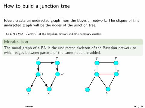
How to build a junction tree
Idea : create an undirected graph from the Bayesian network. The cliques of thisundirected graph will be the nodes of the junction tree.
The CPTs P(X | ParentX ) of the Bayesian network indicate necessary clusters.
MoralizationThe moral graph of a BN is the undirected skeleton of the Bayesian network towhich edges between parents of the same node are added.
V
S T
L
F
DL
S T
F V
D
Inference 80 / 94
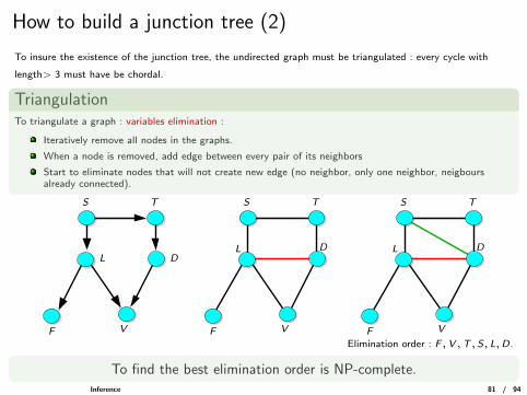
How to build a junction tree (2)
To insure the existence of the junction tree, the undirected graph must be triangulated : every cycle with
length> 3 must have be chordal.
TriangulationTo triangulate a graph : variables elimination :
Iteratively remove all nodes in the graphs.
When a node is removed, add edge between every pair of its neighbors
Start to eliminate nodes that will not create new edge (no neighbor, only one neighbor, neigboursalready connected).
V
S T
L
F
DL
S T
F V
D L
S T
F V
D
Elimination order : F ,V ,T , S, L,D.
To find the best elimination order is NP-complete.Inference 81 / 94
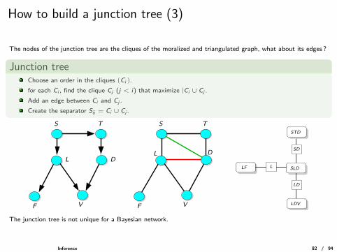
How to build a junction tree (3)
The nodes of the junction tree are the cliques of the moralized and triangulated graph, what about its edges ?
Junction treeChoose an order in the cliques (Ci).
for each Ci , find the clique Cj (j < i) that maximize |Ci ∪ Cj .
Add an edge between Ci and Cj .
Create the separator Sij = Ci ∪ Cj .
V
S T
L
F
DL
S T
F V
D
LD
SD
L
LDV
SLD
STD
LF
The junction tree is not unique for a Bayesian network.
Inference 82 / 94
Potentials
V
S T
L
F
DL
S T
F V
D
LD
SD
L
LDV
SLD
STD
LF
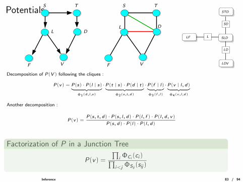
Decomposition of P(V ) following the cliques :
P(v) = P(s) · P(l | s)︸ ︷︷ ︸φ1(d,l,s)
·P(t | s) · P(d | t)︸ ︷︷ ︸φ2(s,t,d)
·P(f | l)︸ ︷︷ ︸φ3(f ,l)
·P(v | l, d)︸ ︷︷ ︸φ4(v,l,d)
Another decomposition :
P(v) =P(s, t, d) · P(s, l, d) · P(l, f ) · P(l, d, v)
P(s, d) · P(l) · P(l, d)
Factorization of P in a Junction Tree
P(v) =
∏i ΦCi (ci )∏
i<j ΦSij (sij)
Inference 83 / 94
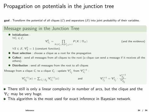
Propagation on potentials in the junction tree
goal : Transform the potential of all cliques (C) and separators (S) into joint probability of their variables.
Message passing in the Junction TreeInitialization :∀Ci ∈ C,
Ψ0Ci
=∏
X∈Ci ,X /∈Cj ,j<i
P(X | ΠX ) (and the evidence)
∀S ∈ S, Ψ0S = 1 (constant function).
Root selection : choose a clique as a root for the propagation
Collect : send all messages from all cliques to the root (a clique can send a message if it receives all theothers).
Distribution : send all messages from the root to all cliques
Message from a clique Ci to a clique Cj : update ΨtCj
from Ψt+1Ci
:
Ψt+1Sij
(s) =∑
Ci\SijΨt+1
Ci(c) and Ψt+1
Cj= Ψt
Cj·Ψt+1
Sij
ΨtSij
There still is only a linear complexity in number of arcs, but the clique and theΨC may be very huge.
This algorithm is the most used for exact inference in Bayesian network.
Inference 84 / 94
Copulas Bayesian Network
Inference 85 / 94
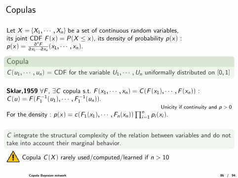
Copulas
Let X = {X1, · · · ,Xn} be a set of continuous random variables,its joint CDF F (x) = P(X ≤ x), its density of probability p(x) :p(x) = ∂nF
∂x1···∂xn (x1, · · · , xn).
Copula
C (u1, · · · , un) = CDF for the variable U1, · · · ,Un uniformally distributed on [0, 1]
Sklar,1959 ∀F , ∃C copula s.t. F (x1, · · · , xn) = C (F (x1), · · · ,F (xn)) :C (u) = F (F−1
1 (u1), · · · ,F−11 (un)).
Unicity if continuity and p > 0
For the density : p(x) = c(F1(x1), · · · ,Fn(xn))∏n
i=1 pi (xi ).
C integrate the structural complexity of the relation between variables and do nottake into account their marginal behavior.
Copula C (X ) rarely used/computed/learned if n > 10
Copula Bayesian network 86 / 94
Copula Bayesian Networks
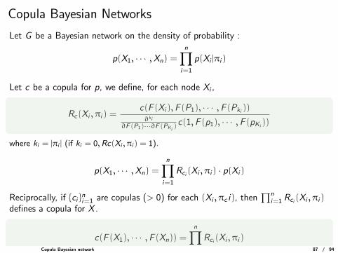
Let G be a Bayesian network on the density of probability :
p(X1, · · · ,Xn) =
n∏i=1
p(Xi |πi )
Let c be a copula for p, we define, for each node Xi ,
Rc(Xi , πi ) =c(F (Xi ),F (P1), · · · ,F (Pki ))∂ki
∂F(P1)···∂F(PKi)c(1,F (p1), · · · ,F (pKi ))
where ki = |πi | (if ki = 0,Rc(Xi , πi ) = 1).
p(X1, · · · ,Xn) =
n∏i=1
Rci (Xi , πi ) · p(Xi )
Reciprocally, if {ci }ni=1 are copulas (> 0) for each (Xi , πc i), then
∏ni=1 Rci (Xi , πi )
defines a copula for X .
c(F (X1), · · · ,F (Xn)) =
n∏i=1
Rci (Xi , πi )Copula Bayesian network 87 / 94
Copula Bayesian Network - Learning and inference
ý Definition (Copula Bayesian Network)
A CBN is described by a triplet (G , ΘC , Θp) where G is a DAG over X , ΘC is aset of copulas c(Xi , πi ), Θp is the set of marginals p(Xi ).Then the CBN has a joint density of probability p(X ) factorised by :
p(X1, · · · ,Xn) =
n∏i=1
Rci (Xi , πi ) · p(Xi )
The same properties of locality hold for CBN as for BN.
Large reduction of the number of parameters
Parameter learning can be made locally on Xi , πinot the same dataset for each Rc .not the same type of copula for each Xi , πi
Structural learning could use the same kind of algorithms than classical BN.
Inference is simpified : simulation, Rosenblatts’ transformation (etc)
Copula Bayesian network 88 / 94
Copula Junction Tree
BI
D
E
C
D
I
E
F G H
B
A
BC
EF EH
ABC BCI
BDIDE
EG
E E
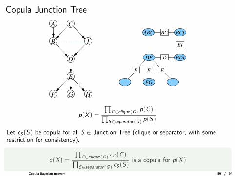
p(X ) =
∏C∈clique(G) p(C )∏
S∈separator(G) p(S)
Let cS(S) be copula for all S ∈ Junction Tree (clique or separator, with somerestriction for consistency).
c(X ) =
∏C∈clique(G) cC (C )∏
S∈separator(G) cS(S)is a copula for p(X )
Copula Bayesian network 89 / 94
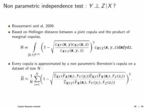
Non parametric independence test : Y |= Z |X ?
Bouezmarni and al, 2009.
Based on Hellinger distance between a joint copula and the product ofmarginal copulas,
Every copula is approximated by a non parametric Bernstein’s copula on adataset of size N :
Copula Bayesian network 90 / 94
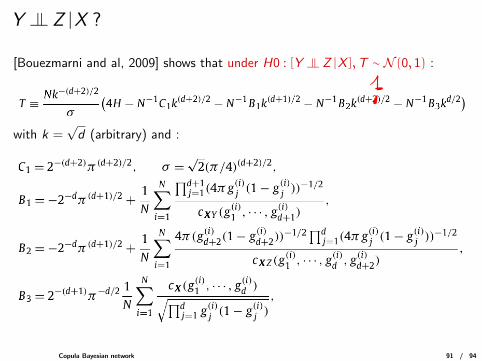
Y |= Z |X ?
[Bouezmarni and al, 2009] shows that under H0 : [Y |= Z |X ],T ∼ N (0, 1) :
with k =√d (arbitrary) and :
Copula Bayesian network 91 / 94
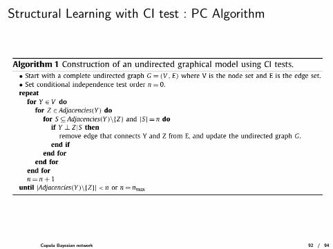
Structural Learning with CI test : PC Algorithm
Copula Bayesian network 92 / 94
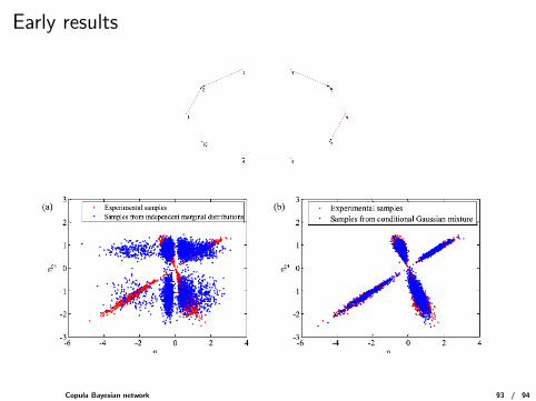
Early results
Copula Bayesian network 93 / 94
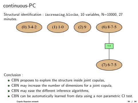
continuous-PC
Structural identification : increasing blocks, 10 variables, N=10000, 27minutes.
Conclusion :
CBN proposes to explore the structure inside joint copulas,
CBN may increase the number of dimensions for a joint copula,
CBN may ease the different inference algorithms,
CBN can be automatically learned from data using a non parametric CI test.
Copula Bayesian network 94 / 94