International Conference on Computer Systems and Technologies - CompSysTech’06

Bayesian Network Learning for Rare Events

Samuel G. Gerssen, Leon J. M. Rothkrantz

Abstract: Parameter learning from data in Bayesian networks is a straightforward task. The average number of observed occurrences is stored in a conditional probability table, from which future predictions can be calculated. This method relies heavily on the quality of the data. A data set with ‘rare events’ will not yield statistically reliable estimates. Bayesian networks allow prior and posterior learning. In this paper, new prior assessment techniques are introduced to obtain stable priors for a conditional probability table. These learning algorithms are implemented and tested, and the results will be presented.

Key words: Bayesian networks, Learning, Naive Bayes priors.

INTRODUCTION

A Bayesian network [8, 10] is a directed acyclic graph with each node representing a variable and each arc representing a causal relation between two variables. Variables are characterized by a probability distribution for each value. The probability distribution of each node is influenced by the states (for discrete nodes) or values (for continuous nodes) of the parent node. The conditional probabilities of a node are stored in a conditional probability table (CPT). The CPT is needed to calculate any conditional probability in the model, inference [5]. The size of the CPT depends on the number of states (s), the number of parents (p), and the number of parent states (sp) in the following way:

ppssCPTsize )()( ⋅= (1)

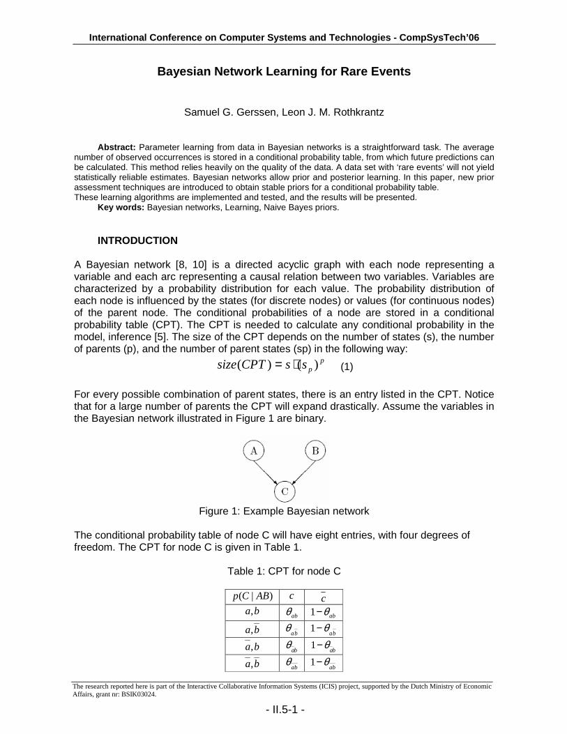
For every possible combination of parent states, there is an entry listed in the CPT. Notice that for a large number of parents the CPT will expand drastically. Assume the variables in the Bayesian network illustrated in Figure 1 are binary.

Figure 1: Example Bayesian network

The conditional probability table of node C will have eight entries, with four degrees of freedom. The CPT for node C is given in Table 1.

Table 1: CPT for node C

)|( ABCp c c ba,

abθ abθ−1

ba, baθ

baθ−1

ba, baθ

baθ−1

ba, abθ

abθ−1

The research reported here is part of the Interactive Collaborative Information Systems (ICIS) project, supported by the Dutch Ministry of Economic Affairs, grant nr: BSIK03024. - II.5-1 -

International Conference on Computer Systems and Technologies - CompSysTech’06

The number of degrees of freedom of a CPT with number of states (s), number of parents (p), and number of parent states ( ps ) is )1( −ss p

p . Values for θ can be obtained from the

data by parameter learning. abθ is the number of occurrences ( abc, ) divided by the

number of occurrences ( ab ), or ( abc, ) + ( abc, ). In general, if for a variable X, with states

Nxx ,...,1 , ip is the i-th combination of parent states, then ijθ denotes the probability of

jx given ip . Let ),( ji xpo be the number of observations ),( ji xp in the data set. ijθ can

now be calculated as follows:

�=

=N

kki

jiij

xpo

xpo

1

),(

),(θ (2)

Parameter learning is basically counting the number of observations of a specific event. Notice that the accuracy of θ heavily depends on the number of observed events. A large number of observations will result in a more accurate estimate than just a small sample. Therefore, large data sets usually provide good, stable models. Unfortunately many real-world data sets are imbalanced; some states of the response variable may be dozens to thousands of times less likely than other states. This is the case in, for example, customer bankruptcies in banks, international armed conflicts, or epidemiological infections. Thus the effect of having a large data set available is canceled by the fact that it contains only a small number of ‘interesting’ records. Therefore, a model based on such data may be severely biased or highly unstable.

PREVIOUS WORK

Rare event problems occur in generalized linear models, such as logistic regression, but also in models learned from data, such as neural networks and Bayesian networks. Especially in the case of generalized linear models, techniques such as prior correction and weighting have been developed to discard most of the ‘uninteresting’ part of the data set without much performance loss [4]. Additionally there are ways of reducing bias and variance [9]. In Bayesian networks, small sample problems are usually solved by setting a good prior distribution [1, 6], based on expert knowledge. However, if this expert knowledge is not available, an acceptable prior, based on the data, needs to be set. [7] proposes noisy-OR to obtain priors. This approach uses cutting to shift from prior to posterior estimate. Naive Bayes is a very good classifier, as described in [2]. Parameter learning is explained in detail by David Heckerman in [3]. Inference in a Bayesian network is the calculation of conditional probabilities, given the probabilities in a CPT. Inference is based on two rules. The first one is Bayes’ rule, which is defined as:

)(

)()|()|(

yp

xpxypyxp = (3)

The second rule is the expansion rule, which is defined for binary variables ( )(1)( xpxp −= ) as:

- II.5-2 -

International Conference on Computer Systems and Technologies - CompSysTech’06

��=+++=

+=

Y Z

yzpyzxp

yzpyzxpzypzyxpzypzyxpyzpyzxpxp

ypyxpypyxpxp

)()|(

)()|()()|()()|()()|()(

)()|()()|()(

(4)

Using these two rules, in the example in Figure 1, )|( cap can now be calculated:

� ��=

=

Aab)p(ab) | p(c

ab)p(b) | p(c)(

)(

)|()()|(

B

Bap

cp

acpapcap

(5)

Inference will be used for the assessment of naive Bayes priors.

CPT Calculation Deriving CPT parameters using a prior-posterior approach consists of three stages:

1. prior assessment 2. posterior assessment 3. merging

The posterior assessment is equivalent with CPT parameter learning, shown in equation 2, and will not be discussed here. First, the merging method is described and then the prior assessment. Merging The merging process of priors and posteriors can be handled in a couple of ways. [7] uses a cut value for the number of observations, in that paper called smoothing. If, in the data set, a combination of parent states pi occurs less than the cut value, the prior will be used in the CPT. Otherwise, the posterior will be used. Let the prior for ijθ be ijp , the posterior

ijr , and the cut value c, the smoothing merging is defined as:

��

��

� <= �=otherwiser

ifp

ij

ijij

,

c ) x,o(p,N

1kkiθ (6)

Substitution of equations 2 and 6 yields:

��

�

��

�

� <

=

�

�

=

=

otherwise

ifp

N

k

ij

ij ,) x,o(p

) x,o(p

c ) x,o(p,

1ki

ji

j

1kki

θ (7)

- II.5-3 -

International Conference on Computer Systems and Technologies - CompSysTech’06

In this paper, a gentle transition is proposed, by weighting the priors. The priors will receive an integer value, weight w, which is equivalent to a number of observations. The resulting CPT entries will be a weighted average of the priors and the posteriors:

�=

+

+=

j

k

ij

1ki

jiij

) x,o(p w

) x,o(p )p · (wθ (8)

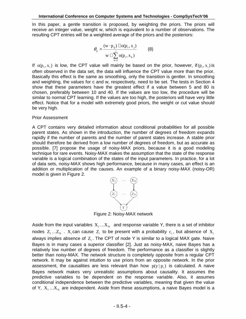
If ) x,o(p ii is low, the CPT value will mainly be based on the prior, however, if ) x,(p ii is often observed in the data set, the data will influence the CPT value more than the prior. Basically this effect is the same as smoothing, only the transition is gentler. In smoothing and weighting, the values for c and w, respectively, need to be set. The tests in Section 4 show that these parameters have the greatest effect if a value between 5 and 80 is chosen, preferably between 10 and 40. If the values are too low, the procedure will be similar to normal CPT learning. If the values are too high, the posteriors will have very little effect. Notice that for a model with extremely good priors, the weight or cut value should be very high. Prior Assessment A CPT contains very detailed information about conditional probabilities for all possible parent states. As shown in the introduction, the number of degrees of freedom expands rapidly if the number of parents and the number of parent states increase. A stable prior should therefore be derived from a low number of degrees of freedom, but as accurate as possible. [7] propose the usage of noisy-MAX priors, because it is a good modeling technique for rare events. Noisy-MAX makes the assumption that the state of the response variable is a logical combination of the states of the input parameters. In practice, for a lot of data sets, noisy-MAX shows high performance, because in many cases, an effect is an addition or multiplication of the causes. An example of a binary noisy-MAX (noisy-OR) model is given in Figure 2.

Figure 2: Noisy-MAX network

Aside from the input variables .X . . X N1 and response variable Y, there is a set of inhibitor

nodes .Z . . Z N1 . iX can cause iZ to be present with a probability ic , but absence of iX

always implies absence of iZ . The CPT of node Y is similar to a logical MAX gate. Naive Bayes is in many cases a superior classifier [2]. Just as noisy-MAX, naive Bayes has a relatively low number of degrees of freedom. The performance as a classifier is slightly better than noisy-MAX. The network structure is completely opposite from a regular CPT network. It may be against intuition to use priors from an opposite network. In the prior assessment, the causalities are less relevant than how )p|p(y i is calculated. A naive Bayes network makes very unrealistic assumptions about causality. It assumes the predictive variables to be dependent on the response variable. Also, it assumes conditional independence between the predictive variables, meaning that given the value of Y, .X . . X N1 are independent. Aside from these assumptions, a naive Bayes model is a

- II.5-4 -

International Conference on Computer Systems and Technologies - CompSysTech’06

very powerful classifier. Inference in a naive Bayes network is not as straightforward as in a CPT network. A network with predictive variables .X . . X N1 and response variable Y with

states .y . . y M1 will have the probabilities )p|p(y i listed in the CPT. In a naive Bayes network, these values need to be calculated as follows:

∏�

∏∏

∏

=

=

=

i jjji

ii

ii

ii

i

i

ypyxp

ypyxp

xp

ypyxp

pp

ypypp

))()|((

)()|(

)(

)()|(

)(

)()|()p|p(y i

(9)

The values for )|p(xi y and p(y) can be obtained by parameter learning in the naive Bayes network. ijp from equation 8 can be replaced by the right part of equation 9. Now the

formula for calculation of the CPT values is complete. RESULTS

The method above was implemented and tested on a bankruptcy data set from a bank. The bankruptcies were rare (around 2% of all records). As a performance measure for scoring the models, the GINI index was used. In a graph where a curve is plotted as the cumulative bankrupt percentage of clients against the total percentage of clients when they are sorted on risk (low risk on the left, high risk on the right), the GINI index is defined as the area between the diagonal and the curve (the Lorentz curve) divided by the total area under the diagonal. It has a range between -1 and 1, or −100% to 100%. High scores indicate good models. The GINI index is widely used in social sciences to measure the discriminative power of a model.

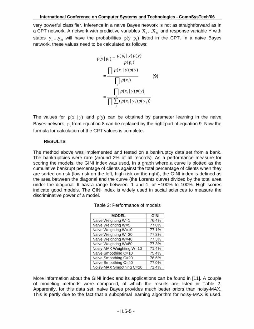
Table 2: Performance of models

MODEL GINI Naive Weighting W=1 76.4% Naive Weighting W=5 77.0% Naive Weighting W=10 77.1% Naive Weighting W=20 77.2% Naive Weighting W=40 77.3% Naive Weighting W=80 77.3% Noisy-MAX Weighting W=10 71.4% Naive Smoothing C=10 75.4% Naive Smoothing C=20 76.6% Naive Smoothing C=40 77.0% Noisy-MAX Smoothing C=20 71.4%

More information about the GINI index and its applications can be found in [11]. A couple of modeling methods were compared, of which the results are listed in Table 2. Apparently, for this data set, naive Bayes provides much better priors than noisy-MAX. This is partly due to the fact that a suboptimal learning algorithm for noisy-MAX is used.

- II.5-5 -

International Conference on Computer Systems and Technologies - CompSysTech’06

Even with EM learning, noisy-MAX scores will not be higher than 76%. Secondly, the weighting seems to perform better than the smoothing for this data set.

CONCLUSIONS AND FUTURE WORK

Two improvements to learning for rare event data were suggested in this paper. Firstly, weighted merging instead of cutting, which allows a more gentle balance between a prior and a posterior. Secondly, inference in a naive Bayes models can provide excellent priors for a CPT in a ‘normal’ Bayesian network. Compared to existing methods, such as noisy-MAX priors, naive Bayes priors perform better on the test data set. Unfortunately, the best performing model on this data set was naive Bayes without any posterior learning. Therefore, more data sets to test these methods on are required for a definite statement. These initial results are very promising.

REFERENCES [1] Beck, N., G. King & L. Zeng. ‘The Problem with Quantitative Studies of

International Conflict.’ http://web.polmeth.ufl.edu/papers/98/beck98.zip. [2] Friedman, N., D. Geiger & M. Goldszmidt. ‘Bayesian Network Classifiers.’ Machine

Learning 29(2-3):131-163, 1997. [3] Heckerman, D. ‘A Tutorial on Learning Bayesian Networks.’ Technical Report,

Microsoft Research, 1995. [4] King, G. & L. Zeng. ‘Logistic Regression in Rare Events Data.’ Political Analysis

9(2):137-163, 2001. [5] Lauritzen, S.L. & D.J. Spiegelhalter. ‘Local computations with probabilities on

graphical structures and their application to expert systems (with discussion).’ Journal of Royal Statistical Society, Series B 50(2):157-224, 1988.

[6] Neal, R.M. Bayesian Learning for Neural Networks. Springer-Verlag, 1996. [7] Onisko, A., M.J. Druzdzel & H. Wasyluk. ‘Learning Bayesian network parameters

from small data sets: application of Noisy-OR gates.’ International Journal of Approximate Reasoning 27(2):165-182, 2001.

[8] Pearl, J. Probabilistic Reasoning in Intelligent Systems: Networks of Plausible Inference. Morgan Kaufmann, 1988.

[9] Ripley, B.D. Pattern Recognition and Neural Networks. Cambridge University Press, 1996.

[10] Spirtes, P., C. Glymour & R. Scheines Causation, Prediction and Search. Lecture Notes in Statistics 81, Springer Verlag, 1993.

[11] Xu, K. ‘How has the literature on Gini’s Index evolved in the past 80 years?’ Working paper, 2003.

ABOUT THE AUTHOR Assoc. Prof. L. J. M. Rothkrantz, Department of Man-Machine Interaction, Delft University of Technology, Phone: +31 15 2787504,

�-mail: L.J.M.Rothkrantz@ewi.tudelft.nl

- II.7-3 -

- II.5-6 -