Embed Size (px)
Citation preview
Language, Cognition, and Mind
Bayesian Natural Language Semantics and Pragmatics
Henk ZeevatHans-Christian Schmitz Editors

Language, Cognition, and Mind
Volume 2
Series editor
Chungmin Lee, Seoul National University, Seoul, South Korea
Editorial board members
Tecumseh Fitch, University of Vienna, Vienna, AustriaPeter Gaerdenfors, Lund University, Lund, SwedenBart Geurts, Radboud University, Nijmegen, The NetherlandsNoah D. Goodman, Stanford University, Stanford, USARobert Ladd, University of Edinburgh, Edinburgh, UKDan Lassiter, Stanford University, Stanford, USAEdouard Machery, Pittsburgh University, Pittsburgh, USA

This series takes the current thinking on topics in linguistics from the theoreticallevel to validation through empirical and experimental research. The volumespublished offer insights on research that combines linguistic perspectives fromrecently emerging experimental semantics and pragmatics as well as experimentalsyntax, phonology, and cross-linguistic psycholinguistics with cognitive scienceperspectives on linguistics, psychology, philosophy, artificial intelligence andneuroscience, and research into the mind, using all the various technical and criticalmethods available. The series also publishes cross-linguistic, cross-cultural studiesthat focus on finding variations and universals with cognitive validity. The peerreviewed edited volumes and monographs in this series inform the reader of theadvances made through empirical and experimental research in the language-related cognitive science disciplines.
More information about this series at http://www.springer.com/series/13376

Henk Zeevat • Hans-Christian SchmitzEditors
Bayesian Natural LanguageSemantics and Pragmatics
123

EditorsHenk ZeevatILLCUniversity of AmsterdamAmsterdamThe Netherlands
Hans-Christian SchmitzFraunhofer Institute for CommunicationInformation Processing and ErgonomicsFKIE
WachtbergGermany
ISSN 2364-4109 ISSN 2364-4117 (electronic)Language, Cognition, and MindISBN 978-3-319-17063-3 ISBN 978-3-319-17064-0 (eBook)DOI 10.1007/978-3-319-17064-0
Library of Congress Control Number: 2015939421
Springer Cham Heidelberg New York Dordrecht London© Springer International Publishing Switzerland 2015This work is subject to copyright. All rights are reserved by the Publisher, whether the whole or partof the material is concerned, specifically the rights of translation, reprinting, reuse of illustrations,recitation, broadcasting, reproduction on microfilms or in any other physical way, and transmissionor information storage and retrieval, electronic adaptation, computer software, or by similar or dissimilarmethodology now known or hereafter developed.The use of general descriptive names, registered names, trademarks, service marks, etc. in thispublication does not imply, even in the absence of a specific statement, that such names are exempt fromthe relevant protective laws and regulations and therefore free for general use.The publisher, the authors and the editors are safe to assume that the advice and information in thisbook are believed to be true and accurate at the date of publication. Neither the publisher nor theauthors or the editors give a warranty, express or implied, with respect to the material contained herein orfor any errors or omissions that may have been made.
Printed on acid-free paper
Springer International Publishing AG Switzerland is part of Springer Science+Business Media(www.springer.com)

Preface
Natural language interpretation (NLI) can be modelled analogously to Bayesiansignal processing: the most probable message M (corresponding to the speaker’sintention) conveyed by a signal S (a word, a sentence, turn or text) is found by twomodels, namely the prior probability of the message and the production probabilityof the signal. From these models and Bayes’ theorem, the most probable messagegiven the signal can be derived. Although the general capacity of Bayesian modelshas been proven in disciplines like artificial intelligence, cognitive science, com-putational linguistics and signal processing, they are not yet common in NLI.
Bayesian NLI gives three departures from standard assumptions. First, it can beseen as a defence of linguistic semantics as a production system that maps meaningsinto forms as was assumed in generative semantics, but also in systemic grammar,functional grammar and optimality theoretic syntax. This brings with it a morerelaxed view of the relation between syntactic and semantic structures; the mappingfrom meanings to forms should be efficient (linear) and the prior strong enough tofind the inversion from the cues in the utterance.
The second departure is that the prior is also the source for what is not said in theutterance but part of the pragmatic enrichment of the utterance: what is part of thespeaker intention but not of the literal meaning. There is no principled differencebetween inferring in perception that the man who is running in the direction of thebus stop as the bus is approaching is trying to catch the bus and inferring inconversation that the man who states that he is out of petrol is asking for help withhis problem.
The third departure is thus that interpretation is viewed as a stochastic andholistic process leading from stochastic data to a symbolic representation or aprobability distribution over such representations that can be equated with theconversational contribution of the utterance.
Models relevant to the prior (the probability of the message M) include Bayesiannetworks for causality, association between concepts and (common ground)expectations. It is tempting to see a division in logic: classical logic for expressingthe message, the logic of uncertainty for finding out what those messages are.Radical Bayesian interpretation can be described as the view that not just the
v

identification of the message requires Bayesian methods, but also the message itselfand the contextual update have to be interpreted with reference to Bayesian beliefrevision, Bayesian networks or conceptual association.
The papers in this volume, which is one of the first on Bayesian NLI, approachthe topic from diverse angles. The following gives some minimal guidance withrespect to the content of the papers.
• Henk Zeevat: “Perspectives on Bayesian Natural Language Semantics andPragmatics” Zeevat gives an overview of the different concepts of Bayesianinterpretation and some possible applications and open issues. This paper can beread as an introduction to Bayesian NL Interpretation.
• Anton Benz: “Causal Bayesian Networks, Signalling Games and Implicature of‘More Than n’”. Benz applies Causal Bayesian Nets and signalling games toexplain the empirical data on implicatures arising from ‘more than n’ bymodelling the speaker with these nets.
• Satoru Suzuki: “Measurement-Theoretic Foundations of Logic for BetterQuestions and Answers” The paper is concerned with finding a qualitativemodel of reasoning about optimal questions and makes a promising proposal. Itis part of a wider programme to find qualitative models of other reasoning tasksthat are normally approached by numerical equations like the stochasticreasoning in Bayesian interpretation.
• Stefan Kaufmann: “Conditionals, Conditional Probabilities, andConditionalization” Kaufman gives a logical analysis of the relation betweenthe probability of a conditional and the corresponding conditional probability,proposing Bayes’ theorem as the link.
• Christian Wurm: “On the Probabilistic Notion of Causality: Models andMetalanguages” Wurm addresses the well-known problem of the reversibility ofBayesian nets. Nets can be turned into equally other nets by reversing all thearrows.
• Mathias Winther Madsen: “Shannon Versus Chomsky: Brain Potentials and theSyntax-Semantics Distinction” Based on a large number of existing experi-mental results, Madsen argues for a simple information theoretic hypothesisabout the correlates of N400 and P600 effects in which an N400 is the sign of atemporary loss of hypotheses and a P600 the sign of too many hypotheses. Thisinformation theoretic approach has a strong relation with incremental Bayesianinterpretation.
• Jacques Jayez: “Orthogonality and Presuppositions: A Bayesian Perspective”Jayez gives a direct application of Bayesian interpretation to the differentialbehaviour of various presupposition triggers in allowing presuppositionsuspension.
• Grégoire Winterstein: “Layered Meanings and Bayesian Argumentation: TheCase of Exclusives” Winterstein applies a Bayesian theory of argumentation tothe analysis of exclusive particles like “only”.
• Ciyang Qing and Michael Franke: “Variations on a Bayesian Theme: ComparingBayesian Models of Referential Reasoning” Inspired by game-theoretical
vi Preface

pragmatics, Qing and Franke propose a series of improvements to the RSAmodelof Goodman and Frank with the aim of improving its predictive power.
• Peter R. Sutton: “Towards a Probabilistic Semantics for Vague Adjectives”Sutton formalises and defends a nominalist approach to vague predicatesin situation theory in which Bayesian learning is directly responsible forlearning the use and interpretation of such predicates without an interveninglogical representation.
The volume grew out of a workshop on Bayesian Natural Language Semanticsand Pragmatics, held at the European Summer School of Logic, Language andInformation (ESSLLI) 2013 in Düsseldorf. We would like to thank all the workshopparticipants for their contributions to the success of the workshop and the qualityof the papers in this volume. Furthermore, we thank the members of the programmecommittee, Anton Benz, Graeme Forbes, Fritz Hamm, Jerry Hobbs, NoahGoodman, Gerhard Jäger, Jacques Jayez, Stefan Kaufmann, Uwe Kirschenmann,Ewan Klein, Daniel Lassiter, Jacob Rosenthal, Remko Scha, David Schlangen,Markus Schrenk, Bernhard Schröder, Robert van Rooij, Grégoire Winterstein andThomas Ede Zimmermann, for their help in selecting suitable contributions. Wealso owe thanks to the series editor Chungmin Lee, to Helen van der Stelt ofSpringer and to the anonymous reviewers who helped out in the reviewing andselection process. Last but not least, we thank the German Society forComputational Linguistics & Language Technology (GSCL) for its financial sup-port of the workshop.
Henk ZeevatHans-Christian Schmitz
Preface vii
Contents
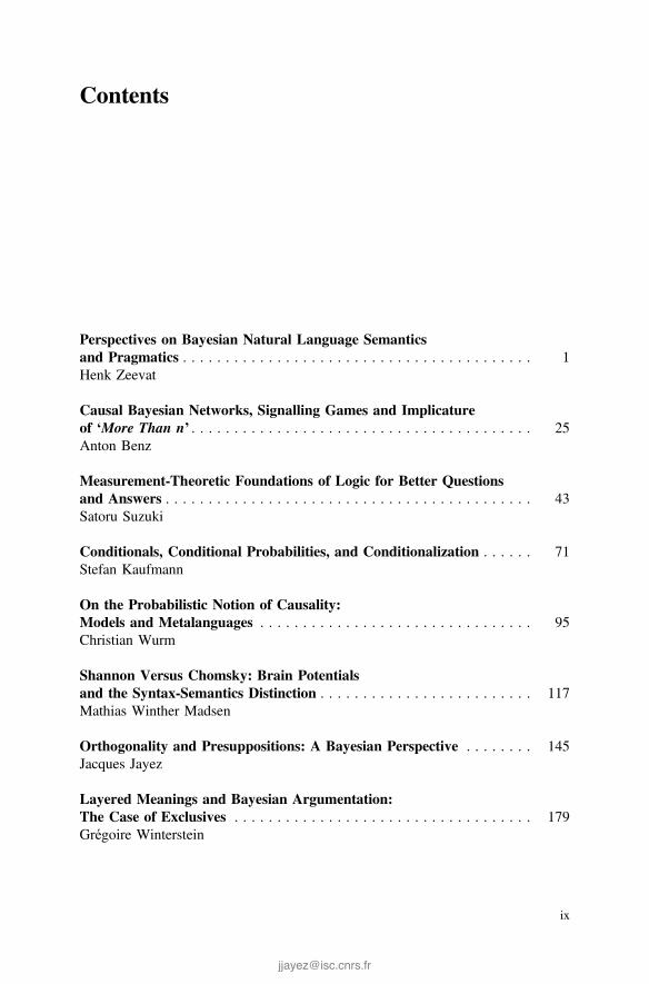
Perspectives on Bayesian Natural Language Semanticsand Pragmatics . . . . . . . . . . . . . . . . . . . . . . . . . . . . . . . . . . . . . . . . . 1Henk Zeevat
Causal Bayesian Networks, Signalling Games and Implicatureof ‘More Than n’ . . . . . . . . . . . . . . . . . . . . . . . . . . . . . . . . . . . . . . . . 25Anton Benz
Measurement-Theoretic Foundations of Logic for Better Questionsand Answers . . . . . . . . . . . . . . . . . . . . . . . . . . . . . . . . . . . . . . . . . . . 43Satoru Suzuki
Conditionals, Conditional Probabilities, and Conditionalization . . . . . . 71Stefan Kaufmann
On the Probabilistic Notion of Causality:Models and Metalanguages . . . . . . . . . . . . . . . . . . . . . . . . . . . . . . . . 95Christian Wurm
Shannon Versus Chomsky: Brain Potentialsand the Syntax-Semantics Distinction . . . . . . . . . . . . . . . . . . . . . . . . . 117Mathias Winther Madsen
Orthogonality and Presuppositions: A Bayesian Perspective . . . . . . . . 145Jacques Jayez
Layered Meanings and Bayesian Argumentation:The Case of Exclusives . . . . . . . . . . . . . . . . . . . . . . . . . . . . . . . . . . . 179Grégoire Winterstein
ix

Variations on a Bayesian Theme: Comparing BayesianModels of Referential Reasoning . . . . . . . . . . . . . . . . . . . . . . . . . . . . 201Ciyang Qing and Michael Franke
Towards a Probabilistic Semantics for Vague Adjectives . . . . . . . . . . . 221Peter R. Sutton
x Contents
Contributors
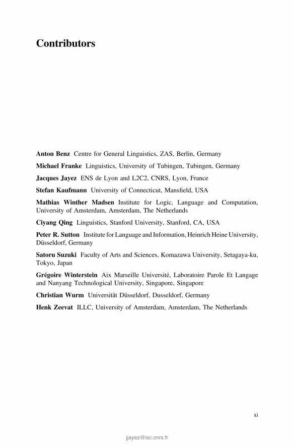
Anton Benz Centre for General Linguistics, ZAS, Berlin, Germany
Michael Franke Linguistics, University of Tubingen, Tubingen, Germany
Jacques Jayez ENS de Lyon and L2C2, CNRS, Lyon, France
Stefan Kaufmann University of Connecticut, Mansfield, USA
Mathias Winther Madsen Institute for Logic, Language and Computation,University of Amsterdam, Amsterdam, The Netherlands
Ciyang Qing Linguistics, Stanford University, Stanford, CA, USA
Peter R. Sutton Institute for Language and Information, Heinrich Heine University,Düsseldorf, Germany
Satoru Suzuki Faculty of Arts and Sciences, Komazawa University, Setagaya-ku,Tokyo, Japan
Grégoire Winterstein Aix Marseille Université, Laboratoire Parole Et Langageand Nanyang Technological University, Singapore, Singapore
Christian Wurm Universität Düsseldorf, Dusseldorf, Germany
Henk Zeevat ILLC, University of Amsterdam, Amsterdam, The Netherlands
xi

Perspectives on Bayesian Natural LanguageSemantics and Pragmatics
Henk Zeevat
Abstract Bayesian interpretation is a technique in signal processing and itsapplication to natural language semantics and pragmatics (BNLSP from here onand BNLI if there is no particular emphasis on semantics and pragmatics) is basi-cally an engineering decision. It is a cognitive science hypothesis that humans emu-late BNLSP. That hypothesis offers a new perspective on the logic of interpretationand the recognition of other people’s intentions in inter-human communication. Thehypothesis also has the potential of changing linguistic theory, because the mappingfrom meaning to form becomes the central one to capture in accounts of phonology,morphology and syntax. Semantics is essentially read off from this mapping andpragmatics is essentially reduced to probability maximation within Grice’s intentionrecognition. Finally, the stochastic models used can be causal, thus incorporatingnew ideas on the analysis of causality using Bayesian nets. The paper explores andconnects these different ways of being committed to BNLSP.
Keywords Bayesian interpretation · Semantics · Pragmatics · Stochastic naturallanguage interpretation · Presupposition · Implicature
Overview
This paper explains six ways in which one can understand the notion of BayesianNatural Language Semantics and Pragmatics and argues for each of them that theymerit consideration since they seem to allow progress in understanding human lan-guage interpretation and with respect to problems in the area of NL semantics andpragmatics. The six ways can be listed as in (1).
H. Zeevat (B)ILLC, University of Amsterdam, Amsterdam, The Netherlandse-mail: [email protected]
© Springer International Publishing Switzerland 2015H. Zeevat and H.-C. Schmitz (eds.), Bayesian Natural Language Semanticsand Pragmatics, Language, Cognition, and Mind 2,DOI 10.1007/978-3-319-17064-0_1
1
2 H. Zeevat
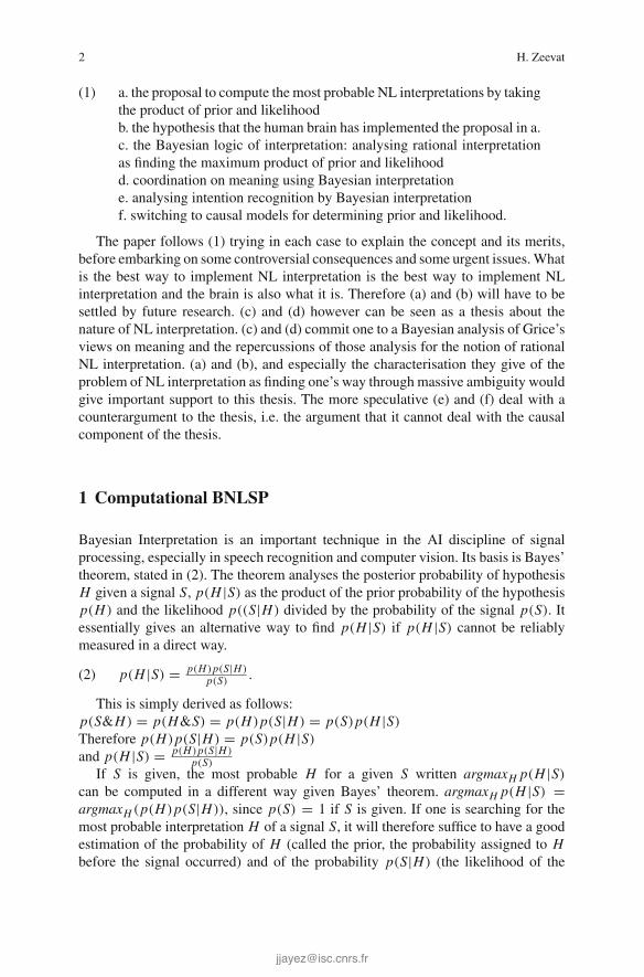
(1) a. the proposal to compute the most probable NL interpretations by takingthe product of prior and likelihoodb. the hypothesis that the human brain has implemented the proposal in a.c. the Bayesian logic of interpretation: analysing rational interpretationas finding the maximum product of prior and likelihoodd. coordination on meaning using Bayesian interpretatione. analysing intention recognition by Bayesian interpretationf. switching to causal models for determining prior and likelihood.
The paper follows (1) trying in each case to explain the concept and its merits,before embarking on some controversial consequences and some urgent issues.Whatis the best way to implement NL interpretation is the best way to implement NLinterpretation and the brain is also what it is. Therefore (a) and (b) will have to besettled by future research. (c) and (d) however can be seen as a thesis about thenature of NL interpretation. (c) and (d) commit one to a Bayesian analysis of Grice’sviews on meaning and the repercussions of those analysis for the notion of rationalNL interpretation. (a) and (b), and especially the characterisation they give of theproblem of NL interpretation as finding one’s way through massive ambiguity wouldgive important support to this thesis. The more speculative (e) and (f) deal with acounterargument to the thesis, i.e. the argument that it cannot deal with the causalcomponent of the thesis.
1 Computational BNLSP
Bayesian Interpretation is an important technique in the AI discipline of signalprocessing, especially in speech recognition and computer vision. Its basis is Bayes’theorem, stated in (2). The theorem analyses the posterior probability of hypothesisH given a signal S, p(H |S) as the product of the prior probability of the hypothesisp(H) and the likelihood p((S|H) divided by the probability of the signal p(S). Itessentially gives an alternative way to find p(H |S) if p(H |S) cannot be reliablymeasured in a direct way.
(2) p(H |S) = p(H)p(S|H)p(S)
.
This is simply derived as follows:p(S&H) = p(H&S) = p(H)p(S|H) = p(S)p(H |S)
Therefore p(H)p(S|H) = p(S)p(H |S)
and p(H |S) = p(H)p(S|H)p(S)
If S is given, the most probable H for a given S written argmaxH p(H |S)
can be computed in a different way given Bayes’ theorem. argmaxH p(H |S) =argmaxH (p(H)p(S|H)), since p(S) = 1 if S is given. If one is searching for themost probable interpretation H of a signal S, it will therefore suffice to have a goodestimation of the probability of H (called the prior, the probability assigned to Hbefore the signal occurred) and of the probability p(S|H) (the likelihood of the

Perspectives on Bayesian Natural Language Semantics and Pragmatics 3
signal given the interpretation). This way of finding the most probable H is usefuland often unavoidable, since it can be difficult or even impossible to directly estimatep(H |S) (the posterior probability of the interpretation H , after the occurrence of thesignal S).
The difficulty for direct estimation is especially clear when the set of signals isinfinite or continuous, as in speech perception or in vision. For example, in speechperception, onemeasures the distance between the perceived signal and the predictedsignal to estimate likelihood and uses the prediction for the next phoneme from thepreceding phoneme sequence obtained from a large body of written text to estimatethe prior.
The definition just givenmakesBNLI a specialway of obtaining themost probableinterpretation of an utterance and BNLI is thereby a branch of stochastic signalinterpretation.
One needs a good argument for usingBayesian interpretation rather than the directmethod of estimating the posterior. And one needs to accept that natural language isambiguous to go stochastic in the first place.
The method by itself does not entail that both likelihood and prior need to beestimated stochastically. The prior can be partly computed by symbolic techniques,e.g. by a theorem prover showing that the prior is not 0 by showing the consistencyof the interpretation with the context. Similarly, one can use symbolic techniques(e.g. a text generator in NLI—these are standardly symbolic) to estimate likelihood.
Doing NLI or NLSP with this technique makes BNLSP a branch of stochasticNLSP. Stochastic NLSP obviously helps in obtaining good results in interpretation,since NL utterances severely underdetermine their interpretations in context andother techniques for disambiguation are limited in scope. It is also easy to see thatvery often disambiguation cannot be explained by an appeal to hard facts and logic,but needs to appeal to what is probable in the world. For example, if I tell you that Itook the bus, you will understand me as having used the public transport system andnot as having lifted an autobus with my crane. Another basic example is (3).
(3) Tweety flies.
If you are like me, Tweety is the bird from AI discussions about default reasoningand “flies” means “can fly using his wings”. There must be many other Tweetieshowever and there is no logical reason why the verbal form could not mean “usesaeroplanes” or “can pilot aeroplanes”.
The underdetermination of meaning by form can be argued by looking at anybranch of linguistic description. The most obvious and most traditional place is thelexicon. Non-ambiguous words are rare to non-existent. Chomsky’s proposals forsyntax brought syntactic ambiguity to the centre of attention. Formal treatmentsof phonology and morphology have also led to phonological and morphologicalambiguity, while the semantics of morphemes makes them much more ambiguousthan proper lexical items. Montague grammar initially concentrated on quantifierscope ambiguities. But this is just another instance of semantic relations that remainunmarked in syntax. Famous examples in English are noun-noun combinations and

4 H. Zeevat
the semantic relation to the main clause as marked by a participial construction.Areas of pragmatics that can be described as “ambiguous” are pronoun resolution,the recognition of rhetorical relations, temporal reference resolution, exhaustivityand stereotypicality effects and the treatment of presuppositions.
It follows that success in NLSP can only be expected by viable approaches toselection of interpretations, an aspect of the form-meaning relation which is stillneglected with respect to the composition of meaning within semantics and prag-matics.
Ambiguity adds up to an argument for stochastic NLI. But not necessarily to anargument for Bayesian NLI. Within the confines of stochastic NLI there is anotherhypothesis possible, the direct method in which a system of hierarchically organisedcues directly leads to the most probable meaning. It is not directly obvious that thiscannot work for NLI. In stochastic parsing for example there have been successfulmodels based on direct estimation.
We will look at some evidence about human NLI and will argue that human BNLIis the most plausible hypothesis explaining that evidence. From that hypothesis, anargument can be constructed against the direct method in computational NLI.
2 Human BNLSP
In cognitive science, BNLSP can be seen as the claim that humans emulate BNLSPwhen they are interpreting language utterances.
There are general grounds for believing that this is the case. Some (Oaksford andChater 2007; the contributions in Doya et al. 2007; Kilner et al. 2007) speak of anemerging consensus that Bayesian reasoning is the logic of the brain—even thoughthere is also considerable opposition to this view (e.g. Bowers and Davis 2012). Suchan emerging consensus builds on successes of Bayesian analyses in major areas ofcognitive science such as inference, vision and learning. It would follow from theimportance of Bayesian reasoning in the brain that it is unlikely that human NLIwould employ a different logic.
The same point can also be made by developing the analogy between vision andNLI. Visual cues are highly ambiguous and the standard procedure in automaticvision is based on the availability of a powerful model of likelihood: the translationof the hypothesis into properties of the signal by means of the “mental camera”.Together with powerful priors about what can be perceived this gives a way to findthe most probable hypotheses among the ones that are made available by cueing.
Human language interpreters have a device much like the mental camera in theirability to translate communicative intentions into natural language utterances. Inaddition, most of the priors for vision are directly usable in NLI. It follows that theycan find the most probable interpretation for an NL utterance as reliably as theycan find the most probably perceived scene for a visual signal. In sum, there is noobstacle for assuming that human NLI has the same architecture as human vision anda strong evolutionary argument for assuming that the architecture of human vision

Perspectives on Bayesian Natural Language Semantics and Pragmatics 5
and the priors involved were exapted for the emerging human NLI.1 This would bethe simplest way in which the problem of NLI could be solved by the brain. Given theshort time frame in which NL and NLI emerged, a completely different architecturelike symbolic parsing would be difficult to achieve in evolution.
If we accept the conclusion, there is an aspect of interpretation that is not predictedby the direct cueingmodel: the role of the priors. The priors shared with vision wouldbe generalisations aboutwhat is going on in theworld to the degree that it is accessibleto normal perception. Such priors can be seen as causal prediction, topographicalinformation and conceptual knowledge. Thereby they concern primarily the highestlevels of linguistic analysis: semantics and pragmatics.
For a pure hierarchical cueing model, the direct way of estimating the posterior,having the best priors on the highest level is a problem. Those priors can only helpselection at the final levels of analysis and would be relatively unimportant at thelower levels, leading to a large number of possibilities that need to be checked beforethe final level. In a Bayesian model, the high-level priors can directly predict down tothe lowest level. Themost likely prior hypothesis that is cued by the input can be usedfor simulated production that can be checked against initial segments of the input.
It would appear therefore that a causal model of production combined with priorsas for vision is the better architecture for early selection between interpretationalpossibilities.
There is also a body of empirical evidence that makes sense under a Bayesianarchitecture for natural language interpretation. Pickering andGarrod (2007) gives anoverview of evidence for the simulated production in interpretation that is predictedby Bayesian interpretation. Clark (1996) discusses conversational moves that endwith the hearer co-producing the final segment of the utterance, something that ishard to understand without assuming simulated production. As noted by Kilner et al.(2007), the activation of mirror neurons in perception of the behaviour of othersmakes good Bayesian sense: connecting to one’s own way of carrying out the samebehaviour will give access to more fine-grained prediction from the hypothesis thatcan be matched against the visual signal.
So there is a lot of evidence in favour of aBayesian architecture of human languageinterpretation. Human BNLI also supports the idea that efforts should be made toachieve computational BNLI. If one seems to understand how humans solve a prob-lem, that gives a strategy for solving the same problem on a computer. There maycertainly be good computational reasons to depart from the human solution. But inthe face of the serious imperfections of current NLI and the absence of sufficientinvestment in BNLSP, a computational case against BNLSP is just not available atthis moment.
Computational NLSP using the direct method seems to be forced into the pipelinemodel, due to the different data-sets needed for the different kinds of processing. Apipeline model using the corpus-based methods of current stochastic parsing would
1Symbolic parsing with visual grammars becomes intractable as soon as the grammar becomesinteresting (Marriott and Meyer 1997). It follows that visual recognition must be stochastic. Toprofit fully from the mental camera, it must also be Bayesian.

6 H. Zeevat
be an alternative model for human NLI. It would involve finding the most probablesyntactic tree, followed by finding the most probable interpretation of the words inthat tree, followed by the best proto-logical form, followed by the best fully resolvedlogical form and its most probable integration in the context. The problem is simplythat a 0.8 success score on each of the levels (roughly the result for accuracy instochastic parsing) translates into a 0.85 = 0.328 score for the full pipeline, verymuch below human performance.
Bayesian models escape from this problem by assuming a causal model of utter-ance production that works in conjunction with a heuristic cueing system. If thehigh-level priors are strong enough and the causal model is accurate and sufficientlydeterministic, the combination has a much higher chance of reaching the most proba-ble interpretation. The direct method is not eliminated in this set-up since it is neededfor defining the cueing system and also because it could count as a baseline, that isimproved by the causal model. The causal model of production seemsmore adequatehowever for evaluating linguistic knowledge in the process.
3 BNLSP as the Logic of Interpretation
The logic of interpretation in Montague grammar is just classical logic augmentedby a theory of abstraction and function application. It does not deal with uncertainty.Boole developed his Boolean logic from the broader perspective of a logic thatcombines classical reasoning with reasoning about probabilities. In making BNLSPthe logic of interpretation, one restores the Boolean view of logic to deal with theuncertainty about what a particular word or phrase means on a particular occasion.
If one takes the selection problem seriously and accepts the rationality of tryingto solve it by probability maximation, BNLSP offers a promising starting pointfor the analysis of semantics and pragmatics. There is little choice about takingthe selection problem seriously. As noted above, modern linguistics can be readas an overwhelming case for the underdetermination of meaning by form and agood deal of the evidence comes precisely from the philosophical exploration ofpresupposition, thematic roles, implicature and discourse relations. To doubt therationality of probabilistic disambiguation is a way of doubting rationality as such,given that stochastically based disambiguation is needed for the interpretation ofnearly any utterance.
BNLSP motivates some simple principles. For a good interpretation, prior prob-ability must be properly higher than zero and likelihood must be properly higherthan zero. If another interpretation has the same likelihood, it must have a lowerprior. If another interpretation has the same prior, it must have a lower likelihood.These are powerful principles that can explain important aspects of interpretation.The following are some examples of their application.
Perspectives on Bayesian Natural Language Semantics and Pragmatics 7
Gricean Maxims
The simple BNLSP principles have a different status from Gricean pragmatics, sincethey are merely consequences of stochastic disambiguation. A reduction of Griceanpragmatics to these principles is thereby a step forward since it eliminates the nor-mative account of production that is the cooperativity principle. The reduction ishowever a question of reducing the Gricean implicatures to the principles, not areduction of the Gricean maxims to these principles.
The principles cannot motivate the Gricean maxims or the cooperativity prin-ciple on which they are based, though there are important relations. For example,anything that increases the relevance of the utterance interpretation is automaticallysomething that increases the likelihood of the interpretation. If manner is defined aschoosing themost probable way of expressingwhatever the speaker wants to express,it is also directly related to likelihood: the speaker then boosts the likelihood of theinterpretation. Transgressions of manner reduce likelihood and may be the triggerof additional inferences to bring it up again. Quality is related to prior maximation:overt falsehoods do not qualify for literal interpretation. Underinformative contribu-tions are misleading since they will lead—by the increase in likelihood due to extrarelevance—to unwarranted exhaustivity effects. Overinformative contributions willmerely force accommodation of extra issues and are not harmful.
The lack of direct fit is due to the interpretational perspective of Bayesian prag-matics, while Grice gives a production perspective in the form of norms the speakeris expected to follow. The interpretational perspective merely searches for the mostprobable explanation of the speaker’s utterances.
Given its simplicity and its pure rationality, it is surprising that pragmatics canbe reduced to Bayesian pragmatics. The following runs through some effects of theGriceanmaxims. The explanations are not new or surprising. It is surprising howeverthat so few assumptions are needed once one operates under Bayesian interpretation.
(4) (Quality) The cat is on the mat but I don’t believe it.
The assumption that comes with assertions that the speaker believes the contentleads to contradiction and thereby to a zero prior. A norm that speakers must speakthe truth is not necessary.
(5) (Manner)Mrs. T. produced a series of sounds closely resembling the scoreof “Home Sweet Home”.
The likelihood of the speaker reporting that Mrs. T. sang “Home Sweet Home”in this particular way is very low, since the verb “sing” would be the most probablechoice for expressing the report.A lack of appreciation for the singing and the strategyof innuendobyprolix expression are the assumptions underwhich likelihood is drivenup by adding the speaker’s lack of appreciation for the singing to the interpretation.The innuendo-by-prolix-expression strategy is an extra assumption, but one that likethe strategy of irony is needed in a description of speaker culture in standard English.It is not to be expected that these strategies are universally available.

8 H. Zeevat
Grice illustrates the flouting of the relevance maxim by (6), in the context of adirect question asking for the academic qualities of the person in question.
(6) (Relevance) He has a beautiful handwriting.
As an answer to the direct question the purported answer has a likelihood of zero:it just does not answer the question. The implicature that the person is not very goodarises from an explanation of why the speaker does not answer the question. Thespeaker has nothing positive to say, but feels he cannot say that directly.
These explanations do not appeal to the maxims and just use likelihood and somefacts about the example, e.g. that having a beautiful handwriting is not an academicquality or that one cannot use oneself as an authority knowing that the cat is on themat if one is known not to believe that.
Parsing, Consistency and Informativity
Bos (2003) implemented a combination of parsing and theorem proving designed tocapture the account of Van der Sandt (1992) of presuppositions. The system parsesEnglish sentences, resolves pronouns and resolves or accommodates the presuppo-sitions induced by presupposition triggers in the sentence and proves consistencywith the context and informativity in the context of the interpretation. The effect iscontextual incrementation with consistent and informative interpretations obtainedfrom linguistic input.
The system can be motivated fully from BNLSP. To show that the sentence parseswith a compositional interpretation that can be resolved and enriched by accommo-dation to a contextual increment shows that it has a non-zero likelihood: the sentencecan be produced for the interpretation and the anaphora and presupposition triggersare licensed with respect to the context. To show that the interpretation is consistentwith the context, shows that the increment has a non-zero prior. Informativity finallyshows that the likelihood is non-zero for another reason, by showing that the sen-tence makes sense as an attempt to give the hearer new information. An assertionthat would not give new information is not rational and as such has zero likelihood.
The extra premises needed are grammar, licensing conditions for presuppositionsand anaphora and the assumption that asserting is trying to make the hearer believesomething. The system also captures part of disambiguation as a side effect of con-sistency and informativity checking.
The system can be described as assigning a uniform distribution of prior proba-bility over interpretations consistent with the context and a uniform distribution oflikelihood over interpretations of an utterance U that follow DRS-induction and areinformative. The system can be made more sophisticated by refining these priors andlikelihoods. The first could be used to decide between the two readings of “Mannbeisst Hund” (ambiguous in German between “man bites dog” and “dog bites man”)in favour of the dog as the biter, the second would prefer the more frequent SVOorder for the interpretation and seems to be the clear winner in this particular case.
The point is that informativity and consistencywould follow fromBNLSPwithoutneeding a basis in the analysis of assertion of Stalnaker (1979), the starting pointof Van der Sandt (1992).

Perspectives on Bayesian Natural Language Semantics and Pragmatics 9
Lexical Interpretation
Hogeweg (2009) formulates a simple theory of lexical interpretation based onSmolensky (1991). In Smolensky’s account experience of the use of lexical itemsassociates lexical items with a number of binary semantic micro-features that areobservable in the utterance situation and connected with the use of the word. Newuses of the word activate all those micro-features and in this way may overspecifythe lexical meaning: there may be more features than can consistently be assumedto hold in any context.
An example is the particle “already” that expresses both “perfectivity” and “sur-prise”. (7) expresses both that Bill has gone (perfectivity) and that this was earlierthan expected (surprise).
(7) Bill already went home.
But in the usewith an infinitive (Singapore English and colloquial British English)as in (8), surprise has been removed.
(8) You eat already?
Hogeweg turns lexical interpretation into an optimality-theoretic constraint sys-tem: fit>maxwhere fit keeps the local reading consistent andmax tries to incorpo-rate as many semantic features as possible. The theory has been successfully appliedto particles and prepositions and is promising for other categories of meanings. E.g.it captures the observations of Dalrymple et al. (1998) about each other as in (9).2
(9) a. The lines cross each other. (∀x, y ∈ L cross(x, y))b. The chairs are on top of each other. (∀x ∈ C ∃y ∈ C (on(x, y) ∨on(y, x))).
The point is however that fit is nothing more than the demand to have a non-zeroprior for the interpretation and that any feature projected bymaxwill be an additionalpossible explanation for the use of the lexical item, thereby making it more likely.The OT constraints and their ordering are merely a restatement of BNLSP in oneparticular setting.
The Cumulative Hypothesis
The cumulative hypothesis in presupposition projection (Langendoen and Savin1971; Gazdar 1979) is the idea that presuppositions triggered in a context projectby default.
The hypothesis finds a lot of empirical confirmation: the best empirical resultsare obtained by Gazdar (1979), Van der Sandt (1992), Heim (1983) that incorporateaspects of the cumulative hypothesis. Rejection of the hypothesis leads to the gen-eralised proviso problem in which cumulative effects need to be explained by othermeans.
2The choice of the right features is not a trivial matter.

10 H. Zeevat
In Bayesian interpretation the cumulative hypothesis seems an automaticconsequence.
The basic assumption in any account of presupposition triggers must be that thesedevices need their presupposition in order to do their semantic work of referring(e.g. definite description) or predicating (lexical presuppositions) or their pragmaticwork of relating the host utterance to the context (particles). It follows that whenthe context does not already make the presupposition available, a bridging inferenceexplaining the use of the trigger is needed to make it available.
The possibilities for these bridging inferences are given by the operators underwhich the trigger appears and by contextual knowledge. Operators like λqp → qor quantifiers Q(P, R) allow explanations of the trigger use in which the commonground extended by p orPa (for an arbitrary a) provides the presupposition, if triggerT of presupposition p occurs in the scope of the operator. Likewise, an attitude verbV allows the beliefs of the subject of V together with parts of the common groundthat are consistent with these beliefs to provide the presupposition, if T occurs in thecomplement of V . A possibility operator introducing a possibility P finally allowsconsistent extensions of the possibility with parts of the common ground to providethe presupposition, if the trigger is part of an addition to the same possibility P (as in:Awolf might come in. It would eat you first.). The simplest explanation of the triggeris however always the assumption that the speaker believes the presupposition.
All of these possible bridging inferences will be inhibited by evidence againstthem: this brings down the prior of the interpretation. Each bridging inference willhowever contribute to the overall likelihood of the trigger.
The different explanations are not independent. Assuming that the speakerbelieves the presupposition puts it into the common ground and extensions thereofand makes it more probable that the subject of an attitude also believes the pre-supposition. The gain in likelihood due to the subordinate inferences is thereforealready—completely or partly—realised by assuming that the speaker believes thepresupposition. It also makes sense to assume that the priors of the different expla-nations are completely or partly dependent on each other, with the priors of thepresupposition in more subordinate contexts going up if the presupposition is partof a higher context.
What these considerations taken together make plausible is the principle (10).Each extra context with the presupposition increases the likelihood of the trigger.With each addition, the cost in terms of decreasing priors becomes smaller.
(10)
the probability of the interpretation increasesceteris paribus if the interpretation I of S containsthe presupposition of a trigger T in S in a contextc of T.
The ceteris paribus is essential. If there is evidence against the presuppositionbeing in a context, that suffices for blocking the inference unless the evidence isinconclusive and there is no other way to give the trigger a non-zero likelihood.

Perspectives on Bayesian Natural Language Semantics and Pragmatics 11
The principle motivates a preference for the assumption of the speaker belief inthe presupposition. That preference can be undone if the prior for that explanation islower than the prior for the alternative explanations.
That preference is the cumulative hypothesis. The principle is slightly stronger3
which seemed a preference for assuming all the explanations of the trigger. Thisseems to be the intuition in a sentence like (11), uttered in a context in which it hasnot been established that John has a niece or that he believes he has a niece.
(11) John believes that his niece will visit him next week.
The example allows readings where John believes that some woman who is nothis niece but whom John thinks is his niece to visit him and readings where Johnbelieves that a woman—who unbeknownst to John is in fact his niece—will visithim, but these require special priors. The default reading is that John believes he willbe visited by a person who he believes to be his niece and who is in fact his niece.
Satisfaction
But it would be wrong to assume that the logic of interpretation is purely an imple-mentation of the cumulative hypothesis like Gazdar (1979) since it also predicts thesatisfaction theory as in (12).
(12)
if the interpretation does not make the presuppo-sition available to the trigger, the trigger cannotdo its semantic or pragmatic job and the sentencecontaining the trigger has likelihood 0.
It is precisely the interaction between the cumulative hypothesis and the satis-faction theory that explains presupposition projection. This is a restatement of theconclusion of Soames (1982) and explains why Soames and both Heim (1983) andVan der Sandt (1992) have such good empirical results. The Bayesian underpinningfor both the cumulative hypothesis and the satisfaction theory is however new to thecurrent paper. And it is different, because projection is not a side effect of (12), buta question of bridging inferences that increase the likelihood of the trigger.
The ancient counterexample (13) to a satisfaction-theoretic account of projection(having grandchildren entails having children, so it should not project that John haschildren) should be a case where the gain in likelihood outranks the loss in prior dueto the assumption that John has children.
(13) If John has grandchildren, his children will be happy.
The cumulative hypothesismakes the use of a presupposition trigger aweak signalthat the speaker believes in the presupposition. It is a weak signal, because it can beeasily overridden, but it does not stop being a weak signal if the presupposition is
3The principle gives the preference for global accommodation in terms of Heim (1983) and Van derSandt (1992) in terms of BNLSP: nothing else would do. It gives however what I defend in Zeevat(1992), a preference for multiple accommodation, something which does not make sense on theversions of the satisfaction theory in these two references.

12 H. Zeevat
locally entailed. This is in some sense unfortunate, since inmany cases the satisfactiontheory correctly predicts non-projection, and Gazdar’s explanation of non-projectionin terms of clausal implicatures is problematic.4 These matters will be taken upin more detail in Zeevat (2014a) that gives a more complete Bayesian account ofpresupposition. In that paper non-projection is explained by a Bayesian account ofcausal inference between a given but non-entailed cause and the presupposition.Projection of the presupposition would then force the projection of the non-entailedcause as well. Examples of the phenomenon are in (14).
(14) a. If John is a diver, he will bring his wetsuit to the party.b. If John is a diver and wants to impress his girlfriend, he will bring hiswetsuit to the party.c. If John wants to impress his girlfriend, he will bring his wetsuit to theparty.d. John dreamt that he was a baker and that everybody knew he had beenin jail.e. John dreamt that he was a baker and that everybody knew his bagelswere the best in town.
In (a) and (b), the causal inference: John’s being a diver causes his having awetsuitprevents projection, as in (c). In (e), it is inferred that John being a baker is the causeof his bagels being as good as they are in his dream and prevents the projection ofthe complement of knew as in (d).
The exception (15) is explained by the fact that the two possible causal inferences(Mary has to leave the States because she has no green card, Mary has to leave theStates because she has committed a crime) block each other: neither explanation willbeat the probability of all other possible explanations taken together.
(15) If Mary has no green card, she will be sorry to leave the States, but if shehas committed a crime, she will not be sorry to leave.
The Hermeneutic Circle
This is the idea in philology, history, philosophy and literary criticism that there is anever-ending improvement of understanding by a process of rereading and reinter-pretation.
In a Bayesian view, every increase in understanding will lead to better priors. Theincreased understanding can be understood as a better approximation to the world ofthe text as given by the text. This would translate into a better prediction from the pre-context to any point in the text either by eliminating uncertainty or by becoming closer
4Garcia Odon (2012) is an admirable discussion of the empirical facts around projection in Kart-tunian filters. Her analysis however rests on conditional perfection. Causal inferences seem a muchbetter way of deriving the crucial pattern: p → q, where p is the presupposition and q the non-entailed cause of p. If it is given that p and that q is the cause of p then q must be the case as well.The non-projection in (15d) also shows that the causal explanation also works outside Karttunianfilters.
Perspectives on Bayesian Natural Language Semantics and Pragmatics 13
to the prediction available in the context of writing. For especially older texts, theimprovement in the prior also leads to a better base for understanding the likelihood,that interpreters typically know less well than contemporary language use.
Can the prior become stable? There is no Bayesian reason why it could not even-tually stabilise. The problem for many of the enterprises in which the hermeneuticcircle plays a role is that there is insufficient evidence available to eliminate theuncertainty in the prior to such an extent that the text loses its poly-interpretability.Convergence to a final interpretation is then unlikely.
4 BNLSP and Coordination
Alvin Liberman’s Motor Theory of Speech Perception states that speech perceptionis the distal perception of the motor gestures of the speaker’s articulatory system(Liberman et al. 1967).
Distal perception is the perception of events that are not purely perceptual. Forexample, one sees that John is taking the elevator by seeing that John is pushing abutton and one sees the latter by seeing John’s finger touch the button. The intentionof pushing the button and the further intention of using the elevator are the aspects thatcannot be directly seen. The motor gestures of the various movements of the tongue,the vocal chords, the lips, the lungs and the mouth that make up vocalisation can notbe directly perceived in the same way, but in perceiving that someone said the word“computer” one would be committed to perceiving the articulatory gestures makingup the pronunciation of that word. Liberman formulated the theory in response to thediscovery of coarticulation that makes it hard to see the acoustic signal as a series ofdiscrete sound events.
As a psychological hypothesis the theory did not do well until the discovery ofmirror neurons and was criticised repeatedly because its predictions did not find con-firmation. Liberman retreated to a perhaps more interesting thesis, stating that themotor theory is one of a range of hypotheses that would answer the parity problem.Speaking and hearing are very different processes and there must be a level of repre-sentation at which the analysis of a speech signal and the corresponding articulationprocess receive an identical representation. It is precisely here that mirror neuronsare interesting. Under the hypothesis that these code motor intentions (Brozzo 2013;Rizzolatti and Craighero 2004), the observation that they fire both in production andperceptionmakes this a suitable candidate for a level of representation at which parityis reached.
The effect on the hearer can be seen as a simulation of the speaker in carrying outthe vocalisation.
From the perspective of Bayesian interpretation, the intention to articulate someutterance adds something to the quality of speech perception. It makes it possible touse the prediction about what one’s own articulation would sound like as a check onthe correctness of the hypothesis. The connection with the production is thereby away to improve the quality of the perception and contributes directly to the probability
14 H. Zeevat
that there will be identity between the intended vocalisation and the perceived one,i.e. to the probability of coordination.
Grice’s account of non-natural meaning is closely related. According to Grice, thenon-natural meaning of a signal is the intention to reach some effect on the hearerby means of the signal through the hearer’s recognition of that intention.
From the hearer perspective, understanding an utterance is therefore recognisingthe intention of the speaker in producing the utterance. Again, this is a case of distalperception in which one arrives at a simulation of the speaker’s plan in producingthe utterance.
Again, the simulation allows a better prediction about the utterance that can bechecked with respect to the perceived utterance, thereby enhancing the quality of theinterpretation.
The situation is much like the standard example in the mirror neuron literature,that of grasping a glass of water by an experimenter. If the neuron fires in perception,the subject simulates the motor intention of the experimenter in its pre-motor cortex.
On the basis of this evidence, it would seem that the brain has exapted parts ofits motor skills in making sense of the behaviour of similar organisms in order toenhance its prediction of their behaviour. One recognises the behaviour as possiblebehaviour of one’s own, in recognising a particular vocalisation, in recognising thespeaker intention of some utterance or in recognising the grasping of a glass in thebehaviour of a similar organism.
5 Recognition and BNLSP
The examples above depend essentially on recognition. Recognition however is notthe same as disambiguation by means of probability maximation. It is not enoughthat the interpretation is a probabilistic maximum among the different possible inter-pretations of the utterance, but it should also come with the certainty that it is theright interpretation. There should not be two rational probability distributions P andP ′ such that P(x) < P ′(y), even if x is the winner in any P and P ′.5
5There are other ways of formulating the inequality, e.g. in all rational P P(x) < P(y). Rationalprobability assignments can be formalised straightforwardly on n-bounded models (“worlds”) fora finite first order language L . An n-bounded model has a domain with cardinality smaller than n.An n-bounded model can be seen—under isomorphism—as a row in a truth-table for propositionallogic and can interpret a given set of connections by probabilities given directly by the frequenciesfor the connection in the model. This will assign a probability pw(e) to an event e, deriving fromthe presence of other events in w and connections of them to e. Assume a probability distributionP over W , the set of worlds. P can be updated by bayesian update on the basis of observations eand the distributions pw over events. The probability of a formula of L can now be equated withthe sum of the probabilities of the worlds on which it is true. A rational probability assignment isan assignment P over W which respects the beliefs of the subject (the beliefs receive probability1) and the experience of the subject, in the double sense that the experiences themselves are treatedas beliefs and receive probability 1 and that the probability assignments to the worlds are updatedby Bayes’ rule on the basis of those experiences. In this way, a world acquires more probability

Perspectives on Bayesian Natural Language Semantics and Pragmatics 15
This would make “to recognise x” be the conjunction of (16.1) and (16.2). In(16.1) and (16.2) ϕ >> ψ stands for the property that for all rational probabilityassignments P and P ′ P(ϕ) > P ′(ψ). (16) then defines recognition.
(16) 1. x causes a signal s which evokes x in turn2. cause(x, s) >> cause(y, s) for all other y evoked by s.
Recognition must be distinguished from the non-factive “seem to recognise x”that can be defined as in (17).
(17) 1. s evokes x2. cause(x, s) >> cause(y, s) for all other y evoked by s.
Assuming (16) understanding an utterance u is to recognise the intention leadingto u and the process of reaching understanding the construction of an intention thatcould cause the utterance and meets the probabilistic criterion for recognition.
An analysis of recognition that does not deal with the problem of certainty has toface the problem that there is no rational basis for settling for the particular recognisedobject and ruling out its competitors.
A visual example. Suppose I see the bus ride on the other side of the street. Ofcourse I know that some movie people could very well be manipulating a cardboardcopy of the bus at the right spot, but since there are no cameras, movie plans that I amaware of, good movie plans involving cardboard bus models being carried around,the cardboard bus has a very low prior probability compared with the every-day andevery-fifteen-minutes event of the bus coming by.
A linguistic example. An utterance of the word “bun” can on a particular occasionsound more like “bunk”. Nothing goes wrong if the priors cooperate and to makean occurrence of “bunk” highly unlikely. But without the priors intervening “bunk”would have a slight advantage on “bun”, in every probability assignment. This shouldbe an undecided instead of a win for “bunk”, and there is no recognition of the wordbunk.
A pragmatic example is the example (18) from the presupposition literature.
(18) If Mary does not have a Green card, she will be sorry that she has to leavethe States, but if she has committed a crime, she will be happy that shehas to leave.
Two different causes for Mary having to leave the States are both presented aspossible, making it impossible that either of them wins for all rational probabilityassignments as the cause of her leaving the States: they can both be the cause andhave probability 1. This predicts the projection of the fact that she has to leave theStates, the intuitively correct prediction. If either cause were recognised as such and
(Footnote 5 continued)to the degree that its own frequencies predict the frequencies in the experience. The informationstate of the subject can be defined as the combination of the set of worlds it allows and the rationalprobability assignments over those worlds. Updates eliminate worlds and reassign probability byexperience. It is possible to remove the restriction to n-bounded worlds, by using probability densityfunctions and Bayesian updates over those, but that is not as straightforward.
16 H. Zeevat
be only possible, the effect would also be only possible, preventing projection. In theabsence of a recognised cause that is only possible, the presupposition will project,in line with the cumulative hypothesis.
Some other consequences of BNLSP are the following. First, it would follow thatthe speaker has to design her utterance so that intention recognition is possible. Itshould also hold that the utterance must in its context naturally associate with theintended interpretation.
Second, uncertainty elimination—it is not given that it is always successful—maybe directly connected to the enhancement of perception by simulation. Accuratelypredicting the behaviour of conspecifics is vital and faulty prediction dangerous. Thesimulation enhancement would be necessary to be able to reach recognition.
6 Causality
In a loose sense, the use of Bayesian nets in NL semantics and pragmatics as a useof Bayesian methods in NL semantics and pragmatics also belongs to BNLSP. Inthe stricter sense used in this chapter this is not so: BNLSP proper is doing semanticand pragmatic interpretation by finding the maxima for the product of likelihoodand prior.
This section explores the stronger view that Bayesian nets are crucially involvedin explaining likelihood and prior, by postulating an intrinsic connection betweenprobability and causality. This seemsunavoidable for stochasticmodels of likelihood:the process from the interpretation to the form is clearly a causal process involvingthe “laws” of language production under which the speaker tries to achieve an effecton his audience by appropriate planning. If likelihood is given by a stochastic modeland not by e.g. an algorithm, it still needs to learn the causal connections betweenthe variables that are involved in the production process.
The role of causality is not as clear for the prior. In principle, one could have theview that while recognising the potential of Bayesian nets for capturing causality andhelping with the causal aspects of NL semantics, the rest of BNLSP should be carriedout without a commitment to this further restriction on probability distributions.
It seems however uncontroversial to equate the probability that p—even if it issubjective probability—with the sum of the products of the distinct possible causesof p and their prior probability. The model of the prior can then be a set of causaldependencies between stochastic variables with an estimation of the strength of thesedependencies. This becomes a dynamic model if one adds a mechanism that takes infacts by putting the probability of the variables representing them at 1 and a secondmechanism that adapts the strength of the dependencies on the basis of learningdata for the dependencies. Further mechanisms could be added for updating thedependency structure itself. On the level of a dynamic model of the prior, there isno need to enforce conditions that make the system computational. One can have
Perspectives on Bayesian Natural Language Semantics and Pragmatics 17
loops and uncertainty about the dependencies. This just means that having properpredictions is not always guaranteed, but that seems a realistic feature.Computation isnot possible in certain cases and sometimes several possibilities need to be computedfor prediction.
A dynamic causal model of the prior is however bound to contain submodels thatare proper structural causal models in the sense of Pearl (2009). These are standardlyused for explaining and modeling causality and the stochastic version is equivalentwith proper Bayesian nets. Proper structural causal structures are computable andtheir dependency relation is free from loops and finite.6
A structural causal model is a triple < U, V, F > where U and V are two sets ofstochastic variables, the exogeneous variablesU and the endogeneous variables V . Fis a function that extends a valuation u for U to the whole net by specifying for eachendogeneous variable Vi a function fi : Ui × P Ai → range(Vi ) where Ui ⊆ U ,P Ai ⊆ V and range(Vi ) the possible values of V . Dependencies (“arrows”) can beread off from P Ai ∪ Ui : if W ∈ P Ai ∪ Ui , Vi depends on W , i.e. there is an arrowfrom W to Vi . The resulting graph is acyclic and directed if F is indeed a functionthat extends a valuation to U to U ∪ V .
The exogeneous variables capture the state of the world, the endogeneous onesreceive their values from each other and from the exogeneous variables, by meansof functions fi for each endogenous variable Vi .
LetY (u) be the subfunction of F that assigns values y toY ⊆ V for values u forU .The interesting property of structural causal models is that they allow the com-
putation of the effect of setting some endogeneous variables X to values x , thusrecomputing the values of the variables Y dependent on X , called the interventiondo(X) = x .
This gives a submodel Mx of M where Xx = x and for other endogeneousvariables Vi (Vi ) is computed by the original fi , possibly using the new values for xfor X .
This gives an intuitive approximation of counterfactuals. If X were x , then Ywould be y, that makes sense only if Y depends on X . Other uses are the definitionsin (19) taken from Pearl (2009).
6Bayesian nets are popular technology and introductions to Bayesian nets, their theory and theirapplications abound, as well as software environments for defining these nets and computing withthem. Any attempt to give an example in these pages could not compete with what the reader canfind immediately on the net. It is however unclear to the author how important Bayesian nets arefor modeling the dynamic causal dependencies that are needed for BNLSP, though they definitelyare an important source of inspiration.

18 H. Zeevat
(19) X is a cause of Y if there exist two values x and x ′ of X and a value of usuch that Yx (u) = Y ′
x (u)
X is a cause of Y in context Z = z if there exist two values x andx ′ of X and a value of u such that Yxz(u) = Yx ′z(u)
X is a direct cause of Y if there exist two values x and x ′ of Xand a value u of U such that Yxr (u) = Yx ′r (u) for some realization r ofV \(X ∪ Y )
X = x always causes Y = y if Yx (u) = y for all u, and there arerealizations u′ of U and x ′ of X such that Yx ′(u′) = y(pp. 222–223)
X = x is an actual cause of Y = y in a world U = u if:(i) X (u) = x and Y (u) = y (i.e. both events are realized)(ii) There is a partition of V in Z and W , with X ⊆ Z , and there arevalues x ′ of X and w of W such that if Z(u) = z, then Yx ′w = y andYxw′z′ = y for all w′ realizations of W ′ ⊆ W and z′ of Z ′ ⊆ Z thatcorrespond to w in z in overlapping variables(iii) X is the smallest set of variables satisfying these two conditions.(p. 330).
Structural causal models can be made probabilistic by assuming a probabilitydistribution over U giving the probability p(u) for possible values of U . In that case,the probability that Y = y can be stated as (20).
(20) p(Y = y) = �u:Yu=y p(u).
This causal probabilistic perspective on reality is inclusive. It provides us withthe necessary probabilities for carrying out all of the other degrees of commitmentto BNLSP, but adds to that a semantic view on causality, counterfactuals and condi-tionals. Of special interest are the applications in pragmatics. E.g. the inference thatBill fell because John pushed him, for (21) can be formalised using the treatment ofcausality introduced in this section.7
(21) Bill fell. John pushed him.
Section3 and Zeevat (2014a) also make the case that it is causal inferences of thiskind and not entailment of the presupposition by the antecedent that is responsiblefor non-projection in the examples that led Karttunen to the satisfaction theory ofpresupposition.
7The probability of the effect given the possible cause should outweigh its probability if the possiblecause did not obtain.
Perspectives on Bayesian Natural Language Semantics and Pragmatics 19
7 Controversial Consequences of BNLSP in Linguistics
BNLSP is anything but neutral on quite a number of issues. With respect to manypeople’s prejudices, it is properly contentious.
Syntax
The received view about the role of grammar in interpretation is the view fromsymbolic parsing. The first step in interpretation is to obtain an analysis tree fromthe input by a parsing algorithm that uses the grammar.
In a Bayesian architecture this is not necessary and not even a good idea. If onehas a way to obtain probable hypotheses about what the input means the grammarcan be used to check if these hypotheses explain the input. While it is possible touse symbolic parsing to get such hypotheses, the prediction from the context and thecues provided by the words seem the better and more road to such hypotheses.
The grammar formalisms that aremost suitable for checkingwhether a hypothesisleads to the signal are formalisms that produce surface forms from semantic input bynearly deterministic methods. Such formalisms are quite common in the linguistictradition. The oldest one is Panini’s grammar for Sanskrit, early generative grammar(Chomsky 1957), generative semantics and systemic grammar (Mellish 1988) aregood examples. A recent version is optimality theoretic production syntax that hasthe additional advantage of working on semantic fragments (Zeevat 2014b).
Such grammars are traditional in the sense that they answer the question of howto speak—given that one knows what one wants to say. They are also precursorsof BNLSP in that they can be seen as adequate treatments of interpretation underthe assumption that the selection problem is not important, an assumption that madesense until the current consensus about the ambiguity problem that emerged in the1990s. Production-oriented syntax is also supported by an important linguistic argu-ment: blocking by the elsewhere principle. This principle that goes back to Panini(Kiparsky 1973) states that a general rule of production can have exceptions due toa more specific rule. Examples include those in (22). The principle does not workunless one accepts the reality of production rules. While blocking effects have beenfound in interpretation, it does not seem possible to attribute them to a similar com-petition between interpretation rules.
(22) gooses cannot mean geese (it has no meaning)How late is it? cannot mean What time is it? as its Dutch or Germancounterparts would.
The grammar needs to be supplemented with a theory that predicts what peoplewant to say in a given context. This aspect has been studied to some extent in naturallanguage generation under the heading of text planning (Reiter and Dale 2000).Typically hearers do not have all the information that speakers have available. Butwhat they may know still follows the priors about what may be the case. These priorstogether with text planning and grammar add up to a probability distribution overwhat the speaker will say, a probability distribution that will quickly adapt to theincoming cues.
20 H. Zeevat
Inverse Semantics
Semantic structure is standardly read off from syntactic structure, mostly by a versionof the rule by rule hypothesis according to which a syntactic structure f (x, y)meansf ′(x ′, y′) where f ′ is a semantic function interpreting f and x ′ and y′ are themeanings of x and y respectively.
That there is something wrong with this picture can be seen from blocking asdiscussed just now. English is sufficiently like Dutch and German in syntax andlexical structure that the compositional mechanism that assigns the question “whattime is it?” to the Dutch and German versions will also assign the same semantics tothe English structure “How late is it?” But that is a wrong prediction. The Englishstructure is clearly well-formed andmeaningful (One can ask for the amount of delayof the bus with it for example) but it cannot be used for asking what time it is.
If production syntax is the right way to go for describing particular languages,it would also be the right way for deciding what meanings a syntactic structure canhave by consulting the inverse F−1 of the function (or nearly functional relation) Fthat maps intentions in a context to their surface forms. Blocking can be part of thedefinition of that function F .
Inverse semantics is specifying semantics by specifying what surface form to usefor a given semantic input. Blocking is also a good argument for inverse semantics.
The speaker is well-advised not to express the input by any utterance that isgrammatical for it, since the input may not be the most probable interpretation ofthat utterance in the context in which case the hearer will get it wrong. Naturallanguages abound in optional markers that can save the day. These are particles,optional morphology, variation in lexical choice and word order variation. For afull discussion of these cases of self-monitoring, see Zeevat (2014b). It follows thatgrammar will be wrong in predicting an interpretation unless it is also the mostprobable interpretation.
This leads to the methodological principle (23) that can be called Jacobson’sprinciple.
No marked formal feature of the form can remainuninterpreted.
The principle does not follow from compositionality which allows any featureto have a trivial semantics and has difficulties with double expressions of the samesemantic feature. It can however play a similar role in enforcing good practice inlinguistic semantics: proper attention to all formal features of the linguistic structurein interpretation.
Pragmatics as Probability Maximation
The third area of linguistics in which Bayesian interpretation seems to point in adirection that is far removed from many accepted views is in pragmatics. This isoften seen as an inference process that starts from the semantic interpretation andthe context to give an enriched representation.

Perspectives on Bayesian Natural Language Semantics and Pragmatics 21
The simplest BNLSP view is that pragmatics is exhausted by probabilitymaximation. This is not a new view. Jerry Hobbs has for many years now beendefending “Interpretation by Abduction”. In this view an utterance is a fact to beexplained and explanations are provided by a database ofweighted abduction axioms.The best explanation is the proof of the utterance with the lowest weight. Weightsshould be inversely related to the probability of the axiom and Bayesian statisticsis used to compute these weights from experience (Hobbs et al. 1990). That meansthat the abductive systems deals with pragmatics in the course of finding the mostprobable explanation of the utterance. Hobbs is able to reduce an impressive numberof pragmatic phenomena to this mechanism and would be committed to the claimthat the whole of pragmatics can be treated in this way.
BNLSP already makes probability maximation be the central concern of interpre-tation because it focuses on the selection task (integration or composition is neededto get likelihood maximation going). That means that many pragmatic effects areintegrated under only minimal assumptions.
Some such assumptions are listed in (23).
(23) a. pronouns refer to an object (likelihood will check agreement and pro-noun class)b. presupposition triggers need their presupposition in order to do theirsemantic or pragmatic jobc. a cardinal or a cardinality adjective answer a how-many questiond. parameters such as topic, time and place are subject to self-monitoring.
(23a) forces the reconstruction of the speaker intention to contain a referent forthe pronoun. If there is a choice, it should be the one that is the most probable.8 (23b)brings as discussed above both the satisfaction theory and the cumulative hypothesis.(23c) forces the construction of a how-many question and the assumption that itsanswer is as indicated. (23d) on topic forces conservativity in rhetorical relations,since resetting the parameter must be marked in the utterance under self-monitoring.This makes restatements and elaborations the unmarked rhetorical relations (thepivot topic is maintained) followed by lists (the local topic changes) and finally bycontrastive pairs (the topic is reset). On time and place, it also gives rise to the typicalchanges of reference time and reference place in narrations.
BNLSPmaximises probability and assumptions about the preconditions of lexicalitems and constructions and about the features for self-monitoring should do the rest.
8 Two Issues for BNLSP
It is correct to refer to vision for the priors that are needed, but that does not leadto a usable model of these priors. It is more likely that NLI will come up with suchpriors than that computer vision will come up with them. There are quite a number
8Zeevat (2010) gives a more detailed discussion.
22 H. Zeevat
of computational linguistic techniques that clearly contribute to the determination ofthe priors, as listed in (24).
(24) probabilistic selection restrictionsprediction of speech act/discourse relationprediction of intentionworld knowledgecontextual knowledgeconceptual knowledgecausal modellingtheorem provingsimulation techniques (coherent visual scene, coherent plan).
The first three of these can be learnt from corpora and emerging automatic inter-preters can be used to determine contextual knowledge. Theorem provers can beemployed for borderline cases like the elimination of inconsistent interpretations(the prior is zero) or uninformative interpretations (the likelihood is very low).Worldknowledge can presumably be dealtwith using techniques from information retrieval.That leaves one with the two most psychological aspects: simulation and conceptualknowledge. Benotti and Blackburn (2011) is a solid first step for the simulation ofcoherent plans and there are techniques from computer vision that can be exaptedto visual scene coherence. Conceptual knowledge has to wait until more and betterdecompositional techniques are available in lexical semantics. Causal knowledgecan in principle be learnt.
A major issue is that these different resources would have to work together forgood results and that it is far from clear how to let the combination result in a singlenumber for prior probability.
Another issue for working automatic BNLSP are emerging regularities. It happensto be the case—and not just by accident—that the objects that fill the agent thematicrole in clauses are mostly animate. That means that a weak inference from beinganimate to being the subject of the clause is possible. This inference is an explanationfor marking strategies that prevent the inference, e.g. passivising the sentence so thatthe inanimate subject is nowmarked as oblique. The empirical effects of the inferenceshows that animacy is in fact a cue for being the subject of the sentence.
It does not follow however that any stochastic regularity is a cue or that theinference as formulated above is the correct one. Should it not be merely con-cluded from animacy that the referent is relatively agentive in terms of Dowty (1990)proto-agent properties?
It is basically unclear in terms of which properties the brain does its grammar andlearns the cues that it uses. Grammatical, lexical and typological generalisations areonly imperfect windows on these matters, but they seem to be the only windows thatthere are.
As this paper hopes to have shown, there are many reasons to think that notwith-standing the existence of quite a number of well-entrenched views that need to beovercome before it will be the consensus view, BNLSP is highly promising for thestudy of language.
Perspectives on Bayesian Natural Language Semantics and Pragmatics 23
Liberman or Grice made the connection with production and simulation withoutrealising that the selection problem is central for natural communication and andwithout realising that it would be nearly intractable without simulated production.
References
Benotti, L., & Blackburn, P. (2011). Causal implicatures and classical planning. Lecture Notes inArtificial Intelligence (LNAI) 6967 (pp. 26–39). Springer.
Bos, J. (2003). Implementing the binding and accommodation theory for anaphora resolution andpresupposition projection. Computational Linguistics, 29(2), 179–210.
Bowers, J., & Davis, C. (2012). Bayesian just-so stories in psychology and neuroscience. Psycho-logical Bulletin, 138(3), 389–414.
Brozzo, C. (2013). Motor intentions: Connecting intentions with actions. Ph.D. thesis. Universitadegli Studi di Milano.
Chomsky, N. (1957). Syntactic structures. The Hague: Mouton.Clark, H. (1996). Using language. Cambridge: CUP.Dalrymple, M., Kanazawa, M., Kim, Y., Mchombo, S., & Peters, S. (1998). Reciprocal expressionsand the concept of reciprocity. Linguistics and Philosophy, 21(2), 159–210.
Dowty, D. (1990). Thematic proto-roles and argument selection. Language, 67(3), 547–919.Doya, K., Ishii, S., Pouget, A., & Rao, R. P. N. (Eds.). (2007). Bayesian Brain: Probabilistic
approaches to neural coding. Cambridge: MIT Press.Garcia Odon, A. (2012). Presupposition projection and entailment relations. Ph.D. thesis, Univer-sitat Pompeu Fabra.
Gazdar, G. (1979). Pragmatics: Implicature presupposition and logical form. New York: AcademicPress.
Heim, I. (1983). On the projection problem for presuppositions. In M. Barlow, D. Flickinger, &M.Westcoat (Eds.), Second Annual West Coast Conference on Formal Linguistics (pp. 114–126).Stanford University.
Hobbs, J., Stickel, M., Appelt, D., Martin, P. (1990). Interpretation as abduction. Technical Report499, SRI International, Menlo Park, California.
Hogeweg, L. (2009). Word in Process. On the interpretation, acquisition and production of words.Ph.D. thesis, Radboud University Nijmegen.
Kilner, J. M., Friston, K. J., & Frith, C. D. (2007). Predictive coding: an account of the mirrorneuron system. Cognitive processing, 8(3), 159–166.
Kiparsky, P. (1973). “Elsewhere” in phonology. In S.R.Anderson&P.Kiparsky (Eds.), A Festschriftfor Morris Halle (pp. 93–107). New York: Holt.
Langendoen, D. T., & Savin, H. (1971). The projection problem for presuppositions. In C. Fillmore& D. T. Langendoen (Eds.), Studies in Linguistic Semantics (pp. 373–388). New York: Holt.
Liberman, A., Cooper, F., Shankweiler, D., & Studdert-Kennedy, M. (1967). Perception of speechcode. Psychological Review, 74, 431–461.
Marriott, K., &Meyer, B. (1997). On the classification of visual languages by grammar hierarchies.Journal of Visual Languages and Computing, 8(4), 375–402.
Mellish, C. (1988). Implementing systemic classification by unification.Computational Linguistics,14(1), 40–51.
Oaksford, M., & Chater, N. (2007). Bayesian rationality. Oxford: Oxford University Press.Pearl, J. (2009). Causality: Models, reasoning and inference (2nd ed., Vol. 29). Cambridge: MITpress.
Pickering, M. J., & Garrod, S. (2007). Do people use language production to make predictionsduring comprehension? Trends in Cognitive Sciences, 11(3), 105–110.

24 H. Zeevat
Reiter, E., & Dale, R. (2000). Building natural-language generation systems. Cambridge: Cam-bridge University Press.
Rizzolatti, G., & Craighero, G. (2004). The mirror-neuron system. Annual Review of Neuroscience,27, 169–192.
Smolensky, P. (1991). Connectionism, constituency and the language of thought. In B. M. Loewer& G. Rey (Eds.), Meaning in mind: Fodor and his critics (pp. 286–306). Oxford: Blackwell.
Soames, S. (1982). How presuppositions are inherited: A solution to the projection problem. Lin-guistic Inquiry, 13, 483–545.
Stalnaker, R. (1979). Assertion. In P. Cole (Ed.), Syntax and semantics (Vol. 9, pp. 315–332).London: Academic Press.
Van der Sandt, R. (1992). Presupposition projection as anaphora resolution. Journal of Semantics,9, 333–377.
Zeevat, H. (1992). Presupposition and accommodation in update semantics. Journal of Semantics,9, 379–412.
Zeevat, H. (2010). Production and interpretation of anaphora and ellipsis. International Review ofPragmatics, 2(2), 169–190.
Zeevat. H. (2014a). Bayesian presupposition. MS, Amsterdam University.Zeevat, H. (2014b). Language production and interpretation. Linguistics meets cognition (CRISPI).Leiden: Jacob Brill.

Causal Bayesian Networks, SignallingGames and Implicature of ‘More Than n’
Anton Benz
Abstract We use causal Bayesian networks for modelling experimental data onscalar implicatures of numerals modified by the comparative quantifier ‘more than’.The data are taken from the study of Cummins et al. (2012). They showed thatsubjects infer upper bounds for the true number n when ‘more than n’ has been used.They also showed that the difference between upper and lower bounds differs withthe roundness of n. We show how the data can be explained by a production modelof the speaker. We are interested in the architecture of such a model, and argue thatcausal Bayesian networks provide a natural and promising approach.
Keywords Quantity implicature ·Roundness ·Modified numerals ·Sequence rule ·Game theoretic pragmatics · Bayesian production model
1 Introduction
Causal Bayesian networks (Pearl 2000) provide a natural framework for high–leveldescriptions of the interaction of different (cognitive) modules involved in communi-cation. In the simplest case, a Bayesian network is a sequence of random variables inwhich the value of each variable conditionally depends on the value of the precedingvariable. For example, the speaker’s intended meaning depends on his world knowl-edge, the signal which he produces depends on the intended meaning, the hearer’sinterpretation depends on the signal she receives, and subsequent actions she chooses
This work was supported by Bundesministerium für Bildung und Forschung (BMBF) (GrantNr. 01UG1411). It greatly profited from discussions at the ESSLLI workshop on BayesianNatural Language Semantics and Pragmatics organised by Hans-Christian Schmitz and HenkZeevat in 2013. In particular, I thank Chris Cummins, Manfred Krifka, Stephanie Solt, andClemens Mayr for their insightful comments, and, last but not least, the two anonymousreviewers, as well as the editors of this volume.
A. Benz (B)Centre for General Linguistics, ZAS, Berline-mail: [email protected]
© Springer International Publishing Switzerland 2015H. Zeevat and H.-C. Schmitz (eds.), Bayesian Natural Language Semanticsand Pragmatics, Language, Cognition, and Mind 2,DOI 10.1007/978-3-319-17064-0_2
25
26 A. Benz
may depend on the information gained from the signal. The state of the world, theintended message, the signal, its interpretation, and the subsequent action can all beseen as values of random variables which are causally dependent on each other ina linear order. The Bayesian representation of the communication process can beturned into a game by assuming that the random variables are independent playerswhich have to solve the coordination problem of successful communication. Gamesof this type have been introduced under the name of error models in Benz (2012).This model provides the background for the causal models which will be applied toexperimental data on the comparative quantifier ‘more than n’ (Cummins et al. 2012).
A key prerequisite for drawing the quantity implicature from ‘three’ to ‘not morethan three’ in e.g. ‘Nigel has three children’ is the assumption that the speakerknows the exact number of Nigel’s children. This led to the assumption that ‘morethan n’ constructions generate no implicatures as the comparative quantifier ‘morethan’ signals that the speaker lacks sufficient knowledge for making a more precisestatement (Krifka 1999). However, experimental results from Cummins et al. (2012)show that scalar implicatures are available from these constructions. For example, thesize of the interval defined by the estimated lower and upper bounds for the numberof people getting married is much higher in (1b) than in (1a):
(1) (a) More than 90 people got married today.(b) More than 100 people got married today.
Cummins (2013) proposes an optimality theoretic model of the experimental find-ings. It is a one–sided production model with free constraint ranking. The input–output pairs are the speaker’s intended meaning and its linguistic realisation. Impli-catures are calculated by inferring the speaker’s meaning from output. The modelhas no theory of information states. We show that this, together with the ‘the winnertakes it all’ rule of optimality theory, means that it cannot fully account for ‘morethan’ implicatures with round numerals.
As did Cummins, we derive implicatures from a production model. However,we represent it in the form of a causal Bayesian network: The first random vari-able represents the state of the world, in example (1) the true number of peoplegetting married, the second variable represents the speaker’s information state, inour example an interval in which the speaker expects the true number to lie, thenthe third variable describes the possible linguistic output, and the fourth variable thehearer’s interpretation of the output. The key step is the definition of the possiblespeaker information states. We apply here the unmodified sequence rule of Jansenand Pollmann (2001) such that an open interval (n, m) is a possible information stateif m immediately follows n in a sequence of natural numbers defined by Jansen andPollmann’s rule.1 Although this use of the sequence rule is not unproblematic froma cognitive perspective, we show that the model predicts the experimental results ofCummins et al. (2012) about implicatures from ‘more than n’ with round n.
1It defines sequences of round numbers in different scales, e.g. ‘5, 10, 15, . . . ,’ ‘10, 20, 30, . . .’ or‘50, 100, 150, . . .’ The rule says that numbers appearing in approximation contexts like ‘between nor m’ are always adjacent elements of such sequences, e.g. (20, 30), (50, 100), or (100, 150). Seethe definition in (10) and examples in (11).

Causal Bayesian Networks, Signalling Games … 27
In the experiments of Cummins, Sauerland and Solt, subjects were asked toestimate the lower and upper bounds of the interval in which the true number ofpeople has to lie. As the use of a modified numeral ‘more than n’ does not allowfor an unambiguous reconstruction of the upper bound of the speaker’s informationstate, the game theoreticmodel proposed in (Benz 2012) implies that the upper boundcannot be part of the intended speaker meaning. This raises the question, how theseimplicatures about upper bounds are related to scalar implicature. Based on our pro-duction model, we argue that inferences about upper bounds are not communicatednon–natural information in the sense of Grice (1989, Chap. 14).
2 Scalar Implicature
Normally, an utterance of (2) will communicate that some but not all of the studentsfailed:
(2) Some of the students failed
Grice (1989, Chap. 2) distinguished between what is said (some, possibly all), i.e.the semantic meaning of the utterance, and what is implicated (not all). Both aspectsare part of the intended speaker meaning. The implicated meaning is inferred fromthe assumption that the speaker adheres to the so–called cooperative principle, anda number of maxims. In short, they ask the speaker to be cooperative, and to say asmuch (Quantity) as he knows (Quality) as long as it is relevant (Relation). In addition,his presentation should be short, orderly, perspicuous, etc. (Manner). For Grice, animplicature is a proposition which one can infer the speaker to believe in order tomaintain the assumption of cooperativity and adherence to the maxims. Implicaturesare, therefore, inferred after semantic meaning, hence pragmatic reasoning followssemantic reasoning, except in cases of disambiguation and saturation of anaphorsand indexicals, which may involve pragmatic reasoning and precede semantic inter-pretation. That implicatures are not part of semantic meaning can be seen from theircancellability, i.e. they can be explicitly negated by the speaker as in ‘Some, in fact,all of the students failed’.
The implicature from ‘some’ to ‘not all’ is explained by adherence to the maximof quantity: if the speaker had known that all failed, he would have said so (Quantity).So, he cannot know that all failed. If it is assumed that he knows whether all failed(Expert), then the implicature that not all failed follows.
This reasoning has been systematised by so–called neo–Griceans.2 In the previousexample, we find a scale 〈all, some〉 and a sentence frame A(x) ≡ ‘x of the studentsfailed’ such that A(all) semantically implies A(some) but not the other way round.As we have seen, an utterance of the weaker A(some) implicates that ¬A(all).This generalises as follows: given a scale 〈e1, . . . , en〉 of expressions of similarcomplexity which can be filled into a sentence frame A(.) such that for i < j
2See Levinson (1983, Chap. 3) for a summary.

28 A. Benz
A(ei ) → A(e j ) and A(e j ) �→ A(ei ), then an utterance of a weak alternative A(e j )
implicates that all stronger alternatives A(ei ), i < j , are false. In the following, wewrite A(e j ) +> ¬A(ei ) if A(e j ) implicates ¬A(ei ).
According to the standard theory, numerals also define a scale 〈…, five, four, three,two, one〉. This predicts that a use of ‘three’ will normally implicate that the samesentence with ‘three’ replaced by ‘four’ is false:
(3) A: How many children does John have?B: John has three children.+> John does not have four children.
This assumes that a numeral as e.g. ‘three’ is semantically equivalent to ‘three ormore’. Hence, the sentence ‘John has three children’ is true semantically even ifJohn has four, five or more children. This assumption is supported by examples asthe following:
(4) (a) A: Does John have three children?B: Yes, he has even four!
(b) All of the students solved three problems, some even five or six.
If ‘three’ would mean ‘exatly three’, then B could not answer with ‘yes’ in (4a), and(4b) would be a contradiction.
One of the major issues of the standard theory is the question: what exactlyconstitutes a scale?Not just any set of phrases 〈e1, . . . , en〉 ordered by logical strengthcan form a valid scale. It is often assumed that the ei s have to be of equal complexity.But even this condition is no guarantee for the ei s forming a scale.Modified numeralsare a case in point:
(5) (a) John has more than two children.(b) John has more than three children.(c) John has more than four children.
As ‘more than n+1’ implies ‘more than n’, then, assuming that 〈more than four,more than three, more than two〉 forms a scale, an utterance of (5b) would implicatethat John does not have more than four children, and, hence, that he has exactlyfour. Intuitively, the use of the modifier ‘more than’ indicates that the speaker doesnot know the exact number. This was taken as evidence that comparatively modifiednumerals do not form scales and, hence, do not give rise to implicatures (Krifka1999; Fox and Hackl 2006).
3 Inferences from Comparatively Modified Numerals
Although comparativelymodified numerals do not give rise to the neo–Gricean scalarimplicature, they allow for some conversational inferences. The following examplesare taken from either Cummins (2011), Cummins et al. (2012), or Cummins (2013).Consider:

Causal Bayesian Networks, Signalling Games … 29
(6) London has more than 1000 inhabitants.
As an answer to the question ‘How many inhabitants has London?’, (6) is obviouslyunderinformative. It conveys the impression that London is a small city, and a naïveaddressee would clearly exclude the possibility that London has a million, let alone10 million inhabitants. A similar effect is observable in the following example:
(7) (a) More than 80 people got married today.(b) More than 90 people got married today.(c) More than 100 people got married today.
The sentences give rise to different expectations about the size of the interval thatmust contain the true number of people married that day. It should be larger for (7c)than for (7b). Whereas (7c) seems to be compatible with the real number being 120,(7b) suggests that less than 100 got married. Also (7a) seems to suggest a smallerinterval than (7c). In (8), the expected interval becomes even smaller. One wouldexpect that the true number is either 97, 98, or 99.
(8) More than 96 people got married today.
In addition to the inferences about the interval that must contain the true value,comparatively modified numerals also give rise to certain ignorance implicatures.For example, (8) conveys that the speaker does not knowwhethermore than 97 peoplegotmarried that day. It has been claimed that, in general, ‘more than n’ gives rise to theclausal implicatures ‘possibly n+1’ and ‘possibly more than n+1’ (Cummins 2013).
Central for the following discussion are the experiments by Cummins, Sauerlandand Solt (2012), who provide support for the claim that the use of ‘more than n’invites additional inferences about the possible range of values. In their experiments,test subjects had to answer a questionnaire on theAmazonMechanical Turk platform.The items consisted of a short statement containing a modified numeral followed bya question which asked subjects to estimate the true number. An example is shownin Fig. 1.
Information A newspaper reported the following.
“[Numerical expression] people attended the public meeting about thenew highway construction project.”
Question Based on reading this, how many people do you think at-tended the meeting?
Between and people attended [range condition]people attended [single number condition]
Fig. 1 Example item from Cummins et al. (2012, p. 146)
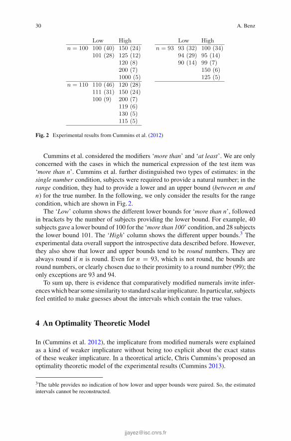
30 A. Benz
Low Highn = 100 100 (40) 150 (24)
101 (28) 125 (12)120 (8)200 (7)1000 (5)
n = 110 110 (46) 120 (28)111 (31) 150 (24)100 (9) 200 (7)
119 (6)130 (5)115 (5)
Low Highn = 93 93 (32) 100 (34)
94 (29) 95 (14)90 (14) 99 (7)
150 (6)125 (5)
Fig. 2 Experimental results from Cummins et al. (2012)
Cummins et al. considered the modifiers ‘more than’ and ‘at least’. We are onlyconcerned with the cases in which the numerical expression of the test item was‘more than n’. Cummins et al. further distinguished two types of estimates: in thesingle number condition, subjects were required to provide a natural number; in therange condition, they had to provide a lower and an upper bound (between m andn) for the true number. In the following, we only consider the results for the rangecondition, which are shown in Fig. 2.
The ‘Low’ column shows the different lower bounds for ‘more than n’, followedin brackets by the number of subjects providing the lower bound. For example, 40subjects gave a lower bound of 100 for the ‘more than 100’ condition, and 28 subjectsthe lower bound 101. The ‘High’ column shows the different upper bounds.3 Theexperimental data overall support the introspective data described before. However,they also show that lower and upper bounds tend to be round numbers. They arealways round if n is round. Even for n = 93, which is not round, the bounds areround numbers, or clearly chosen due to their proximity to a round number (99); theonly exceptions are 93 and 94.
To sum up, there is evidence that comparatively modified numerals invite infer-enceswhichbear some similarity to standard scalar implicature. In particular, subjectsfeel entitled to make guesses about the intervals which contain the true values.
4 An Optimality Theoretic Model
In (Cummins et al. 2012), the implicature from modified numerals were explainedas a kind of weaker implicature without being too explicit about the exact statusof these weaker implicature. In a theoretical article, Chris Cummins’s proposed anoptimality theoretic model of the experimental results (Cummins 2013).
3The table provides no indication of how lower and upper bounds were paired. So, the estimatedintervals cannot be reconstructed.

Causal Bayesian Networks, Signalling Games … 31
Optimality Theory (OT) was introduced to phonology in the early 1990s (Princeand Smolensky 1993). It describes grammar as a symbolic system in which sur-face forms are considered solutions to a constraint optimisation problem. The con-straints are violable and hierarchically ranked according to their strength such thatthe stronger constraints strictly dominate the weaker constraints. In a productionmodel, the linguistic surface forms are the optimal output forms for an underly-ing input form. Cummins (2013) proposes an OT production model in which theconstraints are special instances of Gricean maxims. The output forms are themodified numerals ‘more than n’, for example, ‘more than 50’, ‘more than 60’,‘more than 70’, etc. The input from which these surface forms are generated are thespeaker’s information states.
In the experiments of (Cummins et al. 2012), subjects first read a text containingthemodified numeral ‘more than n’, and had then to estimate lower and upper boundsfor the true number. For the experimental item shown in Fig. 1, the text may havesaid, for example, that ‘More than 100 people attended the public meeting about thenew highway construction project.’ Cummins’s OT model is a model of the authorproducing the text. It tells us for which speaker information states the text is anoptimal output. The assumption is that, as the OT model is common knowledge, thesubjects can use this knowledge for inferring the underlying information state, andthereby for inferring the lower and upper bounds.
The optimal output for an information state is calculated with the help of a tableauas that shown in (9). The left upper corner of (9) shows the information state ofknowing that between 101 and 109 people came to the meeting. In the column underthe information state all possible outputs are listed. Cummins assumes that onlymodified numerals enter the competition. The constraints are listed in the top row.4
First, there is the Quality constraint, which asks the speaker to say only what hebelieves to be true. This constraint is assumed never to be violated. It is thereforealways to be ranked highest. Next come the Quantity constraint, which asks thespeaker to choose the most informative output, and the Salience constraint, whichasks the speaker to choose round numbers. It is assumed that different speakers cancome with different rankings of Quantity and Salience. Hence, from the hearerperspective, these constraints can be arbitrarily ordered. In (9), this is indicated bythe dashed vertical line between the last two columns.
(9)
101–109 Quality Quantity Salience
more than 110 ∗! ∗∗☞ more than 100
more than 90 ∗! ∗∗more than 80 ∗!∗ ∗
4The full model also contains a constraint preferring the re-use of previously mentioned (primed)numerals. For the special problem of implicatures from ‘more than n’ for round numerals n, thisconstraint can be left out of consideration. It becomes relevant for non–round numerals, as in ‘morethan 93’. We also changed constraint naming: Cummins’s tableaux do not include (Quality), and wecall the quantity maxim by its conventional name of Quantity instead of Informativity, whichCummins chose.

32 A. Benz
As the speaker believes that the true number of people coming to the meeting doesnot exceed 109, it would violate the Quality constraint to say that ‘More than 110came’. This is indicated by the ∗ in the column below Quality. All other numeralssatisfy the constraint. The numerals 90 and 80 are less informative than 100. Thisis indicated by the ∗ in the column below Quantity. The violation is stronger for80 than for 90, hence, 80 receives two stars and 90 only one star. The Salienceconstraint measures the roundness of the chosen numeral. In the given example, 100is rounder than 80, and 80 is rounder than 90 and 110. The violation of Salience,shown in the last column, grows stronger with decreasing roundness.
An output F wins over another output G, if the first constraint for which theydiffer is violated more strongly by G than by F . ‘More than 100’ is the only outputwhich satisfies all constraints. It therefore wins the competition. The ‘!’ in other rowsmarks the first violationwhichmakes the corresponding output loose the competitionwith the winning form.
Cummins’s measure of roundedness is based on the corpus studies of Jansen andPollmann (2001). As an indicator of the degree of roundness Jansen and Pollmannconsidered the frequencies of numerals in approximation contexts created by, forexample, Dutch ‘ongeveer’, German ‘etwa’, French ‘environ’, and English ‘about’.The more frequent a numeral is in such contexts, the rounder it is assumed to be.
Cummins’s OT model makes predictions about which numerals n are optimal in‘more than n’ contexts. He provides an explanation for why round numerals allow fora larger range of upper bounds. He also claims that his model explains the ignoranceimplicature from ‘more than n’ to the speaker believes it possible that n+1 (♦n+1).
Thewider range of upper bounds for round numerals is explained as a consequenceof the free ranking of the Quantity and Salience constraints. For example, if thespeaker knows that the true number of people attending some event lies in the openinterval (150, 200), then, assuming that 100 is rounder than 150, it follows that aspeaker ranking Salience over Quantity will prefer the less precise ‘more than100’ over ‘more than 150’. If, in contrast, the speaker knows that the true numberlies in some interval above 100, for example in the interval (110, 120), then there isno constraint ranking which could make the choice of ‘more than 90’ optimal. Thisrestricts the allowed range for the true number to (90, 100) for ‘more than 90’, andallows a wide range for ‘more than 100’. However, if the belief interval is (150, 200)and Salience is ranked higher than Quantity, then the model not only predictsthat ‘more than 100’ wins over ‘more than 150’, but also that ‘more than 10’ winsover ‘more than 100’, as 10 is rounder than 100.5 Hence, the speaker should choose‘more than 10’. The model also predicts, as there is no higher number rounder than100, that ‘more than 100’ wins over all alternatives ‘more than n’ for numbers ngreater than 100. This is a consequence of the ‘the winner takes it all’ property ofOT models. It entails that the most salient number N , whichever it is, has no upperbound, and all other numbers greater than N can only be used ifQuantity is ranked
5In fact, this depends on which number is considered to be roundest. For example, the frequencygraph in (Jansen and Pollmann 2001, p. 193) shows an even higher peak for 20 than for 10. However,pure frequencies may not be the best criteria of roundness.

Causal Bayesian Networks, Signalling Games … 33
over Salience. The model entails, therefore, that the ignorance implicature onlyexist for numbers which are preceded by a more salient number. For the maximallysalient numbers, the implicature from ‘more than N’ to ♦N + 1 does not hold true.If someone who believes the true number to lie in (150, 200) can utter ‘more than100’, then the addressee cannot infer from this utterance that the speaker believes101 to be possible.6
As themodel imposes no restrictions on the possible speaker information states, noinferences about upper bounds can be drawn if Quantity is ranked over Salience.For example, if all intervals (110, Lu) are admissible information states of thespeaker, then from an utterance of ‘more than 110’ no restriction on the upper limitLu can be inferred. It could be arbitrarily large. Cummins obviously assumes somerestrictions on possible information states, but they are not made explicit in hismodel.7
We sympathisewith Cummins’s approach of explaining the observed implicaturesfrom a production model. However, the model has shortcomings which warrant con-sidering alternatives. In particular, it seems necessary to have a model that explicitlydescribes the set of admissible information states. Without it no inferences can bemade about upper bounds.We alsowill drop the optimality theoretic framework.8 Weprefer a representation which describes the communication process and the experi-mental situationmore directly. Aswe aremainly interested in the general architectureof such a representation,we consider only a limited subset of the experimental results.For example, we leave out of consideration non–round numerals, as, for example,93.9 The main question in the next section is how to account for the influence ofroundedness on the estimated difference between lower and upper bounds even if itis assumed that the speaker tries to be as informative as possible, i.e. even if, in OTterms, the speaker ranks Quantity over Salience.
5 A Causal Bayesian Network Model
Our aim is to explain the experimental data shown in Fig. 2 on ‘more than 100’. Themain effort will be to set up a model of the author producing the text appearing in thequestionnaire shown in Fig. 1, for example, the text ‘More than 100 people attendedthe public meeting about the new highway construction project.’
In Fig. 3, a model of the experimental situation which starts with a reported (imag-inary) event and concludes with the test subject’s answer is shown. Each node in this
6This reveals a (minor) inconsistency in Cummins’s argumentation (2013), as he claims that theignorance implicature always holds true.7Excluding examples with anaphoric uses, Cummins always considers information states (n, m) forwhich n and m are adjacent round numbers. Making this aspect explicit would presumably revealthe same application of Jansen and Pollmann’s sequence rule as in our own model.8Itmay also be debated that anOTmodelwith free constraint ranking is still in the spirit of optimalitytheory.9For these numerals, Cummins has also to apply a different model with an additional constraint.

34 A. Benz
N (n, m) ‘more than n’ 〈lb, ub〉World Knowledge Utterance Estimate
forced estimate in experiment
Fig. 3 A model of the Cummins, Sauerland, and Solt experiment (2012)
sequence corresponds to a random variable in a causal Bayesian network. The val-ues of the first variable named World are natural numbers N , those of the thirdvariable named Utterance are sentences containing ‘more than n’ for some naturalnumber n, and the values of the last variable named Estimate are pairs 〈lb, ub〉 oflower and upper bounds for the true number N . In order to complete this model, ithas to be known which values the variable named Knowledge can take, and it hasto be known what the conditional probabilities of the various values are.
We will identify the knowledge states with open intervals (n, m) using Jansen andPollmann’s unmodified sequence rule (Jansen andPollmann2001). It is obviously notpossible to determine the conditional probabilities. Fortunately, this is not necessaryas we will see once we know how to define implicature. We address this issue next.
5.1 Implicature in Bayesian Networks
In a Bayesian network, the different random variables carry information about eachother. For our purposes, we can assume that communication is describable by a linearsequence of random variables (Xi , Pi )
ni=1 with conditional probabilities Pi (xi |xi−1)
defined for xi ∈ Xi and xi−1 ∈ Xi−1.With the product probability P(x1, . . . , xn) =P1(x1) × · · · × Pn(xn|xn−1), we can define the probability that the i th variable hasa value in some set X given that the j th variable has a value in Y as follows10:
Pi | j (X |Y ) := P(π−1i (X) ∩ π−1
j (Y ))
P(π−1j (Y ))
with πk(x1, . . . , xn) = xk . (1)
In a linear Bayesian network describing communication, one variable will describethe utterances the speaker produces. Let us assume it is the j th variable, and that theutterance is F . Then we can say that the utterance of F implicates that some othervariable Xi has a value in X iff Pi | j (X |F) = 1.
It follows that, in order to determine implicature, it is only necessary to knowwhich values xi of a variable Xi are consistent with an utterance of F . Hence, itsuffices to know for which xi Pi | j (xi |F) > 0.
10Whenever a probability appears in the denominator, we implicitly assume that it is greater thanzero. If X or Y is a singleton set, for example Y = {y}, the brackets around y are omitted in argumentpositions of probability distributions.

Causal Bayesian Networks, Signalling Games … 35
This definition is justified by Grice’s contention (1989, p. 86) that ‘what is im-plicated is what it [sic!] is required that one assume a speaker to think in order topreserve the assumption that he is observing the Cooperative Principle (and per-haps some conversational maxims as well), …’ The most obvious interpretation isthat what is implicated by an utterance of F is the information that is carried by Fabout values of variables representing the speaker’s beliefs.11
5.2 Knowledge States and the Sequence Rule
All estimated lower and upper bounds shown in Fig. 2 are round numbers, or differonly by a value of one froma roundnumber.Aswehave seen, the speaker’s preferencefor round numbers is also a key element of Cummins’s OT model. In the Bayesiannetwork in Fig. 3, the (imaginary) speaker’s first task is to estimate the true numberof people taking part in some event. We assume with Cummins’s that this estimateis some interval. More specifically, we assume that it is an open interval (n, m) withat least two elements defined by two round numbers n and m. To further restrictthe admissible pairs of numbers n, m, we make use of the corpus study by Jansenand Pollmann (2001) who found that pairs of numbers n, m in the approximativeconstruction ‘about n or m’ follow the following rule:
(10) Sequence rule:12 For context ‘about n or m’, the numbers n, m follow eachother directly in a sequence:
Lk,l = {i (k × 10l) ∈ N | i ∈ N} with k = 1, 2, 1/2, 1/4, and l ≥ 0. (2)
The following list in (11) shows all sequences which are relevant to us.
(11)
L1,0 = 1, 2, 3, 4, 5, . . .L2,0 = 2, 4, 6, 8, 10, . . .L1/2,1 = 5, 10, 15, 20, . . .L1,1 = 10, 20, 30, 40, 50,. . .
L2,1 = 20, 40, 60, 80, . . .L1/4,2 = 25, 50, 75, . . .L1/2,2 = 50, 100, 150, 200, . . .L1,2 = 100, 200, 300, 400, 500,. . .
11This definition deviates from common usage in so far as it includes literal meaning in implicatedmeaning, whereas what is implicated is generally understood to be the meaning that is commu-nicated but not literally expressed. For simplicity, we use this inclusive definition, which can beeasily modified to bring it more in line with common usage. We may mention that Grice’s originalcharacterisation of conversational implicatures also does not exclude literal meaning (Grice 1989,p. 30f).12This is the unmodified sequence rule. Jannsen and Pollmann (2001) see no justification for theinclusion of k = 1/4. However, we can ignore this modification for our purposes. For k = 1/4,l must be greater than 1 to make sure that all elements of L1/4,l are natural.

36 A. Benz
Let us write (n, m) � Lk,l if n and m are consecutive numbers in sequence Lk,l . Weassume that (n, m) is a possible information state if n andm are consecutive numbersin some sequence Lk,l . In addition, we assume that the speaker’s estimate is correct,i.e. that the true number N is an element of (n, m). Translated into conditionalprobabilities P((n, m)|N ), this means:
P((n, m)|N ) > 0 iff ∃k∃l > 0 : (n, m) � Lk,l ∧ N ∈ (n, m). (3)
As mentioned before, it suffices for implicature calculation to know whenprobabilities are greater zero. In order to rule out intervals with one or zero ele-ments, we assume that l > 0.
5.3 Speaker’s Strategy and Experimental Data
The last parameter to be fixed for the model in Fig. 3 is the probability with whichthe speaker chooses ‘more than n’ given that his knowledge state is (n′, m′). Ingame theoretic terminology, this conditional probability can be called the speaker’sstrategy. We make the assumption that the speaker can only produce Fn = ‘morethan n’ if n′ = n:
S(Fn|(n′, m′)) > 0 iff n = n′. (4)
The situations represented by condition (4) correspond to those situations in whichQuantity is ranked higher than Salience in Cummins’s optimality theoreticmodel.As we have seen, for these cases, the optimality theoretic model cannot make pre-dictions about upper bounds. In Sect. 5.4, we will shortly discuss cases in which thespeaker could have beenmore informative; for example, cases inwhich he could havebeen more informative because he knew that exactly 93 people came to an event, butnevertheless chose the less informative lower bound ‘more than 90’.
This completes the set-up of our model. The probabilities with which the testsubjects choose their estimates and the nature of the estimates are provided by theexperimental data.
The table in (12) lists the belief intervals which have probability greater zero giventhat the speaker uttered Fn for the numbers n = 80, 90, 100. To each interval, thesequence to which the interval belongs is added. More precisely, if F is the nameof the random variable representing utterances, and Θ the random variable for thespeaker’s belief, then the intervals (n, m) listed in table (12) are those for whichPΘ|F ((n′, m′)|Fn) > 0.

Causal Bayesian Networks, Signalling Games … 37
(12) Fn belief intervals
‘more than 80’ L1/2,1 (80, 85) L1,1 (80, 90)L2,1 (80, 100)
‘more than 90’ L1/2,1 (90, 95) L1,1 (90, 100)
‘more than 100’ L1/2,1 (100, 105) L1,1 (100, 110)L2,1 (100, 120) L1/4,2 (100, 125)L1/2,2 (100, 150) L1,2 (100, 200)
Given our definition of implicature, this table says that an utterance of ‘more than80’ implicates that the speaker believes that the true number is an element of (80, 85),(80, 90), or (80, 100). Likewise, an utterance of ‘more than 100’ implicates that thespeaker estimates the true number to lie in one of the intervals with lower bound100 and upper bounds 105, 110, 120, 125, 150, and 200. Accordingly, followingfrom the assumption that the speaker’s beliefs are true, an utterance of ‘more than100’ implicates that the true number lies in the interval (100, 200), and an utteranceof ‘more than 80’ that it lies in the interval (80, 100). The model accounts for thedifferent ranges of estimated intervalswithout having to rank the preference for roundnumbers over the preference for information. Equation (4) entails that the speakerchooses the most informative version of ‘more than n’. The model also accounts forthe ignorance implicature ‘more than n’ implicating possibly n + 1.
It is difficult to say how test subjects construed the task in the questionnaire. Theywere not explicitly asked for implicatures, only for estimated lower and upper limitsof the true number N . It is plausible to assume that they provided probable and safelimits within which the speaker’s belief intervals lie. The experimental results for‘more than 100’ are repeated in (13). We find a good match between the predictedset of possible upper bounds and elicited upper bounds. The only predicted upperbounds which cannot be found in the experimental data are 105 and 110, and theonly upper bound not predicted is 1000.
(13) Low Highn = 100 100 (40) 150 (24)
101 (28) 125 (12)120 (8)200 (7)1000 (5)
A plausible reason for the missing 105 and 110 is that the resulting intervals wouldbe too small. As test subjects had no information about speakers, the belief intervals(100, 105) and (100, 110)would have been too unlikely to be the only speaker types.On the other side, the estimated upper bound of 1000 may be the result of a specialsafety strategy of test subjects.13
13In the cognitive literature it is also argued that the distances on themental number line are rescaledaccording to some logarithmic rule (Dehaene 2011). This may have an effect on choosing upperbounds which is not accounted for in our model but may explain why some people estimate the truenumber to lie between ‘100 and 1000.’

38 A. Benz
5.4 Extensions of the Basic Model
In the basic model we only considered the case in which the assumed speaker of thetest sentence believes that the true number N can lie anywhere in an open interval(n, m). When he produces an utterance with ‘more than’, then he always chooses nas the lower bound. This was encoded in Eq. (4). In this section, we consider otherstrategies which may lead to utterances containing ‘more than n’. The reasoning isadmittedly even more speculative than in the previous sections. The aim is to showthat the constraints over possible estimates for the interval containing the true numberN that may be produced by the test subjects remain valid also when considering otherspeaker strategies which might have produced the test sentences. A second aim isto show how the sequence rule might be used to capture a variety of other reasonsleading to utterances with numerals modified by ‘more than’.
We first consider the following possibility: If the speaker says that ‘More than 90people attended the public meeting about the new highway construction project’, it isconceivable that he knows that exactly 93 people attended but chose the round number90 as lower bound for ‘more than n’. In Cummins’smodel one has to assume here thatSalience outranksQuantity. If the speaker knows that exactly N people attended,the dominance of Salience overQuantitymeans that the speaker must choose theroundest number n smaller or equal to N . However, as we have seen, the restrictionto the roundest number smaller than N seems to be too strong a requirement. Wewill now show how a prediction about possible lower bounds n can be derived fromthe sequence rule. It can be assumed that the different sequences Lk,l resulting fromdifferent choices of numbers k = 1, 2, 1/2, 1/4 and l ∈ N represent different levels ofprecision with which the speaker wants to describe the true situation. In the followingmodel, it is assumed that the speaker, who knows that exactly N people attended,first chooses a level of precision Lk,l with which he wants to describe the situation,and then the largest number n in Lk,l which is smaller than N as a lower boundfor ‘more than n’. The following constraint, which modifies the conditions statedin Eqs. (3) and (4), captures this idea. It says that Fn = ‘more than n’ is a possibleutterance if there is an interval (n, m) of adjacent numbers in some sequence Lkl
which contains N :
S(Fn|N ) > 0 iff ∃k∃l > 0 ∃m > n : (n, m) � Lk,l ∧ N ∈ (n, m). (5)
For N = 93, this rule predicts that the speaker can produce the following sentences:
(14) (a) More than 90 people attended. ((n, m) = (90, 95), (90, 100))(b) More than 80 people attended. ((n, m) = (80, 100))(c) More than 75 people attended. ((n, m) = (75, 100))(d) More than 50 people attended. ((n, m) = (50, 100))
These are all possibilities. Numbers like n = 20 or n = 10 are ruled out becausethere is no sequence Lk,l for which there exist intervals (20, m) or (10, m) that wouldcontain 93 as an element. What is important with respect to the experimental data of

Causal Bayesian Networks, Signalling Games … 39
Cummins et al. (2012) is that the strategy defined in (5) does not introduce expectedintervals (n, m) different from the intervals introduced by the basic rule in (4): If theaddressee hears that e.g. ‘more than 80 people attended’, then she can infer that thetrue number is an element of (80, 100). So, even when the addressee does not knowwhether the speaker’s information state is an interval or an exact number, she shouldarrive at the same estimates.
Let us consider one further scenario. It is conceivable that the speaker countedthe people attending the meeting and stopped counting at, say, 91. He may be certainthat at least twomore attended, and, maybe, up to a hundred. When asked, howmanywere there, he may well answer ‘more than 90’. Also for such a scenario we canderive a plausible model from Jansen and Pollmann’s sequence rule. In our example,the speaker knows that at least 93 attended. So let N be any number, not necessarilyround, for which the speaker verified by counting that at least N attended. Thenthe following strategy produces plausible ‘more than n’ utterances with round lowerbounds n:
S(Fn|(N , m)) > 0 iff ∃k∃l > 0 : (n, m) � Lk,l ∧ N ∈ (n, m). (6)
The predicted intervals for N = 93 are the same as in (14). This also means that thehearer, when confronted with a ‘more than n’ message, has no reason to change herestimates for the interval containing the true number.
As mentioned before, the modifications presented in this section are increas-ingly speculative. However, they demonstrate how the model can be extended tocover more scenarios in which the speaker can produce a comparatively modifiednumeral. In terms of linguistic depth, the achievements may seem modest. Evenwith the extensions presented, the model does not account for vague interpreta-tions of unmodified numerals, as, for example, in ‘A hundred people came to thetalk’, which can mean that about 100 people came. It also does not account for anutterance of ‘more than 93’. For these examples, the model has to take into accountadditional parameters, e.g. previouslymentionednumerals, and contextually requiredprecision. This leads to nontrivial extensions, which we leave to future research.
Before we end this section, we provide an overview of how roundness can influ-ence the experimental results in the setting of Cummins et al. (2012). In our basicmodel, roundness entered the definition of conditional probabilities of belief inter-vals. However, roundness can also influence the choice of utterances and the intervalestimation by the test subject. These possibilities are shown in Fig. 4.
N (n, m) F (lb, ub)World Knowledge Utterance Estimate
R
Fig. 4 Influence of roundness R on probabilities

40 A. Benz
If roundness determines the formation of belief intervals, then the (imaginary)speaker of the ‘more than n’ sentence is restricted to belief states (n, m) with roundneighbours in a Jansen and Pollmann sequence, as assumed in our basic model. Ifroundness enters the choice of utterance, then the speaker may produce ‘more than100’ although he knows that there are more than 110. This is the case we haveconsidered in this section. There is also the possibility that roundness enters thechoice of the test subject’s estimate of the interval containing the true number. Thiscase we have not considered so far. For example, the test subject may estimate thatthe true number is between 103 and 150, but when asked for lower and upper bounds,she may respond between 100 and 150, simply because (100, 150) is a particularlysalient interval. However, to disentangle how roundness exactly influences whichmodule in Fig. 4 needs further experimental investigations.
6 Implicature in Which Sense?
In this section we consider the question what type of implicature are inferences from‘more than n’ to upper bounds for the true n. Krifka (1999) maintained that ‘morethan n’ does not generate implicatures. Cummins et al. (2012) considered ‘more thann’ implicature to be weak implicatures compared to standard scalar implicatures.Cummins (2013) explained them as inferences about the speaker’s beliefs which areinferred from an optimality theoretic production model. In this model, there seemsto be no principled difference between implicature from ‘more than n’ and thosefrom unmodified numerals, for example, from ‘John has three children’ to John hasexactly three children.
We quoted before a passage from Grice which says that an implicature is whatis required that one assume a speaker to think in order to preserve the assumptionthat he is following the conversational maxims. This suggests that an implicature isan inference about some belief of the speaker. However, in (Grice 1989, Chap. 14),Grice defined communicated meaning as meaning that the speaker intended to com-municate. Thismakes an implicature an inference about intentions, and not just aboutsome belief he happens to entertain. Accordingly, we can distinguish between twotypes of implicature:
(15) (a) (Grice–B): A belief of the speaker. (Logic of Conversation, Grice 1989,Chap. 2)
(b) (Grice–I): The part of the intendedmeaningwhich is not literally expressed.(Meaning, Grice 1989, Chap. 14)
These implicature can be distinguished in a causal model if distinct nodes for beliefsand intentions are introduced, as shown in Fig. 5.
The standard examples of scalar implicature in (16) are clearly part of what hasbeen communicated. Hence, they constitute Grice–I implicature.

Causal Bayesian Networks, Signalling Games … 41
Fig. 5 Grice–B and Grice–Iimplicature W Θ L F
World Knowledge Message Utterance
Grice–I
Grice–B
(16) (a) Some of the students failed the exam. +> not all failed.(b) John has three children. +> He has not more than three.
However, the implicatures about upper bounds in (7), repeated here as (17), arenormally not part of what the speaker intended to communicate. In this sense theyare weaker implicature as Cummins et al. (2012) maintained.
(17) (a) More than 80 people got married today. +> between 80 and 100(b) More than 90 people got married today. +> between 90 and 100(c) More than 100 people got married today. +> between 100 and 200
This becomes also apparent from the causal model we considered in the previoussection. Implicature from ‘more than n’ were there considered inferences about thespeaker’s knowledge.
This also reconciles Krifka’s (1999) view that ‘more than n’ does not generateimplicature with the experimental results of (Cummins et al. 2012), if one assumesthat Krifka’s claim relates to Grice–I implicature, and not to Grice–B implicature.
7 Conclusion
The main aim of this paper was to show the usefulness of causal networks foranalysing the experimental setting in experiments of the type performed byCumminset al. (2012). Causal networks provide a high level description of communication byshowing the causal dependencies between different modules in language productionand interpretation. They are a very natural framework to use. We have seen how toexplicate the notion of implicature in these networks as inferences from one specialvariable representing utterances to properties of other variables. This provided uswith a general definition, and we could show that, in spite of its abstractness, it helpsto make fine distinctions within the group of quantity implicature.
We have seen that the model provides a good match for upper bounds of ‘morethan 100’. It explains why differences between lower and upper bounds are largerfor round numbers. It also shows that this pattern is consistent with the assumptionthat the speaker tries to be as informative as possible. Hence, the data are consistentwith the ignorance implicature from ‘more than n’ to ‘it is possible that n+1’. Themodel also predicts that ‘more than n’ can only be used with round numbers.
42 A. Benz
We have argued that pragmatic inferences from, for example, ‘more than 100’to ‘less than 200’ are not Grice-I implicatures, hence, that they are not part of thespeaker’s intended message. This makes them different from implicatures triggeredby unmodified numerals, as, for example, by ‘John has three children’ implicatingthat ‘John has exactly three children’. In this sense, we agree with (Krifka 1999; Foxand Hackl 2006) that comparatively modified numerals do not give rise to standardscalar implicatures. The experimental results of (Cummins et al. 2012) seem to bethe consequence of general inferences about the speaker’s probable knowledge state.
References
Benz, A. (2012). Errors in pragmatics. Journal of Logic, Language, and Information, 21, 97–116.Cummins, C. (2011). The interpretation and use of numerically-quantified expressions. Ph.D thesis,University of Cambridge
Cummins, C., Sauerland, U., & Solt, S. (2012). Granularity and scalar implicature in numericalexpressions. Linguistics and Philosophy, 35, 135–169.
Cummins, C. (2013). Modelling implicatures from modified numerals. Lingua, 132, 103–114.Dehaene, S. (2011). The number sense: How the mind creates mathematics. Revised and Updated
Edition. Oxford: Oxford University Press.Fox, D., & Hackl, M. (2006). The universal density of measurement. Linguistics and Philosophy,
29, 537–586.Grice, H. P. (1989). Studies in the way of words. Cambridge: Harvard University Press.Jansen, C. J., & Pollmann, M. M. (2001). On round numbers: pragmatic aspects of numericalexpressions. Journal of Quantitative Linguistics, 8(3), 187–201.
Krifka, M. (1999). At least some determiners aren’t determiners. In K. Turner (Ed.), The se-mantics/pragmatics interface from different points of view. Current research in the seman-tics/pragmatics interface (Vol. 1, pp. 257–292). Oxford: Elsevier.
Levinson, S. C. (1983). Pragmatics. Cambridge: Cambridge University Press.Pearl, J. (2000). Causality: Models, reasoning, and inference. Cambridge: Cambridge UniversityPress.
Prince, A. & Smolensky, P. (1993). Optimality theory: constraint interaction in generative grammar.Technical Report 2, Rutgers University, Centre for Cognitive Science

Measurement-Theoretic Foundationsof Logic for Better Questionsand Answers
Satoru Suzuki
Abstract Groenendijk and Stokhof (Varieties of formal semantics, 143–170, 1984)propose a version of partition-based semantics to analyse questions and answers. Inorder to compare the goodness of answers, they use qualitative orderings amonganswers. Groenendijk and Stokhof’s qualitative method is too coarse-grained toachieve the goal. In order to overcome the limitations, van Rooij (Formal theoriesof information: from Shannon to semantic information theory and general conceptsof information, LNCS, 161–192, 2009) proposes an information-theoretic approachbased on conditional entropy. The aims of this paper are to construct a qualitativeapproach that is as fine-grained as the information-theoretic one, in terms ofmeasure-ment theory on the basis of Domotor (Information and inference, 148–194, 1970),and to propose a new version of complete logic for better questions and answers—Better-Question-and-Answer Logic (BQAL)—the model of the language of whichis based on the qualitative and measurement-theoretic approach.
Keywords (Conditional) entropy · Information theory · Logic for better questionsand answers · Measurement theory · Qualitative conditional entropy relation ·Representation theorem
1 Introduction
Groenendijk and Stokhof (1984) consider the goodness of an answer in terms of thepartition induced by the question.1 AQ is defined as the set of all cells of the partitionQ that are compatible with an answer A:
AQ := {q ∈ Q : q ∩ A �= ∅}.
1 We owe this section to van Rooij (2009).
S. Suzuki (B)Faculty of Arts and Sciences, Komazawa University, 1-23-1 Komazawa, Setagaya-ku,Tokyo 154-8525, Japane-mail: [email protected]
© Springer International Publishing Switzerland 2015H. Zeevat and H.-C. Schmitz (eds.), Bayesian Natural Language Semanticsand Pragmatics, Language, Cognition, and Mind 2,DOI 10.1007/978-3-319-17064-0_3
43

44 S. Suzuki
In order to compare the goodness of answers, they use a qualitative ordering >Q
among answers with relative to Q. Groenendijk and Stokhof propose that when ananswer A is incompatible with more cells of Q than an answer A′, that is, AQ � A′
Q ,A should be counted as a better answer to the question than A′. Van Rooij (2009)gives the following example:
Example 1 The answer A:
(At least) John is sick.
to the question Q:
Who of John and Mary are sick?
is incompatible with 2 of the 4 cells of the partition. The answer A′:If Mary is not sick, then neither is John is.
is incompatible with 1 cell of the partition. According to Groenendijk and Stokhof,A should be a better answer to the question than A′.
What if AQ = A′Q? If A does not give extra irrelevant information, that is, A′ � A, A
is considered to be a better answer than A′. Combining both constraints, Groenendijkand Stokhof define A’s being a better answer to a question Q than A′, in symbols,A >Q A′ as follows:
A >Q A′ iff (i)AQ � A′Q, or
(ii)AQ = A′Q and A′ � A.
Van Rooij gives the following example that Groenendijk and Stokhof’s qualitativemethod cannot deal with, for neither AQ � A′
Q , A′Q � AQ , nor AQ = A′
Q holds:
Example 2 The answer A:
(At least) John and Mary are sick.
to the question Q:
Who of John, Mary and Sue are sick?
is felt to be better than the answer A′:(At least) Sue is sick.2
Groenendijk and Stokhof’s qualitative method is too coarse-grained to deal with thisexample. In order to overcome the limitations, van Rooij proposes an information-theoretic approach based on conditional entropy. He proposes that an answer A isbetter than an answer A′ to a question Q iff the information value IVQ(A) of A withrespect to Q is higher than that of A′, or in case both of them are the same, the
2In Sect. 7, we apply Better-Question-and-Answer Logic (BQAL) to Example2.
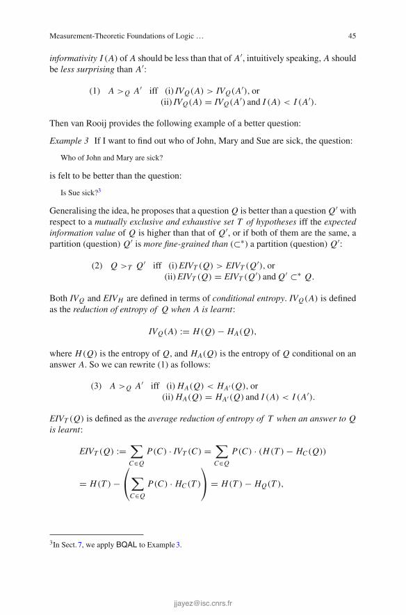
Measurement-Theoretic Foundations of Logic … 45
informativity I (A) of A should be less than that of A′, intuitively speaking, A shouldbe less surprising than A′:
(1) A >Q A′ iff (i) IVQ(A) > IVQ(A′), or(ii) IVQ(A) = IVQ(A′) and I (A) < I (A′).
Then van Rooij provides the following example of a better question:
Example 3 If I want to find out who of John, Mary and Sue are sick, the question:
Who of John and Mary are sick?
is felt to be better than the question:
Is Sue sick?3
Generalising the idea, he proposes that a question Q is better than a question Q′ withrespect to a mutually exclusive and exhaustive set T of hypotheses iff the expectedinformation value of Q is higher than that of Q′, or if both of them are the same, apartition (question) Q′ is more fine-grained than (⊂∗) a partition (question) Q′:
(2) Q >T Q′ iff (i)EIVT (Q) > EIVT (Q′), or(ii)EIVT (Q) = EIVT (Q′) and Q′ ⊂∗ Q.
Both IVQ and EIVH are defined in terms of conditional entropy. IVQ(A) is definedas the reduction of entropy of Q when A is learnt:
IVQ(A) := H(Q) − HA(Q),
where H(Q) is the entropy of Q, and HA(Q) is the entropy of Q conditional on ananswer A. So we can rewrite (1) as follows:
(3) A >Q A′ iff (i) HA(Q) < HA′(Q), or(ii) HA(Q) = HA′(Q) and I (A) < I (A′).
EIVT (Q) is defined as the average reduction of entropy of T when an answer to Qis learnt:
EIVT (Q) :=∑
C∈Q
P(C) · IVT (C) =∑
C∈Q
P(C) · (H(T ) − HC (Q))
= H(T ) −⎛
⎝∑
C∈Q
P(C) · HC (T )
⎞
⎠ = H(T ) − HQ(T ),
3In Sect. 7, we apply BQAL to Example3.
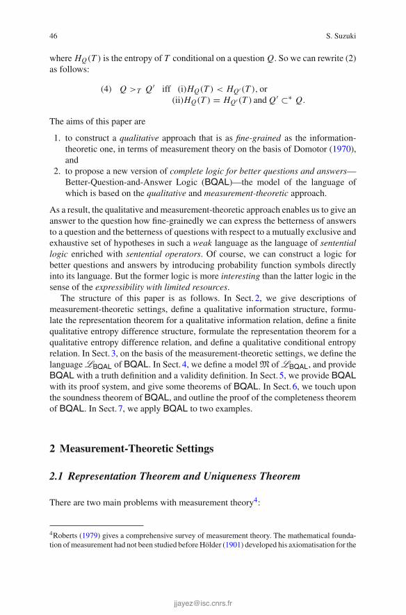
46 S. Suzuki
where HQ(T ) is the entropy of T conditional on a question Q. So we can rewrite (2)as follows:
(4) Q >T Q′ iff (i)HQ(T ) < HQ′(T ), or(ii)HQ(T ) = HQ′(T ) and Q′ ⊂∗ Q.
The aims of this paper are
1. to construct a qualitative approach that is as fine-grained as the information-theoretic one, in terms of measurement theory on the basis of Domotor (1970),and
2. to propose a new version of complete logic for better questions and answers—Better-Question-and-Answer Logic (BQAL)—the model of the language ofwhich is based on the qualitative and measurement-theoretic approach.
As a result, the qualitative and measurement-theoretic approach enables us to give ananswer to the question how fine-grainedly we can express the betterness of answersto a question and the betterness of questions with respect to a mutually exclusive andexhaustive set of hypotheses in such a weak language as the language of sententiallogic enriched with sentential operators. Of course, we can construct a logic forbetter questions and answers by introducing probability function symbols directlyinto its language. But the former logic is more interesting than the latter logic in thesense of the expressibility with limited resources.
The structure of this paper is as follows. In Sect. 2, we give descriptions ofmeasurement-theoretic settings, define a qualitative information structure, formu-late the representation theorem for a qualitative information relation, define a finitequalitative entropy difference structure, formulate the representation theorem for aqualitative entropy difference relation, and define a qualitative conditional entropyrelation. In Sect. 3, on the basis of the measurement-theoretic settings, we define thelanguageLBQAL of BQAL. In Sect. 4, we define a modelM ofLBQAL, and provideBQAL with a truth definition and a validity definition. In Sect. 5, we provide BQALwith its proof system, and give some theorems of BQAL. In Sect. 6, we touch uponthe soundness theorem of BQAL, and outline the proof of the completeness theoremof BQAL. In Sect. 7, we apply BQAL to two examples.
2 Measurement-Theoretic Settings
2.1 Representation Theorem and Uniqueness Theorem
There are two main problems with measurement theory4:
4Roberts (1979) gives a comprehensive survey of measurement theory. The mathematical founda-tion ofmeasurement had not been studied before Hölder (1901) developed his axiomatisation for the

Measurement-Theoretic Foundations of Logic … 47
1. the representation problem—justifying the assignment of numbers to objects,and
2. the uniqueness problem—specifying the transformation up to which this assign-ment is unique.
A solution to the former can be furnished by a representation theorem, which estab-lishes that the specified conditions on a qualitative relational system are (necessaryand) sufficient for the assignment of numbers to objects that represents (preserves) allthe relations in the system. A solution to the latter can be furnished by a uniquenesstheorem, which specifies the transformation up to which this assignment is unique.To construct a model of the language of BQAL, we use two sorts of qualitativeorderings:
1. orderings of information,2. orderings of (conditional) entropy.
2.2 Qualitative Information Structure
Wedefine a qualitative information structure for orderings of information as follows5:
Definition 1 (Qualitative Information Structure) LetW be a non-empty set of pos-sible worlds,F a Boolean algebra of subsets ofW , ⊥⊥ a probabilistic independencerelation on F , and � a relation on F . Then (W ,F ,�,⊥⊥) is said to be a qualita-tive information structure iff the following conditions are satisfied for all variablesrunning over F .
(I1) ∅ ⊥⊥ A,
(I2) If A ⊥⊥ B, then B ⊥⊥ A,
(I3) If A ⊥⊥ B, then BC ⊥⊥ A,
(I4) When B ∩ C = ∅, if A ⊥⊥ B and A ⊥⊥ C, then A ⊥⊥ B ∪ C,
(I5) W ≺ ∅, where A ≺ B := B �� A,
(I6) A � ∅,
(I7) A � B or B � A,
(I8) If A � B and B � C, then A � C,
(I9) If A ⊥⊥ B and A ∩ B = ∅, then A ∼ ∅ or B ∼ ∅,
where A ∼ B := A � B and B � A,
(I10) WhenC ∩ A = ∅ andC ∩ B = ∅, A � B iff A ∪ C � B ∪ C,
(Footnote 4 continued)measurement of mass. Krantz et al. (1971), Suppes et al. (1989) and Luce et al. (1990) are seen asmilestones in the history of measurement theory.5We owe this subsection to Domotor (1970).
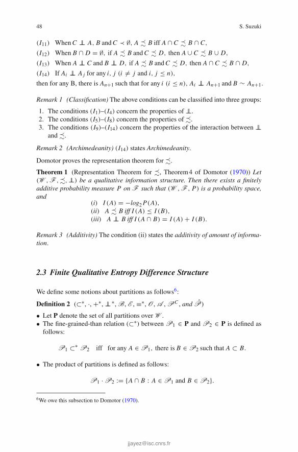
48 S. Suzuki
(I11) WhenC ⊥⊥ A, B andC ≺ ∅, A � B iff A ∩ C � B ∩ C,
(I12) When B ∩ D = ∅, if A � B andC � D, then A ∪ C � B ∪ D,
(I13) When A ⊥⊥ C and B ⊥⊥ D, if A � B andC � D, then A ∩ C � B ∩ D,
(I14) If Ai ⊥⊥ A j for any i, j (i �= j and i, j ≤ n),
then for any B, there is An+1 such that for any i (i ≤ n), Ai ⊥⊥ An+1 and B ∼ An+1.
Remark 1 (Classification) The above conditions can be classified into three groups:
1. The conditions (I1)–(I4) concern the properties of ⊥⊥.2. The conditions (I5)–(I8) concern the properties of �.3. The conditions (I9)–(I14) concern the properties of the interaction between ⊥⊥
and �.
Remark 2 (Archimedeanity) (I14) states Archimedeanity.
Domotor proves the representation theorem for �.
Theorem 1 (Representation Theorem for �, Theorem4 of Domotor (1970)) Let(W ,F ,�,⊥⊥) be a qualitative information structure. Then there exists a finitelyadditive probability measure P on F such that (W ,F , P) is a probability space,and
(i) I (A) = −log2P(A),
(ii) A � B iff I (A) ≤ I (B),
(iii) A ⊥⊥ B iff I (A ∩ B) = I (A) + I (B).
Remark 3 (Additivity) The condition (ii) states the additivity of amount of informa-tion.
2.3 Finite Qualitative Entropy Difference Structure
We define some notions about partitions as follows6:
Definition 2 (⊂∗, ·, +∗, ⊥⊥∗,B, E , ≡∗, O , A ,PC , and P)
• Let P denote the set of all partitions over W .• The fine-grained-than relation (⊂∗) between P1 ∈ P and P2 ∈ P is defined asfollows:
P1 ⊂∗ P2 iff for any A ∈ P1, there is B ∈ P2 such that A ⊂ B.
• The product of partitions is defined as follows:
P1 · P2 := {A ∩ B : A ∈ P1 and B ∈ P2}.
6We owe this subsection to Domotor (1970).

Measurement-Theoretic Foundations of Logic … 49
• The sum of partitions is defined as follows:
P1 +∗ P2 :=∏
P1⊂∗P,P2⊂∗P{P},
where∏
denotes the generalisation of the operation.• P1 ⊥⊥∗P2 iff, for any A, B ∈ F , if A ∈ P1 and B ∈ P2, then A ⊥⊥ B.• If A ∈ F , the partition {A, AC } is called a Bernoulli partition. The variablesB,B1,B2, . . . will run over Bernoulli partitions.
• A partition P is called equiprobable iff, for any A, B ∈ F , if A, B ∈ P , thenA ∼ B. The variable for equiprobable partitions will be E ,E1,E2, . . ..
• We call two partitions equivalent modulo ∼, in symbol,
P1 ≡∗ P2, iffP2 = [B1|A1]([B2|A2](. . . ([Bn|An]P1) . . .)),
where [Bi |Ai ]P is the partition that is the result of replacing Bi inP by Ai , and,for any i ≤ n, (Ai ∼ Bi and Bi ∈ P1).
• O := {∅,W }.• A := {{w} : w ∈ W }.• PC :=
∏
P ·Q=A,P⊥⊥∗Q{Q}.
• Let (P = P1 � P2) := (P = P1 · P2 and P1 ⊥⊥∗P2 and P1,P2 �≡∗ O).Let B := {P ∈ P : ¬∃P1,P2(P = P1 � P2)}. Moreover, let D enumerateB, so that B = {Di }i≤k . Then we define
P := (d1, d2, . . . , dk),
where, ifP = Di (1 ≤ i ≤ k), then di = 1, and, for any j ( j �= i and 1 ≤ j ≤ k),d j = 0; otherwise P = Q1 + Q2 for some Q1,Q2 ∈ P. O := (0, 0, . . . , 0).
Remark 4 (Vector Space) P ∈ V (B), where B is the basis of the k dimensionalvector space V (B).
By means of Definition2, we define a finite qualitative entropy difference structurefor ordering of conditional entropy as follows:
Definition 3 (Finite Qualitative Entropy Difference Structure) Let W be a non-empty finite set of possible worlds, P an algebra of finite partitions over W , ⊥⊥ ∗a probabilistic independence relation on P, and �∗ a relation on P × P. Then thequadruple (W , P,�∗,⊥⊥∗) is said to be a finite qualitative entropy difference struc-ture iff the following conditions are satisfied for all variables running over P:

50 S. Suzuki
(D1) IfP1 ⊂∗ P2, then (P2,P) �∗ (P1,P),
(D2) If (B,O) ∼∗ (E ,O), then (O,P) ≺∗ (B,P),
whereP1 ∼∗ P2 := (P1 �∗ P2 andP2 �∗ P1), andP1 ≺∗ P2 := P2 ��∗P2,
(D3) (P1,P2) �∗ (Q1,Q2) or (Q1,Q2) �∗ (P1,P2),
(D4) If (P1,P2) �∗ (Q1,Q2), then (Q2,Q1) �∗ (P2,P1),
(D5) If, for i (i < n), (Pi ,Qi ) �∗ (Ri ,Ti ), then (Rn,Tn) �∗ (Pn,Qn),
when∑
i≤n
Pi =∑
i≤n
Ri and∑
i≤n
Qi =∑
i≤n
Ti ,
(D6) If |P| = |E |, then (P,O) �∗ (E ,O),where | | denotes the cardinalityof a partition,(D7) (P ∪ {∅},O) ≺∗ (P,O).
Remark 5 (Dependence) The qualitative entropy difference relation �∗ depends ontwo factors: the underlying algebra of partitionsP and the probabilistic independencerelation ⊥⊥∗ defined on this algebra. ⊥⊥∗ is used in the definition of Pi in (D5).
Domotor proves the representation theorem for �∗.
Theorem 2 (Representation Theorem for �∗, Theorem8 of Domotor (1970))(W , P,�∗,⊥⊥∗) is a finite qualitative entropy difference structure iff there existsa function H : P → IR satisfying the following conditions for all variables runningover P:
(i) H(P) = −∑
A∈PP(A) · log2 P(A),
(ii) H(P1|P2) = −∑
A∈P1
∑
B∈P2
P(A ∩ B) · log2 P(A|B),
(iii) (P1,P2) �∗ (Q1,Q2) iff H(P1) − H(P2) ≤ H(Q1) − H(Q2),
(iv) IfP1 ⊥⊥∗P2, then H(P1 · P2) = H(P1) + H(P2),
(v) IfP1 ⊂∗ P2, then H(P2) ≤ H(P1),
(vi) H(O) = 0,(vii) If (B,O) ∼∗ (E ,O), then H(B) = 1,(viii) H(P1|P2) = H(P1 · P2) − H(P2).
We define a qualitative conditional entropy relation P1|P2 �∗ Q1|Q2 by a quali-tative entropy difference relation as follows:
Definition 4 (Qualitative Conditional Entropy Relation)
P1|P2 �∗ Q1|Q2 := (P1 · P2,P2) �∗ (Q1 · Q2,Q2).

Measurement-Theoretic Foundations of Logic … 51
3 Language of BQAL
On the basis of the measurement-theoretic settings of Sect. 2, we can provide Better-Question-and-Answer Logic (BQAL) with its language. We define the betternessof answers to a question and the betterness of questions with respect to a mutuallyexclusive and exhaustive set of hypotheses in terms of qualitative information andqualitative entropy difference. Moreover, the language ofBQAL includes a necessityoperator �. The aim of introducing � is as follows. Let W be a non-empty set ofpossible worlds. Then, in each w ∈ W , there may be different universes,Ww, relativeto w. For not every w ∈ W might be able to be taken into consideration. To make thispoint explicit, we introduce an accessibility relation R onW . By means of R, we candefineWw as {w′ ∈ W : R(w, w′)}. R(w, w′) is interpreted tomean that, inw,w′ ∈ Wcan be imagined as an alternative to w. We need � to verbalise the behaviour of Rin BQAL. So we define the language LBQAL of better-question-and-answer logicBQAL as follows:
Definition 5 (Language) LetS denote a set of sentential variables, � and � unarysentential operators, � and ⇓ binary sentential operators, and �∗ a quaternary sen-tential operator. The language LBQAL of BQAL is given by the following BNFgrammar:
ϕ ::= s | � | ¬ϕ | ϕ ∧ ϕ
α ::= ϕ | ϕ ⇓ ϕ |ϕ � ϕ | ¬α | α ∧ α | �α
Φ ::= ¬((
¬n∧
i=1
(¬ϕi )
)∧ ¬�
)∧ ¬
(� ∧
n∧i=1
(¬ϕi )
)
∧ ∧1≤i �= j≤n
(¬((ϕi ∧ ϕ j ) ∧ �) ∧ ¬(¬� ∧ ¬(ϕi ∧ ϕ j )))
A ::= ϕ | α | (Φ,Φ) �∗ (Φ,Φ) | �1≤i≤n Φi | ¬A | A ∧ A
such that s ∈ S .
• ⊥,∨,→,↔, and ♦ are introduced by the standard definitions.• ϕ ⇓ ψ is interpreted to mean that ϕ is probabilistically independent from ψ .• �α is interpreted to mean that necessarily α.• ϕ � ψ is intuitively interpreted to mean that the answer that ϕ is less surprisingthan or as surprising as the answer that ψ .
• (Φ,Ψ ) �∗ (X, T ) is intuitively interpreted to mean that the difference in uncer-tainty between the question as to whether Φ and the question as to whether Ψ
is felt to be less than or as little as the difference in uncertainty between thequestion as to whether X and the question as to whether T.
• �1≤i≤nΦi denotes the symmetric difference of Φ1, . . . , Φn .• �,≈, �∗ and ≈∗ are defined as follows:
– ϕ � ψ := ¬(ψ � ϕ).– ϕ ≈ ψ := (ϕ � ψ) ∧ (ψ � ϕ).

52 S. Suzuki
– (Φ,Ψ ) �∗ (X, T ) := ¬((X, T ) �∗ (Φ,Ψ )).– (Φ,Ψ ) ≈∗ (X, T ) := ((Φ,Ψ ) �∗ (X, T )) ∧ ((X, T ) �∗ (Φ,Ψ )).
• �X and �∗X are defined as follows:
−ϕ �X ψ :=((Φ ∧ X, T ) �∗ (Ψ ∧ X, T ))
∨(((Φ ∧ X, T ) ≈∗ (Ψ ∧ X, T )) ∧ (ϕ � ψ)),where
⎧⎪⎨
⎪⎩X :=
( m∨
i=1
χi ↔ �)
∧∧
1≤i �= j≤m
((χi ∧ χ j ) ↔ ⊥),
T := ((τ1 ↔ ⊥) ∧ (τ2 ↔ �)) ∨ ((τ1 ↔ �) ∧ (τ2 ↔ ⊥)).
−Φ �∗X Ψ :=
((X ∧ Φ,Φ) �∗ (X ∧ Ψ,Ψ ))
∨⎛
⎝((X ∧ Φ,Φ) ≈∗ (X ∧ Ψ,Ψ )) ∧m∧
i=1
l∨
j=1
(ψi → ϕ j )
⎞
⎠ ,where
⎧⎪⎪⎪⎪⎪⎪⎪⎪⎪⎪⎨
⎪⎪⎪⎪⎪⎪⎪⎪⎪⎪⎩
Φ :=( l∨
i=1
ϕi ↔ �)
∧∧
1≤i �= j≤l
((ϕi ∧ ϕ j ) ↔ ⊥),
Ψ :=( m∨
i=1
ψi ↔ �)
∧∧
1≤i �= j≤m
((ψi ∧ ψ j ) ↔ ⊥),
X :=( n∨
i=1
χi ↔ �)
∧∧
1≤i �= j≤n
((χi ∧ χ j ) ↔ ⊥).
• ϕ �X ψ is intuitively interpreted to mean that the answer that ϕ is better than theanswer that ψ to the question as to whether/which/who · · · X .
• Φ �∗X Ψ is intuitively interpreted to mean that the question as to whether/which/
who · · · Φ isbetter than thequestion as towhether/which/who · · · Ψ on amutuallyexclusive and exhaustive set of hypotheses as to whether/which · · · X .
The set of all well-formed formulae of LBQAL will be denoted by ΦLBQAL.
4 Semantics of BQAL
4.1 Model of LBQAL
We define a structured model M of LBQAL as follows:

Measurement-Theoretic Foundations of Logic … 53
Definition 6 (Model) M is a quintuple (W , R, V, ρ, ρ∗) in which
• W is a non-empty (not necessarily finite) set of possible worlds,• R is a binary accessibility relation on W ,• V is a truth assignment to each s ∈ S for each w ∈ W , and• ρ is a qualitative information structure assignment that assigns to each w ∈ Wa qualitative information structure (Ww,Fw,�w,⊥⊥ w) in which
– Ww := {w′ ∈ W : R(w, w′)} that is not necessarily finite,– Fw is a Boolean algebra of subsets of Ww with ∅ as zero element and Ww asunit element, and
– �w is a relation on Fw that satisfies all of the conditions (I1)–(I14) of Defini-tion1.
– ⊥⊥ w is probabilistic independence relation onFw.
• ρ∗ is a qualitative entropy difference structure assignment that assigns to eachw ∈ W a qualitative entropy difference structure (Ww, Pw,�∗,⊥⊥∗) in which
– P an algebra of partitions over Ww, and– �∗
w is a relation on Pw × Pw that satisfies all of the conditions (D1)–(D7) ofDefinition 3.
– ⊥⊥ ∗w is probabilistic independence relation on Pw.
4.2 Truth and Validity
We provide BQAL with the following truth definition relative to M and then definevalidity as follows:
Definition 7 (Truth and Validity) The notion of ϕ ∈ ΦLBQAL being true at w ∈ WinM, in symbols (M, w) |=LBQAL ϕ is inductively defined as follows:
• (M, w) |=LBQAL s iff V (w)(s) = true,• (M, w) |=LBQAL �,• (M, w) |=LBQAL ϕ ∧ ψ iff (M, w) |=LBQAL ϕ and (M, w) |=LBQAL ψ ,• (M, w) |=LBQAL ¬ϕ iff (M, w) �|=LBQAL ϕ,• (M, w) |=LBQAL ϕ ⇓ ψ iff [[ϕ]]Mw ⊥⊥ w[[ψ]]Mw ,
• (M, w) |=LBQAL ϕ � ψ iff [[ϕ]]Mw �w [[ψ]]Mw , in which [[ϕ]]Mw := {w′ ∈ W :R(w, w′) and (M, w) |=LBQAL ϕ},
• (M, w) |=BQAL �α iff, for any w′ such that R(w, w′), (M, w′) |=BQAL α.• (M, w) |=LBQAL (Φ,Ψ ) �∗ (X, T ) iff ({[[ϕi ]]Mw }1≤i≤k, {[[ψi ]]Mw }1≤i≤l) �∗
w
({[[χi ]]Mw }1≤i≤m, {[[τi ]]Mw }1≤i≤n), where
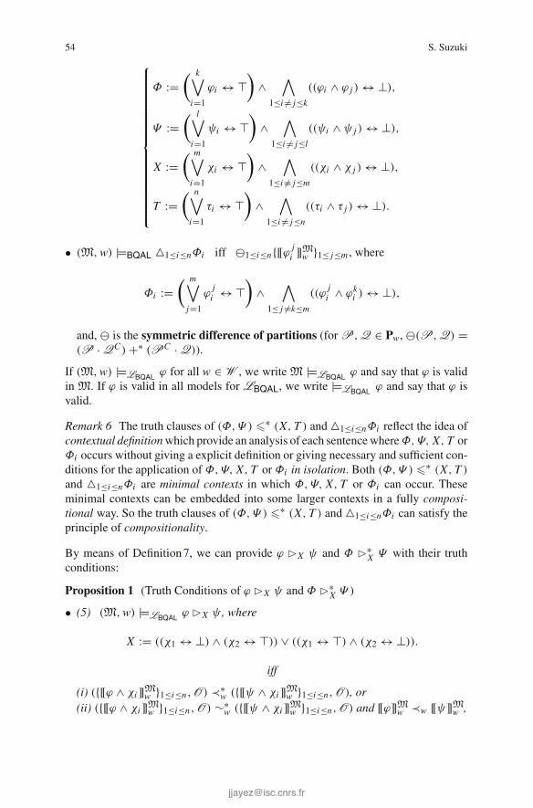
54 S. Suzuki
⎧⎪⎪⎪⎪⎪⎪⎪⎪⎪⎪⎪⎪⎪⎪⎪⎪⎨
⎪⎪⎪⎪⎪⎪⎪⎪⎪⎪⎪⎪⎪⎪⎪⎪⎩
Φ :=( k∨
i=1
ϕi ↔ �)
∧∧
1≤i �= j≤k
((ϕi ∧ ϕ j ) ↔ ⊥),
Ψ :=( l∨
i=1
ψi ↔ �)
∧∧
1≤i �= j≤l
((ψi ∧ ψ j ) ↔ ⊥),
X :=( m∨
i=1
χi ↔ �)
∧∧
1≤i �= j≤m
((χi ∧ χ j ) ↔ ⊥),
T :=( n∨
i=1
τi ↔ �)
∧∧
1≤i �= j≤n
((τi ∧ τ j ) ↔ ⊥).
• (M, w) |=BQAL �1≤i≤nΦi iff �1≤i≤n{[[ϕ ji ]]Mw }1≤ j≤m , where
Φi :=( m∨
j=1
ϕji ↔ �
)∧
∧
1≤ j �=k≤m
((ϕji ∧ ϕk
i ) ↔ ⊥),
and, � is the symmetric difference of partitions (forP,Q ∈ Pw, �(P,Q) =(P · QC ) +∗ (PC · Q)).
If (M, w) |=LBQAL ϕ for all w ∈ W , we write M |=LBQAL ϕ and say that ϕ is validin M. If ϕ is valid in all models for LBQAL, we write |=LBQAL ϕ and say that ϕ isvalid.
Remark 6 The truth clauses of (Φ,Ψ ) �∗ (X, T ) and �1≤i≤nΦi reflect the idea ofcontextual definitionwhich provide an analysis of each sentencewhereΦ,Ψ, X, T orΦi occurs without giving a explicit definition or giving necessary and sufficient con-ditions for the application of Φ,Ψ, X, T or Φi in isolation. Both (Φ,Ψ ) �∗ (X, T )
and �1≤i≤nΦi are minimal contexts in which Φ,Ψ, X, T or Φi can occur. Theseminimal contexts can be embedded into some larger contexts in a fully composi-tional way. So the truth clauses of (Φ,Ψ ) �∗ (X, T ) and �1≤i≤nΦi can satisfy theprinciple of compositionality.
By means of Definition7, we can provide ϕ �X ψ and Φ �∗X Ψ with their truth
conditions:
Proposition 1 (Truth Conditions of ϕ �X ψ and Φ �∗X Ψ )
• (5) (M, w) |=LBQAL ϕ �X ψ , where
X := ((χ1 ↔ ⊥) ∧ (χ2 ↔ �)) ∨ ((χ1 ↔ �) ∧ (χ2 ↔ ⊥)).
iff
(i) ({[[ϕ ∧ χi ]]Mw }1≤i≤n,O) ≺∗w ({[[ψ ∧ χi ]]Mw }1≤i≤n,O), or
(ii) ({[[ϕ ∧ χi ]]Mw }1≤i≤n,O) ∼∗w ({[[ψ ∧ χi ]]Mw }1≤i≤n,O) and [[ϕ]]Mw ≺w [[ψ]]Mw ,

Measurement-Theoretic Foundations of Logic … 55
• (6) (M, w) |=LBQAL Φ �∗X Ψ , where
⎧⎪⎪⎪⎪⎪⎪⎪⎪⎪⎪⎨
⎪⎪⎪⎪⎪⎪⎪⎪⎪⎪⎩
Φ :=( l∨
i=1
ϕi ↔ �)
∧∧
1≤i �= j≤l
((ϕi ∧ ϕ j ) ↔ ⊥),
Ψ :=( m∨
i=1
ψi ↔ �)
∧∧
1≤i �= j≤m
((ψi ∧ ψ j ) ↔ ⊥),
X :=( n∨
i=1
χi ↔ �)
∧∧
1≤i �= j≤n
((χi ∧ χ j ) ↔ ⊥).
iff
(i) {[[χi ]]Mw }1≤i≤n | {[[ϕi ]]Mw }1≤i≤l ≺∗w {[[χi ]]Mw }1≤i≤n | {[[ψi ]]Mw }1≤i≤m, or
(ii) {[[χi ]]Mw }1≤i≤n | {[[ϕi ]]Mw }1≤i≤l ∼∗w {[[χi ]]Mw }1≤i≤n | {[[ψi ]]Mw }1≤i≤m and
{[[ψi ]]Mw }1≤i≤m ⊂∗ {[[ϕi ]]Mw }1≤i≤l .
Remark 7 (Semantic Expressibility in BQAL)
• (3) in Introduction is expressed semantically by (5) in BQAL.• (4) in Introduction is expressed semantically by (6) in BQAL.
5 Syntax (Axiomatisation) of BQAL
5.1 Proof System of BQAL
On the basis of Domotor (1969), we can translate the part of∑
1≤i≤n
Pi =∑
1≤i≤n
Ri
and∑
1≤i≤n
Qi =∑
1≤i≤n
Ti of (D5) of Definition3 into a system of identities among
partitions by means of the following proposition:
Proposition 2 (Symmetric Difference of Partitions)
∑
1≤i≤n
Pi =∑
1≤i≤n
Ri iff�1≤i≤nPi = �1≤i≤nRi
and �1≤i< j≤n (Pi · Pi ) = �1≤i< j≤n(Ri · Ri )
and · · · and �1≤i1<···<in≤n (Pi1 · · ·Pin ) = �1≤i1<···<in≤n(Ri1 · · ·Rin )
By using a syntactic counterpart � of � in Proposition2, we provide BQAL withthe following proof system.
Definition 8 (Proof System of BQAL)
1. all tautologies of sentential logic,2. ((ϕ1 ↔ ϕ2) ∧ (ψ1 ↔ ψ2)) → ((ϕ1 ⇓ ψ1) ↔ (ϕ2 ⇓ ψ2))
(Replacement of Equivalents on ⇓),

56 S. Suzuki
3. ⊥ ⇓ ϕ
(Syntactic Counterpart of (I1)),4. (ϕ ⇓ ψ) → (ψ ⇓ ϕ)
(Syntactic Counterpart of (I2)),5. (ϕ ⇓ ψ) → (¬ψ ⇓ ϕ)
(Syntactic Counterpart of (I3)),6. ((ϕ ∧ χ) ↔ ⊥) → (((ϕ ⇓ ψ) ∧ (ϕ ⇓ χ)) → (ϕ ⇓ (ψ ∨ χ)))
(Syntactic Counterpart of (I4)),7. ((ϕ1 ↔ ϕ2) ∧ (ψ1 ↔ ψ2)) → ((ϕ1 � ψ1) ↔ (ϕ2 � ψ2))
(Replacement of Equivalents on �),8. � � ⊥
(Syntactic Counterpart of (I5)),9. ϕ � ⊥
(Syntactic Counterpart of (I6)),10. (ϕ � ψ) ∨ (ψ � ϕ)
(Syntactic Counterpart of (I7)),11. ((ϕ � ψ) ∧ (ψ � χ)) → (ϕ � χ)
(Syntactic Counterpart of (I8)),12. ((ϕ ⇓ ψ) ∧ ((ϕ ∧ ψ) ↔ ⊥)) → ((ϕ ↔ ⊥) ∨ (ψ ↔ ⊥))
(Syntactic Counterpart of (I9)),13. (((χ ∧ ϕ) ↔ ⊥) ∧ ((χ ∧ ψ) ↔ ⊥)) → ((ϕ � ψ) ↔ ((ϕ ∨ χ) � (ψ ∨ χ)))
(Syntactic Counterpart of (I10)),14. ((χ ⇓ ϕ) ∧ (χ ⇓ ψ) ∧ (χ � ⊥)) → ((ϕ � ψ) ↔ ((ϕ ∧ χ) � (ψ ∧ χ)))
(Syntactic Counterpart of (I11)),15. ((ψ ∧ τ) ↔ ⊥) → (((ϕ � ψ) ∧ (χ � τ)) → ((ϕ ∨ χ) � (ψ ∨ τ)))
(Syntactic Counterpart of (I12)),16. ((ϕ ⇓ χ) ∧ (ψ ⇓ τ)) → (((ϕ ∧ χ) � (ψ ∧ τ)))
(Syntactic Counterpart of (I13)),17. �(α → β) → (�α → �β) (K ),
18.l∧
i=1
m∨
j=1
(ϕi → ψ j ) → ((Ψ, X) �∗ (Φ, X)), where
⎧⎪⎪⎪⎪⎪⎪⎪⎪⎪⎪⎨
⎪⎪⎪⎪⎪⎪⎪⎪⎪⎪⎩
Φ :=( l∨
i=1
ϕi ↔ �)
∧∧
1≤i �= j≤l
((ϕi ∧ ϕ j ) ↔ ⊥),
Ψ :=( m∨
i=1
ψi ↔ �)
∧∧
1≤i �= j≤m
((ψi ∧ ψ j ) ↔ ⊥),
X :=( n∨
i=1
χi ↔ �)
∧∧
1≤i �= j≤n
((χi ∧ χ j ) ↔ ⊥)
(Syntactic Counterpart of (D1)),

Measurement-Theoretic Foundations of Logic … 57
19. ((Φ,Ψ ) ≈∗ (X, Ψ )) → ((Ψ, T ) �∗ (Φ, T )), where
⎧⎪⎪⎪⎪⎪⎪⎪⎪⎨
⎪⎪⎪⎪⎪⎪⎪⎪⎩
Φ := ((ϕ1 ∨ ϕ2) ↔ �) ∧ (ϕ1 ∧ ϕ2) ↔ ⊥),
Ψ := ((ψ1 ↔ ⊥) ∧ (ψ2 ↔ �)) ∨ ((ψ1 ↔ �) ∧ (ψ2 ↔ ⊥)),
X :=( m∨
i=1
χi ↔ �)
∧∧
1≤i �= j≤l
((ϕi ∧ ϕ j ) ↔ ⊥) ∧∧
1≤i �= j≤m
(χi ≈ χ j ),
T :=( n∨
i=1
τi ↔ �)
∧∧
1≤i �= j≤n
((τi ∧ τ j ) ↔ ⊥)
(Syntactic Counterpart of (D2)),20. ((Φ,Ψ ) �∗ (X, T )) ∨ ((X, T ) �∗ (Φ,Ψ )), where
⎧⎪⎪⎪⎪⎪⎪⎪⎪⎪⎪⎪⎪⎪⎪⎪⎪⎨
⎪⎪⎪⎪⎪⎪⎪⎪⎪⎪⎪⎪⎪⎪⎪⎪⎩
Φ :=( k∨
i=1
ϕi ↔ �)
∧∧
1≤i �= j≤k
((ϕi ∧ ϕ j ) ↔ ⊥),
Ψ :=( l∨
i=1
ψi ↔ �)
∧∧
1≤i �= j≤l
((ψi ∧ ψ j ) ↔ ⊥),
X :=( m∨
i=1
χi ↔ �)
∧∧
1≤i �= j≤m
((χi ∧ χ j ) ↔ ⊥),
T :=( n∨
i=1
τi ↔ �)
∧∧
1≤i �= j≤n
((τi ∧ τ j ) ↔ ⊥)
(Syntactic Counterpart of (D3)),21. ((Φ,Ψ ) �∗ (X, T )) → ((T, X) �∗ (Ψ,Φ)), where
⎧⎪⎪⎪⎪⎪⎪⎪⎪⎪⎪⎪⎪⎪⎪⎪⎪⎨
⎪⎪⎪⎪⎪⎪⎪⎪⎪⎪⎪⎪⎪⎪⎪⎪⎩
Φ :=( k∨
i=1
ϕi ↔ �)
∧∧
1≤i �= j≤k
((ϕi ∧ ϕ j ) ↔ ⊥),
Ψ :=( l∨
i=1
ψi ↔ �)
∧∧
1≤i �= j≤l
((ψi ∧ ψ j ) ↔ ⊥),
X :=( m∨
i=1
χi ↔ �)
∧∧
1≤i �= j≤m
((χi ∧ χ j ) ↔ ⊥),
T :=( n∨
i=1
τi ↔ �)
∧∧
1≤i �= j≤n
((τi ∧ τ j ) ↔ ⊥)
(Syntactic Counterpart of (D4)),

58 S. Suzuki
22.
((�1≤i≤nΦi ↔ �1≤i≤nΨi ) ∧ (�1≤i< j≤n(Φi ∧ Φ j ) ↔ �1≤i< j≤n(Ψi ∧ Ψ j )) ∧ · · · ∧
(�1≤i1<···<in≤n(Φi1 ∧ · · · ∧ Φin ) ↔ �1≤i1<···<in≤n(Ψi1 ∧ · · · ∧ Ψin ))∧(�1≤i≤n Xi ↔ �1≤i≤n Ti ) ∧ (�1≤i< j≤n(Xi ∧ X j ) ↔ �1≤i< j≤n(Ti ∧ Tj )) ∧ · · · ∧(�1≤i1<···<in≤n(Xi1 ∧ · · · ∧ Xin ) ↔ �1≤i1<···<in≤n(Ti1 ∧ · · · ∧ Tin ))
)
→(n−1∧
i=1
((Φi , Ψi ) �∗ (Xi , Ti )) → ((Xn, Tn) �∗ (Φn, Ψn))
),
where
⎧⎪⎪⎪⎪⎪⎪⎪⎪⎪⎪⎪⎪⎪⎪⎪⎨
⎪⎪⎪⎪⎪⎪⎪⎪⎪⎪⎪⎪⎪⎪⎪⎩
Φi :=( m1∨
j=1
ϕji ↔ �
)∧
∧
1≤ j �=k≤m1
((ϕji ∧ ϕk
i ) ↔ ⊥),
Ψi :=( m2∨
j=1
ψj
i ↔ �)
∧∧
1≤ j �=k≤m2
((ψj
i ∧ ψki ) ↔ ⊥),
Xi :=( m3∨
j=1
χj
i ↔ �)
∧∧
1≤ j �=k≤m3
((χj
i ∧ χki ) ↔ ⊥),
Ti :=( m4∨
j=1
τj
i ↔ �)
∧∧
1≤ j �=k≤m4
((τj
i ∧ τ ki ) ↔ ⊥)
(Syntactic Counterpart of (D5)),23. (Φ,Ψ ) �∗ (X, Ψ ), where
⎧⎪⎪⎪⎪⎪⎪⎨
⎪⎪⎪⎪⎪⎪⎩
Φ :=( n∨
i=1
ϕi ↔ �)
∧∧
1≤i �= j≤n
((ϕi ∧ ϕ j ) ↔ ⊥),
Ψ := ((ψ1 ↔ ⊥) ∧ (ψ2 ↔ �)) ∨ ((ψ1 ↔ �) ∧ (ψ2 ↔ ⊥)),
X :=( n∨
i=1
χi ↔ �)
∧∧
1≤i �= j≤n
((χi ∧ χ j ) ↔ ⊥) ∧∧
1≤i �= j≤n
(χi ≈ χ j )
(Syntactic Counterpart of (D6)),24. (Φ ∨ ⊥, Ψ ) �∗ (Φ,Ψ ), where
⎧⎪⎨
⎪⎩Φ :=
( n∨
i=1
ϕi ↔ �)
∧∧
1≤i �= j≤n
((ϕi ∧ ϕ j ) ↔ ⊥),
Ψ := ((ψ1 ↔ ⊥) ∧ (ψ2 ↔ �)) ∨ ((ψ1 ↔ �) ∧ (ψ2 ↔ ⊥))
(Syntactic Counterpart of (D7)),

Measurement-Theoretic Foundations of Logic … 59
25. modus ponens.
A proof of ϕ ∈ ΦLBQAL is a finite sequence ofLBQAL-formulae having ϕ as the lastformula such that either each formula is an instance of an axiom or it can be obtainedfrom formulae that appear earlier in the sequence by applying a modus ponens. Ifthere is a proof of ϕ, we write �BQAL ϕ.
Remark 8 (Behaviour and Structure) The proof system of BQAL has no syntacticcounterpart of (I14) that is satisfied in M of LBQAL of Definition6. For LBQALis not so fine-grained as to express it. However, it is not a defect of BQAL. ForBQAL is designed to capture behaviour about � and �∗, whereas (I14) states theArchimedeanity that is a mere structural property required for the existence of afinitely additive probability measure.
5.2 Theorems and Their Interpretations
BQAL has nontrivial and good properties. Among them, first we show the followingbasic facts:
Proposition 3 (Strict Weak Order (�T )) Suppose that
T :=( n∨
i=1
τi ↔ �)
∧∧
1≤i �= j≤n
((τi ∧ τ j ) ↔ ⊥).
The following then hold:
(7) �BQAL (ϕ �T ψ) → ¬(ψ �T ϕ),
(8) �BQAL (¬(ϕ �T ψ) ∧ ¬(ψ �T χ)) → ¬(ϕ �T χ).
Remark 9 (Asymmetricity, Negative Transitivity and Strict Weak Order)
• (7) states that a being-a-better-answer-than relation satisfies asymmetricity.• (8) states that a being-a-better-answer-than relation satisfies negative transitivity.• (7) and (8) imply that a being-a-better-answer-than relation is a strict weak order.
Proposition 4 (Strict Weak Order (�∗T )) Suppose that

60 S. Suzuki
⎧⎪⎪⎪⎪⎪⎪⎪⎪⎪⎪⎪⎪⎪⎪⎪⎪⎨
⎪⎪⎪⎪⎪⎪⎪⎪⎪⎪⎪⎪⎪⎪⎪⎪⎩
Φ :=( k∨
i=1
ϕi ↔ �)
∧∧
1≤i �= j≤k
((ϕi ∧ ϕ j ) ↔ ⊥),
Ψ :=( l∨
i=1
ψi ↔ �)
∧∧
1≤i �= j≤l
((ψi ∧ ψ j ) ↔ ⊥),
X :=( m∨
i=1
χi ↔ �)
∧∧
1≤i �= j≤m
((χi ∧ χ j ) ↔ ⊥),
T :=( n∨
i=1
τi ↔ �)
∧∧
1≤i �= j≤n
((τi ∧ τ j ) ↔ ⊥)
The following then hold:
(9) �BQAL (Φ �∗T Ψ ) → ¬(Ψ �∗
T Φ),
(10) �BQAL (¬(Φ �∗T Ψ ) ∧ ¬(Ψ �∗
T X)) → ¬(Φ �∗T X).
Remark 10 (Strict Weak Order) (9) and (10) imply that a being-a-better-question-than relation is also a strict weak order.
Now we show one of essential facts in comparing answers to a given question:
Proposition 5 (Incompatible Cells and Betterness of Answers) Suppose that
X :=( n∨
i=1
χi ↔ �)
∧∧
1≤i �= j≤n
((χi ∧ χ j ) ↔ ⊥),
and that, for any p, q (0 ≤ q < p ≤ n), DC(p,q)(ϕ, ψ, X) is defined as thedisjunction of all conjunctions:
n∧
i=1
(δi ((ϕ ∧ χi ) ↔ ⊥) ∧ εi ((ψ ∧ χi ) ↔ ⊥)))
such that exactly p of the δi’s and q of εi’s, are the empty symbol strings, the rest ofthem being ¬’s, and that
DDC(ϕ, ψ, X) := DC(1,0)(ϕ, ψ, X) ∨ DC(2,0)(ϕ, ψ, X) ∨ · · ·∨DC(n,n−2)(ϕ, ψ, X) ∨ DC(n,n−1)(ϕ, ψ, X).
The following then holds:
(11) �BQAL
⎛
⎝DDC(ϕ, ψ, X) ∧∧
1≤i �= j≤n
(χi ≈ χ j )
⎞
⎠ → (ϕ �X ψ).

Measurement-Theoretic Foundations of Logic … 61
Remark 11 (11) implies that a question that can be incompatible with more cells ofa given question is a better answer to it if all cells of it are equiprobable.
Next we show one of essential facts in comparing questions on a mutually exclusiveand exhaustive set of hypotheses:
Proposition 6 (Fine-Grainedness and Betterness of Questions) Suppose that
⎧⎪⎪⎪⎪⎪⎪⎪⎪⎪⎪⎨
⎪⎪⎪⎪⎪⎪⎪⎪⎪⎪⎩
Φ :=( l∨
i=1
ϕi ↔ �)
∧∧
1≤i �= j≤l
((ϕi ∧ ϕ j ) ↔ ⊥),
Ψ :=( m∨
i=1
ψi ↔ �)
∧∧
1≤i �= j≤m
((ψi ∧ ψ j ) ↔ ⊥),
X :=( n∨
i=1
χi ↔ �)
∧∧
1≤i �= j≤n
((χi ∧ χ j ) ↔ ⊥), where m < l < n.
The following then holds:
(12) �BQAL
( ∧
1≤i �= j≤l
(ϕi ≈ ϕ j ) ∧∧
1≤i �= j≤m
(ψi ≈ ψ j ) ∧∧
1≤i �= j≤n
(χi ≈ χ j )
)→ (Φ �∗
X Ψ ).
Remark 12 (12) implies that a more fine-grained question is a better question on amutually exclusive and exhaustive set of hypotheses if the questions and the hypoth-esis set each have their equiprobable cells.
6 Metalogic of BQAL
It is a routine to prove the soundness of BQAL.
Theorem 3 (Soundness) For any ϕ ∈ ΦLBQAL , if �BQAL ϕ, then |=BQAL ϕ.
We now turn to the task of proving the completeness of BQAL. We prove it byusing the ideas of Segerberg (1971) and modifying filtration in such a way thatcompleteness can be established by Theorem1 (Representation Theorem for �) andTheorem2 (Representation Theorem for �∗). We cannot go into detail because oflimited space, but the outline of the proof is as follows: We begin by defining somenew concepts.
Definition 9 (Stuffedness and Value Formula) Suppose that Θ is a set of formulaesuch that Θ is closed under subformulae. Let
Δ := {ϕ : for someψ, ϕ � ψ ∈ Θ orψ � ϕ) ∈ Θ}, andΔ∗
1 × Δ∗2 := {(Φ,Ψ ) : for some (X, T ), (Φ,Ψ ) �∗ (X, T ) ∈ Θ or (X, T ) �∗ (Φ,Ψ ) ∈ Θ},

62 S. Suzuki
and let Δ′ (Δ∗′1 and Δ∗′
2 respectively) be the closure of Δ (Δ∗1 and Δ∗
2 respectively)under Boolean compounds. If Θ also satisfies the condition that ϕ � ψ ∈ Θ , forany ϕ,ψ ∈ Δ′ and that (Φ,Ψ ) �∗ (X, T ), for any (Φ,Ψ ), (X, Y ) ∈ Δ∗
1 × Δ∗2, we
say that Θ is stuffed. The formulae in Δ′,Δ∗′1 or Δ∗′
2 are called the value formulaeof Θ .
Remark 13 There is no occurrence of � and �∗ in value formulae.
Definition 10 (Base and Logical Finiteness) We say that Λ0 ⊂ ΦLBQAL is a base(with respect to BQAL) for Λ ⊂ ΦLBQAL if for any ϕ ∈ Λ there is some ϕ0 ∈ Λ0such that �BQAL ϕ ↔ ϕ0. We say that Λ is logically finite (with respect to BQAL)if there is a finite base for Λ.
Then we can prove the next lemma:
Lemma 1 (Logical Finiteness) If Λ ⊂ ΦLBQAL is a finite set closed under subfor-mulae, and if Θ is the smallest stuffed superset of Λ, then Θ is logically finite.
We define BQAL-maximal consistency as follows:
Definition 11 (BQAL-Maximal Consistent Set) A finite set {ϕ1, . . . , ϕn} ⊂ ΦLBQALisBQAL-consistent iff�BQAL ¬(ϕ1∧. . .∧ϕn). An infinite set of formulae isBQAL-consistent iff all of its finite subsets are BQAL-consistent. Γ ⊂ ΦLBQAL is a BQAL-maximal consistent set iff it is BQAL-consistent and for any ϕ /∈ Γ , Γ ∪ {ϕ} isBQAL-inconsistent.
A canonical model for the modal part of BQAL is defined as follows:
Definition 12 (Canonical Model for Modal Part) We define UC := (X C , RC , V C )
as a canonical model for the modal part of BQAL in which
• X C := {Γ ⊂ ΦLBQAL : Γ is BQAL-maximal consistent},• for any Γ,Δ ∈ X C , R(Γ,Δ) iff for any α ∈ ΦLBQAL , if �α ∈ Γ , then α ∈ Δ,and
• for any Γ ∈ X C ,
V C (Γ )(s) :={
true if s ∈ Γ,
false otherwise.
We define an equivalence relation modulo Θ on X C as follows:
Definition 13 (Equivalence Relation) Let Θ be a stuffed set of formulae that arelogically finite with respect to BQAL. We define, for Γ,Δ ∈ X C ,
Γ ≡Θ Δ iff Γ ∩ Θ = Δ ∩ Θ.
Then, ≡Θ is an equivalence relation modulo Θ on X C . We write [Γ ]Θ for theequivalence class of Γ under ≡Θ .
A filtration of UC through Θ is defined as follows:
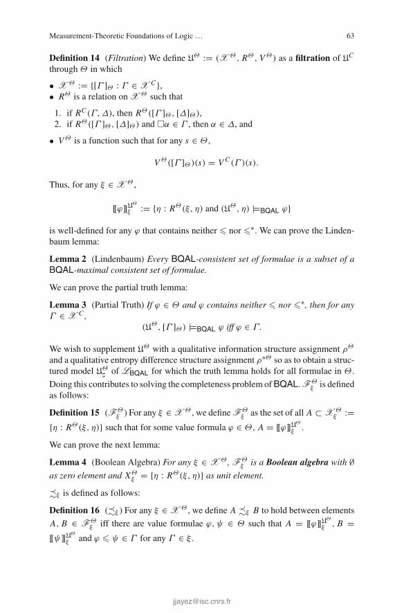
Measurement-Theoretic Foundations of Logic … 63
Definition 14 (Filtration) We define UΘ := (X Θ, RΘ, V Θ) as a filtration of UC
through Θ in which
• X Θ := {[Γ ]Θ : Γ ∈ X C },• RΘ is a relation onX Θ such that
1. if RC (Γ,Δ), then RΘ([Γ ]Θ, [Δ]Θ),2. if RΘ([Γ ]Θ, [Δ]Θ) and �α ∈ Γ , then α ∈ Δ, and
• V Θ is a function such that for any s ∈ Θ ,
V Θ([Γ ]Θ)(s) = V C (Γ )(s).
Thus, for any ξ ∈ X Θ ,
[[ϕ]]UΘ
ξ := {η : RΘ(ξ, η) and (UΘ, η) |=BQAL ϕ}
is well-defined for any ϕ that contains neither � nor �∗. We can prove the Linden-baum lemma:
Lemma 2 (Lindenbaum) Every BQAL-consistent set of formulae is a subset of aBQAL-maximal consistent set of formulae.
We can prove the partial truth lemma:
Lemma 3 (Partial Truth) If ϕ ∈ Θ and ϕ contains neither � nor �∗, then for anyΓ ∈ X C ,
(UΘ, [Γ ]Θ) |=BQAL ϕ iff ϕ ∈ Γ.
We wish to supplement UΘ with a qualitative information structure assignment ρΘ
and a qualitative entropy difference structure assignment ρ∗Θ so as to obtain a struc-tured model UΘ
� of LBQAL for which the truth lemma holds for all formulae in Θ .
Doing this contributes to solving the completeness problem ofBQAL.FΘξ is defined
as follows:
Definition 15 (FΘξ ) For any ξ ∈ X Θ , we defineFΘ
ξ as the set of all A ⊂ X Θξ :=
{η : RΘ(ξ, η)} such that for some value formula ϕ ∈ Θ , A = [[ϕ]]UΘ
ξ .
We can prove the next lemma:
Lemma 4 (Boolean Algebra) For any ξ ∈ X Θ , FΘξ is a Boolean algebra with ∅
as zero element and XΘξ = {η : RΘ(ξ, η)} as unit element.
�ξ is defined as follows:
Definition 16 (�ξ ) For any ξ ∈ X Θ , we define A �ξ B to hold between elements
A, B ∈ FΘξ iff there are value formulae ϕ,ψ ∈ Θ such that A = [[ϕ]]UΘ
ξ , B =[[ψ]]UΘ
ξ and ϕ � ψ ∈ Γ for any Γ ∈ ξ .

64 S. Suzuki
We can prove the next lemma:
Lemma 5 (�ξ and �) For any value formula ϕ,ψ ∈ Θ and any ξ ∈ X Θ ,
[[ϕ]]UΘ
ξ �ξ [[ψ]]UΘ
ξ iff, for any Γ ∈ ξ , ϕ � ψ ∈ Γ .
Since we assumed that Θ is logically finite, X Θ is finite. Hence for any ξ ∈ X Θ ,FΘ
ξ is finite. So the next lemma follows from Lemma5.
Lemma 6 (Satisfaction of (I1)–(I14)) For any ξ ∈ X Θ , �ξ on FΘξ satisfies (I1)–
(I14).
Remark 14 Since FΘξ is finite, (I14) is automatically satisfied.
The next corollary follows from Theorem1 (Representation Theorem for �), Lem-mas4 and 6.
Corollary 1 (Representation on FΘξ ) For any ξ ∈ X Θ , (X Θ
ξ ,FΘξ ,�ξ ,⊥⊥ ξ ) is
a qualitative information structure, and there exists a finitely additive probabilitymeasure Pξ : FΘ
ξ → IR such that (X Θξ ,FΘ
ξ , Pξ ) is a finitely additive probability
space, and for any A, B ∈ FΘξ the conditions (i)–(iii) of Theorem1 hold.
We continue the proof about �∗ as well as �.
Definition 17 (PΘξ ) For any ξ ∈ X Θ , we define PΘ
ξ as the set of all partitions P
over X Θξ := {η : RΘ(ξ, η)} such that for some value formulae ϕ1, . . . , ϕn ∈ Θ ,
P := {[[ϕi ]]UΘ
ξ }1≤i≤n , where
n⋃
i=1
[[ϕi ]]UΘ
ξ = X Θξ and
⋂
1≤i �= j≤n
(([[ϕi ]]UΘ
ξ ∩ [[ϕ j ]]UΘ
ξ ) = ∅).
�ξ is defined as follows:
Definition 18 (�∗ξ ) For any ξ ∈ X Θ , we define (P,Q) �∗
ξ (R,T ) to hold
between elements P,Q,R,T ∈ PΘξ iff there are value formulae ϕ1, . . . , ϕk, ψ1,
. . . , ψl , χ1 . . . , χm, τ1, . . . , τn ∈ Θ such that P = {[[ϕi ]]UΘ
ξ }1≤i≤k ,Q ={[[ψi ]]UΘ
ξ }1≤i≤l , R = {[[χi ]]UΘ
ξ }1≤i≤m , T = {[[τi ]]UΘ
ξ }1≤i≤n and (Φ,Ψ ) �∗(X, T ) ∈ Γ for any Γ ∈ ξ , where

Measurement-Theoretic Foundations of Logic … 65
⎧⎪⎪⎪⎪⎪⎪⎪⎪⎪⎪⎪⎪⎪⎪⎪⎪⎨
⎪⎪⎪⎪⎪⎪⎪⎪⎪⎪⎪⎪⎪⎪⎪⎪⎩
Φ :=( k∨
i=1
ϕi ↔ �)
∧∧
1≤i �= j≤k
((ϕi ∧ ϕ j ) ↔ ⊥),
Ψ :=( l∨
i=1
ψi ↔ �)
∧∧
1≤i �= j≤l
((ψi ∧ ψ j ) ↔ ⊥),
X :=( m∨
i=1
χi ↔ �)
∧∧
1≤i �= j≤m
((χi ∧ χ j ) ↔ ⊥),
T :=( n∨
i=1
τi ↔ �)
∧∧
1≤i �= j≤n
((τi ∧ τ j ) ↔ ⊥).
We can prove the next lemma:
Lemma 7 (�ξ and �) For any value formula ϕ1, . . . , ϕk, ψ1, . . . , ψl , χ1 . . . , χm,
τ1, . . . , τn ∈ Θ and any ξ ∈ X Θ , ({[[ϕi ]]UΘ
ξ }1≤i≤k, {[[ψi ]]UΘ
ξ }1≤i≤l) �ξ
({[[χi ]]UΘ
ξ }1≤i≤m, {[[τi ]]UΘ
ξ }1≤i≤n) iff, for any Γ ∈ ξ , (Φ,Ψ ) �∗ (X, T ) ∈ Γ .
The next lemma follows from Lemma7.
Lemma 8 (Satisfaction of (D1)–(D7))For any ξ ∈ X Θ , �∗ξ on ∈ PΘ
ξ ×PΘξ satisfies
(D1)–(D7).
The next corollary follows from Theorem2 (Representation Theorem for �∗) andLemma8.
Corollary 2 (Representation on PΘξ ) For any ξ ∈ X Θ , (X Θ, PΘ
ξ ,�∗ξ ,⊥⊥ ∗
ξ ) is a
finite qualitative entropy difference structure and there exists a function H : PΘξ →
IR satisfying the conditions (D1) − (D7) of Theorem2.
U� is defined as follows:
Definition 19 (UΘ� )WedefineUΘ
� as (X Θ, RΘ, V Θ, ρΘ, ρ∗Θ),whereρΘ is a qual-
itative information structure assignment that assigns to each ξ ∈ X Θ a qualitativeinformation structure (X Θ
ξ ,FΘξ ,�ξ ,⊥⊥ ξ ) in which
• X Θξ := {ξ ′ : RΘ(ξ, ξ ′)},
• FΘξ is a Boolean algebra of subsets of X Θ
ξ with ∅ as zero element and X Θξ as
unit element,• �ξ is a relation onFΘ
ξ that satisfies all of the conditions (I1)–(I14) of Definition1,
• ⊥⊥ ξ is probabilistic independence relation onFΘξ ,
and where ρ∗Θ is a qualitative entropy difference structure assignment that assignsto each ξ ∈ X Θ a qualitative entropy difference structure (X Θ
ξ , PΘξ ,�∗
ξ ,⊥⊥ ∗ξ ) in
which
• PΘξ is an algebra of partitions over X Θ
ξ ,

66 S. Suzuki
• �∗ξ is a relation on PΘ
ξ × PΘξ that satisfies all of the conditions (D1)–(D7) of
Definition3, and• ⊥⊥ ∗
ξ is probabilistic independence relation on PΘξ .
We can prove the full truth lemma:
Lemma 9 (Full Truth) For any ϕ ∈ Θ and any Γ ∈ X C ,
(UΘ� , [Γ ]Θ) |=BQAL ϕ iff ϕ ∈ Γ.
Remark 15 This lemma is the announced improvement of Lemma3.
We can prove the completeness of BQAL as follows:
Theorem 4 (Completeness) For any ϕ ∈ ΦLBQAL , if |=BQAL ϕ, then �BQAL ϕ.
Proof Suppose that �BQAL ϕ0. Then {¬ϕ0} is a BQAL-consistent set. By Lemma2,{¬ϕ0} is a subset of a BQAL-maximal consistent set Γ . Evidently, ϕ0 /∈ Γ . LetΨ be the set of subformulae of BQAL which is finite and let Θ be the smalleststuffed extension of Ψ . By Lemma1, Θ is logically finite with respect to BQAL. IfUΘ
� is constructed as above, it follows from Lemma9 that (UΘ� , [Γ ]Θ) �|=BQAL ϕ0.
Therefore, �|=BQAL ϕ0.
7 Application of BQAL to Examples 2 and 3
7.1 Example 2 Reconsidered
Suppose that ⎧⎨
⎩
J := John is sick.M := Mary is sick.S := Sue is sick.,
and that
X := (((J ∧ M ∧ S) ∨ · · · ∨ (¬J ∧ ¬M¬S)) ↔ �)
∧(((J ∧ M ∧ S) ∧ (J ∧ M ∧ ¬S)) ↔ ⊥) ∧ · · · ∧ (((¬J ∧ M ∧ ¬S) ∧ (¬J ∧ ¬M ∧ ¬S)) ↔ ⊥).
The next then follows from Proposition5:
�BQAL (¬(((J ∧ M ∧ S) ∧ (J ∧ M)) ↔ ⊥) ∧ ¬(((J ∧ M ∧ S) ∧ S) ↔ ⊥)
∨ · · · ∨ (((¬J ∧ ¬M¬S) ∧ (J ∧ M)) ↔ ⊥) ∧ (((¬J ∧ ¬M ∧ ¬S) ∧ S) ↔ ⊥)
∧((J ∧ M ∧ S) ≈ (J ∧ M ∧ ¬S)) ∧ · · · ∧ ((¬J ∧ ¬M ∧ S) ≈ (¬J ∧ ¬M ∧ ¬S)))
→ ((J ∧ M) �X S).
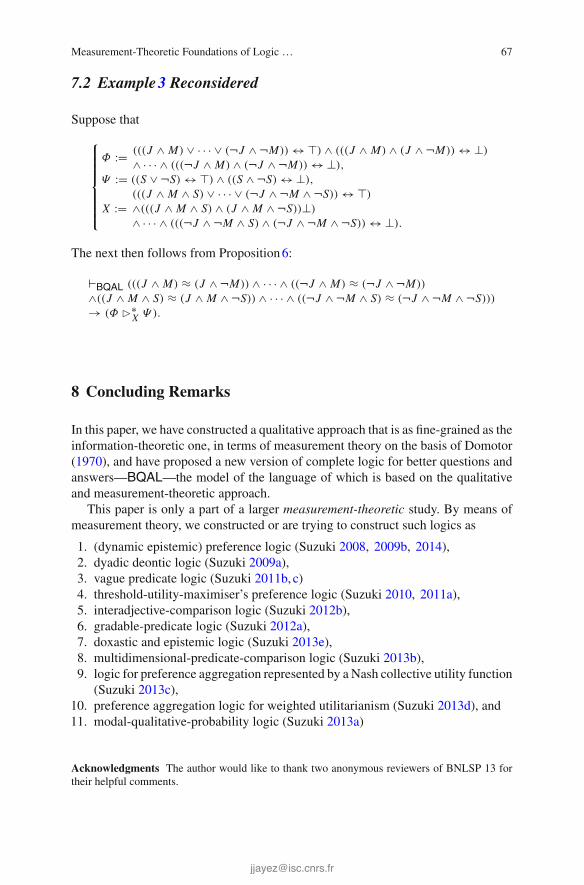
Measurement-Theoretic Foundations of Logic … 67
7.2 Example 3 Reconsidered
Suppose that
⎧⎪⎪⎪⎪⎪⎪⎨
⎪⎪⎪⎪⎪⎪⎩
Φ := (((J ∧ M) ∨ · · · ∨ (¬J ∧ ¬M)) ↔ �) ∧ (((J ∧ M) ∧ (J ∧ ¬M)) ↔ ⊥)
∧ · · · ∧ (((¬J ∧ M) ∧ (¬J ∧ ¬M)) ↔ ⊥),
Ψ := ((S ∨ ¬S) ↔ �) ∧ ((S ∧ ¬S) ↔ ⊥),
X :=(((J ∧ M ∧ S) ∨ · · · ∨ (¬J ∧ ¬M ∧ ¬S)) ↔ �)
∧(((J ∧ M ∧ S) ∧ (J ∧ M ∧ ¬S))⊥)
∧ · · · ∧ (((¬J ∧ ¬M ∧ S) ∧ (¬J ∧ ¬M ∧ ¬S)) ↔ ⊥).
The next then follows from Proposition6:
�BQAL (((J ∧ M) ≈ (J ∧ ¬M)) ∧ · · · ∧ ((¬J ∧ M) ≈ (¬J ∧ ¬M))
∧((J ∧ M ∧ S) ≈ (J ∧ M ∧ ¬S)) ∧ · · · ∧ ((¬J ∧ ¬M ∧ S) ≈ (¬J ∧ ¬M ∧ ¬S)))
→ (Φ �∗X Ψ ).
8 Concluding Remarks
In this paper, we have constructed a qualitative approach that is as fine-grained as theinformation-theoretic one, in terms of measurement theory on the basis of Domotor(1970), and have proposed a new version of complete logic for better questions andanswers—BQAL—the model of the language of which is based on the qualitativeand measurement-theoretic approach.
This paper is only a part of a larger measurement-theoretic study. By means ofmeasurement theory, we constructed or are trying to construct such logics as
1. (dynamic epistemic) preference logic (Suzuki 2008, 2009b, 2014),2. dyadic deontic logic (Suzuki 2009a),3. vague predicate logic (Suzuki 2011b, c)4. threshold-utility-maximiser’s preference logic (Suzuki 2010, 2011a),5. interadjective-comparison logic (Suzuki 2012b),6. gradable-predicate logic (Suzuki 2012a),7. doxastic and epistemic logic (Suzuki 2013e),8. multidimensional-predicate-comparison logic (Suzuki 2013b),9. logic for preference aggregation represented by a Nash collective utility function
(Suzuki 2013c),10. preference aggregation logic for weighted utilitarianism (Suzuki 2013d), and11. modal-qualitative-probability logic (Suzuki 2013a)
Acknowledgments The author would like to thank two anonymous reviewers of BNLSP 13 fortheir helpful comments.

68 S. Suzuki
References
Domotor, Z. (1969). Probabilistic relational structures and their applications. Technical report No.144, Institute for Mathematical Studies in the Social Sciences, Stanford University.
Domotor, Z. (1970). Qualitative information and entropy structures. In J. Hintikka & P. Suppes(Eds.), Information and inference (pp. 148–194). Dordrecht: Reidel.
Groenendijk, J., &Stokhof,M. (1984). On the semantics of questions and the pragmatics of answers.In F. Landman&F.Veltman (Eds.),Varieties of formal semantics (pp. 143–170). Dordrecht: Foris.
Hölder, O. (1901). Die Axiome der Quantität und die Lehre vom Mass. Berichte über die Verhand-lungen der Königlich Sächsischen Gesellschaft der Wissenschaften zu Leipzig. Mathematisch-Physikalische Klasse, 53, 1–64.
Krantz, D. H., et al. (1971). Foundations of measurement (Vol. 1). New York: Academic Press.Luce, R. D., et al. (1990). Foundations of measurement (Vol. 3). San Diego: Academic Press.Roberts, F. S. (1979). Measurement theory. Reading: Addison-Wesley.Segerberg, K. (1971). Qualitative probability in a modal setting. In J. E. Fenstad (Ed.), Proceedings
of the second Scandinavian logic symposium (pp. 341–352). Amsterdam: North-Holland.Suppes, P., et al. (1989). Foundations of measurement (Vol. 2). San Diego: Academic Press.Suzuki, S. (2008). Preference logic and its measurement-theoretic semantics. In Electronic Pro-
ceedings of the 8th Conference on Logic and the Foundations of Game and Decision Theory(LOFT 2008), Paper No. 42.
Suzuki, S. (2009a). Measurement-theoretic foundation of preference-based dyadic deontic logic.In X. He, et al. (Eds.), Proceedings of the Second International Workshop on Logic, Rationality,and Interaction (LORI-II). LNCS (Vol. 5834, pp. 278–291). Heidelberg: Springer.
Suzuki, S. (2009b). Prolegomena to dynamic epistemic preference logic. In H. Hattori, et al. (Eds.),New Frontiers in artificial intelligence. LNCS (Vol. 5447, pp. 177–192). Heidelberg: Springer.
Suzuki, S. (2010). Prolegomena to threshold utility maximiser’s preference logic. In ElectronicProceedings of the 9th Conference on Logic and the Foundations of Game and Decision Theory(LOFT 2010), Paper No. 44.
Suzuki, S. (2011a). Ameasurement-theoretic foundation of threshold utilitymaximiser’s preferencelogic. Journal of Applied Ethics and Philosophy, 3, 17–25.
Suzuki, S. (2011b). Measurement-theoretic foundations of probabilistic model of JND-based vaguepredicate logic. In H. van Ditmarsch, et al. (Eds.), Proceedings of the Third International Work-shop on Logic, Rationality, and Interaction (LORI-III). LNCS (Vol. 6953, pp. 272–285). Heidel-berg: Springer.
Suzuki, S. (2011c). Prolegomena to salient-similarity-based vague predicate logic. In T. Onada,et al. (Eds.), New Frontiers in artificial intelligence. LNCS (Vol. 6797, pp. 75–89). Heidelberg:Springer.
Suzuki, S. (2012a).Measurement-theoretic foundations of gradable-predicate logic. InM.Okumura,et al. (Eds.), New Frontiers in artificial intelligence. LNCS (Vol. 7258, pp. 82–95). Heidelberg:Springer.
Suzuki, S. (2012b). Measurement-theoretic foundations of interadjective-comparison logic. InA. Aguilar-Guevara, et al. (Eds.), Proceedings of Sinn und Bedeutung 16 (Vol. 2, pp. 571–584).Cambridge: MIT Working Papers in Linguistics.
Suzuki, S. (2013a). Epistemic modals, qualitative probability, and nonstandard probability. InM. Aloni, et al. (Eds.), Proceedings of the 19th Amsterdam Colloquium (AC 2013) (pp. 211–218).
Suzuki, S. (2013b). Measurement-theoretic bases of multidimensional-predicate logic. Manuscript.Suzuki, S. (2013c). Measurement-theoretic foundations of many-sorted preference aggregationlogic for Nash collective utility function. Manuscript.
Suzuki, S. (2013d). Measurement-theoretic foundations of preference aggregation logic forweighted utilitarianism. In T. Yamada (Ed.), Electronic Post-Proceedings of the Third Inter-national Workshop on Philosophy and Ethics of Social Reality (SOCREAL 2013) (pp. 68–79).

Measurement-Theoretic Foundations of Logic … 69
Suzuki, S. (2013e). Remarks on decision-theoretic foundations of doxastic and epistemic logic(revised version). Studies in Logic, 6, 1–12.
Suzuki, S. (2014). Measurement-theoretic foundations of dynamic epistemic preference logic. InE.McCready, et al. (Eds.),Formal approaches to semantics and pragmatics. Studies in Linguisticsand Philosophy (Vol. 95, pp. 295–324). Heidelberg: Springer.
van Rooij, R. (2009). Comparing questions and answers: A bit of logic, a bit of language, andsome bits of information. In G. Sommaruga (Ed.), Formal theories of information: From Shan-non to semantic information theory and general concepts of information. LNCS (Vol. 5363,pp. 161–192). Heidelberg: Springer.

Conditionals, Conditional Probabilities,and Conditionalization
Stefan Kaufmann
Abstract Philosophers investigating the interpretation and use of conditional sen-tences have long been intrigued by the intuitive correspondence between the proba-bility of a conditional ‘if A, then C’ and the conditional probability of C , given A.Attempts to account for this intuition within a general probabilistic theory of belief,meaning and use have been plagued by a danger of trivialization, which has provento be remarkably recalcitrant and absorbed much of the creative effort in the area.But there is a strategy for avoiding triviality that has been known for almost as longas the triviality results themselves. What is lacking is a straightforward integrationof this approach in a larger framework of belief representation and dynamics. Thispaper discusses some of the issues involved and proposes an account of belief updateby conditionalization.
Keywords Conditionals · Probability · Conditional probability · StalnakerBernoulli Models
1 Introduction
Most contemporary theories of the interpretation of conditionals are inspired byRamsey’s (1929) paraphrase of the mental process involved in their interpretation,known as the Ramsey Test (RT):
Thanks to Hans-Christian Schmitz and Henk Zeevat for organizing the ESSLLI 2014 workshopon Bayesian Natural-Language Semantics and Pragmatics, where I presented an early versionof this paper. Other venues at which I presented related work include the research group “Whatif” at the University of Konstanz and the Logic Group at the University of Connecticut. I amgrateful to the audiences at all these events for stimulating discussion and feedback. Thanksalso to Hans-Christian Schmitz and Henk Zeevat for their patience during the preparation ofthis manuscript. All errors and misrepresentations are my own.
S. Kaufmann (B)
University of Connecticut, Mansfield, USAe-mail: [email protected]
© Springer International Publishing Switzerland 2015H. Zeevat and H.-C. Schmitz (eds.), Bayesian Natural Language Semanticsand Pragmatics, Language, Cognition, and Mind 2,DOI 10.1007/978-3-319-17064-0_4
71

72 S. Kaufmann
(RT) If two people are arguing ‘If A will C?’ and are both in doubt as to A, they areadding A hypothetically to their stock of knowledge and arguing on that basisabout C…We can say they are fixing their degrees of belief in C given A.
For all its intuitive appeal, (RT) is too general andunderspecified to be operationalizedin a concrete theoretical approach. To turn it into a definition, one has to flesh outseveral abstract ideas it mentions. Most crucially, this concerns the notions of stockof knowledge, adding A temporarily, and degrees of belief .
In this paper I explore oneparticularway to read (RT), viz. a versionof probabilisticsemantics inspired byRamsey and developed by Jeffrey (1964), Adams (1965, 1975),and many subsequent authors. The basic ingredients are familiar from propositionallogic. Sentences denote propositions, modeled as sets of possible worlds. Epistemicstates (Ramsey’s “stocks of knowledge”) are represented in terms of (subjective)probabilities. The addition of the antecedent proceeds by conditionalization.
Regarding the latter point, another question that needs to be addressed is whetherone and the same update operation is appropriate for all conditionals. Conditional-ization on a proposition is typically interpreted as modeling the process of learning(hence coming to believe) that the proposition is true. However, there are well-known examples of conditionals in which the relevant supposition is intuitively thatthe antecedent is true without its truth being known to the speaker. This can beillustrated with examples whose antecedents or consequents explicitly deny the rel-evant belief, such as ‘if it’s raining and I don’t know it. . .’. Examples of this kindare generally problematic for theories—whether probabilistic or not—which rely ona single operation to represent the hypothetical reasoning involved. I return to thisissue towards the end of the paper, having introduced a formal framework in whichthe relevant distinction can be accounted for.
2 Probability Models
To get things started, I begin with a fairly simple model-theoretic interpretation. Fornow the goal is to stay close to the standard possible-worlds apparatus of propositionallogic, adding only the structure required to model probability judgments. The setupI introduce in this subsection will ultimately not work, as we will see below. But itis a good place to start.
I assume that sentences of English are mapped to expressions of the standardlanguage of propositional logic, and spell out the formal details in terms of the latter.Let A be a set of atomic propositional letters, and L0
A be the smallest set containingA and closed under negation and conjunction. I write ‘ϕ’ and ‘ϕψ’ for the negation

Conditionals, Conditional Probabilities, and Conditionalization 73
of ϕ and the conjunction of ϕ and ψ, respectively. A probability model is a standardpossible-worlds model for L0
A, augmented with a probability measure.
Definition 1 (Probability model) A probability model for language L0A is a tuple
〈Ω,F ,Pr, V 〉, where1:• Ω is a non-empty set (of possible worlds);• F is a σ-algebra on Ω;• Pr is a probability measure on F ;• V is a function mapping sentences to characteristic functions of elements of F ,subject to the following conditions, for all ϕ,ψ ∈ L0
A and ω ∈ Ω:
V (ϕ)(ω) = 1 − V (ϕ)(ω)
V (ϕψ)(ω) = V (ϕ)(ω) × V (ψ)(ω)
To relate the terminology familiar from possible-worlds semantics to the statisticaljargon of probability theory, we can equate possible worlds with outcomes and setsof possible worlds (i.e., propositions) with events. Definition1 follows the prac-tice, common in probability theory, of separating the representations of the space ofoutcomes and the algebra on which the measure is defined (here Ω and F , respec-tively). There are good philosophical reasons for doing this, but for the purposes ofthis paper, no harm is done by assuming for simplicity that F is the powerset of Ω .It then follows without further stipulation that all propositions denoted by sentencesare in the domain of the probability function.
Note that V maps sentences not to sets of worlds, but to their characteristic func-tions. Statistically speaking, those sentence denotations are indicator variables—aspecial kind of random variables whose range is restricted to the set {0, 1} . Inthe present context this perspective was first proposed by Jeffrey (1991) and fur-ther developed by Stalnaker and Jeffrey (1994). The motivation for modeling thedenotations of sentences in this way will become clear below. It is important in theformal setup, but I will occasionally collapse talk of sets of worlds and talk of theircharacteristic functions where concepts rather than implementation are at stake.
The function Pr assigns probabilities to propositions, not sentences, but basedon it we can assign probabilities to sentences indirectly as the expectations of theirvalues. Generally speaking (and not just in the case of variables with range {0, 1}),the expectation of a random variable is the weighted sum of its values, where theweights are the probabilities that it takes those values.
1A σ-algebra on Ω is a non-empty set of subsets of Ω that is closed under complements andcountable unions. A probability measure on F is a countably additive function from F to the realinterval [0, 1] such that Pr(Ω) = 1.

74 S. Kaufmann
Definition 2 (Expectation) Let θ : Ω �→ R be a random variable. The expectationof θ relative to a probability function Pr is defined as follows2:
E[θ] =∑
x∈range(θ)
x × Pr(θ = x).
For the purposes of interpreting the language L0A, the relevant variable for a given
sentence ϕ is its interpretation V (ϕ).
Definition 3 (Probabilities of sentences) Given a probability model for L0A (see
Definition1), a function P maps sentences to real numbers as follows:
P(ϕ) = E[V (ϕ)]
Since V (ϕ) is an indicator variable for all ϕ in L0A, the expectation of V (ϕ) is just
the probability that ϕ is true:
(2) P(ϕ) = 0 × Pr(V (ϕ) = 0) + 1 × Pr(V (ϕ) = 1)= Pr(V (ϕ) = 1)
Thus in this framework we can state the connection between the probabilities ofsentences on the one hand and the probabilities of propositions on the other, in thedisquotational slogan in (3), the probabilistic analog of the famous Tarskian truthdefinition.
(3) P(“snow is white”) = Pr(snow is white)
Despite the equality, however, it is important to keep in mind the formal distinctionbetween Pr, a probability measure on an algebra of propositions, and P, an assign-ment of probabilities to sentences. Only the former is technically a measure on itsdomain, whereas the latter maps sentences to probabilities only indirectly. We willsee below that this separation of a sentence’s denotation from its probability is usefulin extending the interpretation to conditionals.
3 Conditionals and Conditional Probability
WhileRamsey’s formulation in (RT) is open to a variety of interpretations, the readingthat is at issue here—onewhichmany philosophers have found eminently plausible—is that the “degree of C given A” that speakers report and aim to adjust when usingindicative conditionals, is just the conditional probability of C given A. This idea
2I write ‘Pr(θ = x)’ to refer to the probability of the event that θ has value x . This is an abbreviationof the more cumbersome ‘Pr({ω ∈ Ω|θ(ω) = x}).’ I also assume, here and throughout this paper,that the range of the random variable is finite. This is guaranteed for L0
A under V in Definition2,but becomes a non-trivial restriction in general. Nothing hinges on it, however: Giving it up wouldwould merely require that the summations in the definitions be replaced with integrals.
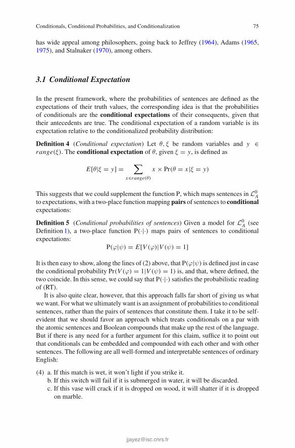
Conditionals, Conditional Probabilities, and Conditionalization 75
has wide appeal among philosophers, going back to Jeffrey (1964), Adams (1965,1975), and Stalnaker (1970), among others.
3.1 Conditional Expectation
In the present framework, where the probabilities of sentences are defined as theexpectations of their truth values, the corresponding idea is that the probabilitiesof conditionals are the conditional expectations of their consequents, given thattheir antecedents are true. The conditional expectation of a random variable is itsexpectation relative to the conditionalized probability distribution:
Definition 4 (Conditional expectation) Let θ, ξ be random variables and y ∈range(ξ). The conditional expectation of θ, given ξ = y, is defined as
E[θ|ξ = y] =∑
x∈range(θ)
x × Pr(θ = x |ξ = y)
This suggests that we could supplement the function P, which maps sentences in L0A
to expectations, with a two-place functionmapping pairs of sentences to conditionalexpectations:
Definition 5 (Conditional probabilities of sentences) Given a model for L0A (see
Definition1), a two-place function P(·|·) maps pairs of sentences to conditionalexpectations:
P(ϕ|ψ) = E[V (ϕ)|V (ψ) = 1]
It is then easy to show, along the lines of (2) above, that P(ϕ|ψ) is defined just in casethe conditional probability Pr(V (ϕ) = 1|V (ψ) = 1) is, and that, where defined, thetwo coincide. In this sense, we could say that P(·|·) satisfies the probabilistic readingof (RT).
It is also quite clear, however, that this approach falls far short of giving us whatwewant. For what we ultimately want is an assignment of probabilities to conditionalsentences, rather than the pairs of sentences that constitute them. I take it to be self-evident that we should favor an approach which treats conditionals on a par withthe atomic sentences and Boolean compounds that make up the rest of the language.But if there is any need for a further argument for this claim, suffice it to point outthat conditionals can be embedded and compounded with each other and with othersentences. The following are all well-formed and interpretable sentences of ordinaryEnglish:
(4) a. If this match is wet, it won’t light if you strike it.b. If this switch will fail if it is submerged in water, it will be discarded.c. If this vase will crack if it is dropped on wood, it will shatter if it is droppedon marble.
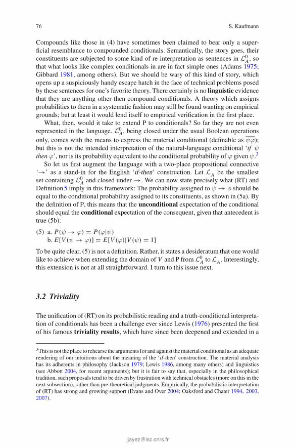
76 S. Kaufmann
Compounds like those in (4) have sometimes been claimed to bear only a super-ficial resemblance to compounded conditionals. Semantically, the story goes, theirconstituents are subjected to some kind of re-interpretation as sentences in L0
A, sothat what looks like complex conditionals in are in fact simple ones (Adams 1975;Gibbard 1981, among others). But we should be wary of this kind of story, whichopens up a suspiciously handy escape hatch in the face of technical problems posedby these sentences for one’s favorite theory. There certainly is no linguistic evidencethat they are anything other then compound conditionals. A theory which assignsprobabilities to them in a systematic fashion may still be found wanting on empiricalgrounds; but at least it would lend itself to empirical verification in the first place.
What, then, would it take to extend P to conditionals? So far they are not evenrepresented in the language. L0
A, being closed under the usual Boolean operationsonly, comes with the means to express the material conditional (definable as ψϕ);but this is not the intended interpretation of the natural-language conditional ‘if ψthen ϕ’, nor is its probability equivalent to the conditional probability of ϕ given ψ.3
So let us first augment the language with a two-place propositional connective‘→’ as a stand-in for the English ‘if-then’ construction. Let LA be the smallestset containing L0
A and closed under →. We can now state precisely what (RT) andDefinition5 imply in this framework: The probability assigned to ψ → φ should beequal to the conditional probability assigned to its constituents, as shown in (5a). Bythe definition of P, this means that the unconditional expectation of the conditionalshould equal the conditional expectation of the consequent, given that antecedent istrue (5b):
(5) a. P(ψ → ϕ) = P(ϕ|ψ)
b. E[V (ψ → ϕ)] = E[V (ϕ)|V (ψ) = 1]To be quite clear, (5) is not a definition. Rather, it states a desideratum that one wouldlike to achieve when extending the domain of V and P from L0
A to LA. Interestingly,this extension is not at all straightforward. I turn to this issue next.
3.2 Triviality
The unification of (RT) on its probabilistic reading and a truth-conditional interpreta-tion of conditionals has been a challenge ever since Lewis (1976) presented the firstof his famous triviality results, which have since been deepened and extended in a
3This is not the place to rehearse the arguments for and against thematerial conditional as an adequaterendering of our intuitions about the meaning of the ‘if-then’ construction. The material analysishas its adherents in philosophy (Jackson 1979; Lewis 1986, among many others) and linguistics(see Abbott 2004, for recent arguments); but it is fair to say that, especially in the philosophicaltradition, such proposals tend to be driven by frustration with technical obstacles (more on this in thenext subsection), rather than pre-theoretical judgments. Empirically, the probabilistic interpretationof (RT) has strong and growing support (Evans and Over 2004; Oaksford and Chater 1994, 2003,2007).

Conditionals, Conditional Probabilities, and Conditionalization 77
steady stream of subsequent work. Here I only summarize the first and simplest of theresults. It should be kept in mind, however, that many attempts to circumvent themwithin the general truth-conditional framework have been tried and shown to fail.
Suppose, then, that the probabilistic (RT) holds and conditionals denote proposi-tions in the usual sense—i.e., sets of worlds, or in the present framework, character-istic functions thereof. Then, since the denotations of conditionals are propositions,one can ask how their probabilities should be affected by conditionalization on otherpropositions: Technically, since V (ψ → ϕ) denotes a random variable, we should beable to derive its conditional expectation given that some arbitrary sentence is true.
Lewis (1976) was interested in the case that the conditioning sentence is ϕ, theconsequent of the conditional, or its negation. For those cases, Lewis made a pairof assumptions which seem rather plausible: First, given ϕ, the probability of theconditional ψ → ϕ should be 1; and second, given ϕ, it should be 0. Thus theequalities in (6) should hold.4
(6) a. P(ψ → ϕ|ϕ) = 1b. P(ψ → ϕ|ϕ) = 0
In the present framework, this amounts to the equalities in (7).
(7) a. E[V (ψ → ϕ)|V (ϕ) = 1] = 1b. E[V (ψ → ϕ)|V (ϕ) = 0] = 0
Now, since we are assuming that all sentences denote variables with range {0, 1} ,
this should hold for conditionals as well. But then (7) implies that with probability 1,the conditional is equivalent to its consequent! This consequence is grossly coun-terintuitive. As Lewis already pointed out, it implies that conditional consequentsare probabilistically independent of their antecedents, when in fact conditionals aretypically used to convey that they are not.
The literature on triviality that ensued after the publication of Lewis’s seminalargument is vast and varied, and this is not the place to do justice to its depth andbreadth. See Hájek and Hall (1994), Hájek (1994, 2012), Edgington (1995), Bennett(2003) and references therein for overviews, and Kaufmann (2005) for more discus-sion in the present framework. In the next section, I turn away from this literature ofmostly negative results to an approach which evades triviality.
4 Stalnaker Bernoulli Models
The challenge posed by the triviality results has proven to be formidable; but it is soonly under certain assumptionswhichLewis andmany subsequent authors either tookfor granted or found too valuable to give up. Specifically, the assumptions are that(i) the denotations of conditionals are propositions in the usual sense—here, sets of
4Lewis argued for the plausibility of (6) by invoking the Import-Export Principle, which in itsprobabilistic version requires that P(ψ → ϕ|χ) be equivalent to P(ϕ|ψχ). I avoid this move herebecause this principle is not universally accepted (see, for instance,Adams 1975; Kaufmann 2009).

78 S. Kaufmann
possible worlds (or their characteristic functions); and (ii) the values of conditionalsat individual worlds are fixed and do not depend on the probability distribution.Giving up these assumptions opens up an elegant way around the triviality results.This was first pointed out by van Fraassen (1976). Jeffrey (1991) arrived at a similarapproach (in spirit, if not in detail) from a different angle. The connection was madeexplicit by Stalnaker and Jeffrey (1994), which in turn inspired subsequent workincluding Kaufmann (2005, 2009).
4.1 Basic Idea
Themain innovation is a move from possible worlds to sequences of possible worldsas the entities at which sentences receive their truth values and which constitute thepoints in the probabilistic sample space. The idea was given a compelling intuitivemotivation by Stalnaker and Jeffrey (1994), with reference to Stalnaker’s (1968)similarity-based interpretation of conditionals.
Stalnaker’s proposal was that the truth value of ‘if A, then C’ at a possibleworld w is the truth value of its consequent C at a world “at which A is true andwhich otherwise differs minimally from the actual world.” What exactly such atheory predicts then depends on the notion of minimal difference. For instance, Stal-naker maintained that each world is maximally similar to itself; thus if A is trueat w, then no alternative world enters the evaluation because w is the most similarA-world to itself. Another assumption favored by Stalnaker was that for any worldw and proposition X (including the contradiction), there is a unique X -world that ismost similar to w. This assumption allowed Stalnaker to ensure that the conditionalhad certain logical properties which he considered desirable, especially ConditionalExcluded Middle, i.e., that for any pair A, C and world w, one of ‘if A, then C’ and‘if A, then not-C’ is true at w.
Now, the assumption that there is a uniquemost similar world for each propositionhas always been controversial.5 If we give it up, allowing formultiplemaximally sim-ilar worlds, but still insist on evaluating the conditional consequent relative to a singleantecedent-world, then the choice of world becomes essentially non-deterministic.Van Fraassen (1976) proposed a simple formal model of such a process: If we areat an antecedent-world, we are done choosing and evaluate the conditional by eval-uating its consequent. Otherwise, we continue to choose worlds in a sequence ofrandom trials (with replacement), where at each trial the probabilities that particularworlds will be chosen are determined by the original probability distribution. Thusthe probabilities at each trial are independent and identically distributed. Hence vanFraassen’s term “Stalnaker Bernoulli model,” suggestive of the special utility of thiskind of model in linking the intuitions behind Stalnaker’s possible-worlds semanticsfor conditionals to a standard probability-theoretic framework.
5See Lewis (1973), Stalnaker (1981) for some relevant arguments.

Conditionals, Conditional Probabilities, and Conditionalization 79
4.2 Implementation
Following van Fraassen (1976) I start with a probability model and define a productspace consisting of sets of denumerable sequences of possible worlds, along with aprobability measure that is derived from the original one. As before, sentences of thelanguage are mapped to (characteristic functions of) sets in the probability space;now these are sets of world sequences, rather than sets of worlds. The interpretationfunction is derived in the following way: Sentences in L0
A are evaluated at worldsequences in terms of the first world. Conditionalsψ → ϕ are evaluated at a sequenceby eliminating the (possibly empty) initial sub-sequence of worlds at which theantecedent is false, then evaluating the consequent at the remaining “tail” of thesequence. At sequences at which the antecedent is false throughout, the value isundefined. The details are given in the following definition.6
Definition 6 (Stalnaker Bernoulli model for LA) Let 〈Ω,F ,Pr, V 〉 be a probabilitymodel for L0
A. The corresponding Stalnaker Bernoulli model for LA is the tuple〈Ω∗,F∗,Pr∗, V ∗〉 such that:
• Ω∗ is the set of denumerable sequences of worlds in Ω .For ω∗ in Ω∗, I use the following notation:
– ω∗[n] is the nth world in ω∗ (thus ω∗[n] ∈ Ω)– ωn∗ is the tail of ω∗ starting at ω∗[n] (thus ωn∗ ∈ Ω∗)
• F∗ is the set of all products X1 × · · · × Xn × Ω∗, for n ≥ 1 and Xi ∈ F .• Pr∗ (·) is a probability measure on F∗ defined as follows, for Xi ∈ F :
Pr∗(X1 × · · · × Xn × Ω∗) = Pr(X1) × · · · × Pr(Xn)
• V ∗ maps pairs of sentences in LA and sequences in Ω∗ to values in {0, 1} asfollows, for ϕ,ψ ∈ LA:
if ϕ ∈ L0A, then V ∗(ϕ)(ω∗) = V (ϕ)(ω∗[1])
V ∗(ϕ)(ω∗) = 1 − V ∗(ϕ)(ω∗)V ∗(ϕψ)(ω∗) = V ∗(ϕ)(ω∗) × V ∗(ψ)(ω∗)
V ∗(ϕ → ψ)(ω∗) = V ∗(ψ)(ωn∗)for the least n s.t. V ∗(ϕ)(ωn∗) = 1
6In van Fraassen’s original version, a conditional is true, rather than undefined, at a sequence notcontaining any tails at which the antecedent is true. The difference is of no consequence for thecases I discuss here. In general, I find the undefinedness of the conditional probability in suchcases intuitively plausible and preferable, as it squares well with widely shared intuition (in thelinguistic literature, at least) that indicative conditionals with impossible antecedents give rise topresupposition failure. Moreover, it follows from the results below that the (un)definedness is fairlywell-behaved, in the sense that the value of the conditional is defined with probability zero or one,according as the probability of the antecedent is zero or non-zero.
80 S. Kaufmann
I use boldfaced letters like ‘X, Y’ to refer to elements in F∗. Notice that even ifF is the powerset of Ω , F∗ is a not the powerset of Ω∗, but a proper subset of thelatter. For instance, consider two arbitrary worlds ω1,ω2 and two arbitrary sequencesω∗
a = 〈ω1,ω2, . . .〉 and ω∗b = 〈ω2,ω1, . . .〉. The set
{ω∗
a ,ω∗b
}is in the powerset of
Ω∗ but not in F∗, although it is a subset of sets in F∗. This is not a deficiency forthe purposes that I am putting this model to, since the truth conditions do not allowfor the case that, say, a sentence is true at all and only the sequences in {ω∗
a ,ω∗b}.
As before, the probabilities assigned to sentences are the expectations of theirtruth values. Recall that sentences containing conditionals differ from sentences inL0
A in that their values are not guaranteed to be defined: If a given sequence does notcontain any A-worlds, then the value of any conditional with antecedent A at thatsequence is undefined, and so is the value of compounds containing the conditionalin question. The assignment of probabilities to sentences therefore comes with aqualification:
Definition 7 (Probabilities of sentences) Given a Stalnaker Bernoulli model for LA(see Definition6), a function P∗ maps sentences to real numbers as follows:
P∗(ϕ) = E∗[V ∗(ϕ)|V ∗(ϕ) ∈ {0, 1}]
The conditioning event on the right-hand side in this definition is that the value ofthe sentence in question is defined. It turns out that this is not a very constrainingcondition, as the following outline of an argument shows (see also van Fraassen1976; Kaufmann 2009).
First, from the definition of V ∗ it follows immediately that the values of sen-tences in L0
A—i.e., sentences not containing any occurrences of the conditionalconnective—are defined at all sequences. Consider next a “first-order” conditional—that is, a sentence of the form ϕ → ψ, where both ϕ and ψ are in L0
A. There is onlyone reason why the value of this sentence at a sequence ω∗ could be undefined,namely that its antecedent ϕ is false throughout ω∗ (i.e., at ω∗[n] for all n). Propo-sition1 establishes that whenever the antecedent has positive probability, the set ofsequences with this property has probability 0. (Proofs of this and all subsequentresults are given in the Appendix.)
Proposition 1 (van Fraassen 1976) For X ∈ F , if Pr(X) > 0, then Pr∗(⋃
n∈N(X
n × X × Ω∗))
= 1.
As an immediate consequence, the value of the conditional is almost surely definedwhen its antecedent has positive probability. By similar reasoning, the value of theconditional is almost surely undefined if the antecedent has zero probability.7
As it stands, Proposition1 only applies to elements of F , i.e., denotations ofsentences in L0
A. It can be generalized to other sets, in particular the denotations of
7In probability theory, an event happens “almost surely” if its probability is 1. This notion shouldnot be confused with logical necessity.

Conditionals, Conditional Probabilities, and Conditionalization 81
conditionals, but I will not pursue this argument here because the points I aim tomake in this paper can be made with reference to simple sentences.
Henceforth, to forestall any complexities of exposition arising from the possibil-ity of undefinedness, I will implicitly limit the discussion to sentences, all of whoseconstituents have positive probability. With this assumption, their values are guaran-teed to be defined almost surely, thus the conditioning event on the right-hand sideof the equation in Definition7 can be ignored.
Van Fraassen (1976) proved the following “Fraction Lemma” (credited to IanHacking), which turns out to be useful in calculating the probabilities of both simpleand compounded conditionals.
Lemma 1 (van Fraassen 1976) If Pr(X) > 0, then∑
n∈N Pr(X
)n = 1/Pr(X).
As a straightforward consequence of the foregoing results, it is easy to ascertainthat the probabilities of first-order conditionals are the corresponding conditionalprobabilities.
Theorem 1 (van Fraassen 1976) For A, C ∈ L0A, if P(A) > 0, then P∗ (A → C) =
P(C |A).
In addition, it is easy to see that for all ϕ ∈ L0A, P
∗(ϕ) = P(ϕ). Specifically, this istrue for AC and A. Thus as an immediate corollary of Theorem1, we have that
(8) P∗(A → C) = P∗(C |A)
This is why the interpretation in a Stalnaker Bernoulli model is not subject to theLewis-style triviality results: The denotation of the conditional is both a proposition(specifically, the characteristic function of a set of sequences) and the correspondingconditional expectation.
Theorem1 illustrates the simplest case of a correspondence between the prob-abilities assigned to conditional sentences in a Stalnaker Bernoulli model and theprobabilities that their L0
A-constituents receive in the original probability model.Similar calculations, albeit of increasing complexity, can be carried out for sen-tences of arbitrary complexity. This was hinted at by Stalnaker and Jeffrey (1994)and worked out for cases of conditional antecedents and consequents by Kaufmann(2009). The formulas in (9a) through (9d) serve as illustration; for more details andproofs, the reader is invited to consult Kaufmann (2009).
(9) For all A, B, C, D in L0A:
a. If P(A) > 0 and P(C) > 0, thenP∗((A → B) ∧ (C → D))
= P(ABC D) + P(D|C) + P(ABC) + P(B|A)P(C D A)
P(A ∨ C)b. If P(A) > 0,P(C) > 0, and P(B|A) > 0, then
P∗((A → B) → (C → D))
= P(ABC D) + P(D|C)P(ABC) + P(B|A)P(AC D)
P(A ∨ C)P(B|A)

82 S. Kaufmann
c. If P(B) > 0 and P(C) > 0, thenP∗(B → (C → D)) = P(C D|B) + P(D|C)P(C |B)
d. If P(A) > 0 and P(B|A) > 0, thenP∗((A → B) → D) = P(D|AB)P(A) + P(D A)
More complex compounds also receive probabilities under this approach, but theyare beyond the scope of this paper because it is not clear what the empirical situationis in those cases.
4.3 Back to Probability Models
The preceding subsection showed how to start from an ordinary probability modeland obtain values and probabilities for sentences in the derived Stalnaker Bernoullimodel, defined by V ∗ and Pr∗. Now Stalnaker and Jeffrey (1994) (and, followingthem, Kaufmann 2009) did not stop there, for their ultimate goal was to interpret sen-tences inLA in the original probability model—i.e., to extend the value assignmentfunction V from L0
A to LA.Intuitively, the idea is to let V (ϕ)(ω) be the conditional expectation of V ∗(ϕ),
given the set of sequences in Ω∗ whose first world is ω∗ –that is, the set{ω∗ ∈ Ω∗|ω∗[1] = ω} . But this set may well have zero probability, since its prob-ability is defined as Pr({ω}). Stalnaker and Jeffrey’s workaround is to define theexpectation relative to the ω∗-subspace of Ω∗, obtained by effectively “ignoring”the first position of the sequences.
Definition 8 Given a probability model M = 〈Ω,F ,Pr, V 〉 for L0A, the interpre-
tation function is extended to LA as follows: For all ϕ ∈ LA and ω ∈ Ω ,
V (ϕ)(ω) = Pr∗({
ω2∗∣∣∣ω∗[1] = ω and V ∗(ϕ)(ω∗) = 1
})
where E∗,V ∗ are defined relative to the Stalnaker Bernoulli model based on M.
It is then possible to calculate, for sentences in LA, the values they receive under V .The simple case of first-order conditionals is given in (10).
(10) V (A → C)(ω) =
⎧⎪⎨
⎪⎩
1 if V (A)(ω) = V (C)(ω) = 1
0 if V (A)(ω) = 1, V (C)(ω) = 0
P(C |A) if V (A) = 0
The first two cases on the right-hand-side of (10) are straightforward: The value ofV ∗(A → C) is true at either all or none of the sequences starting with an A-world,depending on the value ofC at the first world. The third case is obtained by observingthat the set of sequences starting with a A-world at which the conditional is true is theunion of all sets of sequences consisting of n A-worlds followed by an AC-world, for
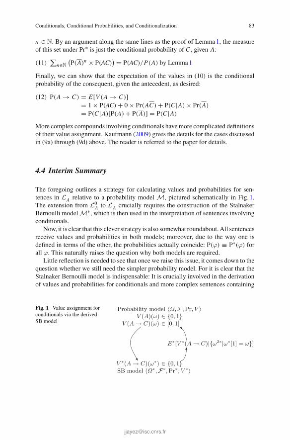
Conditionals, Conditional Probabilities, and Conditionalization 83
n ∈ N. By an argument along the same lines as the proof of Lemma1, the measureof this set under Pr∗ is just the conditional probability of C , given A:
(11)∑
n∈N(P(A)n × P(AC)
) = P(AC)/P(A) by Lemma1
Finally, we can show that the expectation of the values in (10) is the conditionalprobability of the consequent, given the antecedent, as desired:
(12) P(A → C) = E[V (A → C)]= 1 × P(AC) + 0 × Pr(AC) + P(C |A) × Pr(A)
= P(C |A)[P(A) + P(A)] = P(C |A)
More complex compounds involving conditionals havemore complicated definitionsof their value assignment. Kaufmann (2009) gives the details for the cases discussedin (9a) through (9d) above. The reader is referred to the paper for details.
4.4 Interim Summary
The foregoing outlines a strategy for calculating values and probabilities for sen-tences in LA relative to a probability model M, pictured schematically in Fig. 1.The extension from L0
A to LA crucially requires the construction of the StalnakerBernoulli modelM∗, which is then used in the interpretation of sentences involvingconditionals.
Now, it is clear that this clever strategy is also somewhat roundabout. All sentencesreceive values and probabilities in both models; moreover, due to the way one isdefined in terms of the other, the probabilities actually coincide: P(ϕ) ≡ P∗(ϕ) forall ϕ. This naturally raises the question why both models are required.
Little reflection is needed to see that once we raise this issue, it comes down to thequestion whether we still need the simpler probability model. For it is clear that theStalnaker Bernoulli model is indispensable: It is crucially involved in the derivationof values and probabilities for conditionals and more complex sentences containing
Fig. 1 Value assignment forconditionals via the derivedSB model
Probability model 〈Ω, F ,Pr, V 〉V (A)(ω) ∈ {0, 1}
V (A → C)(ω) ∈ [0, 1]
E∗[V ∗(A → C)|{ω2∗|ω∗[1] = ω}]
V ∗(A → C)(ω∗) ∈ {0, 1}SB model 〈Ω∗, F∗,Pr∗, V ∗〉
84 S. Kaufmann
conditional constituents.8 But then,what is the utility of having the traditional, world-based model?
I will not venture to offer a conclusive answer to this question at this point;surely one factor in favor of the conventional possible-worlds model is its familiarityand relatively straightforward and well-understood interface with general topics inepistemology and metaphysics. So the question is to what extent these connectionscould be recreated in a framework thatwas primarily based on the Stalnaker Bernoulliapproach.
Aside from such big-picture considerations, it isworth stressing that a general shiftto the Stalnaker Bernoulli framework would bring additional functionality beyondthe extension of the interpretation to LA. To wit, adopting the approach of assigningintermediate values to conditionals at worlds at which their antecedents are false,we face the problem that it there is no general rule of conditionalization involvingconditionals—either for conditioning their denotations on other events, or for condi-tioning other events on them. This problem does not arise in the Stalnaker Bernoulliapproach, where the probability of a conditional is the probability of a proposition(in addition to being a conditional probability).
To get such a project off the ground, however, much work has to be done. Forone thing, the Stalnaker Bernoulli model would need some intuitive interpretation.Moreover, we would need plausible representations of such elementary notions asbelief change by conditionalization.
Regarding the first of these desiderata—an intuitive interpretation of StalnakerBernoulli models—we can derive some inspiration from the suggestions of Stal-naker and Jeffrey, cited above. A set X of world sequences represents two kinds ofinformation: “factual” beliefs are encoded in the set of “firstworlds” {ω∗[1]|ω∗ ∈ X},which is where all sentences inL0
A receive their truth values. The other kind of infor-mation consists in “conditional” beliefs, encoded in the sequences
{ω2∗∣∣ω∗ ∈ X
}.
Each sequence represents a possible outcome of a countable sequence of randomchoices of a world (with replacement), modeling a non-deterministic variant of theinterpretation of conditionals in terms of a Stalnaker selection function.9
With this in mind, I will set the first issue aside and spend the rest of this paperfocusing on the second issue, the definition of belief update by conditionalization ina Stalnaker Bernoulli model.
8As a historical side note, it is worth pointing out that some of the functionality delivered hereby the Stalnaker Bernoulli model can also be achieved in a simpler model. This was shown byJeffrey (1991), who developed the random-variable approach with intermediate truth values withoutrelying on van Fraassen’s construction. But that approach has its limits, for instancewhen it comes toconditionals with conditional antecedents, and can be seen as superseded by the Stalnaker Bernoulliapproach.9In a related sense, onemay also think of a given set of sequences as representing all paths followingan introspective (i.e., transitive and euclidean) doxastic accessibility relation. I leave the furtherexploration of this connection for future work.

Conditionals, Conditional Probabilities, and Conditionalization 85
M1 = 〈Ω, F ,Pr1, V1〉V1(ϕ)(ω) ∈ {0, 1}, ϕ ∈ L0
A
V1(ϕ)(ω) ∈ [0, 1] in general
M2 = 〈Ω, F ,Pr2, V2〉V2(ϕ) ≡ V1(ϕ), ϕ ∈ L0
A
V2(ϕ) �≡ V1(ϕ) in general
M∗1 = 〈Ω∗, F∗,Pr∗1, V ∗〉
V ∗(ϕ)(ω∗) ∈ {0, 1}M∗
2 = 〈Ω∗, F∗,Pr∗2, V ∗〉V ∗(ϕ)(ω∗) ∈ {0, 1}
conditioning on ϕ ∈ L0A
conditioning in general:not defined
???
Fig. 2 Belief update in probability models with SB interpretations for conditionals
5 Conditionalization
What is the problem with conditionalization in Stalnaker Bernoulli models? Figure2gives a general overview. Suppose we start out, as we did in this paper, with M1,a conventional probabilistic possible-worlds model. In it, the non-conditional sen-tences inL0
A receive truth values atworlds, but in order to extend the value assignmentto conditionals in accordance with the probabilistic interpretation of (RT), we takea detour via the derived Stalnaker Bernoulli model M∗
1 (as shown in Fig. 1). Thisallows us to extend V1 to conditionals.
Now, suppose we want to update the belief model by conditioning on a new pieceof information, say, that some sentence ϕ is true. If ϕ ∈ L0
A, this is not a problem:As usual in Bayesian update, we conditionalize by shifting the probability mass tothe set of worlds at which ϕ is true, then renormalize the measure so as to ensurethat we have once again a probability distribution, thus obtaining Pr2.
Now, a number of things are noteworthy about this update operation. First, alongwith the shift from Pr1 to Pr2, the value assignment for conditionals must also changein order to ensure that the expectation of the new measure is the conditional proba-bility. Thus we obtain a valuation function V2 which agrees with V1 on all sentencesinL0
A, but may differ in the values it assigns to conditionals and sentences containingthem. The second noteworthy point about the update is that we have no systematicway of deriving this new assignment function V2 from V1. After the update, the newvalues for conditionals have to be filled in by once again taking the detour via thederived Stalnaker Bernoulli model, now M∗
2. Thirdly, while the update with a sen-tence in L0
A just discussed merely presents a minor inconvenience (in calling for arecalculation of the values of sentences not inL0
A via the derived Stalnaker Bernoullimodel), matters are worse if the incoming information is conditional, i.e., the infor-mation that some sentence not in L0
A is true. Whenever such a sentence takes valuesstrictly less than 1, we do not have a way to conditionalize on it.
Notice, though, that these problems would not arise if we were using StalnakerBernoulli models throughout. InM∗
1 andM∗2, all sentences receive values in {0, 1}
almost surely (with the above caveats about the possibility of undefinedness andits intuitive justification). Moreover, notice that the two Stalnaker Bernoulli modelsshare the same valuation function. For recall that V ∗(ϕ)(ω∗) only depends on the

86 S. Kaufmann
structure of ω∗, not on the probability distribution. And since conditionals denotepropositions in these models (i.e., elements of F∗), conditionalization involvingthose denotations can proceed in the familiar fashion. I take all of these facts to becompelling arguments in favor of the exclusive use of Stalnaker Bernoulli models.
5.1 Shallow Conditioning
How exactly should belief update be carried out in Stalnaker Bernoulli models? Tosee why this is an issue, consider what would seem to be the most straightforwardway to define conditionalization on a sentenceϕ inM∗
1. Presumably, similarly to theanalogous procedure on M1, this would involve shifting the probability mass ontosequences at which V ∗(ϕ) evaluates to 1, then renormalizing the measure to ensurethat the result is again a probability distribution.10
Now, the problem with this approach is that the resulting probability distributionis not Pr∗2, hence the resulting model is notM∗
2. It is easy to see why this is the case.For concreteness, let us assume that the new information is that some sentence Ain L0
A is true. By the definition of the Stalnaker Bernoulli model, V ∗(A)(ω∗) = 1whenever V (A)(ω∗[1]) = 1—in words, if the first world in ω∗ is an A-world. Thisincludes all sequences which begin with an A-world, regardless of what happenslater on in them.
But this is not the set of sequences over which the probability is distributedin M∗
2. For recall that M∗2 was obtained from M1 by conditionalization on the
information that A is true. As a result of this operation, inM2 the entire probabilitymass is assigned to worlds at which A is true. Hence, in M∗
2, the probability massis concentrated on sequences which consist entirely of A-worlds (i.e., sequences ω∗such that V ∗(A)(ωn∗) = 1 for all n).
Thus in order to fill in the missing step fromM∗1 toM∗
2 in Fig. 2, we would haveto conditionalize on the set of sequences in (13b), rather than (13a).
(13) a. {ω∗ ∈ Ω∗|V ∗(ϕ)(ω∗) = 1}b. {ω∗ ∈ Ω∗|V ∗(ϕ)(ωn∗) = 1 for all n ≥ 1}
However, the set in (13b) has zero probability whenever the probability of ϕ isless than 1. Indeed, for any X ∈ F , the set X∗ of sequences consisting entirely ofX -worlds has probability 1 or 0, according as the probability of X is 1 or less than 1:
(14) Pr∗(X∗) = limn→∞ Pr(X)n ={1 if Pr(X) = 1
0 otherwise
Clearly a different definition is needed to work around this problem.
10An alternative way of achieving the same result would be to model belief update in terms of“truncation” of world sequences along the lines of the interpretation of conditionals, chopping offinitial sub-sequences until the remaining tail verifiesϕ. I will not go into the details of this operationhere; it corresponds to the operation of shallow conditioning discussed in this subsection, for thesame reason that the probabilities of conditionals equal the corresponding conditional probabilities.
Conditionals, Conditional Probabilities, and Conditionalization 87
5.2 Deep Conditioning
It is not uncommon in discussions of probability to see “Bayes’s Rule” as a definitionof conditional probability:
(BR) Pr(X |Y ) = Pr(X ∩ Y )
Pr(Y )when Pr(Y ) > 0
Taken as a definition, this suggests that the conditional probability is generally unde-fined when the probability of the conditioning event is 0. But this view has manyproblematic consequences, not the least of them being that it predicts that the condi-tional probability is undefined in cases in which we in fact have clear intuitions thatit exists and what it should be.11 This point has been discussed in the philosophicalliterature (see for instance Stalnaker and Jeffrey 1994; Jeffrey 2004; Hájek 2003,2011, and references therein), but the misconception that (BR) is the definition ofconditional probability is apparently hard to root out.12
My own take on conditional probability follows the lead of Stalnaker and Jeffrey(1994) and Jeffrey (2004): (BR) is not a definition, but a restatement of the “ProductRule” (PR):
(PR) Pr(X |Y ) × Pr(Y ) = P(X ∩ Y )
Most crucially, (PR) should not be mistaken for a definition either, but as an axiomregulating the relationship between unconditional and conditional probabilitieswhenboth are defined.
Following this general strategy, in Definition9 I give one definition of a two-placefunction Pr∗ (·|·) , then I proceed to show that it is in fact properly called a conditionalprobability.
Definition 9 (Stalnaker Bernoulli model with conditional probability)An Stalnaker Bernoulli model with conditional probability is a tuple〈Ω∗,F∗,Pr∗ (·) ,Pr∗ (·|·) , V ∗〉, where 〈Ω∗,F∗,Pr∗ (·) , V ∗〉 is a StalnakerBernoulli model (see Definition6) and Pr∗ (·|·) is a partial function mapping pairsof propositions in F∗ to real numbers as follows, for all X, Y in F∗:
Pr∗ (X|Y) = limn→∞
Pr∗ (X1 ∩ Y1 × · · · × Xn ∩ Yn × Ω∗)Pr∗ (Y1 × · · · × Yn × Ω∗)
11As a simple example, consider the task of choosing a point (x, y) at random from a plane. Fixsome point (x∗, y∗) and consider the conditional probability that y > y∗, given x = x∗ (intuitively,the conditional probability that the randomly chosen point will lie above (x∗, y∗), given that it lieson the vertical line through (x∗, y∗)).We have clear intuitions as to what this conditional probabilityis and how it depends on the location of the cutoff point x∗; but the probability that the randomlychosen point lies on the line is 0.12Notice, incidentally, that the view on conditional probability just endorsed is not at odds with theremarks on the undefinedness of the values of conditionals at world sequences throughout whichthe antecedent is false (see footnote 6). For one thing, technically the undefinedness discussedthere does not enter the picture because some conditional probability is undefined. But that aside,I emphasize that I do not mean to claim that conditional probabilities given zero-probability eventsare always defined, only that they can be.
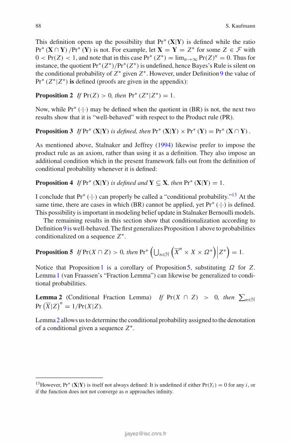
88 S. Kaufmann
This definition opens up the possibility that Pr∗ (X|Y) is defined while the ratioPr∗ (X ∩ Y) /Pr∗ (Y) is not. For example, let X = Y = Z∗ for some Z ∈ F with0 < Pr(Z) < 1, and note that in this case Pr∗ (Z∗) = limn→∞ Pr(Z)n = 0. Thus forinstance, the quotient Pr∗(Z∗)/Pr∗(Z∗) is undefined, hence Bayes’s Rule is silent onthe conditional probability of Z∗ given Z∗. However, under Definition9 the value ofPr∗ (Z∗|Z∗) is defined (proofs are given in the appendix):
Proposition 2 If Pr(Z) > 0, then Pr∗ (Z∗|Z∗) = 1.
Now, while Pr∗ (·|·) may be defined when the quotient in (BR) is not, the next tworesults show that it is “well-behaved” with respect to the Product rule (PR).
Proposition 3 If Pr∗ (X|Y) is defined, then Pr∗ (X|Y) × Pr∗ (Y) = Pr∗ (X ∩ Y) .
As mentioned above, Stalnaker and Jeffrey (1994) likewise prefer to impose theproduct rule as an axiom, rather than using it as a definition. They also impose anadditional condition which in the present framework falls out from the definition ofconditional probability whenever it is defined:
Proposition 4 If Pr∗ (X|Y) is defined and Y ⊆ X, then Pr∗ (X|Y) = 1.
I conclude that Pr∗ (·|·) can properly be called a “conditional probability.”13 At thesame time, there are cases in which (BR) cannot be applied, yet Pr∗ (·|·) is defined.This possibility is important inmodeling belief update in Stalnaker Bernoulli models.
The remaining results in this section show that conditionalization according toDefinition9 iswell-behaved. Thefirst generalizes Proposition1 above to probabilitiesconditionalized on a sequence Z∗.
Proposition 5 If Pr(X ∩ Z) > 0, then Pr∗(⋃
n∈N(
Xn × X × Ω∗
)∣∣∣Z∗)
= 1.
Notice that Proposition1 is a corollary of Proposition5, substituting Ω for Z .Lemma1 (van Fraassen’s “Fraction Lemma”) can likewise be generalized to condi-tional probabilities.
Lemma 2 (Conditional Fraction Lemma) If Pr(X ∩ Z) > 0, then∑
n∈NPr
(X |Z)n = 1/Pr(X |Z).
Lemma2allowsus to determine the conditional probability assigned to the denotationof a conditional given a sequence Z∗.
13However, Pr∗ (X|Y) is itself not always defined: It is undefined if either Pr(Yi ) = 0 for any i , orif the function does not not converge as n approaches infinity.

Conditionals, Conditional Probabilities, and Conditionalization 89
6 Some Consequences for Conditionals
To sum up the preceding subsections, the Stalnaker Bernoulli framework offers twonatural ways to interpret conditionals: by the rule in Definition6, and by deep condi-tioning. The two are distinguished by the characterization of the conditioning event,i.e., the way in which the incoming information is used in singling out the set ofsequences on which to concentrate the probability mass. For a given sentence ϕ, thetwo options are repeated in (17). I argued above that deep conditioning is what isrequired to model belief update by conditionalization.
(17) a. {ω∗ ∈ Ω∗|V ∗(ϕ)(ω∗) = 1} [shallow]b. {ω∗ ∈ Ω∗|V ∗(ϕ)(ωn∗) = 1 for all n} [deep]
In addition, I believe it is likely that both update operations are required to model theinterpretation of conditionals. To see this, consider first what the difference comesdown to in terms of the intuitive interpretation of the two versions of update.
Recall first the intuitive interpretation of a Stalnaker Bernoulli model as a repre-sentation of epistemic states. The idea was that a world sequence represents factualinformation in the first world, and conditional information in the tail following thefirst world. As already mentioned in footnote 9, from the modal-logic perspectiveon the representation of knowledge and belief, one can alternatively think of thesequences as representing all possible paths along an introspective doxastic accessi-bility relation. This intuitive interpretation of world sequences corresponds well withthe proposal to model belief update by conditionalization on the set of sequencesthroughout which the incoming sentence is true (as opposed to the set of sequencesat which the sentence evaluates to 1).
With all this in mind, I believe that we can discern in the distinction between shal-low and deep conditioning an intuitively real difference in ways to “hypotheticallyadd,” in Ramsey’s words, a sentence ϕ to one’s probabilistic “stock of knowledge”:Shallow update consists in assuming that ϕ is true, whereas deep udpate consists inassuming that ϕ is learned.
The distinction between these two modes of update underlies certain problematicexamples which have been discussed widely in the literature on conditionals. Amongthem are simple conditionals like (18a), attributed to Richmond Thomason by vanFraassen (1980), and (18b) from Lewis (1986).
(18) a. If my wife deceives me, I won’t believe it.b. If Reagan works for the KGB, I’ll never believe it.
In both cases, the conditional antecedent is intuitively not correctly paraphrased byany variant of the locution ‘If I know/learn that’ . . ., for otherwise it would not makesense togetherwith the consequent. Yet these examples are perfectlywell-formed andinterpretable. What the examples show is that it is possible for speakers to supposethat something is the case unbeknownst to them. The present framework opens up away to model the difference in a probabilistic setting.

90 S. Kaufmann
Another difference between the two modes of update concerns the interpretationof right-nested conditionals, i.e., sentences of the form B → (C → D). Here we seea tangible consequence of the fact that the update with the antecedent B determinesthe context for the interpretation of the consequent C → D. Theorem2 states thegeneral result for deep conditioning with sentences of this form.
Theorem 2 If P (BC) > 0, then P∗ (C → D|B∗) = P (D|BC).
Theorem1 is a special case of Theorem2, again obtained by substituting the tautologyfor B.
What is notable about this result is that it resembles the Conditional Import-Export Principle, i.e., the rule that the conditional probability of ϕ → ψ given χshould equal the conditional probability of ψ given ϕχ. Theorem2 shows that theImport-Export Principle holds for right-nested conditionals under deep conditioningon the antecedent. On the other hand, it does not hold under the standard StalnakerBernoulli interpretation. Recall from (9c) above that the expectation of the valuesassigned to such right-nested conditionals is quite different:
(9c) If P(B) > 0 and P(C) > 0, thenP∗(B → (C → D)) = P(C D|B) + P(D|C)P(C |B)
There is much room for further explorations into the ramifications of this distinction,for right-nested conditionals as well as for the others listed in (9b) and (9d) above.These investigations are left to future work.
7 Conclusions
I have argued that it makes good sense to investigate the utility of Stalnaker Bernoullimodels as a formal tool for the representation and analysis of belief states and theirdynamics. The main arguments in favor of such a move draw on the viability ofan account long these lines that is immune to Lewisian triviality results. But I alsoshowed that once we start to investigate the matter seriously, a number of additionalsubtleties and advantages come into view which merit further study. The differencebetween shallowanddeep conditioning and its potential applications in the analysis ofcounterexamples to the Import-Export Principlewas one such example. Additionally,the framework promises to offer a straightforward account of belief updates involvingconditionals, whose theoretical implementation and empirical verification remain tobe carried out. And all of this, in a sense, leads up to the big question: whether itis time to do away with the time-honored but simplistic possible-worlds models, ifonly to get the probabilities of conditionals right.

Conditionals, Conditional Probabilities, and Conditionalization 91
Appendix: Proofs
Proposition 1 For X ∈ F , if Pr(X) > 0, then Pr∗(⋃
n∈N(
Xn × X × Ω∗
))= 1.
Proof Notice that⋃
n∈N(
Xn × X × Ω∗
)is the set of all sequences containing at
least one X -world, thus its complement is X∗. Now
Pr∗(⋃
n∈N(
Xn × X × Ω∗
))= 1 − Pr∗
(X
∗)
= 1 − limn→∞ Pr∗(
Xn × Ω∗
)= 1 − limn→∞ Pr
(X
)n = 1 since Pr(X) < 1. �
Lemma 1 If Pr(X) > 0, then∑
n∈N Pr(X
)n = 1/Pr(X).
Proof∑
n∈N Pr(X
)n × Pr (X) = ∑n∈N
(Pr
(X
)n × Pr (X))
= ∑n∈N Pr∗
(X
n × X × Ω∗)
= Pr∗(⋃
n∈N(
Xn × X × Ω∗
))= 1 by Proposi-
tion1. �
Theorem 1 For A, C ∈ L0A, if P(A) > 0, then P∗ (A → C) = P(C |A).
Proof By Definition6, the set of sequences ω∗ such that V ∗(A → C)(ω∗) =1 is the union
⋃n∈N
({ω ∈ Ω|V (A)(ω) = 0}n × {ω ∈ Ω|V (AC)(ω) = 1} × Ω∗).Since the sets for different values of n are mutually disjoint, the probability of theunion is the sum of the probabilities for all n. Now, for all X, Y ∈ F ,
Pr∗(⋃
n∈N(
Yn × (X ∩ Y ) × Ω∗
))= ∑
n∈N Pr∗(
Yn × (X ∩ Y ) × Ω∗
)
= ∑n∈N
(Pr
(Y
)n × Pr(X ∩ Y ))
= ∑n∈N Pr
(Y
)n × Pr(X ∩ Y )
= Pr(X ∩ Y )/Pr(Y ) by Lemma1.In particular, let X, Y be the set of worlds in Ω at which V (C) and V (A) are true,respectively. �
Proposition 2 If Pr(Z) > 0, then Pr∗ (Z∗|Z∗) = 1.
Proof Pr∗ (Z∗|Z∗) = limn→∞ Pr∗ (Zn × Ω∗|Zn × Ω∗) = 1. �
Proposition 3 If Pr∗ (X|Y) is defined, then Pr∗ (X|Y) × Pr∗ (Y) = Pr∗ (X ∩ Y) .
Proof Since Pr∗ (X|Y) is defined, Pr(Yn) > 0 for all n. Thus Pr∗ (X|Y) × Pr∗ (Y)
= limn→∞Pr∗
(X1 ∩ Y1 × · · · × Xn ∩ Yn × Ω∗)
Pr∗ (Y1 × · · · × Yn × Ω∗)× limn→∞ Pr∗
(Y1 × · · · × Yn × Ω∗)
= limn→∞(Pr∗ (X1 ∩ Y1 × · · · × Xn ∩ Yn × Ω∗)
Pr∗ (Y1 × · · · × Yn × Ω∗)× Pr∗ (Y1 × · · · × Yn × Ω∗)
)
= limn→∞ Pr∗ (X1 ∩ Y1 × · · · × Xn ∩ Yn × Ω∗) = Pr∗ (X ∩ Y) �
Proposition 4 If Pr∗ (X|Y) is defined and Y ⊆ X, then Pr∗ (X|Y) = 1.

92 S. Kaufmann
Proof For all i ≥ 1, Xi ∩ Yi = Yi since Y ⊆ X, and Pr(Yi ) > 0 since Pr∗ (X|Y) is
defined. Thus Pr∗ (X|Y) = limn→∞Pr∗ (Y1 × · · · × Yn × Ω∗)Pr∗ (Y1 × · · · × Yn × Ω∗)
= 1. �
The following auxiliary result will be useful in the subsequent proofs.
Proposition 9 If Pr(Z) > 0, then for Xi ∈ F and n ∈ N,
Pr∗(X1 × · · · × Xn × Ω∗∣∣Z∗) = Pr∗
(X1 × · · · × Xn × Ω∗∣∣Zn × Ω∗)
Proof Immediate because Z ⊆ Ω . �
The significance of Proposition 9 derives from the fact that the sets of sequences atwhich a given sentence in LA is true can be constructed (using set operations underwhich F∗ is closed) out of sequence sets ending in Ω∗. This is obvious for the non-conditional sentences in L0
A. For conditionals ϕ → ψ the relevant set is the union ofsets of sequences consisting of n ϕ-worlds followed by a ϕψ-world. For each n, thecorresponding set ends in Ω∗ and therefore can be conditioned upon Z∗ as shownin Proposition 9. Since these sets for different numbers n are mutually disjoint, theprobability of their union is just the sum of their individual probabilities.
Proposition 5 If Pr(X ∩ Z) > 0, then Pr∗(⋃
n∈N(
Xn × X × Ω∗
)∣∣∣Z∗)
= 1.
Proof Since Pr(X ∩ Z) > 0, Pr(X ∩ Z) < Pr(Z). Thus
Pr∗(⋃
n∈N(
Xn × X × Ω∗
)∣∣∣Z∗)
= 1 − Pr∗(
X∗∣∣∣Z∗
)
= 1 − limn→∞Pr∗
((X ∩ Z)n × Ω∗)
Pr∗ (Zn × Ω∗)= 1 − limn→∞
Pr(X ∩ Z
)n
Pr (Z)n
= 1 − limn→∞
(Pr
(X ∩ Z
)
Pr (Z)
)n
= 1 since Pr∗(X ∩ Z) < Pr∗(Z) �
Lemma 2 If Pr(X ∩ Z) > 0, then∑
n∈N Pr(X |Z)n = 1/Pr(X |Z).
Proof Since Pr(X ∩ Z) = Pr(Z) × Pr(X |Z), both Pr(Z) > 0 and Pr(X |Z) > 0.∑
n∈N Pr(X |Z)n × Pr (X |Z) = ∑
n∈N(Pr
(X |Z)n × Pr (X |Z)
)
= ∑n∈N
Pr(X ∩ Z
)n × Pr (X ∩ Z)
Pr (Z)n+1 = ∑n∈N
Pr∗((X ∩ Z)n × (X ∩ Z) × Ω∗)
Pr∗(Zn+1 × Ω∗)
= ∑n∈N Pr∗
(X
n × X × Ω∗∣∣∣Zn+1 × Ω∗
)
= ∑n∈N Pr∗
(X
n × X × Ω∗∣∣∣Z∗
)by Proposition9
= Pr∗(⋃
n∈N(
Xn × X × Ω∗
)∣∣∣Z∗)
= 1 by Proposition5. �
Theorem 2 If P (BC) > 0, then P∗ (C → D|B∗) = P (D|BC).
Conditionals, Conditional Probabilities, and Conditionalization 93
Proof P∗ (C → D|B∗) = limn→∞P∗(((C → D) ∧ B)n × Ω∗)
P∗ (Bn × Ω∗)
= limn→∞∑n−1
i=0 P(C B)i × P(C DB)
P(B)n
= limn→∞∑n−1
i=0 P(C |B)i × P(C D|B)
= P(C D|B)/P(C |B) by Lemma2= P(D|BC) �
References
Abbott, B. (2004). Some remarks on indicative conditionals. In R. B. Young (Ed.), Proceedings ofSALT (Vol. 14, pp. 1–19). Ithaca: Cornell University.
Adams, E. (1965). The logic of conditionals. Inquiry, 8, 166–197.Adams, E. (1975). The logic of conditionals. Dordrecht: D. Reidel.Bennett, J. (2003). A philosophical guide to conditionals. Oxford: Oxford University Press.Edgington, D. (1995). On conditionals. Mind, 104(414), 235–329.Eells, E., & Skyrms, B. (Eds.). (1994). Probabilities and conditionals: Belief revision and rational
decision. Cambridge: Cambridge University Press.Evans, J. S. B. T., & Over, D. E. (2004). If. Oxford: Oxford University Press.Fetzer, J. H. (Ed.). (1988). Probability and Causality (Vol. 192)., Studies in Epistemology, Logic,Methodology, and Philosophy of Science Dordrecht: D. Reidel.
van Fraassen, B. C. (1976). Probabilities of conditionals. In W. L. Harper, R. Stalnaker, & G.Pearce (Eds.), Foundations of probability theory, statistical inference, and statistical theories ofscience. The University of Western Ontario Series in Philosophy of Science (Vol. 1, pp. 261–308)Dordrecht: D. Reidel.
van Fraassen, B. C. (1980). Review of Brian Ellis, rational belief systems. Canadian Journal ofPhilosophy, 10, 457–511.
Gibbard, A. (1981). Two recent theories of conditionals. In Harper, W. L., Stalnaker, R., & Pearce,G. (Eds.), (pp. 211–247).
Hájek, A. (1994). Triviality on the cheap?. In Eells, E. & Skyrms, B. (Eds.), (pp. 113–140).Hájek, A. (2003). What conditional probability could not be. Synthese, 137, 273–323.Hájek, A. (2011). Conditional probability. In P. S. Bandyopadhyay & M. R. Forster (Eds.), Philos-
ophy of statistics. Handbook of the philosophy of science (Vol. 7). Elsevier B.V. (Series editors:D.M. Gabbay, P. Thagard & J. Woods
Hájek, A. (2012). The fall of Adams’ thesis? Journal of Logic, Language and Information, 21(2),145–161.
Hájek, A., & Hall, N. (1994). The hypothesis of the conditional construal of conditional probability.In E. Eells & B. Skyrms (Eds.), (pp. 75–110).
Harper, W. L., Stalnaker, R., & Pearce, G. (Eds.). (1981). Ifs: Conditionals, belief, decision, chance,and time. Dordrecht: D. Reidel.
Jackson, F. (1979). On assertion and indicative conditionals. Philosophical Review, 88, 565–589.Jeffrey, R. C. (1964). If. Journal of Philosophy, 61, 702–703.Jeffrey, R. C. (1991). Matter-of-fact conditionals. The Symposia Read at the Joint Session of the
Aristotelian Society and the Mind Association at the University of Durham (pp. 161–183). TheAristotelian Society, July 1991. Supplementary Volume 65.
Jeffrey, R. C. (2004). Subjective probability: The real thing. Cambridge: Cambridge UniversityPress.
Kaufmann, S. (2005). Conditional predictions: A probabilistic account. Linguistics and Philosophy,28(2), 181–231.

94 S. Kaufmann
Kaufmann, S. (2009). Conditionals right and left: Probabilities for the whole family. Journal ofPhilosophical Logic, 38, 1–53.
Lewis, D. (1973). Counterfactuals. Cambridge: Harvard University Press.Lewis, D. (1976). Probabilities of conditionals and conditional probabilities. Philosophical Review,
85, 297–315.Lewis, D. (1986). Postscript to Probabilities of conditionals and conditional probabilities. Philo-
sophical papers (Vol. 2, pp. 152–156). Oxford: Oxford University Press.Mellor, D. H. (Eds.). (1990). Frank Ramsey: Philosophical papers. Cambridge: Cambridge Uni-versity Press.
Oaksford,M., &Chater, N. (1994). A rational analysis of the selection task as optimal data selection.Psychological Review, 101, 608–631.
Oaksford, M., & Chater, N. (2003). Conditional probability and the cognitive science of conditionalreasoning. Mind and Language, 18(4), 359–379.
Oaksford, M., & Chater, N. (2007). Bayesian rationality: The probabilistic approach to humanreasoning. Oxford: Oxford University Press.
Ramsey, F. P. (1929). General propositions and causality. Reprinted in Mellor (1990), (pp. 145–163).
Stalnaker, R. (1968). A theory of conditionals. Studies in logical theory. American PhilosophicalQuarterly, Monograph (Vol. 2, pp. 98-112). Blackwell.
Stalnaker, R. (1970). Probablity and conditionals. Philosophy of Science, 37, 64–80.Stalnaker, R. (1981). A defense of conditional excluded middle. In W. Harper, et al. (Eds.), (pp.87–104).
Stalnaker, R., & Jeffrey, R. (1994). Conditionals as random variables. In E. Eells & B. Skyrms(Eds.), (pp. 31–46).

On the Probabilistic Notion of Causality:Models and Metalanguages
Christian Wurm
Abstract We present some formal, interpreted languages, which are based onpropositional logic, but have each a new connective with a semantics based on (con-ditional) probabilities, which is related to the notion of causality. The first one iswell-known as meta-language of Bayesian networks; the other two are new andseem to match better our intuition of a causal connective. We provide definitions oftruth and validity, as well as some elementary model theory, in particular focussingon the questions: which properties of probability spaces can be axiomatized by for-mulas of the new languages, and which not? In particular, we can show that desirableproperties of expressive power come at the cost of counterintuitive features.
Keywords Causality · Probabilistic model theory · Bayesianism · Logic ·Probability spaces · Conditional independence
1 Introduction
This is a study in the probabilistic approach to the notion of causality by means ofprobabilistic models and logical metalanguages. The philosophical motivation is thefollowing: in the probabilistic study of causality by means of graphs (see the nextsection), though we have good results, there are some things unsatisfying: we oftenwant to speak about causal dependencies in a probability space directly in a logicallanguage without a detour over graphs or multivariate functions.We therefore look atthe (well-known)meta-languageBLwith a direct interpretation in probability spaces.The spaces we consider are defined over possible worlds for classical propositionallogic, and allow to define the relations of satisfaction and validity.
Still, BL is rather alien to our intuitive way to talk about causality; we thereforeintroduce two new languages L,L′ which are closer to our intuitions, having just abinary predicate for a causal relation. Next, we investigate the expressive power of
C. Wurm (B)
Universität Düsseldorf, Dusseldorf, Germanye-mail: [email protected]; [email protected]
© Springer International Publishing Switzerland 2015H. Zeevat and H.-C. Schmitz (eds.), Bayesian Natural Language Semanticsand Pragmatics, Language, Cognition, and Mind 2,DOI 10.1007/978-3-319-17064-0_5
95
96 C. Wurm
our languages in terms of axiomatizing probability spaces, showing that at least L′is sufficiently expressive to encode the probabilistic notions of causality, but that thisexpressive power comes with several drawbacks. This is a philosophically significantresult, which might give new inspirations to Bayesian approaches to causality. Butalso the techniques applied are quite new: though there is a long common historyof probability, logic and model theory (just by way of example, see Wachter et al.2007; Schurz and Leitgeb 2008; Ebbinghaus and Flum 1995, Chap.3), questions ofaxiomatization of probability spaces by logics enriched with probabilistic connec-tives have not been addressed yet to our knowledge. So beyond its philosophicalrelevance, this work can be seen as establishing new ties between logic and proba-bility theory beyond the already existing ones; in particular, the axiomatic approachto probability spaces.
2 Background, Goals and Challenges
2.1 The Probabilistic Notion of Causality
As there has been considerable work on the probabilistic notion of causality, we willnot question or justify this approach, but rather take it as a given frame. The centralissue within the probabilistic study of causality is the question whether the infor-mation given by probabilistic interactions (in terms of conditional probabilities andindependence of events) is sufficient to establish the directionality of causal influ-ence. This is because we intuitively conceive of causality as an asymmetric relation,whereas in a probabilistic setting, the interaction between two random variables (orevents) in terms of conditional probabilities is always symmetric. In order to be ablein principle to establish an asymmetric connection, we need at least a third variable,which interacts in a certain way, which is called intervention. We will not give a gen-eral introduction to this kind of interaction, and refer to the literature (Pearl 2009;Koller and Friedman 2009; Woodward 2003 for general reference, Dehgani et al.2012 for recent work and overview).
The usual approach in this line of research consists in Bayesian networks (BN).But these are in a sense too specific to give a good notion of causality as we intuitivelyconceive of it: apart from the fact that BN specify precise numeric values, which areof no particular interest to a study of causality, they can be arbitrarily redundant,so we always need the additional premise that they be minimal. What therefore ismore useful is a metalanguage, as it has been scrutinized in Geiger and Pearl (1990),the basic statements of which have the form X1‖X2|X3, which means, for randomvariables (or alternatively, events) X1, X2, X3: the distribution of X1 is independentof the one of X2, if the value of X3 is known. If we allow the Xi to be arbitrary finitesets of variables (conjunctions of events), this one ternary connective is fully sufficientto express the dependence and independence relations of Bayesian networks, if wegrant us in addition the usual Boolean negation, thereby getting X1 ∦ X2|X3 as

On the Probabilistic Notion of Causality: Models and Metalanguages 97
¬(X1‖X2|X3). This metalanguage of Bayesian networks allows us to encode the(conditional) dependence and independence of variables, as it can be encoded inany (minimal) finite BN, and therefore is sufficiently expressive to let us infer thedirectionality of causation, even though there is no predicate for directed causation(the predicate of conditional dependence and independence is obviously symmetricin its first two arguments). Consequently, this is a sufficiently rich logical languagefor the probabilistic notion of causality, which consists of propositional variables,Boolean connectives, and a single ternary connective as above. Henceforth, we willuse the term “sufficiently expressive” in exactly this sense.
2.2 Goals and Challenges of This Paper
There is a problem though with the metalanguage of Bayesian networks: we intu-itively think of causation as a binary relation, not a ternary one. The main researchquestion for us here is the following: can we enrich a classical logical languagewith a binary connective C , which is interpreted as causal dependence, such that theresulting language is sufficiently expressive? This is the main research question forthis paper. A number of questions follow up immediately:
1. In whichway are we to interpret statements of our language in probability spaces?2. What is the interpretation of C?3. How is causality related to truth: does C(φ1,φ2) entail the truth of φ1,φ2?4. Given that the interpretation of C will involve conditional probabilities, how
should we interpret embedded statements?
As for questions 1 and 2: we use probability spaces over possible worlds, wherewe interpret logical statements in the usual way, and probabilities over defin-able sets of worlds (i.e. propositions). C(φ1,φ2) for us intuitively means thatP(σ(φ2)) < P(σ(φ2)|σ(φ1)) (by σ(−) we mean the denotation of a formula). Thisbasic semantics leaves however several options regarding the definition of satisfac-tion; we will investigate two possibilities for two languages L,L′, where L′ yieldsa sufficiently expressive language, L does not. So there is a positive answer to ourmain research question.
Question 3 has a philosophical aspect: one might sustain causality only relatesinstances of events, if we think of it as an intrinsic, physical property; in this sense,causality presupposes truth. On the other hand, one might also sustain that causalityonly relates types of events in terms of expected co-occurrence frequency (conditionalprobability); but as soon as two events really occur, it does not make sense to speak ofcausality relating the occurrences. Our two languagesL,L′ reflect these two options:inL,C(φ,χ) impliesφ,χ,whereas inL′, ifφ,χhold, thenC ′(φ,χ)becomes triviallyfalse. The interesting thing is that this is less a philosophical choice then a technicalnecessity, stemming from choices we have to make to ensure that L′ is sufficientlyexpressive. So question 3 has a technical answer, if we want to stick with our goalof being sufficiently expressive, which in turn has philosophical implications.

98 C. Wurm
Question 4 is turns out to be related:L allows for meaningful embedding of causalstatements; L′ does not. Again, the latter is not a matter of philosophical choice, butrather of technical necessity, if we want to make L′ sufficiently expressive. So hereagain technical problems relate to philosophical questions (in a rather negative way).
To sum up our main results: we can enrich a simple propositional logical languagewith a binary connective to yield a sufficiently expressive language for probabilisticcausality, but then we have to interpret causality as being disconnected from truth,and we cannot assign a non-trivial meaning to embedded causal statements. Wehave to emphasize, though, that our results are not definitive in that they exclude thepossibility of different solutions to the same problems: the main guideline for ourtreatmentwas that for ourmeta-languages, syntax, semantics and the relation betweenthe two should be as simple and natural as possible. Maybe a more complicatedontology might yield different results.
2.3 Some Remarks on Truth and Probability
To justify our notion of probabilisticmodels,wemake some remarks on the relation oftruth and probability, in particular in how far they can be independent. If we considerprobabilities in a context where also truth and falsity play a role, we often tend toequate truth with a probability of 1, and falsity with probability 0; propositions ofwhichwedonot knowwhether they are true or not get assigned something in between,so that probabilities result to be some sort of truth degrees. This is however not theBayesian approach to probability: if we consider probabilities as being epistemic innature, then probabilities come to affirm not truth degrees, but rather degrees of beliefof truth. So truth and probability come apart and can be neatly separated: there aremany things being true of which we do not belief they are true; and we do believeof many things that they are true which are not true. From this point of view, it isnatural to consider the truth of a proposition independently from its probability.
For us, the main reason to treat probability and truth independently is the follow-ing: a certain proposition is something which is mostly only true and wrt. to a state ofaffairs, not in general (distinguishing “contingent propositions” from mathematicaltruths, to which, in fact, it makes little sense to assign probabilities). If truth is situ-ated, that is, made only wrt. a certain state which can easily change, this means thatthe situated truth is independent (at least in one direction) from the general truth ofa proposition. Same holds for probabilities: we can talk about the probability as thebelief that something is the case wrt. a certain state of affairs (for example the cur-rent), and its probability in general. It is not the case that a speaker can make claimson the truth and the probability of a proposition p independently. But if he sustainsits situated truth, he does not sustain its general truth, and nothing follows for thegeneral belief that p might be the case. That in turn means: a speaker sustaining pcan nonetheless assign a quite low general probability to it. This is mirrored by thefact that we all think that unprobable things can happen—if a certain fact holds, itis not automatically assigned probability 1, because in a sense, the probability is for
On the Probabilistic Notion of Causality: Models and Metalanguages 99
the general case, the truth for the particular one, depending on assignments etc. Wethink that whereas truth by default is situated, probability by default is generic; andthis is the way in which we will (on an intuitive level) treat the two.
It is a valid remark that generic and situated propositions might be different kindsof entities which should be separated by our ontology. While this might be feasiblewith a richer ontology and intensional language, we only work with the language ofpropositional classical logic. This does not allow any distinction between intensionaland extensional propositions, and there can be no doubt that we want to be ableto assign both truth values and probabilities to the same propositions. Still, thedifference is reflected in L by the fact that truth depends on the “actual world” (asopposed to validity), whereas probabilities are independent from actuality; for L′,things are more complicated.
If we assign truth values and probabilities to propositions independently, we canseparate the logical and the probabilistic meaning of connectives quite neatly, whichis very useful. What is particularly interesting is that probabilities can be relatedto truth values in quite different ways, and for L,L′, there are different underlyingphilosophical conceptions, as we will see. Our general road is the following: wewant propositions to be either true or false (depending on the model); but truth mightdepend on probabilities in a way that satisfaction has to be defined both wrt. an“actual world” and a probability distribution. This separates our approach from theone taken for example in Kaufmann (2009), where some propositions (conditionals)actually “denote” a probability rather than a truth value.
2.4 Intuitions on the Causal Connective
As we said, we intend to enrich the language of propositional logic with a singlebinary connective C (or C ′, respectively) for the causal relation. If we say thatthis maps our intuition for the relation of causality, this is obviously because wethink of it as analogous to the English (or whatever language we prefer) connectivebecause. However, we should make the following clear from the outset: thoughC is intended to be a “causal” connective, that is, one corresponding to our usage ofbecause, we have no intention to therebymodel or cover every usage of becausein natural language, but only some rather canonical and idealized portion of it. Tojustify this procedure, just note that the same holds for the logical constants: theclassical ∧,¬ can claim to exactly match the English “and”, “not” at most for thedomain of mathematics, and hardly beyond. There is no bad thing in modelling justsome idealized, canonical usage; but the question we have to ask is then: in whatconsists this canonical usage? This question seems hard to answer, but there aresome things we can definitely exclude. For example, we should model because asa relation between states of affairs; and not as a relation involving states of mind ofpersons, or as giving a motivation for some action of some person. So 1. should beout, 2. should be in;

100 C. Wurm
(1) a. Sheila was right, because she thought that from the beginning.b. Mary left because she was disappointed.
(2) a. There is smoke because there is a fire.b. Because he paid little attention to traffic, he had that accident.
We believe there are deep underlying reasons for the fact that we are unableto capture usages as (1) in terms of probabilities: humans generally believe thatthings behave according to certain rules, and thus we have the correspondencefrequency≈probability≈causality; but whenever we think that actions are performedby agents having possible choices, this breaks down: we can virtually do for anythingfor any reason, and so the general case does not (fully) determine the particular one.We cannot dwell on this topic, so we just point to Woodward (2006), who treats astrongly related issue, and having said this as a broad guideline, we have to commenton some other properties of because.
What is the truth-functional meaning of because? One line of reasoning goesas follows: (i) the “truth-functional portion of the meaning of because seems tobe equal to the meaning of and, put differently: because presupposes the truth ofits argument clauses, “because A, B” cannot be true without A, B being true. Butone might also argue: (ii) given the considerations of the last section, we can sustainthat “because A, B” contains two separate assertion: 1. in general, A being truecauses B being true, and 2. in this particular situation, both A and B are true. Giventhis, the second assertion is uninteresting for our purposes, and we can say that aformal model of because only should model the first part of its meaning. In thelanguage L, we follow the reasoning (i), in L′, we follow the reasoning (ii), and onlythe latter yields a sufficiently expressive language.
Regarding the probabilistic meaning of a formal counterpart of because, thereare surely many things one can say; however, we will choose the most blunt andsimple semantics we can think of, both in L and L′: we take “because A, B” tohave the probabilistic meaning: the probability of B is (strictly) smaller than theprobability of B given A. It seems easy to find examples in natural language wherethis semantics does not work (even with “canonical” because); yet, it seems hardto find a formal alternative which works better. Having said this, it seems clear wemodel because in its epistemic sense, that is, the sentences in (2) and the followingare equivalent from a probabilistic point of view (because of Bayes theorem):
(3) a. There is a fire, because there is smoke.b. He paid little attention to traffic, because he had that accident.
That is of course problematic, as in the sentences (2) and (3), we intuitively usebecause in a different sense: where in the former, we read because as giving aproper reason in a physical sense, in the latter it is only epistemic. But as we said,in itself the symmetry of the probabilistic semantics of because is unproblematic,as long as we are able to axiomatize in our languages L,L′ probability distributionswhich are rich enough to allow to infer the direction of causality.

On the Probabilistic Notion of Causality: Models and Metalanguages 101
3 Probabilistic Models
Having laid out the philosophical justification for our approach, we postpone furtherdifficulties and introduce the formalism.We directly start with the language of propo-sitional logic PL, defined as follows: for var a countable set of variables (which weassume to be fixed for all that is to follow), we have
1. p ∈ PL, if p ∈ var ;2. if φ,ψ ∈ PL, then φ ∧ ψ ∈ PL;3. if φ ∈ PL, then ¬φ ∈ PL;4. nothing else is in PL.
This is the language PL; it is well-known how to define ∨,→ in terms of ∧,¬,and so we will make use of them, too. A possible world over PL is a set m ⊆ PL,which is maximally consistent, that is, it is consistent and any proper superset of itis inconsistent.1 Let M be the set of possible worlds over PL. We have the usualsatisfaction relation |=, where for m ∈ M , φ ∈ PL, we write m |= φ iff φ is true inm according to our interpretation of PL, that means in our case: m |= φ iff φ ∈ m.In the sequel, we will enlarge and modify the language PL, but possible worlds willalways be defined wrt. this language.
We can now define probabilistic models in a straightforward fashion.2 AssumePL, M as given, and assume σ : PL → ℘(M) to be the interpretation function forPL in M , where m ∈ σ(φ) iff m |= φ (iff φ ∈ m). We follow common usage bycalling a set of the form σ(φ) a proposition (wrt. PL, M). A probabilistic model ofPL, M is a probability space (M, P, M), where the usual probability axioms hold,that is:
1. M ⊆ ℘(M) is a Boolean algebra, P : M → [0, 1],2. P(M) = 1,3. P(∅) = 0, and4. if M1, . . . , Mn are pairwise disjoint, then P(
⋃ni=1 Mi ) = ∑n
i=1 P(Mi ).
In addition, M ⊆ ℘(M) is such that for all φ ∈ PL, P(σ(φ)) is defined. Thusa probabilistic model must assign a probability to any (classical) proposition. Ingeneral, we call any O ⊆ M an event, usually written E . Note that if PL is classicallogic over a countable set of variables, the set M of possible worlds is uncountable(that can be shown by a standard argument over the satisfaction of subsets of var ), so(M, P, M) will either not be a discrete space, or most worlds will have probability0. The same holds, by the way, a fortiori for any language with more connectives orless theorems. This already reflects our philosophical considerations: whereas truthof a proposition is defined wrt. to single world, our probability function does usuallynot even assign (non-zero) probabilities to single worlds, at least in almost all cases.
1We do not define these notions here, and refer the reader to any logic textbook.2These definitions roughly coincide with the canonical ones in Kaufmann (2009), though there aresome minor differences.

102 C. Wurm
4 Networks and Metalanguages
4.1 Bayesian Networks
A multivariate function is a function in many variables. A discrete probabilitydistribution is a function f : M → [0, 1] such that
∑m∈M f (m) = 1; this crite-
rion is called consistency. In what follows, we will just write distribution, and wewill always mean discrete probability distribution. A conditional (discrete proba-bility) distribution is a function f : M × N → [0, 1] such that for all n ∈ N ,∑
m∈M f (m, n) = 1. A directed acyclic graph (DAG) is a graph without cycles.Given a DAG (V, E), v ∈ V , we define ↓v := {v′ : (v′, v) ∈ E}. Most readers willbe familiar with this concept. DAGs are the graph structures which underlie Bayesiannetworks.
Definition 1 A Bayesian network BN is a structure (D, V, E), such that (V, E) isa finite DAG, and D is a function from V to a set Dv : v ∈ V , where each Dv is aconsistent, discrete (conditional) probability distribution Dv = D(Xv|{Xv′ : v′ ∈↓v}). We assume that for any BN (D, V, E), V ⊂ N is an initial interval of N.
We assume that the nodes form an initial interval ofN, becausewewant to identifythe number of a node with the position of an argument variable of a multivariatefunction. This gives us a uniqueness which otherwisewould be obtained onlymodulore-ordering of the argument variables and domains. Moreover, we can now associateevery argument and domain with a number, and for notational convenience dismisswith the order of variables all together. Bayesian networks themselves do not tell usmuch for themselves on probability distributions, we first need to interpret them.
Definition 2 We say a multivariate distribution MD over domains and variablesxv : v ∈ V is a model of (D, V, E), if
MD(x1, . . . , x|V |) =D(X1 = x1|{Xi = xi : i ∈↓1}) · .... · D(X |V | = x|V ||{Xi = xi : i ∈↓|V |})
As positions are identified by graph nodes (uniqueness of variable order), we caneasily obtain the following lemma:
Lemma 3 Given a Bayesian network B N, there is exactly one MD which is a modelof B N.
We therefore denote the unique model of B N by ‖B N‖MD. A thing to keep inmind is: There are many B N , B N ′ such that ‖B N‖MD = ‖B N ′‖MD. That is themost important reason why we have to distinguish between syntax and semantics ofBayesian networks: BNs contain a lot of information, which are irrelevant to their“meaning”, which is the probability distribution they induce. For example, we canmodel any relation alsowith a larger network: assume (V, E), (V, E ′) are twographs,where E ⊆ E ′. Then any distribution which can be modelled by a BN over (V, E)

On the Probabilistic Notion of Causality: Models and Metalanguages 103
can be modelled with a BN over (V, E ′). So what we are in particular interested inare minimal Bayesian network for a given distribution. This minimality requirementis usually only formulated with respect to the underlying graph, where it can bemadeprecise through the subset relation on edges.
4.2 Independence and Subdistributions
Assume we have a MD : A1 × · · · × Ai → [0, 1]. Assume {α,β} is a partition of{1, . . . , i}. By Aα we denote the Cartesian product of all A j : j ∈ α; by aα wedenote its members. We say that the variables Aα and Aβ are independent, if thereexist consistent distributions MD′ : Aα → [0, 1], MD′′ : Aβ → [0, 1], such that forall aα ∈ Aα, aβ ∈ Aβ ,
MD(aα, aβ) = MD′(aα) · MD′′(aβ) (1)
That means, we can decompose the function into two independent functions bymeans of multiplication. That however only works for partitions of the entire set ofvariables. For a more general definition, we need the notion of a subdistribution. AMD defines a set D, which is a set of functions, its subdistributions. We obtain thesubdistributions by firstly marginalizing, and secondly by division.
Firstly, we consider unconditional subdistributions. These are defined as follows.Given MD : A1 × · · · × Ai → [0, 1], α ⊆ {1, . . . , i}, β = {1, . . . , i} − α, we defineDα
MD by
DαMD(aα) =
∑
aβ∈Aβ
MD(aα, aβ) (2)
This is commonly called marginalization and one of the most well-known tech-niques in probability theory; therefore, we do not comment on it. We also get a setof conditional distributions, which are defined as follows: for β ⊆ α ⊆ {1, .., i}, wedefine
Dα|βMD(aα) = D
α∪βMD (aα∪β)
DβMD(aβ)
(3)
In the sequel, we will stick to standard notations and write MD(xl1 , . . . , xli ) forany subdistribution in variables l1, . . . , li ; and write MD(xl1 , . . . , xli |xk1 , . . . , xk j )
for conditional distributions. Obviously, there is a close connection between these(conditional) subdistributions and the distributions specified by our BN; as a matterof fact, we can uniquely reconstruct the distributions of a BN given its model MDas conditional subdistributions. A proof of this fact is somewhat involved, but needsnothing but standard arithmetic. Though it might seem obvious, this actually shows
104 C. Wurm
an important result: the semantics we have given is quite strong, in the sense that fora given graph, and a model, the distributions are completely determined:
Lemma 4 For any multivariate distribution MD, directed acyclic graph G, thereexists at most one B N over G of which MD is a model.
4.3 Speaking About Networks and Distributions—TheMetalanguage and Its Models
In this paper, we are at no point interested in precise numerical values, and we thinkthis can be generally said for any work on the notion of causation. Both a BN andan MD come with these values. We rather want to specify probability spaces interms of (conditional) dependence and independence of events, without any numericvalues. We therefore recur on the well-known meta-language of Bayesian networks,and show how it can be directly interpreted in a probability space and probabilisticmodel. We denote the resulting relation of satisfaction by �. For introduction ofthe metalanguage B, its meaning and motivation, consider Pearl (2009), Geiger andPearl (1990). Let (E, V, D) be a BN. The following notions refer to its underlyinggraph (E, V ), which we assume to be directed and acyclic. Forming the reflexiveand transitive closure of E , we get a partial order which we denote ≤E ; notions likeancestor and descendant refer to ≤E . We say a set P(v,w) ⊆ V is a path in (E, V )
from v to w, if P(v,w) := {v,w, u1, . . . , ui }, and (v, u1), (u1, u2), . . . , (ui , w) ∈E ∪ E−1.3 We say u is a collider in P(v,w), if for x, u, y ∈ P(v,w), x �= y, wehave (x, u), (y, u) ∈ E ; u is a passerby, if w �= u �= v and u is not a collider. Wewrite
v‖w|U (wrt. a DAG (E, V )),
where v,w ∈ V, U ⊆ V , v �= w, and v,w /∈ U , if and only if every path P(v,w)
in (E, V ) contains either a collider z /∈ U , or a passerby z ∈ U .That means for the particular case where U = ∅, that v‖w iff v,w are incompa-
rable according to ≤E and have no common ancestor. Moreover, we write v ∦ w|U ,where v �= w, and v,w /∈ U , if we do not have v‖w|U . Call the language consistingof these statements B. For every finite DAG G = (E, V ), there is a finite set ofclauses which hold in G; we call this the Bayesian theory of G, written Th(G).
Our language of graphs, though it might seem, is not symmetric in the sensethat it is not equally valid of a graph and its dual.4 It is symmetric in the first twoarguments, but not in the third, and this is what makes the difference. The classicalexample is a graph ({1, 2, 3}, {(1, 2), (1, 3)}). Here we have 2‖3|1. If we take its
3Be aware that we allow both arcs and duals; moreover, by acyclicity, at most one of (x, y) and(y, x) is in E ; this makes the following statements unique.4By the dual of a DAG (E, V ) we denote the graph (E−1, V ), where (v, v′) ∈ E−1 iff (v′, v) ∈ E .So the dual is the order-theoretic inverse.

On the Probabilistic Notion of Causality: Models and Metalanguages 105
dual ({1, 2, 3}, {(2, 1), (3, 1)}), we rather have 2‖3 and 2 ∦ 3|1. This is the simplestexample for a so-called V-structures, and it is by these structures and so-called inter-ventions that we can infer the direction of causality. In the presence of V-structure,the direction of edges can be reconstructed, and this is exactly where the probabilisticconception of causality becomes asymmetric. If we have (x‖y|z1, . . . , zi ), but wehave (x ∦ y|z1, . . . , zi , u) for some u, then from this we can infer that x ≤E u,y ≤E u. This is straightforward from the definition. The interesting thing is that thisnotion transfers this to dependence and independence in the model of a Bayesiannetwork with the underlying graph, provided it is minimal.
We take the usual correspondence, by indices, between BN and multivariate dis-tributions; also, we define the subdistributions in the usual fashion. Now let φ bea B-formula. For a given multivariate distribution MD, we write MD � φ, if thefollowing hold:
1. M � xi‖x j |{xl1 , .., xlk },if MD(xi , x j |xl1, . . . , xlk ) = M(xi |xl1, . . . , xlk )M(x j |xl1 , . . . , xlk ).
2. M � xi ∦ x j |{xl1, . . . , xlk }, if M �|= xi‖x j |{xl1, . . . , xlk }.Finally, we say that M � Th(G), if for all φ ∈ Th(G), M � φ; so we interpret the
set on the right hand side as conjunction. One main result on Bayesian causality isthe following (actually, we do not know where this is already stated in this form, butit can be easily put together from results in Pearl 2009, pp. 16–19, and Geiger andPearl 1990):
Theorem 5 Assume (D, E, V ) is minimal, and MD = ‖(D, E, V )‖MD. Then wehave φ ∈ Th(E, V ), if and only if MD � φ.
This establishes the correspondence between edges in a graph and conditional(in)dependence, and allows to infer the latter from simple graph-theoretic proper-ties. But note that if we define the set of distributions which satisfy a given set ofclauses, say Th(E, V ), contrary to ‖BN‖MD, we do not exclude any larger mod-els/distributions having additional variables, so we do not have uniqueness. This isfirstly because � disregards any kind of numerical values of networks, and secondlybecause it does not say anything about unknown variables.
4.4 BN and Probabilistic Models
Wenowhave tomake clear howwe put these tools to use for probabilisticmodels.Wecould go the full way over Bayesian networks, making the distribution we associatewith each vertex of the underlying graph a random variable mapping a proposition(=set of possible worlds) to {0, 1}, such that each vertex determines whether a propo-sition holds. Because most interesting results on the connection of B and Bayesiannetworks are well-established, we rather make a shortcut and directly depart fromthe language B. This allows us to use all advantages we mentioned above, whereas

106 C. Wurm
Theorem 5 ensures we remain able to reconstruct the notions in terms of Bayesiannetworks. We now slightly modify the language B, and form the language BL asfollows: we take PL for granted, and the countable set of propositional variables varas fixed. The formation rules for BL are simple:
1. If φ1,φ2,φ3 ∈ PL, then (φ1‖φ2|φ3) ∈ BL;2. if φ1,φ2 ∈ PL, then (φ1‖φ2) ∈ BL;3. if φ1,φ2,φ3 ∈ PL, then (φ1 ∦ φ2|φ3) ∈ BL;4. if φ1,φ2 ∈ PL, then (φ1 ∦ φ2) ∈ BL;5. nothing else is in BL.So all statements of BL have a quite similar form. Let (M, P, M) be a probabilisticmodel; we define the satisfaction � as follows:
1. (M, P, M) � (φ1‖φ2|φ3), iff P(σ(φ1) ∩ σ(φ2)|σ(φ3))
= P(σ(φ1)|σ(φ3))P(σ(φ2)|σ(φ3));2. (M, P, M) � (φ1‖φ2), iff P(σ(φ1) ∩ σ(φ2)) = P(σ(φ1))P(σ(φ2));3. (M, P, M) � φ1 ∦ φ2|φ3, iff P(σ(φ1) ∩ σ(φ2)|σ(φ3))
�= P(σ(φ1)|σ(φ3))P(σ(φ2)|σ(φ3));4. (M, P, M) � (φ1 ∦ φ2), iff P(σ(φ1) ∩ σ(φ2)) �= P(σ(φ1))P(σ(φ2)).
Given a finite collection B of BL-clauses, we say that (M, P, M) � B, if(M, P, M) � φ for all φ ∈ B.
It is not hard to see that we can also specify a BN, and get from this BN to both its(graph-)theory and a corresponding probability space. Taking this way, the centralresult would be: we have (M, P, M) � B, if and only if there is a minimal Bayesiannetwork (D, E, V ), such that firstly B = Th(E, V ), and secondly, (M, P, M) is amodel of (D, E, V ). However, it is the latter relation of a probability space being amodel of a BN which is quite tedious to spell out, and the construction would onlyreproduce well-known results; so we omit this construction and go directly from BLto probability spaces.
Aswe have said, the language of Bayesian networks is powerful enough to expressthat probabilistic causality is directional, even though there is no way to state thisexplicitly in BL. This is for us a kind of touch-stone: we will devise two languages,which come closer to our intuition about causation being a binary predicate, andwhich subsume the language PL. Actually, the two languages L,L′ are syntacticallyisomorphic, but they differ considerably in their semantics: whereas in the first, L,we will interpret causality as factual, entailing the truth of its arguments, in the latter,we will interpret it “intensionally”,5 as being disconnected from truth. As we willsee, the factual interpretation is not expressive enough to encode knowledge aboutdirectionality, whereas the “intensional” interpretation is.
5We write this quotation mark as it does not really reflect the standard meaning of intension.
On the Probabilistic Notion of Causality: Models and Metalanguages 107
5 The Language L and Its Semantics
Wenow introduce the languageL. It is an extension of propositional logic. Therefore,we start from the usual countable set of propositional variables var ; we assume twoconnectives, ∧,¬, and in addition C , which is binary. L is now defined as follows:
1. If p ∈ var , then p ∈ L;2. if φ,χ ∈ L, then φ ∧ χ,¬φ, C(φ,χ) ∈ L;3. nothing else is in L.We assume the usual possible world semantics, and construct a probabilistic modelover the set of possible worlds. We first construct the classical logical satisfaction|=l , defined as follows:
1. (M, P, M, m) |=l p, where p ∈ var , iff p ∈ m.2. (M, P, M, m) |=l φ ∧ χ, iff (M, P, M, m) |=l φ and (M, P, M, m) |=l χ.3. (M, P, M, m) |=l ¬φ, iff (M, P, M, m) �|=l φ.4. (M, P, M, m) |=l C(φ,χ), iff (M, P, M, m) |=l φ and (M, P, M, m) |=l χ.
It is clear that all other classical connectives can be defined in terms of ∧,¬, so weuse them freely. Note that C is logically interpreted in the same way as ∧, and inthis sense it is factual: C(φ,χ) entails φ and χ. We define σ : L → ℘(M) over thelogical satisfaction, that is, σ(φ) := {m : (M, P, M, m) |=l φ. Keep in mind thathere and in what is to follow, σ refers to |=l ! We now define a partly probabilisticsatisfaction |= forL. Assumeφ ∈ L.We define (M, P, M, m) |= φ by the followingclauses:
1. (M, P, M, m) |= p, iff p ∈ m;2. (M, P, M, m) |= φ ∧ χ, iff (M, P, M, m) |= φ and (M, P, M, m) |= χ;3. (M, P, M, m) |= ¬φ, iff (M, P, M, m) �|= φ;4. (M, P, M, m) |= C(φ,χ), iff (M, P, M, m) |= φ, (M, P, M, m) |= χ and
P(σ(χ)|σ(φ)) > P(σ(χ)).
To denote validity, we write (M, P, M) |= φ, if for all m ∈ M , (M, P, M, m) |= φ.The only difference of |=l and |= is the probabilistic semantics of the connective
C . Note that while this is extremely simplistic, it incorporates a number of surpris-ing features: the probabilistic interpretation of C makes reference to a conditionalprobability, which we defined in the standard fashion. As in |=l , also |= providesan entailment relation from C(φ,χ) to φ ∧ χ, that is, causation entails truth. Fromthe empirical point of view (departing from the intuitive meaning of because),this is fully justified. But it is exactly this choice that comes with considerable for-mal restrictions and commitments, which ultimately lead to the failure of L to besufficiently expressive.
There is usually a problem with using conditional probabilities in an inductivedefinition: we cannot “nest” conditional probabilities; as a matter of fact, this wasone of the major obstacles to the interpretation of conditionals in terms of condi-tional probabilities, see Kaufmann (2009). For us, the problem does not arise at all:

108 C. Wurm
for C(φ,χ) only the logical properties of φ,χ matter, nothing else; so conditionalprobabilities do not embed. For the (probabilistic) truth of a C-clause, an embeddedC clause just translates as logical conjunction; but for itself, the latter still has tobe satisfied probabilistically. Note however that this simple solution is possible onlydue to our separation of logical and probabilistic satisfaction, and σ being based onthe logical satisfaction! We now make this more precise: by φ[χ] we mean that χoccurs as a subformula in φ, where the notion of subformula is defined as follows:
Definition 6 φ is a subformula of ψ, only if it can be derived according to thefollowing rules:
1. For all φ ∈ L, φ is a subformula of φ;2. if φ is a subformula of χ, ψ ∈ L, then φ is a subformula of ¬χ, χ ∧ ψ, ψ ∧ χ,
C(χ,ψ), C(ψ,χ).
Lemma 7 Let φ[C(ψ,χ)] be a formula, where C(ψ,χ) does not occur withinthe scope of the connector ¬. Then (M, P, M, m) |= φ[C(ψ,χ)] if and only if(M, P, M, m) |= φ[ψ ∧ χ] ∧ C(ψ,χ).
Here by φ[ψ∧χ]we denote the formula resulting from φ[C(ψ,χ)] and replacingthe subformula as indicated. Note that we define ∨,→ in terms of ∧,¬, so they arenot covered by this lemma!
Proof By induction on the formula:Base case: assume φ[C(ψ,χ)] = C(ψ,χ); then the claim is obvious.Induction hypothesis:Assume (M, P, M, m) |= φ[C(ψ,χ)] iff (M, P, M, m) |=
φ[ψ ∧ χ] ∧ C(ψ,χ). Then we also have
1. (M, P, M, m) |= φ[C(ψ,χ)]∧θ iff (M, P, M, m) |= (φ[ψ∧χ]∧θ)∧C(ψ,χ)
(associativity and commutativity of ∧),2. (M, P, M, m) |= θ ∧ (φ[C(ψ,χ)]) iff (M, P, M, m) |= (θ ∧ (φ[ψ ∧ χ]) ∧
C(ψ,χ) (associativity of ∧);3. (M, P, M, m) |= C(φ[C(ψ,χ)]), θ) iff (M, P, M, m) |= C(φ[ψ ∧ χ], θ) ∧
C(ψ,χ), because we have (M, P, M, m) |= C(φ[C(ψ,χ)]), θ)iff (M, P, M, m) |= φ[C(ψ,χ)]) ∧ θ and P(σ(χ)) < P(σ(χ)|σ(φ[C(ψ,χ)]))iff (M, P, M, m) |= (φ[ψ ∧ χ]) ∧ θ) ∧ C(ψ,χ)
and P(σ(χ)) < P(σ(χ)|σ(φ[ψ ∧ χ)])) (cf. 1 and definition of σ)iff (M, P, M, m) |= C(φ[ψ ∧ χ], θ) ∧ C(ψ,χ),
4. (M, P, M, m) |= C(θ,φ[C(ψ,χ)])) iff (M, P, M, m) |= C(θ,φ[ψ ∧ χ] ∧C(ψ,χ)) by the same argument.
In the proof of 3. we have left implicit the transition from∧ to the metalogical “and”,but the proof should be clear nonetheless. �
We can call this strong property causal modularity: as long as no negation isinvolved, causal meaning can be neatly separated from logical meaning. Note thata negation changes things dramatically: ¬C(φ,χ) can be true in (M, P, M, m)
On the Probabilistic Notion of Causality: Models and Metalanguages 109
both for logical reasons, φ or χ being false at m, or for probabilistic reasons, P notsatisfying the desired inequation. Does the property of causal modularity have ananalog in natural language? By way of example, consider the following:
(4) a. Because Susan did not get the job because she is a woman, she went to court.b. People do not get a job because they are women, and because Susan is awoman and did not get the job, she went to court.
We can interpret a. as meaning exactly b., and our interpretation of causality wouldbe exactly this one. But obviously, there are also readings in which a. is true, b. isfalse: there is a reading (i) where the probability of not getting a job for woman is nothigher at all, and it was just the particular interviewer (on that particular morning etc.)having a particular favor for employing men. In that case, b. would be wrong, a. true.But note that the reading (i) is exactly the one which causes problems for our treat-ment even in a non-embedded way: whenever our causality comes from particularattitudes rather than general correlations, the probabilistic notion of causality fails.So the problem of reading (i) really points to a general problem of the probabilis-tic interpretation of causality, rather than to our our treatment of embedding causalstatements: probabilistic notions necessarily address some general case rather thansome particular instance. So to sum up, we find the properties of C so far appealingfrom a formal point of view and acceptable from an empirical point of view.
6 Expressive Power of L
Now we come to the crucial question regarding L, namely its expressive power. Bythe expressive power of an interpreted language we refer to its capacity to axiomatizecertain classes of models. Let φ be an L-formula. We say φ axiomatizes a class C ofprobabilistic models, if C := {(M, P, M) : (M, P, M) |= φ}. In particular, we areinterested in whether we can express the notions of conditional (in)dependence asthey can be expressed in BL, which turn out crucial for inferring the directionalityof causation from the model.
As we said above, in our most simple reading, the connective C is symmetric(commutative), that is, (M, P, M, m) |= C(φ,χ) if and only if (M, P, M, m) |=C(χ,φ). Their logical equivalence is obvious (C is logically equivalent to ∧);what might need a short word of explanation is their probabilistic equivalence. If
P(σ(χ)|σ(χ)) > P(σ(χ)), then P(σ(χ)∩σ(φ))P(σ(χ)
> P(σ(φ)) iff P(σ(χ)∩σ(φ))P(σ(φ)
P(σ(φ))P(σ(χ))
>
P(σ(φ)) iff P(σ(χ)∩σ(φ))P(σ(φ)P(σ(χ))
> 1 iff P(σ(χ)∩σ(φ))P(σ(φ)
> P(σ(χ)).
This equivalencemight at first soundproblematic, but in itself it is not: not knowinganything else, we do not know whether a causal statement is epistemic or physical;it is the more complex interaction of several variables/events which allows us toinfer the direction of “proper causality”. So the question is: is the language L underthe given semantics actually rich enough to encode information about conditionaldependence and independence?

110 C. Wurm
The answer is: only partially. We are able to express unconditional dependenceand independence of events, but not the conditional counterparts. The underlyingreason for the latter is that L does not even allow us to define or speak of conditionalprobabilities. First, we show the positive result. We say two formulas φ,χ ∈ PLare logically independent, if none of φ → χ,χ → φ,φ → ¬χ,¬χ → φ is a(classical) tautology. Note that this implies that φ,χ cannot be (classical) tautologiesthemselves; moreover, φ,χ are logically independent, if and only if for any subsetof {φ,χ}, there is a possible world containing exactly this subset of {φ,χ}.Lemma 8 Assume φ,χ ∈ PL are independent. Then for the propositions σ(φ),
σ(χ), there are formulas ψ,ψ′ such that
(M, P, M) |= ψ iff and only if P(σ(φ ∧ χ)) = P(σ(φ))P(σ(χ)); and(M, P, M) |= ψ′ iff and only if P(σ(φ ∧ χ)) �= P(σ(φ))P(σ(χ)).
Proof We only construct ψ; ψ′ is then obtained as ¬ψ. Note that we must take carethat ψ is logical tautology; the “purely probabilistic meaning” of ψ is quite easy toexpress. We put
ψ := ¬(C(φ,χ)) ∧ ¬(C(φ,¬χ))
To see why this formula works, assume (M, P, M) |= ψ, which means thatfor all m ∈ M, (M, P, M, m) |= ψ. Now take a model (M, P, M), and assumeP(σ(φ ∧ χ)) �= P(σ(φ))P(σ(χ)); then either P(σ(φ ∧ χ)) > P(σ(φ))P(σ(χ))
or P(σ(φ ∧ χ)) < P(σ(φ))P(σ(χ)). Assume the former. As φ,χ are logicallyindependent, there is m ∈ M such that φ ∈ m,χ /∈ m. But then (M, P, M, m) |=C(φ,χ), and so there is an m such that (M, P, M, m) �|= ψ, and thus (M, P, M) �|=ψ. The same holds for the other case and the second conjunct.
Conversely, assume P(σ(φ ∧ χ)) = P(σ(φ))P(σ(χ)). Then obviously, for anym ∈ M , (M, P, M, m) �|= (C(φ,χ)) and (M, P, M, m) �|= (C(φ,¬χ)), and thus(M, P, M, m) |= ¬(C(φ,χ)) ∧ ¬(C(φ,¬χ)). �
Reading the proof carefully, one discovers some subtleties of our definition of |=;it is exactly the behavior of C under negation which departs from our expectationsof classical logic. Note that the premise of φ,χ being independent was necessary tomake the question meaningful. If φ → χ is a tautology (or any of the other), thenP(χ|φ) = 1, and all questions boil down to logical ones.
So we have seen that L can express the notion of dependence and independenceof events. We now show that it cannot express the notions of conditional dependenceor independence, because we cannot even express the concept of a conditional prob-ability. By this result, we are also unable to express the concepts which are necessaryin order to infer the directionality of (probabilistic) causation, as these make crucialreference to conditional probabilities.
Lemma 9 Let (M, P, M) be a probabilistic model. There is no general way, giventwo propositions σ(φ),σ(χ), to construct an L-formula ψ, such that P(σ(ψ)) =P(σ(φ)|σ(χ)).
On the Probabilistic Notion of Causality: Models and Metalanguages 111
Proof We show this by counterexample, inspired by the fair dye. Put m1 ⊇{p1,¬p2, . . . ,¬p6},…, m6 ⊇ {¬p1, . . . ,¬p5, p6}, with P({m1}) = · · · =P({m6}) = 1
6 , and for all O ⊆ M , P(O) = ∑1≤i≤6,mi ∈O P({mi }). Now, the
probability of the event σ(p1) given the event⋃5
i=1 σ(pi ), both definable by L-formulas p1 and ¬(¬(p1) ∧ · · · ∧ ¬(p5)), is obviously 1
5 . But now it is easy toshow that there is no L formula ψ, such that P(σ(ψ)) = 1
5 : every probability of anL-formula in this space has the form n
6 , where 0 ≤ n ≤ 6, as its probability onlydepends on whether it is true in m1, . . . , m6. �
Given this result, one might ask the question: given that we can define the con-nective→ in our language, what is P(σ(p → q))? That is not very intuitive in termsof probability. By definition, we get P(σ(¬p ∨ q)), and in the above example, withq := p1, p := ¬(¬(p1) ∧ · · · ∧ ¬(p5)), σ(¬p ∨ q) = σ(p6) ∪ σ(p2), and so weget P(p → q) = 1
3 in this space. So whereas ∧,∨,¬ behave as generally expectedin probability theory, the → does not.
This is the first flaw of L; there is yet another. Assume we want to express aconditional (in)dependence. There does not seem to be an alternative to the scheme:C(φ1∧φ3,φ2∧φ3), where someφ3 figures on both sides—otherwise, the dependenceis unconditional. But that does bring us any closer to the desired result, because itclaims that P(σ(φ2 ∧ φ3)) < P(σ(φ2 ∧ φ3)|σ(φ1 ∧ φ3)). But this is way to weaka requirement, because on the left side of the inequation, the φ3 is unconditional,and we have to “pay” for it in terms of probability; whereas on the right hand side,it is also among the given information, for which reason we can just take it out:P(σ(φ2 ∧ φ3)|σ(φ1 ∧ φ3)) = P(σ(φ2)|σ(φ1 ∧ φ3)). So the difference is not onlythat φ1 is given, but also φ3. Again, there does not seem to be a way to get aroundthis.
Now of course, if we make the connective C ternary, then this can be solvedeasily; we can also solve both problems by introducing a new binary predicate, andeven by giving C two different meanings depending on its context. But these arethings we are reluctant to do: intuitively, the relation of causality is binary and hasa single meaning. We try to solve the problem thus by giving another semantics toan isomorphic language. As we will see shortly, this is possible, but it comes withrather deep changes in the interpretation of the logical connectives.
7 The Language L′ and Its Semantics
L′ is syntactically isomorphic toL; we leave logical connectives unchanged, but skipC and write C ′ in its stead; nothing else changes. So the crucial change concerns thesemantics of L′. C had the logical meaning of ∧, and in this sense it was “factual”.This will change for C ′ in L′. However, as concerns the probabilistic meaning of C ′,we want to stick to C , as this was our most simplistic intuition about probabilisticcausality. What we rather do is the following: we change the logical interpretation ofpropositions and connectives in a waywhich allows us to conditionalize probabilities
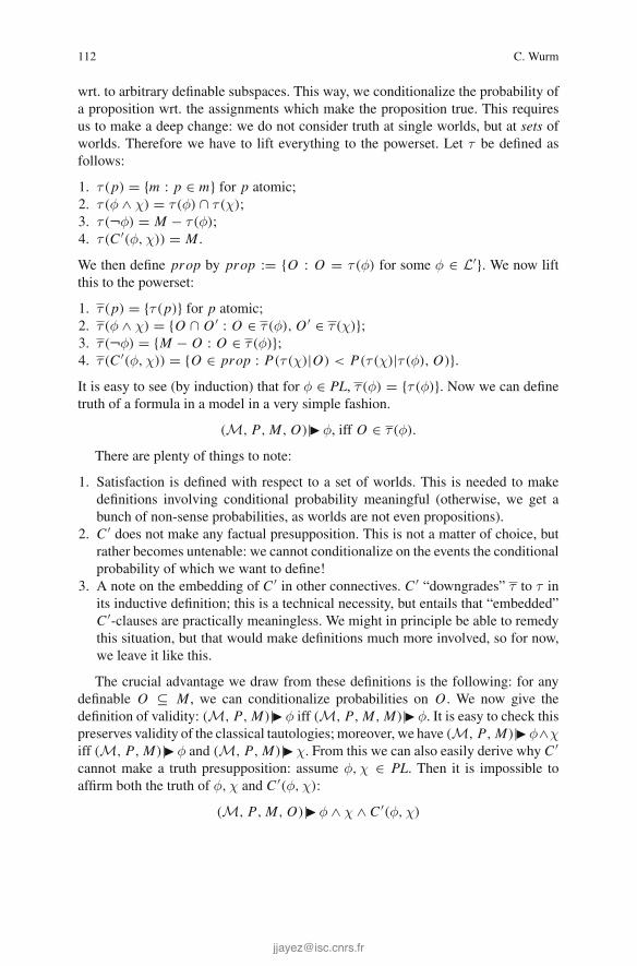
112 C. Wurm
wrt. to arbitrary definable subspaces. This way, we conditionalize the probability ofa proposition wrt. the assignments which make the proposition true. This requiresus to make a deep change: we do not consider truth at single worlds, but at sets ofworlds. Therefore we have to lift everything to the powerset. Let τ be defined asfollows:
1. τ (p) = {m : p ∈ m} for p atomic;2. τ (φ ∧ χ) = τ (φ) ∩ τ (χ);3. τ (¬φ) = M − τ (φ);4. τ (C ′(φ,χ)) = M .
We then define prop by prop := {O : O = τ (φ) for some φ ∈ L′}. We now liftthis to the powerset:
1. τ (p) = {τ (p)} for p atomic;2. τ (φ ∧ χ) = {O ∩ O ′ : O ∈ τ (φ), O ′ ∈ τ (χ)};3. τ (¬φ) = {M − O : O ∈ τ (φ)};4. τ (C ′(φ,χ)) = {O ∈ prop : P(τ (χ)|O) < P(τ (χ)|τ (φ), O)}.It is easy to see (by induction) that for φ ∈ PL, τ (φ) = {τ (φ)}. Now we can definetruth of a formula in a model in a very simple fashion.
(M, P, M, O)|� φ, iff O ∈ τ (φ).
There are plenty of things to note:
1. Satisfaction is defined with respect to a set of worlds. This is needed to makedefinitions involving conditional probability meaningful (otherwise, we get abunch of non-sense probabilities, as worlds are not even propositions).
2. C ′ does not make any factual presupposition. This is not a matter of choice, butrather becomes untenable: we cannot conditionalize on the events the conditionalprobability of which we want to define!
3. A note on the embedding of C ′ in other connectives. C ′ “downgrades” τ to τ inits inductive definition; this is a technical necessity, but entails that “embedded”C ′-clauses are practically meaningless. We might in principle be able to remedythis situation, but that would make definitions much more involved, so for now,we leave it like this.
The crucial advantage we draw from these definitions is the following: for anydefinable O ⊆ M , we can conditionalize probabilities on O . We now give thedefinition of validity: (M, P, M)|� φ iff (M, P, M, M)|� φ. It is easy to check thispreserves validity of the classical tautologies; moreover, we have (M, P, M)|� φ∧χiff (M, P, M)|� φ and (M, P, M)|� χ. From this we can also easily derive why C ′cannot make a truth presupposition: assume φ,χ ∈ PL. Then it is impossible toaffirm both the truth of φ,χ and C ′(φ,χ):
(M, P, M, O)|� φ ∧ χ ∧ C ′(φ,χ)
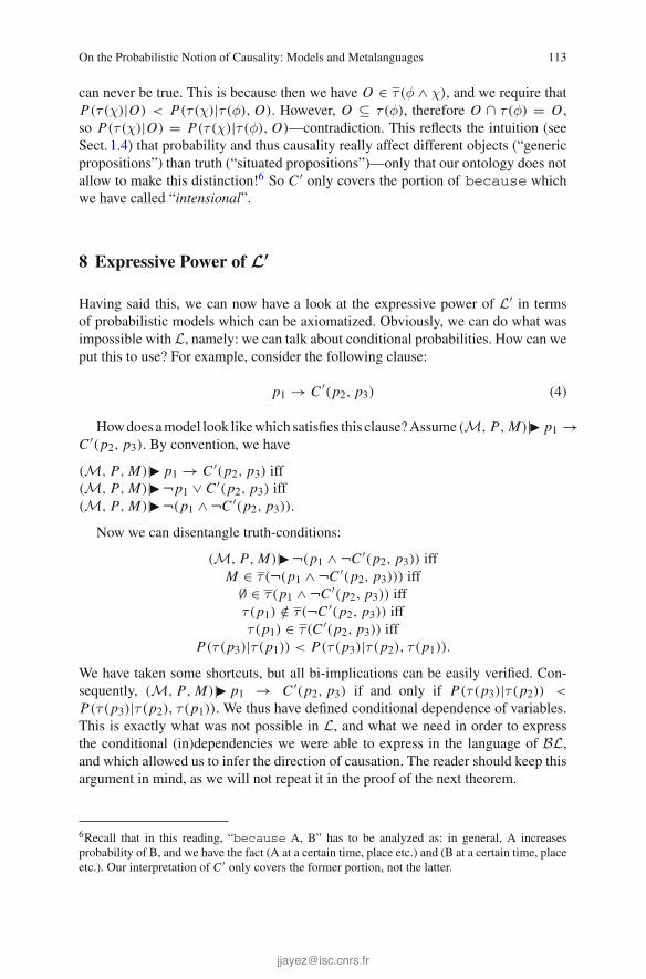
On the Probabilistic Notion of Causality: Models and Metalanguages 113
can never be true. This is because then we have O ∈ τ (φ ∧ χ), and we require thatP(τ (χ)|O) < P(τ (χ)|τ (φ), O). However, O ⊆ τ (φ), therefore O ∩ τ (φ) = O ,so P(τ (χ)|O) = P(τ (χ)|τ (φ), O)—contradiction. This reflects the intuition (seeSect. 1.4) that probability and thus causality really affect different objects (“genericpropositions”) than truth (“situated propositions”)—only that our ontology does notallow to make this distinction!6 So C ′ only covers the portion of because whichwe have called “intensional”.
8 Expressive Power of L′
Having said this, we can now have a look at the expressive power of L′ in termsof probabilistic models which can be axiomatized. Obviously, we can do what wasimpossible with L, namely: we can talk about conditional probabilities. How can weput this to use? For example, consider the following clause:
p1 → C ′(p2, p3) (4)
Howdoes amodel look likewhich satisfies this clause?Assume (M, P, M)|� p1 →C ′(p2, p3). By convention, we have
(M, P, M)|� p1 → C ′(p2, p3) iff(M, P, M)|� ¬p1 ∨ C ′(p2, p3) iff(M, P, M)|� ¬(p1 ∧ ¬C ′(p2, p3)).
Now we can disentangle truth-conditions:
(M, P, M)|� ¬(p1 ∧ ¬C ′(p2, p3)) iffM ∈ τ (¬(p1 ∧ ¬C ′(p2, p3))) iff
∅ ∈ τ (p1 ∧ ¬C ′(p2, p3)) iffτ (p1) /∈ τ (¬C ′(p2, p3)) iffτ (p1) ∈ τ (C ′(p2, p3)) iff
P(τ (p3)|τ (p1)) < P(τ (p3)|τ (p2), τ (p1)).
We have taken some shortcuts, but all bi-implications can be easily verified. Con-sequently, (M, P, M)|� p1 → C ′(p2, p3) if and only if P(τ (p3)|τ (p2)) <
P(τ (p3)|τ (p2), τ (p1)). We thus have defined conditional dependence of variables.This is exactly what was not possible in L, and what we need in order to expressthe conditional (in)dependencies we were able to express in the language of BL,and which allowed us to infer the direction of causation. The reader should keep thisargument in mind, as we will not repeat it in the proof of the next theorem.
6Recall that in this reading, “because A, B” has to be analyzed as: in general, A increasesprobability of B, and we have the fact (A at a certain time, place etc.) and (B at a certain time, placeetc.). Our interpretation of C ′ only covers the former portion, not the latter.

114 C. Wurm
Our main theorem will now be the following: for any finite collection of BL-formulas, there is an L′ formula φ, such that for any probabilistic model, it is amodel of the one if and only if it is a model of the other.
Theorem 10 For each finite B ⊆ BL, there is a φ ∈ L′, such that for every proba-bilistic model (M, P, M), (M, P, M)|� φ if and only if (M, P, M) � B.
Proof LetB be a finite collection ofBL-clauses. There are two types of these clauses,the ones constructed from ‖ and those with ∦. As in L′, we have negation, there isno problem in getting from one to the other; and as we have conjunction, there isno problem in getting from single clauses to finite collections. So the problem boilsdown to only two kinds of BL-clauses we have to show we can translate into L′:firstly for statements of the type:
(φi ∦ φ j |φl).
By definition of BL, we know that φi ,φ j ,φl ∈ PL, and thus in L′. We can quiteeasily translate this into an L′-formula as follows:
(φi ∦ φ j |φl)+ := (φl) → (C ′(φi ,φ j ) ∨ C ′(φi ,¬φ j ))
We can verify that this has the desired meaning; we shorten the proof because wealready showed large part of it by the above considerations. Note however that it iscrucial thatφi ,φ j ,φl ∈ PL, such that we have τ (φi ) = {τ (φi )} etc. Now assume that(M, P, M, O)|� φl . Then we must have either P(τ (φ j )|O) < P(τ (φ j )|τ (φi ), O)
or P(τ (¬φ j )|O) < P(τ (¬φ j )|τ (φi , O). Now, by definition of ¬ and probabilityaxioms, it is clear that if P(τ (φ j )|O) = P(τ (φ j )|τ (φi ), O), then both are false,so the translation works as required. As negation in L′ is fully classical, this is alsosufficient for (φi‖φ j |φl), which is equivalent to ¬(φi ∦ φ j |φl).
Regarding BL-formulas of the form (φi‖φ j ), we simply translate them by
(φi‖φ j )+ := C ′(φi ,φ j ) ∨ C ′(φi ,¬φ j )
Finally, to finish the proof, we simply observe that B is a finite set of clauses,and (M, P, M) � B if (M, P, M) � φ for all φ ∈ B. Let [−]+ be the trans-lation from BL to L′. Then, by definition of ∧, (M, P, M) � B if and only if(M, P, M)|� ∧
φ∈B φ+, which is a finite conjunction and therefore an L′-sentence.�
Note that the inverse of Theorem 10 is obviously false:L′ ismuchmore expressivethanBL for several reasons: we cannot specify a setB ⊆ BL such that (M, P, M) �B if andonly if P(Ei |E j )> P(Ei );we canonly talk about independence.Theorem10is extremely important for the following reason: in the same fashion as BL givesus proper information about the directionality of causation—under suitable sideassumptions—, the same holds for L′: given a sufficiently rich source of L′ clauses,we can infer in which direction causality goes.
Note however that the question of inferences is a topic of its own right, and canbe conceived of in several fashions: in the first conception, we just have an L′-clauseφ; it might be that φ, as some knowledge on the world, encodes the directionality of

On the Probabilistic Notion of Causality: Models and Metalanguages 115
causation of two events E1, E2. That does of course not mean that we can imme-diately see or verify this: to “decode” directionality of causation from φ might bea difficult problem, on which we have said nothing so far, and we think this willrequire an investigation on its own. The more obvious conception is the following:assumewe have a givenmodel (M, P, M), where P can be effectively computed (orapproximated). As we have seen above, given two events E1, E1 ⊆ M , there are twoBL-clauses φ,ψ, such that if (M, P, M) � {φ,ψ}, then there is a directional causallink from E1 to E2. By Theorem 10, this means: we can also just check whether(M, P, M)|� φ+ ∧ ψ+, and thereby establish a causal link. The |� relation, as longas P is computable, can easily be shown to be decidable.
So for L′ as for all our languages we have to keep in mind: when we say someformula (or set of formulas) encodes the directionality of causation, we mean: wecan infer this information from the formula, but it cannot be expressed in the lan-guage itself (not even in the broadest sense, because this would require some sort ofquantification over propositions)! This situation does not seem undesirable, when wecompare to the situation to natural language: there is no syntactic difference betweenproper and epistemic usage of because (at least not across the board, though thereare preferences in certain constellations). Nonetheless, “semantically”, we have clearintuitions about the two.
9 Conclusion
We have presented several “languages of causality”, namely BL, L and L′. State-ments in BL can be read as denoting the (un)conditional (in)dependence of events;this language is well-known as a meta-language for Bayesian networks, and can beused to uniquely encode the directionality of a link in a minimal Bayesian networkmodelling the distribution under discussion. We have introduced and investigatedthe languages L,L′ and their semantics, because they are closer to our intuitionabout causation being a binary relation, which can in turn be embedded arbitrarilyin other connectives. The main question was: how expressive in terms of axiom-atization of probability spaces are these logical languages? BL served for us as atouch-stone: if any of the languages L,L′ can encode BL-statements, it can encodethe directionality of causation. We have shown that L is not sufficiently expressive,in particular, it cannot even express the notion of a conditional probability. On theother hand,L′ turns out to be powerful enough to encode arbitrary (finite sets of) BLstatements.
Thoughwehave settled these questions, there aremanyquestions left open, amongwhich most prominently: given L,L′ and their semantics, is there a purely syntactic,proof-theoretic way to determine consequence and validity? And in particular, a wayto determinewhether a given set of formulas encodes a particular kindof dependency?That seems an interesting, difficult problem. The next question is: let |=, |� denoteconsequence relations between (sets of) formulas in the usual fashion, that is:Γ |= φif for all γ ∈ Γ , (M, P, M) |= γ, then (M, P, M) |= φ. What properties do

116 C. Wurm
these relation have? Do they behave like normal, logical consequence relations,being monotonous, finitary, closed under substitution etc.? This also seems far fromobvious. These seem to us the most natural questions to address next.
References
Dehgani, M., Iliev, R., & Kaufmann, S. (2012). Causal explanation and fact mutability in counter-factual reasoning. Mind & Language, 27(1), 55–85.
Ebbinghaus, H.-D., & Flum, J. (1995). Finite Model Theory. Perspectives in Mathematical Logic.Springer.
Geiger, D., & Pearl, J. (1990). Logical and algorithmic properties of independence and their appli-cation to Bayesian networks. Annals of Mathematics and Artificial Intelligence, 2, 165–178.
Kaufmann, S. (2009). Conditionals right and left: Probabilities for the whole family. Journal ofPhilosophical Logic. 38(1), 1–53.
Koller, D., & Friedman, N. (2009). Probabilistic graphical models: Principles and techniques.Adaptive computation and machine learning. MIT Press, Cambridge.
Pearl, J., (2009). Causality. Models, Reasoning, and Inference. Cambridge University Press,Cambridge.
Schurz, G., & Leitgeb, H. (2008). Finitistic and frequentistic approximation of probability measureswith or without σ-additivity. Studia Logica, 89(2), 257–283.
Verma, T., & Pearl, J. (1990). Equivalence and synthesis of causal models. In P. P. Bonissone, M.Henrion, L. N. Kanal, & J. F. Lemmer, (Eds.), UAI, (pp. 255–270). Elsevier.
Wachter, B., Zhang, L., & Hermanns, H. (2007). Probabilistic model checking modulo theories. InQEST, (pp. 129–140). IEEE Computer Society.
Woodward, J. (2003). Making things happen: A theory of causal explanation. Oxford: OxfordUniversity Press.
Woodward, J. (2006). Sensitive and insensitive causation. The Philosophical Review, 115, 1–50.
Shannon Versus Chomsky: Brain Potentialsand the Syntax-Semantics Distinction
Mathias Winther Madsen
Abstract The N400 and the P600 are two patterns of electrical brain potentialswhich can sometimes be found when people read or hear unexpected words. Theyhave been widely claimed to be the neurological correlates of semantic and syntac-tic anomalies, respectively, but evidence accumulated over the last decade has raisedsome serious doubts about that interpretation. In this paper, I first review some of thisevidence and then present an alternative way to think about the issue. My suggestionis built on Shannon’s concept of noisy-channel decoding by tables of typical sets, andit is thus fundamentally statistical in nature. I show that a proper application of Shan-non’s concepts to the reading process provides an interesting reinterpretation of ournotion of “syntax,” thus questioning some fundamental assumptions of linguistics.
Keywords N400 · P600 · Electroencephalography · Psycholinguistics · Informa-tion theory · Probabilistic inference · Noisy-channel models · Syntax-semanticsinterface · Autonomy of syntax
One of the key ideas that helped establish linguistics as a respectable science in the1950s was the idea that the processing of syntax is carried out by an autonomous men-tal module that works independently of the processing of meaning. Noam Chomskyfamously pushed this point by presenting sentence pairs that seemed to dissociate vio-lations of syntactic expectations from violations of semantic expectations (Chomsky1957, pp. 15–16):
• The child seems sleeping (syntactic anomaly)• Today I saw a fragile whale (semantic anomaly)
M.W. Madsen (B)Institute for Logic, Language and Computation,University of Amsterdam, Amsterdam, The Netherlandse-mail: [email protected]
© Springer International Publishing Switzerland 2015H. Zeevat and H.-C. Schmitz (eds.), Bayesian Natural Language Semanticsand Pragmatics, Language, Cognition, and Mind 2,DOI 10.1007/978-3-319-17064-0_6
117

118 M.W. Madsen
Based on such examples, he concluded that violations of syntactic rules had nothingto do with the meaning of the words in the sentence, and thus
… we are forced to conclude that grammar is autonomous and and independent of meaning,and that probabilistic models give no particular insight into some of the basic problems ofsyntactic structure (Chomsky 1957, p. 17).
While the introspective case from example sentences was Chomsky’s strongest argu-ment at the time, he did imagine hypothetical psychological experiments that couldbe used to corroborate his claim, such as memory or reading tests that could perhapsdistinguish “ungrammatical” sentences from mere nonsense (Chomsky 1957, p. 16).
This paper is about one attempt to realize such a research program. As I shallexplain shortly, the brain sciences found some new results in the 1990s which seemedto finally put Chomsky’s claims on a solid scientific basis. For a period of about tenyears, the consensus was accordingly that the anatomical and psychological realityof Chomsky’s little syntactic engine was a scientific fact. Syntax had acquired theauthority of being “brain stuff.”
In one sense, this paper is an elaborate criticism of this idea. I will review a wealthof empirical evidence from the last decade which seriously complicates the pictureof the brain phenomena that were originally used to vindicate the Chomskyan viewof language. Even a casual look at this literature exposes an abundance of unrulylittle details that fit very badly into the old pigeonholes.
But this is also a constructive paper: I propose a precise computational model thatmay explain much of the psychological evidence. This model is based on a seeminglyinsignificant idea about statistical error used by Claude Shannon in the 1948 paperwhich founded the field of information theory (Shannon 1948).
This idea has some deep connections to the foundations of statistical inference andthus to the notion of rational decision-making in the most general sense. Presentingmy model will thus require a detour around some basic concepts from informationtheory and statistics. Once I have introduced those concepts, I will focus on a morespecific example of a decoding problem similar to the experimental situations usedin the psychological literature. I will then discuss how that toy problem might bescaled up to give accurate, quantitative predictions.
1 The N400 and the P600
In this section, I will introduce the brain phenomena that are pivot of the entire paper.These phenomena are a couple of distinctive changes in the electrical brain potentialthat can be measured off the scalp of a person’s head during reading, listening, orother activities. Only in the next section will I discuss in more detail how we shouldinterpret these modulations of the brain potential.

Shannon Versus Chomsky: Brain Potentials … 119
1.1 The N400
Suppose I present you with a sentence by flashing each word on a computer screenat regular intervals:
• I … spread … the … warm … toast … with …
While you are reading the sentence, I am recording the electrical activity at differentplaces on the top of your head. Since all nerves in your body change the electricalfield around them when they are excited, this recording provides an estimate of howactive the nerves inside your head are. By using the electrical activity in the head asa measure of cognitive effort, this experimental paradigm can thus reveal whethera sentence requires more effort than usual to read, and where in the sentence theproblems begin.
This means that rather specific differences between sentences can be compared. Icould, for instance, change a single word in a sentence and then compare the patternof electrical activity that arises when you read the original sentence with the patternassociated with the manipulated one:
• I spread the warm toast with butter (original)• I spread the warm toast with socks (manipulation)
This manipulation was the idea behind an experiment which was first carried outby Martha Kutas and Steven A. Hillyard in 1980, and which has since then beenreplicated many times. Their experiment involved a set of sentence pairs like the onesabove: One completely unproblematic sentence and one that ended in a “semanticallyinappropriate (but syntactically correct)” word (Kutas and Hillyard 1980, p. 203).
By averaging over several subjects’ responses to the two versions of the sentences,Kutas and Hillyard found that the oddness of the manipulated sentences tended toevoke a characteristic electrical response characterized by an excess of negativeelectrical potential relative to the control condition (Fig. 1).
Fig. 1 A graph from Kutas and Hillyard (1980, p. 204) showing the averaged response to theinappropriate word (e.g., socks) minus the averaged response to the appropriate (e.g., butter). Bothwaveforms were recorded by an electrode at the back of the head (the medial parietal position). Asis conventional in electrical engineering, negative charge is plotted as up
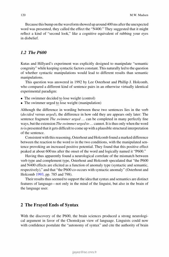
120 M.W. Madsen
Because this bump on the waveform showed up around 400 ms after the unexpectedword was presented, they called the effect the “N400.” They suggested that it mightreflect a kind of “second look,” like a cognitive equivalent of rubbing your eyesin disbelief.
1.2 The P600
Kutas and Hillyard’s experiment was explicitly designed to manipulate “semanticcongruity” while keeping syntactic factors constant. This naturally led to the questionof whether syntactic manipulations would lead to different results than semanticmanipulations.
This question was answered in 1992 by Lee Osterhout and Phillip J. Holcomb,who compared a different kind of sentence pairs in an otherwise virtually identicalexperimental paradigm:
• The swimmer decided to lose weight (control)• The swimmer urged to lose weight (manipulation)
Although the difference in wording between these two sentences lies in the verb(decided versus urged), the difference in how odd they are appears only later: Thesentence fragment The swimmer urged … can be completed in many perfectly fineways, but the extension The swimmer urged to … cannot. It is thus only when the wordto is presented that it gets difficult to come up with a plausible structural interpretationof the sentence.
Consistent with this reasoning, Osterhout and Holcomb found a marked differencebetween the reaction to the word to in the two conditions, with the manipulated sen-tence provoking an increased positive potential. They found that this positive effectpeaked at about 600 ms after the onset of the word and logically named it “P600.”
Having thus apparently found a neurological correlate of the mismatch betweenverb type and complement type, Osterhout and Holcomb speculated that “the P600and N400 effects are elicited as a function of anomaly type (syntactic and semantic,respectively),” and that “the P600 co-occurs with syntactic anomaly” (Osterhout andHolcomb 1993, pp. 785 and 798).
Their results thus seemed to support the idea that syntax and semantics are distinctfeatures of language—not only in the mind of the linguist, but also in the brain ofthe language user.
2 The Frayed Ends of Syntax
With the discovery of the P600, the brain sciences produced a strong neurologi-cal argument in favor of the Chomskyan view of language. Linguists could nowwith confidence postulate the “autonomy of syntax” and cite the authority of brain

Shannon Versus Chomsky: Brain Potentials … 121
science as support (see e.g. Fernández and Cairns 2010, Chap. 3). The issues raised byChomsky from a purely introspective perspective finally seemed to be settled byempirical investigations.
The issue is, however, not quite as simple as this. Within the last decade, a numberof experiments have documented P600 responses to sentences that are not syntacti-cally anomalous in any usual sense of the word “syntax.” I will spend the remainder ofthis section illustrating these complications in some detail, drawing quite heavily onan excellent review paper by Gina Kuperberg (2007). For a more exhaustive reviewof the wide variety of contexts in which the N400 is found, including non-linguisticcontexts, see Kutas and Federmeier (2011).
2.1 Word Shuffling and P600 Effects
One of the first indications that the P600 could not unproblematically be equatedwith broken syntax came from a Dutch study which manipulated the test sentencesby changing a passive construction into an active, causing the logical subject and thelogical object swap roles (Hoeks et al. 2004).
In Dutch, the main content verb is often placed at the very end of the sentence,as in The boy has the ball kicked. If you read such a verb-final sentence in a word-for-word presentation, a whole string of nouns and auxiliary verbs can thus be pre-sented to you before you finally reach the main content verb (here kicked). Thismeans that one can construct a Dutch sentence such that it creates a very strongexpectation as to what the final verb will be, and those expectations can then beviolated or respected.
This grammatical fact was exploited in the materials used by Hoeks et al. Theyconstructed three different manipulated sentences from a control by substitutingeither the main content verb, an auxiliary verb, or both:
• De eed werd door de jonge artsen afgelegd.(“The oath was taken by the young doctors.”)
• De eed werd door de jonge artsen behouden.(“The oath was kept/retained by the young doctors.”)
• De eed heeft de jonge artsen afgelegd.(“The oath has taken the young doctors.”)
• De eed heeft de jonge artsen behouden.(“The oath has kept/retained the young doctors.”)
The manipulations of the main verb (e.g., substituting retain an oath for take an oath)tended to produce mere nonsense, and as expected, this manipulation produced anN400 effect. However, the manipulation of the auxiliary verb—which caused thesubject and object to change roles—unexpectedly triggered an excess of late positivepotential beginning around 600 ms after the final verb (cf. Fig. 2).
Although both of these manipulations resulted in a grammatical sentence, onlyone of them would produce an N400, and the other would instead produce a very

122 M.W. Madsen
“The deck of cards has shuffled the gamblers.”
“The deck of cards has hit the gamblers.”
“The deck of cards was hit by the gamblers.”
Fig. 2 Averaged single-electrode recordings from Hoeks et al. (2004, p. 68), with positive chargeplotted as up. The three waves show the differences in voltage between the three manipulatedconditions and the control condition (“The deck of cards was shuffled by the gamblers”). All threewaveforms exhibited a significant P600 effect at this electrode
pronounced P600. This ran directly counter to the notion that the P600 exclusivelytracks syntactic problems.
Similar effects were reported for English. In one 2003 experiment, Kuperberget al. compared two different kinds of unexpected verbs and again found that onlysome of them provoked an N400 response:
• For breakfast, the boys would only eat … (control)• For breakfast, the boys would only bury … (N400)• For breakfast, the eggs would only eat … (P600)
Kuperberg et al. suggested that this difference might be explained in terms of thethematic roles prescribed by a verb like eat, assuming that “the P600 is sensitive toviolations in this thematic structure” (Kuperberg et al. 2003, p. 127).
This line of thought was also supported by another study which compared merenonsense to bizarre subject-verb combinations (Kim and Osterhout 2005). This study,too, found marked differences in the kinds of response elicited by the two manipu-lations relative to a control condition of ordinary English:
• The library books had been borrowed by the graduate student. (control)• The tragic mistake was borrowing in a hurry. (N400)• The library books had been borrowing the graduate student. (P600)
Like Kuperberg et al., Kim and Osterhout suspected that the difference between thetwo target sentences had something to do with how nouns plug into verbs. Theyformulated this intuition in terms of a “semantic attraction to particular predicate–argument combinations” (Kim and Osterhout 2005, p. 215).
2.2 Animacy and Related Criteria
Looking at these examples, one might come to expect that the crucial issue herehad something to do with animacy: boys are animate and therefore appropriate sub-jects for the verb eat, but eggs are not. However, as several authors have argued,
Shannon Versus Chomsky: Brain Potentials … 123
this distinction does not quite capture the differences in the empirical material(Kuperberg et al. 2003; Kuperberg 2007).
For instance, library books and tragic mistakes are both inanimate noun phrases,and both are inappropriate as subjects for the verb borrow. Still, the construction thelibrary books borrowed elicits a P600, while the tragic mistakes borrowed elicits anN400, as mentioned above. Since these constructions are equivalent in terms of ani-macy violations, this dimension alone is thus an unreliable predictor of P600 effects.
It should also be kept in mind that many earlier experiments had used subject-verbcombinations that were clearly illegitimate in terms of animacy and other selectioncriteria, but still produced N400 effects instead of P600 effects. One German study,for instance, used the following target sentences:
• Der Honig wurde ermordet.(“The honey was murdered.”)
• Der Ball hat geträumt.(“The ball has dreamt.”)
Both of these sentence types provoked a marked N400 response, but no P600(Rösler et al. 1993). It would thus appear that inanimate objects can be used withverbs that require animate subjects without provoking a P600 (although this willprobably produce an N400).
As for the opposite implication—P600 effects predicting animacy violations—other research groups have also documented P600 responses to sentences in whichanimate subjects do clearly animate things. One study by Kolk et al. (2003), forinstance, found this in Dutch sentences like
• De vos die op de stropers joeg …(“The fox that was hunting the poachers …”)
• De kat die voor de muizen vluchtte …(“The cat that was fleeing the mice …”)
Of course, the roles are in some sense swapped in this sentence—but since both foxesand poachers are animate, the strangeness of these sentences cannot be described interms of animacy alone.
In another experiment applying essentially the same materials, van Herten et al.(2005, p. 249) to their own surprise, also found P600 effects for sentences such as
• De bomen die in het park speelden …(“The trees that played in the park …”)
In a later paper, they hypothesized that this P600 effect was caused by the strongsemantic relation between the words (one can play in a park full of trees) incombination with the oddness of the sentence as a whole (the trees played). Oneway of describing this pattern could be that it involves nouns and verbs thattend to occur in the same contexts, but rarely in subject-predicate combinations(van Herten et al. 2006).
124 M.W. Madsen
This theory would explain differences such as the following:
• Jan zag dat de olifanten de bomen snoeiden en …(“John saw that the elephants pruned the trees and …”—P600)
• Jan zag dat de olifanten de bomen verwenden en …(“John saw that the elephants spoiled the trees and …”—N400)
Trees, elephants, and pruning can easily occur in the same text or even the samesentence, but it is rarely the elephants that are doing the pruning. On the other hand,spoiling (as in spoiling a child) is semantically unrelated to elephants and trees, andthe word tends to occur in very different contexts.
Whether this exact formulation of the theory is correct or not, there are thus quitestrong reasons to doubt that the conditions producing the P600 is a matter of pluggingan inanimate noun into a verb frame that requires an animate argument, or vice versa.A wide variety of word relationships seem to be responsible for turning “semantic”anomalies into potentially “syntactic” ones.
2.3 Grammatically Ungrammatical
Given all of this data, it seems that there is no clear and straightforward relationshipbetween the P600 and the arguments that can be plugged into a verb. The issue doesnot seem to be syntactic well-formedness, nor does it seem to be about animacy orthematic structure. It might still be the case, however, that some other grammaticalparameter—say, aspect, mood, gender, number—is the key. But even this vaguesuggestion has some empirical evidence against it.
One such piece of evidence comes from a study that recycled some sentenceswhich had already previously been shown to produce strong and reliable N400 effects.In this experiment, an elaborate context was prepended to the test sentences, andthe brain potentials were recorded in the same manner as in the previous study(Nieuwland and Van Berkum 2005).
One of stories used in this experiment read as follows, in translation from theoriginal Dutch:
• A tourist wanted to bring his huge suitcase onto the airplane. However, because thesuitcase was so heavy, the woman behind the check-in counter decided to chargethe tourist extra. In response, the tourist opened his suitcase and threw some stuffout. So now, the suitcase of the resourceful tourist weighed less than the maximumtwenty kilos. Next, the women told the suitcase that she thought he looked reallytrendy. …
Surprisingly, this long build-up to the crucial unexpected word completely canceledthe N400 effect found in the original study and instead produced a strong P600 effect.Thus, the manipulation of the context which turned the suitcase into a prop in thenarrative dramatically changed the way the subjects read the nonsense sentence thewoman told the suitcase.
Shannon Versus Chomsky: Brain Potentials … 125
But perhaps the deepest problem with the idea that the P600 can be describedin grammatical terms is that it can be provoked by sentences without any syntacticanomalies at all. This was already shown in a study from 1999 (Weckerly and Kutas1999) which compared sentences of the following form:
• The novelist that the movie inspired praised the director for …• The editor that the poetry depressed recognized the publisher of the …
Strictly speaking, there is nothing semantically or syntactically anomalous aboutmovies that inspire novelists, or about poetry that depresses editors. Still, these con-structions tended to produce a P600 response.
Weckerly and Kutas used these findings in order to make a point about “theuse of animacy information in the processing of a very difficult syntactic structure”(Weckerly and Kutas 1999, p. 569). Their findings may also have more specificcauses, though, such as the strong, conventional expectations carried by word clusterslike novelist, movie, and inspire. However, since their experimental materials were notreprinted in the paper, it is hard to assess how strong the case for such an explanationmight be.
However, regardless of these points of interpretation, it seems clear that there aresome serious problems with seeing the P600 as the exhaust pipe of a syntacticalprocessor in the brain: There are several kinds of semantic oddness that are quitestrongly related to the P600; it can be quite heavily modulated by discursive context;and it can even be elicited by grammatical sentences. The standard tools from thetoolbox of theoretical linguistics thus seem to have some problems getting to gripswith this phenomenon.
I take this as a sign that we need to back up a bit and take a fresh look at ourassumptions. In the next section, I will consequently suggest that in order to under-stand the brain processes behind the N400 and the P600, we need to go all the wayback to Chomsky, and then go a little further back.
3 The Statistics of Decoding: Errors of Type I and II
In the preceding section, I have presented a number of empirical phenomena thatseriously challenges the traditional identification of the N400 and the P600 withsemantic and syntactic anomaly, respectively. As the examples have shown, the P600in particular crops up in a number of different circumstances that cannot be equatedwith broken syntax without bending our notion of syntax completely out of shape.This raises two questions.
1. We might wonder whether there is any system at all to where the P600 is present.Indeed, after looking at the wide variety of examples in the previous section, onemight get the impression that brain potentials just aren’t the kind of phenomenathat can be adequately predicted. It is an open question whether we can evendescribe the phenomenon in intuitive terms, and whether we can look at a sentenceand guess what kind of brain response it will evoke.

126 M.W. Madsen
2. Assuming that there is some kind of system, the question is what formalismwould be most suited to articulate it. It is tempting to pull down the grammaticalvocabulary from the shelf, since we are after all talking about language; but it isnot a given that a theory of the N400 and the P600 should come in such a form,or that it should involve any concepts from Chomskyan linguistics.
In this section, I will suggest that there is indeed a way of understanding the twobrain components of the reading-related brain potentials, but that they have little todo with language as such. Instead, I will draw on some classical statistical insightsfrom information theory (Shannon 1948) and approach the activity of reading as akind of decoding problem. The two brain responses will then show up as correlatesof two particular kinds of decoding error.
This suggestion is consistent with an intuition shared by many researchers in thefield, namely, that the P600 is some kind of “error-correction signal” (Gibson et al.2013, p. 8055) or the electrical counterpart of a “monitoring process triggered by aconflict between two or more incompatible representations” (van Herten et al. 2006,p. 1195; see also Frenzel et al. 2011).
Similarly, Kolk et al. (2003) note that both the N400 and the P600 are triggeredby unexpected events, and they add:
The problem with such events is that they can have two sources. They can be real, in thesense that an unexpected event has indeed occurred. On the other hand, they can also stemfrom a processing error (Kolk et al. 2003, p. 31).
To paraphrase this in information-theoretic terms, strange things can either happenin the source or in the channel. I agree completely with this intuition, and the purposeof this section is to spell it out in some more mathematical detail. The model thatI will present is very similar to the one discussed by Gibson et al. (2013, p. 8055),both in its general philosophy and in the mathematical detail. I will, however, be a bitmore explicit in my claims about the N400 and the P600 (which they only mention inpassing), in particular when it comes to identifying their exact computational-levelcounterparts.
I will claim that the two electrical responses correspond to two different kindsof decoding error: The P600 is present when there are too many candidate causesthat match an observed effect, and the N400 is present when there are none. Thishypothesis draws on an idea that Shannon used in the proof of his discrete channelcoding theorem (Shannon 1948, Theorem 11) and which was later made more explicitby others (Cover 1975; Cover and Thomas 1991, Chap. 7.7). Shannon operationalizedthe notion of a “match” between a cause and an effect in terms of a concept called the“typical set.” This set contains, as I shall explain in more detail below, the events thatare about as probable as one would expect an event to be (Shannon 1948, Theorem 3).
Before I can formulate my hypothesis about the difference between the N400 andthe P600, I will first have to discuss this concept and a few other basic notions frominformation theory. I will then illustrate the idea behind my theory by showing howit works in a computationally simple case, and then hint at what it would look likein a more realistic model.

Shannon Versus Chomsky: Brain Potentials … 127
3.1 Typical Sets and Most Probable Sets
One of building blocks of information theory is the concept of a “typical set”(Shannon 1948, Theorem 3). The typical set associated with an experiment is theset of outcomes whose logarithmic probabilities are close to the expected logarith-mic probability.
To put this differently, suppose we identify the experiment in question with arandom variable X and that we let p(x) be the probability of the event X = x .As suggested by Samson (1951), we can then think of the number − log p(x) asa quantification of how “surprising” the observation X = x is. This “surprisal” isa number between 0 and ∞, with less probable events having a higher surprisalvalues (cf. Fig. 3).
A random variable X which can take different values with different probabilitiesthus always corresponds implicitly to a “surprisal” variable − log p(X) which rangesover the set of surprisal values. The expected value of this surprisal variable isH = H(X), the entropy of X .
Using these concepts, we can then reformulate the definition of the typical set: Itis the set of events X = x whose surprisal value is close to the average surprisal. Fora fixed ε > 0, the ε-typical set of a random variable X thus contains the x for which
∣∣∣∣ log1
p(x)− H
∣∣∣∣ ≤ ε.
The ε-typical set associated with an experiment does not necessarily include themost probable outcome of the experiment. However, as mentioned by Shannon (1948,Theorem 3) and explained in more detail by Cover and Thomas (1991, Chap. 3.3),the set of outcomes that are less surprising than H usually differs very little from thetypical set, since any two high-probability sets must have a high-probability overlap.Specifically, if the values of the random variable X are long sequences from an
Fig. 3 Left The probability of getting a sum of Σ = 5, 6, 7, . . . , 30 in 5 dice throws, with the typicalprobability 2−H shown as a dotted line. Right The same, plotted on an inverse logarithmic scale

128 M.W. Madsen
Fig. 4 Sequences of length N = 25 from an ergodic source. The entropy rate of the source isH = 0.80 bits per symbol
ergodic random process (such as strings of letters or words; cf. Fig. 4), then includingthe most probable outcomes will only change the size and total probability of theset slightly. In many important respects, it thus makes little difference whether wedefine the typical set by the bound − log p(x) ≤ H + ε or the symmetric conditionH − ε ≤ − log p(x) ≤ H + ε.
3.2 Decoding by Jointly Typical Sets
The conditions discussed above define the typical set for a single random variable. Inthe context of information transmission, however, we are rarely interested in a single,isolated variable, but much more often in the relationship between two variables Xand Y that model a cause and an effect, or a transmitted message and a receivedsignal.
In order to study such relationships, it is useful to consider the typical sets asso-ciated with the joint stochastic variable X × Y . This set consists of pairs (x, y) thatare typical with respect to the joint probability distribution on X × Y , and it is calledthe jointly typical set.
In an information transmission context, a jointly typical pair (x, y) consists ofa high-probability message x and a noisy signal y which has a high probabilitygiven the message. The set of all such pairs collectively describe the properties of thecommunication channel modeled by X ×Y . A model of written English, for instance,might include (forty, fourty) as a typical pair, since forty is a common word, and fourtya common misspelling of it. Other channels will have other characteristic types ofconfusability (cf. Fig. 5).
This way of looking at the issue suggests that a table of the typical pairs could beused for decoding: When you receive a message y, you just skim through the table,find a pair of the form (x, y), and then return x as your decoded message. Althoughthis hypothetical algorithm is usually not feasible in its naive form, it captures manyof the conceptual ideas about channel coding, and its complexity problems are largelyirrelevant to the point I want to make here.

Shannon Versus Chomsky: Brain Potentials … 129
Fig. 5 One possible structure of a jointly typical set for increasing tolerance thresholds and thusdecreasing lower bounds on the joint probability p(x, y)
3.3 Two Types of Decoding Error
As is apparent from the description of the hypothetical brute-force algorithm fordecoding by jointly typical sets, two distinct problems can arise for a decoder:
1. There is no x for which (x, y) is typical2. There is more than one x for which (x, y) is typical
As an illustration of these two types of error, suppose that the message is one of twopoints in the plane, A or B, and that the received signal is equal to the message plussome Gaussian noise (cf. Fig. 6). The ε-typical set for this communication channelwill then contain the input-output pair (A, C) for every C on a disc centered on A,and the pair (B, C) for every C on a disc centered on B. The sizes of the discs aredetermined by ε, the variance of the noise, and the prior probabilities of A and B.
In a situation like this, the two types of error correspond to different regions of theplane: Errors of the first type correspond to everything outside the two discs; errorsof the second type correspond to their overlapping parts. Outside the discs, both ofthe events X = A and X = B have extremely low posterior probability, even if oneof them is more probable than the other. In the overlap between the two discs, on theother hand, the two explanations have roughly equal posterior probability.
Fig. 6 A inference situationwith two possible causes(A and B), a type I error (C),and a type II error (D)

130 M.W. Madsen
We could reduce the risk of an error of the first kind by choosing a bigger ε (i.e.,making the discs larger), but this would also expand the overlap between the discs,and that would in turn increase the probability of the other kind of error. There isthus a trade-off between accuracy and coverage.
While it is important to notice the similarities between this picture and the fre-quentist notion of type I and type II errors (Neyman and Pearson 1928), there arealso a couple of differences that are worth keeping in mind. Shannon’s analysisrecommends that we accept a cause x as an explanation for the observed effect ywhen
p(x | y) p(x) ≥ 2−H(X×Y )−ε.
On this analysis, the region of acceptance depends both on the prior probabilitiesof the inputs, p(x), and the noisiness of the channel, H(X × Y ). The Neyman-Pearson analysis, by contrast, disregards both of these statistics. Instead, it uses afixed significance level α and accepts x as an explanation of y when
p(y | x) ≥ 1 − α.
The difference between these two decision rules reflects a difference in philosophy.The purpose of Shannon’s analysis is ultimately to assign one cause to each effect;the purpose of the Neyman-Pearson analysis is to delineate the set of causes thatcan, in isolation, safely be regarded as implausible explanations of the data. The twomethods thus answer different questions.
4 An Application to Locally Noisy Strings
While the previous section considered some rather abstract statistical concepts, Iwould now like to turn to a more concrete example which is highly relevant tothe general topic of this paper. Nominally, the example is a statistical model ofmisspellings, but it applies to any kind of communication channel that can distort asequence through local changes, such as reversing the order of two adjacent symbols.
Such models have been studied extensively in computer science (Levenshtein1966; Damerau 1964), and many textbooks contain discussions of related ideas. Thetheory that underlies such models has roots in classical ideas from computer science,most notably, dynamic programming (Bellman 1952; Viterbi 1967).
4.1 A Generative Story for Misspellings
There are many complicated reasons why people misspell words, but in order to geta better mathematical grip on the situation, I will present a very schematic model ofthe process here. The model takes the form of a cartoonish generative story which

Shannon Versus Chomsky: Brain Potentials … 131
depicts people as a certain kind of machines that experience random glitches duringthe writing process. These glitches cause them to incorrectly externalize the contentsof their internal memory, and someone reading their output thus needs to reconstructtheir original intentions based on the corrupted output signal.
More specifically, let us assume that a writer chooses a word x with a probabilityclose to the frequency of the word in written English. Next, the writer consumesthe word, letter for letter, in a left-to-right manner (cf. Fig. 7). While traversing theinput string in this way, the writer also writes an output string y which more or lessfaithfully reflects the input. How exactly the writer traverses the word x and howhe or she chooses which letters to write is decided stochastically as summarized inTable 1. Note that this channel model explicitly includes local permutations such aspercieve instead of perceive (here modeled as an operation called “Reverse”).
As the table shows, the model contains several hyperparameters that be can setto arbitrary values, depending on what we think best reflects actual behavior. In theexamples discussed below, I have used the values α = 0.96 and β = γ = δ = η =0.01, meaning that an average of 24 out of 25 letters are expected to be faithfullyreproduced.
Thanks to classic computer science trick, the transmission likelihoods p(y | x)
for this channel can be computed quite easily. The way a writer consumes a string xand outputs a string y can be identified with a path through a matrix. Each step of the
Fig. 7 Consuming the wordstirs by walking throughpositions 0, 1, 2, 4, 4, and 5
Table 1 Generative model for a spelling channel
State Action Probability Output Next state
Start Choose x Pr(x) – 0
i < |x | Echo α xi i + 1
i < |x | Change β/25 c �= xi i + 1
i < |x | Insert γ/26 c i
i < |x | Delete δ – i + 1
i < |x | Reverse η xi+1xi i + 2
i = |x | Echo α ai i + 1
i = |x | Change β/25Z c �= xi i + 1
i = |x | Insert γ/26Z c i
i = |x | Delete δ – i + 1
i = |x | + 1 Insert γ/26 c i
i = |x | + 1 Halt 1 − γ – –
The rows labeled “Change” and “Insert” should be read as abbreviated forms of several distinctentries, one per possible output letter. Z is the normalizing constant (β + γ)/(β + γ + η)

132 M.W. Madsen
Fig. 8 A path through(stirs, tries) containing adeletion, an echo, a reversal,a spurious insertion, andanother echo
path corresponds to a particular editing operation like deletion or reversal (cf. Fig. 8).The problem of finding the likelihood p(y | x) is thus equivalent to the problem ofsumming up the probabilities of all paths through this matrix. The probability of anyspecific path can be found by multiplying the probability of the individual editingoperations, since the operations are independent.
The crucial fact that allows us to sum up the probability of these paths is that thetransmission errors only have local effects. This means that the only matrices forwhich we need to count all the possible paths are the ones of size 2×2. For all largersizes (e.g., 3 × 4), we can ease the computation by using the partial results we havealready computed (e.g., the sums for the matrices of size 3 × 3). Thus, by workingupwards from size 2 × 2 and keeping careful score of our partial results, we can addup the probability of every path through the matrix without actually looking at eachone individually.
This style of a bottom-up recursion is known as dynamic programming (Bellman1952). I will tacitly use it in all the examples discussed below.
4.2 Estimating Joint Surprisal Values
Analyzing the joint entropy of the channel X × Y is not completely trivial for themodel used here, and the details are not terribly important for my present purposes.It will, however, be very illustrative to see a few representative examples, so I willnow provide a rough back-of-the-envelope calculation of some descriptive statisticsassociated with the spelling channel.
Let us first assume that an input word x is given and then have a look at what ouruncertainty about the output string y is. We can think roughly of the consumption ofa single input letter as a process requiring two choices to be made: Deciding whetherto make a mistake, and if so, deciding which mistake to make (Fig. 9). The first choiceinvolves two options with probabilities 0.96 and 0.04, respectively, so it contains

Shannon Versus Chomsky: Brain Potentials … 133
Fig. 9 The simplifiedchannel model
0.96 log1
0.96+ 0.04 log
1
0.04= 0.17 bits of uncertainty.
The second choice is a random selection from a set of 25 letters, so it amounts tolog2 25 = 4.64 bits of uncertainty. However, since this choice only comes up in thefour percent of the cases, the grand total is
H(Y |X) = 0.17 + 0.04 · 4.64 = 0.36 bits of uncertainty per letter.
An input word with N letters is thus associated with about 20.36N typical outputstrings, according to this simplified calculation. This accounts for the channel entropyH(Y | X). The source entropy H(X), on the other hand, only involves choosing aword from the dictionary. Using the frequencies in the Brown corpus (Francis andKucera 1967) as estimates of the word probabilities, we arrive at an entropy of aboutH(X) = 10.54 bits. Words like know, while, last, us, might, great, and old havesurprisal values close to this average. The most frequent word, the, has a surprisalvalue of 3.84.
To show more concretely what these numbers mean, consider the word great.This word consists of five letters, and as we have seen, each letter contributes about0.36 bits of surprisal. We can thus expect an average conditional surprisal about theoutput, H(Y | X = great), in the ballpark of
5 · 0.36 = 1.80 bits.
In order to find the prior surprisal associated with the input, we can look up theprobability of the word great. This turns out to be about 6.6 · 10−4, corresponding toa surprisal value of 10.56 bits. Adding this prior surprisal to the average conditionalsurprisal, we find an average joint surprisal for pairs of the form (great, y). Onaverage, this should be about
10.56 + 1.80 = 12.36 bits.
In fact, we can pick apart this average even further: Suppose for instance thatthe transmission does not introduce any errors, so that the input-output pair is(x, y) = (great, great). Then the joint surprisal is
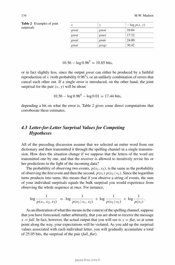
134 M.W. Madsen
Table 2 Examples of jointsurprisals
x y − log p(x, y)
great great 10.84
great graet 17.32
great grate 24.00
great grxqz 30.42
10.56 − log 0.965 = 10.85 bits,
or in fact slightly less, since the output great can either be produced by a faithfulreproduction of x (with probability 0.965), or an unlikely combination of errors thatcancel each other out. If a single error is introduced, on the other hand, the jointsurprisal for the pair (x, y) will be about
10.56 − log 0.964 − log 0.01 = 17.44 bits,
depending a bit on what the error is. Table 2 gives some direct computations thatcorroborate these estimates.
4.3 Letter-for-Letter Surprisal Values for CompetingHypotheses
All of the preceding discussion assume that we selected an entire word from ourdictionary and then transmitted it through the spelling channel in a single transmis-sion. How does the situation change if we suppose that the letters of the word aretransmitted one by one, and that the receiver is allowed to iteratively revise his orher predictions in the light of the incoming data?
The probability of observing two events, p(x1, x2), is the same as the probabilityof observing the first event and then the second, p(x1) p(x2 | x1). Since the logarithmturns products into sums, this means that if you observe a string of events, the sumof your individual surprisals equals the bulk surprisal you would experience fromobserving the whole sequence at once. For instance,
log1
p(x1, x2, x3)= log
1
p(x3 | x1, x2)+ log
1
p(x2 | x1)+ log
1
p(x1).
As an illustration of what this means in the context of the spelling channel, supposethat you have forecasted, rather arbitrarily, that you are about to receive the messagex = fall. In fact, however, the actual output that you will see is y = flat, so at somepoint along the way, your expectations will be violated. As you add up the surprisalvalues associated with each individual letter, you will gradually accumulate a totalof 25.05 bits, the surprisal of the pair (fall, flat).
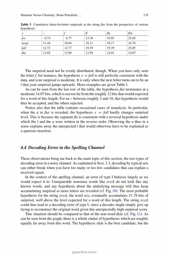
Shannon Versus Chomsky: Brain Potentials … 135
Table 3 Cumulative letter-for-letter surprisals at the string flat from the perspective of varioushypotheses
x – f fl fla flat
for 6.73 6.77 13.38 19.03 25.05
large 11.44 18.04 18.11 18.17 24.78
fall 12.73 12.77 19.39 19.39 25.05
flat 13.85 13.89 13.95 14.01 14.07
The surprisal need not be evenly distributed, though. When you have only seenthe letter f, for instance, the hypothesis x = fall is still perfectly consistent with thedata, and your surprisal is moderate. It is only when the next letter turns out to be anl that your surprisal jumps upwards. More examples are given Table 3.
As can be seen from the last row of the table, the hypothesis flat terminates at amoderate 14.07 bits, which is not too far from the roughly 12 bits that would expectedfor a word of this length. For an ε between roughly 2 and 10, this hypothesis wouldthus be accepted, and the others rejected.
Notice also that the table contains occasional cases of reanalysis. In particular,when the a in flat is revealed, the hypothesis x = fall hardly changes surprisallevel. This is because the segment fla is consistent with a reversal hypothesis underwhich the l and the a were written in the reverse order. Observing the a thus in asense explains away the unexpected l that would otherwise have to be explained asa spurious insertion.
4.4 Decoding Error in the Spelling Channel
These observations bring me back to the main topic of this section, the two types ofdecoding error in a noisy channel. As explained in Sect. 3.3, decoding by typical setscan either break when you have too many or too few candidates that can explain areceived signal.
In the context of the spelling channel, an error of type I behaves largely as wewould expect it to: Unrepairable nonsense words like srxzk do not look like anyknown words, and any hypothesis about the underlying message will thus keepaccumulating surprisal as more letters are revealed (cf. Fig. 10). The most probablehypothesis for the string srxzk, the word size, eventually accumulates 31.78 bits ofsurprisal, well above the level expected for a word of this length. The string srxzkcould thus lead to a decoding error of type I, since a decoder might simply give uptrying to reconstruct the original word given this unexpectedly high surprisal score.
This situation should be compared to that of the non-word flide (cf. Fig. 11). Ascan be seen from the graph, there is a whole clutter of hypotheses which are roughlyequally far away from this word. The hypothesis slide is the best candidate, but the

136 M.W. Madsen
s r x z k
10
20
30
seekspokesizeshesix
Fig. 10 Letter-for-letter surprisal values for various decodings of the string srxzk
f l i d e
15
20
25
slidefridayfliesfled
flight
Fig. 11 Letter-for-letter surprisal values for various decodings of the string flide
difference up to the second best, flies, is only 0.70 bits. For many choices of ε, the twohypotheses slide and flies would thus be simultaneously rejected or simultaneouslyaccepted. Both of those decisions would result in a decoding error.
From the present perspective, it is also interesting that the graph for the varioushypotheses cross each other so frequently: After the fragment fli is presented, the

Shannon Versus Chomsky: Brain Potentials … 137
two hypotheses slide and fled are practically equiprobable. After the fragment flid ispresented, the hypothesis flies is temporarily more probable than the eventual winner,slide. Again, this flip-flopping between roughly equiprobable hypotheses means thata decoder with a not too cautious choice of ε would be in a high danger of committingan error of type II.
This oscillation between competing hypotheses also means that the online decod-ing comes with its own “garden path” phenomenon: Hypotheses with high priorprobability attract early attention which may in retrospect turn out to be unwar-ranted. This is, of course, particularly true if the output word contains errors or isotherwise abnormal so that ordinary expectations do not apply. Regardless of thecause, however, it should be emphasized that this phenomenon occurs here in a sit-uation that does not involve any kind of “syntax” except the possibility of swappingtwo neighboring letters.
We have thus seen two kinds of statistical error related to two kinds of manipulatedstrings. Figuratively speaking, one abruptly pushes the receiver away, while the otherkeeps pushing the receiver back and forth between a portfolio of hypotheses that allseem to fit somewhat, but not quite. The first is associated with errors of type I, andthe other with errors of type II.
5 Discussion
In the previous section, I gave a detailed description of a particular channel modeland the decoding errors that were characteristic of it. This channel took Englishwords as inputs and returned possibly misspelled versions of those strings as outputs.In this section, I will discuss the possibility of designing a similar model that canhandle sentence-level decoding. My conclusion from this discussion is that it involvesadditional hard problems, but that it need not be impossible.
5.1 Two Challenges
I chose to illustrate my hypothesis about the N400 and the P600 by means of thequite simplistic spelling channel because I wanted to sidestep some technical com-plications that were irrelevant to my conceptual point. The word decoding problemis considerably easier than the sentence decoding problem that I really want to study.

138 M.W. Madsen
Two facts in particular make words more manageable than sentences:
1. For most practical purposes, the vocabulary of English can be considered as afinite set, and this means that decoding can be done through exhaustive search.This property sets it apart from many other naturally occurring inference taskswhich have NP-complete decoding problems, such as the most common versionsof statistical machine translation (Knight 1999). Thus, a more realistic modelof the English language would probably require a commitment to a specificsearch heuristic.
2. In spite of half a century of development, we still do not have a good compu-tational theory of English. There is no shortage of formalisms and theories, butanybody who has done any serious attempt to apply these theories beyond a fewtoy sentences will know that we are nowhere near human-level predictive accu-racy. Our language models will thus continue to be a bottleneck in the predictionof psycholinguistic phenomena, since we have no reliable and fully automaticway of computing the conditional probability of a sentence continuation given itscontext (let alone making categorical decisions about “grammaticality”).
Accurate predictions of the occurrence of N400 and P600 effects thus hinge onunsolved and perhaps even unsolvable problems, so perfect prediction is probablyout of the question. However, there is a difference between bad and worse, andgood approximations to English might still capture much of the statistical structurerelevant to the prediction of these phenomena. In the next two subsections, I willgive an example of one possibility for how we can approach the issue.
5.2 A Swap Model and a Trigram Model
Many of the linguistic phenomena associated with the P600 have to do with ordereffects, and it would thus be useful to have a descriptive statistic which measuredto what extent a given English sentence respects the conventional order of wordsin the language. The crudest possible way of quantifying this level of convention-ality is to produce a list of all the word pairs in the sentence, ignoring interveningwords, and then check how frequently those word pairs occur in the same order in areference corpus.
For instance, the sentence There is still time is associated with the pairs
(There, is), (There, still), (There, time), (is, still), (is, time), (still, time).
Using the Brown corpus as a reference, we find that these word pairs occur withthe frequencies
1.1 · 10−5, 5.3 · 10−7, 6.8 · 10−6, 2.9 · 10−6, 7.9 · 10−6, 1.3 · 10−6.

Shannon Versus Chomsky: Brain Potentials … 139
Their corresponding surprisal values are consequently
16.47, 20.86, 17.16, 18.4, 16.95, 19.54.
On average, the surprisal for this string is thus 18.22 bits per word pair, correspond-ing to an “average probability” of 2−18.22 = 3.2 · 10−6 (where the “average” is ageometric average).
This order model captures some long-distance relationships between words, and itcan detect certain fishy-looking word orders. However, it contains no concept of longand short distances, only of “before” and “after.” It consequently has poor grasp ofthe strong, short-distance relations between neighboring words (e.g., the extremelylow probability of the phrase the of ).
These constraints are captured better by a Markov chain model (i.e., a table ofconditional probabilities). Such a model can assign probabilities to the next wordin a sentence given the immediate context, e.g., p(still | There is). Again using theBrown corpus, and assuming a context width of two words, such a model assigns anaverage surprisal of 18.72 bits to the string There is still time. This corresponds to a“average probability” of 2.3 · 10−6.
In this case, the two models thus agree very much in their assessment of the inputstring, but this need not always be the case. In general, it can be advisable to usea mixture of several two complementary models in order to iron out some of theidiosyncrasies that each model has on its own. In the following, I have thus used anequal mixture of the order model and the trigram model, that is, a model of the formp(x) = 0.5 p1(x) + 0.5 p2(x).
5.3 Neighborhood Decoding
An imperfect but very simple decoding method for channels like the spelling channelis to construct the set of source strings that are less than one editing operation awayfrom the observed output, and then find the best candidate in that smaller set.
For instance, for if the output of a spelling channel was y = tup, then the set ofneighboring strings includes
• tip, top, tap, tp, up, tups, tpu, upt, …
and many others. We can then decode y = tup by selecting the x on this list forwhich the joint probability p(x, y) is the highest, hoping that the true solution wasnot more than one operation away. Implementing this decoding algorithm on thesentence level, using no other editing operations than swapping two words, we obtaindecoding candidates such as those shown in Table 4.
As the table shows, even this simple statistical model, which has no conceptof hierarchical structure or syntax, can discover and correct seemingly “high-level”errors. For instance, the decoder correctly pinpoints the words police and prisoner as apotential problem in the first example even though there is no semantic representation

140 M.W. Madsen
Table 4 Potential decodings of an output string
Sentence (y) − 1N log p(y)
The police was trying to escape the prisoner 19.00
The prisoner was trying to escape the police 18.44
I’m afraid so 19.71
I’m so afraid 19.71
The patient looked at his doctor 18.84
The doctor looked at his patient 18.68
The doctor looked at his patient 18.68
The at looked doctor his patient 17.90
The house was parked in front of the car 10.84
The car was parked in front of the house 10.73
The water went straight through the boat 18.14
The boat went straight through the water 17.87
He walked straight to the room of the middle 11.09
He walked straight to the middle of the room 10.45
I heard a flash and saw thunder 19.17
I saw a flash and heard thunder 18.97
The hat put on his man 18.15
The man put on his hat 11.38
The mouse was chasing the cat 20.36
The the was chasing mouse cat 19.20
In each double row, the first sentence is the output string, and the second row is the a posteriorimost probable input sentence that can be obtained by swapping two words. The surprisal values areonly based on the source probabilities, since there is no explicit channel model
whatsoever in the model. In this and several other examples, corrections that seemto require sophisticated knowledge of syntax or semantics are thus achieved on thebasis of nothing but raw word order.
Not all examples are equally convincing, though. The sentence The mouse waschasing the cat is, despite its simplicity, not decoded correctly. A more carefulanalysis of the corpus might reveal why this is the case, but at the time of thiswriting, I have no good explanations.
I should emphasize again here that the decoded sentence in each pair is the singlemost probable sentence in the neighborhood of the output string. The second sentencein each row was identified and selected automatically, based on the probabilitiesassigned by the mixture model. The table should thus not be read as a comparisonbetween two hand-selected sentences.
Notice also that the channel probabilities—that is, the probability of the variousdistortions of a sentence—are not taken into account here; this will make a differenceif these probabilities are very low. The string I’m afraid so will for instance not becorrected to I’m so afraid unless the cost of swapping two neighboring words (interms of surprisal) is practically nil.
Shannon Versus Chomsky: Brain Potentials … 141
5.4 Scaling Up?
The toy model that I have proposed in this subsection is not a perfect model of English,and it could be improved in many ways. I have included it here to indicate that theprinciples discussed in the previous section pertain to any kind of noisy-channelmodel and not just the spelling channel.
Even this very simplistic model, however, was able to detect a number of differentdistortions of a sentence. Many of these distortions and their corresponding correc-tions superficially appeared language-specific or even syntax-specific in nature, butin fact, they were detected and corrected based only on very weak and generalassumptions about the order of tokens in a sequence.
So while the neighborhood decoder for this channel model is quite crude andbrittle, it does demonstrate that there is nothing inherently unrealistic about extendingthe basic statistical idea of this paper to more realistic channel models. Each suchmodel comes with its own version of the two concepts of statistical error, and myclaims about the N400 and the P600 will provide quantitative predictions in eachsuch case—from sentence to sentence, and from word to word. The more difficultpart of the future work thus consists in deciding what kind of channel speech andwriting really is.
6 Conclusion
With the discovery of the P600, it seemed for a while as if the brain sciences hadfound a physiological counterpart of the distinction between semantics and syntax.Over the course of the last decade, this interpretation of the early results has beenconsiderably complicated by further experiments which have produced P600 effectsin a large variety of conditions, many of which are very difficult to explain in termsof syntax as such.
These discoveries have led a number of researchers to stipulate “parallel stream”explanations of the data: For instance, Bornkessel-Schlesewsky and Schlesewsky(2008, p. 67) propose that the P600 occurs when cues from “animacy, voice and otherlanguage-specific information types” clash with the “plausibility” of the assignmentof logical roles that these cues suggest. Kuperberg (2007, p. 44) argues that it is due toconflicts between “a semantic memory-based analysis and possibly a semantically-driven combinatorial thematic analysis.” Kolk et al. (2003, pp. 29–32) suggest thatthe cause is a conflict between an interpretation supported by a “conceptual bias”and another one supported by a “syntactic bias”.
These hypotheses are all very interesting and have a lot of empirical merit. How-ever, I think they are formulated in too linguistic terms and on a too algorithmic level,and hence that they miss the larger conceptual picture. The working philosophy Ihave been applying in this paper is that we should take a principled perspective onthe inference task our subjects are tyring to solve (Anderson 1991). Instead of imme-

142 M.W. Madsen
diately committing to a decoding algorithm in all its gory detail, we should choosea model of the communication situation and analyze its statistical properties beforewe postulate any specific heuristics or neurological implementations. This way, wecan let machinery of statistics decide what counts as a “cue,” a “surprise,” or a “con-flict” instead of inventing a new version of those concepts for every new experiment.This approach will promote models that are more modular, more transparent in theirassumptions, and easier to simulate on individual words or sentences.
To illustrate what this approach entails, this paper has presented a very conven-tional noisy-channel model of spelling mistakes and looked at some of its properties.The decoding problem for this channel was simple enough to be solved by exhaustiveenumeration, and this liberated me to focus on the statistical aspects of the situations.As the example showed, the exhaustive-search decoder for this simple model couldrun into two distinct kinds of statistical error: Words like srxkz produced an excessof surprisal and had no plausible reconstructions, while words like flide had severalcompeting reconstructions, all of which had a surprisal level within the expectedrange. The decoding process could thus derail either because there were too fewplausible decoding hypotheses, or because there were too many.
My claim in this paper is that these two kinds of decoding error—too few and toomany plausible decodings—map onto the N400 and P600, respectively. The P600is thus not produced by a conflict between two “streams” that handle specific typesof information (such as animacy versus word order). Rather, it is caused by moregeneral issues that arise whenever we try to make sense of ambiguous stimuli inan uncertain world. And while it is tempting to describe these issues in a highlytask-specific vocabulary, I would argue that the process of decoding noisy signalsprovides a fruitful framework for understanding N400 and P600 effects.
More broadly, this statistical perspective on reading and listening could have somerather profound consequences for linguistic theory. One of the foundational assump-tions of the Chomskyan program for linguistics is that sentences can be “ungrammat-ical,” a property that can allegedly be separated cleanly from the property of beingnonsensical. From the statistical perspective, by contrast, the notion of “makingsense” would not be assigned to a dark corner, but rather be the centerpiece of thewhole theory. Noisy-channel coding is, at its core, a formalization of the process ofguesswork and sense-making.
These speculations are, however, part of a larger discussion about the foundationsof linguistics that cannot be settled by anything in this paper. I have proposed a specificexplanation of the N400 and P600 effects which made no reference to grammaticaland language-specific concepts, but instead explained these phenomena in statisticalterms. This defuses one of the arguments in favor of linguistic nativism and relatedphilosophical ideas, but it is still an open question how far the style of analysis canbe pushed.
Shannon Versus Chomsky: Brain Potentials … 143
References
Anderson, J. R. (1991). The place of cognitive architectures in a rational analysis. In K. VanLehn(Ed.), Architectures for intelligence (pp. 1–24). New York: Psychology Press.
Bellman, R. (1952). On the theory of dynamic programming. Proceedings of the National Academyof Sciences of the United States of America, 38(8), 716.
Bornkessel-Schlesewsky, I., & Schlesewsky, M. (2008). ProminencePlausibility: An alternativeperspective on semantic P600 effects in language comprehension. Brain Research Reviews, 5(1),55–73.
Chomsky, N. (1957). Syntactic structures. The Hague: Walter de Gruyter.Cover, T. (1975). An achievable rate region for the broadcast channel. IEEE Transactions on Infor-
mation Theory, 21(4), 399–404.Cover, T. M., & Thomas, J. A. (1991). Elements of information theory. New York: Wiley-
Interscience.Damerau, F. J. (1964). A technique for computer detection and correction of spelling errors. Com-
munications of the ACM, 7(3), 171–176.Fernández, E. M., & Cairns, H. S. (2010). Fundamentals of psycholinguistics. Malden: Wiley.Francis, W. N., & Kucera, H. (1967). Computational analysis of present-day American English.
Providence: Brown University Press.Frenzel, S., Schlesewsky, M., & Bornkessel-Schlesewsky, I. (2011). Conflicts in language process-
ing: A new perspective on the N400–P600 distinction. Neuropsychologia, 49(3), 574–579.Gibson, E., Bergen, L., & Piantadosi, S. T. (2013). Rational integration of noisy evidence and
prior semantic expectations in sentence interpretation. Proceedings of the National Academy ofSciences, 110(20), 8051–8056.
Hoeks, J. C. J., Stowe, L. A., & Doedens, G. (2004). Seeing words in context: The interaction oflexical and sentence level information during reading. Cognitive Brain Research, 19(1), 59–73.
Kim, A., & Osterhout, L. (2005). The independence of combinatory semantic processing: Evidencefrom event-related potentials. Journal of Memory and Language, 52(2), 205–225.
Knight, K. (1999). Decoding complexity in word-replacement translation models. ComputationalLinguistics, 25(4), 607–615.
Kolk, H. H. J., Chwilla, D. J., van Herten, M., & Oor, P. J. W. (2003). Structure and limited capacityin verbal working memory: A study with event-related potentials. Brain and Language, 85(1),1–36.
Kuperberg, G. R. (2007). Neural mechanisms of language comprehension. Brain Research, 1146,23–49.
Kuperberg, G. R., Sitnikova, T., Caplan, D., & Holcomb, P. J. (2003). Electrophysiological distinc-tions in processing conceptual relationships within simple sentences. Cognitive Brain Research,17(1), 117–129.
Kutas, M., & Federmeier, K. D. (2011). Thirty years and counting: Finding meaning in the N400component of the event-related brain potential (ERP). Annual Review of Psychology, 62, 621–647.
Kutas, M., & Hillyard, S. A. (1980). Reading senseless sentences: Brain potentials reflect semanticincongruity. Science, 207(4427), 203–205.
Levenshtein, V. I. (1966). Binary codes capable of correcting deletions, insertions and reversals. InSoviet Physics Doklady, 10, 707.
Neyman, J., & Pearson, E. S. (1928). On the use and interpretation of certain test criteria for purposesof statistical inference: Part i. Biometrika, 20A(1/2), 175–240.
Nieuwland, M. S., & Van Berkum, J. J. A. (2005). Testing the limits of the semantic illusionphenomenon: ERPs reveal temporary semantic change deafness in discourse comprehension.Cognitive Brain Research, 24(3), 691–701.
Osterhout, L., & Holcomb, P. J. (1993). Event-related potentials and syntactic anomaly: Evidenceof anomaly detection during the perception of continuous speech. Language and CognitiveProcesses, 8(4), 413–437.

144 M.W. Madsen
Rösler, F., Pütz, P., Friederici, A., & Hahne, A. (1993). Event-related brain potentials while encoun-tering semantic and syntactic constraint violations. Journal of Cognitive Neuroscience, 5(3),345–362.
Samson, E. W. (1951). Fundamental natural concepts of information theory. Technical report E5079, Air Force Cambridge Research Center
Shannon, C. E. (1948). A mathematical theory of communication. Bell System Technical Journal,27, 379–423.
van Herten, M., Kolk, H. H. J., & Chwilla, D. J. (2005). An ERP study of P600 effects elicited bysemantic anomalies. Cognitive Brain Research, 22(2), 241–255.
van Herten, M., Chwilla, D. J., & Kolk, H. H. J. (2006). When heuristics clash with parsing routines:ERP evidence for conflict monitoring in sentence perception. Journal of Cognitive Neuroscience,18(7), 1181–1197.
Viterbi, A. (1967). Error bounds for convolutional codes and an asymptotically optimum decodingalgorithm. IEEE Transactions on Information Theory, 13(2), 260–269.
Weckerly, J., & Kutas, M. (1999). An electrophysiological analysis of animacy effects in the process-ing of object relative sentences. Psychophysiology, 36(5), 559–570.

Orthogonality and Presuppositions:A Bayesian Perspective
Jacques Jayez
Abstract This work focuses on the reasons why the projection properties ofpresuppositional elements are not uniform. Presupposition projection designates thefact that operators that suspend the truth of a proposition have no effect on the pre-supposition it is associated with. For instance, with Paul did not stop smoking, themain content (that Paul does not smoke) is canceled by the negation whereas the pre-supposition that Paul has been smoking is left untouched. It has been observed thatprojection is not uniform across the different expressions that convey a presupposi-tion (its triggers), and a distinction between weak and strong triggers has emerged. Itseems that this distinction correlates with an intuition of (non-)orthogonality, that is,of (non-)independence between the main content and the presupposition. I argue thatthis intuition is correct to some extent but has to be clarified. To this aim, I proposea Bayesian approach, which provides a more precise rendering of orthogonality.
Keywords Presupposition projection · Strong triggers · Bayesian approach ·Bayesian relevance · Layered meaning
1 Introduction
A significant part of the large literature on presuppositions (PP) has been concernedwith the phenomenon of projection. Projection denotes the fact that operators likenegation, interrogation or if, which normally cancel or suspend the truth of a propo-sition, have no effect on the PP associated with the proposition. For instance, inDid Paul stop smoking?, the truth of the proposition that Paul smokes is suspended,whereas the PP that Paul has been smoking remains active. The most natural reading
I am grateful to my two anonymous reviewers for convincing me with excellent arguments torewrite the initial version of this paper. They are not responsible for the remaining shortcomings.
J. Jayez (B)ENS de Lyon and L2C2, CNRS, Lyon, Francee-mail: [email protected]
© Springer International Publishing Switzerland 2015H. Zeevat and H.-C. Schmitz (eds.), Bayesian Natural Language Semanticsand Pragmatics, Language, Cognition, and Mind 2,DOI 10.1007/978-3-319-17064-0_7
145
146 J. Jayez
of the question is ‘Given that Paul has been smoking, is it true or false that he does notsmoke now?’. However, in some cases, the PP itself can be suspended and it seemsthat the possibility of suspending the PP varies with the different expressions thatconvey it (its triggers). Recently, this has led to a distinction between weak triggers(or soft triggers), those that allow for suspending the PP, and strong triggers (or hardtriggers), which do not. Although this distinction has some empirical support, it isfar from transparent. Why should some triggers be ‘stronger’ than others? It seemsthat the difference depends on the (degree of) orthogonality of the PP and the maincontent (MC). For instance, in Paul stopped smoking, the MC (Paul does not smoke)and the PP (he has been smoking) seem to be somehow ‘entangled’, whereas withPaul hit the target too, the MC (Paul hit the target) and the PP (someone else did)seem to be independent (‘orthogonal’). In this paper, I show that orthogonality is notexactly what we need and that the difference between weak and strong triggers isamenable to a general principle regulating discourse attachment in a Bayesian frame-work. In Sect. 2, I recall the main notions and observations that are at the origin of theprojection problem. In Sect. 3, I present introspective (Sect. 3.2) and experimental(Sect. 3.3) data that seem to support the distinction betweenweak and strong triggers.I discuss the interpretation of the experimental data in Sect. 3.4, arguing that they areactually based on a metalinguistic interpretation. I turn to orthogonality in Sect. 4.In Sect. 4.1, I present Abbott’s take on the weak/strong distinction and argues thather analysis in terms of detachability is misleading. However, I defend her intuitionin Sect. 4.2 and show how it can be expressed in a Bayesian framework. Finally, inSect. 5, I address two remaining problems. Admittedly, the empirical scope of thispaper is limited because I do not study the full range of triggers (see Sect. 3.1 for adiscussion of this problem). However, one has to start somewhere and I think that isnot inconsequential to show that the distinction between weak and strong triggers,which has gained great currency in semantics, has to be reanalyzed.
2 Presuppositions and Projection
2.1 Basic Notions
Natural languages offer to speakers the opportunity to convey different types ofinformation in a single utterance. The MC concerns the most basic truth-conditionalcontribution of the utterance, whereas the non-MCconcerns, for instance, intellectualor emotional attitudes of the speaker, or what she presupposes to be true. So, (1a)informs the hearer that some friend of the speaker found a solution (MC), but alsothat this fact was unexpected (intellectual attitude) and that the speaker does not holdthe mentioned friend in high regard (emotional attitude). (1b) asserts that Charleshas talked to someone (MC) and presupposes that it is his sister.
(1) a. Unexpectedly, my stupid friend found the solution.b. Charles has talked to his sister.
Orthogonality and Presuppositions: A Bayesian Perspective 147
A quick test to separate MC and non-MC is to consider what the natural target ofa direct refutation is. In most cases, people interpret the target as being the MC, see(2) and (3).
(2) A—Unexpectedly, my stupid friend found the solution.B—It’s false/You’re wrong/You’re mistaken.
� Your friend did not find the solution�� It’s not unexpected or/and your friend is not stupid
(3) A—Charles has talked to his sister.B—It’s false/You’re wrong/You’re mistaken.
� Charles did not talk to his sister�� Charles has no sister
Among the expressions conveying a non-MC, presuppositions (PP) have beenthe subject of intensive research. Intuitively, a PP is a piece of information whichis taken for granted or presented as such (Stalnaker 1974) or must be true in everycontextwhere the sentence conveying it canbe assertedwithout contradiction (Beaver2001; Heim 1983). A hallmark of the non-MC is its tendency to project, that is, toremain unaffected by operators that negate or suspend the MC, such as negation,interrogation or if. For instance, whereas the proposition that my friend found thesolution does not receive a definite truth-value in (4), the non-MC (my friend isstupid) is endorsed by the speaker exactly as in (1a). A similar difference holds fornegation and conditional.
(4) Did my stupid friend find the solution?�� My friend found the solution� My friend is stupid
2.2 Ideal and Actual Projection
In an ideally simple world, projection would be uniform across all types of triggers.What is the situation in the real world? Non-MC tends to project rather neatly forconventional implicatures (Potts 2005) such as evaluative adverbs (unexpectedly) orexpressives (Determiner + stupid + N, interjections, etc.). What happens for PP?There is clearly a tendency to project, see Chierchia and McConnell-Ginet (1990),Geurts (1999), Beaver and Geurts (2013) for different surveys. For instance, there isa strong intuition that all the forms in (5) presuppose that Paul has been smoking.
(5) a. Paul stopped smoking.b. Paul didn’t stop smoking.c. Did Paul stop smoking?d. It is possible that Paul stopped smoking.e. If Paul stopped smoking, he must feel better.

148 J. Jayez
Concerning the difference with conventional implicatures, conditional structuresthat suspend a PP seem to have no effect on implicatures, as suggested by the differ-ence between (6a) and (6b), which sounds odd or heavily metalinguistic.
(6) a. If Paul has been smoking, he has stopped.�� Paul has been smoking
b. ? If my friend is stupid, then my stupid friend found the solution.
However, this is not true for every type of conventional implicature, in particularfor appositive relatives, see (7). In a context where Paul is John’s friend, the speakerdoes not necessarily endorse the view that Paul is stupid.
(7) If Paul is stupid, John can expect that his friend, who is not very clever,won’t find the solution.
If projection for PP was uniform, the difference between conventional implica-tures and PP would be essentially a matter of domain. For instance, conventionalimplicatures could perhaps be conceived as concerning all the domains where evalu-ation, whether emotional or intellectual, plays a central role. However, it seems that,whereas implicatures project in a systematicway, it is not the case for PP. For instance,Karttunen (1971) introduced a difference between full factives like regret, whose PPalways project, and semi-factives like discover, whose PP may be suspended, as in(8). See Beaver (2004) for a thorough discussion.
(8) a. If I discover that I was mistaken, I will admit publicly I was wrong.�� I was mistaken
b. If I regret that I was mistaken, I will admit publicly I was wrong.� I was mistaken
Other ways to suspend the PP include the following ones.
1. Ignorance about the PP (Geurts 1995), as in (9).2. Negation of the PP in answers (Cummins et al. 2013), as in (10), where the A1-B1
exchange is judged by speakers to be better than the A2-B2 exchange.3. Abusch (2002, 2010) suspension test, as in (11)
(9) [Context: Paul has never seen or heard about Mary smoking, but she seems verynervous and restless. He wonders whether Mary has been smoking and is tryingto stop.]Is Mary quitting smoking?�� Mary has been smoking
(10) A1—Has John stopped smoking?B1—No, because he never smoked before.A2—Has John smoked again?B2—No, because he never smoked before.

Orthogonality and Presuppositions: A Bayesian Perspective 149
(11) a. I have no idea whether Paul participated in the Road Race yesterday.But if he won it, then he has more victories than anyone else in history.(=Abusch’s 2010 example 3d)
b. ?? I don’t know if Paul participated in the race, but if Mary participatedtoo, they probably ran together.
These and similar examples suggest that (i) PP projection has a certain degree ofvariability and (ii) that it is probably not just a matter of context or pragmatic consid-erations. Stalnaker (1974) defended the idea that projection is a default or preferredbehavior, which can be more or less plausible in different contexts. For instance, heexplained the non-projection in (8a) by noting that, if the speaker of (8a) presupposesthat she has missed the point, she necessarily realizes that she did so. So, by contra-position, if she does not realizes she has missed the point, she cannot presuppose thatshe did, hence the lack of commitment to the PP (absence of projection). So, a simplereasoning about the plausibility of the PP leads to abandoning it. Unfortunately, itis difficult to understand along the same lines the difference between too or again,which are robustly projective, and stop or win, for which the PP can be suspendedmore easily.
3 Weak and Strong Triggers
Examples (10) and (11) suggest that there at least two classes of triggers. Strong trig-gers (ST) always give rise to projection whereas weak triggers don’t. This distinctionis supported both by introspective and experimental data. Before presenting thesedata, however, I need to clarify what the ambition and limits of trigger taxonomiescan be. This is done in the next section.
3.1 A Disclaimer in Form of Clarification
In the previous section I have mentioned some well-known cases. A reviewer com-plains that I have confined my attention in this paper to “a rather limited numberof presupposition triggers”. This is quite true but can hardly be avoided. First, asevidenced by the (partial) list in Beaver and Geurts (2013), there is a huge set ofpresumed PP triggers. The goal of the present paper is not to study the variabilityof triggers per se but only with respect to projection. There are a lot of important orminute differences that are not captured by a distinction in terms of projection and Idid not intend to address them for a simple reason: I am unable to offer a ‘complete’theory of PP triggers, meaning a theory in which each trigger would be describedcompletely and correctly. I suspect that such a theory would require a detailed lex-ical analysis of each trigger. I am not aware of the existence of such a theory in theliterature and I do not feel committed to proposing one.

150 J. Jayez
Second, it is almost impossible to have clear-cut introspective intuitions on a verywide range of PP triggers, and it might be impossible to have clear intuitions on sometriggers except in well-known (and generally trivial) cases. The strategy of the paperis, accordingly, to focus on a number of items that are considered as representativeof some major categories: aspectual verbs like begin, emotive factives like regret,clefts, ‘strong’ adverbial triggers like too. Although their number is indeed limited,they span a not insignificant number of categories of PP triggers. I assume that thecategories addressed in the paper are sufficiently interesting to be worth studying(I might be wrong).
My proposal is based to a large extent on experimental observations. The interestof an experimental approach is twofold. First, by going beyond the intuitions ofisolated speakers, there is more chance to detect general tendencies, if any, and tocompensate for the variability of introspective judgments. Second, an experimentalperspective forces one to remain aware of the limits of large scale comparisons.Measuring the ‘projectability’ of triggers with comparison tests raises the questionof the interpretation context. When we are given sentences in isolation or with avery limited or very specific context, we are not necessarily able to quickly scana sufficiently large set of contexts in order to find a ‘good’ one, that is, a contextthat makes the sentence natural. So, a naturalness signal1 can reflect the degreeof context accessibility/construction. To use a generic term, I will call the task ofinferring a context that makes a linguistic stimulus plausible context abduction. Tomy best knowledge, there is at the moment no established technique for measuringcontext abduction.However,when a context can be providedwhichmakes a linguisticstimulus natural, whereas the same stimulus is massively perceived as not naturalin isolation, one can reasonably suppose that the licensing context cannot be easilyabduced. This is the main idea behind the experiment reported in Sect. 5.2. There,two triggers considered as strong are considered, regret and clefts. It is shown that, insuitable contexts, the PPof these triggers can be explicitly suspendedwithout creatingan impression of contradiction (it does not project). However, the contexts that makenon-projection possible are not the same for the two triggers. Therefore, comparingthe two triggers would be more risky because it would amount to comparing thebehavior of two items in different contexts.Clearly, this is a general problem.SincePPtriggers are very different, it is difficult and perhaps impossible to show in a rigorousway how exactly they compare to each other in terms of degree of projection. It isfor instance possible that triggers that allow non-projection and are thereby similardiffer nonetheless in terms of degree of projection strength but that the differenceis impossible to evaluate. Once the context is given, this possible difference mightdisappear. When isolated sentences are considered, observed differences might beattributed to context abduction rather that resistance to projection. If the samecontextscould be used, we would of course be in a better position to adopt a truly comparativeperspective.
1Whether this signal is an explicit judgment or a different manifestation such as a reading time,fixation or ERP measure does not change the basic problem.

Orthogonality and Presuppositions: A Bayesian Perspective 151
The upshot of these remarks is that, whereas it would be extremely interesting tocompare triggers pairwise, it is also a difficult task, which seems to be beyond ourreach for the time being.
3.2 Introspective Data
The idea that PP triggers differ in their projection behavior is mentioned in severalplaces in the linguistic and philosophical literature on PP. However, there is in generalno systematic attempt to lay the foundations of a classification. Three notable excep-tions are Abbott (2006), Abusch (2002, 2010) and Zeevat (1992). Zeevat’s proposalis discussed in Sect. 3.3. Its relation to the WT/ST distinction is less clear than in theworks of Abbott and Abusch, which also offer the advantage of capitalizing on morerecent contributions. In this section, I adopt Abbott’s and Abusch’s point of view andfocus on the three main points that are to be found in their papers.
First, Horn (1972) identified a possibility of suspending a PP bymeans of a specialif -clause or a may not construction (12a). According to him, the first sentence mustbe negative (12b)
(12) a. John does not realize that Sue loves him, if indeed she does.b. # If John realizes that Sue loves him (and in fact she may not), thenhe’ll tell us.
One can observe that regret or again, for instance, are less felicitous in environ-ments comparable to (12a).
(13) a. ? John does not regret that Sue loves him, if indeed she does.b. ? John has not studied the problem again, if indeed he has studied it before.
Second, there is the discover/regret contrast mentioned by Karttunen, whoseexamples can be adapted to avoid the first-person effect mentioned by Stalnaker (seeBeaver (2004)). Various similar observations suggest that epistemic factives like dis-cover or know are WT, whereas emotive factives like regret or be glad/sad/happy/surprised are ST.
(14) a. If someone discovers that I was mistaken, I will admit publicly I was wrong.�� the speaker was mistaken
b. If someone regrets that I was mistaken, I will admit publicly I was wrong.� the speaker was mistaken
Finally, there is Abusch’s test, used in (11). The structure of the test sentencesis: ?p′, but if p, q, where p presupposes p′. What is tested is the possibility ofaccommodating the missing PP (whose truth has been suspended by a preliminaryignorance statement) in the local context corresponding to the antecedent of the ifp, q conditional.
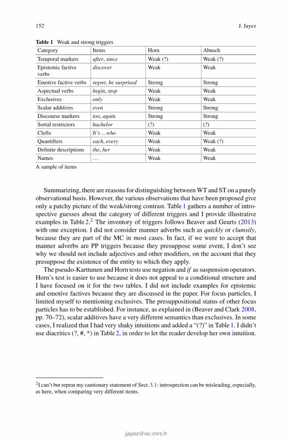
152 J. Jayez
Table 1 Weak and strong triggers
Category Items Horn Abusch
Temporal markers after, since Weak (?) Weak (?)
Epistemic factiveverbs
discover Weak Weak
Emotive factive verbs regret, be surprised Strong Strong
Aspectual verbs begin, stop Weak Weak
Exclusives only Weak Weak
Scalar additives even Strong Strong
Discourse markers too, again Strong Strong
Sortal restrictors bachelor (?) (?)
Clefts It’s …who Weak Weak
Quantifiers each, every Weak Weak (?)
Definite descriptions the, her Weak Weak
Names … Weak Weak
A sample of items
Summarizing, there are reasons for distinguishing betweenWTandSTon a purelyobservational basis. However, the various observations that have been proposed giveonly a patchy picture of the weak/strong contrast. Table1 gathers a number of intro-spective guesses about the category of different triggers and I provide illustrativeexamples in Table2.2 The inventory of triggers follows Beaver and Geurts (2013)with one exception. I did not consider manner adverbs such as quickly or clumsily,because they are part of the MC in most cases. In fact, if we were to accept thatmanner adverbs are PP triggers because they presuppose some event, I don’t seewhy we should not include adjectives and other modifiers, on the account that theypresuppose the existence of the entity to which they apply.
The pseudo-Karttunen andHorn tests use negation and if as suspension operators.Horn’s test is easier to use because it does not appeal to a conditional structure andI have focused on it for the two tables. I did not include examples for epistemicand emotive factives because they are discussed in the paper. For focus particles, Ilimited myself to mentioning exclusives. The presuppositional status of other focusparticles has to be established. For instance, as explained in (Beaver and Clark 2008,pp. 70–72), scalar additives have a very different semantics than exclusives. In somecases, I realized that I had very shaky intuitions and added a “(?)” in Table1. I didn’tuse diacritics (?, #, *) in Table2, in order to let the reader develop her own intuition.
2I can’t but repeat my cautionary statement of Sect. 3.1: introspection can be misleading, especially,as here, when comparing very different items.

Orthogonality and Presuppositions: A Bayesian Perspective 153
Table 2 Weak and strong triggers. Examples of use
Category Test type Example
Temporalmarkers
Horn Paul didn’t change his mind since he read the review, if indeedhe read it
Abusch I don’t know whether Paul read the review, but, if he changedhis mind since, the final version of the paper is going to bepretty different
Aspectual verbs Horn Paul has not stopped smoking, if indeed he has been smoking
Abusch I don’t know whether the victim has been smoking before, but, ifhe has stopped smoking, we should find traces of tobacco tar inhis lungs
Exclusives Horn I doubt that only Paul came, if indeed he came
Abusch I don’t know whether Paul came, but, if only him came, it musthave been disappointing
Scalar additives Horn I doubt that even Paul missed the target, if indeed it would beTHAT surprising
Abusch I don’t know whether Paul missing the target would be verysurprising, but, if even him missed the target, we’ll see what theothers will do
Discoursemarkers
Horn I doubt that Paul missed the target again, if indeed he missed itbefore
Abusch I don’t know whether Paul missed the target before, but, if hemissed it again, really, it’s a pity
Sortal restrictors Horn This Jordan is not a bachelor, it seems, if indeed Jordan is amale
Abusch I don’t know whether this super rich Jordan is a male, but if heis a bachelor, he certainly has a lot of women chasing after him
Clefts Horn It’s not Paul who solved the problem, if indeed someone solvedit
Abusch I don’t know whether someone solved the problem, but, if it’sPaul, he must be very proud
Quantifiers Horn Since he settled only very recently, I doubt that everyprofessional nurse in the town met the new doctor, if indeedthere are professional nurses in such a little town
Abusch I don’t know if any student cheated, but, if every student whocheated has been expelled, we’ll see if some students aremissing at the beginning of the next term
Definitedescriptions
Horn Paul didn’t find the key, if indeed there is a key for this door
Abusch I don’t know if there is a key for this door, but, if Paul found thekey, we are lost
Names Horn I never met this Mr Slush, if indeed there is someone with thisname
Abusch I don’t know whether there is a Mr Slush, but, if Dora met himshe is in trouble

154 J. Jayez
3.3 Experimental Data
Certain–but not all–introspective observations are confirmed by the experimentreported in (Cummins et al. 2013). Cummins et al. draw their initial motivation fromZeevat’s (1992) distinction between three different types of triggers, a distinctionwhich I summarize in the next paragraph.
Resolution triggers form the first category. They are strongly anaphoric, that is,they demand that the entities they refer to be present in the environment (discourse orsituation) at themoment the PP trigger is used. Zeevat mentions definite descriptions,when- and after-clauses, as well as–tentatively–clefts. Lexical triggers correspond to“concepts with the applicability conditions”, which means that certain conditions–corresponding to the PP–must be met for the concept to be applicable. An exampleprovided by Zeevat is regret. At this stage, there is a significant complication. Zeevatassumes that a trigger can trigger several PP. For lexical triggers like verbs and nouns,the sortal information–whether we refer to an event or to an individual–is lexical innature, whereas the descriptive information–what is predicated of the event or theindividual-can be resolutive. For instance, Zeevat analyses an example like Johnbelieves that the king is bald as divided into a lexical presupposition, a resolutionpresupposition and a content (the MC of the present paper), see (15).
(15) John believes that the king is bald.Lexical PP : x (x has the type of individuals)Resolution PP: x ∧ king(x)
Content : B j bald(x)
Zeevat also considers triggers like again, also, another and too. They are charac-terized by their ability to involve parts of the context that are not normally accessible,as illustrated by (16).
(16) John believes that Mary was in Egypt. Sue was there too
Cummins et al. intend to compare the experimental correlates of lexical and res-olution triggers. In fact, the set of triggers they choose contains (i) lexical triggers(regret, continue, stop), only, and comparatives, (ii) two triggers of the third type(again and too) and (iii) still. This is a little confusing but I assume that their goalis essentially to compare triggers which look for an antecedent (again, too and still)and triggers which express their PP directly in their lexical content. I will call theformer anaphoric and the latter lexical. Concerning comparatives, I am skeptical asto their presuppositional status, since the alleged PP is not robust in a plain assertion:Mary is more clever than Paul, who is really rather stupid.
In their main experiment, Cummins et al. use an evaluation task where subjectshave to rate some dialogs on a 5-point scale. The distribution of possibilities is asfollows, for the trigger again.3
3As noted by a reviewer, the bottom right case is not very clear. The answer No, because he didn’tlose his wallet before could be interpreted as Endorsing MC + Refuting PP. I won’t try to take this

Orthogonality and Presuppositions: A Bayesian Perspective 155
Fig. 1 Results of the second Cummins et al. experiment
The initial expectations of the authors are that the combination of endorsing theMC and refuting the PP are better for anaphoric triggers than for lexical triggersand that the combination of refuting the MC and the PP is better for lexical triggersthan for anaphoric triggers. The results are summarized in Fig. 1. The stars indicatesignificance in the difference between the scores for the No, because … (left bar) andYes, although … (right bar) answers.
Based on the introspective data of the previous section, one would expect thatregret, continue, stop and only are WT, whereas still,4 again and too are ST. Asindicated, I leave aside the case of comparatives. There is no significant differencefor again and too, but they don’t pattern alike. Still does not align with too andagain, although it is considered to be a ST. Similarly, there is a difference for the(presumably) ST regret. So, the results delivered by the experiment do not coincidewith introspection and call for an analysis of the task itself.
The main question that experiments of this type raise is to determine how thesubjects interpret the dialogs they have to evaluate. Consider a set of pairs like thosein Table3. When a subject sees the answer Yes, although he didn’t lose his walletbefore, what does she understand? It seems pretty obvious that the answerer meansthat she considers the proposition that Brian lost his wallet as true. But what is themeaning of although? It is unlikely that although signals an incompatibility betweenthe fact of losing one’s wallet and the proposition that one has not lost one’s walletbefore, because such a connection would be very obscure. It is likely, in contrast,
(Footnote 3 continued)interpretation into account, but its existence is an additional symptomof the difficulty of determiningwhat the target of Yes/No and although/because is exactly in this type of experiment.4In my intuition, still does not behave differently from too or again with respect to the Horn andAbusch tests.

156 J. Jayez
Table 3 The four possibilities in Cummins et al. design
that although is ‘metalinguistic’, that is, it indicates that the answerer has not usedan appropriate expression. Is it also the case with because in other examples? Whatare the most reasonable predictions one can make, given the interpretations assignedto the different micro-dialogs presented in the experiment? Do these predictionscorrespond to what is observed by the authors? In the next section, I try to clarify theimport of Cummins et al. experiment, before reconsidering the WT/ST distinctionin the light of introspective and experimental observations in Sects. 4 and 5.
3.4 Discussion of the Experiment
Let us suppose that the yes and no particles in the various answers are free to tar-get the MC alone, the PP alone or the MC+PP combination. I will call this set ofconfigurations the free attachment scenario. Under this scenario, there is no a prioriplausibility in favor of one specific attachment, in comparison to the others. Clearly,this scenario is only a theoretical and rather implausible possibility. Nevertheless, itis useful to enumerate all the possibilities and sort out those that stand a chance.
Figure2 shows the different possibilities of the free attachment scenario. Table4compares what is predicted under the free attachment scenario to what is observedby Cummins et al.
Let us first describe the predictions of Table4. With Yes-1, that is, when Yestargets the MC alone, we predict that the perceived quality of the Yes, although …answer should depend on the interpretation of the although discourse marker. If
Fig. 2 The a prioripossibilities for attachment
MC PP
Yes
MC PP
1 2
3
MC PP
No
MC PP
1 2
3

Orthogonality and Presuppositions: A Bayesian Perspective 157
Table 4 Predictions and observations
Category Diagnostic Prediction for ST andWT
Observed
Yes-1 Depends on although WT = ST WT �= ST
Yes-2 Contradictory (PP andnot PP)
WT = ST WT �= ST
Yes-3 Contradictory (PP andnot PP)
WT = ST WT �= ST
No-1 Explanation relationobscure
WT = ST WT �= ST
No-2 Redundantexplanation (Xbecause X)
WT = ST WT �= ST
No-3 ?OK WT = ST WT �= ST
it is interpreted as introducing only a correction, the answer should be judged ascorrect because its meaning can be paraphrased by “what you sayMC is true, but yourquestion presupposes something which is false”. Although might also be interpretedas introducing an opposition. In that case, a form ‘A although B’ would mean ‘A istrue but B, others things being equal, makes the probability of A decrease’. Underthe opposition interpretation, the negation of the PP would be seen as making theprobability of the MC decrease. It is not clear that this interpretation correspondsto our intuition in the general case. However, we might imagine contexts in whichthis dependency holds. For example, sailing across the Atlantic (as a pilot) probablydemands some experience. So, one might think that, if you never crossed the Atlanticbefore and if you are not an experienced sailor, it is rather unlikely that you cansucceed. If Paul is an unexperienced sailor, one might imagine a dialog like (17).In the case of (17), B’s answer should sound natural, since it means something like“Yes, he has crossed the Atlantic, although it was his first experience”.
(17) A—Has Paul crossed the Atlantic again?B—Yes, although he never crossed it before.
Whatever the interpretation for although is, the prediction for an exclusive MCattachment is that ST and WT should not be different. Let us review more briefly theother attachment configurations. For Yes-2, the target of the answer is the PP, whichmakes the answer self-defeating, since the PP is endorsed and rejected at the sametime. A similar diagnosis has to be made for Yes-3, where the MC and the PP are thetargets. In the latter two cases, no difference between ST and WT is predicted. Allin all, for Yes, the free attachment scenario does not predict any difference betweenWT and ST.
With No-1, the answer presents the negation of the PP as a reason to believe thatthe MC is false. The causal relation behind this reasoning is rather obscure in thegeneral case. It might perhaps be clearer in particular contexts, like with although in
158 J. Jayez
the case of Yes-1. With No-2 (the PP is the target), because introduces a redundantexplanation (¬p because ¬p). The last case might be more felicitous. No targets theMC and the PP and the answer might be interpreted as ‘it is not true that AMC andBPP because it is not true that BPP’. Under the three No versions, like in the caseof Yes, the free attachment scenario does not predict any difference between WTand ST.
What are the observations? Generally speaking, the predictions of the abstracttheory (free attachment) are not borne out. There are differences between triggers.How can we make sense of what Cummins et al. observe? The authors report twodifferent findings. First the Yes, although … answer is judged to be globally worsethan the No, because … one. This can be explained straightforwardly if we assumethat the answers target the conjunction of the MC and the PP. In that case, Yes,although … is predicted to be anomalous for reasons we just saw with the commentof Yes-3 in Table4. The speaker endorses A and B and rejects B immediately after,which is a plain contradiction.
The second finding is the difference between WT and ST–or, more precisely,between certain items classified as ST and certain items classified as ST. Unfortu-nately, it turns out that the results of the experiment are difficult to interpret, giventhat there is a potential confound created by because. Under a descriptive (causalor logical) interpretation, ‘A because B’ presents B as a cause of or a reason for A.Under a metalinguistic interpretation, ‘A because B’, where A has a negative form¬C , presents B as a reason for not using the form of words associated with C.
Horn (2001, Chap.6) exposes all the intricacies of metalinguistic negation. Thetype ofmetalinguistic interpretation that is relevant in the context of the present papercan be described as in (18).
(18) A metalinguistic interpretation consists in assuming the existence of an even-tuality while denying that it can be described correctly by a certain form ofwords.
To illustrate, consider (19). B1’s answer is a plain negative answer. There was noevent of Paul tidying up his room. This answer does not commit B1 to somethinghappening at all. For all we know, Paul might have stayed quietly in his armchair.B2’s answer, where the first syllable of tidy up is stressed, conveys the idea thatsomething happened which cannot be properly called tidying up. It is well-knownthat marking focus with a stress, as here, is conducive to a contrast interpretation,in which several alternatives are competing (Beaver and Clark 2008; Erteschik-Shir2007; Rooth 1992).
(19) A—Did Paul tidy up his room?B1—He didn’t.B2—He didn’t TIdy up his room.
In our case, the relation between the metalinguistic interpretation and the PP isrelatively clear: the failure of the PP makes its trigger linguistically inappropriate.Note, however, that a metalinguistic interpretation can make use of the MC. For
Orthogonality and Presuppositions: A Bayesian Perspective 159
instance, in (20), B underlines the fact that the MC (Paul does not smoke) is not anexact description of the actual situation, although it bears some resemblance to it.
(20) A—Paul stop smoking?B—He didn’t STOP, but he is smoking less and less.
In order to interpret some of the results of the Cummins et al. experiment, onehas to determine, as far as possible, whether the subjects see certain dialogs with aNo, because … answer as metalinguistic or descriptive. I won’t consider the MC-addressing metalinguistic interpretations in discussing Cummins et al. experiment,because it is clear that the MC is not directly rejected in the No, because … answers.Consider dialog (21). A MC-addressing metalinguistic interpretation would amountto paraphrasing B’s answer by ‘It is not appropriate to say that Brian lost his walletbecause he did not lose it before’, which hardly makes sense.
(21) A—Did Brian lose his wallet again?B—No, because he did not lose his wallet before.
However, the MC might be indirectly affected by the rejection of the PP, and Iwill have to take this possibility into account. It corresponds to what I have calledthe descriptive interpretation, in which negating the PP of the question (‘Brian didnot lose his wallet before’) could make the probability of the negation of the MC(‘Brian did not lose his wallet’) increase.
How could we discriminate between the descriptive and the (PP-addressing) met-alinguistic interpretation in our case? If the interpretation is descriptive, we have twopossibilities. (i) The negation of the MC is caused or justified by the PP. This is veryimplausible in the general case. For instance, the No, because … answer to a testsentence like Did Ben regret arguing with his boss? would be interpreted as “Benhas no negative feeling about arguing with his boss because he didn’t argue withhis boss”. If this paraphrase means that Ben does not regret having argued with hisboss because he didn’t argue, what is explained or justified is not, in fact, the MCalone but the MC+PP compound. If the paraphrase means that Ben has no negativefeelings with the very idea of arguing with his boss because that did not happen, themeaning is at best unclear since the descriptive (causal/logical) link is not particu-larly obvious. More importantly, interpreting the No, because … answer as a ‘¬MCbecause ¬PP’ pattern, is counterintuitive. If it was a natural answer, the followingdialog should sound felicitous, which is not the case.
(22) A—Did Ben regret arguing with his boss?B—Ben has no problem with the idea because he didn’t argue with his boss.
(ii) The second possibility for the descriptive interpretation is that theNo, because… answer rejects a logical and-conjunction because one of its terms is false. Forinstance, the following dialog (23) would receive the interpretation in (24). Similarly,the answer on the MC would correspond to (25).
(23) A—Does Toby continue to watch films?B—No, because he didn’t watch films before.

160 J. Jayez
(24) A—Does Toby watch films and did he watch films before?B—No, because he didn’t watch films before.
(25) A—Does Toby watch films and did he watch films before?B—No, because he does not watch films.
Given (24) and (25), onewould not expectmuch difference between aNo, becauseanswer refuting the PP (24) and a No, because … answer refuting theMC (25). Thisis precisely what we don’t observe. In a first experiment, Cummins et al. (2013) showvery clearly that speakers prefer an attachment to the MC, which echoes previoussimilar experimental findings in (Jayez 2010).
Summarizing, the most plausible candidate for the No, because … answer is thePP-addressing metalinguistic interpretation, where a speaker underlines the inappro-priateness of a linguistic form by denying the PP it triggers. Moreover, this interpre-tation is expected to remain rather marginal, because it creates a garden-path effect.The No, because part triggers an expectation that the answerer addresses the MC(descriptive interpretation) whereas the rest of the sequence only makes sense undera metalinguistic interpretation. Given that both Yes, although … and No, because… answers are most naturally interpreted as metalinguistic, we can account for theobserved difference between the scores for the Yes, although … and the No, because… answers. Moreover, we expect that, when the PP is difficult to suspend (ST),even the Yes, although … answer will not be perceived as natural, so the differencebetween the Yes, although … and the No, because … will be smaller than when thePP is easier to suspend (WT).
We can conclude that Cummins et al. experiment confirms that there exists adifference in the robustness of the PP, in agreement with the general feeling thatsome triggers (the ST) are more robust than others (the WT). However, the resultsleave us with two questions.
(1) The correspondence with the introspective data is imperfect. First, still and regretseem to be ST, whereas the experiment classifies them as WT. Second, the reasonwhy again and too have inverse profiles is unclear, even if the difference betweenthe scores for the two answer types is not significant. Third, how is it that too hasa markedly better score for the Yes, although … answer than regret, only, continueor stop?(2) The nature of the distinction between WT and ST remains a bit mysterious.Clearly, not all triggers behave the same. Is this sufficient to conclude that they fallinto ‘natural’ classes, e.g. anaphoric versus lexical or strong versus weak? Shouldthe difference be conceived instead on an item-per-item basis, or should we consideran intermediate taxonomy, with several small classes, possibly originating from a setof parameters?

Orthogonality and Presuppositions: A Bayesian Perspective 161
4 Separation and M-Relevance
4.1 Abbott on Detachability
Abbott (2006) offers a precious cue. She notes an apparent correlation betweenthe status of triggers and the relation between MC and PP. The PP of ST corre-spond to pieces of information which are orthogonal to the MC, as evidenced bythe nondetachability criterion, in the sense of (Grice 1989, Chaps. 1–2). Grice dis-cusses nondetachability in the context of conversational implicatures. A conversa-tional implicature is non detachable whenever it is not possible to ‘say’ the samething, that is, to convey the same MC, without triggering the same conversationalimplicature, unless some feature of the alternative expression is relevant to the deter-mination of the original implicature. Conversational implicatures are in general (butnot always) nondetachable, whereas conventional implicatures are in general detach-able. Interestingly, (Grice 1989, p. 43) mentions the implicatures of PP triggers asnondetachable. In Paul stopped smoking, the proposition that Paul has been smokingwill survive any attempt to reformulate ‘what is said’ in Grice’s sense.
Let us assume for the moment that Grice is right. Clearly, with ST, it is possible to‘say’ the same thingwithout the PP. So STwould be analogous to conventional impli-catures, which, moreover, are reputedly hard to suspend (Potts 2005), like ST. Abbottexplains the common resistance of ST and conventional implicatures to suspensionby resorting to a mechanism of intention attribution. A speaker has a choice betweencommunicating the PP of a ST or not. Since the PP and the MC are informationallyindependent, and the speaker chose to communicate the PP, the latter must be part ofher communicative intention. For instance, in using Mary hit the target again insteadof Mary hit the target, a speaker lets us think that drawing our attention to the PP isan essential part of her message, hence the incompatibility with suspension, whichwould result into an incoherent conversational plan.
It seems that Abbott’s account suffers from the same problem as Grice’s. It isjust technically incorrect to claim that PP of verbs like stop, or of WT in general,are nondetachable. There are perfectly good ways to ‘say’ the same thing withoutconveying the same PP. First, there is the possibility of asserting the MC alone, likePaul does not smoke with respect to Paul stopped smoking. One might object that,when using Paul does not smoke, we do not convey the same content because thetransition from an activity of smoking to its negation gets lost. At the root of thisobjection, there is a frequent cognitive illusion about the MC. A plausible logicalformula corresponding to Paul stopped smoking is shown in (26.2). t is a time point(or a small incompressible time interval), I1 and I2 are time intervals, � (�) are therelations of right- (left)-abutting. t � I iff t (or its smallest upper bound, if t is aninterval) is the greatest lower bound of I . I � t is defined symmetrically. (26.2) saysthat there is a past time t such that Paul has been smoking just before t and didn’tsmoke for some time just after t . The MC is shown in (26.3). It says that John didn’tsmoke for some time, just after some time t . We might express the MC simply bysaying Paul didn’t smoke or Paul has not been smoking, or, if we are sure that Paul
162 J. Jayez
didn’t start smoking again, by Paul does not smoke. Admittedly, we do not therebyconvey the same information as with Paul stopped smoking, but the information welose depends on the PP, not on the MC. We are just asserting that there is some pasttime point after which Paul didn’t smoke, during some time interval which extendsor not to the present, and this is indeed the ‘substance’ of the MC.
(26) 1. Paul stopped smoking2. ∃t, I1, I2(past(t)& I1 � t & smoke(Paul, I1)& t � I2 &¬smoke(Paul, I2))
3. ∃t, I2(past(t)& t � I2 &¬smoke(Paul, I2))
Interestingly, what I presented as a cognitive illusion is also to be found in theoriesof conventional implicatures. Potts (2005) sees implicatures as orthogonal to the restof the sentence, in the sense that their truth of falsity does not affect the truth orfalsity of the rest of the sentence. For example, in (1a), whether my friend finding thesolution is unexpected or not or whether he is stupid or not does not affect the truthor falsity of my friend finding the solution. In contrast, with a sentence like Charleshas talked to his sister, a PP failure–assume that Charles has in fact no sister–makesthe whole event of speaking to Charles’s sister impossible. In the present approach,the point is that the fact that Charles has no sister does not affect the main contentthat Charles has talked to someone, who happens, by virtue of the PP, to be his sister.The difference between a conventional implicature trigger and a PP weak trigger isthat the MC and the implicature are clearly separated.
One might object that, in (26), the MC and the PP share the temporal variable t .If we assign different attitudes to presupposing and asserting, we can reformu-late (26.2) as ∃t (the speaker presupposes φ(t)& the speaker asserts ψ(t)). A similarremark applies to factives, where the speaker presupposes a proposition and assertsthat some agent entertains a certain attitude (knowing, discovering, regretting, etc.)with respect to the same proposition. The presence of a shared variable might appearto be the core of non-detachability. Unfortunately, a ST like again exhibits the sameproperty. In saying Mary hit the target again, a speaker asserts that Mary hit thetarget at some time t in the past and presupposes that Mary had hit the target at somepoint t ′ before t . So, the t variable is shared. More generally, sharing a temporalvariable is unavoidable in every situation where two events are declared and locatedwith respect to each other.
Moreover, there is another formulation that does not convey the PP, the ‘flat’ one,in which the MC and the PP are juxtaposed within a conjunction, for instance, Paulhas been smoking until Monday and didn’t smoke (for some time) after Monday,instead of Paul stopped smoking on Monday. So, I don’t see how to reconcile theMC versus PP distinction with the idea that the PP is a nondetachable element. Ofcourse, one could choose to reject the distinction and see WT as holistic bundles,but, under this view, it seems that nothing is left of the initial problem addressed byAbbott. If WT are not ‘triggers’, but rather co-entail the MC and the PP, what is thewhole discussion concerning the WT/ST difference about?
Orthogonality and Presuppositions: A Bayesian Perspective 163
A reviewer mentions the characterization of soft triggers (=WT) proposed byAbrusán (2011) and wonders what relation it might have to Abbott’s idea.5 Abrusánconsiders only verbal WT and offers a predictive theory. Given a verbal WT, sheproposes criteria to determine what the PP is. According to her definition 32 (p. 509),a PP is an entailment that obeys one of the two following conditions.
1. The entailment can be expressed by a sentence that is not necessarily about theevent time of the matrix predicate, or,2. the entailment can be expressed by a sentence that is not necessarily about theevent time of the sentence that expresses the most direct answer to the backgroundquestion determined by grammatical marking. (1)
Condition 1 can be illustrated by Paul knows that Mary solved the problem.Clearly, the event of Mary solving the problem can span a different time intervalthan the interval corresponding to Paul’s epistemic state. Condition 2 takes care offocus problems. For instance if the complement clause of a factive like discoveris in focus, it is grammatically marked as answering a background question. Thecomplement clause is then interpreted as expressing a secondary main point (inaddition to the primary main point expressed by the matrix verb). Since a PP hasto be temporally independent of the time span of every main point in the sentence,this predicts that, in some cases there is no room left for a PP. In example (27),where the embedded clause is in focus, there is no mention of an event that wouldbe temporally disconnected from either the event expressed by the main verb orthe event described by the embedded clause. So, nothing is presupposed, or, in thetraditional terminology, the PP that Paul lied to the committee is suspended.
(27) If someone discovers that [Paul lied to the committee]F it will be a scandal
Two remarks are in order. First, Abrusán’s approach predicts that the PP ofdiscover-like verbs cannot be suspended unless the embedded clause is in focus.I wonder whether this is not too strong. Imagine the following dialog (28), in acontext where Paul, an assistant of the President, has just testified before an offi-cial committee in a bribe case. The final conditional sentence does not commit thespeaker to the belief that Paul lied. Must this sentence be in focus? It is not necessarythat there be an intonational focus. One might argue that the clause is ‘indirectly’in focus because it is an answer to a question that is relevant to the main questionabout Paul’s situation. This certainly makes sense but could be taken to be just thejoint effect of two aspects: (i) the context does not establish that Paul lied (otherwise,suspension would be impossible) and (ii), in general, answers to questions must notmention irrelevant information. If we apply Abrusán’s analysis, S’ = he has lied tothe committee is not in focus, since there is not grammatical marking, and we getthe following configuration: (i) there is a sentence S (someone discovers that S’)with an entailment S’, (ii) S’ is not necessarily about the event time of the main verb
5For time reasons, I was not able to properly analyze recent work by Romoli, which seems relevantto the issue addressed in this paper.

164 J. Jayez
(discover), (iii) there is no background question determined by grammatical mark-ing with respect to which S’ could constitute an answer. So the PP projects, contraryto intuition in certain cases. We might drop the grammatical marking requirementbut, in that case, we would have to say that every piece of information that mightcontribute to answer the main question will be ‘in focus’, or rather, in the terms ofSimons et al. (2011), at-issue. According to Simons et al. (2011), only those elementsof interpretation that are not at-issue can project, or, equivalently, at-issue elementscannot project. Their proposal would account for non-projection in (28), at least ifone considers that the embedded clause he has lied to the committee is at-issue (=isrelevant to a question under discussion). Another–conservative–option is to considerthat the context makes one of the suspension/non-suspension interpretations moreplausible than the other.
(28) A—What is exactly the situation of Paul?B—I don’t know for sure. At the moment, he seems to have the favors
of the President, but, if someone discovers that he has lied to thecommittee, he is going to run into trouble.
The second remark to be made on Abrusán’s approach is that, although she occa-sionally touches on the issue of ST, the goal of her paper is not to propose a theoryof the distinction between WT and ST. This makes it hard to compare to Abbott’sperspective and creates a more serious problem. She considers WT to be verbal,probably because she needs an event structure. It’s not necessarily true (see Tables1and 2) and makes it difficult to extract from her analysis of WT elements that couldbe directly recycled to address the WT/ST distinction.
4.2 The Separation Intuition
In spite of the nondetachability problem, there is an extremely useful insight inAbbott’s approach, namely the idea that conventional implicatures and ST are some-how akin. Their relationship can be expressed very simply: for conventional impli-catures as well as ST, the two components of the content, that is the non-MC and theMC, are separated in the message. The part of the message that conveys theMC doesnot convey the non-MC and reciprocally. As a result, with a ST, the PP-addressingmetalinguistic interpretation, which depends on the rejection of the PP, cannot con-cern the part of the message that conveys the MC since this part is appropriate. So, itmust concern the trigger only. If one assumes with, among others, Partee (1991), thatPP are unfocused by default–they normally constitute or contribute to the topic–theyalone cannot be the target of a refutation unless some additional cue is provided, likea special stress, as in (29).
(29) Paul didn’t hit the target aGAIN, since he missed it at his first try.
Orthogonality and Presuppositions: A Bayesian Perspective 165
It follows from the separation property that ST are expected to be very poor targetsunder a PP-addressing metalinguistic interpretation, which is compatible with someof Cummins et al. observations.
However, some other observations seem difficult to reconcile with the separationproperty. Although still, again and too would be classified as ST according toAbusch’s suspension test (see example 31), they don’t behave similarly accordingto the Cummins et al. test. In fact, a closer look reveals that too is the only item forwhich the Yes, although … answer gets a better score than the No, because … one. Iconjecture that the main reason is that, in the setting of the experiment, the PP of tooremains vague. The four stimuli used by Cummins et al. are of the type Did Ian wina prize too?, which would ideally require that we know who won a prize, apart fromIan. Although the standard theory has it that the PP would be someone else won aprize, it has been repeatedly noted that this PP is in most cases trivially satisfied andthat the standard usage is that the actual PP involves a particular individual, differentfrom Ian, winning a prize (see Kripke 2009). I won’t be concerned here with theexact presuppositional structure of too, which is the matter of some debate, but it isclear that a dialog like (30) is extremely difficult to interpret. In addition to the factthat the general preference for addressing the MC is defeated, a specific PP, of theform x won a prize cannot be construed from the first sentence and the rejected PPin the No, because … answer is a consequence of an (absent) specific PP and nota genuine PP. The configuration is not logically impossible, but requires probablysome extra processing, which results in a stronger impression of incoherence, whencompared to triggers like again or still.
(30) A—Did Ian win a prize too?B—No, because no one else won a prize.
Summarizing, the separation property provides a convenient explanation for themetalinguistic interpretations and, since I have argued that the most plausible inter-pretation ismetalinguistic in the case of the Cummins et al. experiment., this propertyis a good candidate for explaining their observations.
However, I have not discussed Abusch’s suspension test, exemplified in Table2and in (31) below. Abusch’s idea is that ST do not permit PP (local) accommodation,in particular in the antecedent of a conditional, as in (31). One can observe that, moregenerally, ST like still, again or too cannot be easily suspended. In contrast to (9),repeated below, (32) and (33) are infelicitous.
(31) a. ?? I don’t know if Paul participated in the race, but if Mary participatedtoo, they probably ran together.
b. ?? I don’t know if Paul participated in the race before, but if heparticipated again, he must be very proud.
c. ?? I don’t know if Paul was in the garden, but if he is still there, askhim to bring back the spade.
(9) [Context: Paul has never seen Mary smoking, but she seems very nervous andrestless.]

166 J. Jayez
Is Mary quitting smoking?�� Mary has been smoking
(32) [Context: Paul has never seen or heard about Mary smoking, but she seemsvery nervous and restless.]a. Is Mary still smoking?b. Is Mary smoking again?
(33) [Context: Paul has no evidence that Mary has a particular problem, for instancepersonal difficulties.]Does Mary have professional problems too?
Examples of this kind do not seem to have much to do with a metalinguisticinterpretation. They are not isolated cases. Consider sentences of the type illustratedin (34). Although (34a) and (34b) refer to the same set of situations, the latter is lessnatural.
(34) a. I saw that Paul smokes, but I don’t know whether he is starting orjust continuing.
b. ? I saw that Paul smokes, but I don’t know whether he is starting orstill smoking.
The contrast between prefixes and adverbs expressing repetition provides similarobservations. In many Romance languages the re– prefix is used to express repetition(Sletsjøe 1979). For example, in French, there are two alternative forms for expressingrepetition. One can use a ST like encore, à/de nouveau (again), une fois de plus (oncemore), or, in some cases, prefix a verb with the iterative marker re-. Imagine that Paulclimbed the Matterhorn (Cervin in French) twice. One can express the repetition asin (35d) or (35e), where the repetition prefix is underlined.
(35) a. Paul climbed the Matterhornb. Paul a fait le Cervinc. Paul climbed the Matterhorn againd. Paul a encore fait le Cervine. Paul a refait le Cervin
Now, suppose that Paul is climbing the Matterhorn with Mary and that she isimpressed by the easiness with which he orients himself, finding his way throughthe different possible paths and avoiding dangerous areas. She tells herself (36). Theintended interpretation is thatMary suspects that Paul climbed theMatterhorn beforeand that he didn’t let her know, maybe for showing off. Under this interpretation,(36b) is not felicitous, like its English counterpart (36c). In contrast, (36a) is muchbetter.
(36) a. C’est étonnant! Peut-être qu’il le refait et qu’il n’a pas voulu me le dire.b. ?? C’est étonnant! Peut-être qu’il le fait encore et qu’il n’a pas voulu
le dire.c. ?? Amazing! Maybe he climbs it again and he didn’t wish to tell me.

Orthogonality and Presuppositions: A Bayesian Perspective 167
Table 5 MC/PP Integration
Type of trigger Mode of integration
Temporal markers PP = complement
Factives PP = complement
Aspectual verbs PP conveyed by complement
Exclusives Convey a part of the MC
Sortal restrictors PP conveyed by a complement of the MC verb
Clefts PP expressed by the complement
Quantifiers PP expressed by an argument of the main verb
Determiners PP expressed by an argument of the main verb
Proper nouns PP expressed by an argument of the main verb
Mary observes the efficiency of Paul (the ‘data’) and she makes an hypothesisin order to explain it. In other terms, she selects a dependency corresponding to anacceptable likelihood. In Bayesian terms, the appropriate expression is a conditionalprobability, the probability of observing the (efficient) behavior of Paul assumingboth the MC (he is climbing the Matterhorn) and the PP (he has done that before),in symbols (Pr(efficiency|MC&PP)). Note that the MC is involved and cannot betaken out of the probabilistic dependency. Suppose that we are in a context wherePaul is not climbing the Matterhorn, Mary could not observe that he is particularlyefficient. The difference between (36a) and (36b) is due to the lexical packaging ofan information piece which is otherwise perfectly identical in the two cases.
Examples (32), (33), (34), (35) and (36) suggest that a PP associated with a STcannot be in focus. The infelicitous questions or suppositions in the various examplestry to address the PP of triggers like again or still, that is, triggers that express thePP separately from the MC. With other triggers, the MC and the PP are integrated.The PP is related to an argument of the MC verb. A notable exception is only, whichconveys a part of theMC as well as a part of the PP. For instance, as a an NP-modifier,only acts on a NP and a VP, assembling the content of both to produce the PP andthe MC. So, there is no separation between the two parts of the content, but, rather,an entanglement determined by only (Table5).6
The resistance of ST to focusing does not explain Abusch’s observations. In (11b),repeated below, the PP triggered by too is not in focus alone, unlike in the previousexamples. However, there is a common feature between the two cases, the fact thatan operator (question, if ) cannot access a part of the message that is not involvedin the expression of the MC. E.g., in (34a), (36b,c) and (11b), the operators have
6When it modifies a subject NP, only can be described categorially as in (a), where s, s′ and s′′are string variables, a form s : x, y denotes the fact that string s has the semantic type x and thesyntactic type y, u is the semantic type of individuals, P the semantic type of properties and t thesemantic type of truth-values.
(a) 1. syntax: (s′′:t ,S/s′:P ,VP)/s:u,NP2. PP = P(u), MC = ∀x((x �= u) ⇒ ¬P(x)).
168 J. Jayez
to access the ST trigger, to apply a focus or conditional operator. With (11b), thedesired interpretation is ‘If Paul participated (PP) and if Mary participated too’,that is, a local accommodation configuration in which the PP is in the scope of theconditional operator. As noted by Abusch, such a configuration is problematic. Itseems, in fact, that the operator can’t but ignore the PP triggered by a ST, exactlylike the focus operator has to ignore the PP of ST. In the next section, I try to accountfor this particular behavior of operators with ST.
(11) a. I have no idea whether Paul participated in the Road Race yesterday.But if he won it, then he has more victories than anyone else in history.(=Abusch’s 2010, example 3d)
b. ?? I don’t know if Paul participated in the race, but if Maryparticipated too, they probably ran together.
4.3 Integrating M-Relevance
In this section, I show that, in order to exploit the separation property, we needanother ingredient (called M-relevance, for monologal relevance) which allows usto understand why separation has the effect it has. Unless otherwise indicated, Iconsider only non-metalinguistic interpretations.Introducing M-Relevance Jayez (2010), elaborating on an earlier proposal byDucrot (1972) shows experimentally that it is practically impossible to constructa discourse attachment to the non-MC exclusively, at least for a subset of discourserelations that involve Bayesian relevance, à la Merin (1999, 2003), see definition(37).7 In this paper, relevance is restricted to monologues, and I will use the labelM-relevance to make this restriction more apparent.
(37) A proposition p is positively (negatively) relevant to another proposition q ina belief state B =df log[PrB(p|q)/PrB(p|¬q)] is > 0 (< 0). So, relevanceis just the difference between the log-likelihoods. Intuitively, p is positively(negatively) relevant to q iff updating the current context (belief state) B withq makes the probability of p increase (decrease).
Causal relations are a case in point. With ‘A because B’ patterns, A is presentedas having positive M-relevance to B or, equivalently, B is presented as making theprobability of A increase. (38.a) exemplifies an attachment to the MC: it is becausesmoking is unhealthy that Paul does not smoke. Whatever (38.b) means, it cannot
7I followMerin and the standard practice of using log of quotients instead of quotients. This ensuresthat relevance is null whenever Pr(p|q) = Pr(p|¬q). I am not convinced that the present notion ofrelevance is necessarily the best but I don’t know of any proposal about how to compare differentnotions.

Orthogonality and Presuppositions: A Bayesian Perspective 169
Table 6 M-Relevance relations
Paul stopped smoking because it’s unhealthy
log[Pr(bad-for-health|¬smoke)/Pr(bad-for-health|smoke)]Mary might be quitting smoking because she is nervous
log[Pr(nervous|quit-smoking)/Pr(nervous|¬quit-smoking)]
mean that Paul smoked because he liked that,8 that is, any attachment to the PPalone is precluded. Jayez (2010) shows that this restriction holds for conventionalimplicatures as well. With abductive relations, where the speaker deduces possiblecauses from observations, the MC can correspond to the hypothetical cause. For(38a) and (9), we have the M-relevance relations in Table6.
(38) a. Paul stopped smoking because it’s unhealthy.b. Paul stopped smoking because he liked it.
(9) [Context: Paul has never seen or heard about Mary smoking, but she seems verynervous and restless. He wonders whether Mary has been smoking and is tryingto stop]Is Mary quitting smoking?�� Mary has been smoking
The obligatory character of an attachment to theMC forM-relevant constituents isexpressed in (39). The interaction between M-relevance and attachment correspondsto the following intuition. When a speaker makes it manifest that she introducesin the discourse some information that potentially makes the probability of a cer-tain proposition increase or decrease, this information must concern the part of themessage that conveys the MC, although, as we will see below, it can also concernother parts. It is not surprising that the MC should be involved, given that the MCcorresponds to the foregrounded information in linguistic communication.9 It wouldbe much more surprising that a speaker bothers to mark a certain content as fore-grounded (the MC) and forgets it altogether in the rest of the discourse (see Jayez(2014) for a detailed discussion). This makes sense for monologues. For dialogs thesituation is more complex, because an addressee can reject implicitly or explicitlythe foreground/background divide of the speaker. I won’t discuss the case of dialogsin this paper and will focus only on M-relevance.
The notion of M-relevance extends to suspension operators (negation, interroga-tion, if ). When a speaker applies such an operator to a proposition, the MC mustbe involved for the same reason as with M-relevance attachments: why would thespeaker foreground some information if it was to be ignored?10
8A reviewer notes that (38.b) might mean that the reason for Paul stopping smoking is that he likedsmoking. This is true, but, in that case, the attachment is to the MC and the plausible interpretationsare hard to get (maybe Paul is wary of addiction?).9This is a widely shared intuition, see for instance Grice 1989, pp. 121–122 and Abrusán 2011.10A reminder: I am not talking about the metalinguistic interpretation in the present section.

170 J. Jayez
(39) M-relevance and MCA M-relevance-based attachment must exploit the MC.
(39) leaves open the possibility that the MC acts as a cause or a consequence,in patterns of the form MC
cause−−−→ X , Xcause−−−→ MC, or MC
cause−−−→ ¬X andX
cause−−−→ ¬MC in the case of opposition relations. Importantly, (39) must not beinterpreted as implying that the probability of the MC is modified. For instance,in a sentence like Paul lost the race although he had a hard training period, theprobability of Paul losing the race is maximal for the speaker. Relevance concernspotential probability modifications. p is potentially relevant to q in B if, in anycontext (belief state) B′ minimally different from B and such that B′ does not satisfyp and does not satisfy q, updating B′ with q makes the probability of p increase ordecrease. Constructing a proper definition of ‘minimally different from’ is a complexproblem and I assume that most definitions proposed in the literature are compatiblewith the definition of potential relevance (see van Benthem et al. (2009) for a recentdiscussion of the problem from the point of view of modal logic).
Attachments to both the MC and the non-MC are not disallowed by M-relevance.For instance, in Paul has a strong will since he stopped smoking, attributing a strongwill to Paul ismotivated by the conjunction of the fact that hewas a smoker up to somepoint in the past and that he has not been smoking after that point.11 This is exactly thetype of attachment we have in (9). The possibility that Mary has been smoking andis no longer smoking is motivated by the observation that she is somewhat agitated.There are similar observations for ST, e.g. Paul has hit the target. If he hits it again,it will be a real feat. If the PP of a ST can be taken into account in an attachment,what does the distinction between WT and ST consist of exactly?Connecting M-Relevance and Separation In Sect. 4.2, we have seen that focus-and if -operators cannot access the PP unless it is conveyed by a part of the lin-guistic message that also conveys elements of the MC. M-relevance demands that arelevance-based discourse relation in a monologue make use of the MC. Is there arelation between the two constraints?
An operator must apply to (access) a part of the linguistic message. This part is notnecessarily the whole sequence of words on the right of the operator, as evidencedby focus-, question- and if -operators, which shunt ST triggers. A discourse relationis much more ‘abstract’ or ‘non-local’. It can exploit the propositional informationin general, no matter what its linguistic realization or its degree of implicitness are.Thus, it is not surprising that discourse relations can access the PP of ST, sincethey are part of the general discourse information. This difference granted, the MCis an obligatory ingredient for operators and discourse relations and this commonconstraint interactswith the nature of operators anddiscourse relations to produce twodifferent but related effects.With relevance discourse relations, theMC is necessarilyused, but other pieces of information, including the PP can contribute to support therelation.With operators, again, theMC is a necessary ingredient, but, in contrast with
11A reviewer proposes Paul has a strong will since he isn’t smoking as an example where only theMC is present.

Orthogonality and Presuppositions: A Bayesian Perspective 171
discourse relations, the operator cannot exploit several additional sources, becauseit cannot abandon its argument to jump to another part of the sentence, which entailsthat it can apply only to a PP if this PP is conveyed by the same part as the MC.
I register the constraint of obligatory attachment to a MC-part in (38).
(40) M-relevance and separationA (non-metalinguistic) M-relevance-based discourse attachment in a mono-logue cannot target a part of the message that does not convey elements ofthe MC.
A consequence of (40) is that, for ST, the PP will tend to be ignored, except underthe metalinguistic interpretation with a special focus marking on the PP, typically,some focal stress as in (29). This accounts for the observation that, in general, the PPof ST cannot be suspended. However, one may wonder what happens if the contextsomehow makes the PP salient. In Sect. 5.1, I report experimental findings whichshow that suspending the PP of too (a ST) is possible when the process of localaccommodation is ‘boosted’ by the interpretation process. ForWT, (40) predicts thata relevance-based attachment will use the MC and can also use the PP if we have aform of words that assembles the PP of a STwith itsMC, instead of putting them intotwo different slots of the message. However, emotive factives are classified as ST,which does not square well with my analysis. In Sect. 5.2, I show that the apparentcounterexample of factives can be dealt with in terms of context abduction and isnot, in fact, an exception to constraint (40).
5 Loose Ends
5.1 Accommodation
If we think of the way in which we learn to use presuppositional terms, it is highlylikely that in most contexts, the PP is satisfied. For instance, it is repeatedly notedin the literature on first language acquisition that again or more are part of theyoung (≤2 years) child lexicon, see Kauschke and Hofmeister (2002) for wieder(again). For English, the consultation of http://childfreq.sumsar.net/ suggests thatmore and again are more frequent than stop and start.12 This does not necessarilyindicate that ST are learned before WT because they are strong. They could simplycorrespond to situations that a young child is likely to encounter and/or to categorize.It is nonetheless interesting that all those triggers are learned at a very early stagein language development, since they involve very robust PP, or in a more linguisticterminology, quasi-automatic projection. This is in agreement with our intuitionthat PP triggers would lose any presuppositional character if they were learned in
12Interestingly, as observed by a reviewer, one might argue that stop is more similar to more andagain than start.
172 J. Jayez
just random contexts, including those in which the PP is not satisfied.13 The factthat presuppositional terms are learned preferably or exclusively in contexts wherethere is no PP failure lends support to Lassiter’s analysis in terms of a probabilitythreshold (Lassiter 2012). According to Lassiter, whenever p is an atomic sentencewhich carries the semantic PP p, “a speaker should not utter p unless Pr(p)meets orexceeds a high threshold θ according to her epistemic state, and she believes that heraudience also assigns p at least probability θ .” (Lassiter 2012, Definition 9). Thisconstraintmight be too strong and reproduce, in a probabilistic setting, the difficultieswhich affect the notion of common ground. Accordingly, I will use only the first partof the constraint, that is, I will assume that a speaker communicates that the PP ishighly probable in her own epistemic state.
When a PP has not been explicitly endorsed by the speaker or is not easily recov-erable from the context, there is always the possibility of accommodating the PP, thatis, of assuming, at least provisionally, that it is true. The notion of accommodationhas a long history within the research field of PP and I won’t try to comment on thedifferent approaches. Suffice it to say that it is to be expected that ST are resistant toaccommodation, as noted by Abusch (2002, 2010). Accommodation is used whenthe PP is associated with the MC, since the entry point of a relevance-based interpre-tation is the MC carrier. With ST, the interpretation does not take the PP into account(it does not have to). As a result, if the PP does not have a strong probability at start,it will not be accommodated, which may result in a conflict. Let S be a sentencecontaining a trigger T and C a context for this sentence. The appropriateness14 ofa WT in the sentence, given the context, is jointly controlled by the MC of the sen-tence in the context and the PP of the trigger in the contextualized sentence. This isvery easy to formulate in Bayesian terms, by means of the conditional probabilitythat the appropriateness of the trigger reaches a certain value, say x , given that theprobabilities for the MC and the PP reach certain values, say y and z.15
(41) Pr(appropriate(T, S, C) = x |Pr(MC(S, C)) = y &Pr(PP(T, S, C) = z))
Equivalently, in a traditional causal network representation Pearl (2009), theappropriateness of a WT is represented as a collider assembling the MC and the PP,whereas a ST is appropriate only in virtue of the PP it expresses (Fig. 3). Colliders aregraphs where a dependent variable is influenced by several factors simultaneously,which amounts to having a terminal node (the dependent variable) connected to thevarious factors by a bunch of edges.
13As noted by a reviewer, it is possible–and probable in fact–that children do not master the wholespectrum of usages of a given trigger. However, it is difficult to imagine that they would usepresuppositional terms like again or more with a PP failure.14The notion of appropriateness is to be kept distinct from that of truth. Obviously, a trigger canbe used felicitously with respect to the belief state of the speaker and be inadequate with respect tothe actual state of affairs.15In contrast to what is usually done in Bayesian networks, the factors that influence the dependentvariable (the appropriateness) are not sets of values of a random variable, but sets of values of aprobability.

Orthogonality and Presuppositions: A Bayesian Perspective 173
Fig. 3 Influence for a WT and a ST
By backward reasoning, when the appropriateness and the MC probability of aWT are determined, the probability of the PP can be adjusted, and possibly raised to asufficient level if it is not determined (accommodation). Nothing similar can happenfor ST since the probability adjustments are relativized to those parts of the networkthat contain PP nodes. However, it is possible that independent material makes the PPof a ST highly probable. In that case, ST are rescued. For instance Jayez andMongelli(2013) and Jayez et al. (2013) show that the French counterparts of stimuli similarto (42) are positively evaluated. More interestingly, there is no significant differencebetween (42a) and (42b) patterns, which suggests that the hypothetical missing PP(Paul goes to the party) is accommodated independently of the presence of too. Thisis most probably due the discourse structure, which favors a sort of counterfactualreasoning attributed to Paul. When but is substituted for because, the subjects ratethe resulting sentences as very poor. The contrast but/because is illustrated in Fig. 4.So, the missing PP is not really ‘accommodated’, in the sense of activated to satisfy
Fig. 4 Accommodation-like effect with because and but
174 J. Jayez
the requirements of a trigger, but rather independently activated and retrieved by thetrigger.
(42) Context: Paul has been invited to a party. He is on very bad terms with Maryand they would prefer not to come across each other. Paul thinks that Marymight have been invited as well.a. I don’t know whether Paul will go to the party because/??but, if Marygoes, it will be embarrassing.
b. I don’t know whether Paul will go to the party because/??but, if Marygoes too, it will be embarrassing.
5.2 Are Factives a Problem?
Abbott (2006) notes that the existence of verbs like regret is a problem for her idea thatthe difference between WT and ST stems from nondetachability. Regret is classifiedas a ST by Abusch, whom Abbott follows, but is nonetheless detachable. I won’t tryto assess the nondetachability of regret since the concept is slippery. Rather, I turn torecent experimental results in Jayez et al. (2013), which suggest that regret is not aST, even when one sticks to the framework of Abusch. Jayez et al. use French stimulion the model of (43), which is the English translation of one of the control-targetpairs. In the control condition, the speaker considers the PP as probable whereas sheis agnostic about it in the target condition. Subjects must rate the sentences on a 7point scale (1 = extremely obscure, 7 = totally natural). The goal of the experimentis to detect a significant different between the control and the target conditions. Ifregret is a ST, one expects the scores for the target condition to be significantly worsethan those for the control condition. A similar experiment was designed for clefts onthe model of (44).
(43) Context: Véronique is wondering whether she will change her current car fora bigger one.
a. I think that Véronique bought a bigger model. If she regrets it later,it will be difficult to change again. [control]
b. I wonder whether Véronique bought a bigger model, but, if she regretsit later, it will be difficult to change again. [target]
(44) Context: An employee cannot log in on his computer.
a. I think that someone changed the password. If it was my colleague, Ijust have to wait to ask him. [control]
b. I don’t know whether someone changed the password but, if it wasmy colleague, I just have to wait to ask him. [target]
Figure5 shows the (smoothed) density plots of the scores in the control and targetconditions for regret and clefts. The curves for the two conditions are extremely

Orthogonality and Presuppositions: A Bayesian Perspective 175
Fig. 5 Density plot by trigger under control and target conditions
similar. The statistical analysis reported in (Jayez et al. 2013, Sect. 1.3.2) failed todetect any difference between the two conditions for regret and for clefts. Note thatclefts are considered by Abusch to be ST. Therefore, the observations are doublyproblematic.
These results suggest that regret is not intrinsically a ST. Rather, the informationit conveys makes it relatively difficult to find a context in which the PP it triggers issuspended. But that does not mean that it is impossible. In other words, with regretand other similar triggers, the problem is that of context abduction, the possibility ofconstructing contexts inwhich an expression is felicitous. Context abduction dependson the lexical content of the expression and probably the existence of alternatives, assuggested by Abbott. Abbott considers that regret and similar emotive factives arenondetachable. Yet, like in the case of stop, there are relatively natural paraphrasesof the attitude expressed by regret that lack factivity. To regret that p is to prefer acounterfactual situation in which p did not take place. To prefer a situation in whichp is false, irrespective of the truth-conditional status of p, amounts to entertainingthe same attitude as that expressed by regret, minus the factivity. (45b) does notcommit the speaker to a belief that Paul got a Porsche. It is indeed difficult to buildvery quickly a context in which one would use (45a) instead of (45b) without havingthe intention to communicate that the PP is true.
(45) a. Paul regrets to have bought a Porscheb. Paul does not like the idea of having a Porsche
Concerning semi-factives like discover, Simons (2007) argues that verbs likediscover or realize imply accessing some evidence that the PP is true. It follows thatsemi-factives are similar to examples like (46). In such cases, we observe exactly thesame behavior as with discover and its mates, namely: (i) in positive assertions (46a),the conveyed information entails that Paul missed the point and it is not possibleto cancel the latter proposition (46b), and (ii), in suspension environments, thereis no longer an entailment (46c). With a negation, we have a choice between twointerpretations: either we deny the existence of a proof, which amounts to suspendingthe PP in the case of discover, or we deny that Paul is aware of the truth, whichamounts to preserving the PP.

176 J. Jayez
(46) a. Paul has a proof/conclusive evidence that he missed the point.b. Paul has a proof/conclusive evidence that he missed the point but?? he didn’t miss it.
c. If Paul has a proof/conclusive evidence that he missed the point, …
Generalizing, when the MC entails the PP or makes it highly probable, the verymention of the trigger is sufficient to activate the PP. This accounts for the win versustoo contrast re-illustrated in (47). Winning implies normally participating, so thePP is a consequence of the MC. This also accounts for the case of clefts. A cleftlike It’s Paul who solved the problem entails that Paul solved the problem (MC) andpresupposes that someone did. The PP is thus entailed by the MC. In sum, semi-factives, win and clefts exhibit plain non-orthogonality and do not call for a specialtheory of ST or WT.
(47) a. I don’t know if Paul participated in the race, but, if he won, he mustbe very proud.
b. ?? I don’t know if Paul participated in the race, but if Maryparticipated too, they probably ran together.
6 Conclusion
In this paper I have used introspective and experimental observations to show thatthe distinction between strong and weak triggers can be based on the interactionbetween the lexicon (the separation property, inspired by Abbott) and discourseplanning (M-relevance). This interaction can be expressed in a straightforward wayin an elementary Bayesian framework. The (rather metaphorical) notion of (non-)orthogonality is replaced by a basic dependency network, which is more in linewith a number of observations. Further experimental work, of a different nature,is needed to construct a theory of the time course and the different scenarios ofactivation/accommodation, in particular in the case of strong triggers.
References
Abbott, B. (2006). Where are some of the presuppositions gone? In B. J. Birner & G. Ward (Eds.),Drawing the boundaries of meaning (pp. 1–20). Amsterdam: John Benjamins.
Abrusán, M. (2011). Predicting the presuppositions of soft triggers. Linguistics and Philosophy,34, 491–535.
Abusch, D. (2002). Lexical alternatives as a source of pragmatic presuppositions. In B. Jackson(Ed.), Proceedings of Semantics And Linguistic Theory XII. Ithaca: CLC Publications, CornellUniversity.
Abusch, D. (2010). Presupposition triggering from alternatives. Journal of Semantics, 27, 37–80.Beaver,D. (2001).Assertion and presupposition in dynamic semantics. Stanford:CSLIPublications.

Orthogonality and Presuppositions: A Bayesian Perspective 177
Beaver, D. (2004). Have you noticed that your belly button lint colour is related to the colour of yourclothing? In R. Bauerle, U. Reyle, and T. E. Zimmerman (Ed.), Presuppositions and discourse.Essays offered to Hans Kamp (pp. 65–100). Bingley: Emerald Group Publishing Limited.
Beaver, D. I., & Clark, B. Z. (2008). Sense and sensitivity. How focus determines meaning. Chich-ester: Wiley-Blackwell.
Beaver, D. I., & Geurts, B. (2013). Presupposition. In E. N. Zalta (Ed.), The Stanford ency-clopedia of philosophy (Fall 2013 Edition). http://plato.stanford.edu/archives/fall2013/entries/presupposition/.
Chierchia, G.,&McConnell-Ginet, S. (1990).Meaning and grammar: An introduction to semantics.Cambridge: MIT Press.
Cummins, C., Amaral, P., & Katsos, N. (2013). Backgrounding and accommodation of presupposi-tions: an experimental approach. In E. Chemla, V. Homer, & G. Winterstein (Eds.), Proceedingsof Sinn und Bedeutung 17 (pp. 201–218). http://semanticsarchive.net/sub2012/.
Ducrot, O. (1972). Dire et ne pas dire. Paris: Hermann.Erteschik-Shir, N. (2007). Information structure. The syntax-discourse interface. Oxford: OxfordUniversity Press.
Geurts, B. (1995). Presupposing. Doctoral dissertation, University of Stuttgart.Geurts, B. (1999). Presuppositions and pronouns. Amsterdam: Elsevier.Geurts, B., & van der Sandt, R. (2004). Interpreting focus. Theoretical Linguistics, 30, 1–44.Grice, P. (1989). Studies in the way of worlds. Cambridge: Harvard University Press.Gutzmann, D. (2013). Expressives and beyond. An introduction to varieties of use-conditionalmeaning. In D. Gutzmann & H.-M. Gärtner (Eds.), Beyond expressives: Explorations in use-conditional meaning (pp. 1–58). Leiden: Brill.
Heim, I. (1983). On the projection problem for presuppositions. In M. Barlow, D. Flickinger, & M.Westcoat (Eds.), Second Annual West Coast Conference On Formal Linguistics (pp. 114–126).
Horn, L. R. (1972). On the semantic properties of logical operators in English. UCLA. Ph.D.dissertation.
Horn, L. R. (2001). A natural history of negation. Stanford: CSLI Publications.Jayez, J. (2010). Projective meaning and attachment. In M. Aloni, H. Bastiaanse, T. de Jager, &K. Schulz (Eds.), Logic, language and meaning. Revised selected papers of the 17th Amsterdamcolloquium, Amsterdam 2009. LNAI, Vol. 6042 (pp. 325–334). Berlin: Springer.
Jayez, J. (2014).Anote on presuppositions, discourse attachment and relevance. In J.Blochowiak,C.Grisot, S. Durrlemann-Tame, & C. Laenzlinger (Eds.), Collection of papers dedicated to JacquesMoeschler. http://www.unige.ch/lettres/linguistique/moeschler/Festschrift/Jayez2014.pdf.
Jayez, J., & Mongelli, V. (2013). How hard are hard triggers? In E. Chemla, V. Homer, & G.Winterstein (Eds.),Proceedings of Sinn und Bedeutung 17 (pp. 307–324). http://semanticsarchive.net/sub2012/.
Jayez, J., Mongelli, V., Reboul, A., & van der Henst, J.-B. (2013). Weak and strong triggers.In F. Schwarz (Ed.), Experimental perspectives on presuppositions. Studies in TheoreticalPsycholinguistics Series. Springer (in press). http://perso.ens-lyon.fr/jacques.jayez/doc/weak-strong-triggers.pdf.
Karttunen, L. (1971). Some observations on factivity. Papers in Linguistics, 4, 55–69.Kauschke,C.,&Hofmeister,C. (2002).Early lexical development inGerman:Astudyonvocabularygrowth and vocabulary composition during the second and third year of life. Journal of ChildLanguage, 29, 735–757.
Kripke, S. A. (2009). Presuppositions and anaphora: Remarks on the formulation of the projectionproblem. Linguistic Inquiry, 40(3), 367–386.
Lassiter, D. (2012). Presuppositions, provisos and probabilities. Semantics and Pragmatics, 5(2),1–37.
Merin, A. (1999). Information, relevance, and social decisionmaking: Some principles and resultsof decision-theoretic semantics. In L. S.Moss, J. Ginzburg, &M. de Rijke (Eds.), Logic, languageand computation (Vol. 2, pp. 179–221). Stanford: CSLI Publications.

178 J. Jayez
Merin, A. (2003). Presuppositions and practical reason. A study in decision-theoretical semantics.Forschungsberichte der DFG-Forschergruppe in der Philosophie 114. University of Konstanz.
Partee, B. (1991). Topic, focus and quantification. In Proceedings of SALT I (pp. 257–280).Pearl, J. (2009). Causality. Models, reasoning and inference. Cambridge: Cambridge UniversityPress.
Potts, C. (2005). The logic of conventional implicature. Oxford: Oxford University Press.Rooth, M. (1992). A theory of focus interpretation. Natural Language Semantics, 1, 75–116.Simons, M. (2007). Observations on embedding verbs, evidentiality, and presuppositions. Lingua,
117, 1034–1056.Simons, M., Tonhauser, J., Beaver, D., & Roberts, C. (2011). What projects and why. In N. Li & D.Lutz (Eds.), Semantics and Linguistic Theory (SALT) 20, (pp. 309–327) eLanguage.
Sletsjøe, L. (1979). Le préfixe RE- en latin et dans les langues romanes occidentales. StudiaNeophilologica, 51, 85–113.
Stalnaker, R. (1974). Pragmatic presuppositions. In M. K. Munitz & P. Unger (Eds.), Semanticsand philosophy (pp. 197–214). New York: New York University Press.
van Benthem, J., Girard, P., & Roy, O. (2009). Everything else being equal: A modal logic forceteris paribus preferences. Journal of Philosophical Logic, 38, 83–125.
Zeevat, H. (1992). Presupposition and accommodation in update semantics. Journal of Semantics,9, 379–412.
Layered Meanings and BayesianArgumentation: The Case of Exclusives
Grégoire Winterstein
Abstract This work deals with the notion of argumentation and the way it is treatedin a Bayesian perspective on reasoning and natural language interpretation. I amespecially interested in the way the linguistic structure of utterances affect the waythey are interpreted. Specifically, I argue that the sum of meanings conveyed byan utterance cannot be fed into such models indiscriminately and that the at-issuecontent of an utterance prevails in its argumentative interpretation. I support myclaim by focusing on the case of the adverb only and by presenting the results ofexperiments which show that utterances that have similar informational contents donot behave the same way when they are argumentatively evaluated.
Keywords Argumentation · Bayesian reasoning · Exclusives · Argument fromignorance
This work investigates how the way information is conveyed affects the way speakersreason about natural language utterances. More specifically, I am interested in theway the argumentative properties of a sentence depend on the way information ispackaged in an argument. To carry out this project, I focus on the case of exclusiveparticles, and more specifically on the case of the adverb only.
My study is rooted in Bayesian models of natural language interpretation andreasoning that come both from linguistics and the psychology of reasoning. Mymain claim is that the information which is used for the conditional update used inthese approaches ignores what is not the main, or at-issue, content of the argument.I back-up this claim by experimental means, showing how the use of only changesthe properties of an argument, even though its informational content is unchanged.
This research was supported in part by the Erasmus Mundus Action 2 program MULTI of theEuropean Union, grant agreement number 2010-5094-7.
G. Winterstein (B)Aix Marseille Université, Laboratoire Parole Et Langage and NanyangTechnological University, Singapore, Singaporee-mail: [email protected]
© Springer International Publishing Switzerland 2015H. Zeevat and H.-C. Schmitz (eds.), Bayesian Natural Language Semanticsand Pragmatics, Language, Cognition, and Mind 2,DOI 10.1007/978-3-319-17064-0_8
179

180 G. Winterstein
This also serves as a way to establish what the best paraphrase of only is, at least inargumentative terms.
I begin by presenting the framework of argumentation, focusing on its Bayesianinterpretation (Sect. 1). In Sect. 2 the case of exclusives is presented. I introduce theirsemantics, and show that Bayesian approaches to reasoning make predictions thatconflict with intuition. I test those predictions in Sect. 3 and discuss the results andpotential implications in Sect. 3.3.
1 Argumentation
Argumentation has been defined in various ways according to the discipline in whichit has been studied, be it in philosophy, beginning with the works of Aristotle, incomputer science and artificial intelligence (Besnard and Hunter 2008), in cognitivescience (Hahn and Oaksford 2006; Zenker 2013) or in linguistics (Anscombre andDucrot 1983). Nevertheless, all these accounts attribute some common core proper-ties to argumentation:
• Argumentation is an activity aimed at persuasion.• Argumentation starts with a set of premises and uses somemechanism (e.g. deduc-tion) to arrive at a conclusion (sometimes called goal).
• Argumentation is defeasible: an argument can be undercut, superseded, rebuttedetc. by another, more persuasive argument.
One point of dissension for the various takes on argumentation is the questionof what should be considered as a good argumentation. Some accounts focus ondefining validity criteria, following the trend fostered by Aristotle. Others considerthat an argument is good as soon as it yields some persuasive power, even if it islogically invalid. This approach is especially adopted in the cognitive studies ofargumentation.
In this work, I will mainly consider argumentation from the cognitive point ofview, more specifically adopting the Bayesian view on argumentation as proposedbyOaksford andHahn (2004); Hahn andOaksford (2006, 2007). I will also relate thisperspective on argumentation to the linguistic perspective fostered byAnscombre andDucrot (1983) and later developed in Bayesian terms by Merin (1999). Section1.1gives an introduction to the view of argumentation in the Bayesian reasoning per-spective, and Sect. 1.2 presents the argumentative approach in linguistics.
1.1 Bayesian Reasoning and Argumentation
Bayesian models of reasoning have been successful for some time in the domain ofthe psychology of reasoning (Oaksford and Chater 2007). This framework can berather straightforwardly applied to the case of argumentation. This has notoriously
Layered Meanings and Bayesian Argumentation: The Case of Exclusives 181
been done by Hahn and Oaksford (2006, 2007) (henceforth H&O, for a review ofrecent works in that perspective, see also Zenker 2013).
The basic tenet of this approach is to consider that argumentation is linked todegrees of belief. A good argument is one that increases the degree of belief in thetargeted conclusion, while a counter argument is one that decreases this belief. Thus,the strength of an argument is measured by its ability to affect a degree of belief.In the traditional Bayesian fashion, degrees of belief are equated with probabilities,and the effect of an argument is measured by looking at the conditional update ofthe probability function based on the contents of the argument.
For example, in (1), the targeted conclusion is T = Ted is a priest and the argumentis C = he wears a cassock.
(1) I think Ted is a priest because he wears a cassock.
Supposing that the addressee had no prior conception on Ted being a priest,then his degree of belief in T is rather low because priests are not very numerous(e.g.Wikipedia mentions that there were 20,277 priests in France in 2007, for a totalpopulation of about 64million people). In other terms, we have P(T ) � 1: the beliefof the addressee in T is very far from certainty.
To measure the effect of the argument C on the belief of T, i.e. to compare P(T )
to P(T |C), we use Bayes’ rule and get:
(2) P(T |C) = P(C|T ).P(T )P(C)
To compare P(T |C) to P(T ), we can substract them and we get:
(3) P(T |C) − P(T ) = P(T )(P(C|T )
P(C)− 1)
This means that P(T |C) is higher than P(T ) iff P(C|T )P(C)
is higher than 1. This isactually expected since world-knowledge tells us that P(C |T ) is rather high, i.e. thechances of Ted wearing a cassock when we know he is a priest are quite high, andcertainly higher than the chances of Tedwearing a cassockwithout knowing anythingelse about him. So the argument C is helping to conclude T because the knowledgeof C increases the belief in T.
This approach has successfully been used by H&O to show how so-called casesof fallacies can be persuasive, even though they should be considered to be logicallyinvalid. InSect. 2.2 I develop their account of the case of the argument from ignorance,but their framework has also been successfully applied to other cases of fallacies(e.g. the circular argument and the slippery slope argument) and also covers effectsthat can be attributed to the source of the argument rather than its form or content.
1.2 Argumentation in Linguistics
Initially, the argumentative perspective on discourse semantics was proposed anddeveloped by Ducrot and Anscombre (see e.g.Anscombre and Ducrot 1983 for an

182 G. Winterstein
introduction). The main intuition behind this approach is that natural language inter-pretation is not reducible to matters of truth conditions, but should also include anargumentative component. A basic observation is the contrast in (4).
(4) a. John should be reprimanded: he was barely on time for an important meeting.b. # John shouldbe reprimanded: hewasalmoston time for an importantmeeting.
From a truth conditional point of view, John was on time for the meeting in(4-a) while he was not in (4-b). Nevertheless, (4-a) can be used as an argumentfor reprimanding John but (4-b) cannot. Anscombre and Ducrot postulate that thiscontrast is due to the respective argumentative effects of barely and almost whichare independent of their truth conditional meaning postulates.
Recent work in that domain took a slightly different perspective by assumingthat the argumentative effect of an item can be derived from its truth conditionalcomponent and the way it conveys information (Jayez and Tovena 2008; Merin1999). These works use a Bayesian approach similar in spirit to the one used forBayesian reasoning and explicitly relate the strength of an argument to its effect onthe degree of belief in the conclusion after a conditional update.
Among the operators affecting the argumentative properties, one can define theclass of invertors: these are the elements that switch the argumentative orientationof their host sentence. In other terms if p is used to argue for C and if Op is suchan operator, then Op(p) is an argument for the opposite conclusion, i.e. for ¬C . Themost obvious element of this class is negation, as can be seen in the contrast in (5).
(5) a. This ring is nice. �arg
Buy the ring.
b. This ring is not nice. �arg
Do not buy the ring.
Other elements include adverbs like barely, hardly and only (Ducrot 1973). In thiswork, I will focus on the adverb only. The main feature that interests us is that, unlikenegation, only apparently acts as an invertor while conveying the same informationalcontent as its prejacent (i.e. its host). Combined with the approach of argumentationbased on Bayesian reasoning, this leads to some conflicting predictions between thelinguistic description of only and the predictions of the Bayesian reasoning approach.
In the next section, I explore these issues in more detail by showing how they areexemplified in the case of the argument from ignorance.
2 Exclusives and the Case of the Argument from Ignorance
2.1 The Semantics of only
2.1.1 The Basic Meaning of only
The adverb only has been the subject of numerous studies. Coppock and Beaver(2013) claim that one can number at least 27 distinct lexical entries attributed to this
Layered Meanings and Bayesian Argumentation: The Case of Exclusives 183
element. It is beyond the scope of this article to do justice to every analysis proposedof only. I will thus begin by presenting rather non-controversial facts about only andthen present a sample of the formal proposals proposed to capture these facts beforeproceeding to present the argumentative properties of only.
The central observation about a sentence using only is that it conveys two com-ponents: a positive one and a negative one. This is illustrated by the means of (6).
(6) Robert only plays the bass.a. � Robert plays the bass.b. � Robert plays no other instrument than the bass.
The positive component of (6) is (6-a) and its contents seem to match the contentsof the host sentence of only (also called prejacent). The negative component of (6) is(6-b) and it is this component that seem to convey the exclusive meaning givingits name to the class to which only belongs. To properly determine the contents ofthe main content it is necessary to identify the associate of only, i.e. the constituentwhich determines the set of alternative elements thatwill be excluded by the assertion.Information structure is usually assumed to play a key role in the identification ofthe associate (Krifka 1999; Rooth 1992).
The positive and negative components do not have the same assertoric status, andthis has been the subject of many publications about only. The central observation isthat negation does not affect these components in the same way: (7).
(7) Robert does not only play the bass.a. � Robert plays the bass.b. �� Robert plays no other instrument than the bass.
While the positive component is still conveyed after embedding the sentence undera negation, this is not true for the negative one. This has been taken to indicate thatthe prejacent is presupposed by only, although this has been the matter of dispute(cf. below). The main point here is that, irrespective of their exact nature, the positiveand negative components do not behave in the same way under negation, which istaken as an indication that they do not have the same informational status.
2.1.2 Formal Analyses of only
Accounts of the semantics of only vary on several points. The three main ones arethe following:
• The informational status attributed to the positive and negative components.• The scalar nature of only’s associate.• The actual form of the positive and negative components.
I will have little to say on the debate about the informational status of the com-ponents. All analyses agree on the fact that the negative component corresponds tothe asserted part of the utterance. This is sometimes referred as the main contentor the at-issue content (see e.g.Simons et al. 2010; Jayez 2010 for considerations

184 G. Winterstein
on the notion of being at-issue). In this paper these terms have to be understoodas being mostly equivalent although the terms main content will be preferred as anoncommittal one alongside with at-issue.
The status of the positive component however divides the community. It hasbeen variously considered as a presupposition of various sorts (Rooth 1992; Krifka1999; Geurts and van der Sandt 2004), a conversational implicature (van Rooij andSchulz 2004), a complex meaning arising from the interplay of a presuppositionand a conversational implicature (Ippolito 2008) or a presupposition with a doubleweak/strong status (Zeevat 2009). Atlas (1993) and Horn (2002) are exceptions inconsidering that it can be a standard entailment of the utterance. For my purpose, Iwill assume that the prejacent is not a main content. This will be sufficient to testthe hypothesis that nothing besides the main content of only is considered in theevaluation of an argument.
The question of the scalarity of only’s associate is related to a two-sided hypoth-esis. Firstly, some analyses assume that the associate of only belongs to a scale,i.e. an ordered set of alternatives. Secondly, the associate is supposed to be low onthis scale, or at the very least not to occupy the top of the scale (Beyssade 2010;Coppock and Beaver 2013). This hypothesis helps to explain why sentences such as(8) appear degraded because even though only’s associate does belong to a scale, itis the top element of that scale (assuming that one knows that a royal flush is thehighest possible hand in poker).
(8) # I only have a royal flush.
However, in cases such as (6), the scalar nature of the associate is less evident. Onecan of course assume that the alternatives to playing the bass are ordered, but it is notnecessary to postulate the scalar nature of the associate to interpret the sentence. It isenough to state that all possible alternatives are false. Furthermore, one can also findexamples where the associate of only occupies the top of a scale (Winterstein 2012).Nevertheless, it is not the point of the paper to discuss the scalarity hypothesis andI will eschew the question by only considering sentences that involve quantities andare therefore obviously scalar. This entails that the experimental results presentedin Sect. 3 are only valid for the scalarity case. The extension to non-scalar cases isbriefly addressed in Sect. 3.3, but a thorough generalization would require furtherwork and experiments. Nevertheless, it should be noted that the cases that involve anon-controversially scalar associate of only are numerous enough to justify focusingon those in this paper.
The last point of contention is the exact form of the positive and negative compo-nent. The paraphrases given in (6) roughly correspond towhat has first been proposedby Horn (1969) and adopted by many after him. Zeevat (2009)’s proposal is similarin spirit and postulates that the exclusive component conveys that there must exist anelement alternative to the associate that could be subject to the same predication butis not. Coppock and Beaver (2013) follow Beaver and Clark (2008)’s proposal byassuming that only is scalar and that it makes an at-issue contribution that indicatesthat the prejacent is the strongest answer to the current question under discussion(CQ). Inversely, only presupposes that the prejacent is the weakest answer to the CQ.
Layered Meanings and Bayesian Argumentation: The Case of Exclusives 185
As already said, I do not want to take an explicit stance on the question of thescalarity of only. However, since all the examples that I will use involve obviouslyscalar items (for reasons explained below), I will assume that in the cases at hand,the descriptions given by Coppock and Beaver are mostly correct and that at most orno more than are likely candidates to paraphrase the asserted content conveyed byonly. A sufficient reason for this choice is that both appear natural when the associateof only is scalar, as in (9-a) and (9-b).1
(9) Lemmy drank only half the beer in the fridge.a. Lemmy drank at most half the beer in the fridge.b. Lemmy did not drink more than half the beer in the fridge.
The question of whether at most or not more than is the most adequate will beaddressed in Sect. 3.
2.1.3 The Argumentative Effect of only
The use of only in a sentence has argumentative effects. For example even thoughhaving a master’s degree can be used as an argument for being competent (10-a),modifying this information with only yields a counter argument (10-b).
(10) a. Ritchie is quite competent, he has a master’s degree.b. # Ritchie is quite competent, he only has a master’s degree.
Based on the observation of examples like (10) (actually using French seulementwhich I assume to be roughly equivalent to only) Ducrot (1973) describes the adverbas having an argument reversal effect. If p, the prejacent of only argues in favor ofH then “only p” will argue in favor ¬H . This places only in the class of invertorsmentioned previously.
Unlike negation, this behavior of only is unexpected under the Bayesian per-spective of argumentation detailed in Sect. 1.1. This is because when using only themeaning of the prejacent is still conveyed by the argument. It is even possible to con-struct utterances that do not differ in terms of informational content. For example,let’s take the case of (11).
(11) a. Half the studies showed that drug X has undesirable side-effects.b. Only half the studies showed that drug X has undesirable side-effects.
Intuitively, (11-a) should be heeded as a strong warning against using drug X,i.e. it argues against using drug X. The question is whether this is still true of (11-b).Ducrot’s linguistic take on argumentation predicts that (11-b) should argue in theopposite direction of (11-a), meaning that it should be an argument in favor of usingdrug X.
1This contrasts with situations where a scalar paraphrase might appear disputable, e.g. as in (21-a)below. In such cases the question of the scalarity of only becomes relevant, cf. (Winterstein 2012).As already stated we leave those cases outside the scope of this study.
186 G. Winterstein
On the other hand, the Bayesian reasoning approach defended by Hahn andOaksford (2006, 2007) makes the opposite prediction. This is because both versionsof (11) convey the same informational content, namely that half the studies showedundesirable side-effects and thus the other half showed no such effects.2 Thereforethe assertion of both versions of (11) should have the same effects since they willlead to the same conditional update of the probability function. This however seemsto go against intuition. One way to reconcile the predictions of Ducrot’s theory withthe Bayesian account is to consider that when evaluating an argument like (11-b) notall the material conveyed by the speaker is taken into account. More precisely, thehypothesis is that only the at-issue content is considered. In the case of (11-b), thisat-issue content is limited to the negative component conveyed by only and this canexplain the different argumentative profiles. This hypothesis is experimentally testedin Sect. 3. However before moving on to the results of these experiments, I show thatthe Bayesian reasoning approach makes a further prediction on the orientation ofboth versions of (11).
2.2 The Argument from Ignorance
Besides predicting that both versions of (11) have similar effects, the Bayesian rea-soning approach also predicts that the positive argument should win against thenegative one. This entails that both versions of (11) should argue against using thedrug X. This can be explained by observing that the arguments in (11) involve a formof argumentation known as the argument of ignorance which I introduce here.
Assuming the description of only that I adopted in Sect. 2.1, a sentence like (11-b)conveys two components, given in (12).
(12) a. Half the studies showed that drug X has undesirable side-effects.b. Half the studies showed no undesirable side-effects associated with drug X.
In the argumentation tradition (12-b) is called an argument from ignorance. Theargumentum ad ignorantiam, or argument from ignorance, is considered to be a
2Of course, it can be argued that this falls out only by adopting a strong reading of (11-a), i.e. onewhere half is interpreted in an exact manner. Some accounts claim that this is the result of a quantityimplicature, which is notably defeasible and should not be integrated in the informational contentof an utterance. However, the case of numerals and quantities like half is known to be peculiar inthis regard. Typically, (i) could denote both a situation where the tank is more than half empty orless than half empty, meaning that half easily keeps its exact reading under negation, somethingwhich is harder for elements like some. I will therefore assume that the argument in (11-a) is donewith an exact reading of half.
(i) The tank is not half empty.
It should however be noted that ultimately I argue for the fact that an argument is evaluated only inthe light of its asserted content (see Sect. 3.3). Therefore, in the case of (11-a) the relevant readingfor evaluating the argument will indeed be a lower-bounded one. Nevertheless, the utterance canstill be considered as conveying an overall exact reading.
Layered Meanings and Bayesian Argumentation: The Case of Exclusives 187
classical fallacy (Hamblin 1970). One of the common paraphrase of this argumentis that “absence of evidence means evidence of absence”. More precisely, Walton(1996) gives the following characterization of this type of argument:
(13) a. If Awere true (false), it would be known (proved, presumed) to be true (false).b. A is not known (proved, presumed) to be true (false).c. Therefore, A is (presumably) false (true).
Arguments from ignorance are usually treated as fallacies because the inferenceto the falsity of A is logically valid only under the condition that the first premise(13-a) is true. This is often far from true as most tests used to demonstrate the truth ofa conclusion are not perfect. However these arguments are routinely used in certaincases, most of all in law. As an example, French law will find a party guilty ofdamaging a plaintiff if and only if three elements can be established: the prejudice,the party’s responsibility and the causal link between the party’s behavior and theprejudice. Among the three, the causal link is usually the hardest to prove because itis difficult to prove that the prejudice would not have occurred had the accused partybehaved differently (Pearl 2009). As an illustration, media covered several cases ofpeople becoming sick after taking a faulty drug but getting no compensation becausethe link between the faulty drug and their illness could not be properly established.The defense argument was that there was noway to prove the patients would not havegotten sick anyway. Therefore, because of an absence of evidence for the causal link,the court ruled as if there were none and did not convict the drug company. This is aproper form of argument from ignorance since the absence of proof was consideredas proof of absence.
In their work, Hahn and Oaksford (2006, 2007) propose an explanation for thefact that so-called fallacies sometimes appear unconvincing, while sometimes theyappear sound enough to form the basis of legal argumentation. Their proposal isthat the form of an argument itself is not indicative of its ability to convince, butthat its content is what matters. They propose a Bayesian analysis of argumentationthat captures this. Their account follows the three-fold classification of argumentsfrom ignorance proposed by Walton (1996): negative evidence, epistemic closureand shifting the burden of proof. I will focus here on the case of negative evidence,illustrated in (14).
(14) a. If drug A were toxic, it would produce toxic effects in legitimate tests.b. Drug A has not produced toxic effects in such tests.c. Therefore, A is not toxic.
The negative evidence refers to the absence of a test that proved toxic effects asso-ciated with drug A. Positive evidence would refer to the opposite situation, i.e. onewhere a positive test would be used as an argument for the toxicity of A. Recall thatthe fallacious character of the argument lies in the premise (14-a); this is because tests(even clinical ones) are not foolproof. H&O are interested in producing a model thatembodies this characteristic as well as the following properties of negative evidence,which have all been experimentally tested and validated:

188 G. Winterstein
1. Negative arguments can be convincing in the right context: (15) sounds like aconvincing argument.
(15) Drug A is not toxic: a recent study showed no undesirable side-effects asso-ciated with it.
2. Generally, negative arguments are less convincing than their positive counterparts:(16) is better than (15) (for the opposite conclusion).
(16) Drug A is toxic: a recent study showed undesirable side-effects.
The last property has an important consequence for the case of (11). It entailsthat positive evidence should prevail over negative evidence, and therefore that both(11-a) and (11-b) should argue in favor of the toxicity of drug X. The key pointto arrive at this result is to assume that in both versions of (11) the total sum ofthe meanings conveyed is taken into account. If this is not the case, the two are nolonger predicted to be equivalent. This point will be at the center of the experimentsdescribed in Sect. 3.
2.3 The Bayesian Treatment of the Argument from Ignorance
To show how a Bayesian model captures the last two facts, H&O model the forceof positive and negative evidence in the following manner. First, let’s define thefollowing notation for the case of (15)–(16):
• e: observation of a toxic effect• ¬e: no observation of a toxic effect• T : Drug A is toxic• ¬T : Drug X is not toxic
The effects of positive evidence and negative evidence are then respectively mea-sured by observing P(T |e) and P(¬T |¬e), i.e. the probabilities that the drug is toxic(non toxic) knowing that there was (was not) an observation of a toxic effect in alegitimate test.
To access these two quantities, one can use Bayes’s theorem and two quantitiesthat routinely define clinical tests: sensitivity and selectivity (also called specificityby some):
Sensitivity (n) corresponds to the probability of observing a toxic effect knowingthat the drug is toxic, i.e.n = P(e|T ). A low sensitivity increases thechances of having false negatives, i.e. negative tests in the presenceof a toxic drug.
Selectivity (l) is the probability of observing a negative test when the drug is nottoxic, i.e. l = P(¬e|¬T ). It captures the rate of false positives.
Although these quantities are usually defined in the context of clinical tests, theyapply to any type of situation where an observation is used to infer some property.

Layered Meanings and Bayesian Argumentation: The Case of Exclusives 189
Fig. 1 Difference betweenpositive and negativeevidence versus prior andsensitivity in the highlyselective case
Sensitivity
Prio
r, P
(T)
Difference P(T|e) P(~T|~e) (Selectivity=0.99)
0 0.1 0.2 0.3 0.4 0.5 0.6 0.7 0.8 0.9 10
0.1
0.2
0.3
0.4
0.5
0.6
0.7
0.8
0.9
1
−0.2
−0.4
−0.6
−0.8
−1
0
0.2
0.4
0.6
0.8
For example, owning a hammer is a clue for being a carpenter. It is highly selective:if one does not own a hammer, then the chances that he is a carpenter are verylow. However it has a rather low sensitivity: many people besides carpenters own ahammer. Clinical tests are usually optimized in terms of sensitivity and selectivity inorder to minimize the rates of false positives and false negatives (whilst keeping inmind that, usually, acting on one influences the other, e.g. lowering the false positivesis likely to raise the false negatives).
Next, to access the quantities P(T |e) and P(¬T |¬e)we rely onBayes’s theorem3:
(17) a. P(T |e) = n.P(T )n.P(T )+(1−l).P(¬T )
b. P(¬T |¬e) = l.P(¬T )l.P(¬T )+(1−n).P(T )
H&O consider that positive arguments are better than negative ones iff P(T |e) >
P(¬T |¬e), i.e. if the probability of toxicity given a positive observation is higherthan the probability of non-toxicity given a negative observation. Given (17), thisinequality translates to P(T )2(n − n2) > P(¬T )2(l − l2). In the case agents areneutral regarding T , i.e.when P(T ) = P(¬T ), then the condition reduces to l > n,i.e. to selectivity being higher than sensitivity.
More generally, H&O claim that
. . . as long as [selectivity] is sufficiently high, P(T |e) is greater than P(¬T |¬e) over a largerange of values of [sensitivity] even when [the prior] is low.
Figure1 shows the difference between P(T |e) and P(¬T |¬e) in function ofsensitivity and the prior h with a high fixed value of selectivity. As can be seen, mostof the regions on the graph correspond to a positive difference between P(T |e) andP(¬T |¬e).
3Here recall that n = P(e|T ) and l = P(¬e|¬T ). In (17-a), the denominator P(e) is expressed asthe sum P(e|¬T )P(¬T )+ P(e|T ).P(T ) via the product rule. The same operation gives P(¬e) in(17-b).

190 G. Winterstein
H&O claim that having a very high selectivity is often met in practice (Oaksfordand Hahn 2004), which then ensures that positive evidence prevails over negativeevidence as desired.
2.4 Taking Stock
Throughout this section I presented various observations and hypotheses about theinterpretation of only that are potentially contradictory:
• In sentences like (11), the use of only does not affect the truth-conditional contentconveyed by the speaker: he conveys an equal amount of positive and negativeevidence.
• Under a standard Bayesian reasoning approach, two arguments that share theirtruth-conditional content do not have different argumentative profiles.
• In the case at hand, the Bayesian reasoning makes the prediction that positiveevidence prevails over negative evidence.
• The Bayesian reasoning approach makes predictions that are potentially in linewith Ducrot’s approach (i.e. by predicting that only is an invertor) if we assumethat among the material conveyed by an utterance, only a subset of the content isfactored in when evaluating an argument.
I put these observations in perspective with the main hypothesis we would liketo defend, i.e. that an argument is evaluated by only considering the main content itconveys. The next section addresses those issues by presenting the results of severalexperiments.
3 Experiments
Two hypotheses come out of the discussion in the previous section. First, one wantsto test the prediction of Ducrot regarding the invertor status of only. While intuitiveenough, this hypothesis deserves testing. Second, assuming that only is an invertor, itis necessary to test whether its argumentative profile is indeed equivalent to its mainor at-issue content alone (an hypothesis in line with previous assumptions (Jayez andTovena 2008) and one that has been suggested in early works on argumentation butnever properly investigated). Experiments were therefore run in order to test thesetwo complementary hypotheses, summarized as follows:
Inversion Hypothesis : addingonly to an argument inverts its argumentative prop-erties, even when the content conveyed by the argument appears unchanged by theaddition of only, andwhenBayesian reasoning predicts one specific argumentativeprofile.

Layered Meanings and Bayesian Argumentation: The Case of Exclusives 191
Main Content Hypothesis : the main content, or at-issue content, of an argumentis what determines its argumentative profile.
The inversion hypothesis is related to the behaviour of only, the main content oneis explanatory and is intended as a way to explain the inversion hypothesis should theexperimental results confirm it. The details of the experimental protocol are presentedin Sect. 3.1, results are given in Sect. 3.2 and discussed in Sect. 3.3.
3.1 Experimental Settings
3.1.1 Experimental Factors
The two hypotheses under scrutiny were tested by running four distinct experiments.In order to test the inversion hypothesis, I compared arguments involving only to
the same argumentswithout only. For testing themain content hypothesis, I comparedargumentswith onlywith arguments solely expressing themain content of only. Sincemultiple ways to quote the main content of only have been proposed I tested threepossible paraphrases for it: less than, at most and no more than. The last two arenotably used by Coppock and Beaver (2013), who mention on several occasions thatat most is probably the most appropriate. The first one was deemed to be a suitablecandidate as well for its proximity to the others in semantic terms and was alsoinvolved in the experiments. Each of these three options led to a different experiment.
Each experiment used one independent factor, called Modification whichrepresents the way the argument is modified. Modification had three levels ineach experiment. Each experiments involved the following two levels:
• Bare: no modification of the argument.• Only: modification of the argument by adding only.
The third level of Modification differentiates the first three experiments. Thevalues were respectively Less than, At most and No more than dependingon the paraphrase of the main content of only that was tested. For each experimentI then compared:
• The responses for the Only and Bare levels to test the inversion hypothesis. Ifthey are significantly different, it will support the hypothesis.
• The responses for the Only and Less than/At most/No more than totest the main content hypothesis and find the most appropriate paraphrase. Aparaphrase will be judged appropriate if the way the argument is evaluated is notsignificantly different than the version with only.
Based on the outcome of the first three experiments, a fourth experiment wasplanned in order to strengthen the observations concerning the inversion hypothesis.It only used the No more than level for Modification and differed in thematerials presented to the subjects (cf. below).

192 G. Winterstein
3.1.2 Experimental Protocol
All the experiments followed the same format, inspired by the one used by H&O intheir own experiments.
Subjects had to answer an online questionnaire presenting paragraphs of textsfollowed by a question asking the subjects to rate at which degree one of the characterpresented in the paragraphwas convinced by the argument presented in the paragraph.(18) is an example of one of the items used in one of the experiments.
(18) a. Barbara is wondering whether she should take digesterol for her stomachtroubles. Her friend Sophia tells her that half of the existing medical studieshave found that digesterol has undesirable side effects.b. How strongly convinced do you think Barbara is that digesterol is dangerousgiven what Sophia tells her?
The answer to the question was given on a Likert scale (1=Not convinced at all,10=Entirely convinced) and was the measured dependent factor in each experiment(called Persuasiveness).
For the first three experiments, the argumentative goal p that subjects had toevaluate was such that the Bare version was an argument for p and such that Onlyand No more than (and its alternatives) were arguments for ¬p. In the fourthexperiment, this was inverted: the goal that was to be evaluated was supported byOnly whereas Bare would argue against it. For example in the case of (18), thequestion was changed to (19).
(19) How strongly convinced do you think Barbara is that digesterol is not dangerousgiven what Sophia tells her?
In total, each experiment presented 15 experimental items to the subjects alongwith 30 filler items not involving the tested factors. Target items all included asentence of the form half of the X (did) Y … where X did Y is taken to be a positiveargument for the proposition used in the question (except in experiment 4), andtaken to have the intuitively desired properties of sensitivity and selectivity (e.g. theyreferred to some scientific study). The only quantity used in the experiment was halfso as to ensure there would be an equal amount of positive and negative evidencepresented to the subjects (and thus ensure the predictions of the Bayesian reasoningapproach).
The items were presented in pseudo-random order and using a latin square designto ensure a proper distribution of the target items and fillers. This means that eachsubject saw five instances of each level of Modification and that no singlesubject saw two versions of the same sentence instantiated with different levels ofModification. The latin square design ensured that all versions of each sentencewere tested so that the scores associated with each level of the Modificationvariable represent an average of the scores for the 15 target sentences. The targetsentences were identical in all three experiments except for the value instantiated bythe third value of the Modification variable and the formulation of the questionin the fourth experiment.

Layered Meanings and Bayesian Argumentation: The Case of Exclusives 193
The final questionnaire was created using the Ibex tool and hosted on the IbexFarm platform. Each questionnaire was answered by 33 participants recruited onthe crowdsourcing Crowdflower platform and who were paid 0.60$ for theirparticipation. All the participants were (self-declared) native speakers of Englishand were distinct (no participant answered more than one of the surveys).
3.2 Results
The figures in Fig. 2 summarize the results of the experiments. Each figure showsthe results of one experiment by comparing the values of the dependent factorPersuasiveness (translated on a scale between 1 and 100) for each of the levelsof the Modification factor.
Bare Only Less than
Exp. 1: Less than
2040
6080
Bare Only At most
Exp. 2: At most
2040
6080
Bare Only No more than
Exp. 3: No more than
2040
6080
Bare Only No more than
Exp. 4: Inverted goal
2040
6080
Fig. 2 Persuasiveness versus Modification, four experiments
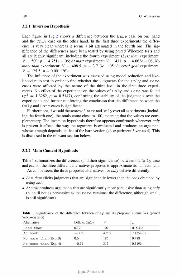
194 G. Winterstein
3.2.1 Inversion Hypothesis
Each figure in Fig. 2 shows a difference between the Bare case on one handand the Only case on the other hand. In the first three experiments the differ-ence is very clear whereas it seems a bit attenuated in the fourth one. The sig-nificance of the differences have been tested by using paired Wilcoxon tests andall are highly significant, including the fourth experiment (Less than experiment:V = 509, p = 4.751e − 06; At most experiment: V = 431, p = 4.062e − 06; Nomore than experiment: V = 408.5, p = 3.713e − 05: Inverted goal experiment:V = 125.5, p = 0.001126).
The influence of the experiment was assessed using model reduction and like-lihood ratio test in order to find whether the judgments for the Only and Barecases were affected by the nature of the third level in the first three experi-ments. No effect of the experiment on the values of Only and Bare was found(χ2 = 1.3282, p = 0.5147), confirming the stability of the judgments over theexperiments and further reinforcing the conclusion that the difference between theOnly and Bare cases is significant.
Furthermore, ifwe add the scores ofBare andOnly over all experiments (includ-ing the fourth one), the totals come close to 100, meaning that the values are com-plementary. The inversion hypothesis therefore appears confirmed: whenever onlyis present it affects the way the argument is evaluated and produces an argumentwhose strength depends on that of the bare version (cf. experiment 3 versus 4). Thisis discussed in the relevant section below.
3.2.2 Main Content Hypothesis
Table1 summarizes the differences (and their significance) between the Only caseand each of the three different alternatives proposed to approximate its main content.
As can be seen, the three proposed alternatives for only behave differently:
• Less than elicits judgments that are significantly lower than the ones obtained byusing only.
• At most produces arguments that are significantly more persuasive than using only(but still not as persuasive as the Bare versions: the difference, although small,is still significant).
Table 1 Significance of the difference between Only and its proposed alternatives (pairedWilcoxon tests)
Alternative Diff. w. Only V p
Less than 6.79 107 0.00336
At most −14.2 425.5 7.435e-05
No more than (Exp. 3) 0.6 185 0.488
No more than (Exp. 4) −0.71 317 0.5193
Layered Meanings and Bayesian Argumentation: The Case of Exclusives 195
• No more than is not significantly different from only in experiment 3. This iswhat prompted the choice of this version for experiment 4 where no significantdifference arises either. This supports the idea that No more than is an appropriateway to paraphrase the argumentative component of only.
Therefore, from the argumentative point of view and in the cases at hand, the bestparaphrase for only is given by using the expression no more than.
3.3 Discussion
3.3.1 Inversion Hypothesis
The results of the experiments confirm the inversion hypothesis: the use of onlydrastically affects the argumentative orientation of its host argument in the cases athand. I showed it to be true in the specific case where the quantity of positive andnegative evidence that should be understood by the subjects is equivalent. Thereforethe prediction that I attributed to the Bayesian reasoning approach on the grounds ofits treatment of the argument of ignorance is falsified.
It is important to note here that the inversion hypothesis does not necessarily pre-dict that the results of experiment 4 should mirror those of the first three experimentsfor the levels Bare and Only. The hypothesis merely predicts that the use of onlyshould affect the evaluation of the argument in a direction that is opposite to the onedefended by the Bare version. It does not however entail anything on the strengthof the produced argument. In other words, the fact that the gap between these twolevels is less important in experiment 4 than in the others does not argue against theinversion hypothesis.
A related issue is that if we compare the values for Only between the exper-iments 3 and 4, the difference is not significant (Wilcoxon non-paired test, W =15758.5, p = 0.6817). Furthermore, both scores lie around the middle of the possi-ble range of values (48.2 for the first experiment, 46.7 for the inverted experiment).
Seeing that the value for only does not seem affected by the shift in argumentativetarget and that the scores for the Only sentences lie around the middle of the rangeof possible values, one could hypothesize that subjects have a hard time interpretingexamples involving Only and that instead of properly evaluating the argumentsthey always choose a middle range value as a kind of default. The choice for thisdefault could be motivated on the grounds that the sentences involving only are morecomplex to treat and thus that subjects who are unsure might resort to a kind ofnon-committal “safe haven”.
I have no decisive argument to turn down this interpretation but I believe it isnot right on track. My intuition is based on the fact that in the inverted goal experi-ment, evaluating the Only case should be more easy than evaluating the Bare casesince the conclusion that is explicitly given is supported by Only while Bare goesagainst it. So even though the sentence is more complex, its argumentative evaluation

196 G. Winterstein
should be facilitated. This could also be a way to explain how the strength of theargument is affected when using a reversal operator like only, which could be a wayto account for the fact that the gap in experiment 4 is less important that in the otherthree. More work should however be done on the cost of processing an utteranceagainst an explicit conclusion for this last argument to be valid.
3.3.2 Main Content Hypothesis
Regarding the main content hypothesis, we saw that no more than is the formulationthat matches the argumentative behavior of only. Therefore we can accept the maincontent hypothesis if we assume that no more than aptly represents the main contentconveyed by only. Since this has been assumed before and appears relevant for thestudied examples, the conclusion seems reasonable enough. However it should bekept in mind that this paraphrase is not always appropriate. First of all, it essentiallyapplies when the associate of only is scalar. In a non-scalar case like (20) replacingonly by no more than does not appear very natural, at least not as an answer to “Whocame to the party?”
(20) a. Only Lemmy came to the party.b. ? No more than Lemmy came to the party.
Furthermore, as pointed out in (Winterstein 2012), in some cases only does notyield an inversion effect but rather appears to strengthen an argument. This is intu-itively the case in (21-a) which argues for (21-b) both with and without only. It isargued that this happens when the associate of only occupies the top of a scale.
(21) a. Lemmy only drinks single malt scotch.b. �
argLemmy is a connoisseur of whisky.
In those cases replacing only by no more than would probably not be a goodargumentative paraphrase. The same could also be said for at most which is alsopurported to be a good approximation of the main content of only.
Such a case is interesting for the main content hypothesis. For (21-a), one couldparaphrase the main content as in (22).
(22) Lemmy does not drink low and middle range whiskies.
Intuitively, (22) argues in favor of (21-b), so the main content hypothesis can bemaintained even in the case of (21-a).As claimed in (Winterstein 2012), the advantageof this position is that this entails that the argumentative profile of only can be derivedfrom its semantics without having to postulate it as a primitive meaning (which isthe traditional way of treating argumentation in the linguistic perspective).

Layered Meanings and Bayesian Argumentation: The Case of Exclusives 197
3.3.3 Bayesian Reasoning
Assuming that the previous hypotheses are correct, we can draw a refined accountof the way the Bayesian interpretation of natural language takes place. Essentially,I make more precise the nature of the content that is used for the conditional updateof the speaker’s beliefs by stating that only the at-issue content is used.
Assuming, with Zeevat (2013, 2014), that looking for the interpretation I of anutteranceU means finding I such that argmaxI p(I )p(U |I ), then this last hypothesisreduces to say that in this process, U is restricted to its at-issue content in thisoperation.
The exact extension of the notion of interpretation is beyond the scope of thepaper. However, one can assume that the speaker’s goal, i.e. the proposition he orshe wishes to support by making his assertion, does belong to I . Therefore, theprocess of abduction of the argumentative goal is also constrained by themain contenthypothesis: when figuring out the potential goals the speaker might be defending,the reasoning is only done by considering the at-issue part of the argument.
We apply this hypothesis to the case of (11) (repeated here).
(11) a. Half the studies showed that drug X has undesirable side-effects.b. Only half the studies showed that drug X has undesirable side-effects.
According to the main content hypothesis, the contents considered in the updateare:
(11-a) : Half the study showed that drug X has undesirable side-effects.= E(11-b) :No more than half the study showed that drug X has undesirable side-effects.
≡ Half the study did not show that drug X has undesirable side-effects.= ¬E
Let’s define GE = {p|P(p|E) > P(p)}, i.e. the set of goals for which E isan argument and G¬E = {p|P(p|¬E) > P(p)} the corresponding set for ¬E . Asshown above, we have T ∈ GE and¬T ∈ G¬E . In the case of (11-a), determining theinterpretation of the utterance entails determining a subset of GE that will correspondto the goals attributed to the speaker. In the case at hand we can consider that thediscourse situation induces a simple bipartition, i.e.: GE ⊂ {T,¬T }, the speakerargues either in favor or against the toxicity. Since ¬T is not in GE , we then attributeT as being the goal targeted by (11-a). The same reasoning applies for (11-b).
A more complex situation would not have involved a simple bipartition. In thatcase, determining the speaker’s goalwould have impliedfinding out the element H ′ ofGE that satisfies somecriterion.Aplausible onewould be that H ′ had to be the one thatmaximally affects the probability of asserting E , i.e. H ′ = argmaxH p(H)p(H |E),which follows the intuition mentioned above regarding I.
On a final note, we can also wonder how to integrate the contribution of presuppo-sitions in the argumentative reasoning. As suggested by a reviewer, presuppositionscould be treated as constraints on the prior probability. In (11-b), this wouldmean thatthe prior P(T ) should be affected by the knowledge of E , i.e. set to P(T ′) = P(T |E),before being updated to P(T ′|¬E). The problem with this hypothesis is that it con-tradicts the main content hypothesis and predicts that both versions of (11) should

198 G. Winterstein
argue in the same way (cf. the discussion on the argument of ignorance in Sect. 2.2where I show that positive arguments “win” over negative ones).
Therefore, if presuppositions enter the picture of argumentation reasoning, theyhave to be treated in a different manner. It is rather plausible that they might affectprior probabilities in a way. The protocols presented here cannot however shed lighton the matter and I have to leave this to future work.
4 Conclusion
Using the specific case of the semantics of only I tried to bridge the gap betweenBayesian theories of reasoning and theories that deal with the interpretation of naturallanguage items. I focused on the specific case of the argumentative interpretationof natural language utterances and defended the hypothesis that natural languagearguments are evaluated on the sole basis of their at-issue content. This was backedup by various experiments.
Notably, we have seen that applying this hypothesis to the case of only makes theright predictions. An immediate consequence is that it is not necessary to postulatea specific argumentative component inherent in only. Nor did I need using any con-straint that stipulates that only’s associate has to be situated “low” on a scale. Theonly requirement we needed from only is that its main content excludes alternatives.In the case at hand the associate of only is scalar in nature which means that theonly possible alternatives must be higher on the scale than the associate itself: lowervalues do not count as viable alternatives since they are entailed by the associate. Inmy account this is not due to only but a consequence of the nature of the associateand is thus compatible with all the accounts that have such a description of the maincontent of only.
An alternative view on the facts presented in this work is to consider the wayan addressee would reason when faced with a sentence like (11-b). Since the infor-mational content is the same as (11-a) and since the speaker chose to utter a morecomplex version involving only, the addressee is entitled to infer that the speaker hasa non-standard attitude towards the contents he or she expresses and that this attitudeis expressed via only. At this point we can either assume that the meaning postulatebehind only encodes the necessary “negative” component, or we can assume that theaddressee evaluates the speaker’s specific attitude by focusing on the at-issue contentof the utterance. This corresponds to the main content hypothesis I have defendedso far, but puts it in a dialogical perspective where instead of mechanically updatingthe belief function of the agents, the process takes into account the agents attitudestowards the contents they express. Developing this account for only is left for futurework. My main point here was to underline the specific profile of only and the factthat it could be derived by focusing on its at-issue content.A more general program

Layered Meanings and Bayesian Argumentation: The Case of Exclusives 199
for research would be to evaluate in which measure one can further motivate variouslayers of meaning (presupposition, implicature etc.) as means of conveying informa-tion while keeping it hidden from some parts of the process of interpretation such asargumentation. This is left for future research.
References
Anscombre, J. C., & Ducrot, O. (1983). L’argumentation dans la langue. Liège, Bruxelles: PierreMardaga.
Atlas, J. D. (1993). The importance of being only. Journal of Semantics, 10, 301–318.Beaver, D. I., & Clark, B. Z. (2008). Sense and sensitivity: How focus determines meaning. Oxford:Wiley-Blackwell.
Besnard, P., & Hunter, A. (2008). Elements of argumentation. Cambridge: MIT Press.Beyssade, C. (2010). Seulement et ses usages scalaires. Langue Française, 165(1), 103–124.Coppock, E., & Beaver, D. (2013). Principles of the exclusive muddle. Journal of Semantics. doi:10.1093/jos/fft007.
Ducrot, O. (1973). La preuve et le dire. Paris: Mame.Geurts, B., & van der Sandt, R. (2004). Interpreting focus. Theoretical Linguistics, 30, 1–44.Hahn, U., & Oaksford, M. (2006). A Bayesian approach to informal argument fallacies. Synthese,
152, 207–236.Hahn, U., & Oaksford, M. (2007). The rationality of informal argumentation: a Bayesian approachto reasoning fallacies. Psychological Review, 114(3), 704–732.
Hamblin, C. L. (1970). Fallacies. London: Methuen.Horn, L. (1969). A presuppositional analysis of only and even. In: R.I. Binnick et al., (Eds.) Papers
from the Fifth Regional Meeting (pp. 318–327). Chicago Linguistic Society.Horn, L. (2002). Assertoric Inertia and NPI Licensing. In The Panels, CLS (Vol. 38, pp. 55–82).Chicago Linguistics Society.
Ippolito, M. (2008). On the meaning of only. Journal of Semantics, 25(1), 45–91.Jayez, J. (2010). Projective meaning and attachment. In M. Aloni, H. Bastiaanse, T. de Jager, &K. Schulz (Eds.), Logic, language and meaning (pp. 325–334). Berlin: Springer.
Jayez, J., & Tovena, L. (2008) Presque and almost: How argumentation derives from comparativemeaning. In O. Bonami, P. C. Hofherr (Eds.) Empirical issues in syntax and semantics, (Vol. 7,pp. 1–23). CNRS.
Krifka, M.: Additive particles under stress, In Proceedings of SALT 8 (pp. 111–128). CLC Publi-cations, Cornell (1999).
Merin, A. (1999). Information, relevance and social decision-making. In L. Moss, J. Ginzburg, &M. de Rijke (Eds.), Logic, language, and computation (Vol. 2, pp. 179–221). Stanford: CSLIPublications.
Oaksford, M., & Chater, N. (2007). Bayesian rationality—the probabilistic approach to humanreasoning. Oxford: Oxford University Press.
Oaksford, M., & Hahn, U. (2004). A Bayesian approach to the argument from ignorance. CanadianJournal of Experimental Psychology, 58, 75–85.
Pearl, J. (2009). Causality: Models reasoning and inference (2nd ed.). New York: CambridgeUniversity Press.
van Rooij, R., & Schulz, K. (2004). Exhaustive interpretation of complex sentences. Journal ofLogic, Language and Information, 13, 491–519.
Rooth, M. (1992). A theory of focus interpretation. Natural Language Semantics, 1, 75–116.Simons,M., Tonhauser, J., Beaver, D., &Roberts, C. (2010).What projects andwhy. InProceedings
of Semantics and Linguistic Theory (SALT) 20 (pp. 309–327). CLC Publications.Walton,D.N. (1996).Arguments from ignorance. Philadelphia: Pennsylvania StateUniversity Press.

200 G. Winterstein
Winterstein, G. (2012). ‘Only’ without its scales. Sprache und Datenverarbeitung, 35–36, 29–47.Zeevat, H. (2009). Only as a mirative particle. Sprache und Datenverarbeitung, 33, 179–196.Zeevat, H. (2013). Accommodation in communication. Manuscript. ILLC: University ofAmsterdam.
Zeevat, H. (2014). Language production and interpretation: Linguistics meets cognition. Leiden:Brill.
Zenker, F. (Ed.). (2013). Bayesian argumentation: The practical side of probability. Dordrecht:Springer.
Variations on a Bayesian Theme: ComparingBayesian Models of Referential Reasoning
Ciyang Qing and Michael Franke
Abstract Recent developments in Bayesian experimental pragmatics have receivedmuch attention. The Rational Speech Act (RSA) model formalizes core concepts oftraditional pragmatic theories quantitatively and makes predictions that fit empiricaldata nicely. In this paper, we analyze the RSAmodel and its relation to closely relatedgame theoretic approaches, by spelling out its belief, goal and action components.We introduce some alternatives motivated from the game theoretic tradition andcompare models incorporating these alternatives systematically to the original RSAmodel, using Bayesian model comparison, in terms of their ability to predict relevantempirical data. The result suggests that theRSAmodel could be adapted and extendedto improve its predictive power, in particular by taking speaker preferences intoaccount.
Keywords Referential expressions · Scalar implicature · Pragmatic reasoning ·Referential game · Bayesian pragmatics · Rational speech-act theory · Game-theoretic pragmatics · Experimental pragmatics · Bayesian analysis · Model com-parison
1 Introduction
Human language communication is efficient, in that people need not always sayevery detail in order to be understood. Rather, speakers often only say what is mostrelevant, and listeners can often seemingly effortlessly grasp the intended meaningbeyond what is literally said. This ability to do pragmatic inference has been long
C. Qing (B)Linguistics, Stanford University,Stanford, CA, USAe-mail: [email protected]
M. FrankeLinguistics, University of Tubingen,Tubingen, Germany
© Springer International Publishing Switzerland 2015H. Zeevat and H.-C. Schmitz (eds.), Bayesian Natural Language Semanticsand Pragmatics, Language, Cognition, and Mind 2,DOI 10.1007/978-3-319-17064-0_9
201
202 C. Qing and M. Franke
studied and the conversational implicature theory by Grice (1975) is one of the mostprominent theories in the field. However, since it is hard to formalize theCooperativePrinciple and the Conversational Maxims, Grice’s theory is not precise enough togive empirically testable predictions, especially quantitative predictions.
The Bayesian Rational Speech Act (RSA) model attempts to address this issue byusing information-theoretic notions together with the Bayesian inference framework(Frank et al. 2009; Frank and Goodman 2012; Bergen et al. 2012; Goodman andStuhlmüller 2013). It has been shown that the model could yield quantitative pre-dictions that are highly correlated to actual human judgments (Frank and Goodman2012; Goodman and Stuhlmüller 2013).
Despite the RSA model’s theoretical promise and empirical success, if we ana-lyze the design of the model, we will find several choices that are not prima facieobvious and might thus need further consideration and justification. These choiceshave their alternatives in closely related game-theoretic approaches to pragmatics(Rabin 1990; Stalnaker 2005; Benz and van Rooij 2007; Franke 2011; Jäger 2013),which have similar but slightly different conceptual motivations. Hence it is impor-tant to systematically compare the original RSAmodel with all these alternatives andtest their predictions on empirical data, so as to gain a better understanding of therelation between these models. Doing so will help illuminate the theoretical com-mitments and empirical implications of each design choice, which will enhance ourunderstanding of the nature of human pragmatic inference.
The outline of the paper is as follows. Section2 introduce the referential communi-cation games investigated by Frank andGoodman (2012) and the original RSAmodelproposed there. Section3 analyzes a few design choices in this model and introducestheir alternatives in game theoretic pragmatics, emphasizing the distinction betweenbelief, goal and action and unifying various models as different interpretations ofthese three components. Section4 reports on the results of an experiment similar toFrank and Goodman (2012). In Sect. 5, we compare the predictions of different mod-els of our new data. Finally, we discuss the implications of the results of the modelcomparison in Sect. 6, concluding that the original RSA model can be improvedon, in particular by taking speaker preferences into account, but we also point outthat a more complex picture of probabilistic pragmatic reasoning about referentialexpressions awaits further exploration.
2 Referential Games and the RSA Model
Referential games are confined interactive reasoning tasks used to study pragmaticinference in a controlled environment (Stiller et al. 2011; Frank and Goodman 2012;Degen and Franke 2012). A referential game consists of a set of objects called acontext. For example, a context might contain different shapes of different colors invarious arrangements, such as shown in Fig. 1a. The speaker in the game is asked torefer to one of the objects (the target) by uttering an expression (typically a singleword denoting a feature, i.e., color or shape, of the target) to the listener. The listener,

Variations on a Bayesian Theme … 203
t1 t2 t3
t1 t2 t3“Green”: m1 1 1 0“Circle”: m2 0 1 1“Square”: m3 1 0 0
“Blue”: m4 0 0 1
(a) (b)
Fig. 1 A simple referential game, as used in Frank and Goodman (2012). a Example content: greensquare and circle, and blue circle. b Vocabulary and truth table
who does not know which object is the target, needs to recover the target based onthe speaker’s choice of expression.
Let us first try to play this game ourselves, to get a better sense of what it isabout and why it is relevant to human pragmatic reasoning. For simplicity let usassume that the utterances that the speaker is allowed to use are from a vocabularywhich is commonly known between the speaker and the listener. The content of thevocabulary and the (truth-conditional/literal) meaning of each word are shown inFig. 1b. Suppose we play as the speaker and the target is t1, the green square. We caneither use “Square” or “Green” to truthfully refer to it, but it seems more prudent touse “Square”, as there is only one square in the context and thus the listener can easilyidentify it, whereas there are two green objects, which makes “Green” ambiguous.In terms of the Gricean Maxim of Quantity, we should use “Square” because itis more informative than “Green” in the given context; the surplus informativitymoreover seems relevant. Similarly, we should use “Blue” to refer to t3, the bluecircle. However, using “Blue” to refer to the blue circle might intuitively sound alittle unnatural, as color terms are usually used as adjectives,1 while we usuallyuse nouns to refer to concrete objects. This inclination becomes more evident whenwe want to refer to t2, the green circle. While “Green” and “Circle” are equallyambiguous in this case, we might nevertheless prefer the latter.
Now let us turn to play as the listener. If we hear “Square” or “Blue”, we easilyknow the intended referent as there is no ambiguity, but what if we hear “Circle”(or “Green”)? There are two circles in the context that we need to choose from.On the one hand, the blue circle, having the unique color in the context, seems to beperceptually dominant and thus easily captures our attention. On the other hand, fromthe previous analysis we know that if the blue circle were the intended referent, thespeaker could have chosen “Blue”which is not ambiguous and thusmore informative.Hence the listener needs to balance two sources of information, i.e., the (presumablysubconscious) perceptual salience of different objects and the rational expectationof the likelihood of the speaker making the utterance for each object.
To test these intuitions, Frank and Goodman (2012) recruited 745 US participantsvia Amazon’s Mechanical Turk to take part in a one-shot referential game, eitheras the speaker or the listener. The context of the game always consisted of threeobjects (e.g., Fig. 1a). Each object had three features: color (red, blue, or green),
1They are used as nouns mostly to refer to the colors themselves.

204 C. Qing and M. Franke
(a) (b) (c)
(d) (e) (f)
(g)
Fig. 2 Sample contexts for the 7 conditions used in Frank and Goodman (2012). The targets areindicated by dotted lines. Condition n/m means that the target has one feature shared by n objectsand another feature shared by m objects in the context (including the target itself). For 2/2, eitherthere is an object identical to the target, or the features are shared by different objects. a 1/1. b 1/2.c 1/3. d 2/2: identical (two striped squares and one dotted circle). e 2/2: different. f 2/3. g 3/3
shape (circle, square, or cloud), and texture (solid, or polka-dot, or striped). Everycontext had one feature fixed for all objects and the other two features systematicallyvaried. The objects were randomly permuted and the target object was randomlyassigned. Depending on how many objects shared the same value of a feature withthe target, contexts were classified into 7 categories (see Fig. 2): 1/1, 1/2 (the target’sfirst feature is unique, and there is another object sharing the same value of the secondfeature with the target), 1/3, 2/2 with the same object sharing both features with thetarget (which means there is another object identical to the target), 2/2 with differentobjects sharing the features, 2/3 and 3/3. The speakers were asked to choose a featureto refer to the target object.2 In order to measure the perceptual salience, some of thelisteners were told that the speaker was using a language that they did not understandand then they were asked to guess the intended referent. Other listeners were tolda feature of the target and asked to choose the intended referent. Note that listenerswere presented with pictures without dotted lines surrounding the target so they didnot know the target. For each category in each of the speaker, salience and listenerconditions, there were roughly 50 responses.3
The result of the experiment showed that speakers generally followed Grice’sMaxim of Quantity, i.e., they tried to be informative by choosing themost unique fea-ture of the target,4 and that listeners were influenced by both the perceptual salience
2More accurately, participants were ask to bet on features and referents. We will discuss this designchoice when contrasting it with our replication in Sect. 4.3As we can see, despite the fairly large number of participants recruited, the data in each conditionare not that many. Also there might be a concern that some conditions might look less interestingthan others. Again we will discuss these issues when we introduce our own replication in Sect. 4.Here we note that variety is important in order to test the general validity of a pragmatic theory.Thus the design used in Frank and Goodman (2012) served its purposes well, but may be adaptedwhen the goal is different.4Speakers’ preference was not taken into account in Frank and Goodman (2012), so all featureswere randomly assigned and later lumped together in the analysis.
Variations on a Bayesian Theme … 205
and the informativeness of the utterance that the speaker produced. However, thedata, being quantitative in nature, cannot be fully explained by a classical qualitativeGricean account of scalar implicatures, so that a major challenge in terms of formalmodeling becomes how to quantify notions such as informativeness and perceptualsalience, and how these should be integrated to yield qualitative predictions.
The rational speech-act model (RSA) model addresses these issues by usinginformation-theoretic concepts to measure informativeness and Bayesian inferenceto integrate different sources of information (Frank et al. 2009; Frank and Goodman2012; Bergen et al. 2012; Goodman and Stuhlmüller 2013). In order to measure theinformativeness of an utterance, the RSA model starts with the literal listener whoupon receiving an utterance m does a conditioning on its literal meaning:
ρ0(t | m) = U(t | �m�), (1)
where U is a uniform distribution over all the possible referents. The informativenessof utterance m for the intended referent t can be measured as the negative Kullback-Leibler divergence of the induced literal listener’s belief ρ0 from the speaker’s ownbelief δt :
Info(m, t) = −KL(δt‖ρ0) = −∑
t ′δt (t
′) log(
δt (t ′)ρ0(t ′)
), (2)
where δt is a delta distribution with all probability mass on target object t , as thespeaker knows her intended referent:
δt (t′) =
{1 if t ′ = t0 otherwise
. (3)
The speaker acts sub-optimally by choosing the utterance that soft-maximizes herexpected utility, which is defined as the informativeness of the utterance subtractedby its cost:
σ(m | t) ∝ exp(λS · U(m, t)) = exp(λS · (Info(m, t) − Cost(m))), (4)
where λS is a parameter measuring the speaker’s degree of rationality, i.e., to whatextent the speaker sticks to the strict optimum.5 The cost term is used to encodepreference in different utterances, be it about the utterances’ lengths or syntacticcategories.
5Mathematically, it can be shown that when λS = 0, σ(m | t) is uniformly distributed over allmessages,meaning that the speaker just randomly selects one of themessageswithout any optimalityconsideration. On the other hand, when λS → ∞, σ(m | t) is non-zero only when m yields themaximal utility, meaning that the speaker only selects the strictly optimal option(s). This rule iswidely used in the AI literature (e.g., Sutton and Barto 1998) and is also known as exponentialchoice rule.
206 C. Qing and M. Franke
From (1)–(4) we obtain the speaker’s production rule6:
σ(m | t) ∝ exp(λS · (logU(t | �m�) − Cost(m))) . (5)
The pragmatic listener in the RSA model, upon receiving the utterance m, per-forms a Bayesian update on his prior belief S(t) by using an estimate of the speaker’sbehavior in (5):
ρ(t | m) ∝ S(t) · σ(m | t) . (6)
Bayes’ rule naturally integrates the perceptual salience of eachobject,which is treatedas the prior S(t) and can be empirically measured, with listener’s expectation of thespeaker being informative, which is incorporated as the likelihood, thus addressingthe previously mentioned challenge of balancing different sources of information.Setting λ = 1 and Cost(m) = 0 for all m, Frank and Goodman (2012) obtained ahighly significant correlation between themodel prediction and their experiment dataon actual speaker and listener behavior gathered from referential games of varyingcomplexity.
3 Alternatives in Design Choices
The RSA model has a theoretical advantage over traditional formal pragmatic theo-ries in that it provides quantitative predictions, and it has been shown to fit relevantempirical data well. However, if we want to learn more about pragmatic reason-ing about referential expressions, it will be worthwhile to examine RSA carefullyto pin down its major components, to spell out its main design choices and theirunderlying assumptions, and to test their contribution to the predictive power of themodel through statistical comparison with natural alternatives. In this section, wewill therefore compare the RSAmodel to closely related game theoretic approaches,that likewise assume that speakers and listeners form cascading beliefs about mutualbehavior and seek to optimize their behavior based on these beliefs (Rabin 1990;Stalnaker 2005; Benz and van Rooij 2007; Franke 2011; Jäger 2013).7 We willdescribe a class of potential alternatives to RSA and then compare the predictivepower of these alternatives on relevant empirical data in later sections.
6Note that we can further simplify (5) as follows: exp(λS · (logU(t | �m�) − Cost(m))) =exp(λS logU(t | �m�) · exp(−λS · Cost(m)) = (U(t | �m�))λS · exp(−λS · Cost(m)). Incidentally,if we do not take costs into account, i.e., let Cost(m) = 0, then (5) reduces to σ(m | t) ∝ (U(t |�m�))λS , which is effectively a power rule that soft-maximizes U(t | �m�). In this respect (5) canbe seen as an action-oriented speaker model (the exact definition of which will be given in thenext section) equipped with a different kind of soft-max rule. However, we note that this is a meretechnical coincidence, and as a first step, throughout this paper we only consider the exponentialrule as the soft-max rule. Worthy et al. (2008) provide a detailed discussion and empirical analyseson the differences between the exponential and power rules.7See Franke and Jäger (2014) for overview and comparison of game theoretic and Bayesian models.

Variations on a Bayesian Theme … 207
There are three closely related notions, i.e., belief, goal and action, that play acrucial role in RSA as well as game theoretic models. The relation and distinctionbetween them can be best illustrated by looking at (5), repeated here:
σ(m | t) ∝ exp(λS · (logU(t | �m�) − Cost(m))) .
The term U(t | �m�) is the speaker’s belief about the listener’s interpretation of theutterance. The expected utility U(m, t) = logU(t | �m�) − Cost(m) describes thespeaker’s goal of communication, i.e., inducing a belief that is as close as possibleto her own with minimal effort. The production rule σ(m | t) on the left-hand sidespecifies the speaker’s action, as it defines the probability with which, according toRSA, speakers would choose a particular expression. The soft-max rule connectsthese notions, as a (sub-)rational agent’s action depends on his belief and goal.While the RSA and game theoretic models all share this general architecture intheir designs, they vary in the specific interpretations of the three ingredients, whichreflect different views and emphasis on language and communication and give rise toa series of interesting and important empirical questions. Again, let us continue withthe speaker model (5) to illustrate some points of divergence and formally define thecorresponding alternatives.
First of all, although it is prima facie reasonable to hypothesize, as Frank andGoodman (2012) do, that the empirically measured perceptual salience S(·) is com-mon knowledge between speaker and listener, it does not actually affect RSA’s pro-duction rule (5) at all. This makes it unclear in what sense the speaker can be said toknow the listener’s perceptual salience, since neither his beliefs nor actions dependon it. A natural variant, which is used in some game theoretic models, would be toreplace the literal listener’s uniform distribution U(t) in (1) with the salience priorS(t). This leads to the alternative production rule:
σS(m | t) ∝ exp(λS · (logS(t | �m�) − Cost(m))) . (7)
Secondly, RSAmeasures the informativeness of an utterancem, which is a crucialpart of the communicative goal, in terms of how close the induced belief of theliteral listener is from the speaker’s own belief. This means that the RSA modelsees the goal of communication as conveying belief. While it is normally true thatlanguage does convey the belief of the speaker, it is questionable at least in thisreferential scenario whether letting the listener form a proper belief is the ultimategoal of the communication. After all, if the speaker wants to refer to something,it seems that in the end what matters is whether the listener actually picks out theintended referent successfully (e.g., when the speaker wants the listener to passsomething). This view is inherent in game theoretic approaches where agents’ beliefsare backed up by explicit formulations of their utilities. Wemight call this latter viewaction-oriented, in contrast to the belief-oriented view of communication whichthe RSA model adopts, as it interprets the goal of communication as invoking the

208 C. Qing and M. Franke
intended action rather than forming an accurate belief.8 Thus, according to thisview, the informativeness of a message would be measured as the probability ofthe listener choosing the intended referent. Formally speaking, we have the action-oriented speaker model9:
σa(m | t) ∝ exp(λS · (ρ0(t | m) − Cost(m))) . (8)
Hence we have four types of speaker models that differ in either the speaker’sbelief about the literal listener, or the speaker’s goal of communication. We nowintroduce a uniform notation σxy, x ∈ {a, b}, y ∈ {U ,S} for them:
σay(m | t) ∝ exp(λS · (y(t | m) − Cost(m))), (9)
σby(m | t) ∝ exp(λS · (log y(t | m) − Cost(m))), (10)
where U is the uniform prior and S is the salience prior. For example, in the originalRSA model, the speaker does not take listener’s salience prior into account and hehas a belief-oriented goal of communication. Thus it will be denoted as σbU .
Finally, the original RSA speaker model (Frank and Goodman 2012) hasCost(m) = 0 for allm, which means that the potential speaker preference in differentutterances is not taken into account (but not so in, e.g., Bergen et al. (2012)). As wepreviously pointed out, our intuition seems to suggest a preference for nouns overadjectives as referential expressions.10 Since it is an empirical question whether, towhat direction or to what extent such a preference exists, we leave open all the pos-sibilities. Technically speaking, since only the difference in costs matters, we definethe cost function using a constant c ∈ R
Cost(m) = c if m is an adjective and 0 otherwise . (11)
8Note that the two views are clearly intimately related, despite our emphasis on their differenceshere. An accurate belief is usually helpful for choosing a desired action. In fact, forming a belief canitself be seen as an action that the listener performs, which might well be all that the speaker caresabout in many everyday situations, e.g., casual talks or responses to inquiries of information. Also,the relevant actions might vary greatly across situations which makes belief formation a practicalalternative to serve as the goal. Nevertheless, they are still essentially different views in spite of thefact that they often coincide in practice. The referential communication scenario we investigate inthis paper reflects the distinction.9Theremight be concern aboutwhether there should be another soft-max step for the literal listener’schoice probability ρ0(t | m) in order for it to be action-oriented. This depends on the preciseconceptual status of the literal listener in the model and to our knowledge there is no consensusyet. We tend to think of a literal listener as an automatic subconscious process that involves nooptimality reasoning or decision-making. Thus we consider it appropriate to use ρ0(t | m) as theaction of the literal listener. However, we do agree that in principle there can be a model whoseliteral listener does a soft-max over the salience prior, and such a model can be similarly includedin the model comparison.10The rich tradition on referential expression generation (Kramer and van Deemter 2012) has alsoidentified the need to take speaker preferences into account, and Gatt et al. (2013) criticize RSA onthese grounds as well.

Variations on a Bayesian Theme … 209
If c > 0 it means there is a preference for nouns and if c < 0 then the preference isfor adjectives. No preference exists if c = 0.
Now we turn to the listener model (6), where the boundary between belief, goaland action becomes less clear:
ρ(t | m) ∝ S(t) · σ(m | t) .
Let us start from the relatively clear part. As pointed out previously, the likelihoodterm σ(m | t) is the listener’s belief about how the speaker behaves. One naturalquestion is to what extent the listener’s belief correlates with the actual production.We thus treat the speaker’s production term σ(m | t) in the listener’s model asa parameter, making the association with a belief about production of the listenermodel explicit:
ρ(σxy)(t | m) ∝ S(t) · σxy(m | t) . (12)
Note that the speaker’s production rule has two parameters λS, c which are alsoincluded in the above specification of the listener model.
Next, even thoughour intuition suggests different objects have different perceptualsalience and thus might affect our judgment, it is after all an empirical questionwhether it is relevant in the interpretation of referential expressions. It is in principlepossible that the listener does not take into account the perceptual salience in hisreasoning, which means he has a uniform prior over the referents:
ρU (σxy)(t | m) ∝ U(t) · σxy(m | t) . (13)
Finally, since the RSA model adopts a belief-oriented view on the goal of com-munication, its listener model only consists of the belief about the intended referentafter hearing the utterance, obtained by a Bayes update. However, according to theaction-oriented view, this is not quite the end of the story. The listener often needsto decide the exact referent of a referential expression. (Again, consider the case inwhich the listener is asked to pass something.) Hence in such cases the listener willchoose an object by, essentially, (soft-)maximizing over his beliefs. Formally, theaction-oriented listener model becomes:
ρav(σxy)(t | m) ∝ exp(λL · ρbv(σxy)(t | m)), (14)
where v ∈ {U ,S}, λL is the parameter measuring the listener’s degree of rationality,and ρbv is the belief-oriented model that does the Bayesian update:
ρbv(σxy)(t | m) ∝ v(t) · σxy(m | t) . (15)
For instance, the original RSA listener model is a belief-oriented one with the per-ceptual salience as prior, whose belief about the speaker is σbU , hence it is denotedas ρbS(σbU ).

210 C. Qing and M. Franke
Fig. 3 A sample context
4 The Experiment
In the previous section we analyzed the design of the original RSA model, spelledout the relation and distinction between belief, goal and action, and proposed afamily of alternative models based on different interpretation of these notions. Thisgives rise to a series of interesting empirical questions regarding the underlyingassumptions of themodels. In order to gain insight into these questions by comparingthe predictive power of different models, we conducted the following experiment tocollect empirical data, which we will use to test the predictions of different modelsin the next section.
Participants
We recruited 1032 US participants via Amazon’s Mechanical Turk. Each participantplayed a one-shot referential game either as a speaker or as a listener and receiveda payment of 5 cents. If a participant contributed multiple trials, only the first wasincluded. All participants passed the attention check described below.
Materials and Procedure
Each participant saw a context consisting of three objects (Fig. 3 as an example) andreported on the number of objects in the context as an attention check. Participants inthe listener conditions were told to imagine someone was talking to them who usedsome utterance (depending on the specific condition tested) to refer to exactly oneof the objects in the context. Then they were asked to choose what they thought tobe the intended referent. Participants in the speaker conditions were told to imaginethey were talking to someone and they wanted to refer to one of the objects (indicatedby a small red arrow11). Then they were asked to choose between two words to referto it.
Each context had a square and a circle sharing the same color, and another circlehaving a different color. Hence each object had two features: shape (square/circle)and color (green/blue) and each context had two ambiguous (shared by two objects)features. In the listener salience condition, participants were told that the persontalking to them was using a foreign language they could not understand, and in theother two listener conditions, the utterances used were the ambiguous feature ofshape and color, respectively. In the speaker conditions, the target could be any ofthe three objects: the one with the unique color, the one with the unique shape and theone with both features shared. The two words for the participants to choose betweenwere the features of color and shape of the target object.
11Participants were told that the arrowwas only for illustration and thus the person they were talkingto could not see it.

Variations on a Bayesian Theme … 211
In order to minimize the effect of the confounding factors, we counterbalancedthe positions and colors of the objects, as well as the orders of the candidate wordsin the speaker conditions. Thus the unique color in a context could be either blue (asin Fig. 3) or green and the order of the objects could be any of the permutations.12
Design
There are four major design choices in our own experiment that differ from the orig-inal experiment in Frank and Goodman (2012). First of all, the original experimentused a betting paradigm, i.e., participants were asked to bet over a range of optionsand they were instructed that the amount of money that is bet on an option shouldreflect their confidence that the option is correct. Even though the betting paradigmhas the merit of providing us with graded reponses from each individual participant,the caveat is that it is unclear whether it measures beliefs or actions. This can leadto confusion when we are to fit the model predictions to the empirical data withoutknowing whether they are directly comparable. In addition, since the betting para-digm is more or less introspective in nature, it tends to be not very accurate. Thuswe used a forced choice design instead, which clearly measures the action, doesnot rely on introspection and, technically speaking, provides for a straightforwardlikelihood function to be used in subsequent statistical model comparison. Secondly,since we decided to investigate the influence of the speaker’s preference as well asthe listener’s perceptual salience, we focused on contexts equivalent to Fig. 1a, whichrequire reasoning that is highly reminiscent of Gricean accounts of scalar implicaturecalculation, and examined different features separately. Thirdly, we only includedthe features of color and shape, with binary values (green/blue and square/circle) fortwo reasons. On the one hand, we wanted to ensure the vocabulary to be commonknowledge, so we excluded the feature of texture. On the other hand, we excludedfeature values red and cloud as they are significantly more salient than the others,which might override the pragmatic effect. Finally, we did not use dotted lines sur-rounding an object as the way to indicate the target to the speaker, as Frank andGoodman (2012) did, because that might unduly emphasize the feature of shape andthus be a confound in the experiment. Instead we used a small arrow pointing to thetarget.
Despite these differences, the remaining aspects in our experiment were almostidentical to those of the original one, e.g., the phrasing of the instructions.
The results of the speaker and listener conditions of our experiment are shown asfollows.
4.1 Speaker Conditions
There were 432 participants in the speaker conditions, 144 in each condition. Thenumbers of participants choosing each word in each condition are shown in Table1.
12Due to the scale of our preliminary experiment we did not counterbalance the shape of the objects,i.e., a context always had one square and two circles.

212 C. Qing and M. Franke
Table 1 Speaker conditions
Target “Green” “Square” “Blue” “Circle” Total
9 135 – – 144
– – 119 25 144
63 – – 81 144
Note that when the target was the object with the unique shape (as in the first row ofthe table), the feature of shape (“Square”) should be the optimal utterance becausethe listener could uniquely identify it. Similarly when the target was the object withthe unique color (the second row), the optimal utterance would be the feature of color(“Blue” in this case). When the target was the object with both features shared, bothfeatures should be equally ambiguous because of the context’s symmetric nature.
From the data in Table1, we can see that the speakers tend to choose the opti-mal feature more often when the target has the unique shape than when it has theunique color (χ2 = 8.5, p < 0.01). Even though they seem to prefer the feature ofshape when both of the target’s features are shared, the difference is not statisticallysignificant from uniform random choice (χ2 = 2.25, p = 0.13).
4.2 Listener Conditions
There were 600 participants in the listener conditions, 240 in the salience condi-tion and 180 in each of the remaining two conditions. The numbers of participantschoosing each object in each condition are shown in Table2.
The result of the salience condition will be used as the empirical estimation ofcontextual salience. For the other two conditions, the object with both features shared(the green circle in the above table, but note that we counterbalanced colors) iswhat the Gricean pragmatic account predicts to be the target. The result in Table2shows that when the message is “Green”, listeners prefer the green circle which ispredicted by the Gricean pragmatics, while they tend to stick to the blue circle whichis more perceptually salient when the message is “Circle”. The behavioral patternsin both conditions are significantly different from uniform random choice, and they
Table 2 Listener conditions
Total
Salience 71 30 139 240
“Green” 65 115 0 180
“Circle” 1 62 117 180

Variations on a Bayesian Theme … 213
significantly differ from each other in whether they conform to the predictions byGricean pragmatic theory.
5 Model Comparison
We use a Bayesian approach to model comparison (Jeffreys 1961; Kass and Raftery1995; Jaynes 2003; Vandekerckhove et al. in press) to find out which alternativebest explains the observed data. The models under investigation have unspecifiedparameters: the speaker’s degree of rationality λS, the cost of adjectives c, and, forthose listener models that have an action-oriented communication goal, the listener’sdegree of rationality λL. Since there is no principled theory to determine the value ofthe parameters, we will rely mostly on relatively uninformed hyperpriors (so-calledto distinguish them from the salience priors). Based on a specification of hyperpriors,we calculate the models’ evidences and compare them by their Bayes factors. Theevidence of a model M is the weighted average of the likelihood of observing thedata under all parameter values:
Ev(M) =∫
Pr(θ) · Pr(D | M, θ) dθ, (16)
where Pr(θ) is the hyperprior over parameter(-tuple) θ associated with model M andPr(D | M, θ) is the likelihood of the observed data D given M and each concreteinstantiation of the parameter(-tuple) θ. The Bayes factor K M1
M2is a comparative
measure for the plausibility of model M1 over M2, given their respective hyperpriorsand the data in question:
K M1M2
= Ev(M1)
Ev(M2). (17)
Model M1 makes the data more likely whenever K M1M2
> 1, but normally only a
Bayes factor K M1M2
> 3 (or sometimes K M1M2
> 5) is considered substantial. Values
K M1M2
> 10 are considered strong evidence.In a sense, comparison by Bayes factors is comparing models in a wider sense
of the term: we actually compare pairs consisting of a model and its associatedhyperprior. For clarity, we refer henceforth to a model-hyperprior pair as a Model.
Speaker data. First we look at the speaker models σxy, x ∈ {a, b}, y ∈ {U ,S}. Eachmodel has two parameters λS and c. We assume that they are independent of eachother:
Pr(λS, c) = Pr(λS) · Pr(c) . (18)

214 C. Qing and M. Franke
Table 3 Log-evidences of speaker models
Support ofP (c) σbU σaU σbS σaS
[0, 0] 67.48- - - --67.81 -104.14(−0.4, 0.4) -32.92 -33.15 1-81.44 -139.27- - - -
-157.75
We are uncertain about the rationality of the speaker:
Pr(λS) = U(0,11)(λS), (19)
which is a uniform distribution over (0, 11). Excluding λ-values ≥ 11 serves prac-tical purposes only, but is innocuous since the regions of non-negligible posteriorlikelihood of λ lie safely in the chosen interval for all models. Next, to allow forthe possibility of speaker preferences (nouns over adjectives or vice versa), we con-sider two types of hyperpriors for costs c. The first hyperprior has Pr(c) = δ(c), theDirac delta distribution, that assigns all probability mass to c = 0. This captures theassumption that there is no speaker preference. The second hyperprior is U(−0.4,0.4),which captures the notion that a preference exists, without commitment to eitherdirection. We restrict our attention to the interval (−0.4, 0.4), because we considerhigher levels of cost implausible, given that utilities for successful communicationlive in [0, 1] and that we believe that strive for communicative success should outrankpreference satisfaction in a rational model of communication. Taken together, thereare four speaker models, two hyperpriors for each, so that we compare eight Modelswith respect to their evidences.
Evidences of speaker Models were calculated by grid approximation. The resultsare shownas log-evidences inTable3. (Notice that theBayes factor betweenmodels iseasily comparedby taking the differences between log-evidences.)Wecan see that thedata very strongly supports speaker models that do not take the listener’s perceptualsalience into account. Also, it seems that action-oriented models are slightly betterthan their belief-oriented counterparts, even though the relevant Bayes factors arenot substantial by common standards. Finally, our data makes each speaker Modelthat does allow for a speaker preference strongly more plausible than its counterpartthat does not. A look at the posterior likelihood of c for each speaker model informsus that our data supports the belief in a speaker preference for nouns, see Fig. 4.13
In sum, our data supports the view that the speaker does not take into account theperceptual salience of the listener, while having her own preference for shape termsover color terms.
13A technical aside: formally, action-based speaker models, as formulated in Sect. 3, assign a non-zero probability to the event that a speaker chooses a descriptionwhich is not true of the target object(unlike belief-based models). But since subjects in our experiments could only select between truealternatives, the predictions of action-based speaker models were restricted to truthful choices inthe reported model comparison.

Variations on a Bayesian Theme … 215
Fig. 4 Posteriordistributions over costs giventhe data for each speakermodel
0 0.1 0.2 0.3 0.4
0
10
20
30
c
P(c
|D,M
)
σaUσbUσaSσbS
Listener data. Each listener model has a speaker model nested inside as a belief ofthe listener about the speaker’s behavior. Section3 introduced a total of 16 poten-tially relevant listener models, but we will focus on a selection only. For one, werestrict our attention to those listener models that are either entirely belief-based orentirely action-based. In other words, we exclude as notionally inconsistent modelslike ρa·(σb·) where the receiver part assumes an action-based goal structure and thespeaker part a belief-based goal structure. For another, we assume that the listener’smodel of the speaker is a reasonable one and therefore put to the side listener modelsthat embed speaker models that are highly implausible, given the speaker data as dis-cussed above. Effectively, this discards listener models that include speaker modelsthat take the listener’s salience prior into account. These two principled restrictionsleave us with four listener models to compare.14
Further variation comes from different relevant hyperpriors. Belief-based modelsof the listener have the same parameters as speaker models: the speaker’s rationalityλS and the speaker’s preference costs c. Importantly though, hyperpriors over λSand c, although formally parallel to those for speaker models, have a different inter-pretation in listener models where they capture our prior beliefs about the listeners’beliefs about the speakers’ likely rationality and preferences. This is true as well foraction-based models, which also have an additional parameter λL. Hyperpriors forthe latter encode our prior beliefs about the listener’s actual rationality.
We consider a variety of hyperpriors that differ in whether they take the speaker’scosts into account, whether the listener’s beliefs about the speaker’s rationalityand preferences are uninformed (i.e., flat) or informed (i.e., given by the poste-rior likelihood of parameters given the actual speaker data) and, in action-basedmodels, whether the listener’s level of rationality corresponds to his “informed”beliefs. The latter option effectively implements the assumption that there is a tight
14Similar to the remarks about speaker models in Footnote 13, we need to be mindful about the factthat action-based listener models assign non-zero probability to the choice of referents of whichthe given description is not true. Here, despite the fact that subjects in our experiments could inprinciple choose referents of which the given description is not true (this indeed happened once),we restricted the predictions of these models to only semantically compatible referent choices. Wethen discarded the one data point in which a subject choose a semantically non-compatible referent.

216 C. Qing and M. Franke
correlation between the speaker’s actual rationality, the listener’s actual rationalityand the listener’s beliefs about the speaker’s rationality.
Concretely, we consider the following “flat” hyperpriors:
Pr(λS, c) = U(0,11)(λS) · Pr(c)Pr(λS, c,λL) = U(0,11)(λS) · Pr(c) · U(0,11)(λL),
for belief-based and action-based models respectively, where Pr(c) is the hyperpriorfor the speaker’s preference parameter c. When Pr(c) = δ(c) we have a hyperpriorthat does not take costs into account; otherwise we assume Pr(c) = U(−0.4,0.4)(c),as before.
Hyperpriors that capture the idea that the listener’s beliefs are good guesses ofspeaker behavior are modeled as if informed by the data from the speaker experi-ments:
Pr(λS, c) = Pr(λS, c | DS, MS)
Pr(λS, c,λL) = Pr(λS, c | DS, MS) · U(0,11)(λL) .
Here, DS is the data from the speaker experiments, and MS the relevant speakermodel. For a given listener model, we consider only the embedded speaker model asrelevant. We call hyperpriors of the above form “informed” or, in the case of action-based models, “informed uncorrelated”. We distinguish the latter from “informedcorrelated” hyperpriors of the form:
Pr(λS, c,λL) = Pr(λS, c | DS, MS) · Pr(λL | DS, MS),
where the listener’s rationality parameter is distributed according to the relevantposterior. All of the three types of informed hyperpriors were tested in two varieties:whether the listener takes the sender’s preferences into account or not. If he does not,the posterior Pr(λS, c | DS, MS) is derived from a speaker-hyperprior Pr(c) = δ(c);otherwise from Pr(c) = U(−0.4,0.4)(c).
Taken together, we consider two belief-based models, paired with four hyperpri-ors, and two action-based models, paired with six hyperpriors (see Table4). Com-paring these ten Models is meant to address the following general questions:
1. Is the goal structure assumed by participants in our task belief-based or action-based?
2. Does the listener take the estimated salience prior into account or not?3. Is the listener’s belief about the speaker’s level of rationality “correct”, i.e., in
line with the observed speaker data?4. Is the listener’s level of rationality related to the speaker’s actual level of ratio-
nality?
Answers to these questions can be found by comparing the evidences of theModels listed in Table4.

Variations on a Bayesian Theme … 217
Table 4 Log-evidences for listener models
prior type CostsρbU (σbU ) ρbS(σbU ) ρaU (σaU ) ρaS(σaU )
Flat No -24.83 -11.66 -24.06 -10.62Flat Yes -24.80 -9.84 -23.84 -10.81
Informed No -59.87 -10.44 -25.42 -8.48Informed Yes -68.43 -13.35 -24.21 -11.85
Informed-correlated No NA NA -64.70 -6.80Informed-correlated Yes NA NA -82.36 -29.01
- - - --
--
--
-
--
--
-
--
-
--
The most striking contrast is that Models that do not take the salience prior intoaccount fare much worse than those that do. The data makes a total rejection ofModels that rely on uninformative salience priors strongly plausible.
Another eye-catching feature is that there is a clear winner in the list. The singlebest Model, which is substantially better than all the others, is action-oriented andtakes perceptual salience into account. It has an informed-correlated hyperprior andassumes that the listener does not take the speaker’s preferences into account. Thisresult is highly thought-provoking, but should be takenwith a grain of salt. It might bethat wemerely got lucky by restricting the range of λS and λL just to a small region ofreasonably high posterior likelihood for these parameters. Further experimentationshould tell uswhether informed-correlated hyperpriors are goodpredictors in general.
Most generally reliable are the results fromflat hyperpriors.Here it is interesting tonote that all of the models that take salience priors into account, with the exception ofρbU (σbS) are equally plausible, by common standards of Bayes factor comparisons.This is despite the fact that action-based models have an additional parameter.
Action-based models are also better at accommodating the idea that the listener’sestimate of the speaker behavior is roughly correct. The belief-based models aresubstantially or strongly less plausible in this case. In other words, action-basedmodels, possibly due to the added flexibility of another parameter, are better atexplaining production and comprehension data in unison.
This latter point is of interest with respect to the findings of Frank and Goodman(2012) that a single parameter choice λ = 1 provided a good fit for both productionand comprehension data. The RSA model ρbU (σbS) with fixed parameter λ = 1 isa very poor predictor of our data. (We focus here on comprehension, but the sameapplies to production data.) Assuming λ = 1 as the null hypothesis of a nested-model comparison, we can use the Savage-Dickey method to compute a Bayes factor(Dickey and Lientz 1970; Wagenmakers et al. 2010). Let M be the parameterizedModel with model ρbU (σbS) and a flat hyperprior, not taking costs into account.Given our data we should adjust our beliefs in parameter value λ = 1 by the Bayesfactor (computed approximately via MCMC sampling):
218 C. Qing and M. Franke
K = P(λ = 1 | DL, M)
P(λ = 1 | M)≈ 1.25e−9
8.18e−2= 1.52e−8
where DL is the listener data. That means that our data provides very strong evidencethat the null hypothesis λ = 1 is incorrect.
6 Conclusion
Our experiment and model comparison suggest the following. (1) On the conceptuallevel, it is helpful to clarify the distinction between belief, goal and action, and theBayesian framework provides us with a natural way to structure these componentsinto a formal model. By examining each component systematically, we can explicitlyspell out the underlying assumptions and formulate alternative hypotheses to betested. (2) On the empirical level, we tested the RSA model with a family of variantsmotivated from a game theoretic perspective on communication, and in particular, weinvestigated the speaker’s preference as well as the listener’s perceptual salience. Ourdata showed amore intricate picture of the roles that various factors play in pragmaticreasoning about referential expressions.We found evidence for a correlation betweenthe speaker’s and the listener’s rationality. Either side appears to have his own biases,but appears to be negligent of the other’s. Also, an action-based view might betterreflect the goal of communication, at least in the forced-choice experimental settingthat we used. Understanding the relation between the forced-choice and the bettingparadigms would be an important next step to gain more insight into the differencesbetween action- and belief-based goal structures.
The set ofmodels wewere able to compare explicitly here does clearly not exhaustthe space of plausible candidates. For example, we excluded listener models in whichthe literal listener takes the salience prior into account. As an anonymous reviewerpoints out, this may seem paradoxical because the best listener models of our com-parison do assume that the actual pragmatic listener takes salience into account, butdoes not believe that the speaker believes that he does. But actually, there is no fric-tion here at all, because the listener model that is embedded in a speaker model is adifferent one from the full pragmatic listener model. If we think of the pragmatic lis-tener as simulating his own hypothetical speaker behavior, there is nothing puzzlingabout factoring in salience only at a higher level of pragmatic inference.
A similar issue arises with respect to the rationality parameters in action-basedlistener models. We assumed that there are two rationality parameters, one for thelistener’s actual rationality and one for the listener’s beliefs about the speaker’srationality. But we also saw that a model that correlates the set of joint values of theseparameter pairs gave the best predictions of our data. This raises many interestingissues for further research, most of which we cannot answer here. The most obviousidea is, of course, to equate the speaker’s and the listener’s lambda and so that thelistener would believe that the speaker is exactly as rational as the listener himself.Surprisingly, this model achieves a very poor fit on our data, despite its parsimony.

Variations on a Bayesian Theme … 219
More research into correlations in perspective-taking and beliefs in rationality willhopefully shed more light on this fascinating issue.
In summary, our work shows that careful conceptual analysis of the design choicesfor quantitative models can lead to a better understanding of the phenomenon andfurther improvement in the formalmodel’s predictive power. Of course, our restrictedempirical data can only serve as a start and more data is needed to fuel furthermodel comparison towards a more robust pragmatic theory of people’s probabilisticreasoning about referential expressions.
Acknowledgments We are indebted to Judith Degen, Michael C. Frank, Noah D. Goodman andDaniel Lassiter, two anonymous reviewers, and the audience of the ESSLLI workshop “BayesianNatural Language Semantics and Pragmatics” for stimulating feedback and discussion.Many thanksalso to Henk Zeevat and Hans-Christian Schmitz for organizing mentioned workshop, and to WillFrager for help realizing our experiments.Michael Franke gratefully acknowledges financial supportby NWO-VENI grant 275-80-004.
References
Benz, A., & van Rooij, R. (2007). Optimal assertions, and what they implicate. A uniform gametheoretic approach. Topoi, 26(1), 63–78. doi:10.1007/s11245-006-9007-3.
Bergen, L., Goodman, N. D., & Levy, R. (2012). That’s what she (could have) said: How alternativeutterances affect language use. In N. Miyake, D. Peebles, & R. P. Cooper (Eds.), Proceedings ofthe 34th Annual Conference of the Cognitive Science Society (pp. 120–125). Austin: CognitiveScience Society.
Degen, J., & Franke, M. (2012). Optimal reasoning about referential expressions. In S. Brown-Schmidt, J. Ginzburg, & S. Larsson (Eds.), Proceedings of the 16th Workshop on the Semanticsand Pragmatics of Dialogue (SeineDial: SemDial 2012) (pp. 2–11). Paris: France.
Dickey, J.M.,&Lientz, B. P. (1970). Theweighted likelihood ratio, sharp hypotheses about chances,the order of a Markov chain. The Annals of Mathematical Statistics, 41(1), 214–226.
Frank, M. C., & Goodman, N. D. (2012). Predicting pragmatic reasoning in language games.Science, 336(6084), 998. doi:10.1126/science.1218633.
Frank, M. C., Goodman, N. D., Lai, P., & Tenenbaum, J. B. (2009). Informative communication inword production and word learning. In N. Taatgen & H. van Rijn (Eds.), Proceedings of the 31stAnnual Conference of the Cognitive Science Society (pp. 1228–1233). Austin: Cognitive ScienceSociety.
Franke, M. (2011). Quantity implicatures, exhaustive interpretation, and rational conversation.Semantics and Pragmatics, 4(1), 1–82. doi:10.3765/sp.4.1.
Franke, M., & Jäger, G. (2014). Pragmatic back-and-forth reasoning. In S. Pistoia Reda (Ed.),Semantics, pragmatics and the case of scalar implicatures (pp. 170–200). New York: PalgraveMacMillan. doi:10.1057/9781137333285.0011.
Gatt, A., van Gompel, R. P. G., van Deemter, K., & Kramer, E. (2013). Are we Bayesian referringexpressiongenerators? InM.Knauff,M.Pauen,N.Sebanz,& I.Wachsmuth (Eds.),Proceedings ofthe 35th Annual Conference of the Cognitive Science Society (pp. 1228–1233). Austin: CognitiveScience Society.
Goodman, N. D., & Stuhlmüller, A. (2013). Knowledge and implicature:Modeling language under-standing as social cognition.Topics in Cognitive Science, 5(1), 173–184. doi:10.1111/tops.12007.
Grice, H. (1975). Logic and conversation. In P. Cole & J. L. Morgan (Eds.), Syntax and semantics 3:Speech acts (pp. 41–58). New York: Academic Press.
220 C. Qing and M. Franke
Jäger, G. (2013). Rationalizable signaling. Erkenntnis, 79(4), 673–706. doi:10.1007/s10670-013-9462-3.
Jaynes, E. T. (2003). Probability theory: the logic of science. Cambridge: Cambridge UniversityPress.
Jeffreys, H. (1961). Theory of probability (3rd ed.). Oxford: Oxford University Press.Kass, R. E., & Raftery, A. E. (1995). Bayes factors. Journal of the American Statistical Association,
90(430), 773–795. doi:10.2307/2291091.Kramer, E.,& vanDeemter, K. (2012). Computational generation of referring expressions:A survey.
Computational Linguistics, 38(1), 173–218. doi:10.1162/coli_a_00088.Rabin, M. (1990). Communication between rational agents. Journal of Economic Theory, 51(1),144–170. doi:10.1016/0022-0531(90)90055-O.
Stalnaker, R. (2005). Saying and meaning, cheap talk and credibility. In A. Benz, G. Jäger, & R.van Rooij (Eds.), Game theory and pragmatics (pp. 83–100). New York: Palgrave MacMillan.
Stiller, A., Goodman,N.D.,&Frank,M.C. (2011). Ad-hoc scalar implicature in adults and children.In L. Carlson, C. Hölscher, & T. F. Shipley (Eds.), Proceedings of the 33rd Annual Conferenceof the Cognitive Science Society (pp. 2134–2139). Austin: Cognitive Science Society.
Sutton, R. S., & Barto, A. G. (1998). Reinforcement learning: An introduction. Cambridge: MITPress.
Vandekerckhove, J., Matzke, D., & Wagenmakers, E.-J. (in press). Model comparison and theprinciple of parsimony. In J. Busemeyer, J. Townsend, Z. J. Wang, & A. Eidels (Eds.), Oxfordhandbook of computational and mathematical psychology. Oxford: Oxford University Press.
Wagenmakers, E.-J., Lodewyckx, T., Kuriyal, H., & Grasman, R. (2010). Bayesian hypothesistesting for psychologists: A tutorial on the Savage-Dickey method. Cognitive Psychology, 60(3),158–189. doi:10.1016/j.cogpsych.2009.12.001.
Worthy, D. A., Maddox, W. T., & Markman, A. B. (2008). Ratio and difference comparisons ofexpected reward in decision-making tasks.Memory & Cognition, 36(8), 1460–1469. doi:10.3758/MC.36.8.1460.

Towards a Probabilistic Semanticsfor Vague Adjectives
Peter R. Sutton
Abstract A way of modelling the meanings of vague terms directly in terms of theuncertainties they give rise to is explored. These uncertainties are modelled with aprobabilistic, Bayesian version of situation semantics on which meaning is capturedas the correlations between uses of words and the types of situations those wordsare used to refer to. It is argued that doing so provides a framework from whichvagueness arises naturally. It is also claimed that such a framework is in a positionto better capture the boundarylessness of vague concepts.
Keywords Vagueness · Uncertainty · Probabilistic semantics · Adjectives ·Bayesian · Probability · Situations · Situation theory
1 Introduction
A seemingly characteristic feature of vague terms is their boundarylessness(Sainsbury 1991). However, a challenge for truth-conditional accounts of the seman-tics for vague terms is that truth-conditions create sharp boundaries. One way to tryto assuage this tension is to introduce uncertainty into semantics. For example, onecould maintain a threshold for truth, but model vagueness as uncertainty about wherethe threshold, in some context, lies (Lassiter 2011; Frazee and Beaver 2010). How-ever, arguably, uncertainty over thresholds nonetheless carves boundaries. In thispaper, I will avoid thresholds and develop a way of introducing uncertainty directlyinto semantic representations. On this approach, sentences are taken to encodeuncertainty over types of situations. This can been seen from two perspectives. Eitheras uncertainty about how the world is, given the way words are used, or as uncer-tainty about how to use words when faced with a type of situation to describe. Theinformation that words convey is understood as a reflection of the correlations there
P.R. Sutton (B)
Institute for Language and Information, Heinrich Heine University,Universitätsstraße 1, 40225 Düsseldorf, Germanye-mail: [email protected]
© Springer International Publishing Switzerland 2015H. Zeevat and H.-C. Schmitz (eds.), Bayesian Natural Language Semanticsand Pragmatics, Language, Cognition, and Mind 2,DOI 10.1007/978-3-319-17064-0_10
221
222 P.R. Sutton
are between features or properties in the world, and our uses of words to describe orrefer to objects with those properties. By adopting this view, I will suggest that wecan better capture the boundarylessness of terms, and that borderline cases, anothercharacteristic feature of vagueness, emerge directly from the semantics.
In Sects. 2–3 the uncertainty associated with vague terms will be described. InSects. 4–5, these informal ideas will be modelled using a probabilistic version ofsituation semantics. In Sect. 6, the approach will be linked to vagueness. In Sect. 7,the proposal will be compared with two related proposals in the recent literature.
2 Uncertainty
There are two ways that uses of a vague term can give rise to uncertainty. The firstconcerns the world and the second concerns the word. Say that we are told that Johnis tall, or that Mary’s car is green. Given that we are competent in English, and,given that we have no reason to expect what we have been told to be incorrect, whatwe have been told makes it reasonable to believe certain things about the world. Inthe vagueness literature, when the semantics of vague terms are analysed, some lessvague properties, concepts, or features are often cited in the analysis. For example,with respect to ‘green’, our judgements vary over the shades that things are; for ‘tall’,over the heights that things are; for ‘bald’, over how much (head) hair individualshave. On being told that John is tall, or that Mary’s car is green, we are uncertainabout what feature or property John has with respect to height, or that Mary’s carhas with respect to shade.
This uncertainty could be thought of as a series of graded beliefs. In the following,I will represent the content of these beliefs with reference to measures that may nothave any psychological reality. For example, I will talk about someone’s beliefs aboutheights measured in centimetres. However, it need not be assumed that our doxasticrepresentations of heights refer to centimetres. If I talk ofMary’s beliefs about John’sheight as distributing over heights in centimetres, this ismerely a convenient notation.It does not require that Mary can say, in centimetres, how tall John is (or might be).
It is, however, possible that using such precise values introduces an artificial levelof precision. It could be that the waywe cognitively represent the world is also vague,in which case, there should be a mapping from vague words to a mapping from avague representational level to properties in the world (such as being some heightin centimetres or being some particular shade). However, by describing mappingsbetween vague words and less or non-vague properties in the world directly, I am,at worst, oversimplifying the matter by skipping over a mental/cognitive level ofrepresentation. For at least some cases we ought to be able to describe how theinformation conveyed by words relates to the (more or less) precise properties to befound in situations in the world.
It would be unreasonable to believe that John is a specific height just on the basisof being told that he is tall, and it would be unreasonable to believe Mary’s car to be

Towards a Probabilistic Semantics for Vague Adjectives 223
a specific shade just on the basis of being told it is green. Herein lies the first kind ofuncertainty:
(U1) Descriptions using vague expressions leave us uncertain about specific fea-tures/properties that objects in the world have.
U1 uncertainty is often, to some extent, eliminable in practice. We can, for exam-ple, go and look at John (maybe even measure him), or we can go and have a lookat Mary’s car. And yet, even if we are in command of these facts, uncertainty abouthow to use our language can still remain. If John is 180cm tall, or if Mary’s car isan odd sort of turquoise shade, we might feel thoroughly uncertain whether or not‘tall’ would be an effective word to use to describe John or ‘green’ an effective wordto use to describe Mary’s car.
By using the term ‘effective’, I mean to appeal to a notion of success. What iseffective (for some purpose) is what succeeds in doing something/bringing aboutthe desired result. What is effective for describing John, or Mary’s car is going tobe an interest relative matter, since what is effective for doing something in onesituation may not be effective in another. A lot of the vagueness literature, insofar asit predominantly concerns solutions to the sorites paradox, takes the only importantcriterion for what is effective to be what description would be true. However, truth isnot always what we need to establish, or are interested in. For example, if our aim isto communicate which individual John is in a crowd, irrespective of whatever storyabout the truth-conditions for ‘tall’ are, one might be able to use ‘tall’ to identifyJohn because he is significantly taller than those around him. Here, what makes adescription count as true will not be addressed in detail. Instead, I will continue to usethe broader notion of effective descriptions which can be used to describe a secondkind of uncertainty:
(U2) Specific features/properties that objects in theworld have can leaveus uncertainabout how to effectively describe them.
Relations hold between U1 and U2:
1. Were we equally certain of applying ‘tall’ to 185cm John as to 190cm Bill, then,all else being equal, we should be equally certain that John (Bill) is 185cm inheight when described as tall as 190cm, and vice versa
2. Given 1, where U1 similarities give rise to U2 similarities and vice versa, weshould expect U1 differences to give rise to U2 differences and vice versa.
3. Variations in U1 uncertainty can give rise to U2 uncertainty. Being told that Johnis tall may leave us uncertain about his height. We might be fairly certain that heis not around 170cm, comparatively certain that he is around 190cm, but highlyuncertain aboutwhether he is around 180cm.Given 1 and 2, this createsU2 uncer-tainty in the use of ‘tall’. If we are fairly certain that ‘tall’ effectively describessomeone who is around 190cm in height, but fairly certain that ‘tall’ wouldn’teffectively describe someone around 170cm in height, then we should uncertainthat ‘tall’ would effectively describe someone around 180cm. Furthermore, weshould also expect a range of U2 judgements to give rise to U1 uncertainty.
224 P.R. Sutton
As emphasised by an anonymous reviewer, the presence of U1 uncertainty is notsufficient for vagueness, and the presence of U2 uncertainty is not necessary forvagueness. The relationship between vagueness and different kinds of uncertaintywill be made clear in Sect. 6. In brief, however, there will be times when, given theway the uses of words correlate with types of situations, nothing in the meaningsof the words themselves, or any outside information, will be able to resolve ouruncertainty. For example, for some heights of people, we may have irresolvableuncertainty about whether to call them tall. This can arise because when someone isdescribed as tall, we may be no more certain that they are that height than we wouldbe were they to be described as not tall.
Two challenges arise for communicating with vague expressions. As a hearer,we must face uncertainty over what objects in the world are like, given the waythey have been described. As speakers, we may, from time to time, face uncertaintyover how to effectively describe things as being. However, arguably this uncertaintystems directly from the uses of such terms, and from how such uses correlate withthe properties of situations those words describe or refer to. In the following, I willtreat the strengths of these correlations as the information that those terms carry.1
This information will be modelled using Bayesian conditional probabilities. It is inthis sense that Bayesian notions will be at the heart of the semantics for vague terms.
3 Constituents
A semantics based on uncertainty will have to be able to attribute, to types of expres-sions, a role in the larger constructions inwhich they occur. Take our above examples:‘John is tall’ and ‘Mary’s car is green’. Giving a semantics for the modifiers ‘tall’and ‘green’ can then be taken to be a matter of accounting for what information theycarry about some object. For example, ‘x is green’ might be modelled as making itreasonable to believe that x is one of some rough range of shades.
However, here a disparity between ‘tall’ and ‘green’ arises. The x in ‘x is tall’ isvital for getting any idea about what it is reasonable to believe. If we are only toldthat something, anything, is tall, be it a mountain, a molehill, a mouse, or a millipede,there is no height it would be more reasonable to believe this thing is than others.2
This changes as soon as ‘tall’ is predicated of an NP or is applied to a CN in an NP:The ‘tall’ in ‘x is a tall man’ seems to make it more reasonable to believe that x issome heights rather than others. But this suggests that part of the information whichcontributes to our expectations of heights is coming from the CN/predicate ‘man’.This can be seen by substitution of CNs/predicates.3 Compare how expectations of
1This notion of semantic information is more rigorously developed in Sutton (2013).2This may be to strong. There could be some priors we have, or reasoning we could engage in,that would make some heights more reasonable than others. My thanks go to Noah Goodman forhelpful discussion.3I do not mean to take, as assumed, a clear, semantically important division between CNs andadjectives. Below, I will treat words like ‘tall’ and ‘green’ as predicate modifiers and words like

Towards a Probabilistic Semantics for Vague Adjectives 225
heights differ for ‘x is a tall man’, ‘x is a tall molehill’ and ‘x is a tall mountain’.The situation for green seems to be similar. CNs make a difference to expectations.4
However, ‘x is green’ does seem to carry some expectations of its own: that x isroughly within some range of shades.
I take this to be a reason to see some differences in the semantics of various vagueadjectives/modifiers. The modifier ‘green’, which seems to carry information on itsown, will have a slightly different semantic shape to those modifiers (such as ‘tall’)that only seem to modify expectations based on information carried by nominalpredicates. The details of this difference will be elaborated in Sect. 5.
What we have here is an argument for treating some modifiers as, in some sense,not really carrying information per se. Instead we can see them as encoding a modifi-cation on the information carried by a nominal predicate. Someone’s being describedas a woman gives us a rough expectation as to her height. This may be a very broadrange, but we have some expectations nonetheless. Something’s being described asa skyscraper gives us very different expectations as to its height.
One might worry that this puts a lot of weight on information carried by nominalpredicates and/or background information and beliefs. However, all that is beingassumed is that learning to categorise and classify objects with such predicates, inpart, amounts to developing expectations as to basic visual cues such as size, shapeand shade. An anonymous reviewer rightly points out that this approach begins toblur the boundaries between what counts as meaning and what counts as generalknowledge about the world. A firmer distinction can be established again withoutoverly affecting the account, however. Rather that seeing the meaning of, say, ‘man’as being all the information one has learnt about men, we can view meanings as pro-cedures (see Gargett et al. 2009) for accessing such knowledge and for determiningthe ways such knowledge should be combined.
The common modifiers ‘old’, ‘big’ and ‘long’, just like ‘tall’, only seem to giveus reasonable expectations when applied to a nominal predicate (or when themselvespredicated of an NP in cases such as ‘John is tall’). In turn, however, that suggeststhat nominal predicates such as ‘man’ carry information about what features men canreasonably be expected to have. Some tests (albeit ones based on linguistic intuitions)can be applied to get a grasp on what information this is. For example, at least fornon-metaphorical uses, ‘x is a long man’ does not seem to make much sense/provideus with reasonable expectations about x’s length.5 This suggests that ‘man’ doesnot carry information pertaining to length. This is not to say that modifiers such as
(Footnote 3 continued)‘car’ and ‘man’ as predicates. In many cases, the traditional classifications of words as CNs andadjectives will overlap with these semantic divisions. Nothing I say rests on whether they all do.4This point is related to the commonly held idea that vague adjectives are context-sensitive orinterpretable only relative to a comparison class (Cresswell 1974).5In English at least, length is not simply a euphemism for height. Trains, passageways, halls, toname a few, can have a great length without having a great height.

226 P.R. Sutton
‘green’ are not restricted either. For example, synaesthesia aside, ‘x has green ideas’is hard to understand if ‘green’ relates to shade.6
Nominal predicates will be treated as encoding information based on correlationsbetween things that those common nouns are used to classify and the features thatthe things they are used to classify have. For example, it is because there is a strongercorrelation between men and some heights than there is with others, that ‘man’carries information about heights. Adjectives will be modelled as modulating somespecific aspect of the information that nominal predicates carry. For example, ‘tall’will modify information relating to height carried by predicates like ‘man’.
A possible worry can be flagged here.7 In the literature on adjectives, it is com-mon to appeal to a comparison class to capture their semantics (Cresswell 1974;Kamp 1975; Kennedy 1997; Graff Fara 2000). However, it has been pointed out thatcommon nouns do not always determine comparison classes (Kennedy 2007). Forexample, BMWs are not the comparison class below, despite featuring as part of amodified NP:
1. Kyle’s car is an expensive BMW, though it’s not expensive for a BMW. In factit’s the least expensive model they make. (Kennedy 2007)
The worry concerns whether the above analysis conflates modified nouns with com-parison classes. The analysis can, however be modified slightly. Rather than demandof some adjectives that they simply modify a nominal predicate, we can insteadrequire that there is some class of things to which it is being applied in any context(information about which can be modified by the adjective). This still leaves a differ-ence with terms like ‘red’ which seem to carry some information (about, say, shades)independently of a lexically provided nominal predicate or a comparison class.8
4 Semantics: Preliminaries
4.1 Correlations and Situations
In the following, I will suggest one way to formalise U1 uncertainty (uncertaintyover how the world is, given a description of it). I will borrow heavily fromsituation semantics (Barwise and Perry 1983; Cooper 1996; Devlin 2006), but willincorporate a probabilistic element into the standard categorical theory.
6An interesting possibility is that the application of domain specific modifiers to NPs that do notcarry information about that domain will generate metaphorical interpretations. Metaphor, humourand other such subjects are outside of the scope of this paper. There may also be an interesting linkto be explored between the ideas put forward here and work done on scalar adjectives in de Marneeet al. (2010).7This was pointed out by an anonymous reviewer for the BNLSP 2013 Workshop.8That is not to say that ‘red’ cannot relate to non-stereotypical shades (such as in ‘red onion’).Elsewhere (Sutton 2013), I suggest a way for this account to model the information carried by ‘petfish’ where goldfish are not the most stereotypical fish, nor the most stereotypical pets.

Towards a Probabilistic Semantics for Vague Adjectives 227
In situation theory, meaning is captured via the notion of constraints. Constraintsrepresent information channels, for example, types of situations in which there is rainin the city are informationally connected to types of situation in which the pavementsare wet. The (context independent) linguistic meaning of an expression is held to bejust a special case of a normal information channel: types of situation in which someexpression is uttered are informationally related to types of situations in which someconditions obtain. For example, types of situations in which someone utters ‘It’sraining in London’ are informationally connected to types of situations in whichthere is rain in (at least part of) London (at some time).
It is via this type-type link or relation that agents are able to extract token-tokeninformation. For the case in hand, if one is in a token discourse situation of the type‘It’s raining in London’ is uttered, one will be led to expect a token situation of thetype raining in London. In standard situation semantics, ignoring a lot of details, thetruth of what is said turns onwhether the token described situation is of the right type.
The basic idea to be presented in this paper is that meaning can be treated ascorrelational. Instead of constraints holding between one utterance situation type andone described situation type, probability theory will be employed to capture differentstrengths of connections between an utterance situation type, and many describedsituation types. The meanings of expressions are therefore held to be correlationsbetween discourse situations of a certain type, and described situations of a certaintype. For example, the type of situation in which ‘John is tall’ is uttered will becorrelated, to different extents, with types of situation in which John is one of manypossible heights.
In Situation Theory, situations support infons. Infons are traditionally conceivedas what contribute to forming informational items (Devlin 2006), or as types ofsituations (Cooper 1996).9 Another way to view them is as properties of situations(as opposed to properties of individuals). For example, (ignoring times) one propertythat a situation might have is where it’s raining somewhere10:
〈〈rain, l, yes〉〉
The l is a location parameter. Parameters can be seen as akin to variables. Theycan be bound via type abstraction (see below), or free. Ignoring quantifiers, freeparameters are those not bound by abstraction in situation theoretic propositions. Ifa situation, s has some property (some infon), σ, then it is said that the situation
9This way of viewing infons (as types) propagates through into situation theoretic approaches withricher type systems. See, for example Cooper (2012).10This notation for infons is essentially Devlin’s. However, for polarities, I adopt Barwise andPerry’s ‘yes’ and ‘no’ instead of Devlin’s ‘1’, ‘0’. This is to avoid potential confusion with the limitcases of probability values [0, 1].

228 P.R. Sutton
supports the infon. That a situation supports an infon, in notation, is a situationtheoretic proposition:
s � σ
For the above infon, this would give:
s � 〈〈rain, l, yes〉〉
Which says that in situation s, it is raining at some location. Situations are meant tobe ways to classify objects and events in the world. They are not possible worlds.If a situation, in fact, has the property σ (is, in fact, of type σ/supports σ), then theproposition is true.However,wewill not be seeking to associate linguistic expressionswith propositions, nor will we be directly interested in particular situations andwhether they support some infon. This is because constraints are defined betweensituation types.
Importantly, abstraction in situation theory allows one to talk about types.Abstracting over objects (understood loosely as individuals, locations, and times),creates object types. Taking our rain example, and abstracting over l, this gives:
λ[l](s � 〈〈rain, l, yes〉〉)
Which is the type of locations inwhich it rains in situations.Whenbound, parameterscan be replaced with constants as with standard β-reduction. For example:
λ[l](s � 〈〈rain, l, yes〉〉) . [London]⇒ s � 〈〈rain,London, yes〉〉
Situations can be abstracted over to give situation types11 via situation typeabstraction. Notation varies, I will adopt the following12:
λ[s](s � σ)
This means the type of situation in which σ obtains. The s is a parameter, as l above,but s is a parameter for situations. In this case, s is bound. For example:
λ[s](s � 〈〈rain,London, yes〉〉)
Which is the type of situation in which it rains in London. Correlations (informationchannels) hold between types. For example the above type might correlate with the
11More recent situation theoretic approaches take types to be objects. An example of this richtype-theoretic approach is Type Theory with Records (TTR) (Cooper 2012).12This is close to Devlin’s notation, but with Cooper’s use of ‘λ’ for abstractions instead of Devlin’s(s|s � σ). This variation is to avoid possible confusion resulting from the use of ‘|’ in probabilitytheory.

Towards a Probabilistic Semantics for Vague Adjectives 229
type of situation in which the streets of London are wet. In the probabilistic version ofSituation Theory to be developed, these correlations will be modelled as conditionalprobabilities (the probability of one type, given another). It is this that will ensurethat if some concrete situation of a type arises, there will be a probability that somesituation of another type will arise (or, arose, or will have arisen etc.).
The proposal to bemade here is then thatU1 uncertainty (where descriptions usingvague expressions leave us uncertain about specific features/properties that objectsin the world have), can be modelled as conditional probabilities between types ofsituation. I will say more on U2 probability in Sect. 7.
We will have situations of two kinds:
(i) Discourse situations, d, are situations in which some specific discourse takesplace. For example, we might have the discourse situation in which ‘red’ isused to classify some object, or, in which ‘tall’ is used to describe some person.Discourse situations will model the situations in which certain words are used(certain things are said).
(ii) Described situations, s, are situations in which the world is some way. Forexample, we might have the described situation in which an object is someshade of colour, or, in which a person is 180cm in height. Described situationswill model the kinds of ways the world can be.
Types can be formed by abstracting over discourse and described situations. Forexample:
λ[d](d � 〈〈utters, a,TALL,j, yes〉〉)
Is the type of situation in which someone describes John as ‘tall’. Given such atype, there will be a probability of some described situation being of some type. Forexample, the type of described situation in which John is 180cm in height:
λ[s](s � 〈〈height=180cm,j, yes〉〉)
Varying probabilities will result from different height values. These probabilities willform a distribution.Abstracting away from the contributionmade by the name ‘John’,this distribution will reflect the extent to which uses of the modifier ‘tall’ to describe,say, a human male, correlates with human males being certain heights. The heightsthat an agent will entertain will be restricted by her/his learning process (namely, anapproximation over the kinds of humans, males etc. that they have experienced). Itwill be supposed that a rational agent can only have distributions that sum to 1.
The information carried by sentences will be captured as the conditional proba-bility of there being a described situation of some type, given a discourse situationof some type. For example, the probability of there being a situation type in whichJohn is 5 ft, given a situation type in which John is described as tall, will be (compar-atively) very low.13 Other conditional probabilities will be greater for greater height
13This can be so even given the assumption that speakers are not being deliberately deceptive. Whatis being tracked here is the extent to which, in general, properties such as heights of individualscorrelate with types of utterances, such as describing them as tall.
230 P.R. Sutton
properties John might have. A range of such probabilities (each with a differentheight property/one-place relation assigned to John in the described situation) willform a distribution (must sum to one).
Conditional probability values will represent something like credence. However,rather than just a degree of belief, we will be concerned with the degree to which itis reasonable to believe that some state of affairs obtains. This distinction is betweenwhat, given some actual description, a hearer believes (credence), and what, in virtueof the information carried by the utterance of the words, one is entitled to believe.Conditional probability values reflect correlations between uses of words and statesof affairs. This incorporates all uses, both representations and misrepresentationsof the world. The degree to which it is reasonable that some state of affairs obtainsreflects this. Howmuch reason or entitlement one has to believe the world to be someway will be a direct reflection of how words are used (how uses of words correlatewith types of situations).
So, if being told that John is tall makes it reasonable to believe to a degree of nthat he is 180cm in height, this will be represented as assigning a probability valueof n to the conditional probability of there being a situation of the type in which Johnis 180cm in height, given a situation of the type in which he is described as tall. Thevalue for n, against another larger number, represents a lower reasonable credencein a state of affairs than the higher number. Conditional probability distributions willbe formed over a range of heights.
Types and Situation Types A more recent approach to situation theoretic seman-tics is systematically laid out in Cooper (2012) which adopts a rich proof theoretictype theory. Rather than treating types as sets of objects in a domain, this approachtreats types as objects (in a domain of types). Situations/events then act as proofs ofpropositions. In what is to follow, I will adopt a fairly simple type theory with an,essentially, model theoretic semantics.14 This simplification will make it easier tofocus on the probabilistic element in my account. A proof theoretic approach witha richer type theory could, in principle, adopt the core ideas in the proposal that Iwill make. Indeed, a probabilistic approach comparable to my own has just beenproposed in Cooper et al. (2014).15
Properties It is important to note that it is not assumed that there is anything like theproperty green or the property tall that individuals have or lack. We will be assumingthat individuals can have the property of being some height (this will just be theheight that they are). We will also be assuming that certain objects have some hue orshade.16 These heights and shade properties will be mentioned in the formalism asproperties of objects in infons.
14Thehedginghere is includedbecause, although I assumeadomainof situations (as a set), situationsare best not viewed as a set.15A difference between this, my own, and similar proposals will be explained in Sect. 7.16I assume for simplicity that these properties are not vague. Nothing turns on this however. Even ifproperties were vague in the sense that someone may genuinely be of indeterminate (exact) height,one would still need to explain how words like ‘tall’ admit of wide ranges of those properties in agraded way.

Towards a Probabilistic Semantics for Vague Adjectives 231
4.2 Definitions
Types The type system that will be used will have three basic types.17 Type e will bethe standard type for individuals (entities). Type s will be the type for situation. Ratherthan the traditional type t (for truth value), we will have type p (for probability).Basic types can be used to form functional types in the way normal to model theory.
Definition 1 Types
Basic types: {e, p, s}Functional types: If a, b are types, then 〈a, b〉 is a type
Expressions This formalism brings together notions from both probability theoryand situation theory. As such, we will need to define how various parts of theminteract. The vocabulary of the formalism is in Definition 2. Where necessary, typesof expressions will be given as subscripts. For example, a variable, S, of type 〈e, p〉will be written S〈e,p〉. The marking of numerical variables as type p in Definition 2is an oversimplification. These will be interpreted as numerical normalising values.These values can have a value outside of [0, 1], but are derivable from sums of valuesof interpretations of other type p expressions.
Definition 2 Vocabulary
Parameters (PAR): Infinite set of parameters for all types s1, . . . , d1, . . . , x, . . .
Constants (CON): A possibly empty set of constants for every typeSupports: �Conditional on: |Infons: σ, τ , 〈〈height=h,j, yes〉〉, 〈〈utters,a,TALL,j, no〉〉Connectives: ∧,¬,∨Lambda abstraction operator: λMathematical operators: ×,+,−Numerical variables: C, C′ of type 〈p〉Brackets: ( , ), [ , ]
A further few remarks on infons are needed at this juncture. Infons contain rela-tions between objects and the polarities in infons ‘yes’ and ‘no’ indicate whetherthe relation holds between the objects. I assume a basic ontology of relations (suchas being some height or being some shade). Propositions state that situations sup-port infons. Positive polarities on infons indicate that any situation that supports the
17I will from now on suppress all reference to locations and times, which are also types in situationtheory.

232 P.R. Sutton
infon is of that type. A negative polarity would indicate that the situation is of thenegative type. Infons can thus be understood as types of situations (Cooper 1996), orperhaps as properties of situations. The class of infons will be formed of all possiblecombinations of relations and objects in our ontology (plus a polarity).
The well-formed expressions of the language are defined in Definition 3 (whereWEa denotes well formed expressions of type a). Clauses (i), (ii), (iv) and (v) arestandard. Clause (v) introduces the syntax for situation types. Clause (vi) gives whatwill eventually be interpreted as a conditional probability of one situation type givenanother. The connectives in clause (vii) will be discussed in greater detail below.Clause (viii) allows for expressions of type p to be linked by mathematical connec-tives.
Definition 3 Well-Formed Expressions:
(i) If α ∈ PARa, then α ∈ WEa,(ii) If α ∈ CONa, then α ∈ WEa,(iii) If α ∈ WE〈a,b〉 and β ∈ WEa, then α(β) ∈ WEb,(iv) If α ∈ WEb, and β ∈ WEa, then λ[β](α) ∈ WE〈a,b〉,(v) If α ∈ WEs, and if σ is an infon, then λ[α](α � σ) ∈ WEp,(vi) If φ,ψ ∈ WEp, then φ | ψ ∈ WEp,(vii) If φ,ψ ∈ WEp, then:
(a) ¬φ ∈ WEp,(b) φ ∧ ψ ∈ WEp,(c) φ ∨ ψ ∈ WEp,
(viii) If φ,ψ ∈ W E p, then
(a) φ × ψ ∈ WEp,(b) φ + ψ ∈ WEp,(c) φ − ψ ∈ WEp,
As mentioned briefly earlier, there are two kinds of situation parameters thatwe will use: described situations (s) and discourse situations (d). For descriptivesituation types, we will be interested in how the world is with respect to things likethe shades things are (for colour terms), and the heights things are (for terms like‘tall’). In discourse situation types, what will be described is the production of someutterance type.
The infonswewill be concernedwith are likewise of two kinds. Infons for descrip-tive situations will describe/be about, say, what height someone is. Immediatelybelow I specify the infon, and below that, I give a described situation type includingthat infon:
〈〈height=180cm,j, yes〉〉
λ[s](s � 〈〈height=180cm,j, yes〉〉)
The latter is the type of situation in which the individual denoted by j (say, John)is 180cm in height. Infons for descriptive situation types will typically relate to

Towards a Probabilistic Semantics for Vague Adjectives 233
what has been said. For example, below, I specify a discourse infon, followed by adiscourse situation type including that infon:
〈〈utters, a,TALL,j, yes〉〉
λ[d](d � 〈〈utters, a,TALL,j, yes〉〉)
The latter is the type of situation in which the individual denoted by j (say, John) hasbeen described as tall. This is a simplification, however. In actual fact, there oughtto be unbound parameters for locations and times etc. which are being suppressedfor simplicity.
For either of these situation types (descriptive and discourse), many actual situa-tions could be of those types (types where John is 180cm in height, or where he isdescribed using ‘tall’).
Interpretations and Domains The interpretation function we shall use will bemarked as: p(·). Hence, an expression φ of type p, will be interpreted as p(φ),or the probability of φ. Like interpretation functions in model theory, the interpreta-tions of type p expressions will be built up of the interpretations of other expressions.I assume a domain for each basic type. If a is a basic type:
p(α〈a〉) ∈ Dom〈a〉
Functionally typed expressions will be interpreted as functions from basic domains:
p(α〈a,b〉) ∈ DomDom〈a〉〈b〉
The type e domain will be a set of individuals. The domain of type p will bethe range [0, 1]. Situations are being taken as primitive. We can, for the sake of theformalism, assume a domain of situations. However, in the spirit of situation theory,situations should be taken to be our ways of conceptualising and carving up the worldinto parts. As well as the interpretation function, we will have a parameter anchoringfunction g, which assigns appropriate members of the domain to parameters. Insituation theory, parameter anchoring functions have restrictions on their domains, Iwill pass over those details here.
The first four clauses of Definition 4 are fairly standard. Clause (v) simply statesthat maths operators in the object language are treated as standard when the interpre-tations of their operands are in the range [0, 1]. Clause (vi) simply states the standarddefinitions of probabilistic connectives (Kolmogorov 1950).
Spaces and Priors In order for these axioms and the probability function to bewell defined, we must define a probability space. Probabilities will distribute oversituation types. The probability value will be in the range [0, 1] where this valueindicates the probability of some situation being of the type specified by the infon.Conditional probabilities will be the probability of a situation being of some type,given that some situation is of another type. For simplicity, for all non-conditional
234 P.R. Sutton
values, I assume that probabilities distribute evenly.18 For example, in the case wherewe have n discrete ranges of heights over which a distribution will be formed, thevalues for each unconditional situation type will be:
p(λ[s](s � 〈〈height=h, x, yes〉〉)g = 1
n
Definition 4 Denotations
(i) p(x)g = g(x) if x ∈ PAR,(ii) p(c)g = p(c) if c ∈ CON ,(iii) p(α(β))g = p(α)g(p(β)g),(iv) p(λ[x](α))g = f such that if x ∈ PARa , and c ∈ Doma , f (c) = p(α)g[x :=c],(v) Maths Operators:
(a) p(φ × ψ)g = p(φ)g × p(ψ)g ,(b) p(φ + ψ)g = p(φ)g + p(ψ)g ,(c) p(φ − ψ)g = p(φ)g − p(ψ)g ,
(vi) Probabilistic Connectives:
(a) p(¬φ)g = 1 − p(φ)g ,(b) p(φ ∧ ψ)g = p(φ)g × p(ψ | φ)g ,(c) p(φ ∨ ψ)g = p(φ)g + p(ψ)g − p(φ ∧ ψ)g .
In practice, the rangeof situations and infonswill be highly constrained. For describedsituations, constraints will come out of the semantic learning process, as well asthe goals and purposes of the speakers. For example, certain ranges of shade/hueproperties will constrain the range of described situations for colour terms in general,but further constraints may come from what objects are salient to speaker and hearerin the situation of utterance.
For discourse situations, I assume a space of two infons, formed of the samerelation and object but with opposing polarities.
p(λ[d](d � 〈〈R,a1, . . .an, yes〉〉))g = 0.5 = p(λ[d](d � 〈〈R,a1, . . .an, no〉〉))g
However, when multiple terms are used, the space of possibilities may be bigger andso values may be lower.
Representationalism The formal semantics and linguistics debate over represen-tationalism got going with the publication of work on Discourse RepresentationTheory (DRT) (for an overview, see Kamp and Reyle 1993). DRT questioned Mon-tague’s claim that the representational language of a formalism is dispensable. InDRT, it was claimed that to account for the treatment of some expressions (such asdiscourse anaphora), the representational (interpretational) level is not dispensable.
18In amore sophisticatedmodel, one would wish the values of priors to be set in accordance with thelearning experiences of agents. One way this has been implemented will be discussed in Sect. 7.2.
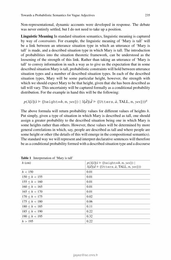
Towards a Probabilistic Semantics for Vague Adjectives 235
Non-representational, dynamic accounts were developed in response. The debatewas never entirely settled, but I do not need to take up a position.
Linguistic Meaning In standard situation semantics, linguistic meaning is capturedby way of constraints. For example, the linguistic meaning of ‘Mary is tall’ willbe a link between an utterance situation type in which an utterance of ‘Mary istall’ is made, and a described situation type in which Mary is tall. The introductionof probabilities into the situation theoretic framework, can be understood as theloosening of the strength of this link. Rather than taking an utterance of ‘Mary istall’ to convey information in such a way as to give us the expectation that in somedescribed situationMary is tall, probabilistic constraints will hold between utterancesituation types and a number of described situation types. In each of the describedsituation types, Mary will be some particular height, however, the strength withwhich we should expect Mary to be that height, given that she has been described astall will vary. This uncertainty will be captured formally as a conditional probabilitydistribution. For the example in hand this will be the following:
p(λ[s](s � 〈〈height=h,m, yes〉〉) | λ[d](d � 〈〈Utters, a,TALL,m, yes〉〉))g
The above formula will return probability values for different values of heights h.Put simply, given a type of situation in which Mary is described as tall, one shouldassign a greater probability to the described situation being one in which Mary issome heights rather than others. However, these values will be determined by moregeneral correlations in which, say, people are described as tall and where people aresome height or other (the details of this will emerge in the compositional semantics).The standard way we will represent and interpret declarative sentences will thereforebe as a conditional probability formed with a described situation type and a discourse
Table 1 Interpretation of ‘Mary is tall’
h (cm) p(λ[s](s � 〈〈height=h,m, yes〉〉) |λ[d](d � 〈〈Utters, a,TALL,m, yes〉〉))
h < 150 0.01
150 ≤ h < 155 0.01
155 ≤ h < 160 0.01
160 ≤ h < 165 0.01
165 ≤ h < 170 0.01
170 ≤ h < 175 0.02
175 ≤ h < 180 0.06
180 ≤ h < 185 0.11
185 ≤ h < 190 0.22
190 ≤ h < 195 0.32
h > 195 0.22
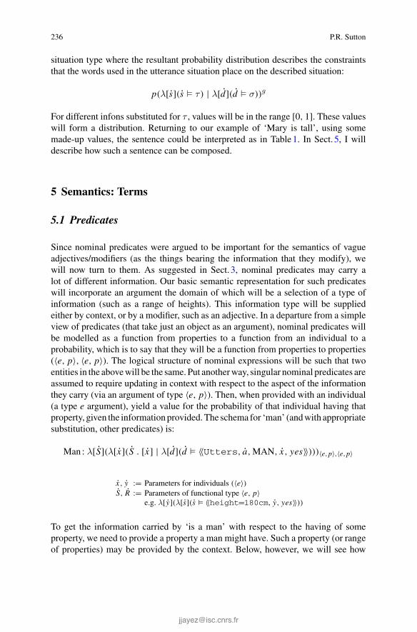
236 P.R. Sutton
situation type where the resultant probability distribution describes the constraintsthat the words used in the utterance situation place on the described situation:
p(λ[s](s � τ ) | λ[d](d � σ))g
For different infons substituted for τ , values will be in the range [0, 1]. These valueswill form a distribution. Returning to our example of ‘Mary is tall’, using somemade-up values, the sentence could be interpreted as in Table1. In Sect. 5, I willdescribe how such a sentence can be composed.
5 Semantics: Terms
5.1 Predicates
Since nominal predicates were argued to be important for the semantics of vagueadjectives/modifiers (as the things bearing the information that they modify), wewill now turn to them. As suggested in Sect. 3, nominal predicates may carry alot of different information. Our basic semantic representation for such predicateswill incorporate an argument the domain of which will be a selection of a type ofinformation (such as a range of heights). This information type will be suppliedeither by context, or by a modifier, such as an adjective. In a departure from a simpleview of predicates (that take just an object as an argument), nominal predicates willbe modelled as a function from properties to a function from an individual to aprobability, which is to say that they will be a function from properties to properties(〈e, p〉, 〈e, p〉). The logical structure of nominal expressions will be such that twoentities in the abovewill be the same. Put anotherway, singular nominal predicates areassumed to require updating in context with respect to the aspect of the informationthey carry (via an argument of type 〈e, p〉). Then, when provided with an individual(a type e argument), yield a value for the probability of that individual having thatproperty, given the informationprovided.The schema for ‘man’ (andwith appropriatesubstitution, other predicates) is:
Man : λ[S](λ[x](S . [x] | λ[d](d � 〈〈Utters, a,MAN, x, yes〉〉)))〈e,p〉,〈e,p〉
x, y := Parameters for individuals (〈e〉)S, R := Parameters of functional type 〈e, p〉
e.g. λ[y](λ[s](s � 〈〈height=180cm, y, yes〉〉))
To get the information carried by ‘is a man’ with respect to the having of someproperty, we need to provide a property a man might have. Such a property (or rangeof properties) may be provided by the context. Below, however, we will see how

Towards a Probabilistic Semantics for Vague Adjectives 237
part of the semantic contribution of predicate modifiers is to provide such a property(such a range of properties).
Because nominal predicates are functions from properties of described situationtypes to a function from individuals to a probability, a worry over tractability andlearnability arises. If an agent needs to learn all distributions that arise from interpret-ing ‘x is a man’ constructions, this would not be a tractable learning task. However,probabilistic learning affords a solution. We can assume that agents begin classifierlearning tasks with flat prior distributions for all collections of properties. On beingexposed to uses of a classifier, distributions will be adjusted for just those propertiesthe objects are perceived to have. In this sense, if one has no reasonable expectationsregarding some range of situations, given what has been said, simply because no onesituation type is more plausible than another, then it is possible that the classifierused does not carry information about (the properties in) those situations.19
One property a manmight have is of being a certain height. For example, he mightbe 180cm in height:
λ[y](λ[s](s � 〈〈height=180cm, y, yes〉〉))
This kind of property can be applied to our representation of the predicate ‘man’:
λ[S](λ[x](S . [x] | λ[d](d � 〈〈utters, a,MAN, x, yes〉〉) .
[λ[y](λ[s](s � 〈〈height=180cm, y, yes〉〉)]⇒λ[x](λ[y](λ[s](s � 〈〈height=180cm, y, yes〉〉) . [x] |
λ[d](d � 〈〈utters, a,MAN, x, yes〉〉)))⇒λ[x](λ[s](s � 〈〈height=180cm, x, yes〉〉 | λ[d](d � 〈〈utters, a,MAN, x, yes〉〉)
This is now in the right shape to take an individual as an argument which willbe described as a man in d and assigned the height property in s. Assuming (as asimplification) that names refer and carry no other information, this means that ‘Johnis a man’ can be represented, with respect to being 180cm in height, as follows20:
λ[s](s � 〈〈height=180cm,j, yes〉〉) | λ[d](d � 〈〈utters, a,MAN,j, yes〉〉)
The interpretation of this will be a probability value that reflects, with respect toJohn having some height, the probability of John having that height, given that hehas been described as a man.
19Of course, given particularly skewed learning data, anomalies in individuals semantic repre-sentations may occur. There will, nonetheless, be general patterns of use across whole languagecommunities. What learners are assumed to be implicitly doing is approximating to the patterns ofuse in their learning communities as a whole.20I ignore the contribution of the indefinite article and treat this as a simple predication. I leave themodelling of quantification in this system for future research.

238 P.R. Sutton
Of course, ‘John is a man’ will carry more information than this about John, butlet us focus on information carried about his height. We can consider the range ofheights John might be (given that he has been described as a man). There will be arationality constraint on the values ‘John is a man’ receives with respect to John’sheight. The values, must sum to 1. As a simplification, we may think in discretevalues, although a more accurate representation would be a continuous function.
Put anotherway, providingdifferent arguments of height properties for the formulaabovewill generate a probability distribution. Table2 shows one possible distributionfor the height information carried by ‘John is aman’ simplified over ranges of heights.
Describing John as a man, in part, conveys information about his height: that it isfairly probable that he is around average height and highly probable that he is neitherfar below nor far above average height. This relates to the assumption that learningthe classifier ‘man’, in part, involves learning, approximately, the ranges of heightsmen tend to come in. This needn’t be in centimetres. It need only be internalisedin such a way as to aid, to some extent, the ability to identify and classify whetherobjects in one’s environment are men.
TallAs a predicatemodifier, ‘tall’, when applied to a nominal predicate, increases our(reasonable) expectations of the entity (that predicate is applied to) having a greaterheight. ‘Tall’ will therefore be modelled as having two jobs to do when applied toa common noun like ‘man’: (i) it will pick out the information carried by ‘man’with respect to height. (ii) it will be a function on the probability distribution that‘man’ generates with respect to heights (it will make taller heights more probableand shorter heights less probable). In terms of a distribution curve, for a graph withprobabilities on its y-axis and heights on its x-axis, it would shift the whole curvealong the x-axis in the direction of greater heights. The representation of ‘tall’ isgiven below, along with a derivation for ‘tall man’.
Table 2 Interpretation of ‘John is a man’ with respect to height
h (cm) p(λ[s](s � 〈〈height=h,j, yes〉〉) |λ[d](d � 〈〈utters, a,MAN,j, yes〉〉))
h < 150 0.01
150 ≤ h < 155 0.04
155 ≤ h < 160 0.08
160 ≤ h < 165 0.12
165 ≤ h < 170 0.15
170 ≤ h < 175 0.20
175 ≤ h < 180 0.15
180 ≤ h < 185 0.12
185 ≤ h < 190 0.08
190 ≤ h < 195 0.04
h > 195 0.01

Towards a Probabilistic Semantics for Vague Adjectives 239
tall : λ[P](λ[y](C × ftall((P . [y]) . [(λ[z](s � 〈〈height=h, z, yes〉〉)]))))man : λ[S](λ[x]((S . [x] | d � 〈〈utters, a,MAN, x, yes〉〉)))tall man : λ[P](λ[y](C × ftall((P . [y])) . [(λ[z]s � 〈〈height=h, z, yes〉〉)])))) .
[λ[S]λ[x] (S . [x] | d � 〈〈utters, a,MAN, x, yes〉〉)]⇒ λ[y](C × ftall( λ[s](s � 〈〈height=h, y, yes〉〉) |
λ[d](d � 〈〈utters, a,MAN, y, yes〉〉)))
P := Parameter of type 〈〈e, p〉, 〈e, p〉〉 (functional type from situation properties to a functionfrom individuals to [0, 1])
C := Normalising valueftall := Expression of type 〈p, p〉
The interpretation of which is a function from individuals to a probability distri-bution for heights of that individual, given the individual’s description as a tall man.Whatever function on distributions ftall is, C will be interpreted as the value thatnormalises the distribution.21 One possible interpretation for f tall could be that it hasthe effect of shifting the distribution for ‘man’ up by 20cm or so (and stretching itvertically).22 In Table3, from the above toy distribution for ‘John is a man’, we canget a toy distribution for ‘John is a tall man’.23
Simply translated, being told that John is a manmay carry all sorts of information.Some of this is that he is more likely than not to be within some margin of average
Table 3 Interpretation of ‘man’, and ‘tall man’ (unnormalised and normalised) with respect toheight
h (cm) p(Φ) p( ftall(Φ)) p(C × ftall(Φ))
h < 150 0.01 0.01 0.01
150 ≤ h < 155 0.04 0.01 0.01
155 ≤ h < 160 0.08 0.01 0.01
160 ≤ h < 165 0.12 0.01 0.01
165 ≤ h < 170 0.15 0.01 0.01
170 ≤ h < 175 0.20 0.02 0.02
175 ≤ h < 180 0.15 0.06 0.06
180 ≤ h < 185 0.12 0.10 0.11
185 ≤ h < 190 0.08 0.20 0.22
190 ≤ h < 195 0.04 0.30 0.32
h > 195 0.01 0.20 0.22
21Which will be 1 over the sum of the modified distribution.22This could also be described by adjusting values of parameters on a Gaussian function.23I assume that 0.01 is the arbitrarily small value. Φ is an abbreviation for λ[s](s �〈〈height=h,j, yes〉〉 | d � 〈〈utters, a,MAN,j, yes〉〉).
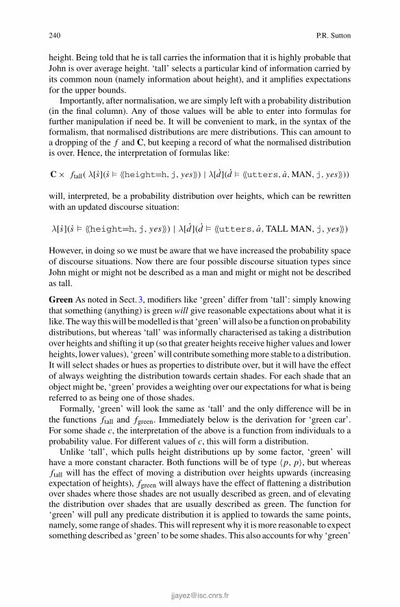
240 P.R. Sutton
height. Being told that he is tall carries the information that it is highly probable thatJohn is over average height. ‘tall’ selects a particular kind of information carried byits common noun (namely information about height), and it amplifies expectationsfor the upper bounds.
Importantly, after normalisation, we are simply left with a probability distribution(in the final column). Any of those values will be able to enter into formulas forfurther manipulation if need be. It will be convenient to mark, in the syntax of theformalism, that normalised distributions are mere distributions. This can amount toa dropping of the f and C, but keeping a record of what the normalised distributionis over. Hence, the interpretation of formulas like:
C × ftall( λ[s](s � 〈〈height=h,j, yes〉〉) | λ[d](d � 〈〈utters, a,MAN,j, yes〉〉))
will, interpreted, be a probability distribution over heights, which can be rewrittenwith an updated discourse situation:
λ[s](s � 〈〈height=h,j, yes〉〉) | λ[d](d � 〈〈utters, a,TALL MAN,j, yes〉〉)
However, in doing so we must be aware that we have increased the probability spaceof discourse situations. Now there are four possible discourse situation types sinceJohn might or might not be described as a man and might or might not be describedas tall.
Green As noted in Sect. 3, modifiers like ‘green’ differ from ‘tall’: simply knowingthat something (anything) is green will give reasonable expectations about what it islike. Theway thiswill bemodelled is that ‘green’will also be a function onprobabilitydistributions, but whereas ‘tall’ was informally characterised as taking a distributionover heights and shifting it up (so that greater heights receive higher values and lowerheights, lower values), ‘green’will contribute somethingmore stable to a distribution.It will select shades or hues as properties to distribute over, but it will have the effectof always weighting the distribution towards certain shades. For each shade that anobject might be, ‘green’ provides a weighting over our expectations for what is beingreferred to as being one of those shades.
Formally, ‘green’ will look the same as ‘tall’ and the only difference will be inthe functions ftall and fgreen. Immediately below is the derivation for ‘green car’.For some shade c, the interpretation of the above is a function from individuals to aprobability value. For different values of c, this will form a distribution.
Unlike ‘tall’, which pulls height distributions up by some factor, ‘green’ willhave a more constant character. Both functions will be of type 〈p, p〉, but whereasftall will has the effect of moving a distribution over heights upwards (increasingexpectation of heights), fgreen will always have the effect of flattening a distributionover shades where those shades are not usually described as green, and of elevatingthe distribution over shades that are usually described as green. The function for‘green’ will pull any predicate distribution it is applied to towards the same points,namely, some range of shades. This will represent why it is more reasonable to expectsomething described as ‘green’ to be some shades. This also accounts for why ‘green’
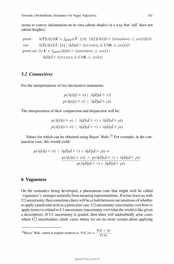
Towards a Probabilistic Semantics for Vague Adjectives 241
seems to convey information on its own (about shades) in a way that ‘tall’ does not(about heights).
green: λ[P](λ[y](C × fgreen((P . [y]) . [λ[z](λ[s](s � 〈〈shade=c, z, yes〉〉)]))))car: λ[S](λ[x](S . [x] | λ[d](d � 〈〈utters, a,CAR, x, yes〉〉)))green car: λy.C × fgreen(λ[s](s � 〈〈shade=c, y, yes〉〉) |
λ[d](d � 〈〈utters, a,CAR, y, yes〉〉))
5.2 Connectives
For the interpretations of two declarative statements:
p(λ[s](s � σ) | λ[d](d � τ ))
p(λ[s](s � σ) | λ[d](d � ρ))
The interpretation of their conjunction and disjunction will be:
p(λ[s](s � σ) | λ[d](d � τ ) ∧ λ[d](d � ρ))
p(λ[s](s � σ) | λ[d](d � τ ) ∨ λ[d](d � ρ))
Values for which can be obtained using Bayes’ Rule.24 For example, in the con-junction case, this would yield:
p(λ[s](s � σ) | λ[d](d � τ ) ∧ λ[d](d � ρ)) =p(λ[s](s � σ)) ∧ p(λ[d](d � τ ) ∧ λ[d](d � ρ))
p(λ[d](d � τ ) ∧ λ[d](d � ρ))
6 Vagueness
On the semantics being developed, a phenomena (one that might well be called‘vagueness’), emerges naturally frommeaning representations. If terms leave us withU2uncertainty, then sometimes therewill be a clash betweenour intuitions ofwhetherto apply a particular term in a particular case. U2 uncertainty (uncertainty over how toapply terms) is related toU1 uncertainty (uncertainty overwhat theworld is like givena description). If U1 uncertainty is graded, then there will undoubtedly arise caseswhere U2 uncertainties clash: cases where we are no more certain about applying
24Bayes’ Rule, stated in regular notation is: P(C |A) = P(C ∧ A)
P(A).
242 P.R. Sutton
a term than we are about applying its negation. Furthermore, some cases of clasheswill be immune to further information. One could be in a position of full knowledgesuch that one knew exactly how words were used, all of the relevant properties of theobjects being described, and all of the relevant contextual information. Nonetheless,clashes of equal uncertainty may remain unresolved. Such situations, I contend, areplausible explanations of so-called borderline cases.
For example, if the value for ‘John is tall’ with respect to height h is the sameas the value for ‘John is not tall’ with respect to height h, then the meaning of ‘tall’will provide us with no more reason to judge John to be tall than to judge him to benot tall. There is no more to know about the meaning of ‘tall’ which will resolve thisuncertainty, and there may be no more to know about John or the context of utteranceto do so either. If so, John would be a borderline case.
Probability values in the formalism can be seen to reflect reasons for makingjudgements. In viewing matters this way, we can begin to get a handle on bound-arylessness. Even if our reasons for making a ‘tall’ judgement slightly outweigh ourreasons for making a ‘not tall’ judgement, we might still not have sufficient reason toform a categorical judgement. The extent to which the values must differ for one orthe other judgement to be true will not be a matter decided by the semantics for ‘tall’.In this sense, nothing in the meaning representation itself will determine a cut-offpoint for ‘tall’. It is due to this feature of the model provided that we can approximateboundarylessness for vague concepts.
7 Comparison with the Literature
7.1 Lassiter’s, and Frazee and Beaver’s Epistemic Models
Although Lassiter (2011) and Frazee and Beaver (2010) describe their positions fromdifferent perspectives, they amount to similar approaches. Lassiter’s article, thoughmarginally later was developed independently and is fuller in detail. I will focus onit.
Similarly to my approach, Lassiter is interested in uncertainty in communicationand worried about sharp boundaries. Rather than implementing probabilities directlyinto the meaning representations of words, Lassiter incorporates metalinguisticuncertainty over what is being expressed (in terms of a sharp proposition). He alsoincludes uncertainty about the world, but we’ll focus on the former case.
Lassiter inherits, from other work in the scalar adjectives literature, the idea thattheir semantics should incorporate thresholds. In simple terms, hemodels uncertaintyabout where the threshold is when a term like ‘tall’ is used. We can, relative to acontext, be pretty certain that thresholds are not too high or too low. Lassiter modelsthis as a distribution over precise model theoretic objects which have sharp cut-offs.The effect is that if we learn someone’s height, we can get a value that reflects theprobability that individual is tall.

Towards a Probabilistic Semantics for Vague Adjectives 243
However, Lassiter’s emphasis is not on the sharp boundaries that such a posi-tion implies. For him (and for Frazee and Beaver), communication using ‘tall’ isabout approximating, roughly, the standard in play for what would count as tall. It isthese standards that we are uncertain about when someone uses the expression ‘tall’.However, this general picture has the effect of implying that there is, nonetheless, astandard for ‘tall’ in every context. I have suggested that the approximation of stan-dards is not what is encoded by our words. This amounts to the claim that uncertaintyshould enter at the level of describing the model theoretic object, not at the level ofevaluating which classical model theoretic object is in play.
Lassiter’s account is a big improvement on standard non-probabilistic approaches.However, the fact remains that themotivation for appealing to precise languagesmuststill be given. If it turns out that we rarely, if ever, coordinate sufficiently to settleon exactly where a threshold for ‘tall’ should be, then why have such thresholdswritten so centrally into the semantics of such terms? We can drop precise lan-guages and have a far more direct connection to what our terms mean by adoptingthe picture proposed.
7.2 Cooper et al.’s Probabilistic Type-Theoretic Approach
Semantic learning is at the forefront of Cooper et al. (2014), which is also the closestposition to my own. I strongly suspect that the core of the two positions will be prettyinter-definable, although there are differences of emphasis.
U1 uncertainty is uncertainty about the world, given a description of it. U1 uncer-tainty is, effectively, what my account describes. Arguably, Cooper et al. focus onU2 uncertainty. U2 uncertainty is uncertainty about how to use words, given someknown or perceived way the world is. I will say more about Cooper et al. formal-ism in a moment, but it is first worth remarking that, if modelled as I have pre-sented, U1 and U2 uncertainty are inter-definable. The main weight of the mean-ings of utterances in my account rests on conditional probabilities of the formp(λ[s](s � σ)|λ[d](d � τ )). In other words, the probability of the world beingsome way, given a description of it. If, indeed, Cooper et al.’s account describes U2uncertainty, then it is possible that their results could be simulated via the use of thealternate conditional probability: p(λ[d](d � τ )|λ[s](s � σ)) (or the probability thatsome description will be used, given that the world is some way). Importantly, giventhe priors p(λ[s](s � σ)) and p(λ[d](d � τ )), these two conditional probabilitiesare simply ratios of each other.
Cooper et al.’s semantics uses a rich theory of types. The simple type theory Ihave used provided domains for basic types. Complex types were then constructedas functions of basic types. In rich type theories, types should not be thought ofin these extensional terms, but instead as something like useful ways of classifyingthings (Cooper 2012, p. 275). However, propositions are also types. For example,the proposition David runs can be seen as a situation type (one in which David runs),and is true iff there is a situation in the world in which David runs. In Cooper et al.
244 P.R. Sutton
(2014) agents are modelled asmaking probabilistic judgements about classifications.Propositions are still types, but judgements reflect the probabilities that there is asituation of the right type.
Of particular interest is how these type judgements are grounded. Central toCooper et al.’s account is semantic learning, a wider discussion of which featuresin Cooper et al. (2013). On their learning model, a learner is exposed to multiplesituations. In each one they make a judgement about whether the object they areshown is an apple or not an apple. After each judgement, the oracle that modelsthe adult speaker gives a judgement. Initially, the learner cannot make a judgement,but after a few exposures to adult judgements, has enough data to begin to makejudgements herself. In Cooper et al.’s model, ‘apple’ judgements are based on fourproperties (two colours and two shapes). Simplifying a little, when faced with a newobject to classify, the value of the judgement is calculated as the conditional proba-bility p(apple|observed properties).25 To calculate that conditional probability, thelearner uses priors and conditional probabilities such as p(property|apple), both ofwhich are estimated directly from the adult judgements she have witnessed.
Translating more into my own vernacular, one could see probabilities of ‘apple’judgements as approximating probabilities of discourse situations, and we could seeprobabilities of properties as approximating probabilities of described situations. Thetwo stages of Cooper et al. learning account can then be described with the followingprocedure:
(i) By directly witnessing adult speakers’ linguistic behaviour, estimate probabili-ties of the form:p(λ[s](s � 〈〈colourc, x, yes〉〉)), p(λ[s](s � 〈〈shapes, x, yes〉〉)),p(λ[d](d � 〈〈utters, a,APPLE, x, yes〉〉)),p(λ[s](s � 〈〈colourc, x, yes〉〉)|λ[d](d � 〈〈utters, a,APPLE, x, yes〉〉)), andp(λ[s](s � 〈〈shapes, x, yes〉〉)|λ[d](d � 〈〈utters, a,APPLE, x, yes〉〉)).
(ii) Use those values to calculate, of a novel object/context, the probability:p[λ[d](d � 〈〈utters, a,APPLE, x, yes〉〉))|λ[s]s � 〈〈colourc, x, yes〉〉 ∧ λ[s]s � 〈〈shapes, x, yes〉〉).
The process in (i) describes learning the kinds of meaning representations I haveproposed. Cooper et al. show how the kind of information that can be learnt fromadult speakers’ linguistic behaviour can be turned into a classifier judgement. Thesejudgements will not always be probability 1. The uncertainty that <1 judgementsreflect, is, Iwould argue, justwhat I described asU2uncertainty.Acloser examinationof the two accounts could be fruitful. It would certainly be useful if I were simplyable to adopt Cooper et al. learning model.
25Where the output judgement is decided bywhether an ‘apple’ or an ‘not-apple’ judgement receivesa higher value.
Towards a Probabilistic Semantics for Vague Adjectives 245
One distinct contribution the account in this paper makes is in the treatment ofadjectives. Cooper et al.’s learning account shows howanominal like ‘apple’ could belearnt from basic colour and shape observations. I have argued that vague modifiersshould be viewed as functions on distributions given by nominal classifiers.
8 Conclusions
Situation theory captures sentence meaning as a link between discourse situationtypes and described situation types. Although the way that this idea has been devel-oped here differs from the situation theoretic account in many ways, the basic spiritof the account remains. On the standard view, informational links hold between sit-uation types. Individuals build connections with the world via learning (learning todecode the information carried by terms) and via communication. The reproductionof expressions for similar purposes entrenches these relations.
On the account presented here, the meanings of expressions are correlationalinformational links between discourse situation types and described situation typesthat arise from patterns in language use. People connect to these correlations viasemantic learning, and they entrench correlations via reproduction of language torefer to similar situations.
Vagueness naturally arises from modelling such relations probabilistically. Thiscan be viewed either as the boundarylessness of vague predicates achieved by sep-arating, or at least distancing, truth conditions from semantic representations, or asborderline cases, where the meaning of a term such as ‘tall’ can provide competingreasons to make ‘tall’ and ‘not tall’ judgements.
However, the suggestions put forward here are rather programmatic and manyissues have remained entirely unaddressed. Nonetheless, at least for vague terms,structured, probabilistic representations of meaning provide at least one viable routefor attempting to capture the boundarylessness that seems characteristic of vagueness.
Acknowledgments I would like to thank the organisers and participants of the Bayesian NaturalLanguage Semantics and Pragmatics workshop held at ESSLLI 2013 and the anonymous reviewersfor the workshop and this volume for the helpful comments and improvements that they havesuggested. Thanks also to the participants of the King’s College London Language and CognitionSeminar, with special thanks to Alex Clark, Ruth Kempson, Shalom Lappin, and Wilfried Meyer-Viol for their invaluable comments on earlier versions of this paper.
References
Barwise, J., & Perry, J. (1983). Situations and attitudes. Stanford: CSLI.Cooper, R., Dobnik, S., Lappin, S., & Larsson, S. (2013). Probabilistic type theory and naturallanguage semantics (manuscript) University of Gothenburg and King’s College London.

246 P.R. Sutton
Cooper, R., Dobnik, S., Lappin, S., & Larsson, S. (2014). A probabilistic rich type theory forsemantics interpretation. InProceedings of the EACL 2014 Workshop on Type Theory and NaturalLanguage Semantics, Gothenburg.
Cooper, R. (1996). The role of situations in generalised quantifiers. In S. Lappin (Ed.),The handbookof contemporary semantic theory (pp. 65–86). Cambridge: Blackwell.
Cooper, R. (2012). Type theory and semantics in flux. In R. Kempson, T. Fernando, & N. Asher(Eds.), Philosophy of linguistics Handbook of the philosophy of science, (vol. 14, pp. 271–323).Oxford: Elsevier.
Cresswell, M. J. (1974). The semantics of degree. In B. Partee (Ed.), Montague grammar (pp.261–292). New York: Academic Press.
de Marnee, M., Manning, C.D., & Potts, C. (2010). Was it good? It was provocative. Learning themeaning of scalar adjectives. In Proceedings of the 48th Annual Meeting of the Association forComputational Linguistics (pp. 167–176). Stroudsberg, ACL.
Devlin, K. (2006). Situation theory and situation semantics. In D. Gabbay & J. Woods (Eds.),Handbook of the history of logic (Vol. 7, pp. 601–664). Amsterdam: Elsevier.
Frazee, J., & Beaver, D. (2010). Vagueness is rational under uncertainty. InM. Aloni, H. Bastiaanse,T. de Jager, & K. Schulz (Eds.), Logic, language and meaning: 17th Amsterdam colloquium,Amsterdam, The Netherlands, December 16–18, 2009, Revised Selected Papers. LNAI (Vol. 6042,pp. 153–162). Heidelberg: Springer.
Gargett, A., Gregoromichelaki, E., Kempson, R., Purver, M., & Sato, Y. (2009). Grammar resourcesfor modelling dialogue dynamically. Cognitive Neurodynamics, 3, 347–363.
Graff Fara, D. (2000). Shifting sands: An interest relative theory of vagueness.Philosophical Topics,28(1), 45–81.
Kamp, H. (1975). Two theories about adjectives. In E. Keenan (Ed.), Formal semantics of naturallanguage (pp. 123–155). Cambridge: Cambridge University Press.
Kamp, H., & Reyle, U. (1993). From discourse to logic. Dordrecht: Kluwer.Kennedy, C. (1997). Projecting the adjective: The syntax and semantics of gradability and compar-ison. Ph.D. Thesis, University of California, Santa Cruz.
Kennedy, C. (2007). Vagueness and grammar: The semantics of relative and absolute gradableadjectives. Linguistics and Philosophy, 30(1), 1–45.
Kolmogorov, A. (1950). Foundations of probability. New York: Chelsea Publishing.Lassiter, D. (2011). Vagueness as probabilistic linguistic knowledge. In R. Nouwen, U. Sauerland,H. C. Schmitz, & R. van Rooij (Eds.), Vagueness in communication. LNAI (Vol. 6517, pp. 127–150). Heidelberg: Springer.
Sainsbury, R. M. (1991). Concepts without boundaries, Inaugural Lecture. King’s College London,London. Reprinted. In R. Keefe, P. Smith (Eds.), Vagueness: A reader (pp. 251–264). MIT Press,Cambridge (1996).
Sutton, P. R. (2013). Vagueness, communication and semantic information. King’s College London.Ph.D. Thesis.