Embed Size (px)
Citation preview
Computer-Aided Civil and Infrastructure Engineering 00 (2014) 1–17
Bayesian Modeling of External Corrosion inUnderground Pipelines Based on the Integrationof Markov Chain Monte Carlo Techniques and
Clustered Inspection Data
Hui Wang, Ayako Yajima & Robert Y. Liang*
Department of Civil Engineering, The University of Akron, Akron, OH, USA
&
Homero Castaneda
Department of Chemical and Biomolecular Engineering, National Center for Research in Corrosion and MaterialsPerformance, The University of Akron, Akron, OH, USA
Abstract: In this study, a model is developed to assessexternal corrosion in buried pipelines based on the uni-fication of Bayesian inferential structure derived fromMarkov chain Monte Carlo techniques using clusteredinspection data. This proposed stochastic model com-bines clustering algorithms that can ascertain the simi-larity of corrosion defects and Monte Carlo simulationthat can give an accurate probability density function es-timation of the corrosion rate. The metal loss rate is cho-sen as the indicator of corrosion damage propagation,obeying a generalized extreme value (GEV) distribution.Bayesian theory was employed to update the probabilitydistribution of metal loss rate as well as the GEV param-eters in order to account for the model uncertainty. Theproposed model was validated with direct and indirectinspection data extracted from a 110-km buried pipelinesystem.
1 INTRODUCTION
Steel pipelines are widely used for oil transportationin the petroleum industry. Usually, these metallic lon-gitudinal structures are buried underground. Because
To whom correspondence should be addressed. E-mail: [email protected].
they are directly exposed to aggressive soil and under-water environments, different protection systems areadded to the structure: one system uses direct protec-tion by incorporating physical barriers (such as coat-ings), and a second employs an external source (suchas cathodic protection). These systems can be classifiedas preventative or as mitigation. Unfortunately, neitherof these protection systems is completely reliable forsafeguarding an operating pipeline, as various circum-stances can decrease the performance of these systemsand produce risk factors leading to failure conditions(Abes et al., 1985). Excavation damage to the pipeline,fouling of coatings, or electrochemically triggered pro-cesses that cause coating failure can be some initiatorsfor corrosion activation. Cathodic protection is an ex-ternal source that is a function of the environment (soil)and can contribute to damage evolution of the coatingat any particular location. The corrosion process can beactivated under protection conditions depending on theenvironment and the degree of damage. Hence, exter-nal localized corrosion is one of the most common de-fects that occurs under normal operating conditions of apipeline (Peabody et al., 2001).
The severity of the external corrosion process canbe evaluated by quantifying the rate of local damageevolution propagation. A number of studies (DeWaard
C© 2014 Computer-Aided Civil and Infrastructure Engineering.DOI: 10.1111/mice.12096
2 Wang, Yajima, Liang & Castaneda
and Milliams, 1975; Engelhardt et al., 1999; Anderkoet al., 2001) have developed models in order to esti-mate the corrosion rate using basic variables such aspH, pressure, temperature, and concentration of ions(i.e., Cl−, SO4
2−, OH−). The limitation of these mod-els is that they are only valid under laboratory condi-tions. Melchers (2003) developed a phenomenologicalmodel for general corrosion of mild and low-alloy steelsunder fully aerated condition in marine environment.For in situ or noncontrolled situations, however, thereis a lack of knowledge about all the factors contribut-ing to corrosion propagation. In addition, the pipelineis exposed to a dynamic aggressive environment duringthe years of its operation, and the factors affecting thecorrosion process will change continuously over time.From a dynamic (time-dependent) perspective, the cor-rosion rate must be considered as a random variable un-der field conditions, and it can be predicted from theperspective of probability (Shibata, 1996; Alamilla andSosa, 2008; Caleyo et al., 2009b). On the other hand, atsites where the inspection or monitoring tools indicatethat the corrosion rate is extremely high, the parametersassociated with corrosion process are difficult to quan-tify deterministically. Furthermore, it is relatively diffi-cult (and sometimes impossible) to predict the extremevalue using a traditional physical model. Hence, uncer-tainties should be given significant attention when esti-mating the corrosion propagation.
To the best of the authors’ knowledge, only a fewstochastic models can be used to predict the externalcorrosion rate in underground pipelines in terms ofprobability and to perform risk analysis (Hong, 1999;Sinha and Pandey, 2002; Kiefner and Kolovich, 2007;Race et al., 2007; Alamilla and Sosa, 2008; Caleyo et al.,2009a). Hong (1999) took the effect of the generation ofnew defects into consideration on the reliability estima-tion and the corrosion effect on pipeline was modeledby a Markov process. Alamilla et al. (2008) proposed astochastic method that contains four models to estimatethe corrosion propagation rate. The probability distri-butions of the corrosion depth and corrosion rate arederived analytically, based on the empirical distributionof the corrosion depth, the number of corrosion defects,and the distribution of the starting time. Some limita-tions to the previous models are the lack of consider-ation of soil properties due to environmental changesas well as evidence of the distribution of starting time.Kiefner and Kolovitch (2007) developed a Monte Carloapproach for estimating the probability distribution ofthe corrosion rate. In order to produce the probabilitydensity function (PDF) of the corrosion rate, sampleswere drawn from the depth and starting time distribu-tion to perform the Monte Carlo simulation. The resultswere very sensitive to the distribution of the corrosion
starting time. Caleyo et al. (2009a) developed the prob-ability distribution of pitting corrosion depth and ratein underground pipelines using Monte Carlo simulation.The investigation was based on a field study (Velazquezet al., 2009). The corrosion rate formula derived fromthe field study is a power law formulation of local en-vironmental factors. The statistic characters of the en-vironmental factors which were used as the inputs forthe Monte Carlo simulation were obtained by soil de-terminations. The limitation of this model is that thelinear assumption between the soil properties and theparameters in the power law formulation could be toostrong.
Technically, the pit depth or metallic indications at agiven time can be measured by in-line inspection (ILI)devices or can be estimated from direct observation ofa high number of excavations. The measurement of cor-rosion defects may be imprecise due to imperfect per-formance of operator and device as well as noise affect-ing measured signals (Maes et al., 2009; Sahraoui et al.,2013). The soil properties (half-cell potential, resistiv-ity, pH, concentration of ions, and soil moisture) can bemeasured via analytical and titration methods by tak-ing in situ samples along the pipeline at equal intervals.Hence, the information of soil environment is spatiallydiscrete.
In this work, we employ sampling, characterization,and analysis for soil properties along the right-of-way ofoil pipeline. For purposes of data analysis, the pipelineis divided into equal segments so that the physical andchemical properties are position-dependent. The corro-sion rate is considered to be under steady-state condi-tions. Each segment has a set of variables which arereferred to as features containing soil properties andoperation conditions. All the features form a high-dimensional feature space; within the feature space,each segment is represented by a vector. Clusteringtechniques should be employed to classify the segments,as the segments within each cluster will have high simi-larity in feature space. The similarity can be interpretedby a measure of distance (Ghosh-Dastidar and Adeli,2003; Jain, 2010), a probability density (Fraley andRaftery, 1998; Ahmadlou and Adeli, 2010; Kodogianniset al., 2013), or a graph (Bello-Orgaz et al., 2012;Menendez et al., 2014). Because of the high similarity,we can easily find the statistical property of each clus-ter and estimate the probability distribution of corro-sion rate within each cluster, this is the practical ad-vantage of the present work. Some of the most recentclustering techniques are well reported in the literature(Kodogiannis et al., 2013; Peng and Ouyang, 2013; Rizziet al., 2013; Menendez et al., 2014).
In this article, we propose a methodology based onclustering of the segments followed by the estimation
Bayesian modeling of external corrosion in underground pipelines 3
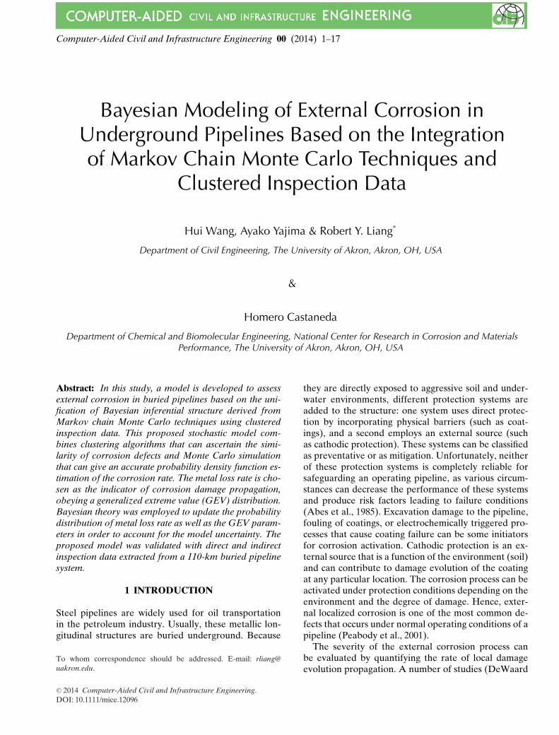
Clustering Process
Bayesian Inferential Framework (MCMC)
Start
PDF of metal loss rate at a certain location along pipeline
GEV parameter estimation of each cluster Site feature
End
Fig. 1. Flowchart of modeling procedure.
of the probability distribution parameters of the cor-rosion rate within each cluster using Bayesian inferen-tial framework. We obtain the boundary distribution ofthe metal loss rate for each cluster; then generalize theBayesian approach to estimate the probability distribu-tion of the corrosion rate at a specific site. The pro-posed method is able to interpret model uncertainty,which allows the upper and lower boundary distributionof the corrosion rate to be estimated. By the integra-tion of clustering algorithm and Markov chain MonteCarlo (MCMC) techniques, the proposed method canestimate corrosion rate at a specified location alongpipeline, which is the methodological advantage. Theproposed method is developed by validating in-line in-spection data and by performing in situ soil propertymeasurement sampling and quantification for each 200meters along a 110-km pipeline. The modeling flowchartis shown in Figure 1.
2 MODEL FRAMEWORK
2.1 Indicator of corrosion damage propagation
As is well known by both experiment (Szklarska-Smialowska, 1986) and theory (Engelhardt et al., 1999,2003, 2004) for localized corrosion, the defect character-istic dimension (e.g., the depth of the corrosion pitting)can be expressed by Equation (1)
D = ktα (1)
where k and α are empirical constants; usually, α � 1.And t is the time.
Based on Equation (1), the corrosion velocity is de-rived by the equation below
V = dD
dt= kαtα−1 (2)
In general, this expression shows the nonlinear trendof the corrosion damage propagation: the corrosion rateis relatively high at the beginning of the damage processand attenuates gradually as the service age increases.This function shows a nonphysical limit.
V = dD
dt= kαtα−1 →∞, at t → 0 (3)
Such a high-corrosion rate is impossible. Instead ofEquation (2), an equation proposed by Engelhardt andMacdonald (2004) can be applied to estimate the corro-sion rate:
V = dD
dt= V0
(1+ t
t0
)α−1
(4)
where V0 is the initial corrosion rate, and t0 is constantwhich has the effect on the time interval for reaching astable corrosion rate.
The corrosion behavior reflected in Equation (4) con-siders the early stages of corrosion, when the metalis exposed to a relatively high concentration of corro-sive species. As the exposure time increases, an oxidefilm forms on the corrosion defect surface, which canserve as a protective barrier against further corrosion(Bockris and Reddy, 1970). By assuming the corrosionproduct as being a stable passive layer, we can considerthat the corrosion rate is constant following the forma-tion of this layer.
During operation conditions, the depth and locationof an indicator of possible corrosion can be measuredand determined via magnetic flux leakage (MFL) or ul-trasonic tools (UTs). It is highly impractical to apply thetechnology to obtain initial corrosion velocity V0, sinceit is very costly to perform a direct inspection, and in-spections are typically scheduled at different time in-tervals. Theoretically, by using the measured corrosiondepth �D at inspection interval �t, the average corro-sion velocity can be estimated as
V = �D
�t(5)
One of the problems in using Equation (5) to obtainthe corrosion rate is that we need to identify the samedefect in two consecutive inspection results. This iden-tification is relatively difficult, as current technology isnot accurate enough to give an exact match of a corro-sion defect in two consecutive inspections (Westwoodand Hopkins, 2004).
4 Wang, Yajima, Liang & Castaneda
0 10 20 30 40 500
0.2
0.4
0.6
0.8
1
Service Life (year)
Met
al L
oss
Rat
e (m
m/y
ear) Metal Loss Rate
Fitted Mean Line
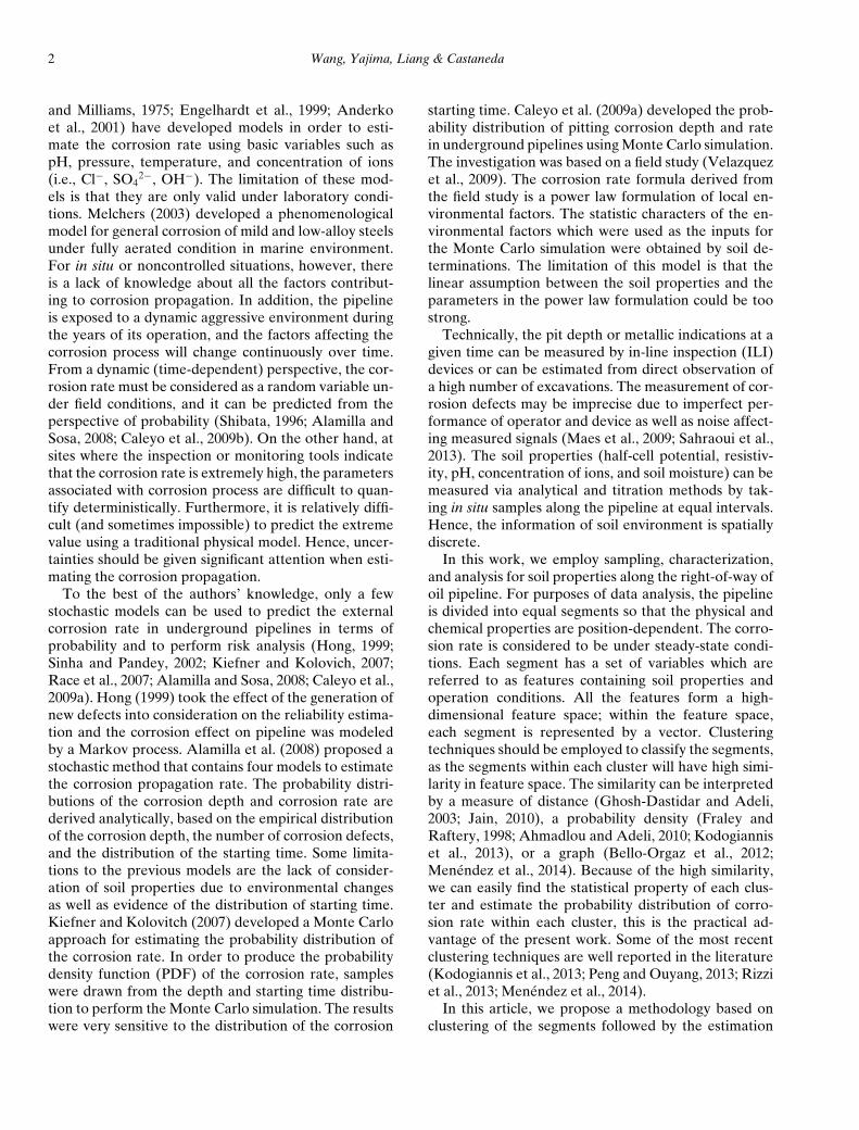
Fig. 2. The metal loss rate calculated by Equation (6) forentire 110-km length of pipeline.
A logical way to obtain the corrosion rate is to usethe inspection data and the service age, since corrosionis a dynamically stable process if there are no suddenchanges that radically affect the factors influencing pro-cess kinetics. Also, the localized critical pit depth (e.g.,the wall thickness of a pipeline) and the typical servicelife will impose a significant restriction on the initial andaverage corrosion current (Engelhardt and Macdonald,2004). Hence, considering the corrosion process as sta-ble and relatively slow, we can use the metal loss rate asan indicator of corrosion damage propagation, which isdefined by Equation (6)
r = D(t)t
(6)
where D(t) is the inspection data (the corrosion depth ofdefect) and t is the service life (from installation to thetime of inspection before replacement) of the pipelinesegment.
Based on the measurement profile of the defect fromin-line inspections and the service life obtained fromthe maintenance history along a 110-km pipeline, wecalculated the metal loss rate at each defect usingEquation (6) and plotted a curve that shows the trendin metal loss rate as the pipeline ages in Figure 2.
Figure 2 shows the correlation between metal lossrate and service life. From the inspection profile, wenotice that the trend is the same as Equation (4), witha high corrosion rate at the beginning and a slowingdue to the formation of a passive oxide film. As can beseen in Figure 2, after 29 years, the metal loss rate isnearly constant. For the convenience of statistical anal-ysis and incorporating as many samples as possible intothe stochastic analysis, we consider the metal loss rateto be constant after 29 years.
2.2 Clustering algorithm
The inspection data (metal loss rate) is clustered intogroups based on similarity in environmental informa-tion, which contains several critical parameters, by usingthe Gaussian mixture model (GMM) to extract under-lying patterns in the feature space (where all the crit-ical parameters form a feature space) and to improvethe accuracy of the estimation and the prediction of therate of metal loss. To avoid a natural clustering problem(Pang-Ning et al., 2006), we adopted expert opinions toassist in choosing the relevant corrosion factors. In thiswork, there are nine corrosion factors: distance fromthe nearest cathodic protection station to the defect,half-cell potential, soil resistivity, pH, four different ionconcentrations (CO3
2−, HCO3−, Cl−, SO4
2−), and soilmoisture. The GMM is evaluated with the expectation-maximization (EM) algorithm, which is a method forfinding the maximum likelihood function by optimiz-ing the parameters under hidden conditions (Ben-Huret al., 2002; Fraley and Raftery, 2002). The result is com-pared to K-means algorithm clusters that have been pre-viously reported by Jain (2010).
The difficulty in using clustering models is apparentwhen optimizing a number of clusters having a largedissimilarity between clusters while achieving a largesimilarity within each cluster. Several studies have beenperformed on model selection such as the Akaike infor-mation criterion (AIC), the Bayesian information cri-teria (BIC) (Fraley and Raftery, 1998), neural networkmethods (Lam et al., 2006; Adeli and Panakkat, 2009),and Bayesian approach combined with Monte Carlo in-tegration (Yuen and Mu, 2011). The BIC is more suit-able for high-dimensional data because it considers thefeature dimension by including it as a penalty (Fraleyand Raftery, 1998, 2002). Therefore, in this study, BICis used because of the multidimensional data structure.
In the GMM, the environmental information of asegment can be considered as a feature vector xi =(x1, x2, . . . , xd) in feature space. All the data are as-sumed to be generated by a mixture of normal probabil-ity density. Thus, we can calculate the likelihood of theobservations:
L(α, θ |x) =n∏
i=1
K∑j=1
α j f j (xi |θ j ) (7)
where α j is the mixing probability of jth cluster suchthat
∑kj=1 α j = 1, n is the number of observations, K
is the number of components, and f j (xi |θ j ) is a mul-tivariate normal distribution of d-dimension with pa-rameters θ j = (μ j ,� j ) where μ is a vector which con-tains the mean of every feature and � is the covariance
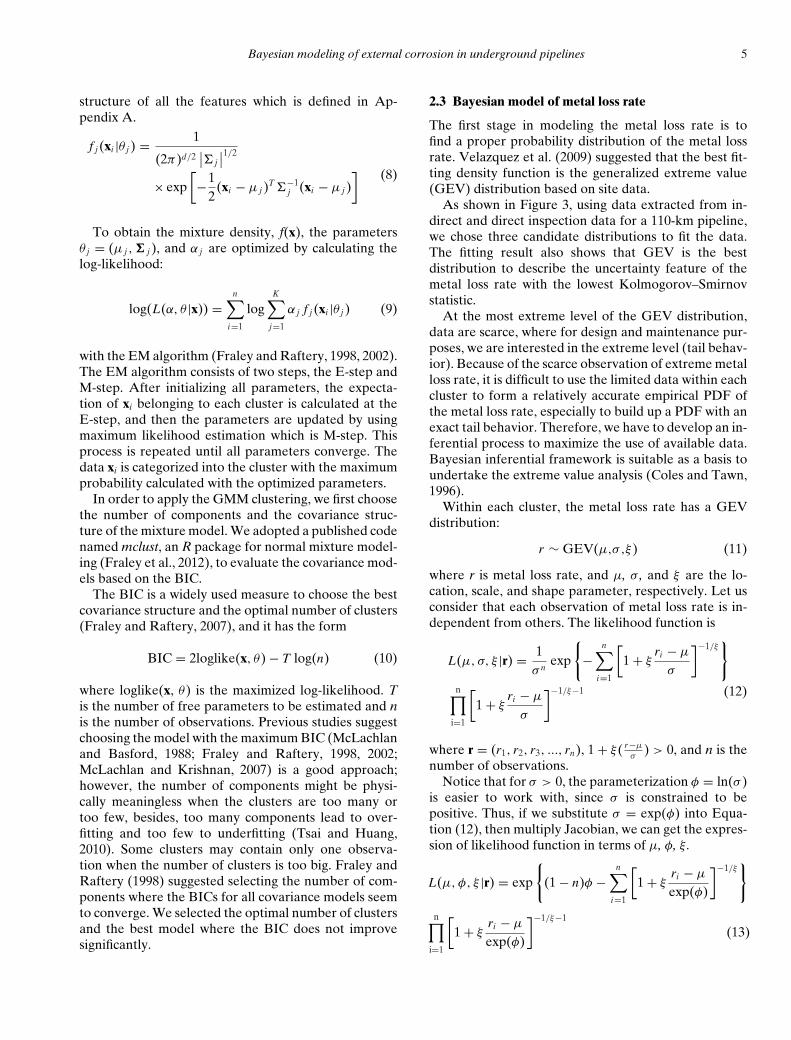
Bayesian modeling of external corrosion in underground pipelines 5
structure of all the features which is defined in Ap-pendix A.
f j (xi |θ j ) = 1
(2π)d/2∣∣� j
∣∣1/2
× exp[−1
2(xi − μ j )T �−1
j (xi − μ j )] (8)
To obtain the mixture density, f(x), the parametersθ j = (μ j ,� j ), and α j are optimized by calculating thelog-likelihood:
log(L(α, θ |x)) =n∑
i=1
logK∑
j=1
α j f j (xi |θ j ) (9)
with the EM algorithm (Fraley and Raftery, 1998, 2002).The EM algorithm consists of two steps, the E-step andM-step. After initializing all parameters, the expecta-tion of xi belonging to each cluster is calculated at theE-step, and then the parameters are updated by usingmaximum likelihood estimation which is M-step. Thisprocess is repeated until all parameters converge. Thedata xi is categorized into the cluster with the maximumprobability calculated with the optimized parameters.
In order to apply the GMM clustering, we first choosethe number of components and the covariance struc-ture of the mixture model. We adopted a published codenamed mclust, an R package for normal mixture model-ing (Fraley et al., 2012), to evaluate the covariance mod-els based on the BIC.
The BIC is a widely used measure to choose the bestcovariance structure and the optimal number of clusters(Fraley and Raftery, 2007), and it has the form
BIC = 2loglike(x, θ)− T log(n) (10)
where loglike(x, θ) is the maximized log-likelihood. Tis the number of free parameters to be estimated and nis the number of observations. Previous studies suggestchoosing the model with the maximum BIC (McLachlanand Basford, 1988; Fraley and Raftery, 1998, 2002;McLachlan and Krishnan, 2007) is a good approach;however, the number of components might be physi-cally meaningless when the clusters are too many ortoo few, besides, too many components lead to over-fitting and too few to underfitting (Tsai and Huang,2010). Some clusters may contain only one observa-tion when the number of clusters is too big. Fraley andRaftery (1998) suggested selecting the number of com-ponents where the BICs for all covariance models seemto converge. We selected the optimal number of clustersand the best model where the BIC does not improvesignificantly.
2.3 Bayesian model of metal loss rate
The first stage in modeling the metal loss rate is tofind a proper probability distribution of the metal lossrate. Velazquez et al. (2009) suggested that the best fit-ting density function is the generalized extreme value(GEV) distribution based on site data.
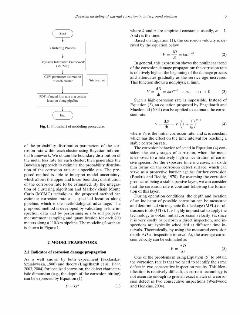
As shown in Figure 3, using data extracted from in-direct and direct inspection data for a 110-km pipeline,we chose three candidate distributions to fit the data.The fitting result also shows that GEV is the bestdistribution to describe the uncertainty feature of themetal loss rate with the lowest Kolmogorov–Smirnovstatistic.
At the most extreme level of the GEV distribution,data are scarce, where for design and maintenance pur-poses, we are interested in the extreme level (tail behav-ior). Because of the scarce observation of extreme metalloss rate, it is difficult to use the limited data within eachcluster to form a relatively accurate empirical PDF ofthe metal loss rate, especially to build up a PDF with anexact tail behavior. Therefore, we have to develop an in-ferential process to maximize the use of available data.Bayesian inferential framework is suitable as a basis toundertake the extreme value analysis (Coles and Tawn,1996).
Within each cluster, the metal loss rate has a GEVdistribution:
r ∼ GEV(μ,σ ,ξ) (11)
where r is metal loss rate, and μ, σ , and ξ are the lo-cation, scale, and shape parameter, respectively. Let usconsider that each observation of metal loss rate is in-dependent from others. The likelihood function is
L(μ, σ, ξ |r) = 1σ n
exp
{−
n∑i=1
[1+ ξ
ri − μ
σ
]−1/ξ}
n∏i=1
[1+ ξ
ri − μ
σ
]−1/ξ−1 (12)
where r = (r1, r2, r3, ..., rn), 1+ ξ( r−μ
σ) > 0, and n is the
number of observations.Notice that for σ > 0, the parameterization φ = ln(σ )
is easier to work with, since σ is constrained to bepositive. Thus, if we substitute σ = exp(φ) into Equa-tion (12), then multiply Jacobian, we can get the expres-sion of likelihood function in terms of μ, φ, ξ .
L(μ, φ, ξ |r) = exp
{(1− n)φ −
n∑i=1
[1+ ξ
ri − μ
exp(φ)
]−1/ξ}
n∏i=1
[1+ ξ
ri − μ
exp(φ)
]−1/ξ−1
(13)

6 Wang, Yajima, Liang & Castaneda
0.01 0.02 0.03 0.04 0.05 0.06 0.07 0.08
0.01
0.25 0.5 0.75 0.9 0.95
0.99 0.995
0.999 0.9995
0.9999
Metal Loss Rate (mm/year)
Pro
babi
lity
Metal Loss Rate
GEV (K-S Dn=0.17)
Lognormal (K-S Dn=0.19)
Gamma (K-S Dn=0.21)
Fig. 3. Probability plot of metal loss rate based on data obtained from direct inspection along the 110-km pipeline. TheKolmogorov–Smirnov (K–S) test was performed, and Dn is the K–S statistic.
If we consider that no prior information is avail-able about the parameters of the GEV distribution (al-though we have the observation of metal loss rate, westill do not have enough prior information about the dis-tribution of μ, φ, ξ), a normal assumption is introducedto build up the prior distribution of GEV parameters.
π(μ, φ, ξ) = π(μ) · π(φ) · π(ξ) (14)
where μ ∼ N(0,σμ), φ ∼ N(0,σφ), ξ ∼ N(0,σξ ). We useπ(.) to denote prior distribution and π*(.) to denoteposterior distribution hereafter.
To make the prior distribution almost flat, we havearbitrarily chosen a large variance, since we do nothave enough information regarding the prior parameterdistribution. According the Bayesian inferential frame-work,
π∗(μ, φ, ξ) = π(μ, φ, ξ)L(μ, φ, ξ |r)∫π(μ, φ, ξ)L(μ, φ, ξ |r)dμdφdξ
(15)
Because there are three parameters in the GEV dis-tribution, we need a sampling process that can generatesamples from a multivariate distribution. We set a com-bination of Gibbs sampling (Ching et al., 2006) and theMetropolis–Hastings (M–H) algorithm. The key to theGibbs sampler is that we only consider univariate con-ditional distributions Equation (18). Such conditionaldistributions are practicable in simulation since there isno analytical conjugate posterior distribution for nor-mal prior distribution which is updated by GEV like-lihood function. The scheme comes from work by Ge-man and Geman (1984), Metropolis et al. (1953), andHastings (1970).
According to Equation (15), the posterior densityfunction can be written in the form:
π∗(μ, φ, ξ) ∝ π(μ, φ, ξ)L(μ, φ, ξ |r) (16)
With the prior parameter distribution given in Equa-tion (14),
π(μ, φ, ξ)L(μ, φ, ξ |r) = π(μ)π(φ)π(ξ)L(μ, φ, ξ |r)
(17)
we can form the full conditional functions for Gibbssampling:⎧⎪⎪⎪⎪⎨
⎪⎪⎪⎪⎩
π(μ∗|φ, ξ) = π(μ)L(μ, φ, ξ |r)
π(φ∗|μ∗, ξ) = π(φ)L(μ∗, φ, ξ |r)
π(ξ ∗|μ∗, φ∗) = π(ξ)L(μ∗, φ∗, ξ |r)
(18)
where μ*, φ*, and ξ* are new candidates of GEV pa-rameters for sampling. To process the M–H algorithm, aproposal distribution is needed to draw μ*, φ*, ξ* giventhe current state. This proposal distribution and its pa-rameters may have a strong influence on the robustnessof the simulation process (Dai et al., 2012). In this work,three Gaussian proposal functions are chosen, as shownbelow:
μ∗ = μ+ ωμ; φ∗ = φ + ωφ ; ξ ∗ = ξ + ωξ
where ωμ, ωφ , and ωξ are normally distributed with zeromeans and a certain standard deviation (STD) that wecall jump length. The proposal distributions determinethe correlation between two successive statuses withinthe Markov chain. Here, the jump length is chosen care-fully so that the acceptance probability will be in theapproximate range of 40% to 60%. This is because a

Bayesian modeling of external corrosion in underground pipelines 7
reasonable acceptance probability will make the M–Halgorithm avoid the local optimization problem, and thesuitable acceptance probability will guarantee the gen-erated samples from Gibbs sampling process representthe posterior distributions (Zhang et al., 2013).
By employing the M–H algorithm within each cluster,the realizations of the GEV parameters were used toestimate the posterior distributions of μ, φ, ξ by usingthe maximum likelihood estimation.
Since the uncertainty of distribution parameters istaken into consideration, the model uncertainty can bereflected by estimating the upper and lower bound (i.e.,the 95% credibility interval) of the PDF for the param-eters (μ, φ, ξ). Then, we develop the upper and lowerbound distribution of metal loss rate by plugging theboundary values of the parameters (μ, φ, ξ) into the dis-tribution function for the metal loss rate.
The distributions of metal loss rate are descriptionsof the random property at an average level withineach cluster. However, we are more interested in thedistribution at a specific location where the corro-sion event occurs. Since we developed the distribu-tions within the clusters, we have some prior informa-tion regarding the metal loss rate at a certain point,although at an average level. In addition, we alsohave the feature vector (location and soil properties),which allows the Bayesian inferential framework to beused for estimating the distribution of the metal lossrate.
In order to estimate the distribution of the metal lossrate at a specific location, we must first build up a train-ing matrix using soil measurement data to evaluate thelikelihood function value. In the training matrix [X,R],each row represents all the features of one defect pointXi and the corresponding metal loss rate Ri. The criticalparameters for corrosion soils are included
Xi = [CP, Eh, Resistivity, pH, [CO2−3 ], [HCO
−3 ], [Cl−],
[SO2−4 ], Soil Moisture]
where CP is the distance from the nearest cathodic pro-tection station to the defect, Eh is the half-cell potential,[.] is the concentration for each ionic species, and pH in-dicates the activity of H+ ions.
A multivariable normal assumption is introduced toform the joint distribution of all the features and metalloss rate. The likelihood function is given by:
L(r |x) = f ([x,r ])P(r)
(19)
where x is the feature vector of a certain location, r is thecorresponding metal loss rate, and P(r) is the marginal
probability distribution of metal loss rate.
f ([x,r ]) = 1
(2π)5 |�|1/2
× exp(−12
([x,r ]− μ)T �−1([x,r ]− μ)) (20)
where � is the covariance matrix of [X,R], and ❘� ❘ is thedeterminant of �. The distribution of metal loss rate ineach cluster can be the prior distribution. Therefore, theupdated expression is
π∗(r) ∝ π(r)L(r |x) (21)
where π*(r) is posterior and π(r) is prior.Using the M–H algorithm to estimate the posterior,
an updated distribution can be formed from the MCMCsampling process.
The complete algorithm of the proposed methodol-ogy is shown in Appendix B.
3 MODEL APPLICATIONS
The proposed model is applied to predict the externalcorrosion of a pipeline section that is 110 km in lengthused for transmission of oil product go downstream op-erations. The diameter of the pipeline is 457.2 mm andthe wall thickness varies between the sections along thelength of the pipeline, with wall thicknesses of 6.4, 9.5,10.3, and 12.7 mm. According to the database for thepipeline section, measurements from in-line inspectionsperformed in 2005, 2010, and 2011 are available. The2005 and 2010 inspections contain information aboutdefects along the entire length of the pipeline; however,the 2011 inspection was only performed on a portionof the pipeline. The operation times of the sections ofpipeline also vary, with most sections having been in ser-vice for more than 29 years. In this analysis, we use theresults obtained in the 2010 in-line inspection, the mostrecent inspection that includes data from the full lengthof the pipeline. During the 2010 pipeline inspection, atotal of 1,924 external events related to wall thicknessmetal loss were detected.
3.1 Clustering results
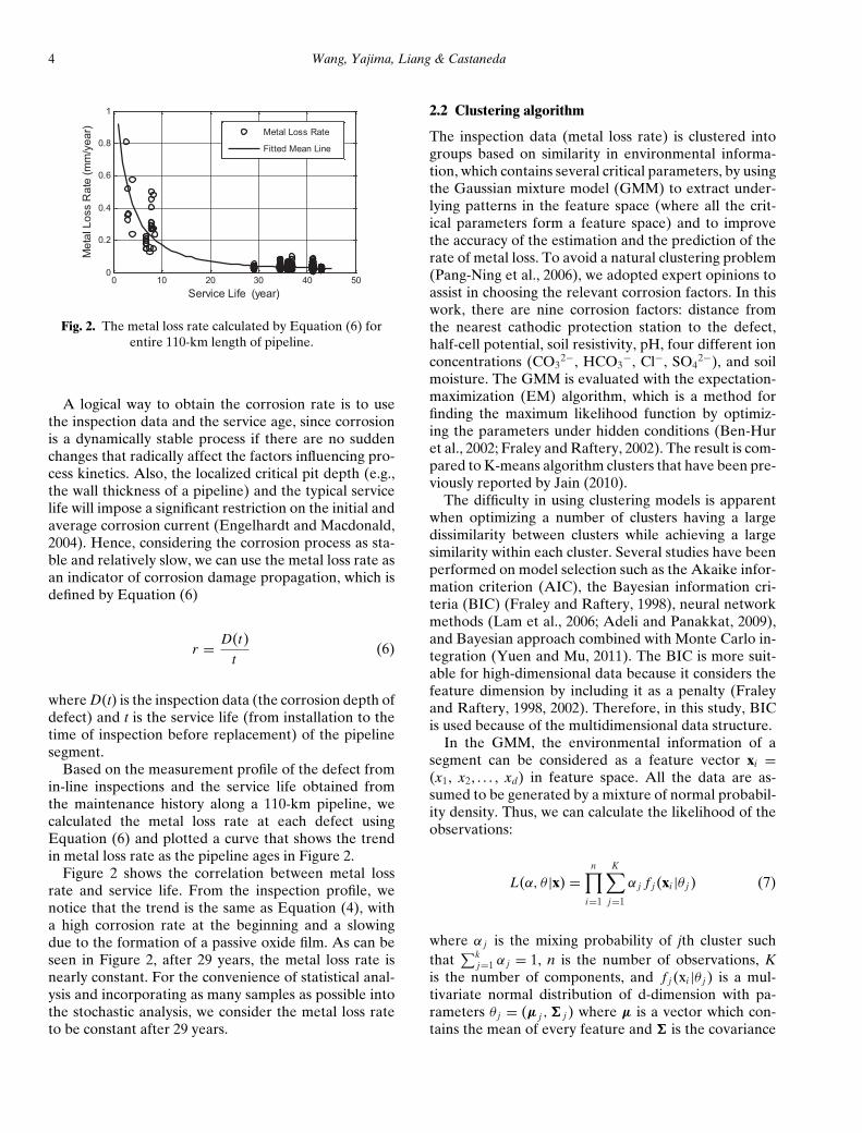
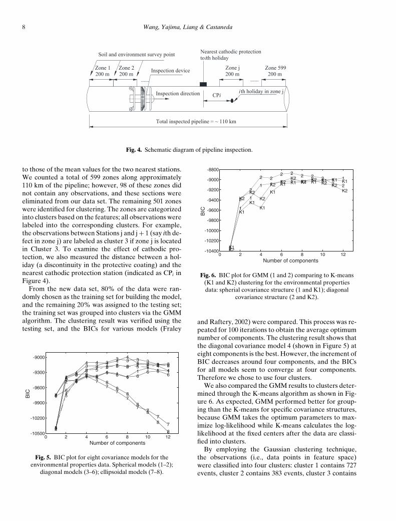
Prior to clustering, it was necessary to create a new dataset based on the physical distance along the pipeline,since the environmental and soil condition measure-ments were collected every 200 m during the site mea-surement. Locations where measurements were takenare referred to as “stations” and the section of pipelinebetween two stations is called a “zone.” The physicalproperties of a given zone are considered to be similar
8 Wang, Yajima, Liang & Castaneda
Zone 1200 m
Zone 2200 m
Zone j200 m
Zone 599200 m
...... ......Inspection device
Inspection direction
Nearest cathodic protectionto ith holidaySoil and environment survey point
CPiith holiday in zone j
Total inspected pipeline = ~ 110 km
Fig. 4. Schematic diagram of pipeline inspection.
to those of the mean values for the two nearest stations.We counted a total of 599 zones along approximately110 km of the pipeline; however, 98 of these zones didnot contain any observations, and these sections wereeliminated from our data set. The remaining 501 zoneswere identified for clustering. The zones are categorizedinto clusters based on the features; all observations werelabeled into the corresponding clusters. For example,the observations between Stations j and j+ 1 (say ith de-fect in zone j) are labeled as cluster 3 if zone j is locatedin Cluster 3. To examine the effect of cathodic pro-tection, we also measured the distance between a hol-iday (a discontinuity in the protective coating) and thenearest cathodic protection station (indicated as CPi inFigure 4).
From the new data set, 80% of the data were ran-domly chosen as the training set for building the model,and the remaining 20% was assigned to the testing set;the training set was grouped into clusters via the GMMalgorithm. The clustering result was verified using thetesting set, and the BICs for various models (Fraley
0 2 4 6 8 10 12-10500
-10200
-9900
-9600
-9300
-9000
1
1
11 1
1 11
11 1 1
Number of components
BIC
2
2 2
2 2 2 2 2 2 2 2 2
3
33
3 33
3 3 3 33 3
4
44
4 4 4 44
4 4 44
5
5
5
5 55 5 5 5 5 5 5
66
66 6
6 6 6 66 6
6
7
7 77
77
7
7
77
7
7
8
88 8
88
88
8
8
8
8
Fig. 5. BIC plot for eight covariance models for theenvironmental properties data. Spherical models (1–2);
diagonal models (3–6); ellipsoidal models (7–8).
0 2 4 6 8 10 12-10400
-10200
-10000
-9800
-9600
-9400
-9200
-9000
-8800
1
1
1
1 1 1 1 1 1 1 1 1
Number of components
BIC
2
2
2
2 22 2 2 2 2
2 2
K1
K1
K1K1
K1
K1 K1 K1 K1 K1 K1 K1
K2
K2K2
K2
K2K2
K2K2 K2
K2 K2K2
Fig. 6. BIC plot for GMM (1 and 2) comparing to K-means(K1 and K2) clustering for the environmental propertiesdata: spherial covariance structure (1 and K1); diagonal
covariance structure (2 and K2).
and Raftery, 2002) were compared. This process was re-peated for 100 iterations to obtain the average optimumnumber of components. The clustering result shows thatthe diagonal covariance model 4 (shown in Figure 5) ateight components is the best. However, the increment ofBIC decreases around four components, and the BICsfor all models seem to converge at four components.Therefore we chose to use four clusters.
We also compared the GMM results to clusters deter-mined through the K-means algorithm as shown in Fig-ure 6. As expected, GMM performed better for group-ing than the K-means for specific covariance structures,because GMM takes the optimum parameters to max-imize log-likelihood while K-means calculates the log-likelihood at the fixed centers after the data are classi-fied into clusters.
By employing the Gaussian clustering technique,the observations (i.e., data points in feature space)were classified into four clusters: cluster 1 contains 727events, cluster 2 contains 383 events, cluster 3 contains
Bayesian modeling of external corrosion in underground pipelines 9
-400-200
0E
h
0
5
10
pH
0
5
10
[Cl- ]
0
2
x 105
Res
istiv
ityC
1C
2C
3C
4
0 200 400 600 800 1000 1200 1400Defect ID
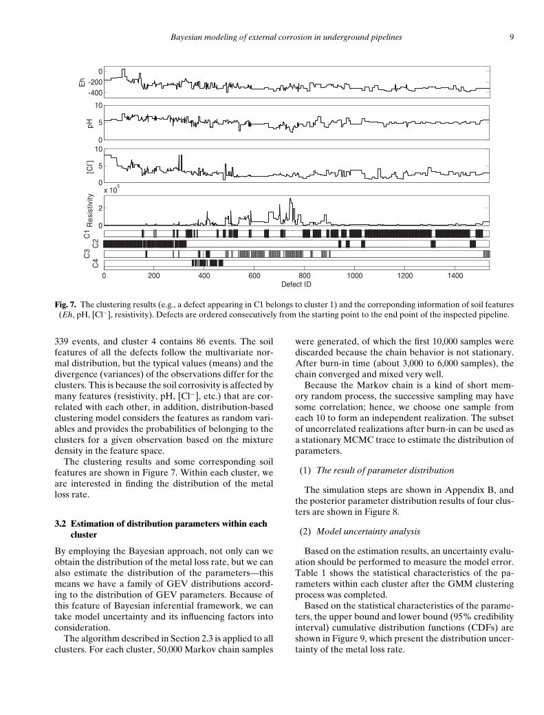
Fig. 7. The clustering results (e.g., a defect appearing in C1 belongs to cluster 1) and the correponding information of soil features(Eh, pH, [Cl−], resistivity). Defects are ordered consecutively from the starting point to the end point of the inspected pipeline.
339 events, and cluster 4 contains 86 events. The soilfeatures of all the defects follow the multivariate nor-mal distribution, but the typical values (means) and thedivergence (variances) of the observations differ for theclusters. This is because the soil corrosivity is affected bymany features (resistivity, pH, [Cl−], etc.) that are cor-related with each other, in addition, distribution-basedclustering model considers the features as random vari-ables and provides the probabilities of belonging to theclusters for a given observation based on the mixturedensity in the feature space.
The clustering results and some corresponding soilfeatures are shown in Figure 7. Within each cluster, weare interested in finding the distribution of the metalloss rate.
3.2 Estimation of distribution parameters within eachcluster
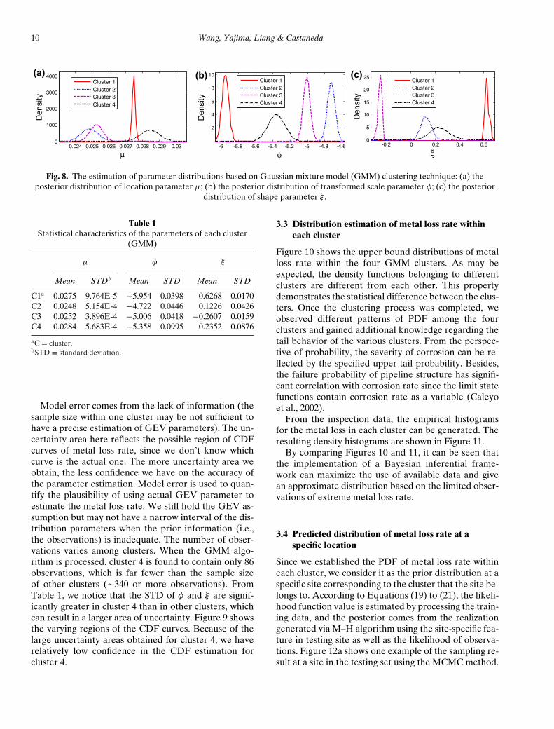
By employing the Bayesian approach, not only can weobtain the distribution of the metal loss rate, but we canalso estimate the distribution of the parameters—thismeans we have a family of GEV distributions accord-ing to the distribution of GEV parameters. Because ofthis feature of Bayesian inferential framework, we cantake model uncertainty and its influencing factors intoconsideration.
The algorithm described in Section 2.3 is applied to allclusters. For each cluster, 50,000 Markov chain samples
were generated, of which the first 10,000 samples werediscarded because the chain behavior is not stationary.After burn-in time (about 3,000 to 6,000 samples), thechain converged and mixed very well.
Because the Markov chain is a kind of short mem-ory random process, the successive sampling may havesome correlation; hence, we choose one sample fromeach 10 to form an independent realization. The subsetof uncorrelated realizations after burn-in can be used asa stationary MCMC trace to estimate the distribution ofparameters.
(1) The result of parameter distribution
The simulation steps are shown in Appendix B, andthe posterior parameter distribution results of four clus-ters are shown in Figure 8.
(2) Model uncertainty analysis
Based on the estimation results, an uncertainty evalu-ation should be performed to measure the model error.Table 1 shows the statistical characteristics of the pa-rameters within each cluster after the GMM clusteringprocess was completed.
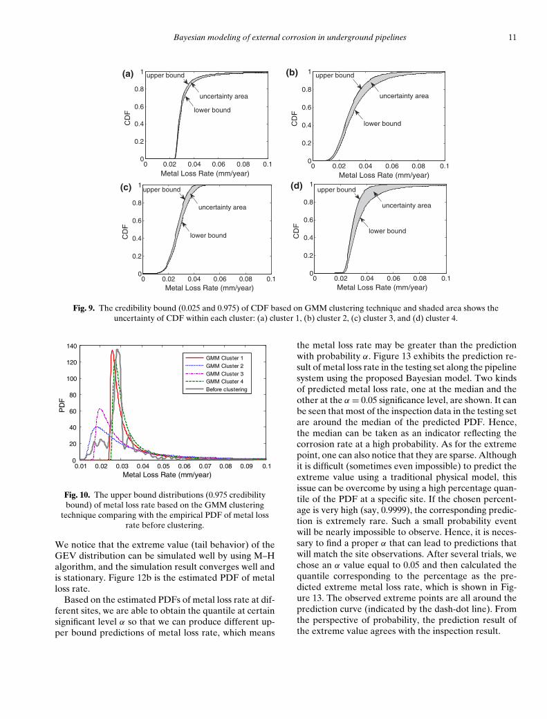
Based on the statistical characteristics of the parame-ters, the upper bound and lower bound (95% credibilityinterval) cumulative distribution functions (CDFs) areshown in Figure 9, which present the distribution uncer-tainty of the metal loss rate.
10 Wang, Yajima, Liang & Castaneda
0.024 0.025 0.026 0.027 0.028 0.029 0.030
1000
μ
2000
3000
4000
Den
sity
Cluster 1Cluster 2Cluster 3Cluster 4
(a)
-6 -5.8 -5.6 -5.4 -5.2 -5 -4.8 -4.6
2
4
6
8
10
φ
Den
sity
Cluster 1Cluster 2Cluster 3Cluster 4
(b)
-0.2 0 0.2 0.4 0.60
5
10
15
20
25
ξ
Den
sity
Cluster 1Cluster 2Cluster 3Cluster 4
(c)
Fig. 8. The estimation of parameter distributions based on Gaussian mixture model (GMM) clustering technique: (a) theposterior distribution of location parameter μ; (b) the posterior distribution of transformed scale parameter φ; (c) the posterior
distribution of shape parameter ξ .
Table 1Statistical characteristics of the parameters of each cluster
(GMM)
μ φ ξ
Mean STDb Mean STD Mean STD
C1a 0.0275 9.764E-5 −5.954 0.0398 0.6268 0.0170C2 0.0248 5.154E-4 −4.722 0.0446 0.1226 0.0426C3 0.0252 3.896E-4 −5.006 0.0418 −0.2607 0.0159C4 0.0284 5.683E-4 −5.358 0.0995 0.2352 0.0876
aC = cluster.bSTD = standard deviation.
Model error comes from the lack of information (thesample size within one cluster may be not sufficient tohave a precise estimation of GEV parameters). The un-certainty area here reflects the possible region of CDFcurves of metal loss rate, since we don’t know whichcurve is the actual one. The more uncertainty area weobtain, the less confidence we have on the accuracy ofthe parameter estimation. Model error is used to quan-tify the plausibility of using actual GEV parameter toestimate the metal loss rate. We still hold the GEV as-sumption but may not have a narrow interval of the dis-tribution parameters when the prior information (i.e.,the observations) is inadequate. The number of obser-vations varies among clusters. When the GMM algo-rithm is processed, cluster 4 is found to contain only 86observations, which is far fewer than the sample sizeof other clusters (�340 or more observations). FromTable 1, we notice that the STD of φ and ξ are signif-icantly greater in cluster 4 than in other clusters, whichcan result in a larger area of uncertainty. Figure 9 showsthe varying regions of the CDF curves. Because of thelarge uncertainty areas obtained for cluster 4, we haverelatively low confidence in the CDF estimation forcluster 4.
3.3 Distribution estimation of metal loss rate withineach cluster
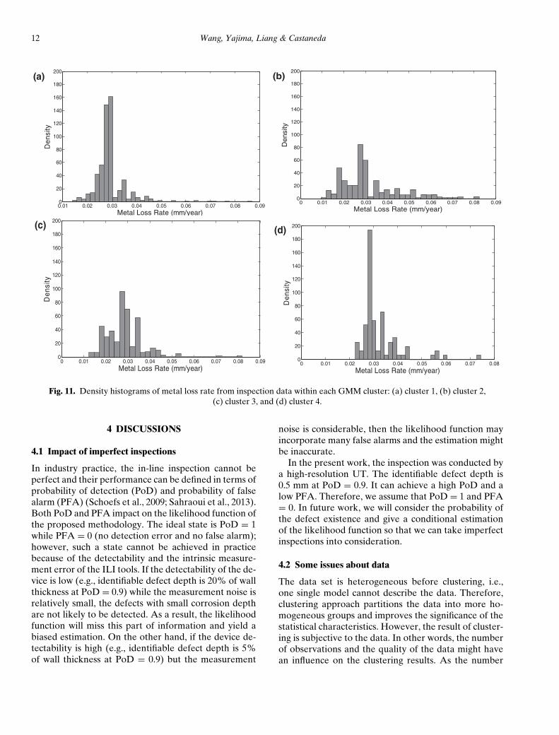
Figure 10 shows the upper bound distributions of metalloss rate within the four GMM clusters. As may beexpected, the density functions belonging to differentclusters are different from each other. This propertydemonstrates the statistical difference between the clus-ters. Once the clustering process was completed, weobserved different patterns of PDF among the fourclusters and gained additional knowledge regarding thetail behavior of the various clusters. From the perspec-tive of probability, the severity of corrosion can be re-flected by the specified upper tail probability. Besides,the failure probability of pipeline structure has signifi-cant correlation with corrosion rate since the limit statefunctions contain corrosion rate as a variable (Caleyoet al., 2002).
From the inspection data, the empirical histogramsfor the metal loss in each cluster can be generated. Theresulting density histograms are shown in Figure 11.
By comparing Figures 10 and 11, it can be seen thatthe implementation of a Bayesian inferential frame-work can maximize the use of available data and givean approximate distribution based on the limited obser-vations of extreme metal loss rate.
3.4 Predicted distribution of metal loss rate at aspecific location
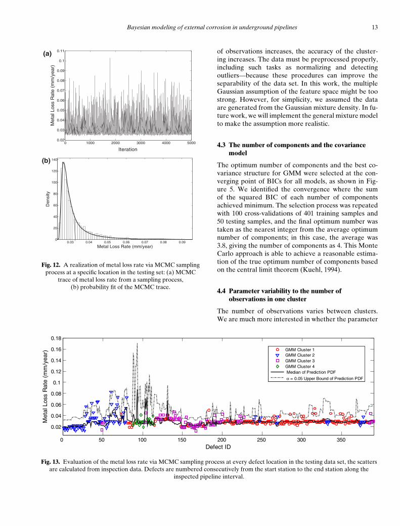
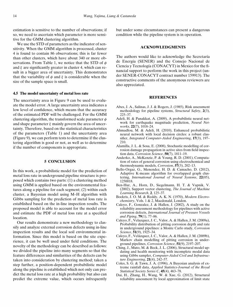
Since we established the PDF of metal loss rate withineach cluster, we consider it as the prior distribution at aspecific site corresponding to the cluster that the site be-longs to. According to Equations (19) to (21), the likeli-hood function value is estimated by processing the train-ing data, and the posterior comes from the realizationgenerated via M–H algorithm using the site-specific fea-ture in testing site as well as the likelihood of observa-tions. Figure 12a shows one example of the sampling re-sult at a site in the testing set using the MCMC method.
Bayesian modeling of external corrosion in underground pipelines 11
0 0.02 0.04 0.06 0.08 0.10
0.2
0.4
0.6
0.8
1
Metal Loss Rate (mm/year)
CD
F
upper bound
lower bound
uncertainty area
(a)
0 0.02 0.04 0.06 0.08 0.10
0.2
0.4
0.6
0.8
1
Metal Loss Rate (mm/year)
CD
F
upper bound
lower bound
(b)
uncertainty area
0 0.02 0.04 0.06 0.08 0.10
0.2
0.4
0.6
0.8
1
Metal Loss Rate (mm/year)
CD
F
(c) upper bound
lower bound
uncertainty area
0 0.02 0.04 0.06 0.08 0.10
0.2
0.4
0.6
0.8
1
Metal Loss Rate (mm/year)C
DF
upper bound
lower bound
uncertainty area
(d)
Fig. 9. The credibility bound (0.025 and 0.975) of CDF based on GMM clustering technique and shaded area shows theuncertainty of CDF within each cluster: (a) cluster 1, (b) cluster 2, (c) cluster 3, and (d) cluster 4.
0.01 0.02 0.03 0.04 0.05 0.06 0.07 0.08 0.09 0.10
20
40
60
80
100
120
140
Metal Loss Rate (mm/year)
PD
F
GMM Cluster 1GMM Cluster 2GMM Cluster 3GMM Cluater 4Before clustering
Fig. 10. The upper bound distributions (0.975 credibilitybound) of metal loss rate based on the GMM clustering
technique comparing with the empirical PDF of metal lossrate before clustering.
We notice that the extreme value (tail behavior) of theGEV distribution can be simulated well by using M–Halgorithm, and the simulation result converges well andis stationary. Figure 12b is the estimated PDF of metalloss rate.
Based on the estimated PDFs of metal loss rate at dif-ferent sites, we are able to obtain the quantile at certainsignificant level α so that we can produce different up-per bound predictions of metal loss rate, which means
the metal loss rate may be greater than the predictionwith probability α. Figure 13 exhibits the prediction re-sult of metal loss rate in the testing set along the pipelinesystem using the proposed Bayesian model. Two kindsof predicted metal loss rate, one at the median and theother at the α = 0.05 significance level, are shown. It canbe seen that most of the inspection data in the testing setare around the median of the predicted PDF. Hence,the median can be taken as an indicator reflecting thecorrosion rate at a high probability. As for the extremepoint, one can also notice that they are sparse. Althoughit is difficult (sometimes even impossible) to predict theextreme value using a traditional physical model, thisissue can be overcome by using a high percentage quan-tile of the PDF at a specific site. If the chosen percent-age is very high (say, 0.9999), the corresponding predic-tion is extremely rare. Such a small probability eventwill be nearly impossible to observe. Hence, it is neces-sary to find a proper α that can lead to predictions thatwill match the site observations. After several trials, wechose an α value equal to 0.05 and then calculated thequantile corresponding to the percentage as the pre-dicted extreme metal loss rate, which is shown in Fig-ure 13. The observed extreme points are all around theprediction curve (indicated by the dash-dot line). Fromthe perspective of probability, the prediction result ofthe extreme value agrees with the inspection result.
12 Wang, Yajima, Liang & Castaneda
0.01 0.02 0.03 0.04 0.05 0.06 0.07 0.08 0.090
20
40
60
80
100
120
140
160
180
200
Metal Loss Rate (mm/year)
Den
sity
(a)
0 0.01 0.02 0.03 0.04 0.05 0.06 0.07 0.08 0.090
20
40
60
80
100
120
140
160
180
200
Metal Loss Rate (mm/year)
Den
sity
(b)
0 0.01 0.02 0.03 0.04 0.05 0.06 0.07 0.08 0.090
20
40
60
80
100
120
140
160
180
200
Metal Loss Rate (mm/year)
Den
sity
(c)
0 0.01 0.02 0.03 0.04 0.05 0.06 0.07 0.080
20
40
60
80
100
120
140
160
180
200
Metal Loss Rate (mm/year)
Den
sity
(d)
Fig. 11. Density histograms of metal loss rate from inspection data within each GMM cluster: (a) cluster 1, (b) cluster 2,(c) cluster 3, and (d) cluster 4.
4 DISCUSSIONS
4.1 Impact of imperfect inspections
In industry practice, the in-line inspection cannot beperfect and their performance can be defined in terms ofprobability of detection (PoD) and probability of falsealarm (PFA) (Schoefs et al., 2009; Sahraoui et al., 2013).Both PoD and PFA impact on the likelihood function ofthe proposed methodology. The ideal state is PoD = 1while PFA = 0 (no detection error and no false alarm);however, such a state cannot be achieved in practicebecause of the detectability and the intrinsic measure-ment error of the ILI tools. If the detectability of the de-vice is low (e.g., identifiable defect depth is 20% of wallthickness at PoD = 0.9) while the measurement noise isrelatively small, the defects with small corrosion depthare not likely to be detected. As a result, the likelihoodfunction will miss this part of information and yield abiased estimation. On the other hand, if the device de-tectability is high (e.g., identifiable defect depth is 5%of wall thickness at PoD = 0.9) but the measurement
noise is considerable, then the likelihood function mayincorporate many false alarms and the estimation mightbe inaccurate.
In the present work, the inspection was conducted bya high-resolution UT. The identifiable defect depth is0.5 mm at PoD = 0.9. It can achieve a high PoD and alow PFA. Therefore, we assume that PoD = 1 and PFA= 0. In future work, we will consider the probability ofthe defect existence and give a conditional estimationof the likelihood function so that we can take imperfectinspections into consideration.
4.2 Some issues about data
The data set is heterogeneous before clustering, i.e.,one single model cannot describe the data. Therefore,clustering approach partitions the data into more ho-mogeneous groups and improves the significance of thestatistical characteristics. However, the result of cluster-ing is subjective to the data. In other words, the numberof observations and the quality of the data might havean influence on the clustering results. As the number
Bayesian modeling of external corrosion in underground pipelines 13
0 1000 2000 3000 4000 50000.02
0.03
0.04
0.05
0.06
0.07
0.08
0.09
0.1
0.11
Iteration
Met
al L
oss
Rat
e (m
m/y
ear)
(a)
0.03 0.04 0.05 0.06 0.07 0.08 0.090
20
40
60
80
100
120
140
Metal Loss Rate (mm/year)
Den
sity
(b)
Fig. 12. A realization of metal loss rate via MCMC samplingprocess at a specific location in the testing set: (a) MCMC
trace of metal loss rate from a sampling process,(b) probability fit of the MCMC trace.
of observations increases, the accuracy of the cluster-ing increases. The data must be preprocessed properly,including such tasks as normalizing and detectingoutliers—because these procedures can improve theseparability of the data set. In this work, the multipleGaussian assumption of the feature space might be toostrong. However, for simplicity, we assumed the dataare generated from the Gaussian mixture density. In fu-ture work, we will implement the general mixture modelto make the assumption more realistic.
4.3 The number of components and the covariancemodel
The optimum number of components and the best co-variance structure for GMM were selected at the con-verging point of BICs for all models, as shown in Fig-ure 5. We identified the convergence where the sumof the squared BIC of each number of componentsachieved minimum. The selection process was repeatedwith 100 cross-validations of 401 training samples and50 testing samples, and the final optimum number wastaken as the nearest integer from the average optimumnumber of components; in this case, the average was3.8, giving the number of components as 4. This MonteCarlo approach is able to achieve a reasonable estima-tion of the true optimum number of components basedon the central limit theorem (Kuehl, 1994).
4.4 Parameter variability to the number ofobservations in one cluster
The number of observations varies between clusters.We are much more interested in whether the parameter
0 50 100 150 200 250 300 350
0.02
0.04
0.06
0.08
0.1
0.12
0.14
0.16
0.18
Defect ID
Met
al L
oss
Rat
e (m
m/y
ear)
GMM Cluster 1GMM Cluster 2GMM Cluster 3GMM Cluster 4 Median of Prediction PDF α = 0.05 Upper Bound of Prediction PDF
Fig. 13. Evaluation of the metal loss rate via MCMC sampling process at every defect location in the testing data set, the scattersare calculated from inspection data. Defects are numbered consecutively from the start station to the end station along the
inspected pipeline interval.
14 Wang, Yajima, Liang & Castaneda
estimation is sensitive to the number of observations; ifso, we need to ascertain which parameter is more sensi-tive for the GMM clustering algorithm.
We use the STD of parameters as the indicator of sen-sitivity. When the GMM algorithm is processed, cluster4 is found to contain 86 observations; this is far fewerthan other clusters, which have about 340 or more ob-servations. From Table 1, we notice that the STD of φ
and ξ are significantly greater in cluster 4, which can re-sult in a bigger area of uncertainty. This demonstratesthat the variability of φ and ξ is considerable when thesize of the sample space is small.
4.5 The model uncertainty of metal loss rate
The uncertainty area in Figure 9 can be used to evalu-ate the model error. A large uncertainty area indicates alow level of confidence, which means that the accuracyof the estimated PDF will be challenged. For the GMMclustering algorithm, the transformed scale parameter φ
and shape parameter ξ mainly govern the area of uncer-tainty. Therefore, based on the statistical characteristicsof the parameters (Table 1) and the uncertainty area(Figure 9), we can perform tests to determine if the clus-tering algorithm is good or not, as well as to determineif the number of components is appropriate.
5 CONCLUSION
In this work, a probabilistic model for the prediction ofmetal loss rate in underground pipeline structure is pro-posed which contains two parts: (1) a clustering methodusing GMM is applied based on the environmental fea-tures along a pipeline for each segment; (2) within eachcluster, a Bayesian model using M–H algorithm withGibbs sampling for the prediction of metal loss rate isestablished based on the in-line inspection results. Theproposed model is able to account for the model errorand estimate the PDF of metal loss rate at a specifiedlocation.
Our results demonstrate a new methodology to clas-sify and analyze external corrosion defects using in-lineinspection results and the local soil environmental in-formation. Since this model is based on the site expe-rience, it can be well used under field conditions. Thenovelty of the methodology can be described as follows:we divided the pipeline into many segments so that thefeature differences and similarities of the defects can betaken into consideration by clustering method; taken astep further, a position-dependent probabilistic modelalong the pipeline is established which not only can pre-dict the metal loss rate at a high probability but also canpredict the extreme value, which occurs infrequently
but under some circumstances can present a dangerouscondition while the pipeline system is in operation.
ACKNOWLEDGMENTS
The authors would like to acknowledge the Secretarıade Energıa (SENER) and the Consejo Nacional deCiencia y Tecnologıa (CONACYT) in Mexico for the fi-nancial support to perform the work in this project (un-der SENER-CONACYT contract number 159913). Theconstructive comments of the anonymous reviewers arealso appreciated.
REFERENCES
Abes, J. A., Salinas, J. J. & Rogers, J. (1985), Risk assessmentmethodology for pipeline systems, Structural Safety, 2(3),225–37.
Adeli, H. & Panakkat, A. (2009), A probabilistic neural net-work for earthquake magnitude prediction, Neural Net-works, 22(7), 1018–24.
Ahmadlou, M. & Adeli, H. (2010), Enhanced probabilisticneural network with local decision circles: a robust clas-sifier, Integrated Computer-Aided Engineering, 17(3), 197–210.
Alamilla, J. L. & Sosa, E. (2008), Stochastic modelling of cor-rosion damage propagation in active sites from field inspec-tion data, Corrosion Science, 50(7), 1811–19.
Anderko, A., McKenzie, P. & Young, R. D. (2001), Computa-tion of rates of general corrosion using electrochemical andthermodynamic models, Corrosion, 57(3), 202–13.
Bello-Orgaz, G., Menendez, H. D. & Camacho, D. (2012),Adaptive K-means algorithm for overlapped graph clus-tering, International Journal of Neural Systems, 22(05),1250018.
Ben-Hur, A., Horn, D., Siegelmann, H. T. & Vapnik, V.(2002), Support vector clustering, The Journal of MachineLearning Research, 2, 125–37.
Bockris, J. O. M. & Reddy, A. K. N. (1970), Modern Electro-chemistry, Vols. 1 & 2, Macdonald, London.
Caleyo, F., Gonzalez, J. & Hallen, J. (2002), A study on thereliability assessment methodology for pipelines with activecorrosion defects, International Journal of Pressure Vesselsand Piping, 79(1), 77–86.
Caleyo, F., Velazquez, J. C., Valor, A. & Hallen, J. M. (2009a),Probability distribution of pitting corrosion depth and ratein underground pipelines: a Monte Carlo study, CorrosionScience, 51(9), 1925–34.
Caleyo, F., Velazquez, J. C., Valor, A. & Hallen, J. M. (2009b),Markov chain modelling of pitting corrosion in under-ground pipelines, Corrosion Science, 51(9), 2197–207.
Ching, J., Muto, M. & Beck, J. L. (2006), Structural model up-dating and health monitoring with incomplete modal datausing Gibbs sampler, Computer-Aided Civil and Infrastruc-ture Engineering, 21(4), 242–57.
Coles, S. G. & Tawn, J. A. (1996), A Bayesian analysis of ex-treme rainfall data, Applied Statistics-Journal of the RoyalStatistical Society Series C, 45(4), 463–78.
Dai, H., Zhang, H., Wang, W. & Xue, G. (2012), Structuralreliability assessment by local approximation of limit state
Bayesian modeling of external corrosion in underground pipelines 15
functions using adaptive Markov chain simulation and sup-port vector regression, Computer-Aided Civil and Infras-tructure Engineering, 27(9), 676–86.
DeWaard, C. & Milliams, D. (1975), Carbonic acid corrosionof steel, Corrosion, 31(5), 177–81.
Engelhardt, G., Macdonald, D. & Urquidi-Macdonald, M.(1999), Development of fast algorithms for estimating stresscorrosion crack growth rate, Corrosion Science, 41(12),2267–302.
Engelhardt, G. & Macdonald, D. D. (2004), Unification of thedeterministic and statistical approaches for predicting lo-calized corrosion damage. I. Theoretical foundation, Cor-rosion Science, 46(11), 2755–80.
Fraley, C. & Raftery, A. E. (1998), How many clusters? Whichclustering method? Answers via model-based cluster anal-ysis, The Computer Journal, 41(8), 578–88.
Fraley, C. & Raftery, A. E. (2002), Model-based clustering,discriminant analysis, and density estimation, Journal of theAmerican Statistical Association, 97(458), 611–31.
Fraley, C. & Raftery, A. E. (2007), Bayesian regularizationfor normal mixture estimation and model-based clustering,Journal of Classification, 24(2), 155–81.
Fraley, C., Raftery, A. E., Murphy, T. B. & Scrucca, L. (2012),MCLUST Version 4 for R: Normal Mixture Modeling forModel-Based Clustering, Classification, and Density Estima-tion, Technical Report no. 597, Department of Statistics,University of Washington, June 2012.
Geman, S. & Geman, D. (1984), Stochastic relaxation, Gibbsdistributions, and the Bayesian restoration of images, IEEETransactions on Pattern Analysis and Machine Intelligence,PAMI-6(6), 721–41.
Ghosh-Dastidar, S. & Adeli, H. (2003), Wavelet-clustering-neural network model for freeway incident detection,Computer-Aided Civil and Infrastructure Engineering,18(5), 325–38.
Hastings, W. K. (1970), Monte Carlo sampling methods usingMarkov chains and their applications, Biometrika, 57(1),97–109.
Hong, H. P. (1999), Inspection and maintenance planning ofpipeline under external corrosion considering generation ofnew defects, Structural Safety, 21(3), 203–22.
Jain, A. K. (2010), Data clustering: 50 years beyond K-means,Pattern Recognition Letters, 31(8), 651–66.
Kiefner, J. F. & Kolovich, K. M. (2007), Calculation of a cor-rosion rate using Monte Carlo simulation, CORROSION2007, NACE International, Nashville, TN, March 11–15,2007.
Kodogiannis, V. S., Amina, M. & Petrounias, I. (2013), Aclustering-based fuzzy wavelet neural network model forshort-term load forecasting, International Journal of NeuralSystems, 23(05), 1350024.
Kuehl, R. O. (1994), Statistical Principles of Research Designand Analysis, Duxbury Press, Belmont, CA.
Lam, H. F., Yuen, K. V. & Beck, J. L. (2006), Structural healthmonitoring via measured ritz vectors utilizing artificial neu-ral networks, Computer-Aided Civil and Infrastructure En-gineering, 21(4), 232–41.
Maes, M. A., Faber, M. H. & Dann, M. R. (2009), Hierarchi-cal modeling of pipeline defect growth subject to ILI un-certainty, in Proceedings of the ASME 28th InternationalConference on Ocean, Offshore and Arctic Engineering,ASME, Honolulu, HI, USA, May 31–June 5, 2009.
McLachlan, G. J. & Basford, K. E. (1988), Mixture Models: In-ference and Applications to Clustering, Statistics: Textbooksand Monographs,Vol. 1, Marcel Dekker, New York.
McLachlan, G. J. & Krishnan, T. (2007), The EM Algorithmand Extensions, John Wiley & Sons, New York.
Melchers, R. (2003), Modeling of marine immersion corro-sion for mild and low-alloy steels-part 1: phenomenologicalmodel, Corrosion, 59(4), 319–34.
Melchers, R. (2004), Pitting corrosion of mild steel in marineimmersion environment-part 1: maximum pit depth, Corro-sion, 60(9), 824–36.
Menendez, H. D., Barrero, D. F. & Camacho, D. (2014),A genetic graph-based approach to the partitional clus-tering, International Journal of Neural Systems, 24(03),1430008.
Metropolis, N., Rosenbluth, A. W., Rosenbluth, M. N., Teller,A. H. & Teller, E. (1953), Equation of state calculations byfast computing machines, The Journal of Chemical Physics,21, 1087–92.
Pang-Ning, T., Steinbach, M. & Kumar, V. (2006), Introduc-tion to Data Mining, Addison-Wesley, Boston.
Peabody, A. W., Bianchetti, R. L. & National Associationof Corrosion Engineers (2001), Control of Pipeline Corro-sion, National Association of Corrosion Engineers, Hous-ton, TX.
Peng, F. & Ouyang, Y. (2013), Optimal clustering of railroadtrack maintenance jobs, Computer-Aided Civil and Infras-tructure Engineering, 29(4), 235–47.
Race, J. M., Dawson, S. J., Stanley, L. M. & Kariyawasam,S. (2007), Development of a predictive model for pipelineexternal corrosion rates, Journal of Pipeline Engineering,6(1), 15–29.
Rizzi, M., D’Aloia, M. & Castagnolo, B. (2013), A supervisedmethod for microcalcification cluster diagnosis, IntegratedComputer-Aided Engineering, 20(2), 157–67.
Sahraoui, Y., Khelif, R. & Chateauneuf, A. (2013), Mainte-nance planning under imperfect inspections of corrodedpipelines, International Journal of Pressure Vessels and Pip-ing, 104(2013), 76–82.
Schoefs, F., Clement, A. & Nouy, A. (2009), Assessment ofroc curves for inspection of random fields, Structural Safety,31(5), 409–19.
Shibata, T. (1996), 1996 W.R. Whitney award lecture: statisti-cal and stochastic approaches to localized corrosion, Corro-sion, 52(11), 813–30.
Sinha, S. K. & Pandey, M. D. (2002), Probabilistic neu-ral network for reliability assessment of oil and gaspipelines, Computer-Aided Civil and Infrastructure Engi-neering, 17(5), 320–29.
Szklarska-Smialowska, Z. (1986), Pitting Corrosion of Met-als, National Association of Corrosion Engineers, Houston,TX.
Tsai, Y. & Huang, Y. (2010), Automatic detection of de-ficient video log images using a histogram equity in-dex and an adaptive gaussian mixture model, Computer-Aided Civil and Infrastructure Engineering, 25(7), 479–93.
Velazquez, J. C., Caleyo, F., Valor, A. & Hallen, J. M. (2009),Predictive model for pitting corrosion in buried oil and gaspipelines, Corrosion, 65(5), 332–42.
Westwood, S. & Hopkins, P. (2004), Smart pigs and defect as-sessment codes: completing the circle, CORROSION 2004,NACE International, New Orleans, LA, USA, March 28–April 1, 2004.
Yuen, K. V. & Mu, H. Q. (2011), Peak ground acceleration es-timation by linear and nonlinear models with reduced orderMonte Carlo simulation, Computer-Aided Civil and Infras-tructure Engineering, 26(1), 30–47.

16 Wang, Yajima, Liang & Castaneda
Zhang, J., Wan, C. & Sato, T. (2013), Advanced MarkovChain Monte Carlo approach for finite element calibrationunder uncertainty, Computer-Aided Civil and InfrastructureEngineering, 28(2013), 522–30.
APPENDIX A: THE DEFINITION OF GMMCOVARIANCE STRUCTURE
We assume that the observed values are clusteredinto K components. Geometric characteristic, volume,shape, and orientation of the multi-Gaussian distribu-tion representing the kth (k = 1,2, . . . ,K) componentis defined by its covariance matrix �k (Fraley andRaftery, 1998), which is factorized as eigenvalue de-composition: �k = λkDkAkDk
T, where λk is a scalar,Dk is the orthogonal matrix of eigenvectors, and Ak isa diagonal matrix whose elements are proportional tothe eigenvalues of �k. The volume and shape are deter-mined by λk and Ak respectively, while the orientationis determined by Dk. Eight different GMMs are definedin Table A1 (Fraley et al., 2012).
Table A1Model definition
Model GeometricID �k characteristic Volume Shape Orientation
1 λI Spherical Equal Equal –2 λkI Spherical Variable Equal –3 λDADT Diagonal Equal Equal Equal4 λkDADT Diagonal Variable Equal Equal5 λDAkDT Diagonal Equal Variable Equal6 λkDAkDT Diagonal Variable Variable Equal7 λkDkADk
T Ellipsoidal Variable Equal Variable8 λkDkAkDk
T Ellipsoidal Variable Variable Variable
APPENDIX B: THE ALGORITHM OF THEPROPOSED METHODOLOGY
1) Clustering process:
Maximize the likelihood function:log(L(α,μ,�|x)) =∑n
i=1 log∑K
j=1 α j f j (xi |μ j , � j )via EM algorithm.
Denote the probability of observation i belongs tocluster j:
zi j = P[Mi = j |xi , μ j , � j ] = α j f j (xi |μ j , � j )K∑
l=1
αl fl(xi |μl , �l)
where Mi is the cluster label of observation i.
EM algorithmStep 0: Initialize zi j ,α j ,μ j ,� j
Step 1: M-step:
n(t+1)j ←
∑n
i=1z(t)
i j ;
α(t+1)j ← n(t+1)
j /n; μ(t+1)j ←
(∑n
i=1z(t)
i j xi
)/n(t+1)
j ;
�(t+1)j : depends on covariance structure of choice
(Table A1).Step 2: E-step:
z(t+1)i j ← α
(t+1)j f j (xi |μ(t+1)
j , �(t+1)j )
K∑k=1
α(t+1)k fk(xi |μ(t+1)
k , �(t+1)k )
;
Repeat steps 1–2 until convergence criteria are satis-fied.
2) Within each cluster, using M–H algorithm withGibbs sampling:
Step 0: initialize (μ(0), φ(0), ξ (0)) and the number ofruns N, choose the jump length σω.μ, σω.φ , σω.ξ ;
Step 1: while i� N,
{ω(i)μ ← N(0, σω.μ), μ∗ ← μ(i) + ω(i)
μ ;
A∗ ← π(μ∗|φ(i), ξ (i))/π(μ(i)|φ(i), ξ (i));
accept μ(i+1) ← μ∗ with the probability α = min(1, A∗),otherwise μ(i+1) ← μ(i);
ω(i)φ ← N(0, σω.φ), φ∗ ← φ(i) + ω
(i)φ ;
A∗∗ ← π
×(φ∗|μ(i+1), ξ (i))/π(φ(i)|μ(i+1), ξ (i));
accept φ(i+1) ← φ∗ with the probability α =min(1, A∗∗), otherwise φ(i+1) ← φ(i);
ω(i)ζ ← N(0, σω.ξ ), ξ ∗ ← ξ (i) + ω
(i)ξ ;
A∗∗∗ ← π
×(ξ ∗|μ(i+1), φ(i+1))/π(ξ (i)|μ(i+1), φ(i+1));
accept ξ (i+1) ← ξ ∗ with the probability α =min(1, A∗∗∗), otherwise ξ (i+1) = ξ (i)} .
If converge, go to step 2, otherwise,(μ(0), φ(0), ξ (0))← (μ(N), φ(N), ξ (N)), go to step 1.
Step 2: pick a subset (1 from each 10 runs) from thestationary part of the generated realization and esti-mate the posterior distribution of three GEV parame-ters, construct the PDF of metal loss rate π(r).
3) At a specific location, using M–H algorithm:
Step 0: initialize r(0) and the number of runs N, choosethe jump length σω.r;

Bayesian modeling of external corrosion in underground pipelines 17
Step 1: while i � N,
{ω(i)r ← N(0, σω.r ), r∗ ← r (i) + ω(i)
r ;
A∗ ← [π(r∗)L(r∗|x)]/[π(r (i))L(r (i)|x)];
accept r (i+1) ← r∗ with the probability α = min(1, A∗),otherwise r (i+1) ← r (i)} .
If converge, go to step 2, otherwise, r (0) ← r (N), go tostep 1.
Step 2: pick a subset (1 from each 10 runs) from thestationary part of the generated realization and estimatethe posterior distribution π∗(r).