Bayesian Methods in Psychological Research: The case of IRT1

Jorge González Burgos

Centro de Medición MIDE UC, Pontificia Universidad Católica de Chile

Abstract

Bayesian methods have become increasingly popular in social sciences due to its flexibility in

accommodating numerous models from different fields. The domain of item response theory is a

good example of fruitful research, incorporating in the lasts years new developments and models,

which are being estimated using the Bayesian approach. This is partly because of the availability

of free software such as WinBUGS and R, which has permitted researchers to explore new

possibilities.

In this paper we outline the Bayesian inference for some IRT models. It is briefly explained how

the Bayesian method works. The implementation of Bayesian estimation in conventional

software is discussed and sets of codes for running the analyses are provided. All the

applications are exemplified using simulated and real data sets.

Keywords: Item response theory models, Bayesian Inference, WinBUGS.

1 This is a preprint of an article submitted for consideration in the International Journal of Psychological Research

Bayesian Methods in Psychological Research: The case of IRT

The use of psychological tests to measure the level that a person has of certain

unobservable trait is a common practice in different areas of the social sciences. These traits or

properties can be interpreted, for instance, as intelligence, ability for some subject in the school,

and certain physical skill. It is possible to find examples of observable human behavior

indicating that a person has more or less of such a general trait. Psychological measurement aims

to quantify the amount or magnitude of individual’s characteristics by using mathematical

(statistical) models. In this context, the family of Item Response Theory models (IRT; Fisher and

Molenaar, 1995; De Boeck and Wilson, 2004) is a good example of statistical models that have

been successfully utilized in various domains of social sciences. These models relate the

probability of observing a certain result (answer to an item, behavior or reaction to a stimulus,

number of times a physical activity is performed, etc) to individual parameters and stimulus

parameters. On the basis of observations from a population of individuals reacting to a set of

stimulus, these parameters are estimated and subsequent inferences are carried out. From a

classical inferential point of view, the interest is put in finding the parameter values (estimates)

that maximize the likelihood of the data that has been observed. The standard likelihood-based

approach seeks for the parameters that are more likely to have generated the observed data,

yielding maximum likelihood estimates of the parameters of interest.

The Bayesian approach is an alternative to the standard statistical inference techniques. Its

main feature is the capacity to incorporate prior knowledge in the statistical analysis by using

prior distributions on the parameters of interest, in a way that will be explained later in the paper.

Inferences are then based on samples from the posterior distributions, which can be used to

summarize all the necessary information about the parameters of interest. Advances in

computational aspects, especially in the implementation of numerical algorithms that permits for

sampling from the posterior distributions, and the availability of software to implement them,

have increased the popularity of Bayesian inferences in the social sciences community. Recently,

Lee and Wagenmakers (2005) argued that Bayesian methods have an important role to play in

many psychological problems where standard techniques are difficult or impossible to apply.

The aim of this paper is to serve as a tutorial for the Bayesian estimation of some IRT

models. Although IRT models were primary conceived for educational measurement, in which

the trait to be measured is the ability an individual has to answer items from a test; its use is

nowadays more widespread. In Stockman (1977), for example, the person’s parameters are really

resolutions regarding decolonization, the test items are delegations at the General Assembly of

the United Nations, and the item answers are votes in favor or against those resolutions. In the

field of emotions, the constructs measured are anger, irritation, or any other feeling and the

stimulus are items in which persons are asked about what would be his/her reaction in different

situations. In this paper, examples in both the fields of education and emotions will be given.

The remaining of the paper is organized as follows: first the IRT models are introduced and

the standard likelihood-based methods of estimation are briefly discussed. Next, the main ideas

behind the Bayesian method are explained, as well as the main advantages of its use.

Subsequently, the implementation of Bayesian estimation of IRT models in conventional

software is discussed and sets of codes for running the analyses are provided. The paper finalizes

with some conclusions and a discussion.

IRT models: Model specification and parameter estimation

The basic idea behind IRT models is to connect the probability of observing an individual’s

response to a certain stimulus, to both stimulus characteristics and person’s characteristics. In the

case of educational measurement, which will be the example used in this paper to introduce the

models, the ability one individual has to answer a test item is considered the persons’

characteristics. The set of items in a test are considered the stimulus that individuals are

confronted to, and the difficulty of theme can be considered as an item characteristic. As it was

mentioned, feelings, behaviors or other constructs can be considered in psychological research,

in which case the stimulus can be different situations or questionnaires with items asking for

feelings one would have under different situations. De Boeck and Wilson (2004) use data on

verbal aggression to illustrate several IRT models. This data set is publicly available at

http://bear.soe.berkeley.edu/EIRM/ and will be used in this paper to exemplify the Bayesian

estimation of IRT models.

In order to make clear the presentation of the models, let us introduce some notation.

Suppose that a total of individuals are confronted to a test composed of items. Let be the

random variable denoting the answer of person i to item

n k ijY

j . When items are dichotomously

scored (correct, incorrect) the observed data can take the values 1ijy = , for a correct answer, and

otherwise. For example indicates that the fourth person answered correctly item

1. The probability of a correct answer is denoted by . As pointed out earlier, IRT models link

the probability of a correct answer to persons’ and items’ parameters, which will be denoted by

0ijy = 41 1y =

ijp

iθ and jβ , respectively, so that Pr( 1| )i ( , )ij ij i jp Y fθ θ β= = = for some function ( )f i . Thus,

conditional on the ability, follows a Bernoulli distribution with parameter . The function ijY ijp

( )f i is typically chosen to be the logistic or the standard normal distribution function.We

consider here logistic models, in which case ( ) exp( ) /1 exp( )f t t t= + .

The Rasch model

When the difficulty of the item is the assumed item’s characteristic, the resulting IRT model

is the Rasch model (Rasch, 1960). The Rasch model is also called the one-parameter logistic

(1PL) model because it uses only one parameter per item, the difficulty. The probability of a

correct answer is modeled as

exp( )

Pr( 1| )1 exp( )

i jij ij i

i j

p Yθ β

θθ β−

= = =+ −

(0.1)

Other models that consider more than one item parameter are the two-parameter logistic

model (2PL), which incorporates an item discriminating parameter to differentiate better

between different levels of ability, and the three-parameter logistic model (3PL), which, besides

the difficulty and discriminating parameters, includes a guessing parameter which accounts for

the possibility to answer the item by guessing. These models will not be considered in this paper,

but the codes presented to run the analysis can be easily accommodated to fit them.

The detailed explanation and uses of the above mentioned models are beyond the scope of

this paper. For an introduction of IRT models oriented to the psychologists, the reader is refereed

to Embretson and Reise (2000).

The Linear Logistic Test Model (LLTM)

Consider a Rasch model in which the difficulty parameters jβ are a linear combination of

certain item properties. For instance, in a mathematics test, in order to solve an item like 2 3 5+ ×

one needs to master the following three sub-tasks: i) the product is performed before the sum, ii)

knowledge of how to multiply3 5 , iii) knowledge of how to sum 15× = 2 15 17+ = . The

difficulty of the item is then decomposed as a linear combination of the three item properties.

This type of model is known as the Linear Logistic Test Model (LLTM; Fisher, 1973). The

probability of a correct answer is modeled as

*

*

exp( )Pr( 1| )

1 exp( )i j

ij ij ii j

p Yθ β

θθ β−

= = =+ −

(0.2)

where *

0

K

j kk

jkXβ β=

=∑ . Following the previous example, when three item properties are

considered *0 1 1 2 2 3 3j j jX X Xβ β β β β= + + + j , where 1jkX = if sub-task is needed to solve item k

j and otherwise. The value of 0jkX = 0jX is typically chosen to be 1, acting as an intercept

term.

Likelihood function

Both the Rasch and the LLTM models link the probability of a correct answer, , to

persons’ and items’ parameters. Assuming that for each person, their answers to all items in the

test are independent given his/her ability, and that the people’s responses are independent from

each other, the likelihood function reads as

ijp

(0.3) 1

1 1

( , | ) (1 ) .ij ijn k

yij ij

i j

L y p pθ β −

= =

= −∏∏ y

Likelihood-based estimation methods are then used to maximize the likelihood function in order

to obtain maximum likelihood estimates of the parameters of interest. The idea is simple: look

for the values of θ and β that are more likely to have generated the observed data.

In the likelihood function (1.3), two kind of parameters are involved; the item parameters,

which are assumed to be fixed-effects parameters, and the persons parameters. Depending on

whether the person parameters are considered as fixed-effects or random-effects parameters,

different likelihood-based estimation methods can be considered. Well known likelihood

estimation methods in IRT models are Joint Maximum Likelihood (JML), Conditional Maximum

Likelihood (CML) and Marginal Maximum Likelihood (MML), being the latter the most popular

and used one. The JML method considers both the ability and difficulty parameters as fixed

effects, so that the likelihood in Equation (1.3) is jointly maximized with respect to item and

person parameters. In the CML approach, after conditioning on the sum raw score (i.e., the total

number of correct responses one individual obtains), the person’s parameters disappear in the

conditional likelihood, which is maximized only with respect to the β parameters. Once the item

parameters estimates have been obtained, they can be used in a next step to obtain estimates of

the ability parameters as well. Finally in the MML approach, the person’s effects are considered

as independent random variables following a probability density distribution, which is typically

chosen to be a normal distribution with mean equal to zero and scale parameter 2σ . In this case,

the person’s parameters are integrated out of the likelihood function, maximizing it with respect

to item parameters and the scale parameter of the normal distribution. Afterwards, predictions of

the abilities can be obtained using Empirical Bayes techniques (e.g., Carlin & Louis, 2000).

The MML estimation approach is the most commonly implemented in IRT stand-alone

software and it can be implemented (see below ) in standard statistical software such as SAS

(SAS Institute 2000-2004), R (R Development Core Team, 2009), and STATA (StataCorp.,

2009). The estimation methods described above have particular features, advantages and

weaknesses that we do not discuss here. For a detailed description of these methods, the reader is

referred to Baker and Kim (2004); Embretson and Reise (2000); Tuerlinckx et. al (2004); and

Molenaar (1995).

Software for likelihood-based IRT estimation

There are both commercial and free software that have implemented the estimation methods

mentioned above . Descriptions of softwares for IRT can be found, for example, in Chapter 13 of

Embretson and Reise (2000); and Apendix B of Hambleton, Swaminathan, and Rogers (1991).

Many of these softwares are stand alone packages, specifically designed for the estimation of

IRT models. However, since various IRT models can be conceived as part of the family of

generalized linear mixed models (Rijmen, Tuerlinckx, De Boeck, and Kuppens, 2003),

conventional statistical software such as R, STATA, and SAS can be used to estimate them.

Since these are less known by users we provide a brief overview of the commands/packages that

should be used in these general statistical softwares.

In R, the lme4 library (Bates, & Sarkar, 2007; Pinheiro & Bates, 2000) uses the glmer function

to fit generalized linear mixed model which in practice means that one can fit the Rasch model

using the MML approach. In addition, there are other R packages which have implemented the

estimation of various IRT models. An updated list of these packages can be found at the web

address http://cran.r-project.org/web/views/Psychometrics.html and in the special issue

“Psychometrics in R” of the freely available Journal of Statistical Software

(http://www.jstatsoft.org/v20/).

In STATA, the GLLAMM package (Rabe-Hesketh, Skrondal & Pickles, 2004) can estimate

Generalized Linear Latent and Mixed Model, a general family of models to which the Rasch

model pertains (see Matschinger, 2006). An annotated example of using GLLAMM to fit the

Rasch model can be found at the web site http://www.gllamm.org/aggression.html

In SAS, the NLMIXED procedure (e.g., Sheu, Chen, Su, and Wang, 2005) can be used to

implement the MML estimation method. This is the approach taken in De Boeck and Wilson

(2004), and followed in the application section of this paper. We compare the results obtained

using the Bayesian approach to those obtained using MML estimation as estimated by the

NLMIXED procedure of SAS.

Summary of likelihood-based estimation of IRT models

In any statistical model, the probability distribution that is assumed to have generated the

data is characterized by a parameter. In the present case, the Bernoulli distribution is governed

by the parameter which for IRT models is a function of the parameters ijp θ and β . Likelihood-

based methods aim to maximize the likelihood function (i.e., look for the values of θ and β that

are the most likely to have characterized the Bernoulli distribution that has generated the data),

given the observed data. If the θ ’s are normally distributed, the statistical model is obtained

after integrating out these parameters (i.e., after have averaged with respect to the probability

distribution of the person parameter). Then, the marginal likelihood function is maximized with

respect to β and the scale parameterσ .

In the next section it will be shown that the Bayesian approach assumes that, before

observing the data, all the parameters involved follow probability distributions that are

characterized by certain parameters as well. This will permit to incorporate a priori information

coming, for instance, from previous studies, about the parameter of interest. If such information

is not available, this will no be an impediment to implement the Bayesian approach, as it will

always be possible to use noninformative priors on the parameters (see later).

The Bayesian method

Suppose that, before observing the data, we know that the parameters of interest follow a

probability distribution governed by other parameters. In Bayesian terminology this probability

distribution is called the “prior” and the parameters that characterize it, the “hyperparameters”.

Once the data have been observed, the prior knowledge about the parameter of interest is

updated defining what is called the posterior distribution.

The Bayesian method is based on the idea that we can update the prior knowledge about the

parameters of interest given the information obtained from the data at hand. Mathematically, the

idea is operationalized using the Bayes Theorem or Bayes formula, Pr( | ) Pr( )Pr( | )Pr( )

B A AA BB

= .

If the probability of the event A is Pr( )A , then the formula states that, after observing an

event B , the uncertainty about A can be updated to Pr( | )A B , based on the information that B

provides, according to the Bayes formula.

The formula also holds for probability density distributions. If ( )f α represent the prior

knowledge about a parameter vector , and the data Y has a density function , then the

formula becomes

α ( | )f y α

( | ) ( )( | ) ( | ) ( ).( )

f y ff y f y ff y

= ∝α αα α α (0.4)

The symbol means “proportional to” and in this case indicates that the posterior distribution

of the parameter is proportional to the product of the likelihood function and the prior. Note

that the vector contains all the parameters involved in the model. For instance, under the

normality assumption for the person’s parameters one has that

∝

α

α

( , , )θ β σ=α . It should be pointed

out that, as we are interested in making inferences aboutα , the term ( )f y is a constant in

Equation (1.4), and then the inferences can be based on the product ( | ) ( )f y fα α . Note also that,

for simplicity of exposition, we have omitted the hyperparameters from (1.4), but it is assumed

that the distribution of α is also characterized by a parameter δ and we would write it

as ( | )f δα .

Bayesian inference is based on the posterior distribution of the parameters of interest.

Instead of looking for point values that maximize the likelihood (as it was the case of likelihood-

based methods), in the Bayesian approach the inferences are based in the whole posterior

distribution of the parameter of interest. In this sense, after drawing samples from the posterior

distribution, posterior mean, standard deviations and any other summary can easily be obtained

and be more informative than just point estimates.

Drawing samples from the posterior distributions is sometimes straightforward, especially

when conjugate priors are used. The prior ( )f α is said to be conjugate if after multiplying it

with the likelihood , the resulting posterior distribution has the same distribution as the

prior. In most cases, there are no conjugate priors and one may use numerical algorithms to

obtain the samples from the posterior distribution. In order to obtain a sample from the posterior

distribution, different iterative methods belonging to the class of Markov Chain Monte Carlo

(MCMC) techniques (e.g., Gelman, Carlin, Stern, & Rubin, 2003) have been developed. After

the prior distributions are specified for all the parameters in the model, these algorithms generate

a Markov Chain which, following an initial burn-in period (often consisting of several thousand

iterations), converges to the posterior distribution. Thus, on the condition that convergence is

reached, the current state of the chain can be used as a sample from the posterior distribution.

( | )f y α

Graphical and other diagnostic tools to assess the convergence of the chains, such as the R̂

diagnostic (Gelman & Rubin, 1992) are discussed later in the paper.

The technical exposition of the most commonly used MCMC algorithms such as the Gibbs

Sampling and the Metropolis-Hastings (Chib and Greenberg, 1995) is out of the scope of this

paper. For detailed explanations, the interested reader can consult the books of Gelman et al.

(2003) and Robert and Casella (2004). A more applied book showing how to use MCMC

methods to complete a Bayesian analysis involving models applied to typical social science data

is Lynch (2007).

Fortunately, the software that will be introduced and used later for the Bayesian

estimation of IRT models, avoids the explicit programming of the above mentioned algorithms

(i.e., Gibbs Sampling or Metropolis-Hastings). It automatically generates the Markov chains

after providing the prior distributions and the likelihood function of the model to be estimated.

Bayesian estimation of IRT models

The same two IRT models introduced earlier, the Rasch model and the Linear Logistic Test

model (LLTM), will be used to exemplify the Bayesian approach.

Let us denote the prior distributions of β and 2σ as ( )f β and 2( )f σ , respectively. The

distribution of θ follows naturally from the model assumptions and it is a normal distribution

with mean zero and variance parameter 2σ , denoted as 2(0, )N σ . Following Equation (1.4), the

full posterior distribution is

1 2

1 1

( , , | ) (1 ) (0, ) ( ) ( ),ij ijn k

y yij ij

i j

f y p p N f f 2θ β σ σ β σ−

= =

∝ − × × ×∏∏ (0.5)

where we have assumed independence of priors. Note that this form of the posterior distribution

holds for both the Rasch and the LLTM being the only difference in the form of the probability

(see Equations (1.1) and (1.2)). The aim is now to obtain samples from the posterior

distribution (1.5). All type of summaries such as means, standard deviations, credible intervals

and quantiles, among others, can be obtained using these samples. For example, estimates of the

ijp

jβ parameter will be taken as the mean of its posterior distribution. Thus, after drawing

sufficient samples from these posterior distributions, one only has to average these values to

obtain an estimate. Note that in the case of the LLTM, under the same distributional assumptions

for the person parameters, we are interested in estimating the item properties *jβ and the scale

parameter σ of the normal distribution.

Summary of Bayesian inference for IRT models

Bayesian inference is based on samples from the posterior distribution of the parameters.

There are three inputs that play a role in forming the posterior distribution from which we want

to draw the samples. First the likelihood function, which is exactly the same as in classical

likelihood-based inference, second, the prior distributions for the parameters of interest, third,

the hyperparameters governing the prior distributions. In contrast to the likelihood-based

approach in which routines converge to a point estimate, using the Bayesian approach one has to

monitor the convergence of the Markov chain to the target density, the posterior distribution,

before using the samples to conduct inferences.

Software for Bayesian inference

WinBUGS (Spiegelhalter, Thomas, Best, & Lunn, 2003) is a software program for Bayesian

analysis of statistical models using MCMC techniques. After the user provides a likelihood and

prior distribution, the program automatically draws a sample of all parameters from the posterior

distribution. Once the convergence and a good mixing of the chains have been reached,

parameter estimates can be obtained and inferences made. The Rasch model and the LLTM were

fitted using WinBUGS, which was called from R (R Development Core Team, 2009) by using

the R2WinBUGS package (Sturtz, Ligges, & Gelman, 2005). Convergence and the mixing of the

chains were assessed using standard graphical techniques (Gilks, Richardson & Spiegelhalter,

1995) and the R̂ diagnostic, to be introduced later (Gelman & Rubin, 1992). An alternative to

monitor the convergence of the Markov chains is to use the R package CODA (Plummer, Best,

Cowles, & Vines, 2006), which implements standard convergence criteria (e.g., Cowles &

Carlin, 1996). The use of CODA is explained in Appendix C of Ntzoufras (2009). The main

R/WinBUGS code that was used to fit the Rasch and the LLTM is available from the author

upon request and described in the Appendix.

A summary of other software for Bayesian analysis can be found in Apendix C of Carlin

and Louis (2000). A list of R packages exclusively dedicated to Bayesian analysis can be found

in the web page http://cran.r-project.org/web/views/Bayesian.html

Application

The Bayesian estimation of IRT models using R/WinBUGS will be illustrated using

simulated and a real data set. An R function to simulate data according to the Rasch model is

provided in the Appendix. The verbal aggression data (De Boeck and Wilson, 2004) is used to

illustrate the fit of both the Rasch model and the LLTM model using the Bayesian approach.

Bayesian parameter estimates will be compared with those obtained using marginal maximum

likelihood estimation.

Recovery study using simulated data

As it was seen before, under the Rasch model, the answers conditional on the ability

follow a Bernoulli distribution with parameter

ijY

exp( ) /1 exp( )ij i j i jp θ β θ β= − + − . Thus, we need

to specify values for θ and β , and generate samples from a Bernoulli distribution given these

values. This is exactly what the R function Rasch.Data() described in Appendix A does. The

artificial data set is generated considering 500n = individuals responding to a test composed of

items. The real values of the 11 11k = β parameters are -2.5, -2.0, -1.5, -1.0, -0.5, 0.0, 0.5, 1.0,

1.5, 2.0, and 2.5. For the ability parameters, a normal distribution is assumed with zero mean and

variance one. The explanation of how to run the code to obtain the simulated data set can be

found in the appendix.

Once the artificial data has been generated, we need to form the posterior distribution in

which the Bayesian inference is based. In doing so, prior distributions need to be specified for all

parameters in the model. We set as the prior distribution for the difficulty parameter a normal

distribution with 0 mean and a large variance of 1000. The huge variance means that this prior

represents vague information (is non-informative) about the parameter and then the posterior

distribution is almost proportional to the likelihood of the data. Then, when using

noninformative priors, it should not be surprising to obtain similar results in comparison with the

traditional likelihood based estimation methods. Finally, for theσ parameter, a uniform prior was

chosen (Gelman, 2006).

Three Markov chains were run starting from different randomly selected initial values for

the parameters of interest in each of the fitted models. This approach helps the researcher

monitor convergence and to choose an appropriate burn-in period. Each chain was run with 1000

iterations, and the first half of each chain was discarded as a burn-in stage. Thus, the results that

are reported are based on a final sample of 1500 iterations (500 from each of the three chains).

The R̂ diagnostic (Gelman & Rubin, 1992) was used to assess convergence. Values of R̂

near 1.0 (say, below 1.1) are considered acceptable (Gelman et al., 2003, pp. 296-297). Also, as

the inferences will be based in samples from the posterior distribution, one has to be sure of a

good mixing of the chains, so graphical tools were used to check the mixing and autocorrelation

of the chains. A good mixing of the chains means that the values at each iteration of the

algorithm may be drawn from the whole support (i.e., all the possible values the random variable

can take) of the distribution. In practice, the generation of the chains and the monitoring tools for

convergence is implemented in the software used. The code to implement the above explained

setting is explained in the Appendix.

Results of simulation study

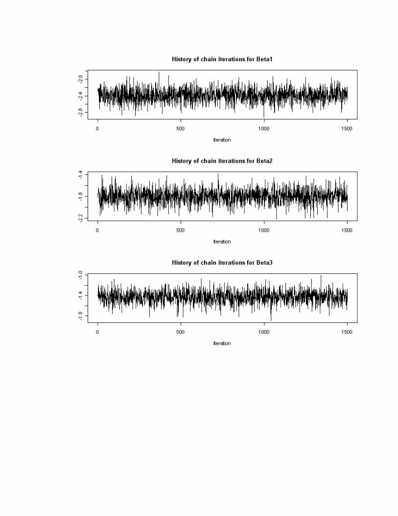
First, we use graphical techniques to asses the convergence and mixing of the chains.

One commonly used plot shows the history of sampled values at each iteration of the MCMC

algorithm. In this plot, the x-axis refers to the iteration number and the y-axis refers to the

sampled value. Using this kind of plot, lack of convergence is evidenced if one observes a trend

in the sampled values, meaning that the algorithm has not reached a stationary state. Further, if

the range of sampled values differs much through different intervals of iterations a bad mixing of

the chains is occurring. For example, the first 500 iteration give sampled values between, say,

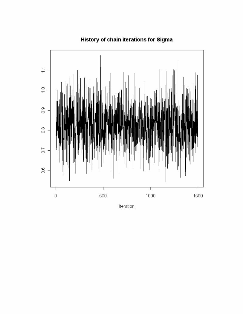
0.80 and 0.90 whereas iterations 501 to 1000 cover a different range of values. Figures 1 and 2

show the history of the chains’ iterations for the first three item parameters and the scale

parameterσ , respectively.

-----------------------------------------------------------------------------------------------------------

-

INSERT FIGURE 1 ABOUT HERE

-----------------------------------------------------------------------------------------------------------

-

-----------------------------------------------------------------------------------------------------------

-

INSERT FIGURE 2 ABOUT HERE

-----------------------------------------------------------------------------------------------------------

-

From the figures it can be seen that the chains don’t follow a clear trend meaning that

they would have converged at a stationary stage. Moreover, the range of sampled values

throughout the iterations is homogeneous meaning that the chains are mixing very well.

We also used the R̂ diagnostic to assess the convergence of the chains. The values of R̂

for all the parameters was less than or equal to 1.03 (see R output) for all fitted models so we

concluded that convergence had been established.

Once we are sure that the chains have converged, we can use samples from the posterior

distribution to obtain summaries. Table 1 shows the recovery results of parameter estimates. The

values in column WinBUGS correspond to the posterior mean of the parameter (i.e, the mean of

the 1500 values drawn from the posterior distribution).

---------------------------------------------------------------------------------------------------

INSERT TABLE 1 ABOUT HERE

----------------------------------------------------------------------------------------------------------

From the table it can be seen that the recovery is very good. The parameter estimates obtained by

WinBUGS were very close to the real values. Moreover, the WinBUGS results are very similar

to those obtained with MML estimation, the classical likelihood-based approach. This shows that

when using the Bayesian method estimation one can obtain the same level of accuracy as

traditional likelihood-based methods, provided that non-informative priors have been used.

Real data application: Rasch model

We use the “verbal aggression” data to exemplify the Bayesian estimation of both the Rasch and

the LLTM model. A full description of the data can be found in De Boeck and Wilson (2004).

The same number of chains as used in the simulation study was run and convergence was

assessed also in same way. The WinBUGS code to fit the Rasch model is shown in the

Appendix.

History plots of items and the scale parameter (not shown) gave evidence of convergence

and a good mixing of the chains. Also the R̂ values were all less than 1.004, meaning that

approximate convergence has been reached.

The item parameter estimates and the scale parameter of the random effects distribution

are shown in Table 2. This table contains the results using various softwares, and appears in

Chapter 11 of De Boeck and Wilson (2004). We have added the column “WinBUGS” in order to

compare the results with the other software.

-----------------------------------------------------------------------------------------------------------------

INSERT TABLE 2 ABOUT HERE

-------------------------------------------------------------------------------------------------------------------

It can be seen that the results are very similar when comparing the Bayesian approach and the

more classical approaches. As it was mentioned before, this similarity in the results is in a way

not surprising, since using noniformative priors, the posterior distribution is almost proportional

to the likelihood function, in which the likelihood-based method is fully based.

Second example: The LLTM

Chapter 2 of De Boeck and Wilson (2004) shows the fit of the LLTM model for the verbal

aggression data. We fit the model using the WinBUGS program. After checking convergence

and good mixing of the chains, the parameter estimates obtained are show in Table 3. This table

show the estimates using both the NLMIXED procedure from SAS, as reported by De Boeck and

Wilson (2004) and WinBUGS.

--------------------------------------------------------------------

INSERT TABLE 3 ABOUT HERE

--------------------------------------------------------------------

Again, the values are in good correspondence (almost identical). The estimate of the

2σ parameter is reported to be 1.86 (0.20) (De Boeck and Wilson, 2004) and the corresponding

estimated value in WinBUGS is 1.85 (0.19). It can be seen that the Bayesian estimates are

practically identical to the ones obtained using MML estimation.

Conclusions

This paper intended to serve as a brief introduction to the Bayesian method in the field of

IRT models and, mainly, to be a tutorial for the implementation of estimation algorithms using

freely available software. The Bayesian approach for the estimation of two IRT models (the

Rasch and the LLTM models) was presented. This estimation approach allows drawing samples

from the posterior distributions of the parameters we are interested on; it provides not only the

mean of the posterior but the complete distribution, permitting to obtain different kinds of

summary statistics such as quantiles, means, etc.

Besides the advantage of incorporating prior knowledge of the parameter, the Bayesian

method is a computationally more convenient way to estimate IRT models. The CML, MML

and JML methods have strengthness and weaknesess but as models are being extended to

accommodate more random effects (i.e., multidimensional traits or random item effects), they

become computationally infeasible.

The introduction and brief summary of the main ideas behind the Bayesian approach given

in this paper is not at all exhaustive, and this is why many good references were cited to guide

the reader in some topics.

Although only parametric models were considered here, there are methodologies and

software for the implementation of Bayesian semi-parametric models as well. The interested

reader is referred to Miyazaki and Hoshino (2009), and Jara (2007).

We have not considered here the issue of model selection, model checking, and goodness

of fit, thought there are Bayesian counterparts that account for it. For model selection under the

Bayesian approach, one may calculate Bayes factors (Kass & Raftery, 1995) and select the

model with the largest posterior probability given the data. Other possibility is the use of the

deviance information criteria (DIC; Spiegelhalter, Best, Carlin & Van der Linde, 2002), which is

a Bayesian counterpart of the more classical measures AIC and BIC. In assessing goodness of fit,

one may use posterior predictive checks (PPC; Gelman et. al, 2003) using samples from the

posterior distribution.

The Rasch and the LLTM models are only two of many other IRT models that can be fitted

using the Bayesian approach. Examples of more complex models in the family of IRT models

that have been estimated using Bayesian methods can be found in Janssen et al. (2000, 2004);

González, De Boeck, & Tuerlinckx (2008); González, Tuerlinckx and De Boeck (2009); among

others. These works give evidence that the Bayesian inference approach shows to be promising

for studying complex models in psychological research.

References

Baker, F., & Kim, S. (2004). Item response theory: Parameter estimation techniques (2nd ed.).

New York: Marcel Dekker.

Bates, D.M. & Sarkar, D. (2007). lme4: Linear mixed-effects models using S4 classes, R

package version 0.99875-6.

Carlin, B., Louis, T. (2000). Bayes and Empirical Bayes Methods for Data Analysis (2nd ed.).

Chapman & Hall/CRC.

Chib, S. and Greenberg, E. (1995). Understanding the Metropolis–Hastings Algorithm.

American Statistician, 49(4), 327–335.

Cowles, M., & Carlin, B. (1996). Markov chain Monte Carlo convergence diagnostics: a

comparative study. Journal of the American Statistical Association, 91, 883–904.

De Boeck, P. & Wilson, M. (2004). Explanatory Item Response Models: A Generalized Linear

and Nonlinear Approach. Springer-Verlag, New York.

Embretson, S. & Reise, S. (2000). Item response theory for psychologists. Mahwah, New Jersey:

Lawrence Erlbaum Associates.

Fischer, G. (1973). The linear logistic test model as an instrument in educational research. Acta

Psychologica, 3, 359-354.

Fischer, G. & Molenaar, I. (1995). Rasch models. Foundations, recent developments and

applications. New York: Springer.

Gelman, A. (2006). Prior distributions for variance parameters in hierarchical models. Bayesian

Analysis, 1, 515-533.

Gelman, A., Carlin, J., Stern, H., & Rubin, D. (2003). Bayesian data analysis (2nd ed.). New

York: Chapman and Hall.

Gelman, A., & Rubin, D. (1992). Inference from iterative simulation using multiple sequences

(with discussion). Statistical Science, 7, 457–511.

Gilks, W. R., Richardson, S., and Spiegelhalter, D. J. (eds.) (1995). Markov chain Monte Carlo

in practice. Chapman and Hall, New York

González, J., De Boeck, P., & Tuerlinckx, F. (2008). A double-structure structural equation

model for three-mode data. Psychological Methods, 13, 337-353.

González, J., Tuerlinckx, F., & De Boeck, P. (2009). Analyzing structural relations in

multivariate dyadic binary data. Applied Multivariate Research, 13, 77-92.

Hambleton, R., Swaminathan, H. & Rogers, H. (1991): Fundamentals of item response theory,

London, Sage.

Janssen, R., Schepers, J., & Peres, D. (2004). Models with item and item group predictors. In P.

De Boeck & M. Wilson (Eds.), Explanatory item response models: A generalized linear

and nonlinear approach (pp. 189–212). New York: Springer.

Janssen, R., Tuerlinckx, F., Meulders, M., & De Boeck, P. (2000). A hierarchical IRT model for

criterion-referenced measurement. Journal of Educational and Behavioral Statistics, 25,

285-306.

Jara, A. (2007). Applied Bayesian non- and semi-parametric inference using DPpackage. Rnews

7, 17–26.

Kass, R., & Raftery, A. (1995). Bayes factors. Journal of the American Statistical Association,

90, 773-796.

Lee, M. & Wagenmakers, E. (2005). Bayesian statistical inference in psychology: Comment on

Trafimow (2003). Psychological Review, 112, 662–668.

Lynch, S. (2007). Introduction to Applied Bayesian Statistics and Estimation for Social

Scientists. NY: Springer.

Matschinger, H. (2006), Estimating IRT models with gllamm, German Stata Users' Group

Meetings 2006, Stata Users Group.

Miyazaki and Hoshino (2009). A Bayesian Semiparametric Item Response Theory Model with

Dirichlet Process Priors. Psychometrika, 74, 375-393.

Molenaar, I. (1995). Estimation of Item Parameters. In Gerhard H. Fischer and Ivo W. Molenaar

(Eds.), Rasch models. Foundations, recent developments and applications (pages 39-52).

New York: Springer.1995.

Ntzoufras, I. (2009). Bayesian Modeling Using WinBUGS.

Pinheiro, J.C. & Bates, D.M. (2000). Mixed-effects models in S and S-PLUS. Springer, New

York.

Plummer, M., Best, N., Cowles, K., & Vines, K. (2006, March). CODA: Convergence diagnosis

and output analysis for MCMC. R News, 6, 7–11. Available from http://CRAN.R-

project.org/doc/Rnews/

Rabe-Hesketh, S., Skrondal, A. & Pickles, A. (2004). "GLLAMM Manual," U.C. Berkeley

Division of Biostatistics Working Paper Series 1160, Berkeley Electronic Press.

Rasch, G. (1960). Probabilistic models for some intelligence and attainment tests. Copenhagen,

Denmark: Danish institute for educational research.

Ravelle, W. (2008). Using R for psychological research: A simple guide to an elegant package.

Retrieved September 17, 2008, from http:/ /www.personality-project.org/r/

Rijmen, F., Tuerlinckx, F., De Boeck, P., & Kuppens, P. (2003). A nonlinear mixed model

framework for item response theory. Psychological Methods, 8, 185-205.

R Development Core Team (2009). R: A language and environment for statistical computing. R

Foundation for Statistical Computing, Vienna, Austria. ISBN 3-900051-07-0, URL

http://www.R-project.org.

Robert, C. and Casella, G. (2004). Monte Carlo Statistical Methods (2nd Edition). Springer-

Verlag: New York.

SAS Institute Inc. (2000). SAS 9.1.3 Help and Documentation, Cary, NC: SAS Institute Inc.,

2000-2004.

Sheu, C.-F., Chen, C.-T., Su, Y.-H., & Wang, W.-C. (2005). Using SAS PROC NLMIXED to fit

item response theory models. Behavior Research Methods, 37, 202-218

Spiegelhalter, D., Best, N., Carlin, B., & Van der Linde, A. (2002). Bayesian measures of model

complexity and fit. Journal of the Royal Statistical Society, B, 64, 583–639.

Spiegelhalter, D., Thomas, A., Best, N., & Lunn, D. (2003). WinBUGS version 1.4 user manual

[Computer software manual]. http://www.mrc-bsu.cam.ac.uk/bugs/winbugs/manual14.pdf.

StataCorp. (2009). Stata Statistical Software: Release 11. College Station, TX: StataCorp LP.

Stockman, F. (1977). Roll calls and sponsorship. A methodological analisys of third world group

formation in the United Nations. Leiden: Sijthoff.

Sturtz, S., Ligges, U., & Gelman, A. (2005). R2WinBUGS: A package for running WinBUGS

from R. Journal of Statistical Software, 12, 1–16. Available from http://www.jstatsoft.org

Tuerlinckx, F., Rijmen, F., Molenberghs, G., Verbeke, G., Briggs, D., Van den Noortgate, W.,

Meulders, M., & De Boeck, P. (2004). Estimation and software. In P. De Boeck & M.

Wilson (Eds.), Explanatory item response models: A generalized linear and nonlinear

approach (pp. 343-373). New York: Springer.

Appendix

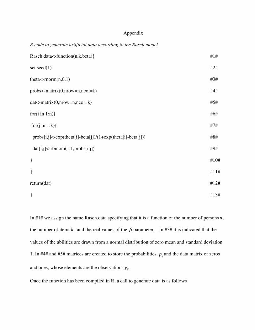
R code to generate artificial data according to the Rasch model

Rasch.data<-function(n,k,beta){ #1#

set.seed(1) #2#

theta<-rnorm(n,0,1) #3#

probs<-matrix(0,nrow=n,ncol=k) #4#

dat<-matrix(0,nrow=n,ncol=k) #5#

for(i in 1:n){ #6#

for(j in 1:k){ #7#

probs[i,j]<-exp(theta[i]-beta[j])/(1+exp(theta[i]-beta[j])) #8#

dat[i,j]<-rbinom(1,1,probs[i,j]) #9#

} #10#

} #11#

return(dat) #12#

} #13#

In #1# we assign the name Rasch.data specifying that it is a function of the number of persons ,

the number of items , and the real values of the

n

k β parameters. In #3# it is indicated that the

values of the abilities are drawn from a normal distribution of zero mean and standard deviation

1. In #4# and #5# matrices are created to store the probabilities and the data matrix of zeros

and ones, whose elements are the observations .

ijp

ijy

Once the function has been compiled in R, a call to generate data is as follows

data.set1=Rasch.data(500,11,seq(-2.5,2.5,0.5))

where data.set1 is the object in which the data are stored.

R-WinBUGS code to fit the models

We present the used code to fit the models presented in the paper. This code can easily be

adapted to fit other models. For a detailed explanation of the R2WinBUGS package the reader is

referred to Sturtz, Ligges, and Gelman (2005).

Preliminaries

1. Install WinBUGS if it is not already installed in your system. The program and all

the information for installation can be found at http://www.mrc-bsu.cam.ac.uk/bugs/

2. Install R and the R2WinBUGS package if they are not already installed. R and all

available packages can be found at http://www.r-project.org/

3. Write the WinBUGS code of the model in the file file.txt (see below)

4. Run the R script to call WinBUGS from R (see below)

WinBUGS code

Copy and paste the following WinBUGS code to create the Rasch Model rd.txt file.

model; #1#

{ #2#

for(i in 1:n){ #3#

theta[i]~dnorm(0,tau) #4#

for(j in 1:k){ #5#

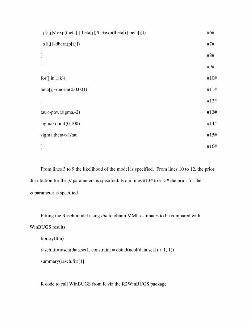
p[i,j]<-exp(theta[i]-beta[j])/(1+exp(theta[i]-beta[j])) #6#

x[i,j]~dbern(p[i,j]) #7#

} #8#

} #9#

for(j in 1:k){ #10#

beta[j]~dnorm(0,0.001) #11#

} #12#

tau<-pow(sigma,-2) #13#

sigma~dunif(0,100) #14#

sigma.theta<-1/tau #15#

} #16#

From lines 3 to 9 the likelihood of the model is specified. From lines 10 to 12, the prior

distribution for the β parameters is specified. From lines #13# to #15# the prior for the

σ parameter is specified

Fitting the Rasch model using ltm to obtain MML estimates to be compared with

WinBUGS results

library(ltm)

rasch.fit=rasch(data.set1, constraint = cbind(ncol(data.set1) + 1, 1))

summary(rasch.fit)[1]

R code to call WinBUGS from R via the R2WinBUGS package

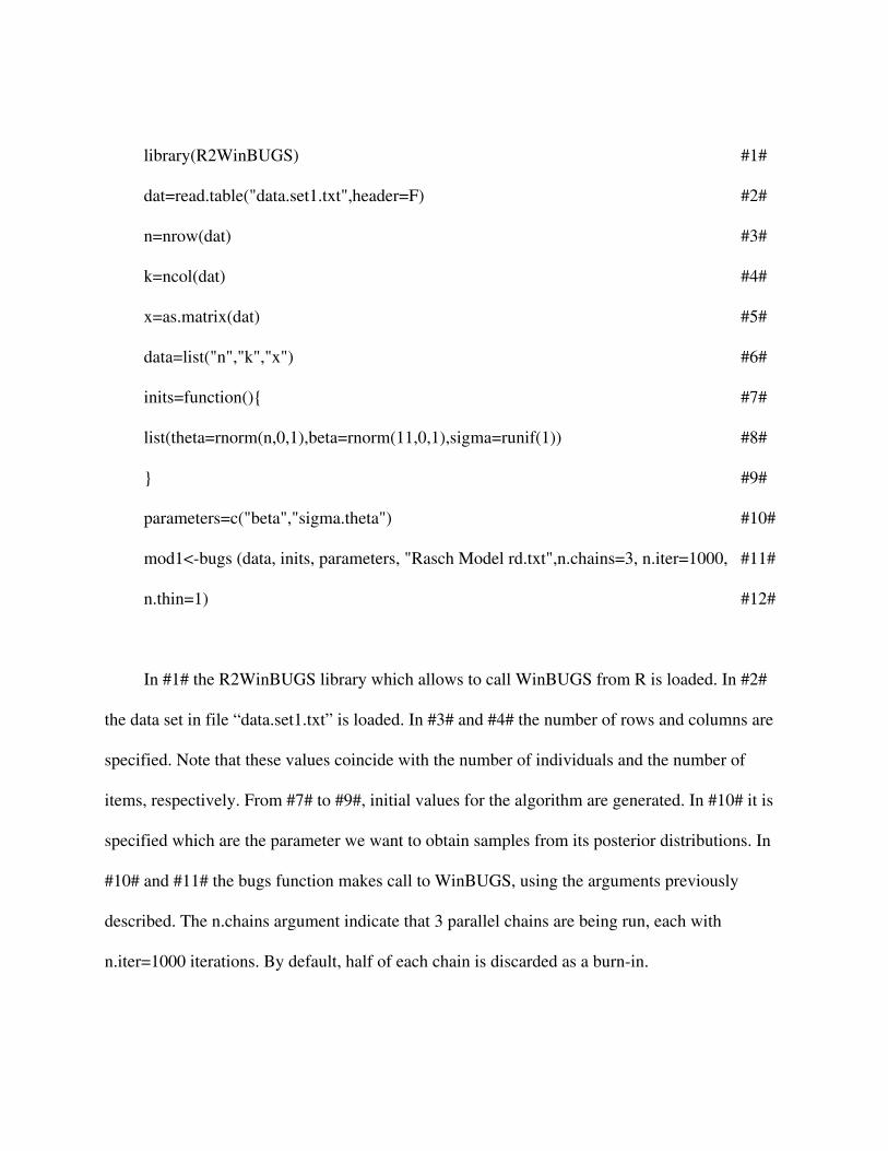
library(R2WinBUGS) #1#

dat=read.table("data.set1.txt",header=F) #2#

n=nrow(dat) #3#

k=ncol(dat) #4#

x=as.matrix(dat) #5#

data=list("n","k","x") #6#

inits=function(){ #7#

list(theta=rnorm(n,0,1),beta=rnorm(11,0,1),sigma=runif(1)) #8#

} #9#

parameters=c("beta","sigma.theta") #10#

mod1<-bugs (data, inits, parameters, "Rasch Model rd.txt",n.chains=3, n.iter=1000, #11#

n.thin=1) #12#

In #1# the R2WinBUGS library which allows to call WinBUGS from R is loaded. In #2#

the data set in file “data.set1.txt” is loaded. In #3# and #4# the number of rows and columns are

specified. Note that these values coincide with the number of individuals and the number of

items, respectively. From #7# to #9#, initial values for the algorithm are generated. In #10# it is

specified which are the parameter we want to obtain samples from its posterior distributions. In

#10# and #11# the bugs function makes call to WinBUGS, using the arguments previously

described. The n.chains argument indicate that 3 parallel chains are being run, each with

n.iter=1000 iterations. By default, half of each chain is discarded as a burn-in.

Author note

Jorge González, Measurement Center MIDE UC, Pontificia Universidad Católica de Chile,

Chile.

The author wants to thank Veronica Santelices, for her valuable help and suggestions concerning

the manuscript.

Correspondence should be addressed to Jorge González, Centro de Medición MIDE UC,

Pontificia Universidad Católica de Chile, Av. Vicuña Mackenna 4860 Macul Santiago, Chile.

Tel.: +56 2 3541730; e-mail: jagonzal@uc.cl

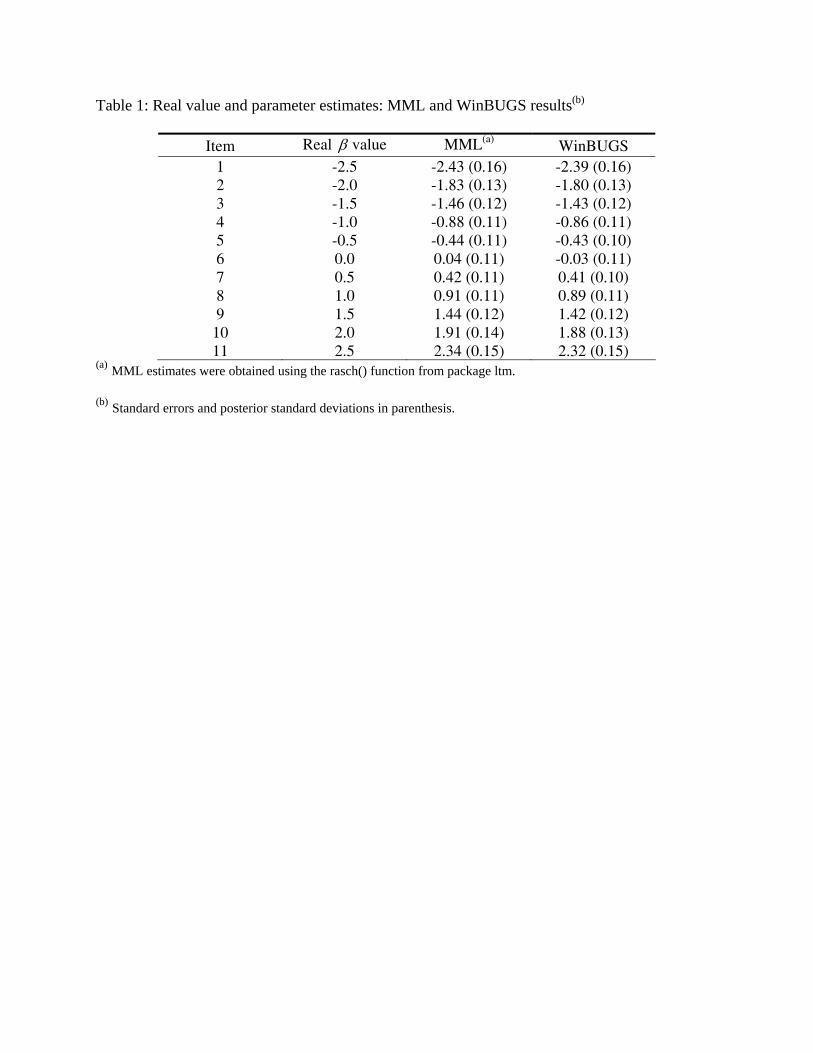
Table 1: Real value and parameter estimates: MML and WinBUGS results(b)

Item Real β value MML(a) WinBUGS 1 -2.5 -2.43 (0.16) -2.39 (0.16) 2 -2.0 -1.83 (0.13) -1.80 (0.13) 3 -1.5 -1.46 (0.12) -1.43 (0.12) 4 -1.0 -0.88 (0.11) -0.86 (0.11) 5 -0.5 -0.44 (0.11) -0.43 (0.10) 6 0.0 0.04 (0.11) -0.03 (0.11) 7 0.5 0.42 (0.11) 0.41 (0.10) 8 1.0 0.91 (0.11) 0.89 (0.11) 9 1.5 1.44 (0.12) 1.42 (0.12) 10 2.0 1.91 (0.14) 1.88 (0.13) 11 2.5 2.34 (0.15) 2.32 (0.15)

(a) MML estimates were obtained using the rasch() function from package ltm.

(b) Standard errors and posterior standard deviations in parenthesis.

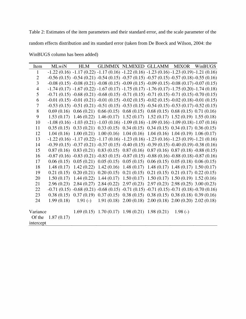
Table 2: Estimates of the item parameters and their standard error, and the scale parameter of the

random effects distribution and its standard error (taken from De Boeck and Wilson, 2004: the

WinBUGS column has been added)

Item MLwiN HLM GLIMMIX NLMIXED GLLAMM MIXOR WinBUGS 1 -1.22 (0.16) -1.17 (0.22) -1.17 (0.16) -1.22 (0.16) -1.23 (0.16) -1.23 (0.19) -1.21 (0.16) 2 -0.56 (0.15) -0.54 (0.21) -0.54 (0.15) -0.57 (0.15) -0.57 (0.15) -0.57 (0.18) -0.55 (0.16) 3 -0.08 (0.15) -0.08 (0.21) -0.08 (0.15) -0.09 (0.15) -0.09 (0.15) -0.08 (0.17) -0.07 (0.15) 4 -1.74 (0.17) -1.67 (0.22) -1.67 (0.17) -1.75 (0.17) -1.76 (0.17) -1.75 (0.20) -1.74 (0.18) 5 -0.71 (0.15) -0.68 (0.21) -0.68 (0.15) -0.71 (0.15) -0.71 (0.15) -0.71 (0.15) -0.70 (0.15) 6 -0.01 (0.15) -0.01 (0.21) -0.01 (0.15) -0.02 (0.15) -0.02 (0.15) -0.02 (0.18) -0.01 (0.15) 7 -0.53 (0.15) -0.51 (0.21) -0.51 (0.15) -0.53 (0.15) -0.54 (0.15) -0.53 (0.17) -0.52 (0.15) 8 0.69 (0.16) 0.66 (0.21) 0.66 (0.15) 0.68 (0.15) 0.68 (0.15) 0.68 (0.15) 0.71 (0.16) 9 1.53 (0.17) 1.46 (0.22) 1.46 (0.17) 1.52 (0.17) 1.52 (0.17) 1.52 (0.19) 1.55 (0.18) 10 -1.08 (0.16) -1.03 (0.21) -1.03 (0.16) -1.09 (0.16) -1.09 (0.16) -1.09 (0.18) -1.07 (0.16) 11 0.35 (0.15) 0.33 (0.21) 0.33 (0.15) 0.34 (0.15) 0.34 (0.15) 0.34 (0.17) 0.36 (0.15) 12 1.04 (0.16) 1.00 (0.21) 1.00 (0.16) 1.04 (0.16) 1.04 (0.16) 1.04 (0.19) 1.06 (0.17) 13 -1.22 (0.16) -1.17 (0.22) -1.17 (0.16) -1.23 (0.16) -1.23 (0.16) -1.23 (0.19) -1.21 (0.16) 14 -0.39 (0.15) -0.37 (0.21) -0.37 (0.15) -0.40 (0.15) -0.39 (0.15) -0.40 (0.19) -0.38 (0.16) 15 0.87 (0.16) 0.83 (0.21) 0.83 (0.15) 0.87 (0.16) 0.87 (0.16) 0.87 (0.18) -0.88 (0.15) 16 -0.87 (0.16) -0.83 (0.21) -0.83 (0.15) -0.87 (0.15) -0.88 (0.16) -0.88 (0.18) -0.87 (0.16) 17 0.06 (0.15) 0.05 (0.21) 0.05 (0.15) 0.05 (0.15) 0.06 (0.15) 0.05 (0.18) 0.06 (0.15) 18 1.48 (0.17) 1.42 (0.22) 1.42 (0.16) 1.48 (0.17) 1.48 (0.17) 1.48 (0.17) 1.50 (0.17) 19 0.21 (0.15) 0.20 (0.21) 0.20 (0.15) 0.21 (0.15) 0.21 (0.15) 0.21 (0.17) 0.22 (0.15) 20 1.50 (0.17) 1.44 (0.22) 1.44 (0.17) 1.50 (0.17) 1.50 (0.17) 1.50 (0.19) 1.52 (0.16) 21 2.96 (0.23) 2.84 (0.27) 2.84 (0.22) 2.97 (0.23) 2.97 (0.23) 2.98 (0.25) 3.00 (0.23) 22 -0.71 (0.15) -0.68 (0.21) -0.68 (0.15) -0.71 (0.15) -0.71 (0.15) -0.71 (0.18) -0.70 (0.16) 23 0.38 (0.15) 0.37 (0.19) 0.37 (0.15) 0.38 (0.15) 0.38 (0.15) 0.38 (0.18) 0.39 (0.16) 24 1.99 (0.18) 1.91 (-) 1.91 (0.18) 2.00 (0.18) 2.00 (0.18) 2.00 (0.20) 2.02 (0.18)

VarianceOf the

intercept 1.87 (0.17)

1.69 (0.15) 1.70 (0.17) 1.98 (0.21) 1.98 (0.21) 1.98 (-)

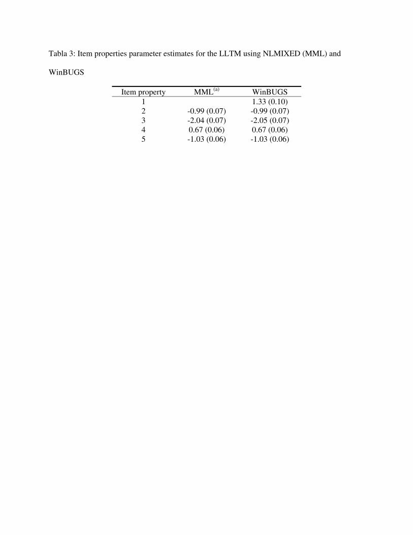
Tabla 3: Item properties parameter estimates for the LLTM using NLMIXED (MML) and

WinBUGS

Item property MML(a) WinBUGS 1 1.33 (0.10) 2 -0.99 (0.07) -0.99 (0.07) 3 -2.04 (0.07) -2.05 (0.07) 4 0.67 (0.06) 0.67 (0.06) 5 -1.03 (0.06) -1.03 (0.06)

Figure captions

Figure 1. History of chain iterations for the first three item parameters

Figure 2. History of iterations for the σ parameter.