BAYESIAN METHODOLOGY FOR

IMPOSING INEQUALITY CONSTRAINTS

ON A LINEAR EXPENDITURE SYSTEM

WITH DEMOGRAPHIC FACTORS

William E. Gfiffiths and Duangkamon Chotikapanich

No. 93 -December 1996

ISSN 0 157 0188

ISBN 1 86389 398 9

BAYESIAN METHODOLOGY FOR IMPOSINGINEQUALITY CONSTRAINTS ON A LINEAR

EXPENDITURE SYSTEM WITH DEMOGRAPHICFACTORS

William E. GriffithsUniversity of New England

and

Duangkamon ChotikapanichCurtin University of Technology

1. INTRODUCTION

Bayesian econometrics started to gain in popularity following the publication of

Zellner (1971), and has subsequently been utilized in many applications (Koop, 1994).

There has been a lively and broad-ranging debate over the merits of Bayesian versus

sampling theory inference (see, for example, Zellner, 1988 and Poirier, 1995).

However, one of the generally-recognized desirable characteristics of the Bayesian

approach is that it provides a formal mechanism for including prior information about

unknown parameters. Since economists frequently have prior information about the

parameters in their economic relationships, this characteristic is particularly appealing.

"Mixed estimation" (Theil and Goldberger, 1961 and Theil, 1963) provided one way of

including prior information on parameters, but it is less flexible than the Bayesian

approach, and it does not fit neatly into either the Bayesian or sampling theory

paradigms.

One of the major obstacles to the application of Bayesian econometrics has been

the perceived need for numerical integration. A common way to present results from a

Bayesian investigation is to provide graphs of the marginal posterior probability density

functions (p.d.f.s) for each of the unknown parameters in which we are interested.

Instead of following the sampling theory approach of presenting a point estimate and

its corresponding standard error, the Bayesian approach summarizes information about

an unknown parameter in terms of a p.d.f, that describes how likely (in a subjective

probabilistic sense) different values of the parameter are. See Griffiths et al. (1993,

Chapters 24 and 25) for an introductory exposition. In order to present information in

this way, it is necessary to derive marginal posterior p.d.f.s for each of the unknown

parameters from the joint posterior p.d.f, for all the parameters. This process means

that unwanted parameters must be integrated out of the joint posterior p.d.f. If

analytical integration is not possible, or the dimension of the joint posterior p.d.f, is

greater than three, making numerical integration impractical, some other solution must

be found. One such solution, which has led to an enormous explosion in Bayesian

literature over the last five years, is the use of Markov Chain Monte Carlo (MCMC)

techniques. These techniques provide a way of drawing observations from the joint

posterior p.d.f. Once some observations have been drawn, they can be used to

2

construct histograms as estimates of the marginal posterior p.d.f.s. Since observations

are drawn artificially using computer software, we can make estimated marginal

posterior p.d.f.s as accurate as we like, by drawing as many observations as are

required. Marginal posterior p.d.f.s are not the only way of presenting information that

utilizes MCMC-estimated integrals. Posterior means and standard deviations which are

the Bayesian counterparts of sampling theory point estimates and standard errors often

take the form of intractable integrals. These quantifies can be readily estimated using

the sample means and standard deviations of the MCMC-generated observations.

There are two main MCMC techniques, Gibbs sampling, and the Metropolis-Hastings

algorithm. For access to the literature, and an appreciation of the wide variety of

applications, see Albert and Chib (1996), Chib and Greenberg (1996), Tanner (1993)

and Gilks et al. (1996).

The availability of MCMC techniques provides new opportunities for applying

Bayesian econometrics in general, and, in particular, for including prior information

into estimation procedures. One of these opportunities is taken up in this paper; we

i~ustrate how the Metropolis-Hastings algorithm can be utilized to include prior

information in the form of inequality constraints into Bayesian estimation of a linear

expenditure system. Although linear expenditure systems typically involve "subsistence

parameters" which, based on the corresponding utility function, should be exceeded by

all sample expenditures, to our knowledge there have not been any studies which

incorporate this constraint into an estimation procedure. We fill this gap in the

literature. Also, including demographic factors into the linear expenditure system raises

questions about the relative consumption of people in different age-gender categories.

Our estimation methodology shows how prior information on relative consumption can

be included in the form of inequality constraints on parameters.

Engel (expenditure) functions which relate expenditure on individual commodity

groups to total expenditure are functions commonly estimated in economics. For

examples, see Bewley (1982) and Giles and Hampton (1985), and references therein.

When estimating such functions from household data, a question that must be faced is

how to model households with different household compositions. Simply treating

expenditures on a per capita basis ignores the fact that the expenditure requirements

for particular commodities may be less for additional members of the household than

they are for (say) the first adult member. This problem has been overcome by

introducing so called demographic factors into Engel or expenditure functions. For a

review of the various suggestions for including demographic factors, see Pollak and

Wales (1981, 1992). One of the early suggestions ~rais and Houthakker, 1955) was to

deflate expenditure on each commodity by a commodity-specific household scale

which measured the "size" of that household relative to expenditure on the commodity

by some reference household; total expenditure was deflated using a general scale.

Attempts to introduce demographic factors in a manner consistent with utility theory

were first made by Batten (1964) and considered further by Pollak and Wales (1981,

1992). An extensive Australian study that utilizes time-series and cross-sectional data

for including demographic variables and develops methodology for cross-sectional

aggregation is that of Perkins (1984).

A commonly used system of expenditure functions is the linear expenditure

system (LES) that is derived from a so called Stone-Geary utility function. See, for

example, Powell (1974). In this study we use this linear expenditure system as the basis

for estimating functions from cross-section household budget data where there is no

price variation. We use the Prais-Houthakker procedure to introduce demographic

factors and present the modified utility function from which the new LES can be

derived. Linear Engel functions have been recognized as a particularly restrictive

functional form specification. See, for example, Rimmer and Powell (1994). However,

they do provide a convenient framework to illustrate the power of the methodology,

and they are still popular for providing empirical results for policy analysis (Binh and

Whiteford, 1990 and Clements et al., 1996). Also, our final model is one which is very

nonlinear in the parameters, and so our methodology can be readily adapted to

alternative nonlinear models. One difficulty with estimating the LES when there is no

price variation is that not all of the parameters are identified. A further problem is that

parameter estimates may turn out to be inconsistent with relationships implied by the

utility function. These two problems are solved using a Bayesian estimation procedure

that imposes inequality constraints consistent with the utility function. Also, we

illustrate how to take advantage of prior information on elasticities and on the relative

magnitudes of scales for households with differing compositions. The possibility of

exact inference for nonlinear functions of interest is another advantage of the Bayesian

approach. In Section 2 we describe the Prais-Houthakker method of including

demographic factors into a LES, give the corresponding utility function and discuss the

parameters and constraints on them; a description of the Thai data to which the

methods are applied also appears in this section. Both maximum likelihood and

Bayesian estimation are outlined in Section 3 along with further details about the

inequality constraints on the parameters. The results are presented in Section 4 and

conclusions drawn in Section 5.

2. PRAIS-HOUTHAKKER MODEL

Maximizing the utility function

U(ql,qz .....q.)=~.,~log(q~-a~) 13j >0, qj->aj, ~13~=1 (1)j=l J

subject to the budget constraint ~..~p~q~ = x leads to the well-known Klein-Rubin

linear expenditure system

= + (2)\ k

where pj and q_i denoted prices and quantities, respectively, e~. = pjq~ is expenditure on

the jth commodity, x is total expenditure, and at = p~a~ and 13~ are parameters. The

parameter (xj- is often interpreted as the subsistence expenditure for the jth commodity,

and (x-~.%) as supernumerary expenditure. For this interpretation to be

meaningful the constraints o9 > 0 are necessary. Pollak (1971) and Pollak and Wales

(1978) note that (1) is still a valid utility function for c~j < 0 and prefer to let the signs

of the c~ be determined empirically. Also, it can be shown that an inelastic demand

implies o9 > 0 and an elastic demand implies c~ < 0. In our Bayesian analysis in this

paper we impose constraints of the form c9 > 0 or 09 < 0 based on a priori beliefs

concerning whether demand is inelastic or elastic.

To introduce demographic factors into this system, the Prais-Houthakker (1955)

procedure replaces the above system (2) by

---%+13i - otk (3)m~

5

where

mj = weighted size or adult-equivalent size of the household corresponding to

the jth commodity. This quantity is also known as a household

equivalence scale for the.]th commodity;

m0 = weighted size or adult-equivalent size of the household corresponding to

total expenditure.

This system expresses the equation in terms of per adult-equivalent expenditure.

Typically, mj. and mo are functions of the age and gender composition of the household.

Prais and Houthakker mainly considered double-log and semi-log equations rather than

the linear one in equation (3), and they did not concern themselves with utility theory

and the budget constraint. Using the Prais-Houthakker procedure, but a different

functional form to that in (3), Muellbauer (1980) used the budget constraint to define

m0 in terms of the mj. and total expenditure. Pollak and Wales (1981) called this process

the "modified" Prais-Houthakker procedure and illustrated its application to a linear

expenditure system like that in (3). Specifically, rearranging (3) and summing over

commodities yields

or

m0 -~ (4)

Substituting this mo into system (2), the expenditure system can be written as:

~ 13~rnk[3,m, (ej = c~jm~ + x - ~c%rnz (5)k

Equation (5) can be viewed as the linear expenditure system with demographic factors

mj included via the modified Prais-Houthakker method. Pollak and Wales (1981)

describe this and other methods for including demographic factors, including

demographic translating, demographic scaling and a "Gorman procedure" that includes

translating and scaling as special cases; they relate these methods to corresponding

changes in the direct and indirect utility functions. Batten (1964) was the first author to

suggest demographic scaling in the context of utility theory.

Given that Prais-Houthakker (1955) introduced demographic factors without

considering the nature of any corresponding utility function, it is natural to ask what

kind of utility function will lead to the system in (5). The appropriately modified

version of (1) is

U(qi,q2,...,q,)= X~3jrajlog( qJ -ajl ~3~ > O, qj" > aj (6)j k.mj j mj

To show that the utility function (6) leads to the modified linear system (5) we

maximize (6) subject to budget constraint ~p~q~ = x. This process leads to

ej = pjqj = pja~mj + ~.,~3~mk x - ~p~akm~ (7)

k

For the special case where cross-section data are used, the price variables py are

constant in which case the expenditure system becomes that in (5), with % = pjaj.

The direct additive utility function (6) has an interesting interpretation. The term

~3~ log((qj/mj)- a j) can be viewed as the relative utility from thejth commodity, in

adult-equivalent terms. Weighting this quantity by my, the number of equivalent adults,

gives it an interpretation as the household utility from the jth commodity. Summing

over all commodities gives it a total household utility interpretation. This interpretation

can be contrasted with the Barten procedure, which Pollack and Wales (1981) called

"demographic scaling". Demographic scaling modifies the original demand system by

replacing q~. by qj/mj, the effective quantity, and replacing py by pjmy, the effective

price. In this case the LES (1) becomes

pjqj = p~mfl~ +~3.~(x- ~p~m~a~)

This system of demand functions can be derived from a direct additive utility function

of the form:

U(q~,q2,...,q,) = ~3~ log( q~ - a~)

This utility function is similar to the one in (6) except that it is a per adult-equivalent

utility function, rather than a household utility function.

7

The parameters of the modified LES

Two advantages of the Bayesian approach to inference, particularly in the

context of the model we are investigating, are its ability to include prior inequality

constraints on the parameters, and its ability to make finite sample inferences about

nonlinear functions of the parameters. It is useful, therefore, to examine the

parameters, possible constraints, and nonlinear functions of interest.

(a) The 13’s

An obvious constraint that we have already imposed via our definition of m0 is

the budget constraint ~ e~ = x. A less obvious constraint that seems intuitively

reasonable is a per adult-equivalent adding up constraint that the sum of adult-

equivalent expenditures over all commodity groups should be equal to adult-

equivalent total expenditure. That is:

~ rn~ m0

If we apply this result to (3) we obtain:

For this result to be true for all households we require ~ 13, = 1. Moreover, the

utility ordering in (6) is preserved if we divide this equation by a constant.

Dividing by ~ 13~ would ensure that a set of newly defined 13k would satisfy the

constraint ~ 13 ~ = 1. We therefore also have the constraint 0 _< 13.~ _< 1.

(b) The mj.’s and m0

At this point we need to introduce more notation. Let all household members be

classified into G age-gender categories (g = 1,2,...,G). We assume that the

household equivalence scale for thejth commodity is related to the composition

of the household through the equation

/’/g = the number of people in the gth age-gender category.

the specific scale that measures the weight given to an individual

belonging to the gth age-gender category with respect to consumption of

8

thejth commodity group. This weight is estimated according to the share

of the individual in the consumption cost of the jth specific item.

Typically, the ~5~ are normalized in some way. We set ~51! = 1 for all

commodity groups, where g = 1 refers to the adult category. Thus,

(g ~ 1) can be viewed as the additional expenditure on commodity group

j needed for an additional person in age-gender category g. Typically, we

have prior inequality information about the 5~. For example, in food

consumption, we expect the ~5~ for children to be less than that for adults.

Inequalities of this nature are introduced into the Bayesian estimation

procedure.

From equations (4) and (5) it is clear that the general houshold scale m0 is

a nonlinear function of the parameters ([3j, ctl., 5~.); Bayesian estimation

permits finite sample inference about this nonlinear function.

(c) The c~’s:

In the original sense of the LES, ctj is defined as the subsistence level of

expenditure of thejth commodity. However, the sign of o~: also dictates whether

the jth commodity is price elastic or price inelastic. A positive ct~- indicates that

demand for the jth commodity is inelastic and a negative ctl. indicates otherwise.

To demonstrate this fact let

From (7) we have

)Taking the derivative of q~- with respect to pC the price elasticity can be derived

asl

(9)

9

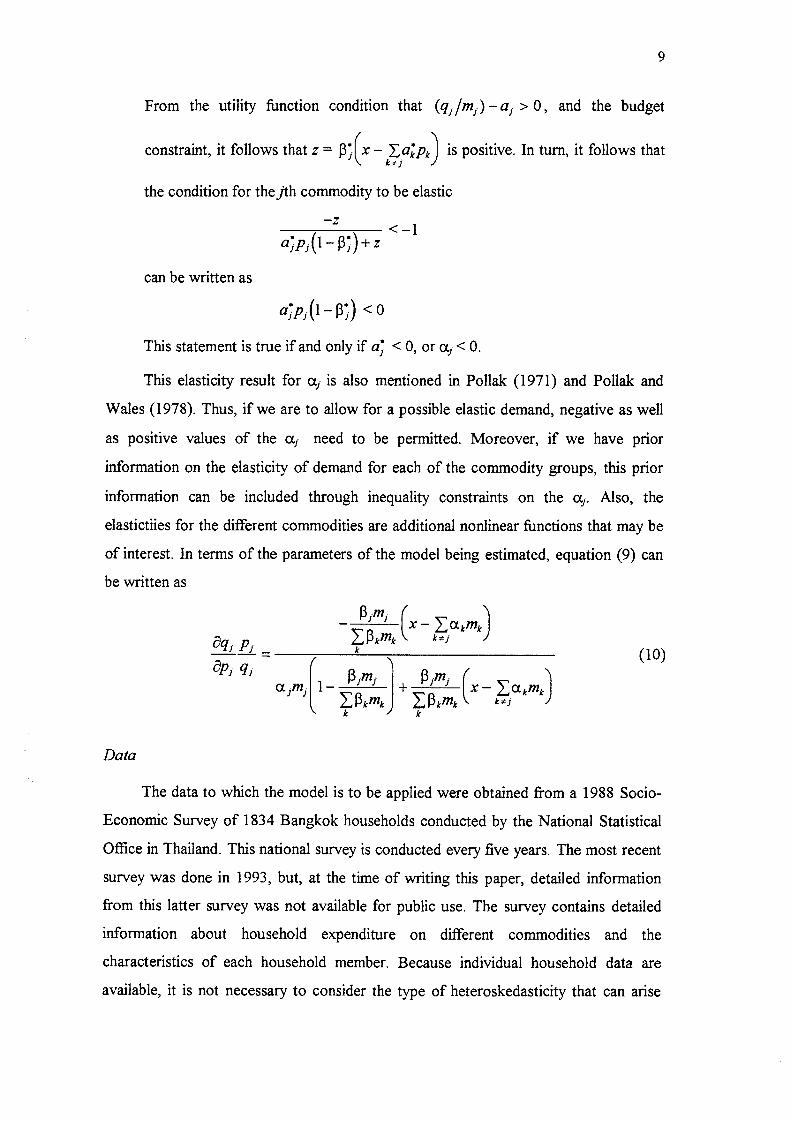
From the utility function condition that (q jim j)-aj > 0, and the budget

t"constraint, it follows that z = 13].Ix- Y~a;p, is positive. In turn, it follows that

the condition for thejth commodity to be elastic

-Z

a;p~(1-13;) + z

can be written as

< 0This statement is true if and only if a~ < O, or ctj < O.

This elasticity result for ctj is also mentioned in Pollak (1971) and Pollak and

Wales (1978). Thus, if we are to allow for a possible elastic demand, negative as well

as positive values of the c~j. need to be permitted. Moreover, if we have prior

information on the elasticity of demand for each of the commodity groups, this prior

information can be included through inequality constraints on the ctj-. Also, the

elastictiies for the different commodities are additional nonlinear functions that may be

of interest. In terms of the parameters of the model being estimated, equation (9) can

be written as

Data

The data to which the model is to be applied were obtained from a 1988 Socio-

Economic Survey of 1834 Bangkok households conducted by the National Statistical

Office in Thailand. This national survey is conducted every five years. The most recent

survey was done in 1993, but, at the time of writing this paper, detailed information

from this latter survey was not available for public use. The survey contains detailed

information about household expenditure on different commodities and the

characteristics of each household member. Because individual household data are

available, it is not necessary to consider the type of heteroskedasticity that can arise

10

when only grouped data are available (Kakwani, 1977). To simplify the computations,

the commodities are classified into three commodity groups (j = 1,2,3); the household

members are classified into three age groups (g = 1,2,3) as follows:

: Household membersg~ 1;213

Commodities consumedj = li213

g= 1 adult j = 1 foodg = 2 extra adult j = 2 other necessitiesg = 3 children under the age of 15 j = 3 non-necessities

The commodities category "other necessities" includes clothing, housing and medical

expenditure. This is a greater level of aggregation than is usually considered in studies

of this type. However, keeping the number of commodity groups small enables us to

focus on the estimation methodology.

3. ESTIMATION

To avoid heteroskedasticity it is common to estimate equation (5) in budget

share form. Making this transformation, including a subscript to denote the ith

observation, and including a random error term u~i, leads to the equation

O~" jmji k

w~i = fji(ot.,~,~3)+u~i - + +u~i (11)k

= eji/xi . A check for heteroskedasticity that we mention later suggestedwhere W ji

that any potential heteroskedasticity had been eliminated.

Equation (11) represents a system of 3 equations, one for each expenditure share

(j = 1,2,3). For the purpose of estimation, only the first two equations are considered

because the adding up condition ~w~ = 1 makes the third equation redundant. In

vector notation the unknown parameters in the i’u-st two equations are

c~ = (%,0%,a3)’ (12a)

15 = (1~1,[52)’ (12b)

5 : (521,531,522,832,523,533)1 (12c)

11

Equation (12c) contains 6 rather than 9 unknown parameters because the first adult is

adopted as the standard unit of comparison. That is, equation (8) can be written as

where

n2i

n3i

mji = 1 + 8,_jn2i +83jn3i j= 1,2,3 (13)

= number of the extra adults in the ith household

= number of children in the ith household.

Note also that, once 131 and 132 are estimated, 133 can be estimated from (1 - 13! - 132).

Furthermore, the equations for the ftrst two commodities in (11) contain not only the

~g~ that relate to the first and second commodities, but also ~3 and ~33, the adult

equivalence scales for the third commodity. Thus, estimating the first two equations

gives estimates of all the 13’s and g’s. However, it turns out that not all of the c9 are

identified and we cannot estimate all three of them without some kind of restriction.

Maximum Likelihood Estimation

For discussion of the estimation stage, it is convenient to write the model in

matrix algebra notation as

w = f + u (14)

where w’ = (w~,w~) with w’i = (wjl,wj: .....WaH), f and u are similarly partitioned, and H

= 1834 is the number of households. We assume that u - N(0,Z ® In) where ~1 is the

(212) error covariance matrix

Let 0 = (ot’,l~’,8’)’. The likelihood function can be written as [see Judge et al. (1985,

p.478) and Judge et al. (1988, p.553)]

p(wlO, Z)~ lzl-S/: exp{-~(w - f )" (Z-l ® I z4 Xw - ’)}

= IzI-H/2 exp{-½ tr(SZ-1 )} (15)

where S is a (2×2) matrix with (],k)th element equal to

Six =[wk - fk(0)] [w/- fi(0)] (16)

12

and tr(.) refers to the trace of a matrix. The first line in equation (15) is the traditional

way of writing the likelihood function in the econometric literature. The second line is

a useful expression for different aspects of Bayesian inference.

Given that equation (15) represents the normal likelihood function for a set of

nonlinear seemingly unrelated regressions, it appears straightforward to apply a

standard econometric software package, such as SHAZAM (White, 1993), to find the

maximum likelihood estimate for 0. However, if we try this strategy, we discover that

unique maximizing values for I~ and/~ can be found, but not so for et. Without an

additional restriction, all three elements in ct cannot be identified. The restrictions

imposed to overcome this problem are discussed in the section describing the results.

With these restrictions imposed, the maximum likelihood estimates are readily

calculated using SHAZAM.

Bayesian Estimation

Associated with maximum likelihood estimation are three difficulties that can be

readily overcome with the Bayesian approach. First, the identifying restrictions

imposed on the ctj’s are somewhat arbitrary. Second, prior inequality information that

exists on the ct’s and 6’s is not utilized. Third, exact inference for nonlinear functions of

the parameters such as m0 and the elasticities is not possible. The necessary steps to

proceed with Bayesian estimation are (1) specification of a prior p.d.f, that

accommodates the available prior inequality information, (2) derivation of the joint

posterior p.d.f, for all the unknown parameters through application of Bayes’ Theorem,

and (3) isolation of information from the joint posterior p.d.f. (marginal posterior

p.d.£s, posterior means and standard deviations) so that meaningful results can be

presented.

For specification of a prior p.d.£ we begin with each of the elements in I], ~5 and

et. They are assigned uniform priors with inequality restrictions. The uniform inequality

restricted prior implies that values of the parameters that do not satisfy the inequalities

are impossible, and that all values that do satisfy the inequalities are equally likely.

Clearly, nobody would truly regard all feasible parameter values as equally likely.

However, specifying a prior p.d.f, that is not uniform, and that accommodates the fact

that some parameter values are more or less likely than others, introduces

13

disagreement between different investigators. What is an acceptable prior p.d.f, for one

person may not be so for somebody else. Using uniform prior p.d.f.s does not

introduce information that is not generally acceptable, and it lets the data tell us what

parameter values are more or less likely within the feasible parameter range. The

restrictions imposed on the elements of 13 and 6 are as follows.

0--<821--< 1

As discussed above, this restriction comes from the utility

function or from a per unit adding-up constraint.

Expenditure on food for an additional adult is positive but

less than that for the first adult.

0 ~ 631 ~ Expenditure on food for a child is positive but less than that

for the additional adult.

0 --< 622 ~ 1

0 ~ 632 ~ 622

The additional adult expenditure on other necessities is

positive but less than that of the first adult.

Expenditure on other necessities for a child is positive but

less than that for an additional adult.

0_<623_< 1

0 --< 633 ~ 623

Expenditure on nonnecessities for the additional adult is

positive but less than that of the first adult.

Expenditure on nonnecessities for a child is positive but less

than that of the additional adult.

Restrictions on the elements of ~x are important. Without them the posterior

density function for ~x would be improper; this outcome is the Bayesian counterpart of

maximum likelihood estimates that are unidentified. There are two sources of

information that can be used to restrict the ctj. The first is a presumption about the

elasticities. We assume that the demands for food and other necessities are inelastic

and that the demand for non_necessities is elastic. Thus, we have czl > 0, Ct2 > 0 and

% < 0. The other source of information is from the utility function. The form of the

utility function requires (qj/mj.) > aj, or, equivalently, (p~qj/m:) > pja~. In terms of

the parameters, we have

14

ej>

1 + 82~n2 + 83~n3

For this constraint to hold for all observations in the sample, we require

{eji

,} (17)o~j < ~in ,1+�~2jn2i +~)3jn3i

Combining this result with that from the elasticities, we have the inequalities

O< ~xl< m, in{1 + ~.ln~i

0 < c% < min 1 + gz~n2~ +

o~3<0

It is worth emphasizing that a restriction like that in equation (17) is relevant for all

linear expenditure systems that are derived from a Stone-Geary utility function.

Despite the large number of linear expenditure systems that have been estimated in the

literature, there does not appear to be any other attempt to incorporate such a

restriction into estimation. Also, bounding cq and c~_ in this generally acceptable way

serves to identify these parameters; it produces a joint posterior p.d.f, which is proper.

To write down a formal expression for the joint prior p.d.f., it is convenient to

define the following indicator functions:

I(~i,o0 = {; the~gi ando~j hOldotherwise

= {; ,fThen, the noninformative uniform prior p.d.f.s, for (~, g) and 13 can be written as

p(13) o~ constant. I(13)

p(~, o~)o~ constant.

Assuming a priori independence of Y~, 13 and (g,ct), and using the conventional

noninformative prior p(~;) ,,~ IE1-3/a (Judge et al, 1988, p.478), the joint prior p.d.f, for

all parameters can be written as

p(~, ~,~, z) - p(0, z) ~ Izl-~’2 l(13)/(z,oQ (18)

15

In practice, a particular individual’s prior information about parameters such as 13 and 5

is unlikely to be independent. However, like the specification of uniform priors, the

assumption of a priori independence provides a noninformative reference point and

avoids conflict between investigators with different prior views.

Using Bayes’ Theorem to combine the prior p.d.f, in equation (18) with the

likelihood function in equation (15) yields the joint posterior p.d.f.

p(0, Zldata) ,,~ I (13)I (5, o~)lZ -(H+3)/2 exp{--~ tr[SZ-~ ]} (19)

Given equation (19) is the joint posterior p.d.f, for all the unknown parameters, in a

Bayesian investigation it is the source for all inferences about these parameters.

However, in our case it is a 14-dimensional p.d.f., and so, by itself, it is too

complicated to be meaningful. As mentioned in the introduction, this problem is

overcome by, where possible, integrating unwanted parameters out of the joint

posterior p.d.f. Where analytical integration is not possible, MCMC techniques can be

used to estimate desired one-dimensional quantities. Some progress can be made with

analytical integration. Following Judge et al (1985, p.479), properties of the inverted

Wishart distribution can be used to integrate Z out of (19) to obtain the marginal

posterior p.d.f, for 0

p(0 data) = f p(0,Y,I data) dE ,,~ 1(13) I(~,~)lsl (20)

Further analytical integration is not possible. Quantities of interest which can be

written as integrals involving equation (20) are the posterior means E(~I data),

E(13 [data), and E(~51 data), the corresponding posterior standard deviations, and the

marginal posterior p.d.f.’s for the elements in c~, 13 and [i. The posterior means are

optimal Bayesian point estimates under quadratic loss. A quadratic loss function is not

necessarily the appropriate one here. However, in the absence of a specific loss

function, it is conventional to assume quadratic loss. In the same way, sampling theory

investigations use minimum variance unbiased estimators because of their desirable

properties under a repeated-sample quadratic loss function. With respect to the other

quantities of interest, the posterior standard deviations give an idea of the precision of

our information about each of the parameters; graphs of the marginal posterior

p.d.f.’s give a visual appreciation of likely and unlikely values of the parameters. To

estimate the integrals that define these quantities we use the Metropolis-Hastings

16

algorithm (Chib and Greenberg, 1995) to draw observations from the posterior p.d.f, in

equation (20). The steps involved in this procedure are as follows.

The Metropolis-Hastings Algorithm

1. Select initial values for the elements of 0, say 0o. Perform the remaining steps

with n set equal to 0. (We use 0o from restricted ML where c~ = 147.74, ~2 =

47.04.)

2. Compute a value for log p(0n [ data).

3. Generate d from N(0,kV) where V is an adjusted covariance matrix of the

maximum likelihood estimates, and k is chosen by experimentation.

4. Compute 0* = 0, + d.

5. If 0* falls outside the feasible region, set 0,,+1 = 0n and return to step 2;

otherwise, proceed with step 6.

6. Compute a value for log p(0* ] data) and the ratio of the p.d.f.s

r= P(0*ldata) - exp[log p(0* data)-log p(0nldata)]p(0,,Idata)

7. If r _> 1, set 0n+l = 0* and return to step 2; otherwise proceed with step 8.

8. Generate a uniform random variable, say v from the interval (0,r). If v < r, set

0,,+1 = 0". If v > r, set 0n÷l = 0n. Return to step 2.

The Metropolis-Hastings algorithm provides a means for moving around the

parameter space and drawing observations consistent with p(0 [ data). The vector d in

step 3 represents a potential change from the last drawing of 0; the potential new value

0* is given by the random walk process in step 4. The choice of covariance matrix ¥ in

step 3 is not critical. We chose the one from restricted maximum likelihood estimation,

with an adjustment that extended its dimension by two to allow for the fact that point

restrictions were imposed on the ML estimates for c~ and c~2. The adjustment was

chosen to give ~ and c~2 a reasonable spread within thei~ feasible regions and ref’med

using methodology suggested by Barnett, Geweke and Yue (1991). In line with

convention, the value of k used for step 3 was set so that the acceptance rate for 0*

was approximately 0.5. The f’trst check to see whether a potential new draw 0* is

acceptable is that in step 5; if any of the elements in 0* do not satisfy the inequality

17

constraints, the whole vector is rejected. Note that this check includes comparing

relative magnitudes of parameters, as is required for restrictions such as 831 < ~21 and

~1 < mini{eli/(1 + ~2~r/2i + ~)21r/3i) }. In steps 7 and 8 we accept a new observation if it is

more probable than the previous one; if it is less probable, we accept it with probability

given by the ratio of the two densities. Thus, the procedure explores the posterior

p.d.f, yielding a relatively high proportion of observations in regions of high probability

and a relatively low proportion of observations in regions of low probability.

Sample means and variances from the generated observations can be used to

provide consistent estimates of the posterior means and variances of the elements in 0.

Because MCMC procedures produce observations that are correlated, the sample

means and variances are not as efficient as they would be from independent

observations; larger samples are needed to achieve a desired level of accuracy. To

obtain observations that are less correlated it is often suggested that observations be

selected at a specified interval, say every 20th observation. Alternatively, to produce

independent observations, one can run a number of "chains" and select the last

observation from each chain. However, both these strategies involve a loss of

information. In this study, we ran one long chain of 155,000 observations and

discarded the first 5000 observations to allow for a "burn in" period. If the chosen

initial value is a poor one, from a region of low probability, the early observations may

overstate the relative importance of that region. Discarding the first 5000 observations

made it likely that the Markov Chain had converged and ensured the results were not

sensitive to the initial values. Posterior means and variances were estimated from the

150,000 observations. However, every 20th observation (7500 in total) was retained to

draw marginal posterior p.d.f.s.

4. RESULTS

The parameters and functions of interest are:

The parameters c~’s, [3’s and 8’s. These parameters are obtained directly from

estimating equation (11), with the mi’s defined by the expressions given in

equation (13).

The function rod. This function represents the adult-equivalent household size

corresponding to total expenditure. It can be calculated from equation (4).

18

3. The price elasticities. These functions can be calculated from equation (10).

Maximum likelihood estimates and standard errors, and posterior means and standard

deviations for these quantities are presented in Tables 1 and 2. Estimates for 133 are not

included but can be obtained from ~3 = 1-~1- ~2. The precision of estimation for 13~

was comparable to that for 131 and

With respect to maximum likelihood estimation, we mentioned in section 3 for all

c~’s to be identified some kind of restriction(s) on the o~’s must be imposed. We

experimented with a large number of single restrictions and judicious combinations of

two restrictions, with the different %-’s set at values less than the observed minimum

expenditures for households with only one adult. It was found that, to get all three c~’s

in their respective feasible regions, two og’s needed to be restricted. The restrictions

that were imposed were ~1 = 147.74 and ~2 = 47.04. These restrictions were

essentially arbitrary, being equal to two-thirds of the minimum single-adult

expenditure. The reported standard errors are conditional on these two values; they do

not reflect the uncertainty associated with restricted estimates of these two parameters.

The maximum likelihood estimates of the remaining parameters are all reasonable,

falling within their defined feasible regions and having relatively small standard errors.

To check whether the budget share form of the system (equation (11)) had eliminated

heteroskedasticity, the squared residuals were regressed on total expenditure. No

significant dependence was found. (During preliminary estimation of the system with

expenditures for the dependent variables, significant heteroskedasticity was

uncovered.)

With Bayesian estimation the c~j’s can be identified with inequality restrictions

which are more reasonable than the point restrictions imposed to identity the maximum

likelihood estimates. One could attempt maximum likelihood estimation subject to the

inequality restrictions, but asymptotic theory is not sufficiently well developed to

provide standard errors that are not conditional on the boundary values, and the

boundary values themselves convey little information about the remainder of the

likelihood function or posterior p.d.f. The Bayesian estimates for I~l and o~2 suggest

there is a tendency for the data to push c~1 closer to its maximum value and ct2 closer to

its minimum value (zero) relative to the values we set for maximum likelihood

19

estimation. Unsmoothed versions of the estimated posterior p.d.Ls for oq and o~2 that

appear in Figure 1 support this observation. These p.d.f.s were obtained by joining the

midpoints of 50 intervals in a histogram. The p.d.f, for cq reaches its mode at, or

slightly below, its maximum value of approximately 195. The "subsistence inequality"

that restricts czl to be less than the adult-equivalent expenditure of every household

leads to a severe truncation at 195. The jagged nature ofp(~z~ [ data) is typical of many

MCMC-estimated p.d.f.s. Smoothing can eliminate the jaggedness, but it can also lead

to a "flattening out" of the p.d.f. Since the jaggedness was not severe in the other

p.d.f.s, we left them in their raw form. The p.d.f, for 0~2 has its mode at zero, and is

truncated at that point, reflecting the restriction that demand for "other necessities" is

inelastic. The p.d.f, for cz3 has a symmetric shape centred around -410, supporting the

assumption of elastic demand.

The marginal budget shares ([3is) are all approximately equal to one third, with

that for food being slightly less than the other two. Also, their posterior p.d.f.s

depicted in Figure 1 show that they are estimated with a high degree of precision.

For the adult-equivalent scales (Sais), we fred that the Bayesian estimates are

uniformly lower than the maximum likelihood ones. The change is not dramatic but

likely to be reflecting the inequalities imposed on the 8g~ as well as the inequality

relationships between the 8~s and % The values suggest considerable economies from

additional people within the household, with a second adult only requiring 0.44 of the

food, 0.45 of the other necessities and 0.52 of the nonnecessities, relative to the f~rst

adult. The estimated posterior p.d.f.s of the 8ga, appear in Figure 2. These diagrams

clearly depict our state of knowledge about the adult-equivalent scales. There are

further economies from the addition of a child, particularly for food and other

necessities.

It is interesting that, with the exception of ~2, the posterior standard deviations

are all less than the corresponding maximum likelihood standard errors, despite the fact

that the posterior standard deviations are not conditional on specified values of cq and

c~2. This result suggests that the inequality constraints have led to a marked

improvement in the precision of our information.

The general scale mo and the various price elasticities depend on total

expenditure and on household composition. Posterior means and standard deviations

20

for these quantities, at median total expenditure and for 3 household types, appear in

Table 2. The corresponding posterior p.d.f.s are in Figures 2 and 3. The "equivalent

size" of 2-adult household is closely centred around 1.5; that for a 2-adult, 1-child

household is less certain, being centred around 1.8, but with values between 1.6 and

2.0 being a possibility. This kind of information is useful for assessing the living

standards and possible welfare needs of households with differing compositions. It also

provides values which can be used to adjust household incomes prior to measuring

income inequality. The elasticity estimates are not very sensitive to household

composition, although the reliability of the estimates, as reflected by the standard

deviations and the dispersion of the posterior p.d.f.’s can be quite different. The

elasticities for other necessities are concentrated close to -1, reflecting the information

in the data that pushed c~2 close to zero.

5. SUMMARY

The Prais-Houthakker method for modifying a linear expenditure system to allow

for differing household compositions can be cast within a utility maximizing

framework. This framework and natural assumptions about the relative magnitudes of

adult-equivalent scales introduce a considerable amount of prior information in the

form of inequality restrictions. These inequality restrictions can be conveniently built

into the estimation process by using Bayesian inference. Furthermore, the inequality

restrictions can be used to identify parameters which, in an unrestricted maximum

likelihood setting, cannot be identified. Bayesian inference is also convenient for

estimating nonlinear functions of original parameters. Two examples of such nonlinear

functions are the general scale and price elasticities. The usefulness of the Bayesian

approach was illustrated using Thai household expenditure data.

21

REFERENCES

Albert, J.H. and Chib, S. (1996), ’Computation in Bayesian Econometrics: AnIntroduction to Markov Chain Monte Carlo’ in R.C. Hill (ed.), Advances inEconometrics Volume 11A: Bayesian Computational Methods and Applications(Greenwich: JAI Press).

Barnett, W.A., Geweke, J. and Yue, P. (1991), ’Seminonparametric BayesianEstimation of the Asymptotically Ideal Model: The AIM Consumer DemandSystem’ in W. A. Barnett, J. Powell and G Tauchen (eds.), Nonparametric andSemiparametric Methods in Econometrics and Statistics (Cambridge: CambridgeUniversity Press).

Batten, A.P. (1964), ’ Family Composition and Expenditure Patterns ’ in P.E.Hart, G.Mills and J.K. Whittaker (eds.), Econometric Analysis for National EconomicPlanning (London: Batterworth).

Bewley, R.A. (1982), ’On the Functional Form of Engel Curves: The AustralianHousehold Expenditure Survey 1975-76’, The Economic Record, vol.58.

Binh,T.N. and Whiteford, P. (1990), ’Household Equivalence Scales: New AustralianEstimates from the 1984 Household Expenditure Survey’, The Economic Record,vol.66.

Chib, S. and Greenberg, E. (1995), ’Understanding the Metropolis-HastingsAlgorithm’, American Statistician, vol.49.

Chib, S. and Greenberg, E. (1996), ’Markov Chain Monte Carlo Simulation Methodsin Econometrics’, Econometric Theo~y, vol. 12.

Clements, K.W. Selvanathan, A. and Selvanathan, S. (1996), ’Applied DemandAnalysis: A Survey’, The Economic Record, vol.72.

Giles, D.E.A. and Hampton, P. (1985), ’An Engel Curve Analysis of HouseholdExpenditure in New Zealand’, The Economic Record, vol.61.

Gilks, W.R., Richardson, S. and Spiegelhalter, D.J. (1996), Markov Chain MonteCarlo in Practice (London: Chapman and Hall).

Griffiths, W.E., Hill, R.C. and Judge, G.G. (1993), Learning and PracticingEconometrics (New York: John Wiley and Sons).

Judge, G.G., Griffiths, W.E., Hill, R.C., L~3tekpohl, H. and Lee, T.C. (1985), TheTheory and Practice of Econometrics (New York: John Wiley and Sons).

Judge, G.G., Hill, R.C., Griffiths, W.E., Ltitekpohl, H. and Lee, T.C. (1988)Introduction to the Theory and Practice of Econometrics (New York: JohnWiley and Sons).

Kakwani, N.C. (1977), ’On the Estimation of Engel Elasticities from GroupedObservations With Application to Indonesian Data’, Journal of Econometrics,vol.6.

Koop, G. (1994), ’Recent Progress in Applied Bayesian Econometrics’, Journal ofEconomic Surveys, vol.8.

Muellbauer, J. (1980), "I’he Estimation of the Prais-Houthakker Model of EquivalenceScales’, Econometrica, vol.48.

Perkins, J.P. (1984), A Cross-Section/Time-Series Analysis of Consumer Demand inAustralia With Demographic Effects, unpublished Ph.D. thesis, MonashUniversity.

Poirier, D.J. (1995), Intermediate Statistics and Econometrics: A ComparativeApproach (Cambridge: MIT Press).

Pollak, R.A. (1971), ’Additive Utility Functions and Linear Engel Curves’, Review ofEconomic Studies, vol.38.

Pollak, R.A. and Wales, T.J., (1978), ’Estimation of Complete Demand Systems fromHousehold Budget Data: The Linear and Quadratic Expenditure Systems’,American Economic Review, vol.68.

Pollak, R.A. and Wales, T.J., ’Demographic Variables in Demand Analysis’,Econometrica, vol.49.

Pollak, R.A. and Wales, T.J. (1992), Demand System Specification and Estimation(Oxford: Oxford University Press).

Powell, A.A. (1974), Empirical Analytics of Demand Systems (Lexington: Heath).

Prais, S.J. and Houthakker, H.S. (1955), The Analysis of Family Budgets (Cambridge:Cambridge University Press).

Rimmer, M. and Powell, A.A. (1994), ’Engel Flexibility in Household Budget Studies:Non-Parametric Evidence Versus Standard Functional Forms’, COPS/IMPACTPaper OP-80, Monash University.

Tanner, M.A. (1993), Tools for Statistical Inference, (New York: Springer-Verlag).

Theil, H. (1963), ’On the Use of Incomplete Prior Information in Regression Analysis’,Journal of the American Statistical Association, vol.58.

Theil, H. and Goldberger, A.S. (1961), ’Pure and Mixed Statistical Estimation inEconomics’, International Economic Review, vol.2.

White, K.J. (1993), SHAZAM User’s Reference Manual Version 7.0 (New York:McGraw-Hill).

Zellner, A. (1971), An Introduction to Bayesian Inference in Econometrics (NewYork: John Wiley and Sons).

Zellner, A. (1988), ’Bayesian Analysis in Econometrics’, Journal of Econometrics,vol.37.

23

Table 1. Restricted Maximum Likelihood andBayesian Parameter Estimates

147.74 180.20(9.99)

ct2 47.04 5.7473(5.4858)

-384.20 -412.61(56.726) (44.2911)

132 0.3404 0.3457(0.0097) (0.0084)

521 0.4877 0.4434(0.0812) (0.0433)

531 0.3776 0.3321(0.0719) (0.0469)

522 0.4763 0.4534(0.0846) (0.0567)

832 0.2626 0.2393(0.0691) (0.0515)

523 0.5718 0.5269(0.1528) (0.0915)

533 0.5076 0.4214(0.1494) (0.0934)

131 0.3273 0.3183(0.0085) (0.0087)

24

Table 2. Adult-equivalent Household Sizeand Elasticities

mo 1 1.4667 1.7832(0.0000) (0.0546) (0.0940)

Food elasticity -0.9022 -0.9106 -0.9014(0.0062) (0.0036) (0.0044)

Other necessity -0.9968 -0.9971 -0.9967elasticity (0.0030) (0.0027) (0.0031)

Non-necessity -1.3773 -1.3112 - 1.3625elasticity (0.0345) ~ (0.0207) (0.0198)

* Household types 1, 2 and 3 consist of one adult only, two adults only, and twoadults and a child, respectively.

25

Fitzure 1 Posterior pdfs for o~ ’s and [3~ ’s

!

0.20

0,1.5

Q.IO

0.05

] I 0.00tgO 210 0 10 20 3O

0.01~

O.~Ot

0.oo!

).o0,4

).002

).000-600

22

-300 -250

t

0,20 0.~2 0.34 0..16 0..58

26

Figure 2 Posterior pdfs for Scales

food scales

0.7~,

g

8

7

I

oo.o5

other necessities scales

0.15 0.25 0.35 0.45 0.55 O.S5 0.75

non--necessitles scales

0.52 0.68 0,84 1.00

8

7

6

5

3

0

|

general scales

one, exfi’a cdult

1.4 2.4

27

Figure 3 Posterior pdfs for Elasticities

130

75

5O

25

one exlra adull

one extra adult andone extra child

reference household

-o.s4o -o,.~zo -o.s2o -o~o -~.9oo -o.~o -o.~o -o.aTo

160

8O

o

other necessities elasticities

reference householdone exlro adullone extra adult and one extra child

’-0.980 -0.975

Zx

t

non-necessitles elasticities

2O

tO

one extra adult and Ione extra child I

~ one ~xtra adult

0-1.50 -I.46 -1.42 -|.38 -1.34 -|.30 -t.26

28

WORKING PAPERS IN ECONOMETRICSAND APPLIED STATISTICS

The Prior Likelihood and Best Linear Unbiased Prediction in Stochastic CoefficientLinear Models. Lung-Fei Lee and William E. Griffiths, No. 1 - March 1979.

Stability Conditions in the Use of Fixed Requirement Approach to Manpower PlanningModels. Howard E. Doran and Rozany R. Deen, No. 2 - March 1979.

A Note on A Bayesian Estimator in an Autocorrelated Error Model. William Griffiths andDan Dao, No. 3 - April 1979.

On R~-Statistics for the General Linear Model with Nonscalar Covariance Matrix.G.E. Battese and W.E. Griffiths, No. 4 - April 1979.

Construction of Cost-Of-Living Index Numbers - A Unified Approach. D.S. Prasada Rao,No. 5 -April 1979.

Omission of the Weighted First Observation in an Autocorrelated Regression Model: ADiscussion of Loss of Efficiency. Howard E. Doran, No. 6 - June 1979.

Estimation of HousehoM Expenditure Functions: An Application of a Class ofHeteroscedastic Regression Models. George E. Battese and Bruce P. Bonyhady,No. 7- September 1979.

The Demand for Sawn Timber: An Appfication of the Diewert Cost Function.Howard E. Doran and David F. Williams, No. 8 - September 1979.

A New System of Log-Change Index Numbers for Multilateral Comparisons.D.S. Prasada Rao, No. 9 - October 1980.

A Comparison of Purchasing Power Parity Between the Pound Sterling and the AustralianDollar - 1979. W.F. Shepherd and D.S. Prasada Rao, No. 10 - October 1980.

Using Time-Series and Cross-Section Data to Estimate a Production Function withPositive and Negative Marginal Risks. W.E Griffiths and J.R. Anderson, No. 11 -December 1980.

A Lack-Of-Fit Test in the Presence of Heteroscedasticity. Howard E. Doran andJan Kmenta, No. 12 - April 1981.

On the Relative Efficiency of Estimators Which Include the Initial Observations in theEstimation of Seemingly Unrelated Regressions with First Order AutoregressiveDisturbances. H.E. Doran and W.E. Griffiths, No. 13 - June 1981.

An Analysis of the Linkages Between the Consumer Price Index and the Average MinimumWeekly Wage Rate. Pauline Beesley, No. 14 - July 1981.

29

An Error Components Model for Prediction of County Crop Areas Using Survey andSatellite Data. George E. Battese and Wayne A. Fuller, No. 15 - February 1982.

Networking or Transhipment? Optimisation Alternatives for Plant Location Decisions.H.I. Tot~ and P.A. Cassidy, No. 16 - February 1985.

Diagnostic Tests for the Partial Adjustment and Adaptive Expectations Models.H.E. Doran, No. 17 - February 1985.

A Further Consideration of Causal Relationships Between Wages and Prices.J.W.B. Guise and P.A.A. Beesley, No. 18 - February 1985.

A Monte Carlo Evaluation of the Power of Some Tests For Heteroscedasticity.W.E. Griffiths and K. Surekha, No. 19 - August 1985.

A Walrasian Exchange Equilibrium Interpretation of the Geary-Khamis InternationalPrices. D.S. Prasada Rao, No. 20 - October 1985.

On Using Durbin’s h-Test to Validate the Partial-Adjustment Model. H.E. Doran, No. 21 -November 1985.

An Investigation into the Small Sample Properties of Covariance Matrix and Pre-TestEstimators for the Probit Model. William E. Griffiths, R. Carter Hill and Peter J.Pope, No. 22 - November 1985.

A Bayesian Framework for Optimal Input Allocation with an Uncertain StochasticProduction Function. William E. Griffiths, No. 23 - February 1986.

A Frontier Production Function for Panel Data: With Application to the Australian DairyIndustry. T.J. Coelli and G.E. Battese, No. 24 - February 1986.

Identification and Estimation of Elasticities of Substitution for Firm-Level ProductionFunctions Using Aggregative Data. George E. Battese and Sohail J. Malik, No. 25 -April 1986.

Estimation of Elasticities of Substitution for CES Production Functions Using AggregativeData on Selected Manufacturing Industries in Pakistan. George E. Battese andSohail J. Malik, No. 26 - April 1986.

Estimation of Elasticities of Substitution for CES and VES Production Functions UsingFirm-Level Data for Food-Processing Industries in Pakistan. George E. Battese andSohail J. Malik, No. 27 - May 1986.

On the Prediction of Technical Efficiencies, Given the Specifications of a GeneralizedFrontier Production Function and Panel Data on Sample Firms. George E. Battese,No. 28 -June 1986.

3O

A General Equilibrium Approach to the Construction of Multilateral Index Numbers.D.S. Prasada Rao and J. Salazar-Carrillo, No. 29 - August 1986.

Further Results on Interval Estimation in an AR(1) Error Model. H.E. Dorart,W.E. Griffiths and P.A. Beesley, No. 30 - August 1987.

Bayesian Econometrics and How to Get Rid of Those Wrong Signs. William E. Griffiths,No. 31 -November 1987.

Confidence Intervals for the Expected Average Marginal Products of Cobb-DouglasFactors With Applications of Estimating Shadow Prices and Testing for RiskAversion. Chris M. Alaouze, No. 32 - September 1988.

Estimation of Frontier Production Functions and the Efficiencies of Indian Farms UsingPanel Data from ICRISAT’s Village Level Studies. G.E. Battese, T.J. Coelli andT.C. Colby, No. 33 - January 1989.

Estimation of Frontier Production Functions: A Guide to the Computer Program,FRONTIER. Tim J. Coelli, No. 34 - February 1989.

An Introduction to Australian Economy-Wide Modelling. Colin P. Hargreaves, No. 35 -February 1989.

Testing and Estimating Location Vectors Under Heteroskedasticity. William Griffiths andGeorge Judge, No. 36 - February 1989.

The Management of Irrigation Water During Drought. Chris M. Alaouze, No. 37 - April1989.

An Additive Property of the Inverse of the Survivor Function and the Inverse of theDistribution Function of a Strictly Positive Random Variable with Applications toWater Allocation Problems. Chris M. Alaouze, No. 38 - July 1989.

A Mixed Integer Linear Programming Evaluation of Salinity and Waterlogging ControlOptions in the Murray-Darling Basin of Australia. Chris M. Alaouze and CampbellR. Fitzpatrick, No. 39 - August 1989.

Estimation of Risk Effects with Seemingly Unrelated Regressions and Panel Data.Guang H. Wan, William E. Griffiths and Jock R. Anderson, No. 40 - September1989.

The Optimality of Capacity Sharing in Stochastic Dynamic Programming Problems ofShared Reservoir Operation. Chris M. Alaouze, No. 41 - November 1989.

Confidence Intervals for Impulse Responses from VAR Models: A Comparison ofAsymptotic Theory and Simulation Approaches. William Griffiths and HelmutLOtkepohl, No. 42 - March 1990.

31

A Geometrical Expository Note on Hausman’s Specification Test. Howard E. Doran,No. 43 - March 1990.

Using The Kalman Filter to Estimate Sub-Populations. Howard E. Doran, No. 44 - March1990.

Constraining Kalman Filter and Smoothing Estimates to Satisfy Time-VaryingRestrictions. Howard Doran, No. 45 - May 1990.

Multiple Minima in the Estimation of Models with Autoregressive Disturbances.Howard Doran and Jan Kmenta, No. 46 - May 1990.

A Method for the Computation of Standard Errors for Geary-Khamis Parities andInternational Prices. D.S. Prasada Rao and E.A. Selvanathan, No. 47 - September1990.

Prediction of the Probability of Successful First-Year University Studies in Terms of HighSchool Background: With AppBcation to the Faculty of Economic Studies at theUniversity of New England. D.M. Dancer and H.E. Doran, No. 48 - September 1990.

A Generalized Theil-Tornqvist Index for Multilateral Comparisons. D.S. Prasada Rao andE.A. Selvanathan, No. 49- November 1990.

Frontier Production Functions and Technical Efficiency: A Survey of EmpiricalApplications in Agricultural Economics. George E. Battese, No. 50 - May 1991.

Consistent OLS Covariance Estimator and Misspecification Test for Models withStationary Errors of Unspecified Form. Howard E. Doran, No. 51 - May 1991.

Testing Non-NestedModels. Howard E. Doran, No. 52 - May 1991.

Estimation of Australian Wool and Lamb Production Technologies: An Error ComponentsApproach. C.J. O’Donnell and A.D. Woodland, No. 53 - October 1991.

Competitiveness Indices and the Trade Performance of the Australian ManufacturingSector. C. Hargreaves, J. Harrington and A.M. Siriwardarna, No. 54 - October 1991.

Modelling Money Demand in Australian Economy-Wide Models: Some PreliminaryAnalyses. Colin Hargreaves, No. 55 - October 1991.

Frontier Production Functions, Technical Efficiency and Panel Data: With Application toPaddy Farmers in India. G.E Battese and T.J. Coelli, No. 56 - November 1991.

Maximum Likelihood Estimation of Stochastic Frontier Production Functions with Time-Varying Technical Efficiency using the Computer Program, FRONTIER Version 2.0.T.J. Coelli, No. 57 - October 1991.

Securities and Risk Reduction in Venture Capital Investment Agreements. BarbaraCornelius and Colin Hargreaves, No. 58 - October 1991.

32

The Role of Covenants in Venture Capital Investment Agreements. Barbara Cornelius andColin Hargreaves, No. 59 - October 1991.

A Comparison of Alternative Functional Forms for the Lorenz Curve. DuangkamonChotikapanich, No. 60 - October 1991.

A Disequilibrium Model of the Australian Manufacturing Sector. Colin Hargreaves andMelissa Hope, No. 61 - October 1991.

Overnight Money-Market lnterest Rates, The Term Structure and The TransmissionMechanism. Colin Hargreaves, No. 62 - November 1991.

A Study of the lncome Distribution Underlying the Rasche, Gaff hey, Koo and Obst LorenzCurve. Duangkamon Chotikapanich, No. 63 - May 1992.

Estimation of Stochastic Frontier Production Functions with Time-Varying Parametersand Technical Efficiencies Using Panel Data from lndian Villages. G.E. Battese andG.A. Tessema, No. 64 - May 1992.

The Demand for Australian Wool: A Simultaneous Equations Model Which PermitsEndogenous Switching. C.J. O’Donnell, No. 65- June 1992.

A Stochastic Frontier Production Function Incorporating Flexible Risk Properties.Guang H. Wan and George E. Battese, No. 66 - June 1992.

lncome Inequality in Asia, 1960-1985: A Decomposition Analysis. Ma. Rebecca J.Valenzuela, No. 67 - April 1993.

A MIMIC Approach to the Estimation of the Supply and Demand for ConstructionMaterials in the U.S. Alicia N. Rambaldi, R. Carter Hill and Stephen Farber, No. 68 -August 1993.

A Stochastic Frontier Production Function Incorporating A Model For TechnicalInefficiency Effects. G.E. Battese and T.J. Coelli, No. 69 - October 1993.

Finite Sample Properties of Stochastic Frontier Estimators and Associated Test Statistics.Tim Coelli, No. 70 - November 1993.

Measurement of Total Factor Productivity Growth and Biases in Technological Change inWestern Australian Agriculture. Tim J. Coelli, No. 71 - December 1993.

An Investigation of Stochastic Frontier Production Functions Involving FarmerCharacteristics Using ICRISA T Data From Three Indian Villages. G.E. Battese andM. Bernabe, No. 72 - December 1993.

A Monte Carlo Analysis of Alternative Estimators of the TobitModel. Getachew AsgedomTessema, No. 73 - April 1994.

33

A Bayesian Estimator of the Linear Regression Model with an Uncertain InequalityConstraint. W.E. Griffiths and A.T.K. Wan, No. 74 - May 1994.

Predicting the Severity of Motor Vehicle Accident Injuries Using Models of OrderedMultiple Choice. C.J. O’Donnell and D.H. Connor, No. 75 - September 1994.

Identification of Factors which Influence the Technical Inefficiency of Indian Farmers.T.J. Coelli and G.E. Battese, No. 76 - September 1994.

Bayesian Predictors for an AR(1) Error Model. William E. Griffiths, No. 77 - September1 .~94.

Small Sample Performance of Non-Causality Tests in Cointegrated Systems. Hector O.Zapata and Alicia N. Rambaldi, No. 78 - December 1994.

Engel Scales for Australia, the Philippines and Thailand: A Comparative Analysis.Ma. Rebecca J. Valenzuela, No. 79 - August 1995.

Maximum Likelihood Estimation of HousehoM Equivalence Scales from an ExtendedLinear Expenditure System: Application to the 1988 Australian HousehoMExpenditure Survey. William E. Griffiths and Ma. Rebecca J. Valenzuela, No. 80 -November 1995.

Bayesian Estimation of the Linear Regression Model with an Uncertain lntervalConstraint on Coefficients. Alan T.K. Wan and William E. Griffiths, No. 81 -November 1995.

Unemployment, GDP, and Crime Rate: The Short- and Long-run Relationship for theAustralian Case. Alicia N. Rambaldi, Tony Auld and Jonathan Baldry, No. 82 -November 1995.

Applying Linear Time-varying Constraints to Econometric Models: An Application of theKalman Filter. Howard E. Doran and Alicia N. Rambaldi, No. 83 - November 1995.

An Improved Heckman Estimator for the Tobit Model. Getachew Asgedom Tessema,Howard Doran and William CaSffiths, No. 84 - March 1996.

New Guinea GoM or Bust: Detection of Trends in the Quality of Coffee Exports in PapuaNew Guinea. Chai McConnell, Alicia Rambaldi and Euan Fleming, No. 85 - March1996.

On the Estimation of Production Functions Involving Explanatory Variables Which HaveZero Values. George E. Battese, No. 86 - May 1996.

Bayesian Estimation of Some Australian ELES-based Equivalence Scales. WilliamGriffiths and Rebecca Valenzuela, No. 87 - May 1996.

Testing for Granger Non-causality in Cointegrated Systems Made Easy. Alicia N.Rambaldi and Howard E. Doran, No. 88 - August 1996.

34

Inefficiency, Uncertainty and the Structure of Cost, Cost-share and Input-demandFunctions. C.J. O~Donnell, No. 89 - August 1996.

A Probit Analysis of the Incidence of the Cotton Leaf Curl Virus in Punjab, Pakistan.Munir Ahrnad and George E. Battese, No. 90 - September 1996.

An Analysis of Attendance at Voluntary Residential Schools. Bernard Conlon, No. 91 -December 1996.

Estimation of Risk Response by Australian Wheat Producers. Alicia N. ~mbaldi andPhil Simmons, No. 92 - December 1996.