Bayesian inference for categorical data analysisaa/articles/agresti_hitchcock_2005.pdf · Bayesian inference for categorical data analysis 299 organizing the sections according to

DOI: 10.1007/s10260-005-0121-yStatistical Methods & Applications (2005) 14: 297–330

c© Springer-Verlag 2005

Bayesian inference for categorical data analysis

Alan Agresti1, David B. Hitchcock2

1 Department of Statistics, University of Florida, Gainesville, Florida, USA 32611-8545(e-mail: [email protected])

2 Department of Statistics, University of South Carolina, Columbia, SC, USA 29208(e-mail: [email protected])

Abstract. This article surveys Bayesian methods for categorical data analysis, withprimary emphasis on contingency table analysis. Early innovations were proposedby Good (1953, 1956, 1965) for smoothing proportions in contingency tables andby Lindley (1964) for inference about odds ratios. These approaches primarilyused conjugate beta and Dirichlet priors. Altham (1969, 1971) presented Bayesiananalogs of small-sample frequentist tests for 2×2 tables using such priors. Analternative approach using normal priors for logits received considerable attentionin the 1970s by Leonard and others (e.g., Leonard 1972). Adopted usually in ahierarchical form, the logit-normal approach allows greater flexibility and scopefor generalization. The 1970s also saw considerable interest in loglinear modeling.The advent of modern computational methods since the mid-1980s has led to agrowing literature on fully Bayesian analyses with models for categorical data,with main emphasis on generalized linear models such as logistic regression forbinary and multi-category response variables.

Key words: Beta distribution, Binomial distribution, Dirichlet distribution, Empir-ical Bayes, Graphical models, Hierarchical models, Logistic regression, Loglinearmodels, Markov chain Monte Carlo, Matched pairs, Multinomial distribution, Oddsratio, Smoothing

1. Introduction

1.1. A brief history up to 1965

The purpose of this article is to survey Bayesian methods for analyzing categoricaldata. The starting place is the landmark work by Bayes (1763) and by Laplace (1774)on estimating a binomial parameter. They both used a uniform prior distribution forthe binomial parameter. Dale (1999) and Stigler (1986, pp. 100–136) summarized

298 A. Agresti, D.B. Hitchcock

this work, Stigler (1982) discussed what Bayes implied by his use of a uniformprior, and Hald (1998) discussed later developments.

For contingency tables, the sample proportions are ordinary maximum like-lihood (ML) estimators of multinomial cell probabilities. When data are sparse,these can have undesirable features. For instance, for a cell with a sampling zero,0.0 is usually an unappealing estimate. Early applications of Bayesian methods tocontingency tables involved smoothing cell counts to improve estimation of cellprobabilities with small samples.

Much of this appeared in various works by I.J. Good. Good (1953) used auniform prior distribution over several categories in estimating the population pro-portions of animals of various species. Good (1956) used log-normal and gammapriors in estimating association factors in contingency tables. For a particular cell,the association factor is defined to be the probability of that cell divided by itsprobability assuming independence (i.e., the product of the marginal probabilities).Good’s (1965) monograph summarized the use of Bayesian methods for estimatingmultinomial probabilities in contingency tables, using a Dirichlet prior distribution.Good also was innovative in his early use of hierarchical and empirical Bayesianapproaches. His interest in this area apparently evolved out of his service as themain statistical assistant in 1941 to Alan Turing on intelligence issues during WorldWar II (e.g., see Good 1980).

In an influential article, Lindley (1964) focused on estimating summary mea-sures of association in contingency tables. For instance, using a Dirichlet priordistribution for the multinomial probabilities, he found the posterior distribution ofcontrasts of log probabilities, such as the log odds ratio. Early critics of the Bayesianapproach included R. A. Fisher. For instance, in his book Statistical Methods andScientific Inference in 1956, Fisher challenged the use of a uniform prior for thebinomial parameter, noting that uniform priors on other scales would lead to differ-ent results. (Interestingly, Fisher was the first to use the term “Bayesian,” startingin 1950. See Fienberg (2005) for a detailed discussion of the evolution of the term.Fienberg notes that the modern growth of Bayesian methods followed the popular-ization in the 1950s of the term “Bayesian” by, in particular, L.J. Savage, I.J. Good,H. Raiffa and R. Schlaifer.)

1.2. Outline of this article

Leonard and Hsu (1994) selectively reviewed the growth of Bayesian approaches tocategorical data analysis since the groundbreaking work by Good and by Lindley.Much of this review focused on research in the 1970s by Leonard that evolvednaturally out of Lindley (1964). An encyclopedia article by Albert (2004) focusedon more recent developments, such as model selection issues. Of the many bookspublished in recent years on the Bayesian approach, the most complete coverage ofcategorical data analysis is the chapter of O’Hagan and Forster (2004) on discretedata models and the text by Congdon (2005).

The purpose of our article is to provide a somewhat broader overview, in terms ofcovering a much wider variety of topics than these published surveys. We do this by

Bayesian inference for categorical data analysis 299

organizing the sections according to the structure of the categorical data. Section 2begins with estimation of binomial and multinomial parameters, continuing intoestimation of cell probabilities in contingency tables and related parameters forloglinear models (Sect. 3). Section 4 discusses Bayesian analogs of some classicalconfidence intervals and significance tests. Section 5 deals with extensions to theregression modeling of categorical response variables. Computational aspects arediscussed briefly in Sect. 6.

2. Estimating binomial and multinomial parameters

2.1. Prior distributions for a binomial parameter

Let y denote a binomial random variable for n trials and parameter π, and letp = y/n. The conjugate prior density for π is the beta density, which is proportionalto πα−1(1 − π)β−1 for some choice of parameters α > 0 and β > 0. It hasE(π) = α/(α + β). The posterior density h(π|y) of π is proportional to

h(π|y) ∝ [πy(1 − π)n−y][πα−1(1 − π)β−1] = πy+α−1(1 − π)n−y+β−1,

for 0 < π < 1 and is also beta. Specifically,

– π has the beta distribution with parameters α∗ = y + α and β∗ = n − y + β.Equivalently, this is the distribution of

(y+α

n−y+β

)F

1 +(

y+αn−y+β

)F

where F is a F random variable with df1 = 2(y + α) and df2 = 2(n − y + β).– (n−y+β

y+α ) π1−π has the F distribution with df1 = 2(y+α) and df2 = 2(n−y+β).

The mean of the beta posterior distribution for π is a weighted average of the sampleproportion and the mean of the prior distribution,

E(π|y) = α∗/(α∗ + β∗) = (y + α)/(n + α + β)= w(y/n) + (1 − w)[α/(α + β)],

where w = n/(n + α + β). The variance of the posterior distribution equals

Var(π|y) = α∗β∗/(α∗ + β∗)2(α∗ + β∗ + 1),

which is approximately√

p(1 − p)/n for large n.The ML estimator p = y/n results from α = β = 0, which is improper.

It corresponds to a uniform prior over the real line for the log odds, logit(π) =log[π/(1−π)]. Haldane (1948) proposed this, arguing it was reasonable for geneticsapplications in which one expects log(π) to be roughly uniform for π close to 0(e.g., according to Haldane, “If we are trying to estimate a mutation rate, ... we


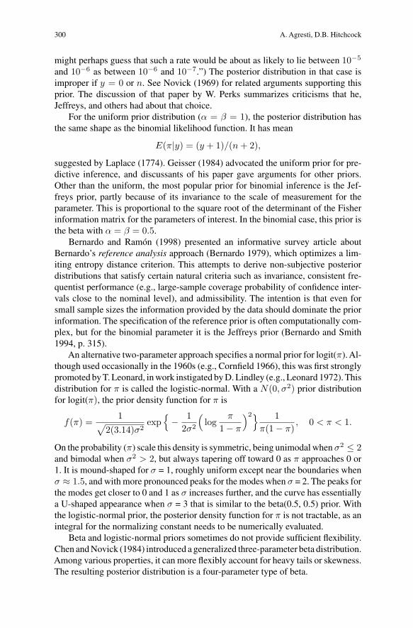
might perhaps guess that such a rate would be about as likely to lie between 10−5

and 10−6 as between 10−6 and 10−7.”) The posterior distribution in that case isimproper if y = 0 or n. See Novick (1969) for related arguments supporting thisprior. The discussion of that paper by W. Perks summarizes criticisms that he,Jeffreys, and others had about that choice.

For the uniform prior distribution (α = β = 1), the posterior distribution hasthe same shape as the binomial likelihood function. It has mean

E(π|y) = (y + 1)/(n + 2),

suggested by Laplace (1774). Geisser (1984) advocated the uniform prior for pre-dictive inference, and discussants of his paper gave arguments for other priors.Other than the uniform, the most popular prior for binomial inference is the Jef-freys prior, partly because of its invariance to the scale of measurement for theparameter. This is proportional to the square root of the determinant of the Fisherinformation matrix for the parameters of interest. In the binomial case, this prior isthe beta with α = β = 0.5.

Bernardo and Ramon (1998) presented an informative survey article aboutBernardo’s reference analysis approach (Bernardo 1979), which optimizes a lim-iting entropy distance criterion. This attempts to derive non-subjective posteriordistributions that satisfy certain natural criteria such as invariance, consistent fre-quentist performance (e.g., large-sample coverage probability of confidence inter-vals close to the nominal level), and admissibility. The intention is that even forsmall sample sizes the information provided by the data should dominate the priorinformation. The specification of the reference prior is often computationally com-plex, but for the binomial parameter it is the Jeffreys prior (Bernardo and Smith1994, p. 315).

An alternative two-parameter approach specifies a normal prior for logit(π). Al-though used occasionally in the 1960s (e.g., Cornfield 1966), this was first stronglypromoted by T. Leonard, in work instigated by D. Lindley (e.g., Leonard 1972). Thisdistribution for π is called the logistic-normal. With a N(0, σ2) prior distributionfor logit(π), the prior density function for π is

f(π) =1√

2(3.14)σ2exp

{− 1

2σ2

(log

π

1 − π

)2} 1π(1 − π)

, 0 < π < 1.

On the probability (π) scale this density is symmetric, being unimodal when σ2 ≤ 2and bimodal when σ2 > 2, but always tapering off toward 0 as π approaches 0 or1. It is mound-shaped for σ = 1, roughly uniform except near the boundaries whenσ ≈ 1.5, and with more pronounced peaks for the modes when σ = 2. The peaks forthe modes get closer to 0 and 1 as σ increases further, and the curve has essentiallya U-shaped appearance when σ = 3 that is similar to the beta(0.5, 0.5) prior. Withthe logistic-normal prior, the posterior density function for π is not tractable, as anintegral for the normalizing constant needs to be numerically evaluated.

Beta and logistic-normal priors sometimes do not provide sufficient flexibility.Chen and Novick (1984) introduced a generalized three-parameter beta distribution.Among various properties, it can more flexibly account for heavy tails or skewness.The resulting posterior distribution is a four-parameter type of beta.


2.2. Bayesian inference about a binomial parameter

Walters (1985) used the uniform prior and its implied posterior distribution in con-structing a confidence interval for a binomial parameter (in Bayesian terminology,a “credible region”). He noted how the bounds were contained in the Clopper andPearson classical ‘exact’confidence bounds based on inverting two frequentist one-sided binomial tests (e.g., the lower bound πL of a 95% Clopper-Pearson intervalsatisfies .025 = P (Y ≥ y|πL)). Brown, Cai, and DasGupta (2001, 2002) showedthat the posterior distribution generated by the Jeffreys prior yields a confidenceinterval for π with better performance in terms of average (across π) coverage prob-ability and expected length. It approximates the small-sample confidence intervalbased on inverting two binomial frequentist one-sided tests, when one uses the midP -value in place of the ordinary P -value. (The mid P -value is the null probabilityof more extreme results plus half the null probability of the observed result.) Seealso Leonard and Hsu (1999, pp. 142–144).

For a test of H0: π ≥ π0 against Ha: π < π0, a Bayesian P -value is the posteriorprobability, P (π ≥ π0|y). Routledge (1994) showed that with the Jeffreys prior andπ0 = 1/2, this approximately equals the one-sided mid P -value for the frequentistbinomial test.

Much literature about Bayesian inference for a binomial parameter deals withdecision-theoretic results. For estimating a parameter θ using estimator T with lossfunction w(θ)(T −θ)2, the Bayesian estimator is E[θw(θ)|y]/E[w(θ)|y] (Ferguson1967, p. 47). With loss function (T −π)2/[π(1−π)] and uniform prior distribution,the Bayes estimator of π is the ML estimator p = y/n. Johnson (1971) showed thatthis is an admissible estimator, for standard loss functions. Rukhin (1988) intro-duced a loss function that combines the estimation error of a statistical procedurewith a measure of its accuracy, an approach that motivates a beta prior with param-eter settings between those for the uniform and Jeffreys priors, converging to theuniform as n increases and to the Jeffreys as n decreases.

Diaconis and Freedman (1990) investigated the degree to which posterior distri-butions put relatively greater mass close to the sample proportion p as n increases.They showed that the posterior odds for an interval of fixed length centered at pis bounded below by a term of form abn with computable constants a > 0 andb > 1. They noted that Laplace considered this problem with a uniform prior in1774. Related work deals with the consistency of Bayesian estimators. Freedman(1963) showed consistency under general conditions for sampling from discretedistributions such as the multinomial. He also showed asymptotic normality ofthe posterior assuming a local smoothness assumption about the prior. For earlywork about the asymptotic normality of the posterior distribution for a binomialparameter, see von Mises (1964, Ch. VIII, Sect. C).

Draper and Guttman (1971) explored Bayesian estimation of the binomial sam-ple size n based on r independent binomial observations, each with parameters nand π. They considered both π known and unknown. The π unknown case arises incapture-recapture experiments for estimating population size n. One difficulty thereis that different models can fit the data well yet yield quite different projections.A later extensive Bayesian literature on the capture-recapture problem includes


Smith (1991), George and Robert (1992), Madigan and York (1997), and King andBrooks (2001a, 2002). Madigan and York (1997) explicitly accounted for modeluncertainty by placing a prior distribution over a discrete set of models as well asover n and the cell probabilities for the table of the capture-recapture observationsfor the repeated sampling. Fienberg, Johnson and Junker (1999) surveyed otherBayesian and classical approaches to this problem, focusing on ways to permit het-erogeneity in catchability among the subjects. Dobra and Fienberg (2001) used afully Bayesian specification of the Rasch model (discussed in Sect. 5.1) to estimatethe size of the World Wide Web.

Joseph, Wolfson, and Berger (1995) addressed sample size calculations forbinomial experiments, using criteria such as attaining a certain expected width of aconfidence interval. DasGupta and Zhang (2005) reviewed inference for binomialand multinomial parameters, with emphasis on decision-theoretic results.

2.3. Bayesian estimation of multinomial parameters

Results for the binomial with beta prior distribution generalize to the multinomialwith a Dirichlet prior (Lindley 1964, Good 1965). With c categories, suppose cellcounts (n1, . . . , nc) have a multinomial distribution with n =

∑ni and parameters

π = (π1, . . . , πc)′. Let {pi = ni/n} be the sample proportions. The likelihood isproportional to

c∏i=1

πnii .

The conjugate density is the Dirichlet, expressed in terms of gamma functions as

g(π) =Γ (

∑αi)

[∏

i Γ (αi)]

c∏i=1

παi−1i for 0 < πi < 1 all i,

∑i

πi = 1,

where {αi > 0}. Let K =∑

αi. The Dirichlet has E(πi) = αi/K and Var(πi) =αi(K −αi)/[K2(K +1)]. The posterior density is also Dirichlet, with parameters{ni + αi}, so the posterior mean is

E(πi|n1, . . . , nc) = (ni + αi)/(n + K).

Let γi = E(πi) = αi/K. This Bayesian estimator equals the weighted average

[n/(n + K)]pi + [K/(n + K)]γi,

which is the sample proportion when the prior information corresponds to K trialswith αi outcomes of type i, i = 1, . . . , c.

Good (1965) referred to K as a flattening constant, since with identical {αi}this estimate shrinks each sample proportion toward the equi-probability valueγi = 1/c. Greater flattening occurs as K increases, for fixed n. Good (1980)attributed {αi = 1} to De Morgan (1847), whose use of (ni+1)/(n+c) to estimateπi extended Laplace’s estimate to the multinomial case. Perks (1947) suggested


{αi = 1/c}, noting the coherence with the Jeffreys prior for the binomial (See alsohis discussion of Novick 1969). The Jeffreys prior sets all αi = 0.5. Lindley (1964)gave special attention to the improper case {αi = 0}, also considered by Novick(1969). The discussion of Novick (1969) shows the lack of consensus about what‘noninformative’ means.

The shrinkage form of estimator combines good characteristics of sample pro-portions and model-based estimators. Like sample proportions and unlike model-based estimators, they are consistent even when a particular model (such as equi-probability) does not hold. The weight given the sample proportion increases to 1.0as the sample size increases. Like model-based estimators and unlike sample pro-portions, the Bayes estimators smooth the data. The resulting estimators, althoughslightly biased, usually have smaller total mean squared error than the sample pro-portions. One might expect this, based on analogous results of Stein for estimatingmultivariate normal means. However, Bayesian estimators of multinomial parame-ters are not uniformly better than ML estimators for all possible parameter values.For instance, if a true cell probability equals 0, the sample proportion equals 0 withprobability one, so the sample proportion is better than any other estimator.

Hoadley (1969) examined Bayesian estimation of multinomial probabilitieswhen the population of interest is finite, of known size N . He argued that a finite-population analogue of the Dirichlet prior is a compound multinomial prior, whichleads to a translated compound multinomial posterior. Let N denote a vector ofnonnegative integers such that its i-th component Ni is the number of objects (outof N total) that are in category i, i = 1, . . . , c. If conditional on the probabilitiesand N , the cell counts have a multinomial distribution, and if the multinomialprobabilities themselves have a Dirichlet distribution indexed by parameter α suchthat αi > 0 for all i with K =

∑αi, then unconditionally N has the compound

multinomial mass function,

f(N|N ; α) =N ! Γ (K)

Γ (N + K)

c∏i=1

Γ (Ni + αi)Ni!Γ (αi)

.

This serves as a prior distribution for N. Given cell count data {ni} in a sample ofsize n, the posterior distribution of N - n is compound multinomial with N replacedby N − n and α replaced by α + n. Ericson (1969) gave a general Bayesiantreatment of the finite-population problem, including theoretical investigation ofthe compound multinomial.

For the Dirichlet distribution, one can specify the means through the choiceof {γi} and the variances through the choice of K, but then there is no free-dom to alter the correlations. As an alternative, Leonard (1973), Aitchison (1985),Goutis (1993), and Forster and Skene (1994) proposed using a multivariate normalprior distribution for multinomial logits. This induces a multivariate logistic-normaldistribution for the multinomial parameters. Specifically, if X = (X1, . . . , Xc)has a multivariate normal distribution, then π = (π1, . . . , πc) with πi =exp(Xi)/

∑cj=1 exp(Xj) has the logistic-normal distribution. This can provide

extra flexibility. For instance, when the categories are ordered and one expectssimilarity of probabilities in adjacent categories, one might use an autoregressive


form for the normal correlation matrix. Leonard (1973) suggested this approach inestimating a histogram.

Here is a summary of other Bayesian literature about the multinomial: Goodand Crook (1974) suggested a Bayes / non-Bayes compromise by using Bayesianmethods to generate criteria for frequentist significance testing, illustrating forthe test of multinomial equiprobability. An example of such a criterion is theBayes factor given by the prior odds of the null hypothesis divided by the pos-terior odds. See Good (1967) for related comments. Dickey (1983) discussednested families of distributions that generalize the Dirichlet distribution, and ar-gued that they were appropriate for contingency tables. Sedransk, Monahan, andChiu (1985) considered estimation of multinomial probabilities under the constraintπ1 ≤ ... ≤ πk ≥ πk+1 ≥ ... ≥ πc, using a truncated Dirichlet prior and possiblya prior on k if it is unknown. Delampady and Berger (1990) derived lower boundson Bayes factors in favor of the null hypothesis of a point multinomial probability,and related them to P -values in chi-squared tests. Bernardo and Ramon (1998)illustrated Bernardo’s reference analysis approach by applying it to the problemof estimating the ratio πi/πj of two multinomial parameters. The posterior distri-bution of the ratio depends on the counts in those two categories but not on theoverall sample size or the counts in other categories. This need not be true withconventional prior distributions. The posterior distribution of πi/(πi + πj) is thebeta with parameters ni +1/2 and nj +1/2, the Jeffreys posterior for the binomialparameter.

2.4. Hierarchical Bayesian estimates of multinomial parameters

Good (1965, 1967, 1976, 1980) noted that Dirichlet priors do not always providesufficient flexibility and adopted a hierarchical approach of specifying distributionsfor the Dirichlet parameters. This approach treats the {αi} in the Dirichlet prior asunknown and specifies a second-stage prior for them. Good also suggested that onecould obtain more flexibility with prior distributions by using a weighted average ofDirichlet distributions. See Albert and Gupta (1982) for later work on hierarchicalDirichlet priors.

These approaches gain greater generality at the expense of giving up the simpleconjugate Dirichlet form for the posterior. Once one departs from the conjugatecase, there are advantages of computation and of ease of more general hierarchicalstructure by using a multivariate normal prior for logits, as in Leonard’s work inthe 1970s discussed in Sect. 3 in particular contexts.

2.5. Empirical Bayesian methods

When they first consider the Bayesian approach, for many statisticians, having toselect a prior distribution is the stumbling block. Instead of choosing particular pa-rameters for a prior distribution, the empirical Bayesian approach uses the data to


determine parameter values for use in the prior distribution. This approach tradition-ally uses the prior density that maximizes the marginal probability of the observeddata, integrating out with respect to the prior distribution of the parameters.

Good (1956) may have been the first to use an empirical Bayesian approachwith contingency tables, estimating parameters in gamma and log-normal priorsfor association factors. Good (1965) used it to estimate the parameter value fora symmetric Dirichlet prior for multinomial parameters, the problem for whichhe also considered the above-mentioned hierarchical approach. Later research onempirical Bayesian estimation of multinomial parameters includes Fienberg andHolland (1973) and Leonard (1977a). Most of the empirical Bayesian literatureapplies in a context of estimating multiple parameters (such as several binomialparameters), and we will discuss it in such contexts in Sect. 3.

A disadvantage of the empirical Bayesian approach is not accounting for thesource of variability due to substituting estimates for prior parameters. It is in-creasingly preferred to use the hierarchical approach in which those parametersthemselves have a second-stage prior distribution, as mentioned in the previoussubsection.

3. Estimating cell probabilities in contingency tables

Bayesian methods for multinomial parameters apply to cell probabilities for a con-tingency table. With contingency tables, however, typically it is sensible to modelthe cell probabilities. It often does not make sense to regard the cell probabilities asexchangeable. Also, in many applications it is more natural to assume independentbinomial or multinomial samples rather than a single multinomial over the entiretable.

3.1. Estimating several binomial parameters

For several (say r) independent binomial samples, the contingency table has sizer×2. For simplicity, we denote the binomial parameters by {πi} (realizing that thisis somewhat of an abuse of notation, as we’ve just used {πi} to denote multinomialprobabilities).

Much of the early literature on estimating multiple binomial parameters used anempirical Bayesian approach. Griffin and Krutchkoff (1971) assumed an unknownprior on parameters for a sequence of binomial experiments. They expressed theBayesian estimator in a form that does not explicitly involve the prior but is in termsof marginal probabilities of events involving binomial trials. They substituted MLestimates π1, . . . , πr of these marginal probabilities into the expression for theBayesian estimator to obtain an empirical Bayesian estimator. Albert (1984) con-sidered interval estimation as well as point estimation with the empirical Bayesianapproach.

An alternative approach uses a hierarchical approach (Leonard 1972). At stage1, given µ and σ, Leonard assumed that {logit(πi)} are independent from a N(µ, σ2)distribution. At stage 2, he assumed an improper uniform prior for µ over the real


line and assumed an inverse chi-squared prior distribution for σ2. Specifically, heassumed that νλ/σ2 is independent of µ and has a chi-squared distribution with df= ν, where λ is a prior estimate of σ2 and ν is a measure of the sureness of the priorconviction. For simplicity, he used a limiting improper uniform prior for log(σ2).Integrating out µ and σ2, his two-stage approach corresponds to a multivariate tprior for {logit(πi)}. For sample proportions {pj}, the posterior mean estimate oflogit(πi) is approximately a weighted average of logit(pi) and a weighted averageof {logit(pj)}.

Berry and Christensen (1979) took the prior distribution of {πi} to be a Dirichletprocess prior (Ferguson 1973). With r = 2, one form of this is a measure on theunit square that is a weighted average of a product of two beta densities and a betadensity concentrated on the line where π1 = π2. The posterior is a mixture ofDirichlet processes. When r > 2 or 3, calculations were complex and numericalapproximations were given and compared to empirical Bayesian estimators.

Albert and Gupta (1983a) used a hierarchical approach with independentbeta(α, K −α) priors on the binomial parameters {πi} for which the second-stageprior had discrete uniform form,

π(α) = 1/(K − 1), α = 1, . . . , K − 1,

with K user-specified. In the resulting marginal prior for {πi}, the size of Kdetermines the extent of correlation among {πi}.Albert and Gupta (1985) suggesteda related hierarchical approach in which α has a noninformative second-stage prior.

Consonni and Veronese (1995) considered examples in which prior informa-tion exists about the way various binomial experiments cluster. They assumedexchangeability within certain subsets according to some partition, and allowedfor uncertainty about the partition using a prior over several possible partitions.Conditionally on a given partition, beta priors were used for {πi}, incorporatinghyperparameters.

Crowder and Sweeting (1989) considered a sequential binomial experiment inwhich a trial is performed with success probability π(1) and then, if a success isobserved, a second-stage trial is undertaken with success probability π(2). Theyshowed the resulting likelihood can be factored into two binomial densities, andhence termed it a bivariate binomial. They derived a conjugate prior that has certainsymmetry properties and reflects independence of π(1) and π(2).

Here is a brief summary of other work with multiple binomial parameters:Bratcher and Bland (1975) extended Bayesian decision rules for multiple compar-isons of means of normal populations to the problem of ordering several binomialprobabilities, using beta priors. Sobel (1993) presented Bayesian and empiricalBayesian methods for ranking binomial parameters, with hyperparameters esti-mated either to maximize the marginal likelihood or to minimize a posterior riskfunction. Springer and Thompson (1966) derived the posterior distribution of theproduct of several binomial parameters (which has relevance in reliability con-texts) based on beta priors. Franck et al. (1988) considered estimating posteriorprobabilities about the ratio π2/π1 for an application in which it was appropriate totruncate beta priors to place support over π2 ≤ π1. Sivaganesan and Berger (1993)


used a nonparametric empirical Bayesian approach assuming that a set of binomialparameters come from a completely unknown prior distribution.

3.2. Estimating multinomial cell probabilities

Next, we consider arbitrary-size contingency tables, under a single multinomialsample. The notation will refer to two-way r × c tables with cell counts n = {nij}and probabilities π = {πij}, but the ideas extend to any dimension.

Fienberg and Holland (1972, 1973) proposed estimates of {πij} using data-dependent priors. For a particular choice of Dirichlet means {γij} for the Bayesianestimator

[n/(n + K)]pij + [K/(n + K)]γij ,

they showed that the minimum total mean squared error occurs when

K =(1 −

∑π2

ij

)/

[∑(γij − πij)2

].

The optimal K = K(γ,π) depends on π, and they used the estimate K(γ,p).As pfalls closer to the prior guess γ, K(γ,p) increases and the prior guess receives moreweight in the posterior estimate. They selected {γij} based on the fit of a simplemodel. For two-way tables, they used the independence fit {γij = pi+p+j} for thesample marginal proportions. For extensions and further elaboration, see Chapter12 of Bishop, Fienberg, and Holland (1975). When the categories are ordered,improved performance usually results from using the fit of an ordinal model, suchas the linear-by-linear association model (Agresti and Chuang 1989).

Epstein and Fienberg (1992) suggested two-stage priors on the cell probabilities,first placing a Dirichlet(K, γ)prior onπ and using a loglinear parametrization of theprior means {γij}. The second stage places a multivariate normal prior distributionon the terms in the loglinear model for {γij}.Applying the loglinear parametrizationto the prior means {γij} rather than directly to the cell probabilities {πij} permitsthe analysis to reflect uncertainty about the loglinear structure for {πij}. This wasone of the first uses of Gibbs sampling to calculate posterior densities for cellprobabilities.

Albert and Gupta wrote several articles in the early 1980s exploring Bayesianestimation for contingency tables. Albert and Gupta (1982) used hierarchicalDirichlet(K, γ) priors for π for which {γij} reflect a prior belief that the prob-abilities may be either symmetric or independent. The second stage places a non-informative uniform prior on γ. The precision parameter K reflects the strength ofprior belief, with large K indicating strong belief in symmetry or independence.Albert and Gupta (1983a) considered 2×2 tables in which the prior informationwas stated in terms of either the correlation coefficient ρ between the two variablesor the odds ratio (π11π22/π12π21). Albert and Gupta (1983b) used a Dirichlet prioron {πij}, but instead of a second-stage prior, they reparametrized so that the prioris determined entirely by the prior guesses for the odds ratio and K. They showed


how to make a prior guess for K by specifying an interval covering the middle 90%of the prior distribution of the odds ratio.

Albert (1987b) discussed derivations of the estimator of form (1−λ)pij +λπij ,where πij = pi+p+j is the independence estimate and λ is some function of thecell counts. The conjugate Bayesian multinomial estimator of Fienberg and Holland(1973) shown above has such a form, as do estimators of Leonard (1975) and Laird(1978). Albert (1987b) extended Albert and Gupta (1982, 1983b) by suggestingempirical Bayesian estimators that use mixture priors. For cell counts n = {nij},Albert derived approximate posterior moments

E(πij |n, K) ≈ (nij + Kpi+p+j)/(n + K)

that have the form (1−λ)pij +λπij . He suggested estimating K from the marginaldensity m(n|K) and plugging in the estimate to obtain an empirical Bayesianestimate. Alternatively, a hierarchical Bayesian approach places a noninformativeprior on K and uses the resulting posterior estimate of K.

3.3. Estimating loglinear model parameters in two-way tables

The Bayesian approaches presented so far focused directly on estimating probabil-ities, with prior distributions specified in terms of them. One could instead focuson association parameters. Lindley (1964) did this with r × c contingency tables,using a Dirichlet prior distribution (and its limiting improper prior) for the multi-nomial. He showed that contrasts of log cell probabilities, such as the log oddsratio, have an approximate (large-sample) joint normal posterior distribution. Thisgives Bayesian analogs of the standard frequentist results for two-way contingencytables. Using the same structure as Lindley (1964), Bloch and Watson (1967) pro-vided improved approximations to the posterior distribution and also consideredlinear combinations of the cell probabilities.

As mentioned previously, a disadvantage of a one-stage Dirichlet prior is that itdoes not allow for placing structure on the probabilities, such as corresponding toa loglinear model. Leonard (1975), based on his thesis work, considered loglinearmodels, focusing on parameters of the saturated model

log[E(nij)] = λ + λXi + λY

j + λXYij

using normal priors. Leonard argued that exchangeability within each set of log-linear parameters is more sensible than the exchangeability of multinomial proba-bilities that one gets with a Dirichlet prior. He assumed that the row effects {λX

i },column effects {λY

j }, and interaction effects {λXYij } were a priori independent.

For each of these three sets, given a mean µ and variance σ2, the first-stage priortakes them to be independent and N(µ, σ2). As in Leonard’s 1972 work for severalbinomials, at the second stage each normal mean is assumed to have an improperuniform distribution over the real line, and σ2 is assumed to have an inverse chi-squared distribution. For computational convenience, parameters were estimatedby joint posterior modes rather than posterior means. The analysis shrinks the logcounts toward the fit of the independence model.


Laird (1978), building on Good (1956) and Leonard (1975), estimated cell prob-abilities using an empirical Bayesian approach with the loglinear model. Her basicmodel differs somewhat from Leonard’s (1975). She assumed improper uniformpriors over the real line for the main effect parameters and independent N(0, σ2)distributions for the interaction parameters. For computational convenience, as inLeonard (1975) the loglinear parameters were estimated by their posterior modes,and those posterior modes were plugged into the loglinear formula to get cell prob-ability estimates. The empirical Bayesian aspect occurs from replacing σ2 by themode of the marginal likelihood, after integrating out the loglinear parameters. Asσ → ∞, the estimates converge to the sample proportions; as σ → 0, they convergeto the independence estimates, {pi+p+j}. The fitted values have the same row andcolumn marginal totals as the observed data. She noted that the use of a symmetricDirichlet prior results in estimates that correspond to adding the same count to eachcell, whereas her approach permits considerable variability in the amount added orsubtracted from each cell to get the fitted value.

In related work, Jansen and Snijders (1991) considered the independence modeland used lognormal or gamma priors for the parameters in the multiplicative form ofthe model, noting the better computational tractability of the gamma approach. Moregenerally, Albert (1988) used a hierarchical approach for estimating a loglinearPoisson regression model, assuming a gamma prior for the Poisson means and anoninformative prior on the gamma parameters.

Square contingency tables with the same categories for rows and columns haveextra structure that can be recognized through models that are permutation invari-ant for certain groups of transformations of the cells. Forster (2004b) consideredsuch models and discussed how to construct invariant prior distributions for themodel parameters. As mentioned previously, Albert and Gupta (1982) had useda hierarchical Dirichlet approach to smoothing toward a prior belief of symmetry.Vounatsou and Smith (1996) analyzed certain structured contingency tables, includ-ing symmetry, quasi-symmetry and quasi-independence models for square tablesand for triangular tables that result when the category corresponding to the (i, j)cell is indistinguishable from that of the (j, i) cell (a case also studied by Altham1975). They assessed goodness of fit using distance measures and by comparingsample predictive distributions of counts to corresponding observed values.

Here is a summary of some other Bayesian work on loglinear-related modelsfor two-way tables. Leighty and Johnson (1990) used a two-stage procedure thatfirst locates full and reduced loglinear models whose parameter vectors enclosethe important parameters and then uses posterior regions to identify which onesare important. Evans, Gilula, and Guttman (1993) provided a Bayesian analysis ofGoodman’s generalization of the independence model that has multiplicative rowand column effects, called the RC model. Kateri, Nicolaou, and Ntzoufras (2005)considered Goodman’s more general RC(m) model. Evans, Gilula, and Guttman(1989) noted that latent class analysis in two-way tables usually encounters identi-fiability conditions, which can be overcome with a Bayesian approach putting priordistributions on the latent parameters.


3.4. Extensions to multi-dimensional tables

Knuiman and Speed (1988) generalized Leonard’s loglinear modeling approach byconsidering multi-way tables and by taking a multivariate normal prior for all pa-rameters collectively rather than univariate normal priors on individual parameters.They noted that this permits separate specification of prior information for differentinteraction terms, and they applied this to unsaturated models. They computed theposterior mode and used the curvature of the log posterior at the mode to measureprecision. King and Brooks (2001b) also specified a multivariate normal prior onthe loglinear parameters, which induces a multivariate log-normal prior on the ex-pected cell counts. They derived the parameters of this distribution in an explicitform and stated the corresponding mean and covariances of the cell counts.

For frequentist methods, it is well known that one can analyze a multinomialloglinear model using a corresponding Poisson loglinear model (before condition-ing on the sample size), in order to avoid awkward constraints. Following Knuimanand Speed (1988), Forster (2004a) considered corresponding Bayesian results, alsousing a multivariate normal prior on the model parameters. He adopted prior spec-ification having invariance under certain permutations of cells (e.g., not alteringstrata). Under such restrictions, he discussed conditions for prior distributions suchthat marginal inferences are equivalent for Poisson and multinomial models. Theseessentially allow the parameter governing the overall size of the cell means (whichdisappears after the conditioning that yields the multinomial model) to have animproper prior. Forster also derived necessary and sufficient conditions for the pos-terior to then be proper, and he related them to conditions for maximum likelihoodestimates to be finite. An advantage of the Poisson parameterization is that Markovchain Monte Carlo (MCMC) methods are typically more straightforward to ap-ply than with multinomial models. (See Sect. 6 for a brief discussion of MCMCmethods.)

Loglinear model selection, particularly using Bayes factors, now has a substan-tial literature. Spiegelhalter and Smith (1982) gave an approximate expression forthe Bayes factor for a multinomial loglinear model with an improper prior (uni-form for the log probabilities) and showed how it related to the standard chi-squaredgoodness-of-fit statistic. Raftery (1986) noted that this approximation is indeter-minate if any cell is empty but is valid with a Jeffreys prior. He also noted that,with large samples, -2 times the log of this approximate Bayes factor is approx-imately equivalent to Schwarz’s BIC model selection criterion. More generally,Raftery (1996) used the Laplace approximation to integration to obtain approx-imate Bayes factors for generalized linear models. Madigan and Raftery (1994)proposed a strategy for loglinear model selection with Bayes factors that employsmodel averaging. See also Raftery (1996) and Dellaportas and Forster (1999) forrelated work. Albert (1996) suggested partitioning the loglinear model parametersinto subsets and testing whether specific subsets are nonzero. Using normal priorsfor the parameters, he examined the behavior of the Bayes factor under both normaland Cauchy priors, finding that the Cauchy was more robust to misspecified priorbeliefs. Ntzoufras, Forster and Dellaportas (2000) developed a MCMC algorithmfor loglinear model selection.


An interesting recent application of Bayesian loglinear modeling is to issuesof confidentiality (Fienberg and Makov 1998). Agencies often release multidimen-sional contingency tables that are ostensibly confidential, but the confidentialitycan be broken if an individual is uniquely identifiable from the data presentation.Fienberg and Makov considered loglinear modeling of such data, accounting formodel uncertainty via Bayesian model averaging.

Considerable literature has dealt with analyzing a set of 2 × 2 contingency ta-bles, such as often occur in meta analyses or multi-center clinical trials comparingtwo treatments on a binary response. Maritz (1989) derived empirical Bayesianestimators for the log-odds ratios, based on a Dirichlet prior for the cell proba-bilities and estimating the hyperparameters using data from the other tables. SeeAlbert (1987a) for related work. Wypij and Santner (1992) considered the modelof a common odds ratio and used Bayesian and empirical Bayesian arguments tomotivate an estimator that corresponds to a conditional ML estimator after adding acertain number of pseudotables that have a concordant or discordant pair of obser-vations. Skene and Wakefield (1990) modeled multi-center studies using a modelthat allows the treatment–response log odds ratio to vary among centers. Meng andDempster (1987) considered a similar model, using normal priors for main effectand interaction parameters in a logit model, in the context of dealing with the mul-tiplicity problem in hypothesis testing with many 2×2 tables. Warn, Thompson,and Spiegelhalter (2002) considered meta analyses for the difference and the ratioof proportions. This relates essentially to identity and log link analogs of the logitmodel, in which case it is necessary to truncate normal prior distributions so thedistributions apply to the appropriate set of values for these measures. Efron (1996)outlined empirical Bayesian methods for estimating parameters corresponding tomany related populations, exemplified by odds ratios from 41 different trials ofa surgical treatment for ulcers. His method permits selection from a wide classof priors in the exponential family. Casella (2001) analyzed data from Efron’smeta-analysis, estimating the hyperparameters as in an empirical Bayes analysisbut using Gibbs sampling to approximate the posterior of the hyperparameters,thereby gaining insight into the variability of the hyperparameter terms. Casellaand Moreno (2005) gave another approach to the meta-analysis of contingencytables, employing intrinsic priors. Wakefield (2004) discussed the sensitivity ofvarious hierarchical approaches for ecological inference, which involves makinginferences about the associations in the separate 2×2 tables when one observesonly the marginal distributions.

3.5. Graphical models

Much attention has been paid in recent years to graphical models. These havecertain conditional independence structure that is easily summarized by a graphwith vertices for the variables and edges between vertices to represent a condi-tional association. The cell probabilities can be expressed in terms of marginal andconditional probabilities, and independent Dirichlet prior distributions for them in-duce independent Dirichlet posterior distributions. See O’Hagan and Forster (2004,


Ch. 12) for discussion of the usefulness of graphical representations for a varietyof Bayesian analyses.

Dawid and Lauritzen (1993) introduced the notion of a probability distributiondefined over probability measures on a multivariate space that concentrate on a set ofsuch graphs. A special case includes a hyper Dirichlet distribution that is conjugatefor multinomial sampling and that implies that certain marginal probabilities havea Dirichlet distribution. Madigan and Raftery (1994) and Madigan andYork (1995)used this family for graphical model comparison and for constructing posteriordistributions for measures of interest by averaging over relevant models. Giudici(1998) used a prior distribution over a space of graphical models to smooth cellcounts in sparse contingency tables, comparing his approach with the simple onebased on a Dirichlet prior for multinomial probabilities.

3.6. Dealing with nonresponse

Several authors have considered Bayesian approaches in the presence of nonre-sponse. Modeling nonignorable nonresponse has mainly taken one of two ap-proaches: Introducing parameters that control the extent of nonignorability intothe model for the observed data and checking the sensitivity to these parameters,or modeling of the joint distribution of the data and the response indicator. Forsterand Smith (1998) reviewed these approaches and cited relevant literature.

Forster and Smith (1998) considered models having categorical response andcategorical covariate vector, when some response values are missing. They in-vestigated a Bayesian method for selecting between nonignorable and ignorablenonresponse models, pointing out that the limited amount of information availablemakes standard model comparison methods inappropriate. Other works dealingwith missing data for categorical responses include Basu and Pereira (1982), Al-bert and Gupta (1985), Kadane (1985), Dickey, Jiang, and Kadane (1987), Park andBrown (1994), Paulino and Pereira (1995), Park (1998), Bradlow and Zaslavsky(1999), and Soares and Paulino (2001). Viana (1994) and Prescott and Garthwaite(2002) studied misclassified multinomial and binary data, respectively, with appli-cations to misclassified case-control data.

4. Tests and confidence intervals in two-way tables

We next consider Bayesian analogs of frequentist significance tests and confidenceintervals for contingency tables. For 2×2 tables, with multinomial Dirichlet priorsor binomial beta priors there are connections between Bayesian and frequentistresults.

4.1. Confidence intervals for association parameters

For 2× 2 tables resulting from two independent binomial samples with parametersπ1 and π2, the measures of usual interest are π1 − π2, the relative risk π1/π2, and


the odds ratio [π1/(1−π1)]/[π2/(1−π2)]. It is most common to use a beta(αi, βi)prior for πi, i = 1, 2, taking them to be independent. Alternatively, one could usea correlated prior. An obvious possibility is the bivariate normal for [logit(π1),logit(π2)]. Howard (1998) instead amended the independent beta priors and usedprior density function proportional to

e−(1/2)u2πa−1

1 (1 − π1)b−1πc−12 (1 − π2)d−1,

where

u =1σ

log(

π1(1 − π2)π2(1 − π1)

).

Howard suggested σ = 1 for a standard form.The priors forπ1 andπ2 induce corresponding priors for the measures of interest.

For instance, with uniform priors, π1−π2 has a symmetrical triangular density over(-1, +1), r = π1/π2 has density g(r) = 1/2 for 0 ≤ r ≤ 1 and g(r) = 1/(2r2)for r > 1, and the log odds ratio has the Laplace density (Nurminen and Mutanen1987). The posterior distribution for (π1, π2) induces posterior distributions for themeasures. For the independent beta priors, Hashemi, Nandram and Goldberg (1997)and Nurminen and Mutanen (1987) gave integral expressions for the posteriordistributions for the difference, ratio, and odds ratio.

Hashemi et al. (1997) formed Bayesian highest posterior density (HPD) con-fidence intervals for these three measures. With the HPD approach, the posteriorprobability equals the desired confidence level and the posterior density is higherfor every value inside the interval than for every value outside of it. The HPD in-terval lacks invariance under parameter transformation. This is a serious liabilityfor the odds ratio and relative risk, unless the HPD interval is computed on the logscale. For instance, if (L, U) is a 100(1 − α)% HPD interval using the posteriordistribution of the odds ratio, then the 100(1 − α)% HPD interval using the pos-terior distribution of the inverse of the odds ratio (which is relevant if we reversethe identification of the two groups being compared) is not (1/U, 1/L). The “tailmethod” 100(1 − α)% interval consists of values between the α/2 and (1 − α/2)quantiles. Although longer than the HPD interval, it is invariant.

Agresti and Min (2005) discussed Bayesian confidence intervals for associ-ation parameters in 2×2 tables. They argued that if one desires good coverageperformance (in the frequentist sense) over the entire parameter space, it is best touse quite diffuse priors. Even uniform priors are often too informative, and theyrecommended the Jeffreys prior.

4.2. Tests comparing two independent binomial samples

Using independent beta priors, Novick and Grizzle (1965) focused on finding theposterior probability that π1 > π2 and discussed application to sequential clinicaltrials. Cornfield (1966) also examined sequential trials from a Bayesian viewpoint,focusing on stopping-rule theory. He used prior densities that concentrate somenonzero probability at the null hypothesis point. His test assumed normal priors for


µi = logit(πi), i = 1, 2, putting a nonzero prior probability λ on the null µ1 = µ2.From this, Cornfield derived the posterior probability that µ1 = µ2 and showedconnections with stopping-rule theory.

Altham (1969) discussed Bayesian testing for 2×2 tables in a multinomialcontext. She treated the cell probabilities {πij} as multinomial parameters havinga Dirichlet prior with parameters {αij}. For testing H0: θ = π11π22/π12π21 ≤ 1against Ha: θ > 1 with cell counts {nij} and the posterior Dirichlet distributionwith parameters {α

′ij = αij + nij}, she showed that

P (θ ≤ 1|{nij}) =α

′21−1∑

s=max(α′21−α

′12,0)

(α

′+1 − 1

s

)(α

′+2 − 1

α′2+ − 1 − s

)/

(α

′++ − 2

α′1+ − 1

).

This posterior probability equals the one-sided P-value for Fisher’s exact test, whenone uses the improper prior hyperparameters α11 = α22 = 0 and α12 = α21 =1, which correspond to a prior belief favoring the null hypothesis. That is, theordinary P -value for Fisher’s exact test corresponds to a Bayesian P -value with aconservative prior distribution, which some have taken to reflect the conservativenature of Fisher’s exact test. If αij = γ, i, j = 1, 2, with 0 ≤ γ ≤ 1, Althamshowed that the Bayesian P -value is smaller than the Fisher P -value. The differencebetween the two is no greater than the null probability of the observed data.

Altham’s results extend to comparing independent binomials with correspond-ing beta priors. In that case, see Irony and Pereira (1986) for related work comparingFisher’s exact test with a Bayesian test. See Seneta (1994) for discussion of anotherhypergeometric test having a Bayesian-type derivation, due to Carl Liebermeisterin 1877, that can be viewed as a forerunner of Fisher’s exact test. Howard (1998)showed that with Jeffreys priors the posterior probability that π1 ≤ π2 approxi-mates the one-sided P -value for the large-sample z test using pooled variance (i.e.,the signed square root of the Pearson statistic) for testing H0 : π1 = π2 againstHa : π1 > π2.

Little (1989) argued that if one believes in conditioning on approximate an-cillary statistics, then the conditional approach leads naturally to the likelihoodprinciple and to a Bayesian analysis such as Altham’s. Zelen and Parker (1986)considered Bayesian analyses for 2×2 tables that result from case-control studies.They argued that the Bayesian approach is well suited for this, since such studiesdo not represent randomized experiments or random samples from a real or hypo-thetical population of possible experiments. Later Bayesian work on case-controlstudies includes Ghosh and Chen (2002), Muller and Roeder (1997), Seaman andRichardson (2004), and Sinha, Mukherjee, and Ghosh (2004). For instance, Sea-man and Richardson (2004) extend to Bayesian methods the equivalence betweenprospective and retrospective models in case-control studies. See Berry (2004) fora recent exposition of advantages of using a Bayesian approach in clinical trials.

Weisberg (1972) extended Novick and Grizzle (1965) and Altham (1969) to thecomparison of two multinomial distributions with ordered categories. Assumingindependent Dirichlet priors, he obtained an expression for the posterior probabilitythat one distribution is stochastically larger than the other. In the binary case, healso obtained the posterior distribution of the relative risk.


Kass and Vaidyanathan (1992) studied sensitivity of Bayes factors to smallchanges in prior distributions. Under a certain null orthogonality of the parameter ofinterest and the nuisance parameter, and with the two parameters being independenta priori, they showed that small alterations in the prior for the nuisance parameterhave no effect on the Bayes factor up to order n−1. They illustrated this for testingequality of binomial parameters.

Walley, Gurrin, and Burton (1996) suggested using a large class of prior dis-tributions to generate upper and lower probabilities for testing a hypothesis. Theseare obtained by maximizing and minimizing the probability with respect to thedensity functions in that class. They applied their approach to clinical trials datafor deciding which of two therapies is better. See also Walley (1996) for discussionof a related “imprecise Dirichlet model” for multinomial data.

Brooks (1987) used a Bayesian approach for the design problem of choosing theratio of sample sizes for comparing two binomial proportions. Matthews (1999) alsoconsidered design issues in the context of two-sample comparisons. In that simplesetting, he presented the optimal Bayesian design for estimation of the log oddsratio, and he also studied the effect of the specification of the prior distributions.

4.3. Testing independence in two-way tables

Gunel and Dickey (1974) considered independence in two-way contingency ta-bles under the Poisson, multinomial, independent multinomial, and hypergeometricsampling models. Conjugate gamma priors for the Poisson model induce priors ineach further conditioned model. They showed that the Bayes factor for indepen-dence itself factorizes, highlighting the evidence residing in the marginal totals.

Good (1976) also examined tests of independence in two-way tables based onthe Bayes factor, as did Jeffreys for 2×2 tables in later editions of his book. As insome of his earlier work, for a prior distribution Good used a mixture of symmetricDirichlet distributions. Crook and Good (1980) developed a quantitative measureof the amount of evidence about independence provided by the marginal totals anddiscussed conditions under which this is small. See also Crook and Good (1982)and Good and Crook (1987).

Albert (1997) generalized Bayesian methods for testing independence and es-timating odds ratios to other settings, extending Albert (1996). He used a priordistribution for the loglinear association parameters that reflects a belief that onlypart of the table reflects independence (a “quasi-independence” prior model) or thatthere are a few “deviant cells,” without knowing where these outlying cells are inthe table. Quintana (1998) proposed a nonparametric Bayesian analysis for devel-oping a Bayes factor to assess homogeneity of several multinomial distributions,using Dirichlet process priors. The model has the flexibility of assuming no specificform for the distribution of the multinomial probabilities.

Intrinsic priors, introduced for model selection and hypothesis testing by Bergerand Pericchi (1996), allow a conversion of an improper noninformative prior intoa proper one. For testing independence in contingency tables, Casella and Moreno(2002), noting that many common noninformative priors cannot be centered at thenull hypothesis, suggested the use of intrinsic priors.


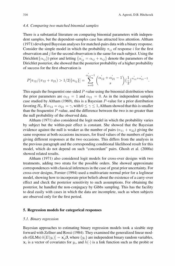
4.4. Comparing two matched binomial samples

There is a substantial literature on comparing binomial parameters with indepen-dent samples, but the dependent-samples case has attracted less attention. Altham(1971) developed Bayesian analyses for matched-pairs data with a binary response.Consider the simple model in which the probability πij of response i for the firstobservation and j for the second observation is the same for each subject. Using theDirichlet({αij}) prior and letting {α

′ij = αij + nij} denote the parameters of the

Dirichlet posterior, she showed that the posterior probability of a higher probabilityof success for the first observation is

P [π12/(π12 + π21) > 1/2|{nij}] =α

′12−1∑s=0

(α

′12 + α

′21 − 1

s

)(12)α

′12+α

′21−1

.

This equals the frequentist one-sided P -value using the binomial distribution whenthe prior parameters are α12 = 1 and α21 = 0. As in the independent samplescase studied by Altham (1969), this is a Bayesian P -value for a prior distributionfavoring H0. If α12 = α21 = γ, with 0 ≤ γ ≤ 1,Altham showed that this is smallerthan the frequentist P -value, and the difference between the two is no greater thanthe null probability of the observed data.

Altham (1971) also considered the logit model in which the probability variesby subject but the within-pair effect is constant. She showed that the Bayesianevidence against the null is weaker as the number of pairs (n11 + n22) giving thesame response at both occasions increases, for fixed values of the numbers of pairsgiving different responses at the two occasions. This differs from the analysis inthe previous paragraph and the corresponding conditional likelihood result for thismodel, which do not depend on such “concordant” pairs. Ghosh et al. (2000a)showed related results.

Altham (1971) also considered logit models for cross-over designs with twotreatments, adding two strata for the possible orders. She showed approximatecorrespondences with classical inferences in the case of great prior uncertainty. Forcross-over designs, Forster (1994) used a multivariate normal prior for a loglinearmodel, showing how to incorporate prior beliefs about the existence of a carry-overeffect and check the posterior sensitivity to such assumptions. For obtaining theposterior, he handled the non-conjugacy by Gibbs sampling. This has the facilityto deal easily with cases in which the data are incomplete, such as when subjectsare observed only for the first period.

5. Regression models for categorical responses

5.1. Binary regression

Bayesian approaches to estimating binary regression models took a sizable stepforward with Zellner and Rossi (1984). They examined the generalized linear mod-els (GLMs) h[E(yi)] = x

′iβ, where {yi} are independent binary random variables,

xi is a vector of covariates for yi, and h(·) is a link function such as the probit or


logit. They derived approximate posterior densities both for an improper uniformprior on β and for a general class of informative priors, giving particular attentionto the multivariate normal. Their approach is discussed further in Sect. 6.

Ibrahim and Laud (1991) considered the Jeffreys prior for β in a GLM, giv-ing special attention to its use with logistic regression. They showed that it is aproper prior and that all joint moments are finite, as is also true for the posteriordistribution. See also Poirier (1994). Wong and Mason (1985) extended logisticregression modeling to a multilevel form of model. Daniels and Gatsonis (1999)used such modeling to analyze geographic and temporal trends with clustered lon-gitudinal binary data. Biggeri, Dreassi, and Marchi (2004) used it to investigate thejoint contribution of individual and aggregate (population-based) socioeconomicfactors to mortality in Florence. They illustrated how an individual-level analysisthat ignored the multilevel structure could produce biased results.

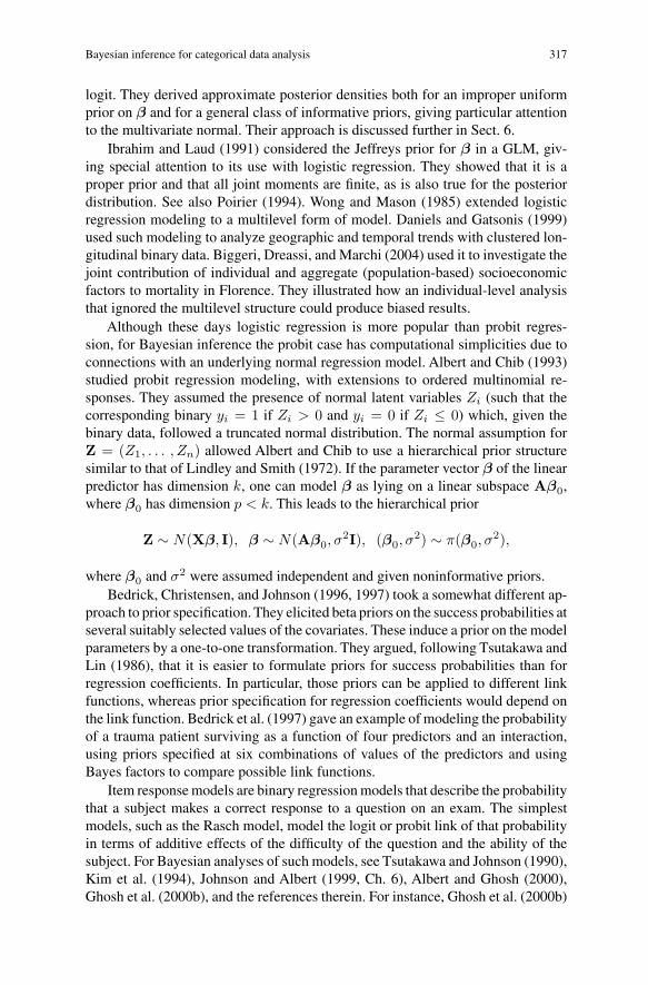
Although these days logistic regression is more popular than probit regres-sion, for Bayesian inference the probit case has computational simplicities due toconnections with an underlying normal regression model. Albert and Chib (1993)studied probit regression modeling, with extensions to ordered multinomial re-sponses. They assumed the presence of normal latent variables Zi (such that thecorresponding binary yi = 1 if Zi > 0 and yi = 0 if Zi ≤ 0) which, given thebinary data, followed a truncated normal distribution. The normal assumption forZ = (Z1, . . . , Zn) allowed Albert and Chib to use a hierarchical prior structuresimilar to that of Lindley and Smith (1972). If the parameter vector β of the linearpredictor has dimension k, one can model β as lying on a linear subspace Aβ0,where β0 has dimension p < k. This leads to the hierarchical prior

Z ∼ N(Xβ, I), β ∼ N(Aβ0, σ2I), (β0, σ

2) ∼ π(β0, σ2),

where β0 and σ2 were assumed independent and given noninformative priors.Bedrick, Christensen, and Johnson (1996, 1997) took a somewhat different ap-

proach to prior specification. They elicited beta priors on the success probabilities atseveral suitably selected values of the covariates. These induce a prior on the modelparameters by a one-to-one transformation. They argued, following Tsutakawa andLin (1986), that it is easier to formulate priors for success probabilities than forregression coefficients. In particular, those priors can be applied to different linkfunctions, whereas prior specification for regression coefficients would depend onthe link function. Bedrick et al. (1997) gave an example of modeling the probabilityof a trauma patient surviving as a function of four predictors and an interaction,using priors specified at six combinations of values of the predictors and usingBayes factors to compare possible link functions.

Item response models are binary regression models that describe the probabilitythat a subject makes a correct response to a question on an exam. The simplestmodels, such as the Rasch model, model the logit or probit link of that probabilityin terms of additive effects of the difficulty of the question and the ability of thesubject. For Bayesian analyses of such models, see Tsutakawa and Johnson (1990),Kim et al. (1994), Johnson and Albert (1999, Ch. 6), Albert and Ghosh (2000),Ghosh et al. (2000b), and the references therein. For instance, Ghosh et al. (2000b)


considered necessary and conditions for posterior distributions to be proper whenpriors are improper.

Another important application of logistic regression is in modeling trend, suchas in developmental toxicity experiments. Dominici and Parmigiani (2001) pro-posed a Bayesian semiparametric analysis that combines parametric dose-responserelationships with a flexible nonparametric specification of the distribution of the re-sponse, obtained using a Dirichlet process mixture approach. The degree to whichthe distribution of the response adapts nonparametrically to the observations isdriven by the data, and the marginal posterior distribution of the parameters of in-terest has closed form. Special cases include ordinary logistic regression, the beta-binomial model, and finite mixture models. Dempster, Selwyn, and Weeks (1983)and Ibrahim, Ryan, and Chen (1998) discussed the use of historical controls to ad-just for covariates in trend tests for binary data. Extreme versions include logisticregression either completely pooling or completely ignoring historical controls.

Greenland (2001) argued that for Bayesian implementation of logistic and Pois-son models with large samples, both the prior and the likelihood can be approxi-mated with multivariate normals, but with sparse data, such approximations may beinadequate. For sparse data, he recommended exact conjugate analysis. Giving con-jugate priors for the coefficient vector in logistic and Poisson models, he introduceda computationally feasible method of augmenting the data with binomial “pseudo-data” having an appropriate prior mean and variance. Greenland also discussed theadvantages conjugate priors have over noninformative priors in epidemiologicalstudies, showing that flat priors on regression coefficients often imply ridiculousassumptions about the effects of the clinical variables.

Piegorsch and Casella (1996) discussed empirical Bayesian methods for lo-gistic regression and the wider class of GLMs, through a hierarchical approach.They also suggested an extension of the link function through the inclusion of ahyperparameter. All the hyperparameters were estimated via marginal maximumlikelihood.

Here is a summary of other literature involving Bayesian binary regression mod-eling. Hsu and Leonard (1997) proposed a hierarchical approach that smoothes thedata in the direction of a particular logistic regression model but does not require es-timates to perfectly satisfy that model. Chen, Ibrahim, andYiannoutsos (1999) con-sidered prior elicitation and variable selection in logistic regression. Chaloner andLarntz (1989) considered determination of optimal design for experiments usinglogistic regression. Zocchi and Atkinson (1999) considered design for multinomiallogistic models. Dey, Ghosh, and Mallick (2000) edited a collection of articles thatprovided Bayesian analyses for GLMs. In that volume Gelfand and Ghosh (2000)surveyed the subject and Chib (2000) modeled correlated binary data.

5.2. Multi-category responses

For frequentist inference with a multinomial response variable, popular models in-clude logit and probit models for cumulative probabilities when the response is ordi-nal (such as logit[P (yi ≤ j)] = αj +x

′iβ), and multinomial logit and probit models


when the response is nominal (such as log[P (yi = j)/P (yi = c)] = αj + x′iβj).

The ordinal models can be motivated by underlying logistic or normal latent vari-ables. Johnson and Albert (1999) focused on ordinal models. Specification of priorsis not simple, and they used an approach that specifies beta prior distributions forthe cumulative probabilities at several values of the explanatory variables (e.g.,see p. 133). They fitted the model using a hybrid Metropolis-Hastings/Gibbs sam-pler that recognizes an ordering constraint on the {αj}. Among special cases, theyconsidered an ordinal extension of the item response model.

Chipman and Hamada (1996) used the cumulative probit model but with anormal prior defined directly on β and a truncated ordered normal prior for the{αj}, implementing it with the Gibbs sampler. For binary and ordinal regression,Lang (1999) used a parametric link function based on smooth mixtures of twoextreme value distributions and a logistic distribution. His model used a flat, non-informative prior for the regression parameters, and was designed for applicationsin which there is some prior information about the appropriate link function.

Bayesian ordinal models have been used for various applications. For instance,Chipman and Hamada (1996) analyzed two industrial data sets. Johnson (1996)proposed a Bayesian model for agreement in which several judges provide ordinalratings of items, a particular application being test grading. Johnson assumed thatfor a given item, a normal latent variable underlies the categorical rating. The modelis used to regress the latent variables for the items on covariates in order to comparethe performance of raters. Broemeling (2001) employed a multinomial-Dirichletsetup to model agreement among multiple raters. For other Bayesian analyses withordinal data, see Bradlow and Zaslavsky (1999), Ishwaran and Gatsonis (2000),and Rossi, Gilula, and Allenby (2001).

For nominal responses, Daniels and Gatsonis (1997) used multinomial logitmodels to analyze variations in the utilization of alternative cardiac proceduresin a study of Medicare patients who had suffered myocardial infarction. Theirmodel generalized the Wong and Mason (1985) hierarchical approach. They useda multivariate t distribution for the regression parameters, with vague proper priorsfor the scale matrix and degrees of freedom.

In the econometrics literature, many have preferred the multinomial probitmodel to the multinomial logit model because it does not require an assumption of“independence from irrelevant alternatives.” McCulloch, Polson, and Rossi (2000)discussed issues dealing with the fact that parameters in the basic model are notidentified. They used a multivariate normal prior for the regression parameters anda Wishart distribution for the inverse covariance matrix for the underlying normalmodel, using Gibbs sampling to fit the model. See references therein for relatedapproaches with that model. Imai and van Dyk (2005) considered a discrete-choiceversion of the model, fitted with MCMC.

5.3. Multivariate response extensions and other GLMs

For modeling multivariate correlated ordinal (or binary) responses, Chib and Green-berg (1998) used a multivariate probit model. A multivariate normal latent random


vector with cutpoints along the real line defines the categories of the observed dis-crete variables. The correlation among the categorical responses is induced throughthe covariance matrix for the underlying latent variables. See also Chib (2000).Webb and Forster (2004) parameterized the model in such a way that conditionalposterior distributions are standard and easily simulated. They focused on modeldetermination through comparing posterior marginal probabilities of the modelgiven the data (integrating out the parameters). See also Chen and Shao (1999),who also briefly reviewed other Bayesian approaches to handling such data.

Logistic regression does not extend as easily to multivariate modeling, becauseof a lack of a simple logistic analog of the multivariate normal. However, O’Brienand Dunson (2004) formulated a multivariate logistic distribution incorporatingcorrelation parameters and having marginal logistic distibutions. They used thisin a Bayesian analysis of marginal logistic regression models, showing that properposterior distributions typically exist even when one uses an improper uniform priorfor the regression parameters.

Zeger and Karim (1991) fitted generalized linear mixed models using a Bayesianframework with priors for fixed and random effects. The focus on distributions forrandom effects in GLMMs in articles such as this one led to the treatment ofparameters in GLMs as random variables with a fully Bayesian approach. For anyGLM, for instance, for the first stage of the prior specification one could take themodel parameters to have a multivariate normal distribution. Alternatively, one canuse a prior that has conjugate form for the exponential family (Bedrick et al. 1996).In either case, the posterior distribution is not tractable, because of the lack of closedform for the integral that determines the normalizing constant.

Recently Bayesian model averaging has received much attention. It accountsfor uncertainty about the model by taking an average of the posterior distributionof a quantity of interest, weighted by the posterior probabilities of several potentialmodels. Following the previously discussed work of Madigan and Raftery (1994),the idea of model averaging was developed further by Draper (1995) and Raftery,Madigan, and Hoeting (1997). In their review article, Hoeting et al. (1999) discussedmodel averaging in the context of GLMs. See also Giudici (1998) and Madiganand York (1995).

6. Bayesian computation

Historically, a barrier for the Bayesian approach has been the difficulty of calcu-lating the posterior distribution when the prior is not conjugate. See, for instance,Leonard, Hsu, and Tsui (1989), who considered Laplace approximations and relatedmethods for approximating the marginal posterior density of summary measures ofinterest in contingency tables. Fortunately, for GLMs with canonical link functionand normal or conjugate priors, the posterior joint and marginal distributions arelog-concave (O’Hagan and Forster 2004, pp. 29–30). Hence numerical methods tofind the mode usually converge quickly.

Computations of marginal posterior distributions and their moments are lessproblematic with modern ways of approximating posterior distributions by simu-lating samples from them. These include the importance sampling generalization


of Monte Carlo simulation (Zellner and Rossi 1984) and Markov chain MonteCarlo methods (MCMC) such as Gibbs sampling (Gelfand and Smith 1990) andthe Metropolis-Hastings algorithm (Tierney 1994). We touch only briefly on com-putational issues here, as they are reviewed in other sources (e.g., Andrieu, Doucet,and Robert (2004) and many recent books on Bayesian inference, such as O’Haganand Forster (2004), Sects. 12.42–46). For some standard analyses, such as inferenceabout parameters in 2×2 tables, simple and long-established numerical algorithmsare adequate and can be implemented with a wide variety of software. For instance,Agresti and Min (2005) provided a link to functions using the software R for tailconfidence intervals for association measures in 2×2 tables with independent betapriors.

For binary regression models, noting that analysis of the posterior density of β(in particular, the extraction of moments) was generally unwieldy, Zellner and Rossi(1984) discussed other options: asymptotic expansions, numerical integration, andMonte Carlo integration, for both diffuse and informative priors. Asymptotic ex-pansions require a moderately large sample size n, and traditional numerical inte-gration may be difficult for very high-dimensional integrals. When these optionsfalter, Zellner and Rossi argued that Monte Carlo methods are reasonable, and theyproposed an importance sampling method. In contrast to naive (uniform) MonteCarlo integration, importance sampling is designed to be more efficient, requiringfewer sample draws to achieve a good approximation. To approximate the posteriorexpectation of a function h(β), denoting the posterior kernel by f(β|y), Zellnerand Rossi noted that

E[h(β)|y] =∫

h(β)f(β|y) dβ/

∫f(β|y) dβ

=∫

h(β)f(β|y)I(β)

I(β) dβ/

∫f(β|y)I(β)

I(β) dβ.

They approximated the numerator and denominator separately by simulating manyvalues {βi} from the importance function I(β), which they chose to be multivariatet, and letting

E[h(β)|y] ≈∑

i

h(βi)wi/∑

wi,

where wi = f(βi|y)/I(βi).Gibbs sampling, a highly useful MCMC method to sample from multivariate

distributions by successively sampling from simpler conditional distributions, be-came popular in Bayesian inference following the influential article by Gelfand andSmith (1990). They gave several examples of its suitability in Bayesian analysis,including a multinomial-Dirichlet model. Epstein and Fienberg (1991) employedGibbs sampling to compute estimates of the entire posterior density of a set of cellprobabilities (a finite mixture of Dirichlet densities), not simply the posterior mean.Forster and Skene (1994) applied Gibbs sampling with adaptive rejection samplingto the Knuiman and Speed (1988) formulation of multivariate normal priors for


loglinear model parameters. Other examples include George and Robert (1992),Al-bert and Chib (1993), Forster (1994), Albert (1996), Chipman and Hamada (1996),Vounatsou and Smith (1996), Johnson and Albert (1999), and McCulloch, Polson,and Rossi (2000).

Often, the increased computational power of the modern era enables statisticiansto make fewer assumptions and approximations in their analyses. For example, formultinomial data with a hierarchical Dirichlet prior, Leonard (1977b) made approx-imations when deriving the posterior to account for hyperparameter uncertainty. Bycontrast, Nandram (1998) used the Metropolis-Hastings algorithm to sample fromthe posterior distribution, rendering Leonard’s approximations unnecessary.

7. Final comments

We have seen that much of the early work on Bayesian methods for categorical datadealt with improved ways of handling empty cells or sparse contingency tables. Ofcourse, those who fully adopt the Bayesian approach find the methods a helpfulway to incorporate prior beliefs. Bayesian methods have also become popular formodel averaging and model selection procedures. An area of particular interest nowis the development of Bayesian diagnostics (e.g., residuals and posterior predictiveprobabilities) that are a by-product of fitting a model.

Despite the advances summarized in this paper and the increasingly extensiveliterature, Bayesian inference does not seem to be commonly used yet in practicefor basic categorical data analyses such as tests of independence and confidence in-tervals for association parameters. This may partly reflect the absence of Bayesianprocedures in the primary software packages. Although it is straightforward forspecialists to conduct analyses with Bayesian software such as BUGS, widespreaduse is unlikely to happen until the methods are simple to use in the software mostcommonly used by applied statisticians and methodologists. For multi-way contin-gency table analysis, another factor that may inhibit some analysts is the plethoraof parameters for multinomial models, which necessitates substantial prior speci-fication.

For many who are tentative users of the Bayesian approach, specification ofprior distributions remains the stumbling block. It can be daunting to specify andunderstand prior distributions on GLM parameters in models with non-linear linkfunctions, particularly for hierarchical models. In this regard, we find helpful theapproach of eliciting prior distributions on the probability scale at selected valuesof covariates, as in Bedrick, Christensen and Johnson (1996, 1997). It is simpler tocomprehend such priors and their implications than priors for parameters pertainingto a non-linear link function of the probabilities.

For the frequentist approach, the GLM provides a unifying approach for cate-gorical data analysis. This model is a convenient starting point, as it yields manystandard analyses as special cases and easily generalizes to more complex struc-tures. Currently Bayesian approaches for categorical data seem to suffer from nothaving a natural starting point. Even if one starts with the GLM, there is a varietyof possible approaches, depending on whether one specifies priors for the proba-bilities or for parameters in the model, depending on the distributions chosen for


the priors, and depending on whether one specifies hyperparameters or uses a hier-archical approach or an empirical Bayesian approach for them. It is unrealistic toexpect all problems to fit into one framework, but nonetheless it would be helpfulto data analysts if there were a standard default starting point for dealing with basiccategorical data analyses such as estimating a proportion, comparing two propor-tions, and logistic regression modeling. However, it may be unrealistic to expectconsensus about this, as even frequentists take increasingly diverse approaches foranalyzing such data.

Historically, probably many frequentist statisticians of relatively senior age firstsaw the value of some Bayesian analyses upon learning of the advantages of shrink-age estimates, such as in the work of C. Stein. These days it is possible to obtainthe same advantages in a frequentist context using random effects, such as in thegeneralized linear mixed model. In this sense, the lines between Bayesian and fre-quentist analysis have blurred somewhat. Nonetheless, there are still some analysisaspects for which the Bayesian approach is a more natural one, such as using modelaveraging to deal with the thorny issue of model uncertainty. In the future, it seemslikely to us that statisticians will increasingly be tied less dogmatically to a singleapproach and will feel comfortable using both frequentist and Bayesian paradigms.

Acknowledgements This research was partially supported by grants from the U.S. National Institutes ofHealth and National Science Foundation. The authors thank Jon Forster for many helpful comments andsuggestions about an earlier draft and thank him and Steve Fienberg and George Casella for suggestingrelevant references.

References

Agresti A, Chuang C (1989) Model-based Bayesian methods for estimating cell proportions in cross-classification tables having ordered categories. Computational Statistics and Data Analysis 7: 245–258

Agresti A, Min Y (2005) Frequentist performance of Bayesian confidence intervals for comparingproportions in 2 × 2 contingency tables. Biometrics 61: 515–523

Aitchison J (1985) Practical Bayesian problems in simplex sample spaces. In: Bayesian Statistics 2:15–31. North Holland/Elsevier, Amsterdam New York

Albert JH (1984) Empirical Bayes estimation of a set of binomial probabilities. Journal of StatisticalComputation and Simulation 20: 129–144

Albert JH (1987a) Bayesian estimation of odds ratios under prior hypotheses of independence andexchangeability. Journal of Statistical Computation and Simulation 27: 251–268

Albert JH (1987b) Empirical Bayes estimation in contingency tables. Communications in Statistics, PartA – Theory and Methods 16: 2459–2485

Albert JH (1988) Bayesian estimation of poisson means using a hierarchical log-linear model. BayesianStatistics 3, 519–531. Clarendon Press, Oxford

Albert JH (1996) Bayesian selection of log-linear models. The Canadian Journal of Statistics 24: 327–347

Albert JH (1997) Bayesian testing and estimation of association in a two-way contingency table. Journalof the American Statistical Association 92: 685–693

Albert JH (2004) Bayesian methods for contingency tables. Encyclopedia of Biostatistics on-line version.Wiley, New York

Albert JH, Chib S (1993) Bayesian analysis of binary and polychotomous response data. Journal of theAmerican Statistical Association 88: 669–679


Albert JH, Gupta AK (1982) Mixtures of Dirichlet distributions and estimation in contingency tables.The Annals of Statistics 10: 1261–1268

Albert JH, Gupta AK (1983a) Estimation in contingency tables using prior information. Journal of theRoyal Statistical Society, Series B, Methodological 45: 60–69

Albert JH, Gupta AK (1983b) Bayesian estimation methods for 2×2 contingency tables using mixturesof dirichlet distributions. Journal of the American Statistical Association 78: 708–717

Albert JH, Gupta AK (1985) Bayesian methods for binomial data with applications to a nonresponseproblem. Journal of the American Statistical Association 80: 167–174

Altham PME (1969) Exact Bayesian analysis of a 2 × 2 contingency table, and Fisher’s “exact” signif-icance test. Journal of the Royal Statistical Society, Series B, Methodological 31: 261–269

Altham PME (1971) The analysis of matched proportions. Biometrika 58: 561–576Altham PME (1975) Quasi-independent triangular contingency tables. Biometrics 31: 233–238Andrieu C, Doucet A, Robert CP (2004) Computational advances for and from Bayesian analysis.

Statistical Science 19: 118–127Basu D, Pereira CADB (1982) On the Bayesian analysis of categorical data: The problem of nonresponse.

Journal of Statistical Planning and Inference 6: 345–362Bayes T (1763) An essay toward solving a problem in the doctrine of chances. Phil. Trans. Roy. Soc.

53: 370–418Bedrick EJ, Christensen R, Johnson W (1996)A new perspective on priors for generalized linear models.

Journal of the American Statistical Association 91: 1450–1460Bedrick EJ, Christensen R, Johnson W (1997) Bayesian binomial regression: Predicting survival at a

trauma center. The American Statistician 51: 211–218Berger JO, Pericchi LR (1996) The intrinsic Bayes factor for model selection and prediction. Journal

of the American Statistical Association 91: 109–122Bernardo JM (1979) Reference posterior distributions for Bayesian inference (C/R p128-147). Journal

of the Royal Statistical Society, Series B, Methodological 41: 113–128Bernardo JM, Ramon JM (1998) An introduction to Bayesian reference analysis: Inference on the ratio

of multinomial parameters. The Statistician 47: 101–135Bernardo JM, Smith AFM (1994) Bayesian theory. Wiley, New YorkBerry DA (2004) Bayesian statistics and the efficiency and ethics of clinical trials. Statistical Science

19: 175–187Berry DA, Christensen R (1979) Empirical Bayes estimation of a binomial parameter via mixtures of

Dirichlet processes. The Annals of Statistics 7: 558–568Biggeri A, Dreassi E, Marchi M (2004) A multilevel Bayesian model for contextual effect of material

deprivation. Statistical Methods and Application 13: 89–103Bishop YMM, Fienberg SE, Holland PW (1975) Discrete multivariate analyses: Theory and practice.

MIT Press, CambridgeBloch DA, Watson GS (1967) A Bayesian study of the multinomial distribution. The Annals of Mathe-

matical Statistics 38: 1423–1435Bradlow ET, Zaslavsky AM (1999) A hierarchical latent variable model for ordinal data from a customer

satisfaction survey with “no answer” responses. Journal of the American Statistical Association 94:43–52

Bratcher TL, Bland RP (1975) On comparing binomial probabilities from a Bayesian viewpoint. Com-munications in Statistics 4: 975–986

Broemeling LD (2001) A Bayesian analysis for inter-rater agreement. Communications in Statistics,Part B – Simulation and Computation 30(3): 437–446

Brooks RJ (1987) Optimal allocation for Bayesian inference about an odds ratio. Biometrika 74: 196–199

Brown LD, Cai TT, DasGupta A (2001) Interval estimation for a binomial proportion. Statistical Science16(2): 101–133

Brown LD, Cai TT, DasGupta A (2002) Confidence intervals for a binomial proportion and asymptoticexpansions. The Annals of Statistics 30(1): 160–201

Casella G (2001) Empirical Bayes Gibbs sampling. Biostatistics 2(4): 485–500Casella G, Moreno E (2002) Objective Bayesian analysis of contingency tables. Techn. rep. 2002-023,

Department of Statistics, University of Florida


Casella G, Moreno E (2005) Intrinsic meta analysis of contingency tables. Statistics in Medicine 24:583–604

Chaloner K, Larntz K (1989) Optimal Bayesian design applied to logistic regression experiments.Journal of Statistical Planning and Inference 21: 191–208

Chen JJ, Novick MR (1984) Bayesian analysis for binomial models with generalized beta prior distri-butions. Journal of Educational Statistics 9: 163–175

Chen M-H, Ibrahim JG,Yiannoutsos C (1999) Prior elicitation, variable selection and Bayesian computa-tion for logistic regression models. Journal of the Royal Statistical Society, Series B, Methodological61: 223–242

Chen M-H, Shao Q-M (1999) Properties of prior and posterior distributions for multivariate categoricalresponse data models. Journal of Multivariate Analysis 71: 277–296

Chib S (2000) Generalized linear models: A Bayesian perspective. In: Dey DK, Ghosh SK, Mallick BK(eds) Bayesian methods for correlated binary data, pp 113–132. Marcel Dekker Inc, New York

Chib S, Greenberg E (1998) Analysis of multivariate probit models. Biometrika 85: 347–361Chipman H, Hamada M (196) Bayesian analysis of ordered categorical data from industrial experiments.

Technometrics 38: 1–10Congdon P (2005) Bayesian models for categorical data. Wiley, New YorkConsonni G, Veronese P (1995) A Bayesian method for combining results from several binomial exper-

iments. Journal of the American Statistical Association 90: 935–944Cornfield J (1966)A Bayesian test of some classical hypotheses – with applications to sequential clinical

trials. Journal of the American Statistical Association 61: 577–594Crook JF, Good IJ (1980) On the application of symmetric Dirichlet distributions and their mixtures to

contingency tables, Part II (Corr: V9 P1133). The Annals of Statistics 8: 1198–1218Crook JF, Good IJ (1982) The powers and strengths of tests for multinomials and contingency tables.

Journal of the American Statistical Association 77: 793–802Crowder M, Sweeting T (1989) Bayesian inference for a bivariate binomial distribution. Biometrika 76:

599–603Dale AI (1999) A history of inverse probability: from Thomas Bayes to Karl Pearson, 2nd edn. Springer,

Berlin Heidelberg New YorkDaniels MJ, Gatsonis C (1997) Hierarchical polytomous regression models with applications to health

services research. Statistics in Medicine 16: 2311–2325DasGupta A, Zhang T (2005) Inference for binomial and multinomial parameters: A review and some

open problems. Encyclopedia of Statistics (to appear). Wiley, New YorkDawidAP, Lauritzen SL (1993) Hyper Markov laws in the statistical analysis of decomposable graphical

models. The Annals of Statistics 21: 1272–1317De Morgan A (1847) Theory of probabilities. Encyclopaedia Metropolitana, 2: 393–490Delampady M, Berger JO (1990) Lower bounds on Bayes factors for multinomial distributions, with

application to chi-squared tests of fit. The Annals of Statistics 18: 1295–1316Dellaportas P, Forster JJ (1999) Markov chain Monte Carlo model determination for hierarchical and

graphical log-linear models. Biometrika 86: 615–633DempsterAP, Selwyn MR,Weeks BJ (1983) Combining historical and randomized controls for assessing

trends in proportions. Journal of the American Statistical Association 78: 221–227Dey D, Ghosh SK, Mallick BK (2000) Generalized Linear Models: a Bayesian Perspective. Marcel

Dekker Inc, New YorkDiaconis P, Freedman D (1990) On the uniform consistency of Bayes estimates for multinomial proba-

bilities. The Annals of Statistics 18: 1317–1327Dickey JM (1983) Multiple hypergeometric functions: Probabilistic interpretations and statistical uses.

Journal of the American Statistical Association 78: 628–637Dickey JM, Jiang J-M, Kadane JB (1987) Bayesian methods for censored categorical data. Journal of

the American Statistical Association 82: 773–781Dobra A, Fienberg SE (2001) How large is the World Wide Web?. Computing Science and Statistics 33:

250–268Dominici F, Parmigiani G (2001) Bayesian semiparametric analysis of developmental toxicology data.

Biometrics 57(1): 150–157Draper D (1995) Assessment and propagation of model uncertainty (Disc: p71–97). Journal of the Royal

Statistical Society, Series B, Methodological 57: 45–70


Draper N, Guttman I (1971) Bayesian estimation of the binomial parameter. Technometrics 13: 667–673Efron B (1996) Empirical Bayes methods for combining likelihoods (Disc: p551–565). Journal of the

American Statistical Association 91: 538–550Epstein LD, Fienberg SE (1991) Using Gibbs sampling for Bayesian inference in multidimensional

contingency tables. Computing Science and Statistics. Proceedings of the 23rd Symposium on theInterface. Interface Foundation of North America (Fairfax Station, VA), pp 215–223

Epstein LD, Fienberg SE (1992) Bayesian estimation in multidimensional contingency tables. BayesianAnalysis in Statistics and Econometrics, pp 27–41. Springer, Berlin Heidelberg New York

Ericson WA (1969) Subjective Bayesian models in sampling finite populations (with discussion). Journalof the Royal Statistical Society, Series B, Methodological 31: 195–233

Evans MJ, Gilula Z, Guttman I (1989) Latent class analysis of two-way contingency tables by Bayesianmethods. Biometrika 76: 557–563

Evans M, Gilula Z, Guttman I (1993) Computational issues in the Bayesian analysis of categorical data:Log-linear and Goodman’s RC model. Statistica Sinica 3: 391–406

Ferguson TS (1967) Mathematical statistics: a decision theoretic approach. Academic Press, New YorkFerguson TS (1973) A Bayesian analysis of some nonparametric problems. The Annals of Statistics 1:

209–230Fienberg SE (2005) When did Bayesian inference become “Bayesian”? Bayesian Analysis 1: 1–41Fienberg SE, Holland PW (1972) On the choice of flattening constants for estimating multinomial

probabilities. Journal of Multivariate Analysis 2: 127–134Fienberg SE, Holland PW (1973) Simultaneous estimation of multinomial cell probabilities. Journal of

the American Statistical Association 68: 683–691Fienberg SE, Johnson MS, Junker BW (1999) Classical multilevel and Bayesian approaches to popula-

tion size estimation using multiple lists. Journal of the Royal Statistical Society, Series A, General162: 383–405

Fienberg SE, Makov UE (1998) Confidentiality, uniqueness, and disclosure limitation for categoricaldata. Journal of Official Statistics 14: 385–397

Forster JJ (1994) A Bayesian approach to the analysis of binary crossover data. The Statistician 43:61–68

Forster JJ (2004a) Bayesian inference for Poisson and multinomial log-linear models. Working paperForster JJ (2004b) Bayesian inference for square contingency tables. Working paperForster JJ, Skene AM (1994) Calculation of marginal densities for parameters of multinomial distribu-

tions. Statistics and Computing 4: 279–286Forster JJ, Smith PWF (1998) Model-based inference for categorical survey data subject to non-ignorable

non-response (Disc: P89–102). Journal of the Royal Statistical Society, Series B, Methodological60: 57–70

Franck WE, Hewett JE, Islam MZ, Wang SJ, Cooperstock M (1988) A Bayesian analysis suitable forclassroom presentation. The American Statistician 42: 75–77

Freedman DA (1963) On the asymptotic behavior of Bayes’ estimates in the discrete case. The Annalsof Mathematical Statistics 34, 1386–1403

Geisser S (1984) On prior distributions for binary trials (C/R: P247–251). The American Statistician38: 244–247

Gelfand A, Ghosh M (2000) Generalized linear models: A Bayesian perspective. In: Dey DK, GhoshSK, Mallick BK (eds) Generalized linear models: A Bayesian view, pp 1–22. Marcel Dekker, Inc.,New York

Gelfand AE, Smith AFM (1990) Sampling-based approaches to calculating marginal densities. Journalof the American Statistical Association 85: 398–409

George EI, Robert CP (1992) Capture-recapture estimation via Gibbs sampling. Biometrika, 79: 677–683

Ghosh M, Chen M-H (2002) Bayesian inference for matched case-control studies. Sankhya, Series B,Indian Journal of Statistics 64(2): 107–127

Ghosh M, Chen M-H, Ghosh A, Agresti A (2000a) Hierarchical Bayesian analysis of binary matchedpairs data. Statistica Sinica 10(2): 647–657

Ghosh M, Ghosh A, Chen M-H, Agresti A (2000b) Noninformative priors for one-parameter itemresponse models. Journal of Statistical Planning and Inference 88(1): 99–115


Giudici P (1998) Smoothing sparse contingency tables: A graphical Bayesian approach. Metron 56(1):171–187

Good IJ (1953) The population frequencies of species and the estimation of population parameters.Biometrika 40: 237–264

Good IJ (1956) On the estimation of small frequencies in contingency tables. Journal of the RoyalStatistical Society, Series B 18: 113–124

Good IJ (1965) The estimation of probabilities: An essay on modern Bayesian methods. MIT Press,Cambridge, MA

Good IJ (1967) A Bayesian significance test for multinomial distributions (with Discussion). Journal ofthe Royal Statistical Society, Series B, Methodological 29: 399–431

Good IJ (1976) On the application of symmetric Dirichlet distributions and their mixtures to contingencytables. The Annals of Statistics 4: 1159–1189

Good IJ (1980) Some history of the hierarchical Bayesian methodology. Bayesian Statistics: Proceedingsof the First International Meeting held in Valencia, University of Valencia (Spain), pp 489–504

Good IJ, Crook JF (1974) The Bayes/non-Bayes compromise and the multinomial distribution. Journalof the American Statistical Association 69: 711–720

Good IJ, Crook JF (1987) The robustness and sensitivity of the mixed-Dirichlet Bayesian test for“independence” in contingency tables. The Annals of Statistics 15: 670–693

Goutis C (1993) Bayesian estimation methods for contingency tables. Journal of the Italian StatisticalSociety 2: 35–54

Greenland S (2001) Putting background information about relative risks into conjugate prior distribu-tions. Biometrics 57(3): 663–670

Griffin BS, Krutchkoff RG (1971) An empirical Bayes estimator for P [SUCCESS] in the binomialdistribution. Sankhya, Series B, Indian Journal of Statistics 33: 217–224

Gunel E, Dickey J (1974) Bayes factors for independence in contingency tables. Biometrika 61: 545–557Hald A (1998) A history of mathematical statistics from 1750 to 1930. Wiley, New YorkHaldane JBS (1948) The precision of observed values of small frequencies. Biometrika 35: 297–303Hashemi L, Nandram B, Goldberg R (1997) Bayesian analysis for a single 2 × 2 table. Statistics in

Medicine 16: 1311–1328Hoadley B (1969) The compound multinomial distribution and Bayesian analysis of categorical data

from finite populations. Journal of the American Statistical Association 64: 216–229Hoeting JA, Madigan D, Raftery AE, Volinsky CT (1999) Bayesian model averaging: a tutorial (Pkg:

p382–417). Statistical Science 14(4): 382–401Howard JV (1998) The 2 × 2 table: A discussion from a Bayesian viewpoint. Statistical Science 13:

351–367Hsu JSJ, Leonard T (1997) Hierarchical Bayesian semiparametric procedures for logistic regression.

Biometrika 84, 85–93Ibrahim JG, Laud PW (1991) On Bayesian analysis of generalized linear models using Jeffreys’s prior.

Journal of the American Statistical Association 86: 981–986Ibrahim JG, Ryan LM, Chen M-H (1998) Using historical controls to adjust for covariates in trend tests

for binary data. Journal of the American Statistical Association 93: 1282–1293Imai K, van Dyk DA (2005) A Bayesian analysis of the multinomial probit model using the marginal

data augmentation. Journal of Econometrics 124: 311–334Irony TZ, Pereira CAdB (1986) Exact tests for equality of two proportions: Fisher V. Bayes. Journal of

Statistical Computation and Simulation 25: 93–114Ishwaran H, Gatsonis CA (2000) A general class of hierarchical ordinal regression models with appli-

cations to correlated ROC analysis. The Canadian Journal of Statistics 28(4): 731–750Jansen MGH, Snijders TAB (1991) Comparisons of Bayesian estimation procedures for two-way con-

tingency tables without interaction. Statistica Neerlandica 45: 51–65Johnson BM (1971) On the admissible estimators for certain fixed sample binomial problems. The

Annals of Mathematical Statistics 42: 1579–1587Johnson VE (1996) On Bayesian analysis of multirater ordinal data: An application to automated essay

grading. Journal of the American Statistical Association 91: 42–51Johnson VE, Albert JH (1999) Ordinal data modeling. Springer, Berlin Heidelberg New YorkJoseph L, Wolfson DB, Berger Rd (1995) Sample size calculations for binomial proportions via highest

posterior density intervals. The Statistician 44: 143–154


Kadane JB (1985) Is victimization chronic? A Bayesian analysis of multinomial missing data. Journalof Econometrics 29: 47–67

Kass RE, Vaidyanathan SK (1992) Approximate Bayes factors and orthogonal parameters, with applica-tion to testing equality of two binomial proportions. Journal of the Royal Statistical Society, SeriesB, Methodological 54: 129–144

Kateri M, Nicolaou A, Ntzoufras I (2005) Bayesian inference for the RC(m) association model. Journalof Computational and Graphical Statistics 14: 116–138

Kim S-H, CohenAS, Baker FB, Subkoviak MJ, Leonard T (1994)An investigation of hierarchical Bayesprocedures in item response theory. Psychometrika 59: 405–421

King R, Brooks SP (2001a) On the Bayesian analysis of population size. Biometrika 88(2): 317–336King R, Brooks SP (2001b) Prior induction in log-linear models for general contingency table analysis.

The Annals of Statistics 29(3): 715–747King R, Brooks SP (2002) Bayesian model discrimination for multiple strata capture-recapture data.

Biometrika 89(4): 785–806Knuiman MW, Speed TP (1988) Incorporating prior information into the analysis of contingency tables.

Biometrics 44: 1061–1071Laird NM (1978) Empirical Bayes methods for two-way contingency tables. Biometrika 65: 581–590Lang JB (1999) Bayesian ordinal and binary regression models with a parametric family of mixture

links. Computational Statistics and Data Analysis 31: 59–87Laplace PS (1774) Memoire sur la probabilite des causes par les evenements. Mem. Acad. R. Sci., Paris

6: 621–656Leighty RM, Johnson WJ (1990) A Bayesian loglinear model analysis of categorical data. Journal of

Official Statistics 6: 133–155Leonard T (1972) Bayesian methods for binomial data. Biometrika 59: 581–589Leonard T (1973) A Bayesian method for histograms. Biometrika 60: 297–308Leonard T (1975) Bayesian estimation methods for two-way contingency tables. Journal of the Royal

Statistical Society, Series B, Methodological 37: 23–37Leonard T (1977a)An alternative Bayesian approach to the Bradley-Terry model for paired comparisons.

Biometrics 33: 121–132Leonard T (1977b) Bayesian simultaneous estimation for several multinomial distributions. Communi-

cations in Statistics, Part A – Theory and Methods 6: 619–630Leonard T, Hsu JSJ (1994) The Bayesian analysis of categorical data – A selective review. In: Freeman

PR, Smith AFM (eds) Aspects of Uncertainty. A Tribute to D. V. Lindley, pp 283–310. Wiley, NewYork

Leonard T, Hsu JSJ (1999) Bayesian methods: An analysis for statisticians and interdisciplinary re-searchers. Cambridge University Press

Leonard T, Hsu JSJ, Tsui K-W (1989) Bayesian marginal inference. Journal of the American StatisticalAssociation 84: 1051–1058

Lindley DV (1964) The Bayesian analysis of contingency tables. The Annals of Mathematical Statistics35: 1622–1643

Lindley DV, Smith AFM (1972) Bayes estimates for the linear model (with discussion). Journal of theRoyal Statistical Society, Series B, Methodological 34: 1–41

Little RJA (1989) Testing the equality of two independent binomial proportions. The American Statis-tician 43: 283–288

Madigan D, Raftery AE (1994) Model selection and accounting for model uncertainty in graphicalmodels using Occam’s window. Journal of the American Statistical Association 89: 1535–1546

Madigan D, York J (1995) Bayesian graphical models for discrete data. International Statistical Review63: 215–232

Madigan D, York JC (1997) Bayesian methods for estimation of the size of a closed population.Biometrika 84: 19–31

Maritz JS (1989) Empirical Bayes estimation of the log odds ratio in 2 × 2 contingency tables. Com-munications in Statistics, Part A – Theory and Methods 18: 3215–3233

Matthews JNS (1999) Effect of prior specification on Bayesian design for two-sample comparison of abinary outcome. The American Statistician 53: 254–256

McCulloch RE, Polson NG, Rossi PE (2000) A Bayesian analysis of the multinomial probit model withfully identified parameters. Journal of Econometrics 99(1): 173–193


Meng CYK, Dempster AP (1987) A Bayesian approach to the multiplicity problem for significancetesting with binomial data. Biometrics 43: 301–311

von Mises R (1964) Mathematical theory of probability and statistics. Academic Press, New YorkMuller P, Roeder K (1997) A Bayesian semiparametric model for case-control studies with errors in

variables. Biometrika 84: 523–537Nandram B (1998) A Bayesian analysis of the three-stage hierarchical multinomial model. Journal of

Statistical Computation and Simulation 61: 97–126Novick MR (1969) Multiparameter Bayesian indifference procedure (with discussion). Journal of the

Royal Statistical Society, Series B, Methodological 31: 29–64Novick MR, Grizzle JE (1965) A Bayesian approach to the analysis of data from clinical trials. Journal

of the American Statistical Association 60: 81–96Ntzoufras I, Forster JJ, Dellaportas P (2000) Stochastic search variable selection for log-linear models.

Journal of Statistical Computation and Simulation 68(1): 23–37Nurminen M, Mutanen P (1987) Exact Bayesian analysis of two proportions. Scandinavian Journal of

Statistics 14: 67–77O’Brien SM, Dunson DB (2004) Bayesian multivariate logistic regression. Biometrics 60: 739–746O’Hagan A, Forster J (2004) Kendall’s advanced theory of statistics: Bayesian inference. Arnold, Black-

wellPark T (1998) An approach to categorical data with nonignorable nonresponse. Biometrics 54: 1579–

1590Park T, Brown MB (1994) Models for categorical data with nonignorable nonresponse. Journal of the

American Statistical Association 89: 44–52Paulino CDM, Pereira CADB (1995) Bayesian methods for categorical data under informative general

censoring. Biometrika 82: 439–446Perks W (1947) Some observations on inverse probability including a new indifference rule. Journal of

the Institute of Actuaries 73: 285–334Piegorsch WW, Casella G (1996) Empirical Bayes estimation for logistic regression and extended

parametric regression models. Journal of Agricultural, Biological, and Environmental Statistics 1:231–249

Poirier D (1994) Jeffrey’s prior for logit models. Journal of Econometrics 63: 327–339Prescott GJ, Garthwaite PH (2002) A simple Bayesian analysis of misclassified binary data with a

validation substudy. Biometrics 58(2): 454–458Quintana FA (1998) Nonparametric Bayesian analysis for assessing homogeneity in k ×L contingency

tables with fixed right margin totals. Journal of the American Statistical Association 93: 1140–1149Raftery AE (1986) A note on Bayes factors for log-linear contingency table models with vague prior

information. Journal of the Royal Statistical Society, Series B, Methodological 48: 249–250Raftery AE (1996) Approximate Bayes factors and accounting for model uncertainty in generalised

linear models. Biometrika 83: 251–266Raftery AE, Madigan D, Hoeting JA (1997) Bayesian model averaging for linear regression models.

Journal of the American Statistical Association 92: 179–191Rossi PE, Gilula Z, Allenby GM (2001) Overcoming scale usage heterogeneity: A Bayesian hierarchical

approach. Journal of the American Statistical Association 96(453): 20–31Routledge RD (1994) Practicing safe statistics with the mid-p∗. The Canadian Journal of Statistics 22:

103–110Rukhin AL (1988) Estimating the loss of estimators of a binomial parameter. Biometrika 75: 153–155Seaman SR, Richardson S (2004) Equivalence of prospective and retrospective models in the Bayesian

analysis of case-control studies. Biometrika 91: 15–25Sedransk J, Monahan J, Chiu HY (1985) Bayesian estimation of finite population parameters in cate-

gorical data models incorporating order restrictions. Journal of the Royal Statistical Society, SeriesB, Methodological 47: 519–527

Seneta E (1994) Carl Liebermeister’s hypergeometric tails. Historia Mathematica 21: 453–462Sinha S, Mukherjee B, Ghosh M (2004) Bayesian semiparametric modeling for matched case-control

studies with multiple disease states. Biometrics 60: 41–49Sivaganesan S, Berger J (1993) Robust Bayesian analysis of the binomial empirical Bayes problem.

The Canadian Journal of Statistics 21: 107–119


Skene AM, Wakefield JC (1990) Hierarchical models for multicentre binary response studies. Statisticsin Medicine 9: 919–929

Smith PJ (1991) Bayesian analyses for a multiple capture-recapture model. Biometrika 78: 399–407Soares P, Paulino CD (2001) Incomplete categorical data analysis: A Bayesian perspective. Journal of

Statistical Computation and Simulation 69(2): 157–170Sobel MJ (1993) Bayes and empirical Bayes procedures for comparing parameters. Journal of the

American Statistical Association 88: 687–693Spiegelhalter DJ, Smith AFM (1982) Bayes factors for linear and loglinear models with vague prior

information. Journal of the Royal Statistical Society, Series B, Methodological 44: 377–387Springer MD, Thompson WE (1966) Bayesian confidence limits for the product of N binomial param-

eters. Biometrika 53: 611–613Stigler SM (1982) Thomas Bayes’s Bayesian inference. Journal of the Royal Statistical Society, Series

A, General 145: 250–258Stigler SM (1986) The history of statistics: The measurement of uncertainty before 1900. Harvard

University Press, CambridgeTierney L (1994) Markov chains for exploring posterior distributions (Disc: p1728–1762). The Annals

of Statistics 22: 1701–1728Tsutakawa RK, Johnson JC (1990) The effect of uncertainty of item parameter estimation on ability

estimates. Psychometrika 55: 371–390Tsutakawa RK, Lin HY (1986) Bayesian estimation of item response curves. Psychometrika 51: 251–267Viana MAG (1994) Bayesian small-sample estimation of misclassified multinomial data. Biometrics

50: 237–243Vounatsou P, Smith AFM (1996) Bayesian analysis of contingency tables: A simulation and graphics-

based approach. Statistics and Computing 6: 277–287Wakefield J (2004) Ecological inference for 2 x 2 tables (with discussion). Journal of the Royal Statistical

Society, Series A 167: 385–445Walley P (1996) Inferences from multinomial data: Learning about a bag of marbles (Disc: P35–57).

Journal of the Royal Statistical Society, Series B, Methodological 58: 3–34Walley P, Gurrin L, Burton P (1996) Analysis of clinical data using imprecise prior probabilities. The

Statistician 45: 457–485Walters DE (1985) An examination of the conservative nature of “classical” confidence limits for a

proportion. Biometrical Journal. Journal of Mathematical Methods in Biosciences 27: 851–861Warn DE, Thompson SG, Spiegelhalter DJ (2002) Bayesian random effects meta-analysis of trials with

binary outcomes: Methods for the absolute risk difference and relative risk scales. Statistics inMedicine 21(11): 1601–1623

Webb EL, Forster JJ (2004) Bayesian model determination for multivariate ordinal and binary data.Unpublished manuscript

Weisberg HI (1972) Bayesian comparison of two ordered multinomial populations. Biometrics 28:859–867

Wong GY, Mason WM (1985) The hierarchical logistic regression model for multilevel analysis. Journalof the American Statistical Association 80: 513–524

Wypij D, Santner TJ (1992) Pseudotable methods for the analysis of 2 × 2 tables. ComputationalStatistics and Data Analysis 13: 173–190

Zeger SL, Karim MR (1991) Generalized linear models with random effects:A Gibbs sampling approach.Journal of the American Statistical Association 86: 79–86

Zelen M, Parker RA (1986) Case-control studies and Bayesian inference. Statistics in Medicine 5:261–269

Zellner A, Rossi PE (1984) Bayesian analysis of dichotomous quantal response models. Journal ofEconometrics 25: 365–393

Zocchi SS, Atkinson AC (1999) Optimum experimental designs for multinomial logistic models. Bio-metrics 55: 437–444

Documents

Bayesian inference for categorical data analysisaa/articles/agresti_hitchcock_2005.pdf · Bayesian inference for categorical data analysis 299 organizing the sections according to