Purdue UniversityPurdue e-Pubs

Open Access Theses Theses and Dissertations

Spring 2015

Bayesian global optimization approach to the oilwell placement problem with quantifieduncertaintiesZengyi DouPurdue University

Follow this and additional works at: https://docs.lib.purdue.edu/open_access_theses

Part of the Mechanical Engineering Commons

This document has been made available through Purdue e-Pubs, a service of the Purdue University Libraries. Please contact epubs@purdue.edu foradditional information.

Recommended CitationDou, Zengyi, "Bayesian global optimization approach to the oil well placement problem with quantified uncertainties" (2015). OpenAccess Theses. 530.https://docs.lib.purdue.edu/open_access_theses/530

i

BAYESIAN GLOBAL OPTIMIZATION APPROACH TO THE OIL WELL

PLACEMENT PROBLEM WITH QUANTIFIED UNCERTAINTIES

A Thesis

Submitted to the Faculty

of

Purdue University

by

Zengyi Dou

In Partial Fulfillment of the

Requirements for the Degree

of

Master of Science in Mechanical Engineering

May 2015

Purdue University

West Lafayette, Indiana

ii

For my parents

iii

ACKNOWLEDGEMENTS

I would like to express my sincere gratitude to my academic adviser Professor Ilias

Bilionis for his persistent support and encouragement. His advices have been directing

me throughout my study. Without his guidance this thesis would not have been

completed. Also, I am extremely grateful to my graduate committee, Prof. Jitesh Panchal

and Marisol Koslowski. The computational aspect of this work relied on resources

gracefully offered by the School of Mechanical Engineering, Purdue University. Last but

not least, I would like to thank my parents and my friends who always stand by my side

and offer me help throughout my life.

iv

TABLE OF CONTENTS

Page

LIST OF FIGURES ................................................................................................... vii LIST OF ABBREVIATIONS................................................................................... viii

.. x CHAPTER 1. INTRODUCTION ............................................................................. 1

1.1 Motivation ..................................................................................................... 1 1.2 Literature Review.......................................................................................... 3

CHAPTER 2. PHYSICS AND MATHEMATICS MODEL FOR OIL RESERVOIR 6

2.1 Porosity ......................................................................................................... 6 2.2 Permeability .................................................................................................. 7 2.3 Fluid Properties ............................................................................................. 9 2.4 Mathematical Model of an Oil Reservoir ................................................... 10 2.5 Numerical Implementation: Finite Volume Method ................................... 12 2.6 Solution Strategies for Coupled System ..................................................... 13

CHAPTER 3. OBJECTIVE FUNCTION-NET PRESENT VALUE 14 3.1 Net Present Value ....................................................................................... 14 3.2 Log-Normal Random Walk with Drift: Oil Price Model ............................ 16

CHAPTER 4. GAUSSIAN PROCESS REGRESSION ......................................... 18 4.1 Using Gaussian Processes to Represent Prior Knowledge ......................... 18 4.2 Covariance Function ................................................................................... 21 4.4 Hyper-parameter Selection ......................................................................... 23

CHAPTER 5. BAYESIAN GLOBAL OPTIMIZATION ...................................... 25 5.1 Acquisition Functions for Bayesian Optimization ...................................... 27

5.1.1 Probability of Improvement ................................................................. 28 5.1.2 Expected Improvement ........................................................................ 29 5.1.3 Applications ......................................................................................... 31

5.2 Expected Improvement for Noisy Objectives ............................................. 35 5.2.1 Applications ......................................................................................... 36

CHAPTER 6. AN APPLICATION: WELL PLACEMENT PROBLEM .............. 44 6.1 Well Location Result from Random Search ............................................... 46 6.2 No Uncertainty ............................................................................................ 46 6.3 Aleatoric Uncertainty Existing in Oil Price ................................................ 47 6.4 Aleatoric Uncertainty in Oil Price and Epistemic Uncertainty in Permeability .......................................................................................................... 48

v

Page

CHAPTER 7. LIST OF REFERENCES ........................................................................................... 60

vi

LIST OF FIGURES

Figure ............................................................................................................................. Page

3.1. Five time series of sampled from the log-normal random walk that models the evolution of the oil price. The samples evolve over 2000 days. ..................... 17

5.1. Application of EI on a simple one-dimensional test function. Start with 6 initial observations; n stands for number of iteration (a)n=1;(b)n=2(c)n=3;(d)n=4;(e)n=5;(f)n=6. ......................................................... 39

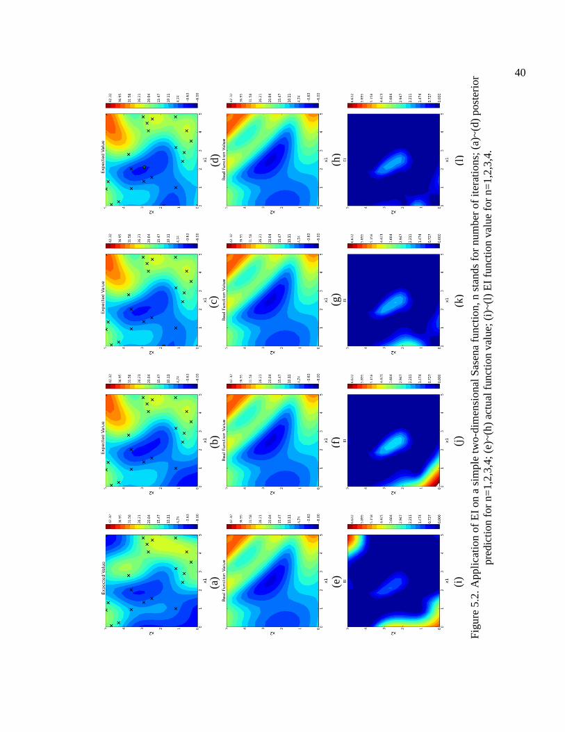
5.2. Application of EI on a simple two-dimensional Sasena function, n stands for number of iterations; (a)~(d) posterior prediction for n=1,2,3,4; (e)~(h) actual function value; (i)~(l) EI function value for n=1,2,3,4. ............................. 40

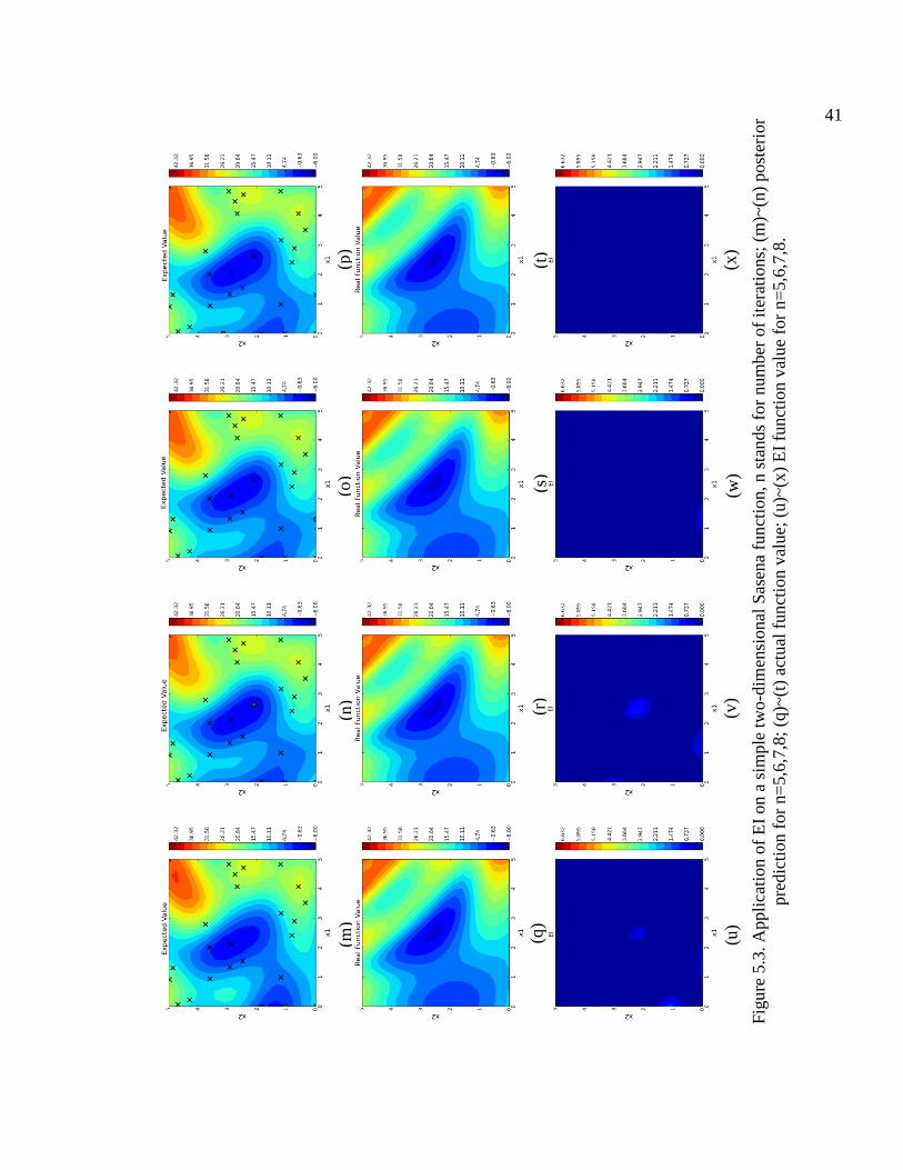
5.3. Application of EI on a simple two-dimensional Sasena function, n stands for number of iterations; (m)~(n) posterior prediction for n=5,6,7,8; (q)~(t) actual function value; (u)~(x) EI function value for n=5,6,7,8. ............................ 41

5.4. Application of EI on Harmant 3 function, sampling 50 times. ............................. 42 5.5. Application of EI on Harmant 6 function, sampling 50 times. ............................. 42 5.6. Application of extended EI on noisy 1D function, n stands for number of

iterations; (a)n=0;(b)n=2;(c)n=4;(d)n=5;(e)n=6;(f)n=41. ..................................... 43 5.7. Application of extended EI on noisy 1D function, with 3 initial observations.

............................................................................................................................... 44 5.8. Application of extended EI on noisy 2D Sasena function, with 20 initial

observations. ......................................................................................................... 44 6.1. Permeability field showing best well location by random search......................... 50 6.2. BGO with EI criterion for oil well placement prediction when oil price is

constant, starting with 5 observations and optimize 200 times. ........................... 50 6.3.

indicates frequentist well location and dot indicates predicted well location, respectively; (a) n=1;(b)n=50;(c)n=100;(d)n=125;(e)n=150;(f)n=195. ............... 51

6.4. Pareto Font line for NPV when oil price has uncertainty. .................................... 52 6.5. BGO with extended EI criterion for oil well placement prediction when oil

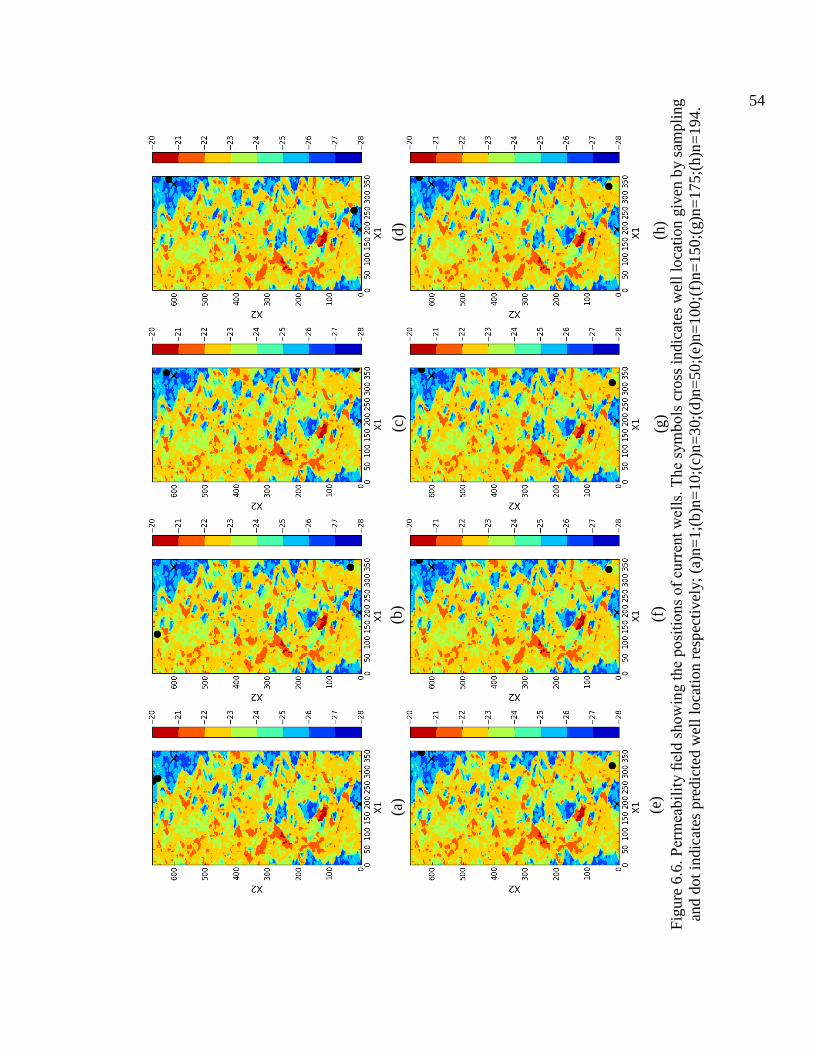
price has uncertainty. ............................................................................................ 53 6.6.

indicates well location given by sampling and dot indicates predicted well location respectively; (a)n=1;(b)n=10;(c)n=30;(d)n=50;(e)n=100;(f)n=150;(g)n=175;(h)n=194. .......... 54

6.7. BGO with extended EI criterion for oil well placement prediction when oil price and permeability has uncertainty. ................................................................ 55

vii

Figure ............................................................................................................................. Page

6.8. indicates well location given by sampling and dot indicates predicted well location; (a)n=1;(b)n=50;(c)n=200;(d)n=300;(e)n=400;(f)n=450;(g)n=475;(h)n=500. ...... 56

6.9. Histogram of net present value with 1000 samples. Green histogram line: oil price and permeability are both uncertain; Blue histogram: only oil price is uncertain. ........................................................................................................... 57

viii

LIST OF ABBREVIATIONS

NPV Net Present Value

BGO Bayesian Global Optimization

MC Monte Carlo

GPR Gaussian Process Regression

SE Squared Exponential

FVM Finite Volume Method

FDM Finite Difference Method

HGA Hybrid Genetic Algorithm

EI Expected Improvement

PDE Partial Differential Equation

GP Gaussian Process

MLE Maximum Likelihood Estimation

MAP Maximum a Posterior Probability

ix

ABSTRACT

Dou Zengyi. M.S.M.E., Purdue University, May 2015. Bayesian Global Optimization Approach to the Oil Well Placement Problem with Quantified Uncertainties. Major Professor: Ilias Bilionis, School of Mechanical Engineering.

The oil well placement problem is vital part of secondary oil production. Since the

calculation of the net present value (NPV) of an investment depends on the solution of

expensive partial differential equations that require tremendous computational resources,

traditional methods are doomed to fail. The problem becomes exceedingly more difficult

when we take into account the uncertainties in the oil price as well as in the ground

permeability. In this study, we formulate the oil well placement problem as a global

optimization problem that depends on the output of a finite volume solver for the two-

phase immiscible flow (water-oil). Then, we employ the machinery of Bayesian global

optimization (BGO) to solve it using a limited simulation budget. BGO uses Gaussian

process regression (GPR) to represent our state of knowledge about the objective as

captured by a finite number of simulations and adaptively selects novel simulations via

the expected improvement (EI) criterion. Finally, we develop an extension of the EI

criterion to the case of noisy objectives enabling us to solve the oil well placement

problem while taking into account uncertainties in the oil price and the ground

permeability. We demonstrate numerically the efficacy of the proposed methods and find

valuable computational savings.

1

CHAPTER 1. INTRODUCTION

1.1 Motivation

During secondary oil production water (potentially enhanced with chemicals) or gas

is injected to the reservoir through an injection well. The injected fluid pushes the oil out

of the production well. The oil well placement problem involves the specification of the

number and location of the injection and production wells, the operating pressures, the

production schedule, etc., that maximize the net present value (NPV) of the investment.

This problem is of extreme importance for the oil industry and an active area of research.

Several sources of uncertainty influence the NPV. The most important of these

sources are the time evolution of the oil price (aleatoric uncertainty) and our uncertainty

about the underground geophysical parameters (epistemic uncertainty). For convenience,

we will be referring to these uncertain parameters as stochastic inputs. Taking these

uncertainties into account, we see that the oil well placement problem constitutes a design

optimization problem under uncertainty. In this thesis, we consider the risk-neutral

approach of maximizing the expected NPV of the investment. Our developments are

easily extendable to the risk-averse case.

Given a set of design parameters as well as a realization of the stochastic inputs, the

computation of the NPV involves the solution of a coupled system of partial differential

equations (PDEs) describing the two-phase flow through the oil reservoir. In real scenario

2

involving complex large-scale reservoirs and/or multi-scale/physics modeling, simulation

times are exceedingly long making it impossible to solve the problem using standard

global optimization methods. Thus, there is an urgent need for global optimization

techniques that can work with a limited data acquisition budget.

There are various other difficulties associated with oil well placement problem. First,

note that the any optimization algorithm we employ needs to be gradient-free. Even

though the calculation of the gradient of the NPV with respect to the well locations is

theoretically possible using the method of adjoints, to the best of our knowledge, it has

not been done yet. Second, the high and potentially discontinuous variability of the

geophysical properties induces several local maxima in the NPV and necessitates a global

approach. Third, the computation of the expectation of NPV requires the computation of

high-dimensional integral (integration over all stochastic inputs). In a typical problem the

number of stochastic dimensions can well be in the order of hundreds of thousands. This

fact necessitates the use of a sampling or Monte Carlo (MC) approach. Fourth, the

characterization of the uncertainty of the geophysical properties requires the solution of

an inversion problem that fuses information from seismic surveys, data collected during

the primary production phase, analysis of ground specimens, and expert knowledge. Fifth,

the specification of the oil price model is a hard open problem in time series analysis.

The latter two difficulties constitute part of the formulation of the problem and are

not examined in detail. The novel contributions of this thesis focus on the solution of

stochastic optimization problems under uncertainty that face the following issues:

expensive data acquisition, lack of gradient information, and high-dimensional

3

uncertainties. We tackle these issues by employing and extending the method of Bayesian

global optimization (BGO).

BGO uses Gaussian process regression (GPR) to quantify our state of knowledge

about the objective function as captured by a finite number of evaluations. GPR is a

Bayesian meta-model. In contrast to classic meta-model approaches, it defines a

probability measure on the space of meta-models. This probability measure corresponds

to our uncertainty about the objective function as induced by the limited number of

observations we have at our disposal. BGO exploits this uncertainty to compute the

expected improvement (EI) of a new evaluation. In other words, it assesses the merit of

performing a new simulation by computing the EI it would bring to the current best

solution of the problem. By iteratively performing the simulations of maximum EI, BGO

gradually converges to the global optimum. The novel contribution of this thesis is the

extension of BGO to treat design optimization problems under uncertainty.

1.2 Literature Review

In the area of oil production, the fundamental research problems rise from the multi-

scale variability of the geophysical parameters such as the porosity and the permeability

of the ground.

Typically, the computational mesh is used to represent the reservoir in the sense that

the geophysical parameters are assumed to be constant within its computational cell.

Given the fact that this approach does not scale well as the reservoir becomes larger,

researchers focused on up-scaling maps to fill the gap between geological and simulation

grid size.[5, 20, 21, 41] Most recently, multi-scale techniques were proposed to solve the

4

large-scale problem using the fine scale geophysical information. This method is most

suitable for PDEs whose solutions display a multiple scale structure.[2, 3, 18, 28]. Since

the focus of this study is not on the modeling the oil reservoir, we will develop a simple

two-phase immiscible flow solver using the standard finite volume method (FVM). This

solver will constitute our oil reservoir simulator.

In the past, numerous of algorithms have been proposed for solution of optimization

and inverse problems in oil reservoir modeling.[36, 38] The selection of the optimal oil

well scheduling and placement problem using optimization algorithm was first studied

ten years ago.[6] Since then, wide arrays of methods have been proposed. For example,

Centilmen A et al. solves the problem by building a meta-model represented by artificial

neural networks[15, 25], Elamvazuthi et al. proposes a hybrid optimization technique

using fuzzy inference[23], Bittencourt develops a hybrid genetic algorithm (HGA)

optimization method that combines the polytope algorithm with neural network.[13]

Other researchers focus on more complicated aspects related to factors such as the well

type, the number of wells, and orientations or production characteristic parameters such

as porosity, permeability and so on. Although the research interest varies hugely, from

computational algorithm stand of point, they can be divided into two main catalogs: the

stochastic and the other is heuristic approach.[4] However, the existing literature has

barely touched the data acquisition problem as well as the high-dimensional aleatoric and

epistemic uncertainties.

In this study, we proposed a new approach for design optimization under uncertainty

with a limited data-budget and applied it to the well-placement problem in oil-reservoir

modeling. We developed an oil reservoir simulator based on the FVM that solves the

5

coupled PDEs describing the two-phase immiscible flow occurring during secondary oil

production. Based on limited observations, we construct a GPR to quantify our state of

knowledge about the NPV of the investment, and then use the EI data acquisition

criterion to actively select the most informative simulations. The remainder of this study

is organized as follows. Section 2 introduces a general background of physics and

mechanics of oil reservoir modeling, as well the numerical method we use to solve the

coupled PDEs. Section 3 proposes the target economical function, NPV, and discusses in

detail each quantity that affects it. Section 4 describes the GPR for construction of meta-

models. Section 5 discusses data-acquisition criteria for design optimization. Section 6

shows the results for several different testing scenarios and conclusions are given.

6

CHAPTER 2. PHYSICS AND MATHEMATICS MODEL FOR OIL RESERVOIR

In this section, we introduce all critical physical parameters to mathematical model

describing an oil reservoir during secondary oil production. The physics involve a two-

phase immiscible flow which can be described via a coupled PDE system. We conclude

by discussing the details of the numerical solution of the coupled PDEs.

2.1 Porosity

In geoscience, the holes in sandstones are called porosity. Porosity is a measure of

space not occupied by the solid rock, also defined as volume fraction of total rock

occupied by other phase such as water, oil or gas.[1] Usually rock porosity is denoted by

, and it is a number between 0 and 1. Strictly speaking, oil and gas are not stored as a

continuous empty space. Instead, they are in the space between grains and sandstones.

Rock is treated as a compressible material like a sponge although in reality it is hard and

appears solid. Mathematically, the compressibility of rock is defined as:

1

,r

dc

dp (2.1)

where p refers to overall pressure in the reservoir. In order to simplify the model, in this

study we assume there is no compressibility, which means porosity only depends on

spatial coordinate.

7

2.2 Permeability

Permeability is a tensor quantity that measures the ease with which a fluid (in this

study, either water or oil) can move through a porous rock. Permeability is denoted as K ,

and typically has unit of darcy (D) or millidarcy (mD). In petroleum production,

millidarcy is used more often, for 1 darcy is a relatively huge number. A more accurate

definition is that 1 darcy is equal to 1 cp fluid flow through a homogeneous material at

1cm/s speed under 1 atm/cm pressure gradient.[1]

phase or fluid. If there is more than one phase, the effective permeability of a specific

phase depends also on the other phases existing at the same location. This is, of course, a

coarse model since the two phases do not mix with each other from a microscropic

perspective. This effective permeability, a nonlinear function of absolute permeability K

and saturation s , will be called relative permeability. Relative permeability is the ratio of

effective permeability of a particular fluid at a particular saturation to the absolute

permeability of that fluid at total saturation:

1( ),i ri ik sK K (2.2)

where i stands for the phase or liquid we are interested and 1i stand for the other

phase. Generally speaking, relative permeability is determined by pore-size, the viscosity

of the two phases, and the forces between the fluids.[22] These factors are easily taken

into account. The challenging part in secondary oil production is the significant, non-

trivial temperature dependence of the permeability.[34]

The measurement of permeability is costly and difficult.[27] Even using the latest

techniques and instruments, there is still a lot of residual uncertainty that makes the result

8

of the numerical simulator untrustworthy. Thus, when making the well developing plan,

it is better to consider the uncertainty of the permeability field.

Permeability data can be collected in three ways. First, permeability information can

be extracted from seismic surveys.[40] Second, permeability can be derived from through

Bayesian model inversion using data collected in primary production stage.[10, 12] Third,

small scale permeability measurements can also be gathered through drilling and then

used to construct an upscaled version of the permeability field.[44] No matter which

method is used to get permeability data, there will always be some residual uncertainty.

Since permeability uncertainty directly affects production rate, it should not be ignored.

In this study, we construct a synthetic, albeit realistic, stochastic permeability model

based on the data included in the SPE Comparative Solution Project.[21] Namely, we

model the logarithm of the permeability as a Gaussian process.[24] Specifically:

0ln ( ) ln ( ) ( ),

wher Ge g( ) ( ( ) | 0, ( , ) ,P )s s s

s

K K g

g k

x x x

x (2.3)

where K(xs ) is the permeability at the spatial location xs = (xs1,xs2

) , and g(xs ) is a

Gaussian distribution with an exponential covariance function:

'

2

1

( ) exp .s

di i

i si

x xk v

lx,x' (2.4)

To make matters worse, permeability may change during the production process, as

well as when the environment temperature and pressure change. Permeability also

depends on the direction and fluid type, i.e. permeability is not isotropic and constant

property for different fluids. So it could have different values when different fluids

9

passing through the same rock sample. In this study, however, we assume the rock is an

isotropic material and permeability is a constant real number.

2.3 Fluid Properties

In secondary oil production, the empty space in the rock is filled with either aqueous

phase or oleic phase. The concept of saturation is introduced to describe the volume

fraction occupied by different phases. For multiple phases, following relationship always

holds:

1,iallphases

s (2.5)

In this study, we consider a two-phase flow. One phase is the aqueous phase which

mainly contains water and the other one is oleic phase mainly contains hydrocarbon. In

two phase flow model, there is no need to distinguish whether the oleic phase consists of

gas or oil. The conservation of mass gives rise to the following relationship:

1 1

1,N N

io iwi i

c c (2.6)

where the mass fraction of i in phase j is written as ijc . For the viscosity i and density

i , we have:

1( , ,... ),i i i i Nip c c (2.7)

1( , ,... ).i i i i Nip c c (2.8)

Due to interfacial tension, different phases have different phase pressure ip . The

capillary pressure is defined to be:

,cij i jp p p (2.9)

10

where , ,i j o w . Although the capillary pressure depends on many properties, we

assume that it is the function of saturation only.

2.4 Mathematical Model of an Oil Reservoir

Fluid motion can be described by the conservation of mass, momentum, and energy

and thermodynamics. Oil production is not an exception. The momentum equation is

incl

between fluid velocity and the pressure gradient.

In this study, we use the immiscible two-phase oil model, based on the assumption

that the capillary effect is neglected. For more precise model considering the capillary

effect more information can be found in [19]. As mentioned before, we consider an

aqueous and oleic phase, assuming only water is in the aqueous phase and that the oleic

phase contains hydrocarbon mixture. The following PDEs are used to describe the two-

phase flow throug

pushes water and oil through porous rock is gravity and the pressure gradient. Each phase

has each own continuity equation:

( )

( ) ,i ii i i

sv q

t (2.10)

where i stands for either aqueous phase or the oleic phase. Expanding the Equation

(2.10), we obtain a more detailed form of continuity equation:

.i i i i i ii i

i i i

s s v qs v

t t t (2.11)

Before plugging the pressure equation into the continuity equation, let us introduce

the concept of phase mobility defined as /i ri ik . According to Equation (2.5),

11

saturation of oil and water has the relationship: 1w os s , then sum continuity equation

of aqueous phase or oleic phase and define / /w w o oq q q , we have:

( ) .w w o o w w o ow o

w o w o

s s v vv v q

t t t (2.12)

The oil wells either produce oil and water mixture or inject water. The source term q

on the right hand side in the Equation (2.12) is non-positive at the location of a

production well and non-negative at the location of an injection well. In real production

process, both injection and production wells are subject to control and optimization.

Darcy discovered an empirical equation that connects the volumetric flow density v

to the pressure :

( ).rii i i

i

kv p g zK (2.13)

As mentioned before, since the purpose of this study is not to set up an extremely

precise oil simulator, assumption that rock and two fluid phases are incompressible is

reasonably proposed to simplify the problem. quation

(2.12), it reduced to:

,

[ ( ) ( )].w w w o o o

v q

v p g z p g zK K (2.14)

In Equation (2.14), there are two unknown phase pressure op and wp . The normal

solution is introducing the capillary pressure cow o wp p p , which is regarded as a

function of water saturation ws . However, this makes the saturation and pressure

equations strongly coupled. So another approach, using global pressure p is introduced.

Also, we assume that the capillary pressure cowp is a monotone function of the water

12

saturation ws .Global pressure is defined as: o cp p p , where the complementary

pressure cp is defined by:

1

( ) ( ) ( )d ,ws

cowc w w

w

pp s f

s (2.15)

where / ( )w w w of is factional-flow function that measures the water fraction of the

total flow. Finally, introducing the total mobility w o , we obtain the following

elliptic equation for the global pressure p :

[K p K( w w + o o)gz] = q. (2.16)

The pressure equation gives us the first primary unknown p . The secondary

unknown ws is introduced in the saturation equation:

( )[ ( , ) ( )] .w ww w w w w

w

s qf s v d s s g s

t (2.17)

2.5 Numerical Implementation: Finite Volume Method

The most basic method for the solution of PDEs is the finite difference method

(FDM). This method is based on a finite difference approximation of the partial

derivatives of the solution occurring in the PDEs. In this study, we use the finite volume

method (FVM). FVM is derived from the conservation of physical quantities over cell

volumes and is, therefore, consistent with them. In FVM, the unknown functions or

-volumes, over

which the integrated PDE model is required to hold in an averaged sense. The hidden

assumption is that the flux that leaves one small volume is equal to the flux that enters

another adjacent volume, so that continuity equation is valid automatically.

13

2.6 Solution Strategies for Coupled System

Based on the derivation in previous section, the fractional-flow model for immiscible

two-phase flow can be described using pressure Equation (2.16) and saturation Equation

(2.17). These two equations are nonlinearly coupled through the saturation-dependent

mobilities i . In addition, they are also coupled through other parameters that depend on

pressure or saturation. The classic way to solving coupled PDEs is to make an implicit

discretization for each equation and then solve for the two unknowns together. However,

due to numbers of iterations required, this way is too expensive especially for large

nonlinear systems of equations. In this study, we apply another method called sequential

splitting method. This method is designed as follows: First, before the global pressure and

total velocity are solved for, the data from the previous time step is used to compute the

saturation-dependent coefficient in Equation (2.16). Then, total velocity v is kept as a

constant parameter in Equation (2.17), while saturation is advanced. Next, saturation-

dependent coefficients in Equation (2.16) are updated, and the pressure equation is solved

again and so on. Finally, the numerical scheme is developed without considering the

coupling problem between the two equations.

Although this splitting method will introduce an error by decoupling the equations,

its efficiency makes up for it.

14

CHAPTER 3. OBJECTIVE FUNCTION-NET PRESENT VALUE

3.1 Net Present Value

There are three major factors that we need to consider when computing the NPV of

an oil reservoir investment. Those are: the profits we make by selling the oil we extract,

the operation costs of running the production plan, and the water disposal costs.

The most important factor that affects the NPV is amount of crude oil that comes out

of the production well as a function of time. Due to the complicated economic

environment, crude oil price fluctuates constantly and, thus, needs to be modeled as a

stochastic process. To further complicate matters, the producer may decide to sell the oil

right away or store it in anticipation of better prices. In this study, we will assume that the

producer sells the oil at the current market price. In our numerical examples, we will

investigate two different cases of price models: a time independent constant price model

and a log-normal random walk price model.

The second NPV factor is the operation cost. This includes the cost of pumping

water into the injection well, as well as the cost of the equipment and labor. Since the

cost of equipment and labor remains constant, if we do not optimize over the number of

wells, we ignore it in our analysis. Furthermore, we assume that the cost of water

injection is proportional to the rate of injection and constant over time.

15

The third and final cost we consider is the cost associated with the disposal of waste.

Water coming out of the production well is highly contaminated and has to be disposed

according to the local environmental protection laws. Here, we also assume that the cost

of water disposal is proportional to the rate with which waste water is produced and does

not vary with time.

Putting all this considerations together and using a discount factor r , we can write

the NPV of the investment over a time period T as:

,0

.

/365

,.

( ) { [( ( ) ( , ) ( , ))]

( , )} / (1 )

T

T o o w disp wprod wells

t

w inj winj wells

f c t q t c q t

c q t r dt

x x x

x (3.1)

The implicit assumption here is that all the other operation expenses (lifting,

separation, filtering, pumping and reinjection and so on), are independent of well location

and can, thus, be excluded from our analysis. In Equation (3.1), c stands for unit cost of

the quantity . In our numerical simulations, we take the cost for water injection to be

0.03$/bbl and the cost for water lifting is 0.04$/bbl. As mentioned already, we explore

two cases of oil price: constant and log-normal random walk. The latter is discussed in

Sec. 3.2. In Equation (3.1) q stands for flow rate of the quantity and it is a function

of the well locations as well as of time. The flow rate functions are implicitly defined

through the solution of the two-phase flow PDEs which we introduced in Chapter2.

The design problem we wish to solve is:

x* = argmaxx fT (x), (3.2)

subject to the constraint that the well locations x must lie within the reservoir.

17

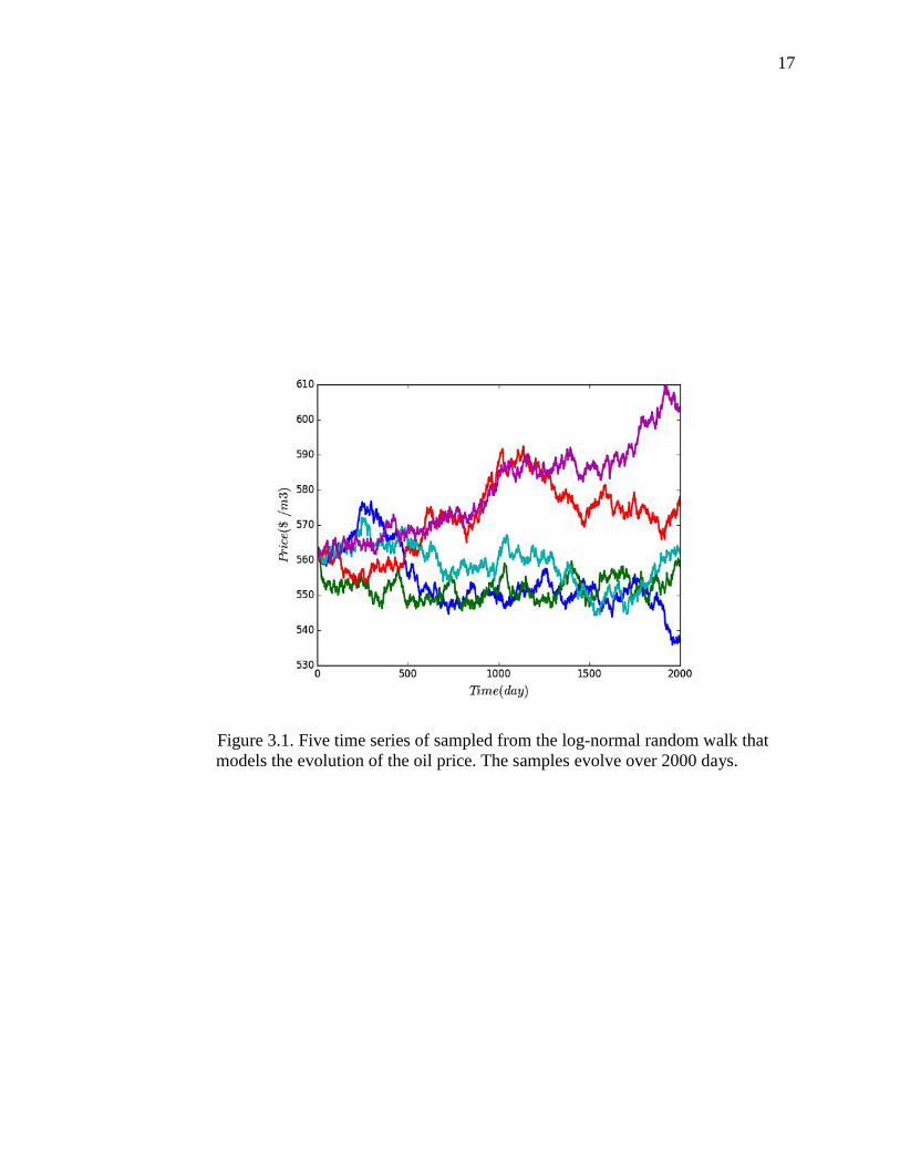
Figure 3.1. Five time series of sampled from the log-normal random walk that models the evolution of the oil price. The samples evolve over 2000 days.

18

CHAPTER 4. GAUSSIAN PROCESS REGRESSION

The optimization of the oil well placement problem using directly the oil reservoir

simulator is computationally infeasible. Therefore, it is essential to replace the (expected)

NPV function with a cheap-to-evaluate meta-model (surrogate). The meta-model we use

in this work is Gaussian process regression (GPR). [28]

GPR is the Bayesian interpretation of classical Kriging regression techniques.[42] It

is a powerful non-linear and non-parametric regression technique that has the added

benefit of being able to quantify the epistemic uncertainty induced by the limited

observations. As we show in Chapter 5, this uncertainty is the key for deriving

information acquisition policies. Here, we cover the mathematical background of GPR

covering its formulation as well as the model selection techniques required for selecting

the hyper-parameters that describe the covariance function.

4.1 Using Gaussian Processes to Represent Prior Knowledge

A Gaussian process (GP) is a generalization of multivariate normal distribution

(MVN) to infinite dimensions. For completeness, let us state here the probability density

of a MVN in D dimensions:

11/2/2

1 1( | , ) exp[ ( ) ( )],

2(2 )T

DN x (4.1)

19

where is the mean vector, and is the covariance matrix. Notice that the dimension of

is 1D while the covariance matrix is a D D symmetric positive-definite matrix.

A GP is an extension of this MVN to the space of function. In other words, a GP defines

a probability measure on a function space. We interpret this probability measure as our

prior knowledge about the function before we see any data. In analogy to a MVN, a GP is

defined via its mean and covariance, albeit those are now functions. We write:

f (×) | m(×),k(×,×) ~ GP( f (×) | m(×),k(×,×)), (4.2)

where ( ) : Dm n n is the mean function and , ) :( D Dk n n n is the covariance

function. Therefore, compared to a multivariate normal we have:

A random function ( )f instead of a random vector x .

A mean function ( )m instead of a mean vector .

A covariance function ( , )k instead of a covariance matrix .

Note that the mean function is arbitrary while the covariance function has to be a positive

definite function.

In our core example, x is four dimensional (D=4) and corresponds to the location of

the injection and the production wells, and ( )f represents the (expected NPV).

The meaning of Equation (4.2) comes through the MVN. In particular, consider an

arbitrary set of N input points represented as an N D matrix:

(4.3)

as well as the set of function responses on these points represented as an N dimensional

vector:

21

4.2 Covariance Function

In supervised learning, the concept of the covariance function models similarity

between observations. The underlying expectation is that when two observations have

similar inputs, then they are likely to have similar outputs. In this way, observations that

are close to a query point can provide useful information for prediction. Thus the

covariance function is an indispensable part of GPR. It encodes the assumptions about the

function we wish to learn.

Another name for a covariance function k(×,×) is kernel. In general, the choice of the

covariance function depends on the prior assumptions about the regularity of the function

space. However, it is usually true that kernels are non-negative k(x,x ) 0 and that as

the distance between x and x increases k(x,x ) becomes smaller. Some commonly

used covariance functions are the squared exponential (SE), the exponential covariance,

the linear covariance, the polynomial covariance, the rational quadratic covariance, and

the periodic covariance. All of these covariances have free parameters , which are

known as hyperparameters.

In this study, we assume that our prior belief of objective function ( )f x conforms

with a GP zero prior mean and a squared exponential (SE) covariance:

k(x,x ') = s2 exp

1

2

(xi xi ')2

li2

i=1

D

+ 2 x x '( ), (4.10)

where the hyperparameters must satisfy 0s and li > 0 . Here li is the characteristic

length-scale of the i-th input. Intuitively, it measures how far we need to move in order to

make function value of two input points uncorrelated. The SE covariance function

22

implements automatic relevance determination (ARD). [33] That is, if li has a large value

then covariance will becomes independent of input i. The parameter s is interpreted as

the signal strength. In words, the bigger it is, the more do sample function ( )f from the

corresponding GP vary about the mean. The last part of the right hand side models

delta. It is assumed

to be zero unless the two inputs correspond to the same measurement. When we know

that our observations are noiseless, then we just set the noise level equal to zero. We

only use it when we want to represent the uncertainty in the NVP.

To conclude this section, let us mention once more that the GP constructs a prior

probability measure on the space of meta-models which quantifies our state of knowledge

about the function of interest. To emphasize this, we will also denote Equation. (4.5) by:

f (×) ~ p( f (×)). (4.11)

In the following section, we show how observations can be combined with this prior

measure using Bayes theorem, to get the posterior probability measure:

(4.12)

The latter is a representation of our state of knowledge about the objective function that is

compatible with both the prior knowledge as well as the observations.

4.3 Conditioning a Gaussian Process on Observations

Assume that we have observed a set of N inputs and outputs as

defined earlier. Conditioning the prior on this data using the Bayes rule, we get the

posterior GP measure:

23

(4.13)

where ( )nm x as the posterior mean function:

mN (x) = m(x) + k N (x)K N1(mN fN ), (4.14)

and ( , ')nk x x is the posterior covariance function:

kN (x,x ') = k(x,x ') kN (x)T K N1kN (x '). (4.15)

Even though Equation (4.13) contains all posterior information, it is usually more

convenient to work with the point predictive distribution:

(4.16)

where the posterior predictive variance is simply given by:

N2 (x) = kN (x,x). (4.17)

4.4 Hyper-parameter Selection

In GPR we estimate the hyper-parameters of the covariance function using Bayesian

model selection tools. In this study, we use the SE covariance function as default and

model selection will be used to find the optimal values for each parameters: the signal

strength, the length scale of each dimension, and (if required) the noise level.

The fully Bayesian approach for model selection would be to assign a prior on the

hyper-parameters and then characterize their posterior using sampling techniques.

However, if the observations are not enough and prior information about the hyper-

parameters is vague (e.g., if we assume uniform priors), then one usually obtains good

results simply by maximizing the likelihood of the data (y | X, )p . Since likelihood

function is positive, we choose to work with its logarithm. The log likelihood of GPR can

be written as:

24

log p(fN | XN , ) = 1

2fN

TK N1fN

1

2log K N

N2

log2 , (4.18)

where K N is the covariance matrix and ={s,1, , D , 2} represents all the hyper-

parameters of the model. It can be shown that the gradient of the log-likelihood is:

j

log p(fN | XN , ) = 1

2fN

TK N1 K N

j

K N1fN

1

2tr(K N

1 K N

j

)

= 12

tr((a NaNT K N

1)K N

j

),

(4.19)

where aN = K N1fN .

We solve the log-likelihood maximization problem using the BFGS algorithm[14].

To deal with the positive constraints on the hyper-parameters we work with their

logarithms.

25

CHAPTER 5. BAYESIAN GLOBAL OPTIMIZATION

In this section we address the problem of solving the following design optimization

problem:

* argma ( ,x )fx xx (5.1)

under a limited evaluation budget for the objective function. To start with, assume that

we have observed some, initially randomly picked, evaluations of the objective function

and that we have built, using the methodology of Chapter 4, a GP representing our

posterior state of knowledge. We may use this state of knowledge about the objective to

quantify our state of knowledge about the solution to the design optimization problem.

A naïve, but very common approach to characterize our state of knowledge about the

optimal solution, would be to replace the objective function with the posterior mean

function of the GP characterizing our posterior state of knowledge. Since the posterior

mean function is very cheap to evaluate, we may then proceed to solve the design

optimization problem. Even though this approach is appealing it hides a lot of problems

the most important of which is that the accuracy of the solution we find depends on the

accuracy of the surrogate surface.

26

The idea in Bayesian global optimization (BGO) is to interrogate the posterior GP

for design points of high expected value and sequentially iterate between making the

most valuable observations and conditioning the posterior GP on them until our data

acquisition budget is exhausted. Stating the problem in its full mathematical generality

results in a very hard dynamic programing problem.[39]

Since the data acquisition problem in its most general form is computationally

intractable, we restrict our attention to the more modest goal of finding good sequential

one-step-look-ahead data acquisition policies. These data acquisition policies are also

called myopic data acquisition policies. A good myopic data acquisition policy must

include a tradeoff between two competing goals: exploration and exploitation.

Exploration refers to our need to have strategies that broadly explore the design space on

which we are largely uncertain about the value of the objective. Exploitation refers to the

desire to use our existing knowledge that the objective is high on certain regions of the

design space, zoom in those regions and search for an even better solution. As we will see

later on, in BGO, exploration is related to the posterior variance and exploitation to the

posterior mean of the GP representing our state of knowledge about the objective.

In what follows, we discuss generic myopic data acquisition policies (Sec. 5.1)

including special choices suitable for design optimization involving deterministic

surrogates (Probability of improvement in Sec. 5.1.1 and expected improvement in Sec.

5.1.2) and provide special examples 5.1.3. In Sec. 5.2, we propose a generalization of the

expected improvement data acquisition policy to the case of design optimization under

uncertainty and demonstrate the efficacy of our approach using numerical examples.

27

5.1 Acquisition Functions for Bayesian Optimization

Assume that we have made N observations and that our posterior state of

knowledge can be neatly summarized through the point predictive distribution given in

Equation (4.16):

Our problem in this section is to find the most valuable design point 1Nx to observe

next. The core idea behind the proposed solution is founded on the concept of the value

of information.[32] Specifically, assume that we made a hypothetical new observation at

point x and that the objective function value was y . Denote by v(x, y;Dn ) the value of

making this observation. Since, we do not actually know what y could be, we have to

integrate it out of the picture using the point predictive distribution of the posterior GP as

Equation. (4.16). Doing this, we may define the expected value of observing x :

(5.2)

We are now in a position to define a myopic data acquisition policy associated with

value function. It boils down to a sequential iterative solution of optimization problem:

(5.3)

That is, the myopic optimization policy sequentially observes the objective function

on the design points expected to be most valuable. A natural stopping criterion for such a

generic policy is to stop when the maximum expected value of the current iteration of the

policy is smaller that a threshold. Mathematically, we may stop when:

(5.4)

where is a an arbitrary tolerance.

28

In real applications, one must pay special attention to avoid stopping prematurely

due to the S-curve phenomenon of information.[39] The S-curve phenomenon expresses

the possibility that in many problems exhibit three distinct faces when it comes to

information collection. Initially, when data is limited, a single observation might not be

informative enough for the objective a fact that is demonstrated with a small value.

However, as more data is accumulated, individual observations start becoming more

valuable. This behavior can be attributed to the fact that the GP has learnt exploitable

information from the data. Finally, as we keep getting closer to the objective, individual

-

avoid the very first concave part of t

do not stop before a specific number of observations have been made.

In the rest of this subsection, we discuss two choices for the value function: The

probability of improvement (PI) and the expected improvement (EI).

5.1.1 Probability of Improvement

The probability of improvement (PI) policy sequentially picks the design that is most

likely to yield an improvement over the current maximum.[31] In particular, let

(5.5)

be the current observed maximum value. PI picks the design point x that has the highest

probability (according to posterior GP) a value greater than :

(5.6)

30

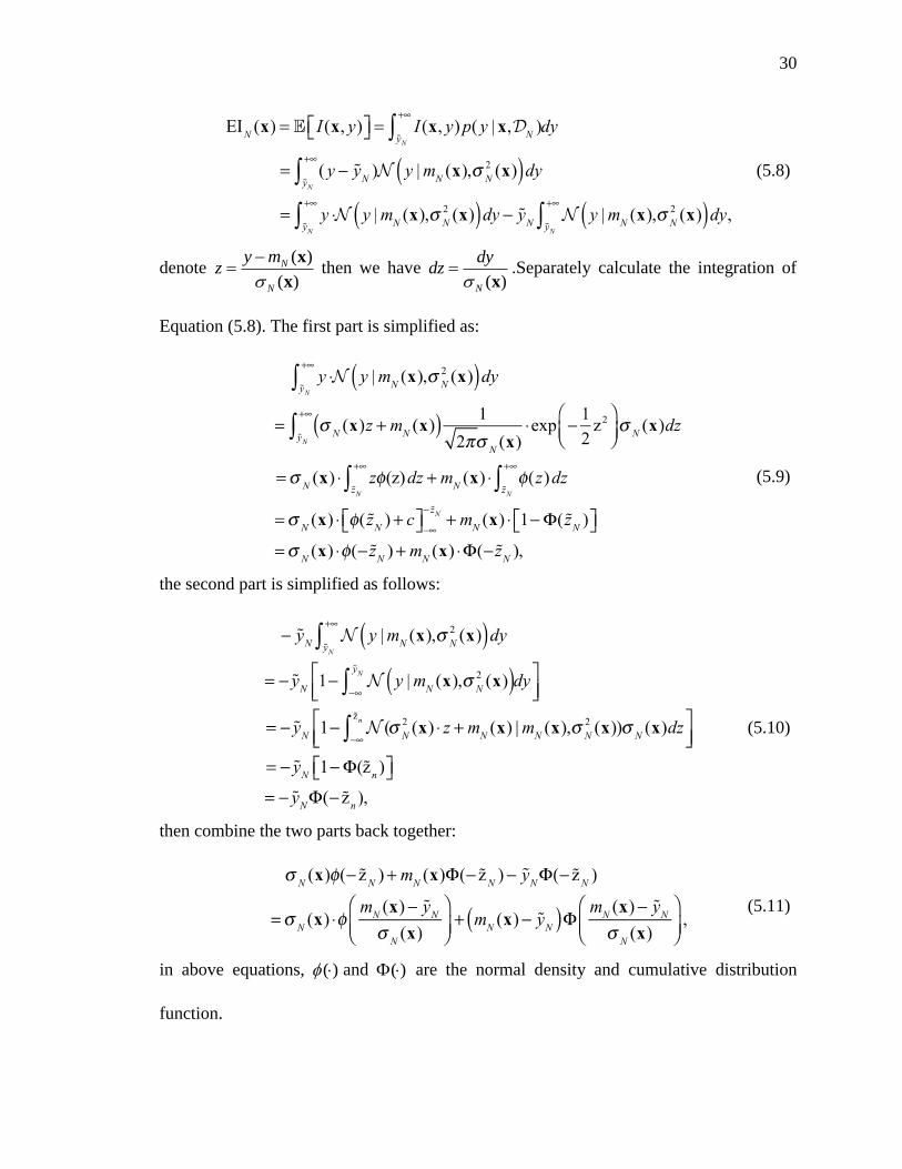
(5.8)

denote (

( )

)N

N

y mz

xx

then we have ( )N

dydz

x.Separately calculate the integration of

Equation (5.8). The first part is simplified as:

(5.9)

the second part is simplified as follows:

(5.10)

then combine the two parts back together:

(5.11)

in above equations, ( ) and ( ) are the normal density and cumulative distribution

function.

31

Then, the point s the expected

improvement, i.e.:

x* = argmaxEIN (x). (5.12)

Summarizing, the expected improvement after observing an arbitrary point is

(5.13)

If our objective was to find the global minimum (instead of the global maximum), then

we would have:

(5.14)

where now is the current observed minimum (instead of the current observed

maximum).

5.1.3 Applications

In this section, we explore the performance of the EI policy on some toy objective

functions. We start with a simple one dimensional example. Our aim is to find the global

maximum of:

2 2( ) 4 sin 20 ( 0.5) cos(20 0.1) ,

[0,1].

f x x x

x (5.15)

We start with a randomly selected set of 6 function evaluations. Then we apply the

Gaussian process methodology of Chapter 4 in order to construct the posterior measure

representing our state of knowledge based on this initial pool of data. The mean of this

posterior Gaussian process is the blue line of Figure 5.1(a) while the 95% credible

interval is shown by the grey shaded area. This blue line is to be compared to the red line

32

which depicts the true, albeit unknown, objective function. In the same plot, we show the

expected improvement as a function of the design space (green dashed line). The most

informative observation (to be made next) is marked with a green disk. Figures 5.1(b-f)

We can see that as the

number of iterations increases, the posterior mean gets closer to the actual objective

function, especially, in the area around the actual global maximum. The value of the

expected improvement, shown on the right-hand scale, is gradually decreasing. This fact

indicates the observations become less and less informative.

The second example we consider is 2D objecti Sasena

asena function is defined by:

2 2 2 2

2 1 1 2 2 1 2

1 2

( ) 2 0.01 ( ) (1 ) 2 (2 ) 7sin(0.5 ) sin(0.7 ),

0 5,0 5.

y x x x x x x x

x x

x (5.16)

In this test, the aim is to find global minimum. The starting observation pool consists

of twenty randomly picked design points. We present the results in Figure 5.2 and Figure

5.3. This numerical example demonstrates that the EI policy balances exploration and

exploitation. At first two iterations the new points chosen are not close to the currents

minimum region. The reason they are chosen is due to their high predictive uncertainty.

During this phase, EI actually explores. After this phase, the last six observations are all

around the current minimum region. This corresponds to the exploitation phase. Finally,

notice the dramatic decrease of the EI as the number of iterations increases. This behavior

is identical to the one we observed in the 1D toy example.

33

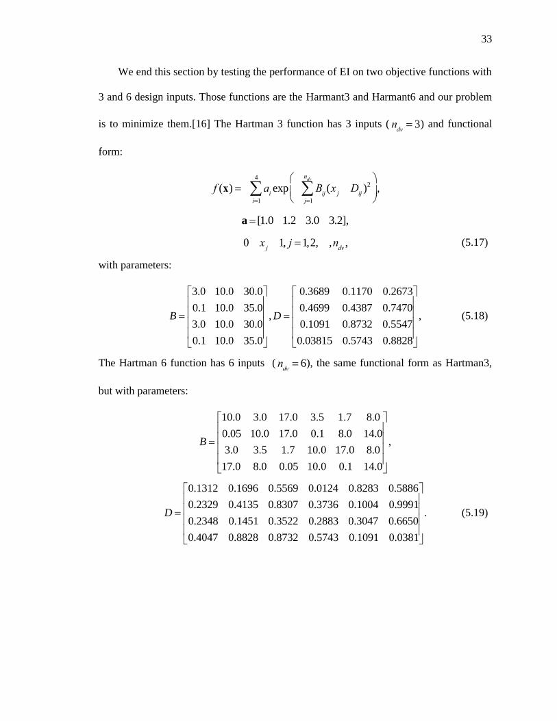
We end this section by testing the performance of EI on two objective functions with

3 and 6 design inputs. Those functions are the Harmant3 and Harmant6 and our problem

is to minimize them.[16] The Hartman 3 function has 3 inputs ( ndv = 3) and functional

form:

f (x) = ai exp Bij (x j Dij

j=1

ndv

)2

i=1

4

,

[1.0 1.2 3.0 3.2],a

0 x j 1, j = 1,2,� ,ndv , (5.17)

with parameters:

3.0 10.0 30.0 0.3689 0.1170 0.2673

0.1 10.0 35.0 0.4699 0.4387 0.7470, ,

3.0 10.0 30.0 0.1091 0.8732 0.5547

0.1 10.0 35.0 0.03815 0.5743 0.8828

B D (5.18)

The Hartman 6 function has 6 inputs ( ndv = 6), the same functional form as Hartman3,

but with parameters:

10.0 3.0 17.0 3.5 1.7 8.0

0.05 10.0 17.0 0.1 8.0 14.0,

3.0 3.5 1.7 10.0 17.0 8.0

17.0 8.0 0.05 10.0 0.1 14.0

B

0.1312 0.1696 0.5569 0.0124 0.8283 0.5886

0.2329 0.4135 0.8307 0.3736 0.1004 0.9991.

0.2348 0.1451 0.3522 0.2883 0.3047 0.6650

0.4047 0.8828 0.8732 0.5743 0.1091 0.0381

D (5.19)

34

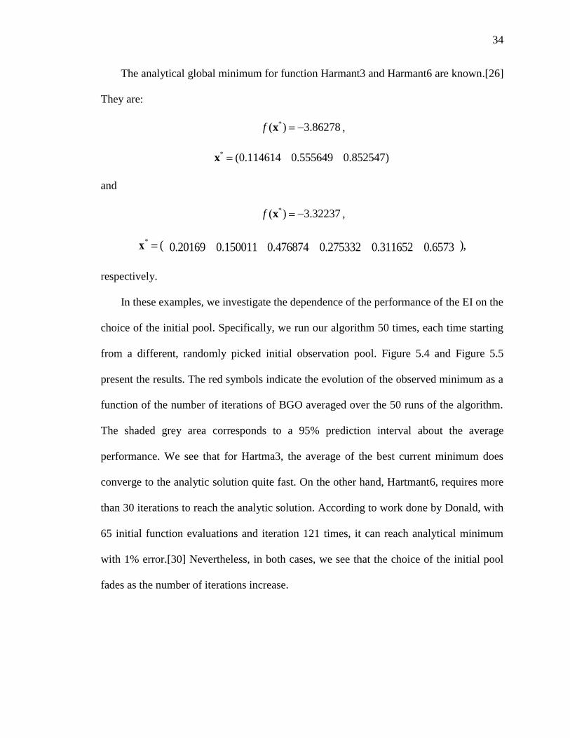
The analytical global minimum for function Harmant3 and Harmant6 are known.[26]

They are:

*( ) 3.86278f x ,

* (0.114614 0.555649 0.852547)x

and

*( ) 3.32237f x ,

x* = ( 0.20169 0.150011 0.476874 0.275332 0.311652 0.6573 ),

respectively.

In these examples, we investigate the dependence of the performance of the EI on the

choice of the initial pool. Specifically, we run our algorithm 50 times, each time starting

from a different, randomly picked initial observation pool. Figure 5.4 and Figure 5.5

present the results. The red symbols indicate the evolution of the observed minimum as a

function of the number of iterations of BGO averaged over the 50 runs of the algorithm.

The shaded grey area corresponds to a 95% prediction interval about the average

performance. We see that for Hartma3, the average of the best current minimum does

converge to the analytic solution quite fast. On the other hand, Hartmant6, requires more

than 30 iterations to reach the analytic solution. According to work done by Donald, with

65 initial function evaluations and iteration 121 times, it can reach analytical minimum

with 1% error.[30] Nevertheless, in both cases, we see that the choice of the initial pool

fades as the number of iterations increase.

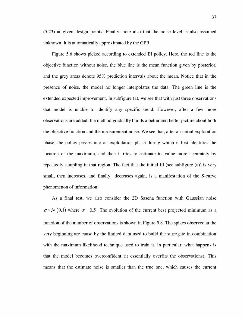
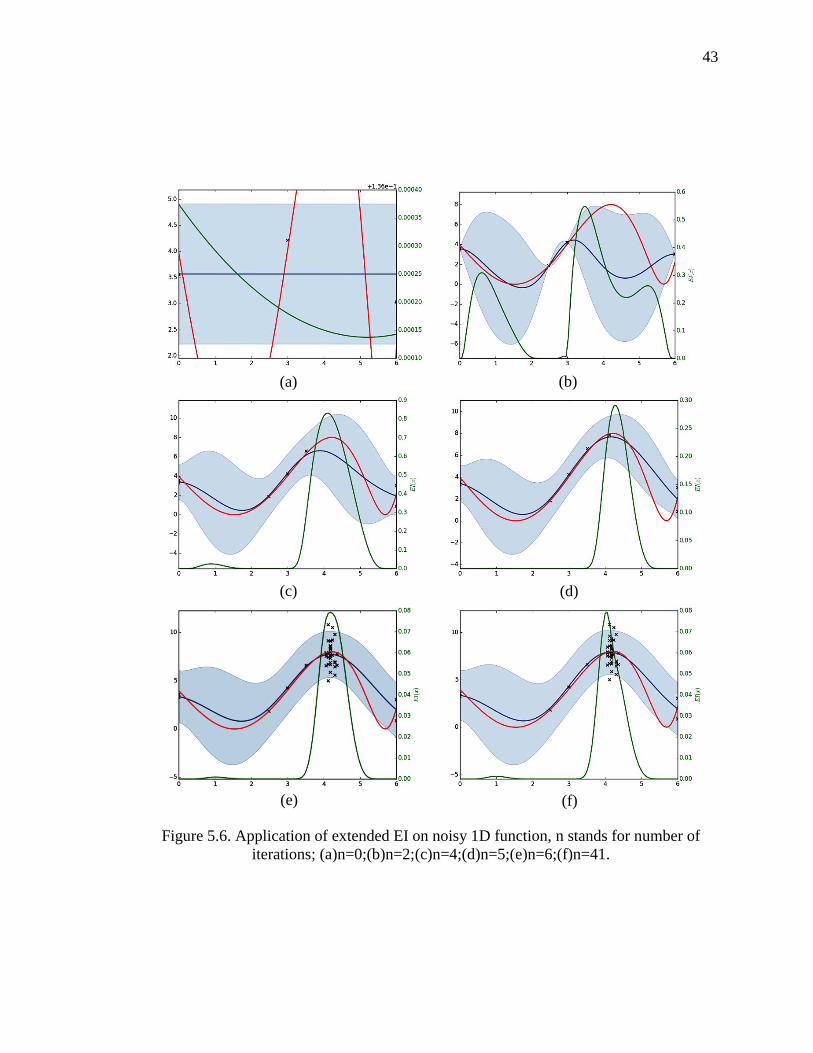
38

projected minima to be closer to the noise-contaminated current observed minima. The

situation is gradually remedied as more observations are made.

Based on all results above, we can conclude that the extended EI policy maintains all

the advantage that EI. At the same time, it can successfully approach to global optimum

even with noisy objective function observations.

39

Figure 5.1. Application of EI on a simple one-dimensional test function. Start with 6 initial observations; n stands for number of iteration

(a)n=1;(b)n=2(c)n=3;(d)n=4;(e)n=5;(f)n=6.

(e) (f)

(c) (d)

(a) (b)

40

Figu

re 5

.2. A

pplic

atio

n of

EI

on a

sim

ple

two-

dim

ensi

onal

Sas

ena

func

tion,

n s

tand

s fo

r nu

mbe

r of

iter

atio

ns; (

a)~(

d) p

oste

rior

pr

edic

tion

for

n=1,

2,3,

4; (

e)~(

h) a

ctua

l fun

ctio

n va

lue;

(i)

~(l)

EI

func

tion

valu

e fo

r n=

1,2,

3,4.

(a)

(b)

(c)

(d)

(e)

(f)

(g)

(h)

(i)

(j)

(k)

(l)

40

41

Figu

re 5

.3. A

pplic

atio

n of

EI

on a

sim

ple

two-

dim

ensi

onal

Sas

ena

func

tion,

n s

tand

s fo

r nu

mbe

r of

iter

atio

ns; (

m)~

(n)

post

erio

r pr

edic

tion

for

n=5,

6,7,

8; (

q)~(

t) a

ctua

l fun

ctio

n va

lue;

(u)

~(x)

EI

func

tion

valu

e fo

r n=

5,6,

7,8.

(m)

(n)

(o)

(p)

(q)

(r)

(s)

(t)

(u)

(v)

(w)

(x)

41

42

Figure 5.4. Application of EI on Harmant 3 function, sampling 50 times.

Figure 5.5. Application of EI on Harmant 6 function, sampling 50 times.

43

Figure 5.6. Application of extended EI on noisy 1D function, n stands for number of iterations; (a)n=0;(b)n=2;(c)n=4;(d)n=5;(e)n=6;(f)n=41.

(a) (b)

(c) (d)

(e) (f)

44

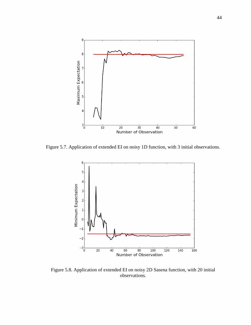
Figure 5.7. Application of extended EI on noisy 1D function, with 3 initial observations.

Figure 5.8. Application of extended EI on noisy 2D Sasena function, with 20 initial observations.

45

CHAPTER 6. AN APPLICATION: WELL PLACEMENT PROBLEM

In the oil well placement problem, our aim is to identify the best well location that

can maximize NPV function. Due to limited budget, computational difficulties, and the

uncertainty in the specification of the oil price as well as the permeability, this problem is

a global optimization problem with a noisy NPV. In this section, we address this problem

by considering four scenaria of increasing difficulty: (1) Oil price and permeability are

known (noise-free case); (2) Oil price is modeled as log-normal random walk in Equation

(3.3) and the permeability is known; (3) Both oil price and permeability are uncertain. All

the geophysical parameters, such as permeability tensor, the porosity, the viscosities of

the various phases, are taken from the SPE Comparative Solution Project.[21] For

comparison purposes, we also approximate the solution to the first two scenaria using a

random search optimization approach.[43] Specifically, we evaluate the NPV for this

scenario at 16384 randomly selected well locations and pick the one that has the

maximum value. We used a latin hyper-cube random design [29] using the tools

implemented in the Python package py-design.[11] Note that for the second scenario, the

solution using a random search is possible because we can actually evaluate the

expectation of the NPV with respect to the oil price by employing sample averages that

do not depend on the solutions of the PDE. This is not possible for the third scenario.

46

Based on limited observations, we construct a surrogate using GPR to quantify our

state of knowledge about NPV and then use the (extended) EI policy to actively select the

most valuable design points.

6.1 Well Location Result from Random Search

Figure 6.1 is the permeability field showing optimal well locations marked as a cross

as identified by the random search optimization. Figure 6.1(a) is given with the

assumption that oil price is a constant number during the whole process of production

while the oil price in Figure 6.1(b) is given by log-random walk model. The best well

locations are selected via a random search that uses 16384 points in each case. For the

case of random oil price, the expected NPV for each random well location is evaluated by

a sample average using 10,000 samples. From the results, we can see that the best well

locations are identical. This is not a coincidence. It is due to the fact that the expected

NPV is a linear function of the oil price. However, in the maximum value of NPV

function is different.

6.2 No Uncertainty

With the assumption that oil price is constant and the permeability exactly known,

we address the following optimization problem:

x* = argmaxx fT (x), (6.1)

where ( )Tf x is the NPV function given in Equation (3.1) with modification ( )o oc t c .

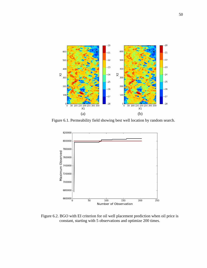
Figure 6.2 shows the evolution of the current best observed NPV as a function of the

number of PDE evaluations. The red line is the maximum NPV found by the random

47

search. The maximum NPV value increases in steps, and finally surpasses the best value

found by the random search. By only using 5 initial observations and optimize 100 times,

BGO method already gives considerably better results than a plain vanilla random search.

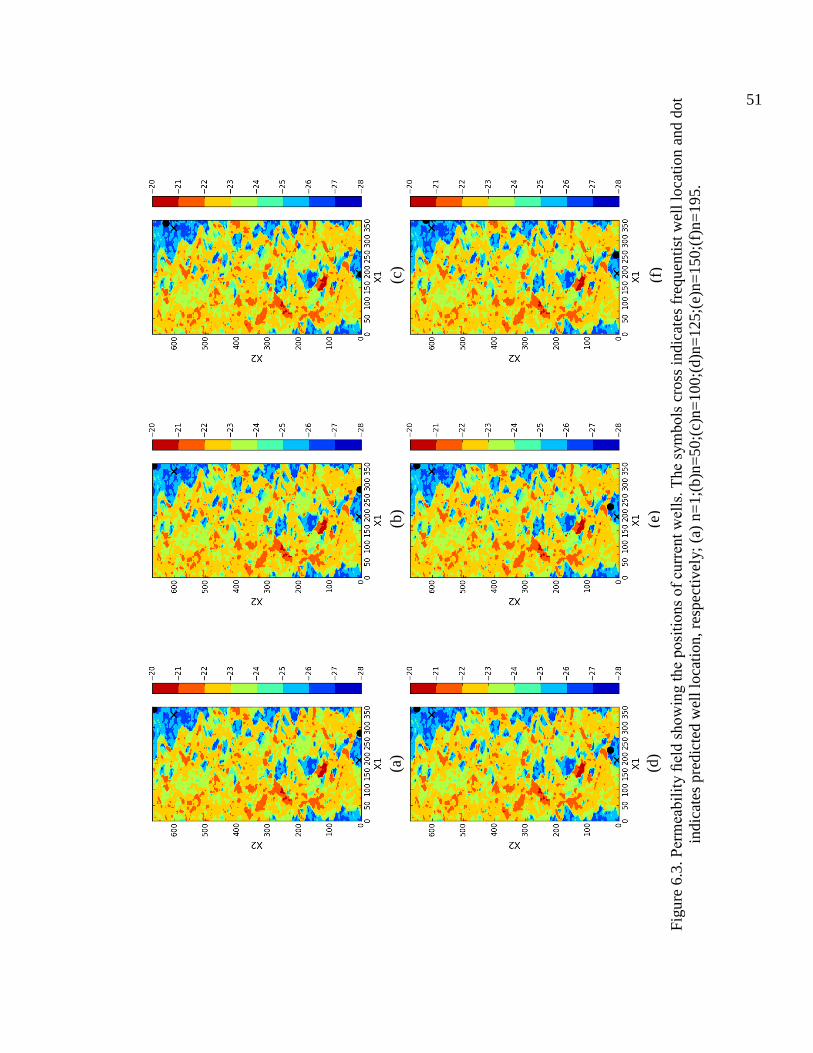
Figure 6.3 depicts the current best well location. Note that best well locations found by

BGO are close to the random search results, but not identical. It is evident, however, that

BGO finds a better solution at a fraction of the cost.

6.3 Aleatoric Uncertainty Existing in Oil Price

We now consider the case in which the NPV depends on an uncertain oil price.

Specifically, our optimization problem becomes:

(6.2)

where ( )f x is the noisy form of Equation (3.1) based on assumption ( ) ( , )o oc t c t .

In practice, when making the investment decision, we should not only aim to

maximize the expectation but also minimize the risk associated with NPV.

Mathematically, we would like to maximize the expectation of NPV while minimizing its

variance. Intuitively, more risk always leads to larger expected reward, i.e., these two

objectives are negative correlated. This multiple objective optimization can be addressed

by employing the Pareto front concept. In order to quantitatively find the trade-off

between expectation and uncertainty, we create the Figure 6.4 to visually check the result

by random search. In Figure 6.4, if we draw a line that can cover all the blue dots in the

figure, then this line is called Pareto Front line. Pareto front line represents the best

achievable trade-off between expectation and variance.

Note that we computed the variance of the NPV using the following formula:

48

1 , 1

2

1

2

1 1

2

1 1

( ) ( ) ( ) ( , )

( ) ( ) ( ) ( ) ( , )

( ) ( ) 2 ( ) ( ) ( , )

( ) ( ) 2 ( ) ( ) ( , ),

N N

i i i j i ji i j

N

i i i j i ji i j

N

i i i j i ji i j N

N

i i i j i ji i j N

Var y x P y x y x Cov P P

y x Var P y x y x Cov P P

y x Var P y x y x Cov P P

y x Var P y x y x Cov P P

(6.3)

where ( )iy x stands for the oil production rate for day i .

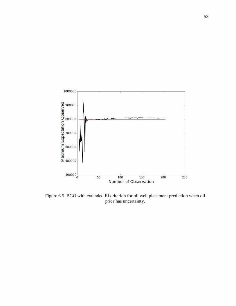
To solve the noisy optimization problem, we employ the extended EI data

acquisition policy. In Figure 6.5 we plot the evolution of the current maximum observed

projected value as a function of the number of observations. Starting with just 5 initial

random observations, we reach a solution as good as the random search after 30 iterations.

After 200 iterations of iterations, we find a solution with value about 1% larger than the

best random search value. In Figure 6.6 we show the best well locations found in this

case. They are also near the random search result, albeit not identical.

6.4 Aleatoric Uncertainty in Oil Price and Epistemic Uncertainty in Permeability

In this final example, we consider oil well placement problem with quantified

uncertainties for both the oil price and the permeability. The design optimization problem

we have to solve is: *x :

(6.4)

where the oil price is as before and K represents uncertain permeability. We apply the

BGO approach using the extended version of the EI to this problem.

49

Figure 6.7 depicts the evolution of the current observed projected maximum as a

function of the number of observations. Convergence is slower than before, albeit steady.

The spikes are due to the discounts on the Bayesian formalism induced by the fact that

the underlying GP is trained via maximum likelihood. Figure 6.8 shows the best well

location that the algorithm discovers. Comparing the results in Figure 6.8 and Figure 6.6,

we see that epistemic uncertainty in permeability brings makes BGO to require more

iterations in order to converge.

We end this section by studying the uncertainty of the NPV for a fixed well location

via Monte Carlo. Specifically, we take 1,000 joint samples of all uncertain quantities, and

compute the NPV for each sample. Then, we construct the histogram of the net present

value. Figure 6.9 depicts the result we obtain for two scenaria: 1) uncertain oil price; 2)

uncertain oil price and permeability. We can see the variance for latter case is much

larger than that in former. This is expected, for more uncertainty should bring more

variance. Notice that the mean values of two test cases are different, with the mean of the

second scenario being significantly smaller than the mean of the first scenario. A more

detailed uncertainty propagation technique would require state-of-the-art methodologies.

We refer the reader to the extensive literature.[7-9, 17]

50

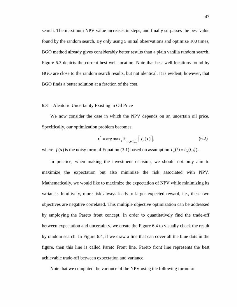
Figure 6.1. Permeability field showing best well location by random search.

Figure 6.2. BGO with EI criterion for oil well placement prediction when oil price is constant, starting with 5 observations and optimize 200 times.

(a) (b)

51

Figu

re 6

.3.

cros

s in

dica

tes

freq

uent

ist w

ell l

ocat

ion

and

dot

indi

cate

s pr

edic

ted

wel

l loc

atio

n, r

espe

ctiv

ely;

(a)

n=

1;(b

)n=

50;(

c)n=

100;

(d)n

=125

;(e)

n=15

0;(f

)n=

195.

(a)

(b)

(c)

(d)

(e)

(f)

51

52

Figure 6.4. Pareto Font line for NPV when oil price has uncertainty.

53

Figure 6.5. BGO with extended EI criterion for oil well placement prediction when oil price has uncertainty.

54

Figu

re 6

.6.

cros

s in

dica

tes

wel

l loc

atio

n gi

ven

by s

ampl

ing

and

dot i

ndic

ates

pre

dict

ed w

ell l

ocat

ion

resp

ecti

vely

; (a)

n=1;

(b)n

=10;

(c)n

=30

;(d)

n=50

;(e)

n=10

0;(f

)n=

150;

(g)n

=17

5;(h

)n=

194.

(a)

(b)

(c)

(h)

(e)

(f)

(d)

(g)

54

55

Figure 6.7. BGO with extended EI criterion for oil well placement prediction when oil price and permeability has uncertainty.

56

Figu

re 6

.8.

cros

s in

dica

tes

wel

l loc

atio

n gi

ven

by s

ampl

ing

and

dot i

ndic

ates

pre

dict

ed w

ell l

ocat

ion;

(a)

n=1;

(b)n

=50

;(c)

n=20

0;(d

)n=

300;

(e)n

=400

;(f)

n=45

0;(g

)n=

475;

(h)n

=50

0.

(a)

(b)

(c)

(h)

(e)

(f)

(d)

(g)

56

57

Figure 6.9. Histogram of net present value with 1000 samples. Green histogram line: oil price and permeability are both uncertain; Blue histogram: only oil price is uncertain.

58

CHAPTER 7. SUMMARY

The purpose of this study is to employ the machinery of BGO for design

optimization under uncertainty with limited data-budget in applications of well-

placement problem in oil-reservoir modeling. BGO uses GPR to represent our state of

knowledge and adaptively select simulation according to extended EI policy.

The mathematic background of GPR and derivation of formula for EI data-

acquisition criterion is given in previous chapter. By testing standard functions such has

Sasena, Harmant 3 and Harmant 6, proposed extended EI data acquisition is proved can

successfully approach to global maximum and minimum when there is noise in

observations, which we refer as uncertainty in this study.

Then, exact same method is used to find the best well location under three different

circumstances. No uncertainty, uncertainty in oil price and uncertainty in both oil price

and permeability. According to results shown in Chapter 6, it is proved that BGO with

extended EI policy is successfully applied in design optimization under uncertainty with

limited data-budget with applications to the well-placement problem in oil-reservoir

modeling by saving cost and improving the computing efficiency.

A big issue neglected in this study is the formulation of stopping criterion, so for

future work formulation of stopping criteria for data-acquisition process is worth

exploration. With a proper stopping standard, more budgets can be saved and

59

performance of BGO will be guaranteed. In Sec.6.3, the best well location we finally

picked out is the top one in pareto front. The risk for this point is highest, in reality, we

may seldom choose. So multiple conflicting optimization problem is also worth

exploration.

60

LIST OF REFERENCES

60

LIST OF REFERENCES

[1] Aarnes, J. E., Gimse, T., & Lie, K. A. (2007). An introduction to the numerics of flow in porous media using Matlab. In Geometric modelling, numerical simulation, and optimization (pp. 265-306). Springer Berlin Heidelberg.

[2] Arbogast, T. (2003). An overview of subgrid upscaling for elliptic problems in mixed form. Contemporary Mathematics, 329, 21-32.

[3] Arbogast, T. (2004). Analysis of a two-scale, locally conservative subgrid upscaling for elliptic problems. SIAM Journal on Numerical Analysis, 42(2), 576-598.

[4] Bangerth, W., Klie, H., Wheeler, M. F., Stoffa, P. L., & Sen, M. K. (2006). On optimization algorithms for the reservoir oil well placement problem.Computational Geosciences, 10(3), 303-319.

[5] Barker, J. W., & Thibeau, S. (1997). A critical review of the use of pseudorelative permeabilities for upscaling. SPE Reservoir Engineering, 12(2), 138-143.

[6] Beckner, B. L., & Xong, X. (1995). Field development planning using simulated annealing-optimal economic well scheduling and placement (No. CONF-951002). Society of Petroleum Engineers (SPE), Inc., Dallas, TX (United States).

[7] Bilionis, I., & Zabaras, N. (2012). Multidimensional adaptive relevance vector machines for uncertainty quantification. SIAM Journal on Scientific Computing,34(6), B881-B908.

[8] Bilionis, I., & Zabaras, N. (2012). Multi-output local Gaussian process regression: Applications to uncertainty quantification. Journal of Computational Physics, 231(17), 5718-5746.

[9] Bilionis, I., Zabaras, N., Konomi, B. A., & Lin, G. (2013). Multi-output separable Gaussian process: Towards an efficient, fully Bayesian paradigm for uncertainty quantification. Journal of Computational Physics, 241, 212-239.

[10] Bilionis, I., & Zabaras, N. (2014). Solution of inverse problems with limited forward solver evaluations: a Bayesian perspective. Inverse Problems, 30(1), 015004.

[11] Bilionis, I. py-design: Design of Experiments in Python. 2014; Available from: https://github.com/ebilionis/py-design.

[12] Bilionis, I., Drewniak, B. A., & Constantinescu, E. M. (2015). Crop physiology calibration in the CLM. Geoscientific Model Development, 8(4), 1071-1083.

[13] Bittencourt, A. C., & Horne, R. N. (1997). Reservoir development and design optimization. paper SPE, 38895, 5-8.

60

[14] Byrd, R. H., Lu, P., Nocedal, J., & Zhu, C. (1995). A limited memory algorithm for bound constrained optimization. SIAM Journal on Scientific Computing,16(5), 1190-1208.

[15] Centilmen, A., Ertekin, T., & Grader, A. S. (1999). Applications of neural-networks in multi-well field development (Doctoral dissertation, Pennsylvania State University).

[16] Chaudhuri, A., Haftka, R., & Viana, F. (2012, April). Efficient Global Optimization with Adaptive Target for Probability of Targeted Improvement. In8th AIAA Multidisciplinary Design Optimization Specialist Conference, American Institute of Aeronautics and Astronautics, Honolulu, HI (pp. 1-13).

[17] Chen, P., Zabaras, N., & Bilionis, I. (2015). Uncertainty propagation using infinite mixture of Gaussian processes and variational Bayesian inference.Journal of Computational Physics, 284, 291-333.

[18] Chen, Z., & Hou, T. (2003). A mixed multiscale finite element method for elliptic problems with oscillating coefficients. Mathematics of Computation,72(242), 541-576.

[19] Chen, Z., Huan, G., & Ma, Y. (2006). Computational methods for multiphase flows in porous medi (Vol. 2). Siam.

[20] Christie, M. A. (1996). Upscaling for reservoir simulation. Journal of Petroleum Technology, 48(11), 1-004.

[21] Christie, M. A., & Blunt, M. J. (2001). Tenth SPE comparative solution project: A comparison of upscaling techniques. SPE Reservoir Evaluation & Engineering, 4(04), 308-317.

[22] Demond, A. H., & Roberts, P. V. (1987). An examination of relative permeability relations for two-phase flow in porous media. JAWRA Journal of the American Water Resources Association,23(4), 617-628.

[23] Elamvazuthi, I., Vasant, P., & Ganesan, T. (2013). Hybrid optimization techniques for optimization in a fuzzy environment. In Handbook of Optimization (pp. 1025-1046). Springer Berlin Heidelberg.

[24] Ghanem, R. G., & Spanos, P. D. (2003). Stochastic finite elements: a spectral approach. Courier Corporation.

[25] Güyagüler, B., & Horne, R. N. (2004). Uncertainty assessment of well-placement optimization. SPE Reservoir Evaluation & Engineering, 7(01), 24-32.

[26] Hedar, A. R. (2013). Global optimization test problems. URL http://www-optima. amp. i. kyoto-u. ac. jp/member/student/hedar/Hedar_files/TestGO. htm.

[27] Honarpour, M., & Mahmood, S. M. (1988). Relative-permeability measurements: An overview. Journal of petroleum technology, 40(08), 963-966.

[28] Hou, T. Y., & Wu, X. H. (1997). A multiscale finite element method for elliptic problems in composite materials and porous media. Journal of computational physics, 134(1), 169-189

[29] Inman, R. L., Helson, J. C., & Campbell, J. E. (1981). An approach to sensitivity analysis of computer models: Part II-ranking of input variables, response surface validation, distribution effect and technique synopsis. Journal of Quality Technology, 13(4).

61

[30] Jones, D. R., Schonlau, M., & Welch, W. J. (1998). Efficient global optimization of expensive black-box functions. Journal of Global optimization,13(4), 455-492

[31] Jones, D. R. (2001). A taxonomy of global optimization methods based on response surfaces. Journal of global optimization, 21(4), 345-383.

[32] Lawrence, D. B. (1999). The economic value of information. Springer. [33] Lázaro-Gredilla, M., Quiñonero-Candela, J., Rasmussen, C. E., & Figueiras-Vidal,

A. R. (2010). Sparse spectrum Gaussian process regression. The Journal of Machine Learning Research, 11, 1865-1881.

[34] Maini, B. B., & Okazawa, T. (1987). Effects of temperature on heavy oil-water relative permeability of sand. J. Cdn. Pet. Tech.(May-June 1987), 33-41.

[35] Marek, C., & Tomasz, Z. (2011). Mathematics for Finance-An Introduction to Financial Engineering.

[36] Mattax, C. C., & Dalton, R. L. (1990). Reservoir simulation. [37] Mockus, J., Tiesis, V., & Zilinskas, A. (1978). The application of Bayesian

methods for seeking the extremum. Towards Global Optimization, 2(117-129), 2. [38] Pardalos, P. M., & Resende, M. G. (Eds.). (2001). Handbook of applied

optimization. Oxford university press. [39] Powell, W. B., & Ryzhov, I. O. (2012). Optimal learning (Vol. 841). John Wiley

& Sons. [40] Pride, S. R., Harris, J. M., Johnson, D. L., Mateeva, A., Nihel, K. T., Nowack, R.

L., ... & Fehler, M. (2003). Permeability dependence of seismic amplitudes.The Leading Edge, 22(6), 518-525.

[41] Renard, P., & De Marsily, G. (1997). Calculating equivalent permeability: a review. Advances in Water Resources, 20(5), 253-278.

[42] Smith, T. E., & Dearmon, J. (2014). Gaussian Process Regression and Bayesian Model Averaging: An alternative approach to modeling spatial phenomena.

[43] Spall, J. C. (2005). Introduction to stochastic search and optimization: estimation, simulation, and control (Vol. 65). John Wiley & Sons.

[44] Zheng, S. Y., Corbett, P. W., Ryseth, A., & Stewart, G. (2000). Uncertainty in well test and core permeability analysis: a case study in fluvial channel reservoirs, northern North Sea, Norway. AAPG bulletin, 84(12), 1929-1954.