Bayesian estimation methods for contingency tables

J. ltal. Statist. Soc. (1993) 1, pp. 35-54

B A Y E S I A N ESTIMATION M E T H O D S F O R C O N T I N G E N C Y T A B L E S

Constantinos Goutis University College London

Summary

A method of inputting prior opinion in contingency tables is described. The method can be used to incorporate beliefs of independence or symmetry but extensions are straightforward. Logistic normal distributions that express such beliefs are used as priors of the cell probabilities and posterior estimates are derived. Empirical Bayes methods are also discussed and approximate posterior variances are provided. The methods are illustrated by a numerical example.

Keywords: Logistic normal distribution, Empirical Bayes methods, independence, symmetry.

1. Introduction

Suppose that data are collected and cross-classified with respect to two or more categorical variables. Consider the random vector of cell counts, arranged in a contingency table, having a multinomial or a product multinomial distribution. The usual frequentist approach (McCullagh and Nelder 1989, Bishop, Fienberg and Holland 1975) postulates a model, often having an interpretation in terms of (conditional) independence or symmetry, and calculates the estimates of cell probabilities using maximum likelihood estimation. A goodness of fit test (using statistics such as Pearson's X 2 or the deviance G 2) is used to determine if the estimates are acceptable.

It may happen that the practitioner has some prior information about the proportion of the data in each category and about the pattern that the proportion follow. In that case a Bayesian approach may be desirable. Unsurpri- singly the problem of how to input prior information has a long history. Ear- lier work includes Lindley (1964), Altham (1969) and Leonard (1972, 1975). One way is to assume that the probabilities possess a Dirichlet conjugate prior distribution. The Dirichlet density accepts parameters interpretable as prior guesses of the means of cell probabilities and one additional precision parameter. However it has many strong independence properties, in the sense that essentially the only covariance structure that exists between the components of a Dirichlet distributed vector is due to the fact that they add

35

C . G O U T I S

to one (see a.g. Aitchison 1982, 1986), so it may be hard to incorporate separate prior knowledge about, say, independence or some other feature of prior beliefs. Furthermore it has a single precision parameter, not allowing varying degrees of uncertainty in the prior cell means. Solutions to this problem include the use of mixtures of Dirichlet distributions [Albert and Gupta (1982, 1983a), Albert (1985), Good (1976), Crook and Good (1980), Leonard and Novick (1986), Gupta, Saleh and Sen (1989)] or priors on functions of cell probabilities (Albert and Gupta 1983b).

An alternative approach is to specify a model for the cell probabilities and then introduce uncertainty by assuming that the parameters of the model are distributed according to some (usually hierarchical) prior. The method can be viewed as a generalisation of Lindley and Smith (1972) and has been used for contingency tables by Leonard (1975), whose work was extended for higher order tables by Nazaret (1987). A similar approach was adopted by Albert (1988) whereas Laird (1978) and Piegorsch and Casella (1990) used empirical Bayes methods based on the same idea. However parameters of generalised linear models such as multivariate logits are not easily interpretable, so it might be difficult to incorporate prior knowledge through them. It may be preferable to use a prior directly on the cell probabilities.

Apart from the Dirichlet distribution, another useful and richer class is the logistic normal distribution, studied by Aitchison and Shen (1980), who give further references on its use. As we will see in the following, the logistic normal has more parameters than the Dirichlet distribution and can model dependence structures easier, since, compared with Dirichlet, it allows different precisions and more complicated covariance structures of the components of a random variable. In Bayesian statistics it has appeared as an approximation to posterior distributions (Lindley 1964, Bloch and Watson 1967) but, somehow curiously and despite Aitchison's (1985a) speculation, it seems to be absent when trying to incorporate prior knowledge, Leonard (1972) being an exception. It has also been used by Leonard (1973) in a related problem of smoothing the probabilities in a histogram. We first give the de- finition and a derivation and some properties that we will need. For further details see Aitchison and Shen (1980) or Aitchison (1986).

Suppose that X = (2(1, 2(2, ..., Xa) follows a multivariate lognormal distribution Aa (~,~12). Then the composition of X, defined by P = (Pz, P2,

d ~

---, Pa) where Pi = Xi/( .E Xj), follows a logistic normal distribution La (14

Z), with density function

1 exp[ - 1 d 7 {log(pd-1/pd.) --#} r 2--1 {log(pd--1/pd.) --#}l (1.1)

36

BAYESIAN ESTIMATION METHODS

d where pa_l = (Pl, P2 . . . . . Pa -1 ) , forpi > 0, 27 Pi = 1. T h e parameters (#, 27)

are given by/~ = A~ and Z = AD.A r where A = [ I - / ], I is the identity matrix and I iffa veci'or of ones of the appropriate order. Note that, as Dawid (1982) pointed out, @ s determine (/A Z) but not conversely; we can re- place ~ by ~ + c and 12 by s + 1 6 r + "6 1 r for any constant c and vector 6. Thougla no"/obvious, there is nop'refereniial treatment for Pd, in the sense that a permutation of subscripts yields a different form of density and different parameters (/A Z) but not different values of the density or distribution functions. Alternative parameterisations in terms of multivariate logits or successive logcontrasts exist and may prove useful in some contexts (see Aithison i982). A more symmetric form of the density, given by Aitchison (1985b), is proportional to

exp i= (rpi - 1 ) log pi - 2

where X --1 = [ r J ,

~q ( log Pi - log p])2 (1.2) j=/.i= l

1 ~oq = - -ff- rq ( i 4 = j = 1 , 2 . . . . . d - l ) , (1.3)

1 d--1 . . . . X rij ( i = 1 , 2 , d - 1), (1.4) ~l) di ~id 2 ]=1 .. . .

d - I

r = ~--1/4 q0a = - ~ ' q)i and cPa-1 = (rPl, cP2 . . . . , q)a-1). (1.5)

Formula (1.2) can be considered as the kernel of a more general distribution a

function, in the sense that ,~' qgi = 0 need not hold. If ~pq = 0, it degenerates i=l

to a Dirichlet distribution, so the density (1.2), in its general form, has both Dirichlet and logistic normal densities as special cases.

We will use the term s u b c o m p o s i t i o n for the composition of a subvector of p or X. Note that the subcompositions of p or X corresponding to the same "ffubsc~pts are identical and have a logis'tic normal distribution with the appropriate parameters. It is interesting to note that the Dirichlet distribution can be derived as the distribution of the composition of independent gamma random variables, with the same scale parameter and this implies strong independence properties for Dirichlet (Aitchison 1982, 1986).

We chose to model prior information through logistic normal distributions for the following reasons:

(i) It is possible to specify a prior distribution directly on cell probabilities or

37

C. GOUTIS

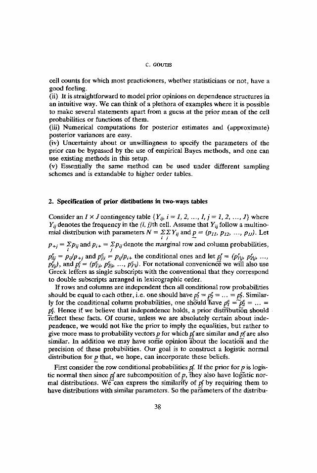
cell counts for which most practicioners, whether statisticians or not, have a good feeling. (ii) It is straightforward to model prior opinions on dependence structures in an intuitive way. We can think of a plethora of examples where it is possible to make several statements apart from a guess at the prior mean of the cell probabilities or functions of them. (iii) Numerical computations for posterior estimates and (approximate) posterior variances are easy. (iv) Uncertainty about or unwillingness to specify the parameters of the prior can be bypassed by the use of empirical Bayes methods, and one can use existing methods in this setup. (v) Essentially the same method can be used under different sampling schemes and is extandable to higher order tables.

2. Specification of prior distibutions in two-ways tables

Consider an I • J contingency table { Yq, i = 1, 2 . . . . . I, j = 1, 2, . . . , J} where Yij denotes the frequency in the (i, j ) th cell. Assume that Yij follow a multinomial distribution with parameters N = X . ~ Y q and p = (Plx, P12, . . . , PIJ). Let

p+j = ~iPiJ and Pi+ = ~.Pq denote the marginal row and column probabilities, /

Pfli = Pi /P +j and P~i = Pi/Pi+ the conditional ones and le t /~ = (P~[i, PSlj, .. . . P~ti), and p~ = (P~[i, P~li, . . . , P~rg" For notational convenienc~ we will also use Greek leffers as single subscripts with the conventional that they correspond to double subscripts arranged in lexicographic order.

If rows and columns are independent then all conditional row probabilities should be equal to each other, i.e. one should have p~ = P5 = ... = P~. Similar- ly for the conditional column probabilities, one should ]lave p~ --"p~ -- ... = p~. Hence if we believe that independence holds, a prior dist~buti 'rn should ~'eflect these facts. Of course, unless we are absolutely certain about independence, we would not like the prior to imply the equalities, but rather to give more mass to probability vectors p for which/~are similar and p~ are also similar. In addition we may have sor~e opinion a-'bout the locatio~ and the precision of these probabilities. Our goal is to construct a logistic normal distribution for p that, we hope, can incorporate these beliefs.

First consider the row conditional probabilities/~. If the prior for p is logistic normal then since/~rare subcomposition of p, t-'hey also have logq'stic normal distributions. W~'can express the similarity of p~ by requiring them to have distributions with similar parameters. So the pa~mete r s of the distribu-

38

BAYESIAN ESTIMATION M E T H O D S

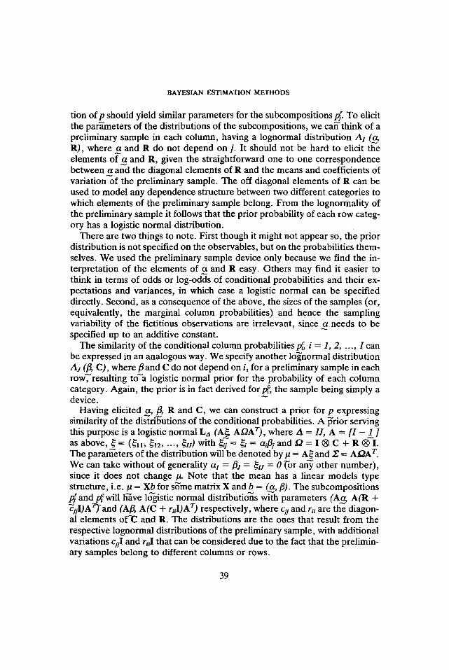
tion of p should yield similar parameters for the subcompositions/~. To elicit the parameters of the distributions of the subcompositions, we ca~'think of a preliminary sample in each column, having a lognormal distribution Az (~ R), where a and R do not depend on j. It should not be hard to elicit the elements of"a and R, given the straightforward one to one correspondence between a and the diagonal elements of R and the means and coefficients of variation of the preliminary sample. The off diagonal elements of R can be used to model any dependence structure between two different categories to which elements of the preliminary sample belong. From the lognormality of the preliminary sample it follows that the prior probability of each row category has a logistic normal distribution.

There are two things to note. First though it might not appear so, the prior distribution is not specified on the observables, but on the probabilities them- selves. We used the preliminary sample device only because we find the interpretation of the elements of ~ and R easy. Others may find it easier to think in terms of odds or log-odds of conditional probabilities and their expectations and variances, in which case a logistic normal can be specified directly. Second, as a consequence of the above, the sizes of the samples (or, equivalently, the marginal column probabilities) and hence the sampling variability of the fictitious observations are irrelevant, since ct needs to be specified up to an additive constant.

The similarity of the conditional column probabilities p~, i = 1, 2 . . . . . I can be expressed in an analogous way. We specify another lo~normal distribution Aj (/~ C), where fl and C do not depend on i, for a preliminary sample in each row, resulting t r ' a logistic normal prior for the probability of each column category. Again, the prior is in fact derived for pi r the sample being simply a device.

Having elicited a, fl, R and C, we can construct a prior for p expressing similarity of the di~fi~utions of the conditional probabilities. A ~'rior serving this purpose is a logistic normal L,a (A~ AK2Ar), where A = I J, A = [I - 1 ] as above, ~ = (~11 , ~12 . . . . . ~lJ) with ~/7 = ~i = ctiflj and ~2 = I | C + R | I. The paratrTeters of the distribution will be denoted by # = A~and ~ = A~2A r. We can take without of generality al = flj = ~H = 0 ('or any other number), since it does not change /~ Note that the mean has a linear models type structure, i.e. # = Xb for s~'me matrix X and b = (a,/~). The subcompositions ~ a n d p~will have lo"gistic normal distributions with parameters (A~ A(R + ~jI)Ar)'and (Aft, A(C + riiI)A r) respectively, where cjj and rii are the diagonal elements of"C and R. The distributions are the ones that result from the respective lognormal distributions of the preliminary sample, with additional variations cjjI and riJ that can be considered due to the fact that the preliminary samples belong to different columns or rows.

39

C. GOUTIS

Perhaps not surprisingly, the form of the prior mean of logpij is similar to the form of log Pij under an independence log-linear model but there is also a variance covariance structure. Note that out approach is different from the one of Leonard (1975) in that we assume that pq follow a distribution, not the vectors ..a and/3. Leonard's approach considers Pij deterministic functions of a and fl and speEifies the prior on them. Hence in his approach, for any a and fl the ffrobabilities have an a priori an independence structure, that is, the prio-f is concentrated on the set `9 = (p ] Pij = Pi+P+j for some Pi+ and p+j}. There is a prior uncertainty about the'~alues of the marginals p;+ and p+j which is expressed in the distribution of a and ft. In our approach, not all prior mass is concentrated on the set `9, unless the'prior variance covariance matrices are degeneate. Instead, our priors give more weight to probabilities pq that are <<close>> to .9 in some sense, and the prior variance covariance matrices indicate a way of expressing this proximity. Of course one could use a two-stage hierarchical prior on p I a , fl and marginally on a , fl but, as will see, it is not advisable to do so.

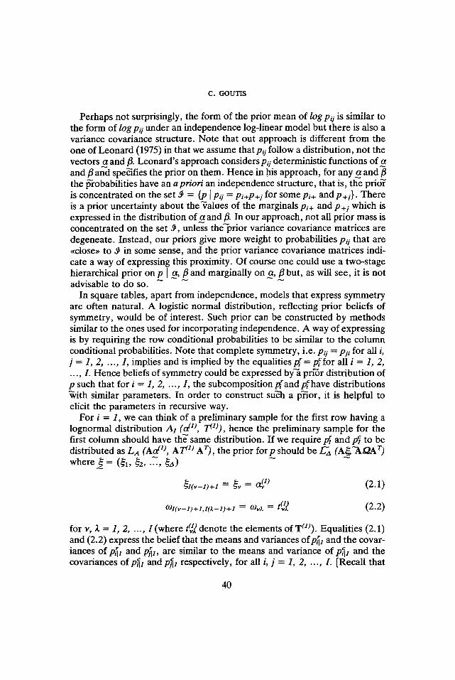
In square tables, apart from independence, models that express symmetry are often natural. A logistic normal distribution, reflecting prior beliefs of symmetry, would be of interest. Such prior can be constructed by methods similar to the ones used for incorporating independence. A way of expressing is by requiring the row conditional probabilities to be similar to the column conditional probabilities. Note that complete symmetry, i.e. pq = Pii for all i, j = 1, 2 . . . . . I, implies and is implied by the equalities p [= pTfor all i = 1, 2, .... I. Hence beliefs of symmetry could be expressed by~ pn~r distribution of p such that for i = 1, 2 . . . . . I, the subcomposition p~and pfhave distributions ~,ith similar parameters. In order to construct suc-'h a p~or, it is helpful to elicit the parameters in recursive way.

For i = 1, we can think of a preliminary sample for the first row having a lognormal distribution Ax (d 1), Tel)), hence the preliminary sample for the first column should have the" same distribution. If we require p~ and p~ to be distributed as LA (Act (I), AT (1) AT), the prior fo rp should be ffa (A~ "~AK2A r) w h e r e ~ = (~1, ~2,--~-, ~a) ~

~ 1 ( v - 1 ) + 1 = ~v = Or(l) (2.1)

( 1 ) l ( v _ l ) + l , l O _ l ) + l = (gv) " = t~] (2.2)

for v, A = 1, 2, ..., I (where t~;~ denote the elements of T(1)). Equalities (2.1) and (2.2) express the belief that the means and variances o fp~/and the covariances of P~I and P~1, are similar to the means and variance of P~I and the covariances of P~I and P~I respectively, for all i, j = 1, 2, ..., I. [Recall that

40


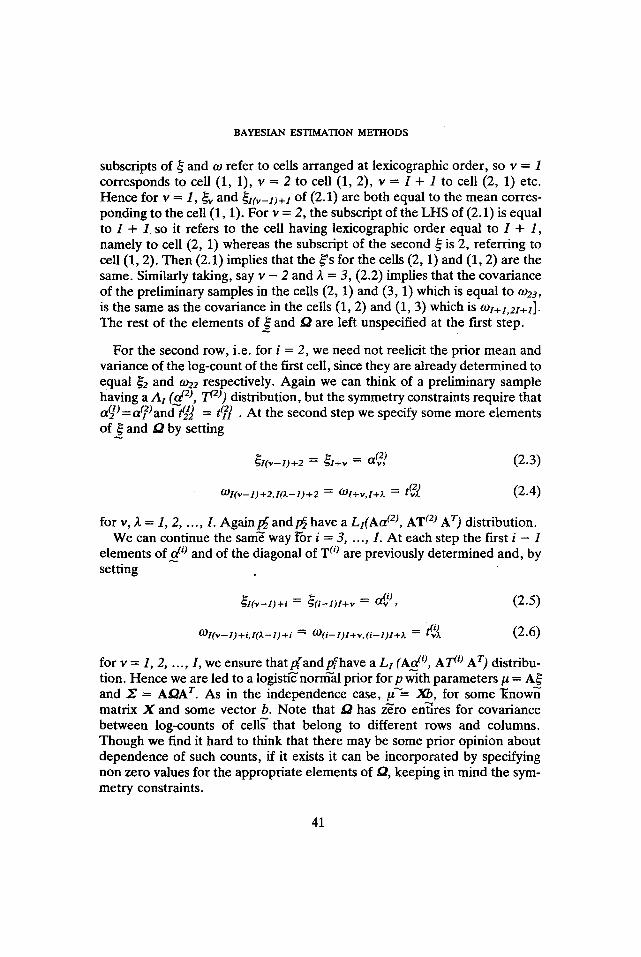
subscripts of ~ and to refer to cells arranged at lexicographic order, so v = 1 corresponds to cell (1, 1), v = 2 to cell (1, 2), v = I + 1 to cell (2, 1) etc. Hence for v = 1, ~,, and ~i0,-1)+1 of (2.1) are both equal to the mean corresponding to the cell (1, 1). For v = 2, the subscript of the LHS of (2.1) is equal to I + 1 so it refers to the cell having lexicographic order equal to I + 1, namely to cell (2, 1) whereas the subscript of the second ~ is 2, referring to cell (1, 2). Then (2.1) implies that the ~'s for the cells (2, 1) and (1, 2) are the same. Similarly taking, say v - 2 and ,~ = 3, (2.2) implies that the covariance of the preliminary samples in the cells (2, 1) and (3, 1) which is equal to to23, is the same as the covariance in the cells (1, 2) and (1, 3) which is toI+l ,21+l]" The rest of the elements of ~ and 12 are left unspecified at the first step.

For the second row, i.e. for i = 2, we need not reelicit the prior mean and variance of the log-count of the first cell, since they are already determined to equal ~2 and to22 respectively. Again we can think of a preliminary sample having a At (a 12), T c2)) distribution, but the symmetry constraints require that

(O (2) ~ 1 a2 = a l and ~ = t(12] . At the second step we specify some more elements o f ~ and 12 by setting

~/(~-1)+2 = ~l+~ = a~, ) (2.3)

tol(v--1)+2,1(~--l)+2 = O)l+v,l+Z = t ~ (2.4)

for v, 2 = 1, 2 . . . . . I. Again p~ andp~ have a Zl(ACt (2), AT (2) A T) distribution. We can continue the sam~ way t'or i = 3 . . . . . I. At each step the first i - 1

elements o f d ~ and of the diagonal of T (~ are previously determined and, by setting

~I(v- - l )+i : ~( i--1) l+v = a(~ ) , (2.5)

O)l(v_l)+i , lO ._ l )+ i ~- ( .O( i_ l ) l+v . ( i_ l ) l+ z = t(iv)~ (2.6)

for v = 1, 2, ..., I, we ensure that p(andp~have a Lt ( A d 0, AT r0 A r) distribution. Hence we are led to a logisti'ffnorrrTal prior for p with parameters # = A~ and Z = A~A r. As in the independence case, ~"= Xb, for some ~nown matrix X and some vector b. Note that 12 has z~ro ent"{res for covariance between log-counts of cells that belong to different rows and columns. Though we find it hard to think that there may be some prior opinion about dependence of such counts, if it exists it can be incorporated by specifying non zero values for the appropriate elements of 12, keeping in mind the symmetry constraints.

41

C. GOUTIS

3. Extensions

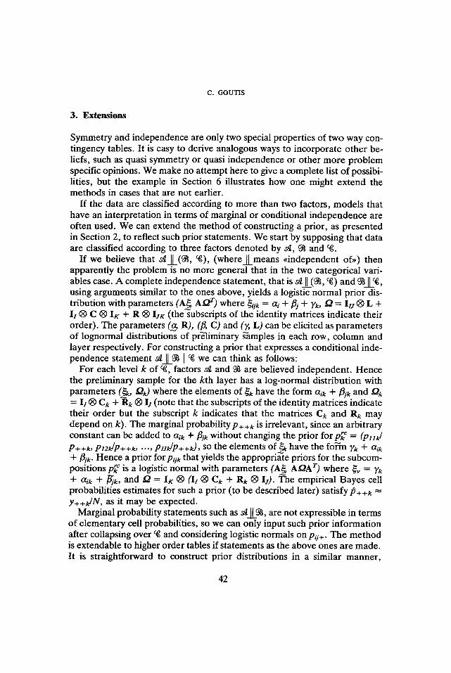
Symmetry and independence are only two special properties of two way contingency tables. It is easy to derive analogous ways to incorporate other beliefs, such as quasi symmetry or quasi independence or other more problem specific opinions. We make no attempt here to give a complete list of possibi- lities, but the example in Section 6 illustrates how one might extend the methods in cases that are not earlier.

If the data are classified according to more than two factors, models that have an interpretation in terms of marginal or conditional independence are often used. We can extend the method of constructing a prior, as presented in Section 2, to reflect such prior statements. We start by supposing that data are classified according to three factors denoted by s~, ~ and %.

If we believe that s l ~ ( ~ , ~), (where]Lmeans ~independent of,) then apparently the problem is no more general that in the two categorical variables case. A complete independence statement, that is s ~ ( ~ , %) and ~1[%, using arguments similar to the ones above, yields a logistic normal prior distribution with parameters (A~ A~2 r) where ~i/k = ai + fly + Yk, K2 = Iu | L + Ii @ C | I r + R | I j r (the'subscripts of the identity matrices indicate their order). The parameters (~ R), (fl, C) and (7, L) can be elicited as parameters of lognormal distributions of pre-'liminary ~mples in each row, column and layer respectively. For constructing a prior that expresses a conditional independence statement ,~_~_~ 1% we can think as follows:

For each level k of %, factors si and ~ are believed independent. Hence the preliminary sample for the kth layer has a log-normal distribution with parameters (~k, Qk) where the elements of ~k have the form aik dr fljk and ~'~k = Ii | Ck dr Rk | Ij (note that the subscripts of the identity matrices indicate their order but the subscript k indicates that the matrices Ck and R k may depend on k). The marginal probability P++k is irrelevant, since an arbitrary constant can be added to ~lik dr fljk without changing the prior for p~C = (Pile~ P++k, P l 2 k / P + + k , . . . . Puk/P++k), SO the elements of ~k have the fo~rn Yk + Ctik + flit,- Hence a prior for pijt` that yields the appropriff'te priors for the subcompositions p~C is a logistic normal with parameters (A~, AQA r) where ~,, = ),t, dr Glik dr ffjk, and t2 = I r | (Ii | Ct, + R k ~ Ij). "Fhe empirical Bayes cell probabilities estimates for such a prior (to be described later) satisfy 10++k y++k/N, as it may be expected.

Marginal probability statements such as ~ _ ~ , are not expressible in terms of elementary cell probabilities, so we can only input such prior information after collapsing over ~ and considering logistic normals on P~i+" The method is extendable to higher order tables if statements as the above ones are made. It is straightforward to construct prior distributions in a similar manner,

42

BAYESIAN E S T I M A T I O N M E T H O D S

though as the number of factors increases, so does the number of possible independence and conditional independence statements that can be made.

Different sampling methods can be accommodated, and, indeed, the problem is easier. This is essentially a generalisation of Leonard's (1973) method, and we will not describe it in detail. A product multinomial likelihood is common. In a tw0-way table, assuming without loss of generality that column marginals are fixed, we can consider an independence prior by assuming that PrO have logistic normal distributions with the same parameters. In higher order tables, we need consider only the conditional on the fixed margins probabilities.

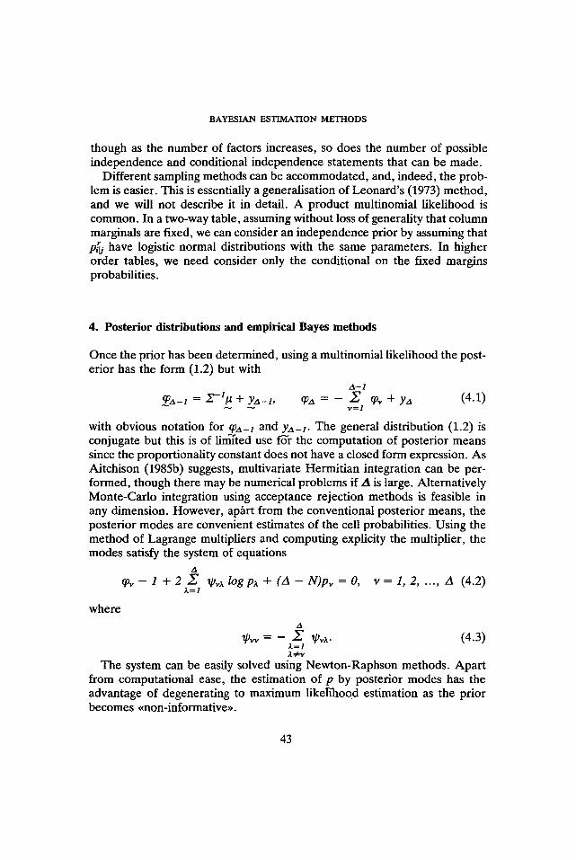
4. Posterior distributions and empirical Bayes methods

Once the prior has been determined, using a multinomial likelihood the posterior has the form (1.2) but with

A--1

~a-1 = Z - l # + Ya-l, q0a = - ~Y' qo~, + Ya (4.1) "v'=l

with obvious notation for q0a-1 and Ya-1- The general distribution (1.2) is conjugate but this is of limited use f'6"r the computation of posterior means since the proportionality constant does not have a closed form expression. As Aitchison (1985b) suggests, multivariate Hermitian integration can be per- formed, though there may be numerical problems if A is large. Alternatively Monte-Carlo integration using acceptance rejection methods is feasible in any dimension. However, ap~rt from the conventional posterior means, the posterior modes are convenient estimates of the cell probabilities. Using the method of Lagrange multipliers and computing explicity the multiplier, the modes satisfy the system of equations

where

A

cp, , - l + 2 . ~ 3.=1

~O,,x log Px + (A -- N)p~, = O, v = l , 2 . . . . . A (4.2)

A

~P~, = - ~Y' ~/'~x. (4.3) 3.=1 3.~v

The system can be easily solved using Newton-Raphson methods. Apart from computational ease, the estimation of p by posterior modes has the advantage of degenerating to maximum likelihood estimation as the prior becomes ~non-informative,>.

43

C. GOUTS

It is interesting to note that the difference between prior and posterior distribution is in the parameters cp~,, whereas ~0~x remain unchanged. The prior (and posterior) ~p~x depend entirely on the variance-covariance matrix

whereas the posterior qo,, depend on the prior/~ and ~, as well as the data. From (4.2) and (4.3) it can be seen that the postfffior estimates depend on all these quantities, but not to the same degree. As it is expected, and we will see lateron, the posterior estimates are in some sense in the between of our prior beliefs and the maximum likelihood estimates under no structure. The matrix ~determines basically the proximity of the posterior to the likelihood whereas/~ determines the direction of the deviation of the posterior modes from the-'maximum likelihood estimates.

Drawing an analogy with simpler situations, one would expect that the effect of ~ (roughly equivalent to the prior precision) on the posterior is not as dramatic as the effect of/~ (the prior location of the estimates). In that sense, the uncertainty about'~alues of ~ (hence of ~p,,x) is of less importance than the uncertainty about values of/~, unless of course the sample is very small, and a "wrong" specification o f '~ woud not have a detrimental effect. The results should be fairly robust with respect to changes of the prior ~p,,x. On the other hand the specification of/ t does have a large effect and requires some strong prior beliefs in the marginaqs of the table. If such beliefs do exist, then there should be no problems in eliciting them, however, if they do not exist, a proper Bayesian analysis may be unsatisfactory.

It is often convenient to model prior knowledge through a two stage prior; the second stage being a diffuse or non-informative prior on the parameters of the first stage prior. However in this case, we cannot get sensible results using that approach. If the parameter b has, say, a normal distribution, the effect is that p has a logistic normal distribution with larger variance covariance matrix.-We can immediately see that as the variance matrix gets large (in the sense that the eigenvalues tend to infinity) the posterior distribution tends to the likelihood function with no structure in p, hence the prior input about indepence or symmetry is lost.

As an alternative to the full Bayes analysis as described, we consider empirical Bayes methods. The approach allows some features of the prior distribution to be inferred from the data. More specifically we use parametric empirical Bayes analysis (Morris 1983), in which the form of the prior is pre- specified but the parameters of the prior are estimated from the marginal distribution of the data. The empirical Bayes method has been used in a similar way by Laird (1978), but the problem was not identical. In her setup, the goal was to estimate the cell probabilities based on combining log linear models and normal prior distributions on the parameters of the linear model. The prior that was used was Leonard's (1975) prior on the vectors of the main

44


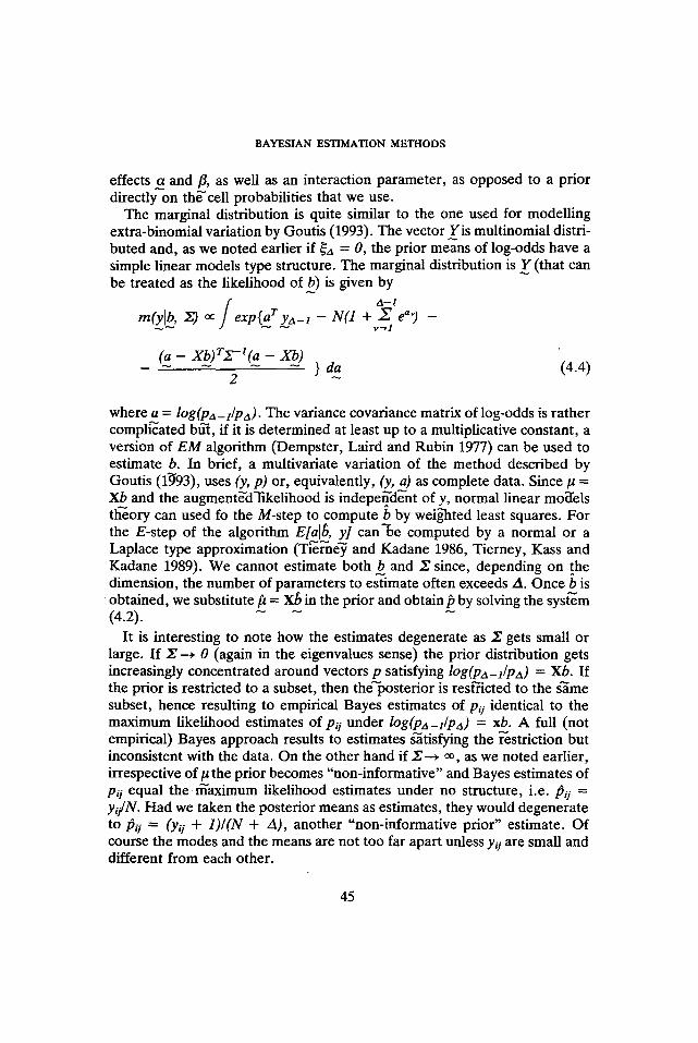
effects a and fl, as well as an interaction parameter, as opposed to a prior directly on the'cell probabilities that we use.

The marginal distribution is quite similar to the one used for modelling extra-binomial variation by Goutis (1993). The vector Yis multinomial distributed and, as we noted earlier if ~a = 0, the prior means of log-odds have a simple linear models type structure. The marginal distribution is Y (that can be treated as the likelihood of b) is given by

.4--1

m(ylb, Z) ~ exp{a.qf y`4-1 - N U + Z e a') -

2 } d a (4.4)

where a = log(pa_l/pa). The variance covariance matrix of log-odds is rather compl~ated bfii, if it is determined at least up to a multiplicative constant, a version of E M algorithm (Dempster, Laird and Rubin 1977) can be used to estimate b. In brief, a multivariate variation of the method described by Goutis (19"93), uses (y, p) or, equivalently, (y, a) as complete data. Since # = Xb and the augment~'dqikelihood is indepeffd~'nt of y, normal linear mo~els theory can used fo the M-step to compute b by weighted least squares. For the E-step of the algorithm E[a[b, y] can-be computed by a normal or a Laplace type approximation ( T ~ a e ~ and Kadane 1986, Tierney, Kass and Kadane 1989). We cannot estimate both b and Z since, depending on the dimension, the number of parameters to estimate often exceeds A. Once b is obtained, we substitute ~ = Xb in the prior and obtain t5 by solving the sysffrm (4.2). - -

It is interesting to note how the estimates degenerate as Z gets small or large. If Z ~ 0 (again in the eigenvalues sense) the prior distribution gets increasingly concentrated around vectors p satisfying log(pa_dpa) = Xb. If the prior is restricted to a subset, then the"posterior is resfficted to the s~me subset, hence resulting to empirical Bayes estimates of pq identical to the maximum likelihood estimates of pq under log(pa-dpa) = xb. A full (not empirical) Bayes approach results to estimates ~tisfying the ~striction but inconsistent with the data. On the other hand if Z--~ ~ , as we noted earlier, irrespective of # the prior becomes "non-informative" and Bayes estimates of pq equal the r~aximum likelihood estimates under no structure, i.e./~ij = yi /N. Had we taken the posterior means as estimates, they would degenerate to/~q = (Yo + 1)/(N + A), another "non-informative prior" estimate. Of course the modes and the means are not too far apart unless yq are small and different from each other.

45

C. GOUTIS

5. Approximate posterior variance

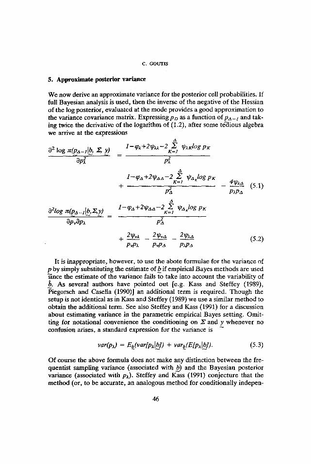
We now derive an approximate variance for the posterior cell probabilities. If full Bayesian analysis is used, then the inverse of the negative of the Hessian of the log posterior, evaluated at the mode provides a good approximation to the variance covariance matrix. Expressing Po as a function o fpa -1 and taking twice the derivative of the logarithm of (1.2), after some tedious algebra we arrive at the expressions

z~

32 log zr(pa-l~, Z, y) 1-cpx+21pxx-2 .~ ~pxKIOg pK ~-r -~- K = l

3d d A

1--q~A +2~aa--2 ~--~ ~A~lOg pr K=I 4~PXa (5.1)

+ p2 PxPa

A

02log ~r(p,~_llb, Z,y ) = 1-epa +2~paa-2K=, "~ ~pAJog PK

3p 3p

+ 2 ~P,,x 2 ~P,,zx 2~Pxa (5.2) P~Px P,,Pz~ PxPa

It is inappropriate, however, to use the abote formulae for the variance of p by simply substituting the estimate o f b if empirical Bayes methods are used ~ince the estimate of the variance fails to take into account the variability of b. As several authors have pointed out [e.g. Kass and Steffey (1989), "Piegorsch and Casella (1990)] an additional term is required. Though the setup is not identical as in Kass and Steffey (1989) we use a similar method to obtain the additional term. See also Steffey and Kass (1991) for a discussion about estimating variance in the parametric empirical Bayes setting. Omit- ting for notational convenience the conditioning on 27 and y whenever no confusion arises, a standard expression for the variance is

var(px) = Eb.(var[pxlb]) + var~(E[pxlb]). (5.3)

Of course the above formula does not make any distinction between the frequentist sampling variance (associated with b b ) and the Bayesian posterior variance (associated with Px)- Steffey and Kass (1991) conjecture that the method (or, to be accurate, an analogous method for conditionally indepen-

46


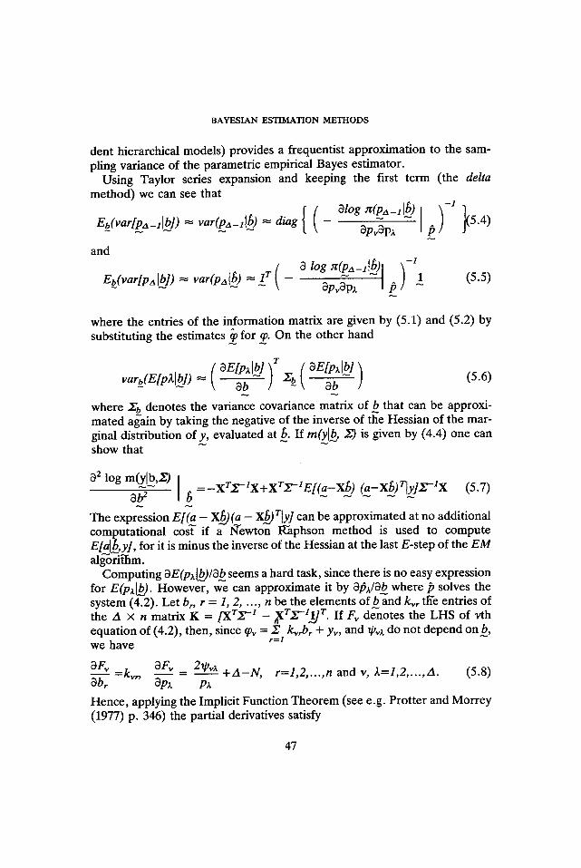
dent hierarchical models) provides a frequentist approximation to the sam- piing variance of the parametric empirical Bayes estimator.

Using Taylor series expansion and keeping the first term (the delta method) we can see that

-1

Eb(var[pa-,lb]) ~- var(pa-llb) -~ diag - Op~ap~ p

and

Eb(var[palb]) ~ var(pAl~) ~- 1 r [\ _ 2 log :t(Pa-l[~) I1 (5.5)

where the entries of the information matrix are given by (5.1) and (5.2) by substituting the estimates ~ for ~. On the other hand

Oe:p lbl ] varb(E[pAlbl) -- ( ~-~-- / Xb_ ( oE[pxIbl (5.6)

where Zb denotes the variance covariance matrix of b that can be approximated affain by taking the negative of the inverse of the Hessian of the marginal distribution of y, evaluated at b. If m(ylb, Z) is given by (4.4) one can show that

O 2 log m ( y l b r ~ ' ) [ =--XTZ-1X+XrZ'-IE[(a--Xb) (a-xb)rlylZ-1X (5.7)

Ob e . b

The expression E[~ - X~)~ - X~Jr[y] can be approximated at no additional computational cost if a Newton l~aphson method is used to compute E[alb, y], for it is minus the inverse of the Hessian at the last E-step of the EM alg'orit'hm.

Computing 3E(px[b)/Ob seems a hard task, since there is no easy expression for E(px~). However, we can approximate it by 0/~x/~b where p solves the system (4.2). Let br, r = 1, 2, ..., n be the elements of b and k~,r tile entries of the A x n matrix K = /XTZ "1 - ~grZ-11] T. If F~ denotes the LHS of vth equation of (4.2), then, since tp~ = Z k~rbr + y~,, and Ip~x do not depend onb, we have r=l

OF,, =k,,r, 3F~ _ 2~p~x +A-N, r=l,2,...,n and v, ~=1,2 ..... A. (5.8) 3b~ 0px Px

Hence, applying the Implicit Function Theorem (see e.g. Protter and Morrey (1977) p. 346) the partial derivatives satisfy

47

C. GOUTIS

k'+x--'-~l= Px + z i - ~ = 0 , r = l , 2, .... n,

and v = 1, 2 . . . . . A.

(5.9)

For fixed r we have a linear system of A equations with A unknown OPx/Obr that can be easily solved. The coefficients of the unknown derivatives do not depend on r hence the solution of all n systems of (5.9) requires the inversion of a single matrix.

6. A numerical example

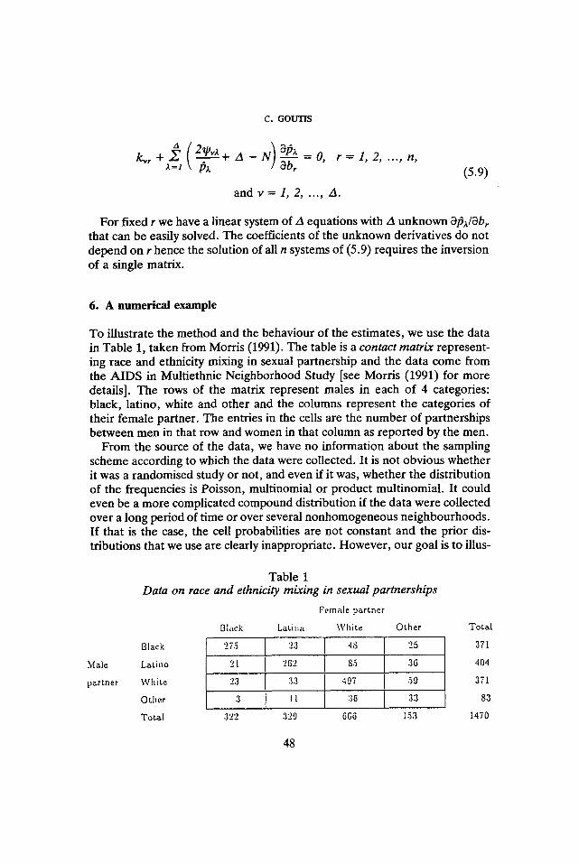
To illustrate the method and the behaviour of the estimates, we use the data in Table 1, taken from Morris (1991). The table is a contact matrix represent- ing race and ethnicity mixing in sexual partnership and the data come from the AIDS in Multiethnic Neighborhood Study [see Morris (1991) for more details]. The rows of the matrix represent males in each of 4 categories: black, latino, white and other and the columns represent the categories of their female partner. The entries in the cells are the number of partnerships between men in that row and women in that column as repor ted by the men.

From the source of the data, we have no information about the sampling scheme according to which the data were collected. It is not obvious whether it was a randomised study or not, and even if it was, whether the distribution of the frequencies is Poisson, multinomial or product multinomial. It could even be a more complicated compound distribution if the data were collected over a long period of time or over several nonhomogeneous neighbourhoods. If that is the case, the cell probabilities are not constant and the prior distributions that we use are clearly inappropriate. However , our goal is to illus-

Male

partner

Table 1 Data on race and ethnicity mix ing in sexual partnerships

Female partner

Black Latiua White Other

Black

Ladno

White

Other

ToLal

275 23 48

21 '26'2

23 33

3 II

322 329

85

25

36

497 59

36 33

666 153

Total

371

404

371

83

1470

48


trate the use of the priors rather than to provide a good model for the data, so for simplicity we will assume a multinomial likelihood. We should note that if the (row or column) margins are fixed by the sampling scheme the prior should be modified accordingly, as indicated in Section 3.

For such an example obviously we would not believe in independence of rows and columns. Given the separation of ethnic and racial groups in the society, we would expect that there will be a preferred mixing, favouring ingroup partnership. Hence one should treat the entries in the diagonal in a different way from the off diagonal entries. The counts on the diagonal would be expected to be large and probably different, since the proportion of races in the population are unequal. For the off diagonal elements, we suppose that we believe a priori that, once an individual is not related with somebody in their own group, there is no preferential t reatment of any other group. (Of course one may doubt it, in which case the prior that follows should be modified accordingly).

If we believed in complete independence, as shown in Section 2, a prior expressing it would be such that the subcomposition of the probabilities of each row would have similar parameters, and they could be derived by using a preliminary sample having a A 4 ( ~ R) distribution. However now, since we believe in preferred mixing we cannot use the same vector a for all rows. Recalling that a represents means of the log-counts, we can use as first parameters vectors of the form a + ~ is a vector having elements equal to zero, except the ith that is positive. Such a vector of means expresses the belief that a preliminary sample would be the same (apart from a multiplicative constant) for all rows for the off diagonal elements, but on the diagonal we expect a larger number. In the numerical results given later, we used empirical Bayes methdos, hence we did not specify a and rni. Of course specific values would yield the usual Bayes estimates.

We also prefer to have unequal variance-covariance matrices Ri. The reason is that the group ~Other~ is less well defined than the rest of the racial groups so we feel that 114 should be larger (in the eigenvalues sense) than Ri, i = 1, 2, 3, indicating more uncertainty for the counts in the fourth row. In the numerical results we used Rz = R2 = R3 = cR4 with c = 2, 10 and R1 = o21 with tr = 1, 0.1. Setting, at firs instance, tr = 1 can be interpreted as taking a coefficient of variation for each count equal to 1.311 and a = 0.1 translates to a coefficient of variation equal to 0.1, indicating a stronger belief in the above form of probabilities. We also tried a variance covariance matrix of the form R1 = o2((1 - Q)I + 0J) where J is a matrix of ones, with 0 = 0.5 indicating a weak positive correlation between counts of adjacent cells.

Assuming rather unrealistically but for mathematical simplicity that women and men behave the same way, we would expect the column pre-

49

C. GOUTIS

liminary samples to be similar to the row samples. Hence in column i the counts would have a A4(a + ~ , Ri) distribution, with ~ ~ and Ri as above. It is of course possible to specify or estimate different parameters.

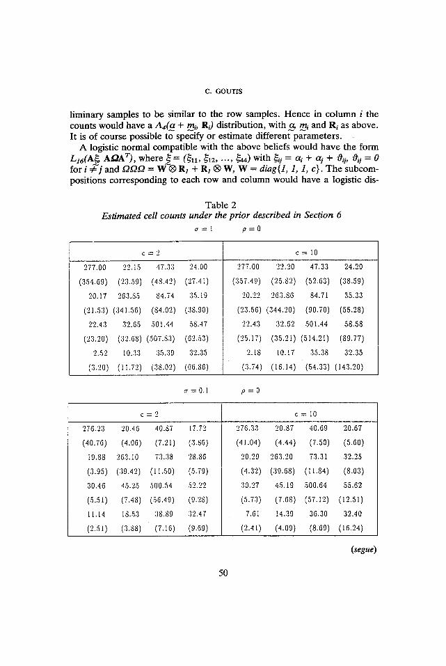
A logistic normal compatible with the above beliefs would have the form L16(A ~ AaA T), where ~ = (~u, ~12) ..., ~t4) w i t h ~ii = ai + a i 4- Oi], vqii = 0 for i :/7] and K2K2f2 = W~| R1 + R1 | W, W = diag{1, 1, 1, c}. The subcompositions corresponding to each row and column would have a logistic dis-

Table 2 Estimated cell counts under the prior described in Section 6

c r = l p = O

c='2 c = l O

277.00 22.15 47.33 24.00

(354.69) (23.59) (48.42)(27.41)

20.17 263.85 84.74 35.19

(21.53) (341.56) (84.02) (38.90)

22.43 32.65 501.44 58.47

(23.20) (32.68)(507.83) (62.53)

2.52 10.33 35.39 32.35

(3.20) (11.72) (38.02)

277.00 22.20 47.33 24.20

(357.49) (25.82) (52.63) (38.59)

20.22 263.86 84.71 35.33

(23.56) (344.20) (90.70) (55.28)

22.43 :}2.02 501.44 58.58

(25.17) (35.21) (514,21) (89.77)

2.18 10.17 35.38 32.35

(16.14) (54.33) (143.20) (66.86) (:}.74)

~=0.1 p = O

c = 2 c = 1 0

276.23 20.46 40.87 17.72

(40.76) (4.06) (7.21) (3.86)

19.88 263.i0 73.38 28.86

(3.95) (39.42) (11.50) (5.79)

30.46 45.25 500.54 52.22

(5.51) (7.48) (56.49) (9.28)

11.14 18.53 38.89 32.47

(2.51) (3.88) (7.16) (9.69)

276.3:} 20.87 40.69 20.67

(41.04) (4.44) (7.50) (5.60)

20.29 263.20 73.31 32.25

(4.32) (39.68) (11.84) (8.03)

30.27 45.19 500.64 55.62

(5.73) (7.68) (57.12) (12.51)

7.61 14.39 36.30 32.40

(2.41) (4.09) (8:69) (16.24)

50

(segue)

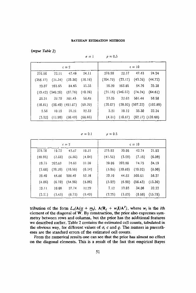
(segue Table 2)


~ = 1 p=0 .5

c = 2 c = 10

276.96 22.11 47.48 24.11

(358.17) (2i.:34) (:39.:38) (28.18)

20.07 26:3.85 84.85 35.:35

(19.42) (340.26) (67.76) (40.26)

22.:31 :32.70 501.45 58.48

(18.81) (26.49) (491.67) (60.29)

2.58 10.19 35.21 32.32

(3.32) (11.90) (36.49) (66.03)

276.09 22.17 47.43 24.24

(364.79) (23.17) (43.26) (44.72)

20.20 263.85 $4.76 35.38

(21.16) (346.,57) (74.24) (64.61)

')') :15 32.63 501.44 58.58

(20.67) (28.92)(507.32) (102.99)

2.21 10.12 35.30 32.34

(4.31) (18.67) (62.17)(139.60)

o" = 0.1 p = 0 . 5

c= '2 c = 10

275.76 19.72 42.87 19.31

(40.95) (3.68) (6.86) (4.04)

19.75 262.83 74.63 :11.36

(:3.68) (:39.20) (10.56) (6.14)

29.40 44.88 500.49 52.18

(4.86) (6.70) (54.96) (8.96)

10.11 16.66 3 7 . 7 4 32.29

(2.21) (3.43) (6.72) (9.49)

275.93 20,08 42,74 21.93

(41..58) (3.99) (7.15) (6.09)

20.06 262.98 74.75 34.19

(3.98) (39.80) (10.92) (8.90)

29,10 44,82 500.61 56.37

(5.02) (6.90) (56.43) (13.36)

7.12 13.03 34.06 32.22

(2.25) (:3.83) (8.58) (15.79)

t r ibut ion o f the fo rm L4(A(ff. + mi)., AOR1 + wiI)AT), where wi is the ith e lement o f the diagonal of W. By construct ion, the pr ior also expresses sym- me t ry be tween rows and columns, but the pr ior has the addit ional features we descr ibed earlier. Table 2 contains the es t imated cell counts , tabula ted in the obvious way, for different values o f o, c and Q. The numers in paren th- eses are the s tandard errors o f the es t imated cell counts.

F r o m the numerical results one can see that the pr ior has a lmost no effect on the diagonal elements. This is a result o f the fact that empirical Bayes

51

C. GOUTIS

procedures allow the estimation of Oii and each Oil corresponds to one cell, hence, in some sense, the prior will agree with the data for these cells. However the change in the off diagonal entries is at times substantial. A s explained earlier we obtain estimates different form the data by decreasing the prior uncertainty o, when the estimates are closer to the restricted maximum likelihood estimates. Decreasing tr has also a dramatic effect on the posterior variance of estimates. The constant c influences essentially only the last row and column, since different values are meant to indicate different degrees of prior uncertainty in the conditional probabilities for the last row and column. Perhaps surprisingly, different values of p give almost identical results. Other values that we tried (not shown in the Table), had no large effect either, unless IQ] ~ 1 indicating a perhaps unrealistically strong dependence between cells in the same row or column. A possible explanation is that it is not so much the form of the prior variance covariance matrix that is important as it is the magnitude of the matrix and the submatrices corespond- ing to subcompositions of interest.

Acknowledgment

I would like to thank J. Burridge and C. E. McCulloch for useful discussions and two referees whose comments improved an earlier version of the paper.

R E F E R E N C E S

AITCHISON, J. (1982), The statistical analysis of compositional data (with discussion), J. R. Statist. Soc. Ser. B, 44, 139-177.

AITcmsor% J. (1985a), Practical Bayesian problems in simplex sample spaces, in Pro- ceedings of the second international meeting on Bayesian statistics (J. M. Bernardo, M. H. DeGroot, D. V. Lindley and A. F. M. Smith, eds.), pp. 15-32. Amsterdam: North Holland.

ArrcHISON, J. (1985b), A general class of distributions on the simplex, J. R. Statist. Soc. Ser. B, 47, 136-146.

ArrcHISON, J. (1986), The statistical analysis of compositional data, London: Chapman & Hall.

AITCHISON, J. and SHEN, S. M. (1980), Logistic-normal distributions: some properties and uses, Biometrika, 67, 261-272.

ALBERT, J. H. (1985), Simultaneous estimation of Poisson means under exchangeable and independence models, J. Statist. Comput. Simulat., 23, 1-14.

ALBERT, J. H. (1988), Computational methods using a Bayesian hierarchical generalized linear model, J. Amer. Statist. Assoc., 83, 1037-1044.

52


ALBERT, J. H. and GUPTA, A. K. (1982), Mixture of Dirichlet distributions and estimation in contingency tables, Ann. Statist., 10, 1261-1268.

ALBERT, J. H. and GUrrA, A. K. (1983a), Bayesian estimation methods for 2 x 2 contingency tables using mixtures of Dirichlet distributions, J. Amer. Statist. Assoc., 78,708-717.

ALBERT, J. H. and GuZrA, A. K. (1983b), Estimation in contingency tables using prior information, J. R. Statist. Soc. Ser.B, 45, 60-69.

ALa'HAM, P. M. E. (1969), Exact Bayesian analysis of 2 x 2 contingency table and Fisher's "exact" significance test, J. R. Statist. Soc. Ser. B, 31,261-269.

BISHOP, Y. M. M., FIENBERG, S. E. and HOLLAND, P. W. (1975), Discrete Multivariate Analysis: Theory and Practice, Cambridge, Mass: The MIT press. '.

BLOCH, D. A. and WATSON, G. S. (1967), A Bayesian study of the multinomial distribution, Ann. Math. Statist, 38, 1423-1435.

CROOK, J. R. and GOOD, I. J. (1980), On the application of symmetric Dirichlet distributions and their mixtures to contingency tables, part II, Ann. Statist., 8, 1198- 1218.

DAWlD, A. P. (1982), Discussion on <<The statistical analysis of compositional data>> by J. Aitchison, J. R. Statist. Soc. Ser. B, 44, 139-177.

DEMPSTER, A. P., LAIRD, N. M. and RUBIN, D. B. (1977), Maximum likelihood from incomplete data via the EM algorithm (with discussion), J. R. Statist. Soc. Ser. B, 39, 1-38.

GOOD, I. J. (1976), On the application of symmetric Dirichlet distributions and their mixtures to contingency tables, Ann. Statist. 4, 1159-1189.

GOUTIS, C. (1993), Recovering extra-binomial variation, J. Statist. Comput. Simulat., 45, 233-242.

GUPTA, A. K., SALEH, A. K. MD. E. and SEN, P. K. (1989), Improved estimation in a contingency table: independence structure, J. Amer. Statist. Assoc., 84,525-532.

KASS, R. E. and STEFFEY, D. (1989), Approximate Bayesian inference in conditionally independent hierarchical models (parametric empirical Bayes models), J. Amer. Statist. Assoc., 84, 717-726.

LAIRD, N. M. (1978), Empirical Bayes estimation for two-way contingency tables, Biometrika, 65, 581-590.

LEONARD, T. (1972), Bayesian methods for binomial data, Biometrika, 59, 581-589. LEONARD, T. (1973), A Bayesian method for histograms, Biometrika, 60, 297-308. LEONARD, Z. (1975), Bayesian estimation methods for two-way contingency tables, J.

R. Statist. Soc. Ser. B, 37, 23-37. LEONARD, T. and NovicK, M. R. (1986), Bayesian full rank marginalization for two-

way contingency tables, J. Educ. Statist., 11, 33-56.

LINDLEY, D. V. (1964), The Bayesian analysis of contingency tables, Ann. Math. Statist., 35, 1622-1643.

53

C. GOUTIS

LINDLEY, D. V. and SmTH, A. F. M. (1972), Bayes estimates for the linear model (with discussion), J. R. Statist. Soc. Set. B, 34, 1-41.

McGuLLAGH, P. and NELDER, J. A. (1989), Generalized Linear Model, 2 nd edition, London: Chapman & Hall.

Mol~aS, C. (1983), Parametric empirical Bayes inference: theory and practice, J. Amer. Statist. Assoc., 78, 47-65.

MORRIS, M. (1991), A log-linear modeling framework for selective mixing, Math. Biosci., 107, 349-377,

NAZARET, W. A. (1987), Bayesian log liner estimates for three-way contingency tables, Biometrika, 74, 401-410.

PmGORSCH, W. W. and CASELLA, G. (1990), Empirical Bayes estimation for generalized linear models, Biometrics Unit Technical Report, BU-1067-M, Cornell Uni- versity.

PROTrER, M. H. and MORREY, C. B. (1977), A First Course in Real Analysis, New York: Springer-Verlag.

STEFFEY, D. and KASS, R. E. (1991), Discussion on <<That BLUP is a good thing: the estimation of random effects>} by G.K. Robinson, Statist. Sci., 6, 15-51.

TIEmqEY, L. and KADANE, J. B. (1986), Accurate approximations for posterior mo- ments and marginal densities, J. Amer. Statist. Assoc., 81, 82-86.

TIE~EV, L., KASS, R. E. and KADAN~., J. B. (1989), Fully Laplace approximation to expectations and variances of nonpositive functions, J. Amer. Statist. Assoc., 84, 710-716.

54

Documents

Bayesian estimation methods for contingency tables