Bayesian decision theoretic two-stage design in phase II

Research Article

Received 5 January 2011, Accepted 8 December 2011 Published online 23 February 2012 in Wiley Online Library

(wileyonlinelibrary.com) DOI: 10.1002/sim.4511

Bayesian decision theoretic two-stagedesign in phase II clinical trials withsurvival endpointLili Zhao,a*† Jeremy M. G. Taylorb and Scott M. Schuetzec

In this paper, we consider two-stage designs with failure-time endpoints in single-arm phase II trials. We pro-pose designs in which stopping rules are constructed by comparing the Bayes risk of stopping at stage I with theexpected Bayes risk of continuing to stage II using both the observed data in stage I and the predicted survivaldata in stage II. Terminal decision rules are constructed by comparing the posterior expected loss of a rejectiondecision versus an acceptance decision. Simple threshold loss functions are applied to time-to-event data modeledeither parametrically or nonparametrically, and the cost parameters in the loss structure are calibrated to obtaindesired type I error and power. We ran simulation studies to evaluate design properties including types I andII errors, probability of early stopping, expected sample size, and expected trial duration and compared themwith the Simon two-stage designs and a design, which is an extension of the Simon’s designs with time-to-eventendpoints. An example based on a recently conducted phase II sarcoma trial illustrates the method. Copyright© 2012 John Wiley & Sons, Ltd.

Keywords: Bayesian; decision theory; time to event; phase II clinical trial; two-stage design

1. Introduction

In phase II cancer clinical trials, the standard approach consists of a single-arm design where a singlebinary endpoint is compared with a specified target value. The sample sizes are typically small, maybe30�70 patients. Improvements to the study could be made by increasing the sample size, using random-ization and using an endpoint that is more informative than a binary one. Limitations on the availablenumber of patients frequently limits power for a randomized study. Our focus in this paper will be onenhancing the trials using nonbinary endpoints. We will consider designs with failure-time endpoints,measuring time until some event, such as a device-related complication, disease progression, relapse,or death. Progression-free survival (PFS) is increasingly used as an endpoint for cancer clinical trials,and a recent review suggests that PFS is being utilized more commonly and may predict for greater suc-cess in the phase III setting [1]. Using PFS as an endpoint in single-arm studies does raise some issuesconcerning the possibility of bias in the comparison with the historical control group [2–4]. Althoughthere is always the possibility of differences in the populations and in methods for assessing the endpointbetween the trial and the control group, when using PFS, a consistent surveillance strategy for assessingprogression is also needed.

A single-arm phase II trial is typically designed to accrue patients in two stages [5–7], with the Simondesign being very popular. It will stop at stage I if a preset level of futility has been demonstrated, therebyreducing the number of patients exposed to an ineffective therapy. Similar to classical phase II studies, astudy based on a time-to-event endpoint (such as median PFS or PFS rate at a specific clinical landmarkpoint, t0) will be deemed a success if there is sufficient statistical evidence to conclude that the endpoint

aBiostatistics Unit, University of Michigan Comprehensive Cancer Center, Ann Arbor, MI 48109, U.S.A.bDepartment of Biostatistics, University of Michigan, Ann Arbor, MI 48109, U.S.A.cDepartment of Internal Medicine, University of Michigan, Ann Arbor, MI 48109, U.S.A.*Correspondence to: Lili Zhao, Biostatistics Unit, University of Michigan Comprehensive Cancer Center, Ann Arbor,MI 48109, U.S.A.

†E-mail: [email protected]

1804

Copyright © 2012 John Wiley & Sons, Ltd. Statist. Med. 2012, 31 1804–1820

L. ZHAO, J. M. G. TAYLOR AND S. M. SCHUETZE

exceeds, at a clinically relevant level, that of a relevant historical control. Many statistical designs arebased on the probability that the patient survives to specific time t0 without suffering the event. Themost severe problem created by this approach is that a patient has to be followed-up for t0 time to ensurethat event has not occurred, and waiting until all patients in stage I complete the follow-up of t0 maycause long recruitment suspension especially when t0 is large. The impact of study suspension on accrualmomentum and timeliness of the studies completion is often negative. A number of authors have formu-lated underlying statistical models and interim decision rules directly in terms of time-to-event variablesto overcome this problem. Herndon [8] proposed a frequentist ad hoc approach to conducting two-stagephase II studies to avoid study suspension. Case and Morgan [9] proposed frequentist two-stage phaseII designs using the estimator developed by Lin et al. [10] to minimize the expected sample size orexpected total study length (ETSL) under H0. Huang et al. [11] modified their approach to protect type Ierror rate and improve robustness of the design. These designs [9, 11] are essentially an extension of theSimon designs with failure time endpoints using nonparametric statistics.

Researchers developed several Bayesian approaches to continuously monitor survival endpoints.Follman and Albert [12] used a Dirichlet process prior for the probabilities of the event on a large set ofpotential discretized event times. They compute an approximate posterior distribution that is a mixtureof Dirichlet processes by using a data augmentation algorithm. Rosner [13] took a similar approach butused Gibbs sampling to generate posteriors. Cheung and Thall [14] constructed futility monitoring ruleson the basis of an approximate posterior through a weighted average of beta distributions for one ormore event times in phase II trials. These approaches incorporate the censored data into the posteriorestimation in a nonparametric fashion. Thall et al. [15] developed model-based approaches to monitortime-to-event endpoints, assuming exponentially distributed failure times with an inverse gamma prioron the mean. They also examined the robustness of the method by assuming that the survival data followsa generalized gamma distribution. In the aforementioned Bayesian designs (e.g., [14, 15]), decisions aremade using the posterior distribution of the clinically relevant survival endpoints, and the futility mon-itoring rule is typically based on P.pE > pS C ıjdata/ < pL . Thus, the trial is stopped early if theposterior probability that pE (such as median survival or survival rate at a specific time point of theexperimental treatment) exceeds a clinical meaningful threshold (ı) over the traditional treatment pSby less than a prespecified cutoff, pL. The pL can be calibrated by simulations to obtain good trialproperties such as probability of early termination, type I error, and power [16].

The property of Bayesian procedures to accumulate evidence based on updated data is very attractivein clinical trial designs. However, at the end of stage I, most investigators are interested in knowingwhat is the probability that the study would yield a significant result in favor of the new treatment ifthe study were to be continued to stage II, given what has been observed to date. Lachin [17] reviewedmany frequentist approaches that construct stopping rules on the basis of an assessment of this ideausing (predictive) conditional power. Pepe and Anderson [18] presented expressions for the types I andII error probabilities for use with time-to-event endpoints assuming current trends continue for survivaldata. Berry [19] is also a strong advocate for the use of predictive probabilities in making decisions.However, the aforementioned approaches (frequentist or Bayesian) use only the predictive distributionto make interim decisions. In this paper, we will weight the evidence for stopping or continuing on thebasis of posterior and predictive distributions. Once the trial is stopped, the posterior distribution is usedfor making terminal decisions.

In the literature, researchers have developed decision-based Bayesian methods for binary endpoints[20–24]. Zhao and Woodworth [25] proposed a decision-based Bayesian approach for continually mon-itoring survival endpoints in single-arm phase II trials with medical devices, but the time-to-event datawas assumed to be exponentially distributed.

In practice, the decision theoretic clinical trial designs remain relatively uncommon. The main rea-sons for this lack of application are fundamental concerns with the decision theoretic setup and practicaldifficulty of specifying a good loss function [26]. In decision-theoretic approaches, costs need to bespecified, and in most situations, it is very hard to relate the costs to tangible quantities. Our strategy tomake this approach feasible is to treat the cost parameters, defined in a simple loss structure, as tuningparameters, which are calibrated to achieve desired operating characteristics such as type I error andpower. This approach alleviate concerns about difficulties in specifying the loss function, and as we willshow, the properties of the decision theoretic designs appear to be very attractive.

Section 2 presents the general framework and methodology. Section 3 contains simulation studies toevaluate the properties of the proposed methods and compares the results to two frequentist designs.Section 4 contains results from a phase II sarcoma trial. Section 5 is the concluding discussion.


1805


2. Method

The primary endpoint is a time-to-event outcome at some clinically meaningful landmark point t0; suchas 6 months or 1 year from the start of the treatment. Let S.t0/ be the survival rate at t0. Similar to mostother designs with a binary endpoint of tumor response, decisions are made based on two hypotheses H0:S.t0/ 6 p1 that the true survival rate at t0 is less than some uninteresting level p1 and H1: S.t0/ > p2that the survival rate is at least some desirable target level p2.

With right-censored data, the likelihood for n subjects is

L.‚jD/D

nYiD1

ff .ti /gıi fS.ti /g

1�ıi

and

S.t0/D e�H.t0/; where H.t0/D

Z t0

0

h.u/ du;

where‚ are the parameters that determine the distribution f .t/ and D is the observed data, which includesurvival times, t D .t1; t2; : : : ; tn/ and corresponding indicators of censoring, ı D .ı1; ı2; : : : ; ın/.

In this paper, we have chosen a very simple loss function as specified in Table I. There are two pos-sible wrong decisions: (1) false rejection (type I error) and (2) false acceptance (type II error). c2 is thepenalty you are willing to pay for a false rejection decision over a false acceptance decision. In deci-sion theory, c2 could be a function of the sample size or could differ from stage I to stage II. In thispaper, not to overcomplicate things, we consider c2 as fixed and treat c2 as a tuning parameter to controltype I error and power. A rejection decision will be made if the posterior expected loss of making arejection decision (e.g., c2P.S.t0/ <D p1jD/) is less than that of making an acceptance decision (e.g.,P.S.t0/ >D p2jD/), and an acceptance decision will be made otherwise. The higher the c2, the lesslikely we are going to reject H0 to avoid the high penalty of a false rejection decision. But before wedecide to stop and make a terminal decision (reject or accept H0), we should compare the risk of stop-ping at stage I to the ‘expected’ risk if the trial will be continued to stage II. The (posterior) Bayes risk ofimmediate stopping at stage I, denoted by �0.�1/; is defined as the minimum of the (posterior) expectedlosses under two decisions,

�0.�1/DminfP.S.t0/> p2jD1/; c2P.S.t0/6 p1jD1/g

whereD1 are the observed data up to stage I; �1 is the posterior distribution of S.t0/ given the observeddata up to stage I, denoted by f .S.t0/jD1/.

The expected (posterior) Bayes risk of continuing to stage II, denoted by �c.�1/, is defined as,

�c.�1/D ED2jD1 Œ�0.�

2/�C c3 (1)

D ED2jD1 ŒminfP.S.t0/> p2jD2/; c2P.S.t0/6 p1jD2/g�C c3 (2)

Table I. Threshold loss structure.

True status of the treatmentNoninferior

Inferior Neither Superior.S.t0/6 p1/ .p1 < S.t0/ < p2/ .S.t0/> p2/

Accept H0 0 0 1

DecisionReject H0 c2 0 0

1806



where �2 is the posterior distribution of S.t0/ given the observed data up to stage II, denoted byf .S.t0/jD2/. c3 is the cost of running the trial to the final stage, which could be a function of thesample size or study length in stage II. In this paper, c3 is also fixed to control the probability of stoppingat the end of stage I. The higher the c3, the more likely the trial will be halted at stage I to avoid the highcost of continuing the trial. ED2jD1 Œ�0.�

2/� defined in (1) can be approximated by

ED2jD1 Œ�0.�2/��

1

B

BXlD1

Œ�0.�2;l/� when B is large: (3)

where �2;l is f .S.t0/jD2;l/ andD2;l (l D 1; 2; : : : ; B) are the random samples of potential datasetsD2generated given D1.

In brief, the decision rule is as follows:

� At the end of stage I

- if �0.�1/6 �c.�1/, then stop and* Reject H0 if P.S.t0/>p2jD1/

P.S.t0/<p1jD1/> c2

* Accept otherwise- else if �0.�1/ > �c.�1/, then continue to stage II

� At the end of stage II, stop and

- Reject H0 if P.S.t0/>p2jD2/P.S.t0/<p1jD2/

> c2- Accept otherwise

The aforementioned decision rules are attractive for two reasons. First, the terminal decision rule isconstructed using the ratio of two posterior probabilities under two hypotheses (e.g., similar to posteriorodds). Second, the decision to ‘stop’ or ‘continue’ is the result of weighting the evidence between theobserved data and the data that will be observed if the trial would continue.

Once the posterior distribution of‚ is known, the distribution of S.t0/; as a function of‚, can be com-puted using Monte Carlo methods. Therefore, it is easy to calculate the posterior probabilities under thetwo hypotheses. It is, however, much harder to calculate the Bayes risk of continuation, which involvesthe posterior predictive distribution of D2 given D1 in the presence of censoring. In the following sec-tion, we derive algorithms to estimateED2jD1 Œ�0.�

2/� for exponential failure time distributions, Weibulldistributions, and time-to-event data that do not follow any parametric distribution.

2.1. Method assuming exponential distribution

Assume the time-to-event data follows an exponential distribution, f .t/ D �e��t for t > 0; and theprimary endpoint S.t0/ is defined as S.t0/D e��t0 .

The likelihood function for � at stage k is L.�jDk/ D �fke��e

k, where f k is the total number

of failures and ek is the total exposure time up to stage k (k D 1; 2). These are sufficient statistics toestimate �. D then can be simplified to D1 D .f 1; e1/ and D2 D .f 2; e2/: For mathematical conve-nience, we use the conjugate prior for � such that � � �.˛0; ˇ0/. Then, the posterior distribution iseasily determined to be a Gamma distribution, f .�jDk/� �.˛0C f k; ˇ0C ek/:

Given the data up to stage I (D1), we can simulate the patients’ survival data in stage II. The numberof patients in stage II (denoted by N2) has two parts: (1) the number of event-free patients that havenot reached the final study point at the end of stage I; and (2) the number of new patients recruited instage II. Because of the ‘lack of memory” property of the exponential distribution, those patients that areevent free at the end of stage I are conditionally exchangeable with patients who are recruited in stageII, and their survival times in stage II will also be distributed as an exponential distribution with rate� � �.˛0 C f

1; ˇ0 C e1/. Zhao and Woodworth [25] defined the algorithm to obtain samples of D2

given D1.

2.2. Method assuming Weibull distribution

The Weibull distribution, denoted by W.˛; �/, is f .t/D ˛�t˛�1e��t˛

for t > 0; ˛ > 0, and � > 0. Let‚D .˛; �/ and the primary endpoint is S.t0/D e��t

˛0 :

In this case, Dk D .tk; ık/; k D 1; 2. tk includes all survival times for patients enrolled up to stagek, and ık are the corresponding censoring indicators. Unlike the exponential distribution, there are no


1807


simple sufficient statistics and no simple posterior distributions for ˛ and � . MCMC methods will beused to estimate these two parameters.

This Weibull model can be expressed as a log-linear model as log tiD� C i [27], where � D� log.�/=˛ and D 1=˛: The density of the log time, yi D log ti , is given by

f .yi /D1

exp.í � e

í /; where í Dyi ��

If we assign � a uniform prior and for the usual noninformative prior proportional to 1= , then theposterior density is given by

f .�; jDk//1

L.�; jDk/; k D 1; 2 (4)

Metropolis–Hasting algorithms can easily be applied to estimate � and .Given the data up to stage I (D1 D .t1; ı1/), survival times for patients enrolled in stage II will be

generated from a Weibull distribution with the updated‚ from stage I. For any patient i that is censoredat the end of stage I and has not reached the final study point, the probability that the patient will surviveadditional time xi is expressed as

S.xi /D P.t > t1i C xi jt > t

1i /D e

��.t1i Cxi/

˛�t1i

˛�

(5)

To simulate this additional time, we simulate S.xi;l/ from U.0; 1/, and solving for x gives

xi;l D

�� log.S.xi;l//

�lC t1i

˛l

� 1˛l

� t1i ;

where ˛l and �l are from the l th MCMC iteration. Then, xi;l ; l D 1; : : : ; B are random samples fromthe posterior predictive distribution of the remaining survival time of patient i in stage II.

Let t2i;lD minft1i C xi;l ;Mig, ı2i;l D 1 if t2

i;l<Mi and ı2

i;lD 0 otherwise, where Mi is the maximum

follow-up for patient i defined from the enrollment to the final study time point. We repeat this processfor all patients (i D 1; : : : ; N2) in stage II, and together with the observed survival data of patients thathad event, we obtain D2;l . Then, D2;1; : : : ;D2;B form a random sample from the posterior predictivedistribution of f .D2jD1/:

Similar methods can be developed assuming Gamma or log-normal distributions.

2.3. Grouped-data method

In practice, interval-censored survival data is common in medical settings where the patient’s diseasestatus is evaluated periodically by tests such as magnetic resonance imaging or computed axial tomog-raphy scan. The actual time of any patients disease progression is not available, rather, it is only knownwhether progression occurred during each time interval between successive examinations. To accountfor this type of interval censoring, we propose a nonparametric method in this section, which handlesthe interval-censored data for various time-to-event data distributions.

Given the data up to stage I (D1), we construct a finite partition of the time axis, 0 < s1 < s2 <

� � � < sJ ; with sJ D t0. Thus, we have the J disjoint intervals .0; s1�; .s1; s2�; : : : ; .sJ�1; sJ �; andIj D .sj�1; sj �. The value of sj .j D 1; : : : ; J /, in the interval-censored case, should be determined bythe intended gap between two consecutive scheduled appointments. For example, the scheduled appoint-ment is every 2 months for the first half year, then the intervals can be set up as s1 D 2; s2 D 4; s3 D 6;and J D 3. For studies where the evaluation is more frequent, the value of J would be much larger.

The observed data D is assumed to be available as grouped within these intervals such that Dk D.Rk

j ;Dkj W j D 1; 2; : : : ; J /; where Rkj is the risk set and Dkj is the failure set of the j th interval Ij up

to stage k. Let hj denote the increment in the cumulative baseline hazard in the j th interval, that is,

hj DH0.sj /�H0.sj�1/; j D 1; 2; : : : ; J (6)

1808



and

S.t0/D exp

0@�

JXjD1

hj

1A

The grouped data likelihood is

L.hjDk//JYjD1

Gkj ; hD .h1; h2; : : : ; hJ /

and

Gkj D expn�hkj

�rkj � d

kj

�o n1� exp

��hkj

�odkj

(7)

where rkj and dkj are the number of subjects in the sets Rki and Dkj up to stage k, respectively.

The Gamma process is used as a prior for the cumulative baseline hazard function H0.t/ [28]such that

H0 � GP.�0H�; �0/; (8)

whereH�.t/ is an increasing function withH�.0/D 0: H� is assumed to be a Weibull distribution withhyperparameter �0 and 0; such that H�.t/ D �0t

�0 : �0 is a positive scalar quantifying the degree ofprior confidence in H�.t/: If 0 D 1, this simplifies as an exponential distribution with rate �0.

The Gamma process prior in (8) implies that hj ’s are independent and

hj � �.�0.H�.sj /�H

�.sj�1//; �0/: (9)

With the likelihood and priors set up as that previously discussed, we can write the posteriordistribution of h as specified in [29]

f .hjDk//JYjD1

Gkj h�0.H

�.sj /�H�.sj�1//�1

j e�0hj (10)

We can carry out the following Gibbs sampling scheme sampling hj from

�.hj jh�j ;Dk//Gkj h

�0.H�.sj /�H

�.sj�1//�1

j e�0hj (11)

where h�j denote the h vector without j th component. Plugging in the form for Gkj from Equation (7),we have

�.hj jh�j ;Dk// h�0.H

�.sj /�H�.sj�1//�1

j .1� e�hj /dkj e�.�0Cr

kj�dkj/hj : (12)

Survival times are approximated by piecewise constant hazard survival model. Thus, the memorylessproperty of the exponential distribution holds in each interval Ij ; j D 1; 2; : : : ; J . Given data observedup to stage I (D1), survival times for patients in stage II (i D 1; : : : ; N2) will be generated on the basisof the updated h1; : : : ; hJ . For any patient i that is censored in interval Ij at the end of stage I andhas not reached the final study point, the remaining survival time, xi;j;l ; will first be generated from

an exponential distribution with rate hjsj�sj�1

, then moving from left to right along the time line untilthe event occurs or the final study time point is reached, which will result in generated survival times,xi;j;l ; xi;jC1;l ; : : : in intervals Ij ; IjC1; : : : ; respectively. Let ti;j;l D minfxi;j;l ; .minfsj ;Mig � t

1i /gI

if ti;j;l D sj � t1i (no event occurred in Ij and the final study point has not been reached), we will

move to IjC1. If no event occurred in IjC1 and Mi > sjC1; then ti;jC1;l D sjC1 � sj . Finally,


1809


t2i;lD t1i C ti;j;l C ti;jC1;l C : : : : For patients enrolled in stage II, this process starts at I1. We repeat

this process for all patients (i D 1; : : : ; N2) in stage II to obtain a random sample from the posteriorpredictive distribution of f .D2jD1/.

We note that with the use of a large number of intervals, this grouped-data method can be viewedas a nonparametric method for general distributions that would be applicable even if the data were notinterval censored.

3. Simulation studies

In this section, we ran simulations to investigate properties of the proposed designs (Bayes designs)including type I error, power, probability of early stopping (PET), expected sample size, and ETSL underboth null and alternative hypotheses. In the simulation setup, we assumed the landmark time point, t0,to be 6 months; we took the interim analysis 1 day before the first patient of stage II was enrolled suchthat there is no trial suspension and defined the final study point as 6 months after the enrollment of thelast patient; the maximum follow-up per patient is 12 months; we sampled the patient arrival time froma Poisson distribution with a rate of 0.1 so that one patient arrives an average of every 10 days.

In Simon’s designs, we dichotomize the survival time into a binary variable I.t 6 t0). With suchdesigns, the trial will continue immediately to stage II once the number of successes reaches the thresh-old rather than waiting for all enrolled patients to complete the follow-up and stops immediately if thereis no hope that the threshold will be met. For example, consider the situation where three successes of10 is needed for the trial to continue to stage II. If only one success is observed for the first nine patientsthat had completed the follow-up, the trial should stop even though the last patient has not completed thefollow-up because we would observe at most two successes in this case. For the Simon designs, we willconsider both the MiniMax and the optimal designs. To be comparable with the Simon’s designs, whichonly allow early stopping for futility, the stopping rule in the Bayes design is modified as

�c > �0 andP.S.t0/ > p2jD1/

P.S.t0/ < p1jD1/6 c2:

This ‘Stop only for futility’ rule is used throughout the simulations unless specified otherwise.As well as comparing with the Simon designs, we will also make comparisons with the method

described in [11]. This method prevents trial suspension by using Nelson–Aalen estimates of the sur-vival calculated at different calendar times to account for the information available from those withpartial follow-up. We implemented this method using the R program OptimPhase2.

3.1. Effect of the cost parameters

In this simple loss structure, cost parameter c2 controls the trade-off between types I and II errors andcost parameter c3 controls the PET. In this section, we investigated the effect of c2 and c3 while fixing theother. We calculated total sample size (nD 47) and the sample size in stage I (n1 D 24) from the SimonMiniMax design by restricting type I error to be 0.05 and type II error to be 0:15 with the two decisionthresholds p1 D 0:1 and p2 D 0:25: We generated survival data from an exponential distribution withrate � logS.t0/

t0;where S.t0/ D 0:1 or 0:25: We used an uninformative Gamma prior distribution, with

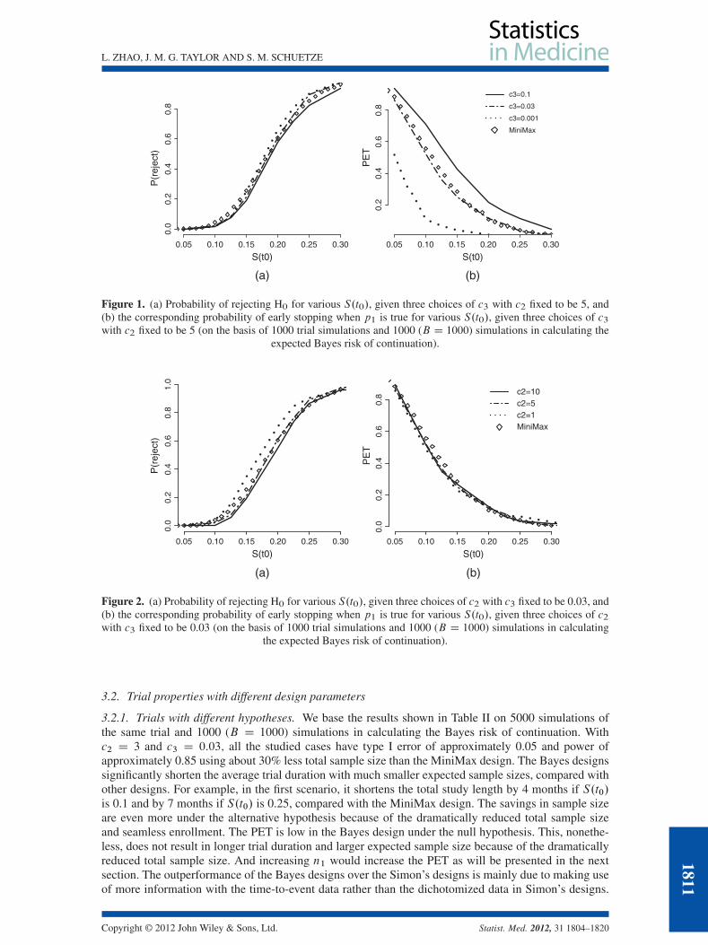
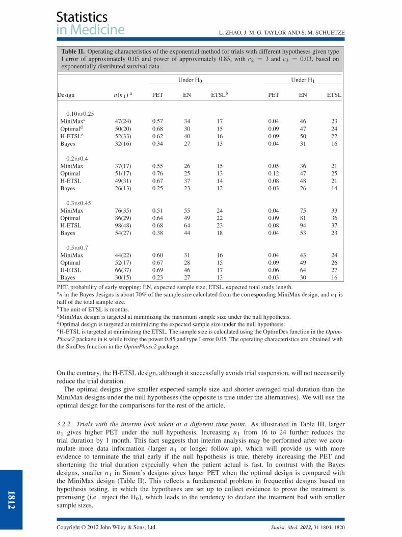
mean 0.0001 and rate 0.0001, for �.Figure 1 demonstrates the effect of c3 when c2 is fixed to be 5. The highest c3 (e.g., c3 D 0:1) gives

the highest PET across different S.t0), and c3 of 0.03 provides similar PET as the MiniMax design. InFigure 2, c3 is fixed to be 0.03. The highest c2 (e.g., c2 D 10) has the lowest probability of rejecting theH0; resulting in the lowest power at S.t0/ D 0:25 as well as the lowest type I error at S.t0/ D 0:1. Wefound that the choice of c2 D 3 and c3 D 0:03 gives type I error of 0.03 and power of 0.9. To obtainapproximately type I error of 0.05 and power of approximately 0.85, to match the MiniMax design, wereduced the sample size by 32% to nD 32 given c2 D 3 and c3 D 0:03. With this sample size, we investi-gated the operating characteristics of trials with different design parameters such as different hypotheses(p1 and p2), different patient accrual rates, different timing of the interim look, a stopping rule thatallows stopping for both efficacy and futility, and different prespecified values for types I and II errors.Without loss of generality, we used the exponential method for data that are exponentially distributed.

1810



0.05 0.10 0.15 0.20 0.25 0.30

0.0

0.2

0.4

0.6

0.8

S(t0)

P(r

ejec

t)

0.05 0.10 0.15 0.20 0.25 0.30

0.2

0.4

0.6

0.8

S(t0)

PE

T

c3=0.1

c3=0.03

c3=0.001

MiniMax

(b)(a)

Figure 1. (a) Probability of rejecting H0 for various S.t0/, given three choices of c3 with c2 fixed to be 5, and(b) the corresponding probability of early stopping when p1 is true for various S.t0/, given three choices of c3with c2 fixed to be 5 (on the basis of 1000 trial simulations and 1000 (B D 1000) simulations in calculating the

expected Bayes risk of continuation).

0.05 0.10 0.15 0.20 0.25 0.30

0.0

0.2

0.4

0.6

0.8

1.0

S(t0)

P(r

ejec

t)

0.05 0.10 0.15 0.20 0.25 0.30

0.0

0.2

0.4

0.6

0.8

S(t0)

PE

T

c2=10c2=5c2=1MiniMax

(b)(a)

Figure 2. (a) Probability of rejecting H0 for various S.t0/, given three choices of c2 with c3 fixed to be 0.03, and(b) the corresponding probability of early stopping when p1 is true for various S.t0/, given three choices of c2with c3 fixed to be 0.03 (on the basis of 1000 trial simulations and 1000 (B D 1000) simulations in calculating

the expected Bayes risk of continuation).

3.2. Trial properties with different design parameters

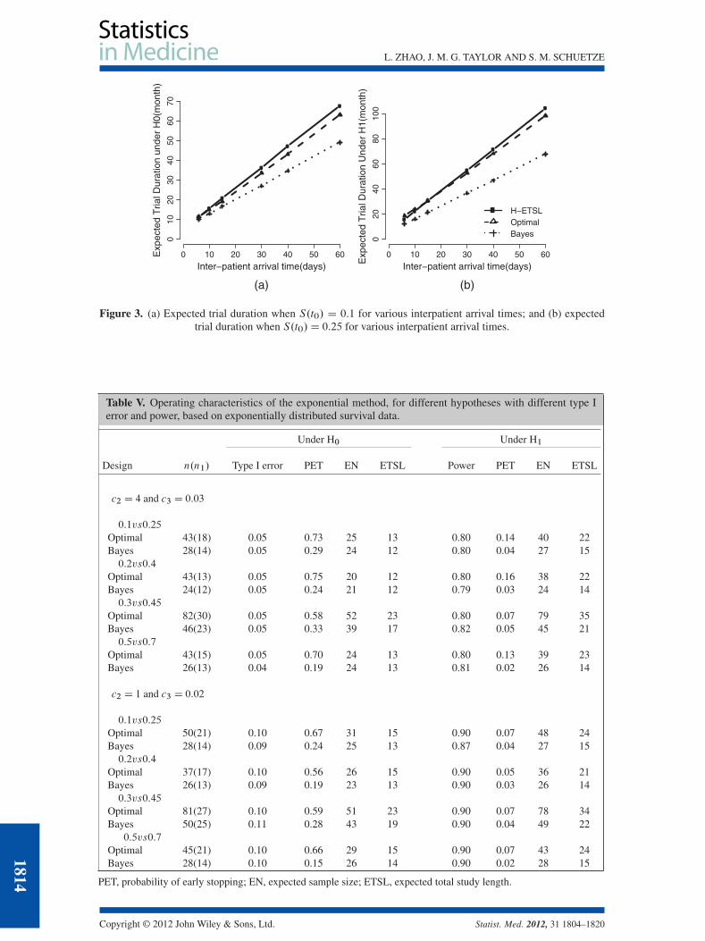
3.2.1. Trials with different hypotheses. We base the results shown in Table II on 5000 simulations ofthe same trial and 1000 (B D 1000) simulations in calculating the Bayes risk of continuation. Withc2 D 3 and c3 D 0:03; all the studied cases have type I error of approximately 0.05 and power ofapproximately 0.85 using about 30% less total sample size than the MiniMax design. The Bayes designssignificantly shorten the average trial duration with much smaller expected sample sizes, compared withother designs. For example, in the first scenario, it shortens the total study length by 4 months if S.t0/is 0.1 and by 7 months if S.t0/ is 0.25, compared with the MiniMax design. The savings in sample sizeare even more under the alternative hypothesis because of the dramatically reduced total sample sizeand seamless enrollment. The PET is low in the Bayes design under the null hypothesis. This, nonethe-less, does not result in longer trial duration and larger expected sample size because of the dramaticallyreduced total sample size. And increasing n1 would increase the PET as will be presented in the nextsection. The outperformance of the Bayes designs over the Simon’s designs is mainly due to making useof more information with the time-to-event data rather than the dichotomized data in Simon’s designs.


1811


Table II. Operating characteristics of the exponential method for trials with different hypotheses given typeI error of approximately 0.05 and power of approximately 0.85, with c2 D 3 and c3 D 0:03, based onexponentially distributed survival data.

Under H0 Under H1

Design n.n1/a PET EN ETSLb PET EN ETSL

0:10vs0:25

MiniMaxc 47(24) 0.57 34 17 0.04 46 23Optimald 50(20) 0.68 30 15 0.09 47 24H-ETSLe 52(33) 0.62 40 16 0.09 50 22Bayes 32(16) 0.34 27 13 0.04 31 16

0:2vs0:4

MiniMax 37(17) 0.55 26 15 0.05 36 21Optimal 51(17) 0.76 25 13 0.12 47 25H-ETSL 49(31) 0.67 37 14 0.08 48 21Bayes 26(13) 0.25 23 12 0.03 26 14

0:3vs0:45


0:5vs0:7


PET, probability of early stopping; EN, expected sample size; ETSL, expected total study length.an in the Bayes designs is about 70% of the sample size calculated from the corresponding MiniMax design, and n1 ishalf of the total sample size.bThe unit of ETSL is months.cMiniMax design is targeted at minimizing the maximum sample size under the null hypothesis.dOptimal design is targeted at minimizing the expected sample size under the null hypothesis.eH-ETSL is targeted at minimizing the ETSL. The sample size is calculated using the OptimDes function in the Optim-Phase2 package in R while fixing the power 0.85 and type I error 0.05. The operating characteristics are obtained withthe SimDes function in the OptimPhase2 package.

On the contrary, the H-ETSL design, although it successfully avoids trial suspension, will not necessarilyreduce the trial duration.

The optimal designs give smaller expected sample size and shorter averaged trial duration than theMiniMax designs under the null hypotheses (the opposite is true under the alternatives). We will use theoptimal design for the comparisons for the rest of the article.

3.2.2. Trials with the interim look taken at a different time point. As illustrated in Table III, largern1 gives higher PET under the null hypothesis. Increasing n1 from 16 to 24 further reduces thetrial duration by 1 month. This fact suggests that interim analysis may be performed after we accu-mulate more data information (larger n1 or longer follow-up), which will provide us with moreevidence to terminate the trial early if the null hypothesis is true, thereby increasing the PET andshortening the trial duration especially when the patient actual is fast. In contrast with the Bayesdesigns, smaller n1 in Simon’s designs gives larger PET when the optimal design is compared withthe MiniMax design (Table II). This reflects a fundamental problem in frequentist designs based onhypothesis testing, in which the hypotheses are set up to collect evidence to prove the treatment ispromising (i.e., reject the H0), which leads to the tendency to declare the treatment bad with smallersample sizes.

1812



Table III. Operating characteristics of the exponential method for hypothesis of 0.1 vs 0.25, with the interimlook taken at different time points given type I error of approximately 0.05 and power of approximately 0.85,with c2 D 3 and c3 D 0:03, based on exponentially distributed survival data.

Under H0 Under H1

n.n1/ PET EN ETSL PET EN ETSL

32(8) 0.12 29 15 0.03 31 1632(16) 0.34 27 13 0.04 31 1632(24) 0.61 27 12 0.06 31 16

PET, probability of early stopping; EN, expected sample size; ETSL, expected total study length.

3.2.3. Trials with stopping for both efficacy and futility. Stopping for both futility and efficacy is nat-urally embedded within the decision-theoretic framework. As demonstrated in Table IV, type I errorand power are increased slightly by allowing stopping for efficacy as well as for futility. Increasingc2 (such as c2 D 4) would lower the probability of rejection (that is, the type I error and power) byapproximately 2% .

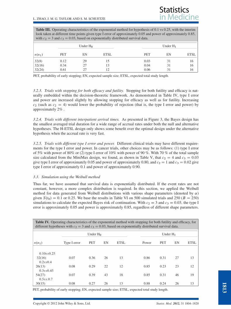
3.2.4. Trials with different interpatient arrival times. As presented in Figure 3, the Bayes design hasthe smallest averaged trial duration for a wide range of accrual rates under both the null and alternativehypotheses. The H-ETSL design only shows some benefit over the optimal design under the alternativehypothesis when the accrual rate is very fast.

3.2.5. Trials with different type I error and power. Different clinical trials may have different require-ments for the type I error and power. In cancer trials, other choices may be as follows: (1) type I errorof 5% with power of 80% or (2) type I error of 10% with power of 90 %. With 70 % of the total samplesize calculated from the MiniMax design, we found, as shown in Table V, that c2 D 4 and c3 D 0:03

give type I error of approximately 0.05 and power of approximately 0.80, and c2 D 1 and c3 D 0:02 givetype I error of approximately 0.1 and power of approximately 0.90.

3.3. Simulation using the Weibull method

Thus far, we have assumed that survival data is exponentially distributed. If the event rates are notconstant, however, a more complex distribution is required. In this section, we applied the Weibullmethod for data generated from Weibull distributions with various shape parameters (denoted by ˛)given S.t0/ D 0:1 or 0:25. We base the results in Table VI on 500 simulated trials and 250 (B D 250)simulations to calculate the expected Bayes risk of continuation. With c2 D 3 and c3 D 0:03; the type Ierror is approximately 0.05 and power is approximately 0.85, regardless of different shape parameters.

Table IV. Operating characteristics of the exponential method with stopping for both futility and efficacy, fordifferent hypotheses with c2 D 3 and c3 D 0:03, based on exponentially distributed survival data.

Under H0 Under H1

n.n1/ Type I error PET EN ETSL Power PET EN ETSL

0:10vs0:25

32(16) 0.07 0.36 26 13 0.86 0.31 27 130:2vs0:4

26(13) 0.08 0.29 22 12 0.85 0.23 23 120:3vs0:45

54(27) 0.07 0.39 43 18 0.85 0.31 46 190:5vs:0:7

30(15) 0.08 0.27 26 13 0.88 0.24 26 13



1813


0 10 20 30 40 50 60

010

2030

4050

6070

Inter−patient arrival time(days)

Exp

ecte

d T

rial D

urat

ion

unde

r H

0(m

onth

)

0 10 20 30 40 50 60

020

4060

8010

0

Inter−patient arrival time(days)Exp

ecte

d T

rial D

urat

ion

Und

er H

1(m

onth

)

H−ETSLOptimalBayes

(b)(a)

Figure 3. (a) Expected trial duration when S.t0/ D 0:1 for various interpatient arrival times; and (b) expectedtrial duration when S.t0/D 0:25 for various interpatient arrival times.

Table V. Operating characteristics of the exponential method, for different hypotheses with different type Ierror and power, based on exponentially distributed survival data.

Under H0 Under H1

Design n.n1/ Type I error PET EN ETSL Power PET EN ETSL

c2 D 4 and c3 D 0:03

0:1vs0:25

Optimal 43(18) 0.05 0.73 25 13 0.80 0.14 40 22Bayes 28(14) 0.05 0.29 24 12 0.80 0.04 27 150:2vs0:4

Optimal 43(13) 0.05 0.75 20 12 0.80 0.16 38 22Bayes 24(12) 0.05 0.24 21 12 0.79 0.03 24 140:3vs0:45

Optimal 82(30) 0.05 0.58 52 23 0.80 0.07 79 35Bayes 46(23) 0.05 0.33 39 17 0.82 0.05 45 210:5vs0:7

Optimal 43(15) 0.05 0.70 24 13 0.80 0.13 39 23Bayes 26(13) 0.04 0.19 24 13 0.81 0.02 26 14

c2 D 1 and c3 D 0:02

0:1vs0:25

Optimal 50(21) 0.10 0.67 31 15 0.90 0.07 48 24Bayes 28(14) 0.09 0.24 25 13 0.87 0.04 27 150:2vs0:4

Optimal 37(17) 0.10 0.56 26 15 0.90 0.05 36 21Bayes 26(13) 0.09 0.19 23 13 0.90 0.03 26 140:3vs0:45

Optimal 81(27) 0.10 0.59 51 23 0.90 0.07 78 34Bayes 50(25) 0.11 0.28 43 19 0.90 0.04 49 22

0:5vs0:7

Optimal 45(21) 0.10 0.66 29 15 0.90 0.07 43 24Bayes 28(14) 0.10 0.15 26 14 0.90 0.02 28 15


1814



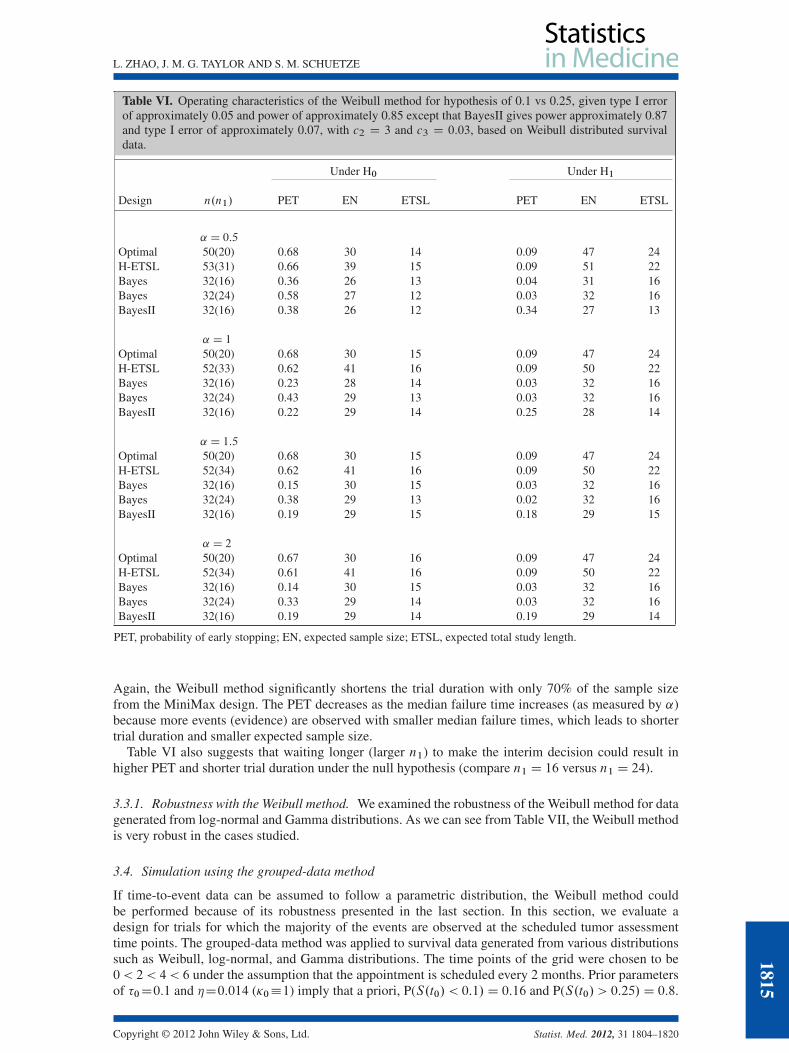
Table VI. Operating characteristics of the Weibull method for hypothesis of 0.1 vs 0.25, given type I errorof approximately 0.05 and power of approximately 0.85 except that BayesII gives power approximately 0.87and type I error of approximately 0.07, with c2 D 3 and c3 D 0:03, based on Weibull distributed survivaldata.

Under H0 Under H1

Design n.n1/ PET EN ETSL PET EN ETSL

˛ D 0:5

Optimal 50(20) 0.68 30 14 0.09 47 24H-ETSL 53(31) 0.66 39 15 0.09 51 22Bayes 32(16) 0.36 26 13 0.04 31 16Bayes 32(24) 0.58 27 12 0.03 32 16BayesII 32(16) 0.38 26 12 0.34 27 13

˛ D 1


˛ D 1:5


˛ D 2



Again, the Weibull method significantly shortens the trial duration with only 70% of the sample sizefrom the MiniMax design. The PET decreases as the median failure time increases (as measured by ˛)because more events (evidence) are observed with smaller median failure times, which leads to shortertrial duration and smaller expected sample size.

Table VI also suggests that waiting longer (larger n1) to make the interim decision could result inhigher PET and shorter trial duration under the null hypothesis (compare n1 D 16 versus n1 D 24).

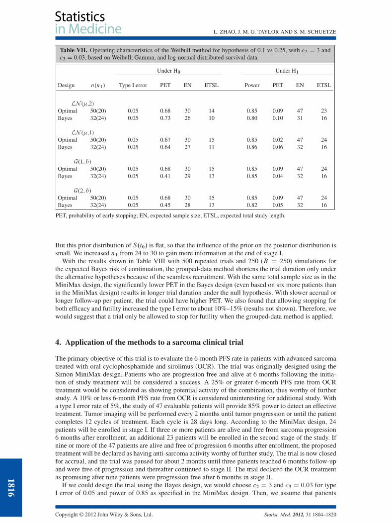
3.3.1. Robustness with the Weibull method. We examined the robustness of the Weibull method for datagenerated from log-normal and Gamma distributions. As we can see from Table VII, the Weibull methodis very robust in the cases studied.

3.4. Simulation using the grouped-data method

If time-to-event data can be assumed to follow a parametric distribution, the Weibull method couldbe performed because of its robustness presented in the last section. In this section, we evaluate adesign for trials for which the majority of the events are observed at the scheduled tumor assessmenttime points. The grouped-data method was applied to survival data generated from various distributionssuch as Weibull, log-normal, and Gamma distributions. The time points of the grid were chosen to be0 < 2 < 4 < 6 under the assumption that the appointment is scheduled every 2 months. Prior parametersof �0D0:1 and �D0:014 ( 0�1) imply that a priori, P(S.t0/ < 0:1/D 0:16 and P(S.t0/ > 0:25/D 0:8.


1815


Table VII. Operating characteristics of the Weibull method for hypothesis of 0.1 vs 0.25, with c2 D 3 andc3 D 0:03, based on Weibull, Gamma, and log-normal distributed survival data.

Under H0 Under H1

Design n.n1/ Type I error PET EN ETSL Power PET EN ETSL

LN (�,2)Optimal 50(20) 0.05 0.68 30 14 0.85 0.09 47 23Bayes 32(24) 0.05 0.73 26 10 0.80 0.10 31 16

LN (�,1)Optimal 50(20) 0.05 0.67 30 15 0.85 0.02 47 24Bayes 32(24) 0.05 0.64 27 11 0.86 0.06 32 16

G.1; b/Optimal 50(20) 0.05 0.68 30 15 0.85 0.09 47 24Bayes 32(24) 0.05 0.41 29 13 0.85 0.04 32 16

G.2; b/Optimal 50(20) 0.05 0.68 30 15 0.85 0.09 47 24Bayes 32(24) 0.05 0.45 28 13 0.82 0.05 32 16


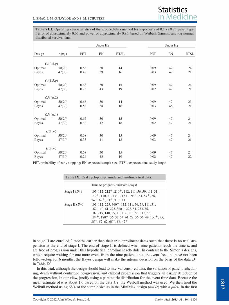
But this prior distribution of S.t0/ is flat, so that the influence of the prior on the posterior distribution issmall. We increased n1 from 24 to 30 to gain more information at the end of stage I.

With the results shown in Table VIII with 500 repeated trials and 250 (B D 250) simulations forthe expected Bayes risk of continuation, the grouped-data method shortens the trial duration only underthe alternative hypotheses because of the seamless recruitment. With the same total sample size as in theMiniMax design, the significantly lower PET in the Bayes design (even based on six more patients thanin the MiniMax design) results in longer trial duration under the null hypothesis. With slower accrual orlonger follow-up per patient, the trial could have higher PET. We also found that allowing stopping forboth efficacy and futility increased the type I error to about 10%–15% (results not shown). Therefore, wewould suggest that a trial only be allowed to stop for futility when the grouped-data method is applied.

4. Application of the methods to a sarcoma clinical trial

The primary objective of this trial is to evaluate the 6-month PFS rate in patients with advanced sarcomatreated with oral cyclophosphamide and sirolimus (OCR). The trial was originally designed using theSimon MiniMax design. Patients who are progression free and alive at 6 months following the initia-tion of study treatment will be considered a success. A 25% or greater 6-month PFS rate from OCRtreatment would be considered as showing potential activity of the combination, thus worthy of furtherstudy. A 10% or less 6-month PFS rate from OCR is considered uninteresting for additional study. Witha type I error rate of 5%, the study of 47 evaluable patients will provide 85% power to detect an effectivetreatment. Tumor imaging will be performed every 2 months until tumor progression or until the patientcompletes 12 cycles of treatment. Each cycle is 28 days long. According to the MiniMax design, 24patients will be enrolled in stage I. If three or more patients are alive and free from sarcoma progression6 months after enrollment, an additional 23 patients will be enrolled in the second stage of the study. Ifnine or more of the 47 patients are alive and free of progression 6 months after enrollment, the proposedtreatment will be declared as having anti-sarcoma activity worthy of further study. The trial is now closedfor accrual, and the trial was paused for about 2 months until three patients reached 6 months follow-upand were free of progression and thereafter continued to stage II. The trial declared the OCR treatmentas promising after nine patients were progression free after 6 months in stage II.

If we could design the trial using the Bayes design, we would choose c2 D 3 and c3 D 0:03 for typeI error of 0.05 and power of 0.85 as specified in the MiniMax design. Then, we assume that patients

1816



Table VIII. Operating characteristics of the grouped-data method for hypothesis of 0.1 vs 0.25, given typeI error of approximately 0.05 and power of approximately 0.85, based on Weibull, Gamma, and log-normaldistributed survival data.

Under H0 Under H1

Design n.n1/ PET EN ETSL PET EN ETSL

W(0.5,� )Optimal 50(20) 0.68 30 14 0.09 47 24Bayes 47(30) 0.48 39 16 0.03 47 21

W(1.5,� )Optimal 50(20) 0.68 30 15 0.09 47 24Bayes 47(30) 0.25 43 19 0.02 47 21

LN (�,2)Optimal 50(20) 0.68 30 14 0.09 47 23Bayes 47(30) 0.53 38 16 0.03 46 21

LN (�,1)Optimal 50(20) 0.67 30 15 0.09 47 24Bayes 47(30) 0.32 42 18 0.02 47 21

G.1; b/Optimal 50(20) 0.68 30 15 0.09 47 24Bayes 47(30) 0.33 41 18 0.03 47 21

G.2; b/Optimal 50(20) 0.68 30 15 0.09 47 24Bayes 47(30) 0.24 43 19 0.02 47 22


Table IX. Oral cyclophosphamide and sirolimus trial data.

Time to progression/death (days)

Stage I (D1) 103; 112; 212C; 210C; 112; 111; 56; 59; 111; 31;

142C; 110; 61; 133C; 133C; 93C; 51; 87C; 56;

74C; 67C; 53C; 31C; 11

Stage II (D2) 103; 112; 225; 360C; 112; 111; 56; 59; 111; 31;

162; 110; 61; 223; 360C; 225; 51; 253; 56;

107; 219; 140; 55; 11; 112; 113; 53; 112; 56;

184C; 180C; 56; 57; 54; 61; 28; 56; 56; 49; 100C; 95;

85C; 52; 62; 65C; 56; 42C

in stage II are enrolled 2 months earlier than their true enrollment dates such that there is no trial sus-pension at the end of stage I. The end of stage II is defined when nine patients reach the time t0 andare free of progression under this hypothetical enrollment schedule. In contrast to the Simon’s designs,which require waiting for one more event from the nine patients that are event free and have not beenfollowed-up for 6 months, the Bayes design will make the interim decision on the basis of the data D1in Table IX.

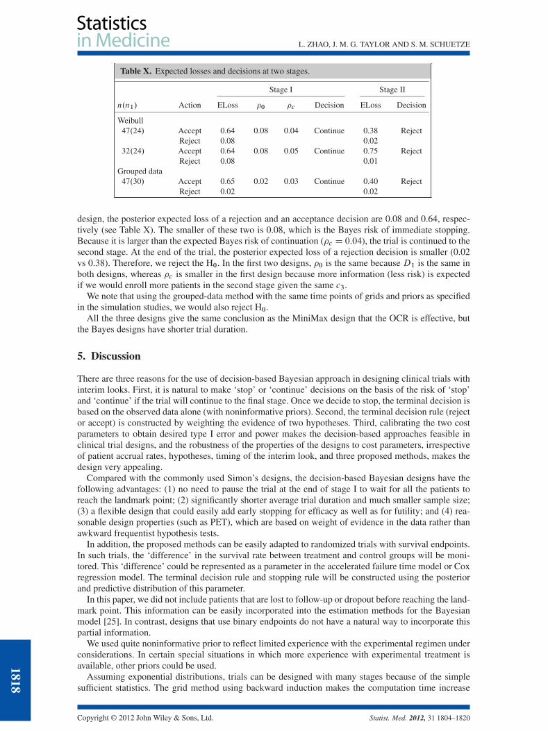
In this trial, although the design should lead to interval censored data, the variation of patient schedul-ing, death without confirmed progression, and clinical progression that triggers an earlier detection ofthe progression, in our view, justify using a parametric distribution for the event time data. Because themean estimate of ˛ is about 1.6 based on the data D1, the Weibull method was used. We then tried theWeibull method using 68% of the sample size as in the MiniMax design (nD32) with n1D24. In the first


1817


Table X. Expected losses and decisions at two stages.

Stage I Stage II

n.n1/ Action ELoss �0 �c Decision ELoss Decision

Weibull47.24/ Accept 0.64 0.08 0.04 Continue 0.38 Reject

Reject 0.08 0.0232.24/ Accept 0.64 0.08 0.05 Continue 0.75 Reject

Reject 0.08 0.01Grouped data47.30/ Accept 0.65 0.02 0.03 Continue 0.40 Reject

Reject 0.02 0.02

design, the posterior expected loss of a rejection and an acceptance decision are 0.08 and 0.64, respec-tively (see Table X). The smaller of these two is 0.08, which is the Bayes risk of immediate stopping.Because it is larger than the expected Bayes risk of continuation (�c D 0:04), the trial is continued to thesecond stage. At the end of the trial, the posterior expected loss of a rejection decision is smaller (0.02vs 0.38). Therefore, we reject the H0. In the first two designs, �0 is the same because D1 is the same inboth designs, whereas �c is smaller in the first design because more information (less risk) is expectedif we would enroll more patients in the second stage given the same c3.

We note that using the grouped-data method with the same time points of grids and priors as specifiedin the simulation studies, we would also reject H0.

All the three designs give the same conclusion as the MiniMax design that the OCR is effective, butthe Bayes designs have shorter trial duration.

5. Discussion

There are three reasons for the use of decision-based Bayesian approach in designing clinical trials withinterim looks. First, it is natural to make ‘stop’ or ‘continue’ decisions on the basis of the risk of ‘stop’and ‘continue’ if the trial will continue to the final stage. Once we decide to stop, the terminal decision isbased on the observed data alone (with noninformative priors). Second, the terminal decision rule (rejector accept) is constructed by weighting the evidence of two hypotheses. Third, calibrating the two costparameters to obtain desired type I error and power makes the decision-based approaches feasible inclinical trial designs, and the robustness of the properties of the designs to cost parameters, irrespectiveof patient accrual rates, hypotheses, timing of the interim look, and three proposed methods, makes thedesign very appealing.

Compared with the commonly used Simon’s designs, the decision-based Bayesian designs have thefollowing advantages: (1) no need to pause the trial at the end of stage I to wait for all the patients toreach the landmark point; (2) significantly shorter average trial duration and much smaller sample size;(3) a flexible design that could easily add early stopping for efficacy as well as for futility; and (4) rea-sonable design properties (such as PET), which are based on weight of evidence in the data rather thanawkward frequentist hypothesis tests.

In addition, the proposed methods can be easily adapted to randomized trials with survival endpoints.In such trials, the ‘difference’ in the survival rate between treatment and control groups will be moni-tored. This ‘difference’ could be represented as a parameter in the accelerated failure time model or Coxregression model. The terminal decision rule and stopping rule will be constructed using the posteriorand predictive distribution of this parameter.

In this paper, we did not include patients that are lost to follow-up or dropout before reaching the land-mark point. This information can be easily incorporated into the estimation methods for the Bayesianmodel [25]. In contrast, designs that use binary endpoints do not have a natural way to incorporate thispartial information.

We used quite noninformative prior to reflect limited experience with the experimental regimen underconsiderations. In certain special situations in which more experience with experimental treatment isavailable, other priors could be used.

Assuming exponential distributions, trials can be designed with many stages because of the simplesufficient statistics. The grid method using backward induction makes the computation time increase

1818



linearly with the number of stages. However, the Weibull and grouped-data methods are practically lim-ited to two stages mainly because there are not a small number of sufficient statistics [30, 31]. For thesetwo methods, Bayes risk was calculated in a forward fashion, for which the computation time increaseexponentially with the number of stages, which makes adding one more interim look computationallyinfeasible although theoretically possible.

In summary, Bayesian decision-based approaches are feasible in designing clinical trials with appeal-ing properties. As more and more experience accumulates with the application of this approach in realtrials, it may be possible to design the trials by directly specifying the costs rather than treating them astuning parameters.

Acknowledgements

Many thanks to Frank E. Harrell for his encouragement to initiate this research. The authors gratefullyacknowledge the constructive comments of an associate editor and referees.

References1. Chan JK, Ueda SM, Sugiyama VE, et al. 578 Analysis of phase II studies on targeted agents and subsequent phase III

trials: what are the 579 predictors for success? J Clin Oncol 2008; 26:1511–1518.2. Korn EL, Arbuck SG, Pluda JM, et al. Clinical trial designs for cytostatic agents: are new approaches needed? J Clin

Oncol 2001; 19:265–72.3. Stone A, Wheeler C, Barge A. Improving the design of phase II trials of cytostatic anticancer agents. Contemporary

Clinical Trials 2007; 28:138–145.4. Panageas KS, Ben-Porat L, Dickler MN, et al. When you look matters: the effect of assessment schedule on

progression-free survival. J Natl Cancer Inst 2007; 99:428–32.5. Gehan EA. The determination of the number of patients required in a preliminary and a follow up 555 trial of a new

chemotherapeutic agent. J Chronic Dis 1961; 13:346–353.6. Fleming TR. One-sample multiple testing procedure for phase II clinical trials. Biometrics 1982; 38(558):143–151.7. Simon R. Optimal two-stage designs for phase II clinical trials. Controlled Clinical Trials 1989; 10:1–10.8. Herndon JE. A design alternative for two-stage, phase II, multicenter cancer clinical. Contemporary Clinical Trials 1998;

19(5):440–450.9. Case LD, Morgan TM. Design of Phase II cancer trials evaluating survival probabilities. BMC Medical Research

Methodology 2003; 3:6. DOI: 10.1186/1471-2288-3-6.10. Lin DY, Shen L, Ying Z, Breslow NE. Group sequential designs for monitoring survival probabilities. Biometrics 1996;

52:1033–1041. DOI: 10.1200/JCO.2009.22.4329.11. Huang B, Talukder E, Thomas N. Optimal two-stage phase II designs with long-term endpoints. American Statistical

Association, Statsitics in Biopharmaceutical Research 2010; 2:51–60. DOI: 10.1198/sbr.2010.09001.12. Follman DA, Albert PS. Bayesian monitoring of event rates with censored data. Biometrics 1999; 55(2):603–607.13. Rosner GL. Bayesian monitoring of clinical trials with failure-time endpoint. Biometrics 2005; 61:239–245.14. Cheung YK, Thall PF. Monitoring the rates of composite events with censored data in phase II clinical trials. Biometrics

2002; 58:89–97.15. Thall PF, Wooten LH, Tannir NM. Monitoring event times in early phase clinical trials: some practical issues. Clin Trials

2005; 2(6):467–78.16. Thall PF, Simon R, Estey EH. Bayesian sequential monitoring designs for single-arm clinical trials with multiple

outcomes. Statistics in Medicine 1995; 14:357–379.17. Lachin J. A review of methods for futility stopping based on conditional power. Statistics in Medicine 2005; 24:

2747–2764. DOI: 10.1002/sim.2151.18. Pepe MS, Anderson GL. Two-stage experimental designs: early stopping with a negative result. Applied Statistics 1992;

41:181–190.19. Berry DA. Bayesian clinical trials. Nature Reviews Drug Discovery 2006; 5:27–36. DOI: 10.1038/nrd1927.20. Staquet MJ, Sylvester RJ. A decision theory approach to phase II clinical trials. Biomedicine 1977; 26(4):262–266.21. Sylvester RJ, Staquet MJ. Design of phase II clinical trials in cancer using decision theory. Cancer Treatment Report 1980;

64(2-3):519–524.22. Sylvester RJ. A Bayesian approach to the design of phase II clinical trials. Biometrics 1988; 44(3):823–836.23. Brunier HC, Whitehead J. Sample sizes for phase II clinical trials derived from Bayesian decision theory. Statistics in

Medicine 1994; 13(23-24):2493–2502.24. Stallard N. Sample size determination for phase II clinical trials based on Bayesian decision theory. Biometrics 1998;

54(1):279–294.25. Zhao L, Woodworth G. Bayesian decision sequential analysis with survival endpoint in phase II clinical trials. Statistics

in Medicine 2009; 28:1339–1352. DOI: 10.1002/sim.3544.26. Berry SM, Carlin BP, Lee J, Muller P. Bayesian Adaptive Methods for Clinical Trials, Chapman & Hall/ CRC Biostatistics

Series. Boca Raton: CRC Press, 2011.27. Albert J. Bayesian Computation with R. Springer: New York, 2009.


1819


28. Kalbfleisch J. Nonparametric Bayesian analysis of survival time data. Journal of the Royal Statistical Society 1978;40:214–221.

29. Ibrahim JG, Chen MH, Sinha D. Bayesian Survival Analysis. Springer: New York, 2001. 50–53.30. Muller P, Berry DA, Grieve AP, et al. Simulation-based sequential Bayesian design. Journal of Statistical Planning and

Inference 2007; 137(10):3140–3150. DOI: 10.1016/j.jspi.2006.05.021.31. Brockwell AE, Kadane JB. Sequential analysis by griding sufficient statistics. J. Comput. Graph. Statist 2003; 12:566–584.

1820


Documents

Bayesian decision theoretic two-stage design in phase II