Bayesian Catch Curve AnalysisInstitute of Statistics Mimeo Series # 2615

Emily H. Griffith1,5, Sujit K. Ghosh1, Kenneth H. Pollock3, and Michael J.Seider4

1Department of StatisticsNorth Carolina State UniversityRaleigh, NC 27695

3Department of ZoologyNorth Carolina State UniversityRaleigh, NC 27695

4Lake Superior Fisheries TeamWisconsin Department of Natural ResourcesP.O. Box 589141 South Third StreetBayfield, WI 54814

5Corresponding author:Patuxent Wildlife Research Center12100 Beech Forest Road, G-2Laurel, MD 20708egriffith@usgs.gov

1

Abstract

Catch curves have been used to estimate survival and instantaneous mortality for

fish and wildlife populations for many years. In order to better analyze catch

curve data from the Apostle Islands population lake trout Salvelinus namaycush

in Lake Superior, we develop a Bayesian approach to catch curve analysis. First,

the proposed Bayesian approach is illustrated for a single catch curve and then

extended to multiple years of data. We also relax the model assumption of a

stable age distribution to allow random effects across years. The proposed models

are compared with the traditional methods using the focused DIC. There are many

potential advantages to the Bayesian approach over the traditional methods such

as least squares and maximum likelihood, based on large sample theory. Bayesian

estimates are valid for finite samples, and efficient numerical methods can be used

to obtain estimates of instantaneous mortality. We conclude that many benefits can

be obtained from the Bayesian approach to a single catch curve and to multiple

years of data, such as closed-form variance estimates and the ability to both model

and estimate the process variation of survival rates.

Key words: Focused DIC; Life table methods; Markov chain Monte Carlo meth-

ods; Standing age distribution; Survival estimation.

1 Introduction

Lake trout Salvelinus namaycush from the Apostle Islands population in Lake

Superior are recovering from both overfishing and predation by sea lampreys

2

Petromyzon marinus (Linton et al. 2007; Pollock et al. 2007). Due to the im-

portance of lake trout, both economically and ecologically, monitoring the popu-

lations’ demographic parameters is crucial. Linton et al. (2007) analyze age dis-

tribution and catch-per-unit-effort data, while Pollock et al. (2007) analyze mark-

recapture data from this population. We obtained a set of catch curves, collected

on male lake trout from 1986 through 2005 (unpublished data collected by the

Wisconsin Department of Natural Resources). Catch curves tend to be both inex-

pensive and simple to collect, but their usefulness is limited by strict assumptions

regarding population dynamics. Our objective is to utilize Bayesian inference to

better use this type of data.

Chapman and Robson (1960) and Robson and Chapman (1961) formally de-

veloped statistical methods of analyzing catch curve data. They proposed es-

timating the survival probability, denoted by S, by using a regression model, a

geometric model, and a multinomial model. The regression model is based on the

idea that E(nx) = NS1S2S3 . . .Sx p where Sx denotes the survival probability of an

individual at age x, N the total number of individuals, p the capture probability,

and nx is the number of fishes captured from age class x. If capture probability

(p) and survival rate (S) are age independent, then it follows that E(nx) = NSx p

(Seber 1982, p. 426). Thus, in a linear regression relating lognx to x, the slope of

the line is logS (Chapman and Robson 1960). This can be used as an approximate

model, where the variance being dependent on age is ignored. Both Chapman and

Robson (1960) and Seber (1982) recommend truncating the catch curve data at

the point where nx drops below 5 in order to reduce the dependence of σ2 on x.

3

Chapman and Robson (1960) also developed methods to use the geometric

distribution and the multinomial distribution to obtain a maximum likelihood es-

timator and then a uniformly minimum variance unbiased estimator (UMVUE)

of the survival rate. The assumptions for the Chapman-Robson survival estimate

are constant survival for all age classes and all years, a stable age distribution, a

stationary population, and equal catchability for all fully vulnerable age classes.

A population with a stable age distribution has survival and fecundity rates that

have remained constant for a long period of time (Messier 1990; Udevitz and Bal-

lachey 1998). However, a stable age distribution does not necessarily imply that

the population size remains constant. A population can increase, decrease, or re-

main constant in size and still have a stable age distribution (Williams et al. 2002).

A stationary population is one where the populations growth rate is one. Let Nx

be the number of individuals in the sample of age x. Also let T = ∑x xNx. Notice

that there exists a finite maximum age, xmax, such that Nx = 0 for all x > xmax and

hence T is finite with probability 1. The Nx’s conditional on ∑Nx = N follow a

multinomial distribution, given below.

L(S|N,T ) = P(N0 = n0,N1 = n1, . . . |N)

=N!

∏∞x=0 nx!

∞

∏x=0

(Sx)nx(1−S)N∝ ST (1−S)N . (1)

The maximum likelihood estimator (MLE) of S based on the above likelihood

is

SMLE = X/(1+ X), (2)

4

where X = T/N. The MLE is a biased estimator (Chapman and Robson 1960). A

uniformly minimum variance unbiased estimator (UMVUE) for S does exist, and

is given by the formula

SU =X

1+ X−( 1

N

) . (3)

The variance for SU cannot be obtained in closed form. The minimum variance

unbiased estimator of var(SU) is

var(SU) = SU

(SU −

T −1N +T −2

). (4)

Chapman and Robson (1960) also discuss the instantaneous mortality rate, Z,

which can be defined by the relationship Z = − logS. For the geometric model,

no unbiased estimate of Z exists (Chapman and Robson 1960). Z can be esti-

mated consistently using the fact that ZMLE = log(SMLE). Z can also be estimated

using least-squares estimation. However, Chapman and Robson (1960) do not

recommend using the regression estimator due to the potential for bias due to the

violation of the assumption of constant variance. Robson and Chapman (1961)

conclude that the best estimate for S, and the corresponding standard error, is the

UMVUE.

Jensen (1985) compares the UMVUE of S suggested by Chapman and Rob-

son (1960) and Robson and Chapman (1961) to the least-squares estimate. Jensen

(1985) concludes that the precision of the UMVUE is a function of the number of

animals in the catch curve. However, the precision of the least-squares estimate

of S increases with the number of age classes in the sample. Murphy (1997) also

5

explored the bias in the Chapman-Robson estimator of instantaneous mortality

from the UMVUE of S, SU , setting ZU = log(SU) and compared it with the bias

for the least-squares regression estimate of the same. Murphy (1997) found that

the least-squares regression estimates of Z were biased, underestimating the true

instantaneous mortality rate. Small samples and low instantaneous mortality in-

crease this bias (Murphy 1997). We conclude that the UMVUE of S has the most

desirable properties out of all these estimators. However, there is not a closed

form estimate of the variance of the survival rate parameter under the geometric

or multinomial model. Also, the UMVUE does not exist for estimating Z.

In this article we develop a Bayesian approach to estimate S and Z and we

show that closed form estimates can be obtained based on a finite sample. In

Section 2, we describe our method for a single catch curve analysis. In Section

4, we extend our method to multiple years of catch curves. In Section 6, we

extend our method further to allow for the survival rate to have a random effect

across years. In Sections 4 and 6, the methods are illustrated with analysis based

on real data. In Section 7, we report the results of two simulation studies that we

performed to test our random effects method. We conclude with some suggestions

for future research, in Section 8.

2 Bayesian Catch Curve with Conjugate Priors

We now present a Bayesian analysis using conjugate priors. The conjugate prior

for the multinomial distribution is the Dirichlet distribution (Robert 2001, p. 121).

6

In the specific case of the catch curve’s conditional multinomial distribution, be-

cause there are only two multinomial probabilities, S and 1−S, the Dirichlet dis-

tribution reduces to the Beta(α,β ) distribution (Robert 2001, p. 521).

Applying Bayes Theorem to the likelihood of the data given in Equation (1)

and the Beta(α,β ) prior distribution yields the posterior density

π(S|T,N,α,β ) =ST+α−1(1−S)N+β−1

B(T +α,N +β ), (5)

meaning that the posterior distribution of S is a Beta(T +α,N +β ) distribution.

The Bayes estimator of S under squared error loss is the posterior expectation

of the Beta(T +α,N +β ) distribution. Thus, the Bayes estimator of S is given by

SB = E[S|N,T ] =T +α

T +α +N +β, (6)

with corresponding variance

var(SB) = var[S|N,T ] =(T +α)(N +β )

(T +α +N +β )2(T +α +N +β +1). (7)

These results hold true for any α and β that satisfy T + α > 0 and N + β > 0.

Using specific α’s and β ’s, we can obtain the other estimators of the survival rate

using Bayesian inference. Notice that as α +β → 0, SB→ SMLE . Thus the MLE

can be obtained as a limiting case of the Bayes estimator using an improper prior

π(S) = 1/(S(1−S)). This prior has most of its weight at zero and one. Similarly,

as α → 0 and β →−1, SB→ SU and again we see that the UMVUE is obtained

7

as a limit of the Bayes estimator using an improper prior π(S) = 1/(S(1− S)2).

This prior has most of its weight at zero and one. Note that 1/(S(1− S)2)→ ∞

as S → 0 or S → 1. Alternatively, if we use the weighted squared error loss,

Lw(S,a) = w(S)(S− a)2 with w(S) = 1/(S(1− S)) then the Bayes estimator is

given by SwB = E(w(S)S|T,N)/E(w(S))|T,N) = SMLE if α = β = 1.

Bayesian inference calls for a prior distribution on the parameter S. If we

do not have any substantial prior information, we can use a noninformative prior

like the Jeffreys prior. Jeffreys prior is π∗(S) ∝ |I(S)|12 where I(S) is Fisher’s

information (Robert 2001, p. 130). Notice that I(S) = E[−∂ 2 logL(S|N,T )/∂S2]

= E[T/S2 +N/(1−S)2] = N/(S(1− S)2), which leads to Jeffreys prior being

π∗(S) ∝ [√

S(1−S)]−1, which is the limiting kernel of a Beta(1/2,β ) distribution

when β → 0. Thus, in this case the posterior distribution, using Jeffreys prior, is

a Beta(T +1/2,N), which is a proper distribution as long as N > 0.

Using Jeffreys prior, the posterior mean and variance of S are

SJ =T + 1

2

T +N + 12

(8)

and

var(SJ) =(T + 1

2)(N)(T +N + 1

2)2(T +N + 32)

, (9)

respectively.

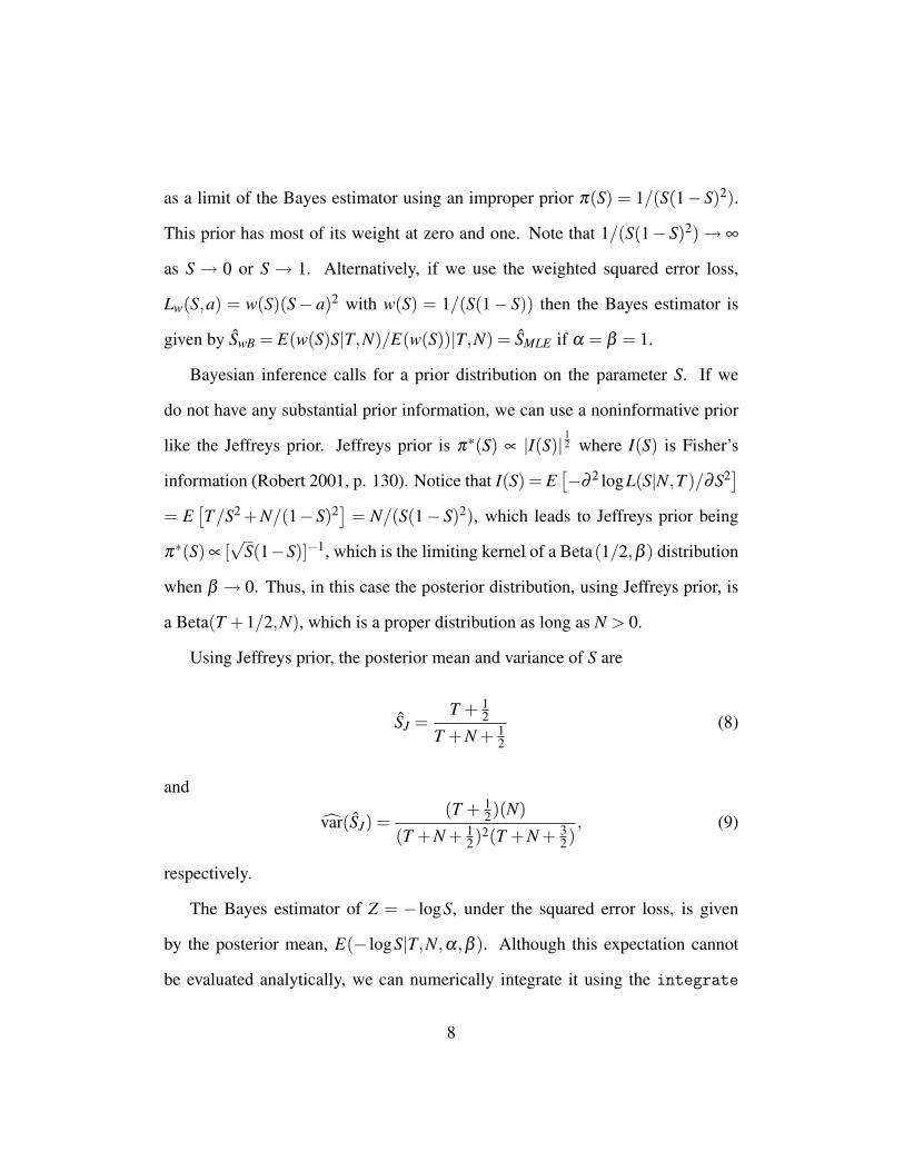
The Bayes estimator of Z = − logS, under the squared error loss, is given

by the posterior mean, E(− logS|T,N,α,β ). Although this expectation cannot

be evaluated analytically, we can numerically integrate it using the integrate

8

function available in the software R . Alternatively, we may use Monte Carlo

methods to numerically approximate ZB = E(− logS|T,N,α,β ).

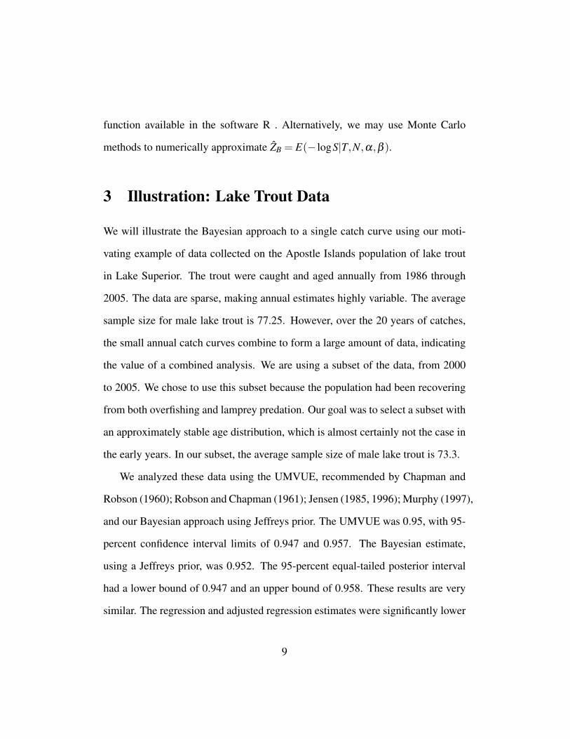
3 Illustration: Lake Trout Data

We will illustrate the Bayesian approach to a single catch curve using our moti-

vating example of data collected on the Apostle Islands population of lake trout

in Lake Superior. The trout were caught and aged annually from 1986 through

2005. The data are sparse, making annual estimates highly variable. The average

sample size for male lake trout is 77.25. However, over the 20 years of catches,

the small annual catch curves combine to form a large amount of data, indicating

the value of a combined analysis. We are using a subset of the data, from 2000

to 2005. We chose to use this subset because the population had been recovering

from both overfishing and lamprey predation. Our goal was to select a subset with

an approximately stable age distribution, which is almost certainly not the case in

the early years. In our subset, the average sample size of male lake trout is 73.3.

We analyzed these data using the UMVUE, recommended by Chapman and

Robson (1960); Robson and Chapman (1961); Jensen (1985, 1996); Murphy (1997),

and our Bayesian approach using Jeffreys prior. The UMVUE was 0.95, with 95-

percent confidence interval limits of 0.947 and 0.957. The Bayesian estimate,

using a Jeffreys prior, was 0.952. The 95-percent equal-tailed posterior interval

had a lower bound of 0.947 and an upper bound of 0.958. These results are very

similar. The regression and adjusted regression estimates were significantly lower

9

than both the Bayes estimate and the UMVUE. The bias that we found is the same

as the bias found in Jensen (1996).

These estimates of the survival rate are all high (above 0.90), indicating low

mortality. The data were collected during a spawning survey where larger fish

tend to be collected. These larger fish may experience higher survival rates due

to an increased ability to survive a lamprey attack and lowered vulnerability to

commercial and recreational fishing gears (M. Seider, personal communication,

June 20, 2008).

4 Bayesian Catch Curve with Multiple

Years of Data

The catch curve estimates by Chapman and Robson (1960) require the assump-

tions that the age distribution is stable and stationary and survival is constant for

all age classes. It is also assumed that the ages are sampled randomly above some

minimum age. If we can justify these assumptions, combining catch data over

multiple years will result in a more precise estimate of the constant survival rate

due to the increase in sample size. The likelihood function for k years of catch-

curve data, assuming independence, is given by

L(S|N1,N2, . . . ,Nk,T1,T2, . . . ,Tk) ∝ ST1+T2+···+Tk(1−S)N1+N2+···+Nk (10)

Using the conjugate prior, which remains the Beta(α ,β ) distribution, the pos-

10

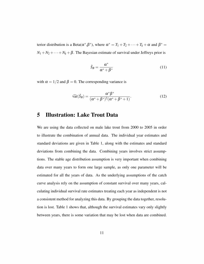
terior distribution is a Beta(α∗,β ∗), where α∗ = T1 + T2 + · · ·+ Tk + α and β ∗ =

N1 +N2 + · · ·+Nk +β . The Bayesian estimate of survival under Jeffreys prior is

SB =α∗

α∗+β ∗(11)

with α = 1/2 and β = 0. The corresponding variance is

var(SB) =α∗β ∗

(α∗+β ∗)2(α∗+β ∗+1). (12)

5 Illustration: Lake Trout Data

We are using the data collected on male lake trout from 2000 to 2005 in order

to illustrate the combination of annual data. The individual year estimates and

standard deviations are given in Table 1, along with the estimates and standard

deviations from combining the data. Combining years involves strict assump-

tions. The stable age distribution assumption is very important when combining

data over many years to form one large sample, as only one parameter will be

estimated for all the years of data. As the underlying assumptions of the catch

curve analysis rely on the assumption of constant survival over many years, cal-

culating individual survival rate estimates treating each year as independent is not

a consistent method for analyzing this data. By grouping the data together, resolu-

tion is lost. Table 1 shows that, although the survival estimates vary only slightly

between years, there is some variation that may be lost when data are combined.

11

This leads us to a better model which we develop in the next section.

6 Random Effects Model for Multiple Years of Data

If we consider the possibility that the survival rate is a random effect with a con-

stant mean and some variance, we can use multiple years of catch curve data to

estimate the mean and variance of the random effect process. The estimates ob-

tained will be ecologically meaningful, as there is often some natural temporal

variation in the survival rates of a population. Now we assume that survival is

constant for all age classes but is a function of a random process with a constant

mean and variance for all years. Each catch curve will provide a point estimate of

survival at that time. Combining years of data will provide estimates of the mean

and variance of the random process.

In a Bayesian framework, we can modify the likelihood given in Equation (10)

to allow for S to vary with year k. The likelihood will then be a product of the

likelihoods for each year, given below.

L(S1, . . . ,Sk|N1, . . . ,Nk,T1, . . . ,Tk) =k

∏j=1

L(S j|N j,Tj) ∝

k

∏j=1

STjj (1−S j)N j (13)

If we assign the random effect S j a Beta(τS∗,τ(1−S∗)) distribution, each S j

will have population mean S∗ and population variance S∗(1− S∗)/(τ + 1). Be-

cause we do not know S∗ or τ , we can use the Bayesian hierarchical framework

and assign S∗ a Beta(α,β ) prior and τ a Gamma(a,b) prior. We set α = β = .5

12

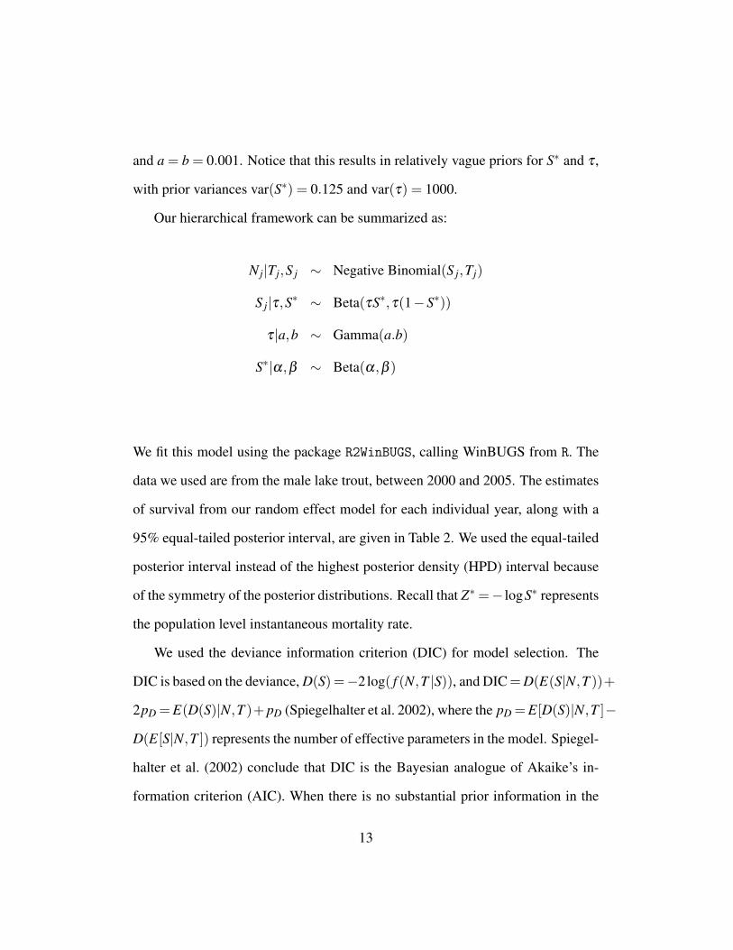
and a = b = 0.001. Notice that this results in relatively vague priors for S∗ and τ ,

with prior variances var(S∗) = 0.125 and var(τ) = 1000.

Our hierarchical framework can be summarized as:

N j|Tj,S j ∼ Negative Binomial(S j,Tj)

S j|τ,S∗ ∼ Beta(τS∗,τ(1−S∗))

τ|a,b ∼ Gamma(a.b)

S∗|α,β ∼ Beta(α,β )

We fit this model using the package R2WinBUGS, calling WinBUGS from R. The

data we used are from the male lake trout, between 2000 and 2005. The estimates

of survival from our random effect model for each individual year, along with a

95% equal-tailed posterior interval, are given in Table 2. We used the equal-tailed

posterior interval instead of the highest posterior density (HPD) interval because

of the symmetry of the posterior distributions. Recall that Z∗=− logS∗ represents

the population level instantaneous mortality rate.

We used the deviance information criterion (DIC) for model selection. The

DIC is based on the deviance, D(S)=−2log( f (N,T |S)), and DIC = D(E(S|N,T ))+

2pD = E(D(S)|N,T )+ pD (Spiegelhalter et al. 2002), where the pD = E[D(S)|N,T ]−

D(E[S|N,T ]) represents the number of effective parameters in the model. Spiegel-

halter et al. (2002) conclude that DIC is the Bayesian analogue of Akaike’s in-

formation criterion (AIC). When there is no substantial prior information in the

13

model, the DIC is approximately equal to the AIC. Spiegelhalter et al. (2002)

discuss one benefit of the DIC over model selection criteria such as the AIC or

the Bayes information criterion (BIC), which is that the BIC and AIC involve the

specification of the number of parameters in the model. The number of parame-

ters is not always easily determined in a hierarchical model, especially those that

involve random effects.

In Table 2, we present the posterior mean and standard deviation of the ran-

dom effects (S j’s) and from column 3 of this table it is clear that the variance

components are relatively small as all the posterior standard deviations of the S j’s

are smaller than 0.01. The deviance information criterion, or DIC, of the random

effect model is 46.3, which is larger than the DIC of the constant S model for

the same data, which is 43.6 (see Table 1). This implies that the random effect

model is not an improvement for this particular dataset. However, the DIC of the

random effect model, 46.3, is smaller than that of the individual yearly estimates

(fixed effect model), which was 49.2 (see Table 1). The random effect model is an

improvement over estimating each year separately for this dataset. Overall, being

able to relax the assumption of constant survival and implement a random effects

model is an improvement to the analysis of catch curve data, as it adds to the in-

formation gained from the analysis, whether that model is the best-fitting model

or not.

The traditional DIC focuses on the posterior distribution, not the level of

the hierarchy where the difference between the random effects model and the

constant survival model lies. The focused DIC (Bob O’Hara, personal website,

14

http://deepthoughtsandsilliness.blogspot.com/2007/12/focus-on-dic.html, Decem-

ber 5, 2007) looks at the marginal deviance instead of the traditional conditional

deviance.

The marginal distribution of N and T for the random effects model is

m(N,T |S∗,τ) =∫ 1

S j=0∏

j

(N j +Tj−1

Tj

)STj

j (1−S j)N j

×SτS∗−1

j (1−S j)τ(1−S∗)−1

B(τS∗,τ(1−S∗))dS j

= ∏j

(N j +Tj−1

Tj

)B(Tj + τS∗,N j + τ(1−S∗)

B(τS∗,τ(1−S∗)). (14)

The focused DIC, or fDIC, uses the focused deviance. The focused deviance is

defined as D f (S∗,τ) =− log(m(N,T |S∗,τ)). The fDIC can be defined as

f DIC = D f (S∗, τ)+2p fD (15)

where p fD = E(D f (S∗,τ)|N,T )−D f (S∗, τ) and S∗ and τ represent the posterior

mean of S∗ and τ , respectively. The focused DIC is only appropriate to calculate

in the presence of a random effect, but it can be compared with the traditional DIC

for model selection between models with and without random effects.

The focused DIC for the random effects model is 75.3, with p fD = 2. The fixed

effects model is clearly selected, since the DIC for the fixed model is 43.6, with

pD = 1. The variation between years is small, indicating that the extra parameters

15

to account for such a small random effect are not necessary to explain the yearly

variations. In order to more formally explore the use of fDIC as a model selection

tool we perform a simulation study.

7 Simulation Studies

As it is likely that survival rates will vary between years in other real fish as

wildlife populations, we were interested in seeing what happens to standard es-

timates of survival when the survival rate is constant for all ages, but varies

randomly from year to year. We examined survival rates of S = 0.6, 0.75 and

0.9 combined with random effects generated from a Normal(0,σ) distribution

with σ = 0, 0.05, and 0.25. We added random variation to them using the for-

mula logit(Si) = logit(S) + ηi, or Si = ( S1−S)eηi

1+( S1−S)eηi

, where ηi is generated from a

Normal(0,σ) distribution. We know that nx ∼ Binomial(N0,∏xi=1 Si), so we gen-

erated catch curve data by randomly generating the number of animals caught in

each age class using the Binomial distribution. Using σ = 0.25 means that the

range of values within two standard deviations is 0.24, 0.19, and 0.09 for survival

rates of 0.6, 0.75, and 0.9, respectively.

We generated 10,000 single catch curves with 50 age classes for each combi-

nation, setting the number of animals in our sample and in the zero age class, N0,

equal to 100. We estimated the survival rate, S, and the corresponding standard

deviation, σS, using the UMVUE and the Bayesian estimator with Jeffreys prior.

The results are given in Table 3.

16

The results show that, despite the addition of random variation, the point es-

timate from a single catch curve remains unbiased. These models appear to be

very robust against the random effect in the estimation of the survival rate, S, as

long as the age distribution is stable. The variance estimates underestimate the

true amount of variability in the population. This can be seen by comparing the

mean estimates of the standard deviation of S with the standard deviation of the

estimates of S.

We also carried out a separate simulation study to judge how well the focused

DIC performed at selecting the correct model in the presence of a random effect

compared to the traditional DIC.

For this simulation study, we examined two survival rates and four levels of

variability. We set S∗ = 0.6 or 0.8 and√

S∗(1−S∗)/(τ +1) = 0, 0.05, 0.10, and

0.20. We used a Beta(τS∗,τ(1− S∗)) distribution to generate the survival rates

with the random effect. We generated 6 years of catch curve data 1,000 times

and fit both the fixed effect and random effect model to each. The corresponding

results are given in Table 4.

The pD estimate is good under the fixed effect model. The focused DIC se-

lected the fixed effects model correctly much more frequently than the traditional

DIC. The focused DIC tended to select the fixed effects model more often than

the traditional DIC in all cases, but it did select the random effects model more

often as the size of the random effect increased. There was a huge increase in

performance between the fDIC and the DIC when the fixed model was the correct

model.

17

The probability of a Type I error, Pr[Reject H0|H0,σ = 0], when S = 0.8 is

0.52 for the fDIC and 0.96 for the DIC. When S = 0.6, the probability of a Type I

error is 0.37 for the fDIC and 0.82 for the DIC. Table 4 also gives the probabilities

of a Type II error, Pr[Fail to reject H0|HA], for σ = 0.05, 0.10, and 0.20 and

S = 0.8 and 0.6. In terms of total error, the sum of Type I and Type II error, for each

level of S and σ , it appears that fDIC outperforms DIC. This suggests that when

the focused DIC can be calculated, it is a good improvement over the traditional

DIC for model selection involving both fixed and random effect models.

8 Conclusions

For a single catch curve, the MLE and the least-squares estimators of the survival

rate are biased, but for the MLE, the bias reduces to zero as the sample size ap-

proaches infinity (Chapman and Robson 1960; Jensen 1985, 1996; Murphy 1997;

Dunn et al. 2002). For the UMVUE, there is no closed form estimate of the vari-

ance of the survival rate parameter(s) under the geometric or multinomial model.

Using Bayesian analysis, we can obtain a closed form finite sample estimate of the

survival rate(s) as well as a closed form estimate of its variance. It is also straight-

forward to obtain the Bayesian estimate of the instantaneous mortality rate Z.

We analyzed catch curve data from the Apostle Islands population of lake trout

in Lake Superior (Pollock et al. 2007) and found that our closed form Bayesian es-

timate performed very similar to the UMVUE when Jeffreys prior is used. We also

explored analytic relationships between the Bayesian estimator and the UMVUE

18

and MLE and showed that the latter estimates can be obtained as a limiting case

of Bayes estimates.

To extend our model, we considered the situation where multiple years of

catch data are collected. We first combined the separate years of data which,

under the assumptions of the Chapman and Robson (1960) estimator, results in

increased precision. However, information about possible assumption violations

is lost, because no information about the individual years is part of this model. We

relaxed the assumptions of Chapman and Robson (1960) and fit a random effects

model to multiple years of catch data. The random effects model is an important

advance because many real populations are likely to have substantial variation in

survival rates between years due to environmental perturbations. The focused DIC

also appears to be a good advance for model selection between fixed and random

effects models.

The Bayesian approach to catch curve data analysis provides a broad and flex-

ible method to extract the most information from the data without having to use

marked animals. This is a real benefit for studies of animals that are difficult to

mark. Bayesian methods are a very useful tool for data analysis. With software

like WinBUGS and R widely available and free to use, we think these methods

should become more popular in mainstream fisheries journals and in practice.

Acknowledgments

We are grateful to the Wisconsin Department of Natural Resources, especially Stephen T.

19

Schram, for generously sharing their data.

References

Chapman, D. G. and Robson, D. S. (1960), “The analysis of a catch curve,” Bio-

metrics, 16, 354–368.

Dunn, A., Francis, R., and Doonan, I. (2002), “Comparison of the Chapman-

Robson and regression estimator of Z from catch-curve data when non-

sampling stochastic error is present,” Fisheries Research, 59, 149–159.

Jensen, A. L. (1985), “Comparison of catch-curve methods for estimation of mor-

tality,” Transactions of the American Fisheries Society, 114, 743–747.

— (1996), “Ratio estimation of mortality using catch curves,” Fisheries Research,

27, 61–67.

Linton, B. C., Hansen, M. J., Schram, S. T., and Sitar, S. P. (2007), “Dynamics of a

recovering lake trout population in eastern Wisconsin waters of Lake Superior,

1980-2001,” North American Journal of Fisheries Management, 27, 940–954.

Messier, F. (1990), “Mammal life histories: Analyses among and within sper-

mophilus columbianus life tables–a comment,” Ecology, 71, 822–824.

Murphy, M. D. (1997), “Bias in Chapman-Robson and least-squares estimators of

mortality rates for steady-state populations,” Fishery Bulletin, 95, 863–868.

Pollock, K. H., Yoshizaki, J., Fabrizio, M. C., and Schram, S. T. (2007), “Fac-

tors affecting survival rates of a recovering lake trout population estimated by

mark-recapture in Lake Superior, 1969-1996,” Transactions of the American

20

Fisheries Society, 136, 185–194.

R Development Core Team (2007), R: A Language and Environment for Statisti-

cal Computing, R Foundation for Statistical Computing, Vienna, Austria, URL

http://www.R-project.org. ISBN 3-900051-07-0.

Robert, C. P. (2001), The Bayesian choice, Springer Texts in Statistics, 2nd ed.,

New York: Springer-Verlag.

Robson, D. S. and Chapman, D. G. (1961), “Catch curves and mortality rates,”

Transactions of the American Fisheries Society, 90, 181–189.

Seber, G. A. F. (1982), The estimation of animal abundance and related parame-

ters, 2nd ed., New York: Macmillan Inc.

Spiegelhalter, D. J., Best, N. G., Carlin, B. P., and van der Linde, A. (2002),

“Bayesian measures of model complexity and fit,” Journal of the Royal Statis-

tical Society: Series B, 64, 583–639.

Udevitz, M. and Ballachey, B. E. (1998), “Estimating survival rates with age-

structure data,” Journal of Wildlife Management, 62, 779–792.

Williams, B., Nichols, J., and Conroy, M. (2002), Analysis and Management of

Animal Populations, New York: Academic Press.

21

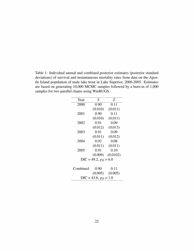
Table 1: Individual annual and combined posterior estimates (posterior standarddeviations) of survival and instantaneous mortality rates from data on the Apos-tle Island population of male lake trout in Lake Superior, 2000-2005. Estimatesare based on generating 10,000 MCMC samples followed by a burn-in of 1,000samples for two parallel chains using WinBUGS.

Year S Z2000 0.90 0.11

(0.010) (0.011)2001 0.90 0.11

(0.010) (0.011)2002 0.91 0.09

(0.012) (0.013)2003 0.91 0.09

(0.011) (0.012)2004 0.92 0.08

(0.011) (0.011)2005 0.91 0.10

(0.009) (0.0102)DIC = 49.2, pD = 6.0

Combined 0.90 0.11(0.005) (0.005)

DIC = 43.6, pD = 1.0

22

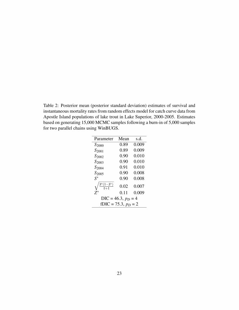
Table 2: Posterior mean (posterior standard deviation) estimates of survival andinstantaneous mortality rates from random effects model for catch curve data fromApostle Island populations of lake trout in Lake Superior, 2000-2005. Estimatesbased on generating 15,000 MCMC samples following a burn-in of 5,000 samplesfor two parallel chains using WinBUGS.

Parameter Mean s.d.S2000 0.89 0.009S2001 0.89 0.009S2002 0.90 0.010S2003 0.90 0.010S2004 0.91 0.010S2005 0.90 0.008S∗ 0.90 0.008√

S∗(1−S∗)τ+1 0.02 0.007

Z∗ 0.11 0.009DIC = 46.3, pD = 4fDIC = 75.3, pD = 2

23

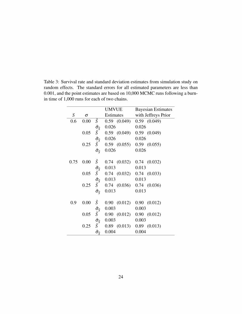
Table 3: Survival rate and standard deviation estimates from simulation study onrandom effects. The standard errors for all estimated parameters are less than0.001, and the point estimates are based on 10,000 MCMC runs following a burn-in time of 1,000 runs for each of two chains.

UMVUE Bayesian EstimatesS σ Estimates with Jeffreys Prior

0.6 0.00 S 0.59 (0.049) 0.59 (0.049)σS 0.026 0.026

0.05 S 0.59 (0.049) 0.59 (0.049)σS 0.026 0.026

0.25 S 0.59 (0.055) 0.59 (0.055)σS 0.026 0.026

0.75 0.00 S 0.74 (0.032) 0.74 (0.032)σS 0.013 0.013

0.05 S 0.74 (0.032) 0.74 (0.033)σS 0.013 0.013

0.25 S 0.74 (0.036) 0.74 (0.036)σS 0.013 0.013

0.9 0.00 S 0.90 (0.012) 0.90 (0.012)σS 0.003 0.003

0.05 S 0.90 (0.012) 0.90 (0.012)σS 0.003 0.003

0.25 S 0.89 (0.013) 0.89 (0.013)σS 0.004 0.004

24

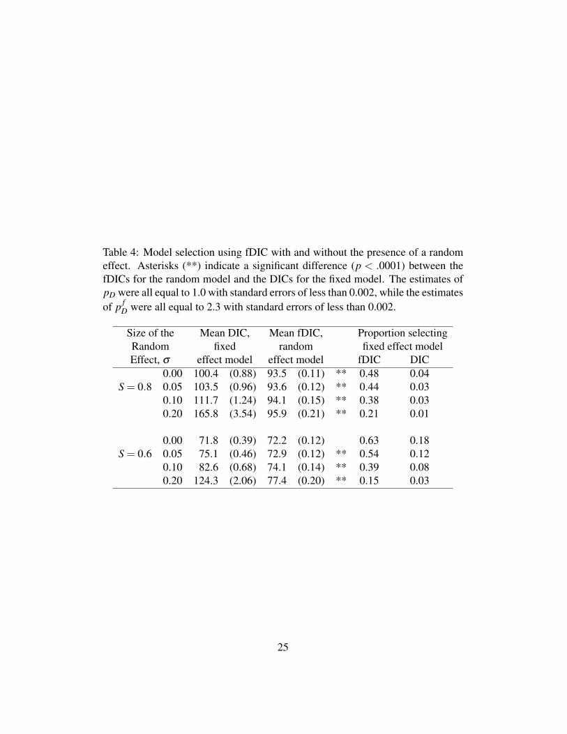
Table 4: Model selection using fDIC with and without the presence of a randomeffect. Asterisks (**) indicate a significant difference (p < .0001) between thefDICs for the random model and the DICs for the fixed model. The estimates ofpD were all equal to 1.0 with standard errors of less than 0.002, while the estimatesof p f

D were all equal to 2.3 with standard errors of less than 0.002.

Size of the Mean DIC, Mean fDIC, Proportion selectingRandom fixed random fixed effect modelEffect, σ effect model effect model fDIC DIC

0.00 100.4 (0.88) 93.5 (0.11) ** 0.48 0.04S = 0.8 0.05 103.5 (0.96) 93.6 (0.12) ** 0.44 0.03

0.10 111.7 (1.24) 94.1 (0.15) ** 0.38 0.030.20 165.8 (3.54) 95.9 (0.21) ** 0.21 0.01

0.00 71.8 (0.39) 72.2 (0.12) 0.63 0.18S = 0.6 0.05 75.1 (0.46) 72.9 (0.12) ** 0.54 0.12

0.10 82.6 (0.68) 74.1 (0.14) ** 0.39 0.080.20 124.3 (2.06) 77.4 (0.20) ** 0.15 0.03

25