IDA Document NS D-5831

July 2016

Bayesian Analysis in R/STAN

Kassandra Fronczyk

Log: H 16-000723

I N S T I T U T E F O R D E F E N S E A N A L Y S E S

INSTITUTE FOR DEFENSE ANALYSES4850 Mark Center Drive

Alexandria, Virginia 22311-1882

Approved for public release.

The Institute for Defense Analyses is a non-profit corporation that operates three federally funded research and development centers to provide objective analyses of national security issues, particularly those requiring scientific and technical expertise, and conduct related research on other national challenges.

About This PublicationIn an era of reduced budgets and limited testing, verifying that requirements have been met in a single test period can be challenging, particularly using traditional analysis methods that ignore all available information. The Bayesian paradigm is tailor made for these situations, allowing for the combination of multiple sources of data and resulting in more robust inference and uncertainty quantification. Consequently, Bayesian analyses are becoming increasingly popular in T&E. This tutorial briefly introduces the basic concepts of Bayesian Statistics, with implementation details illustrated in R through two case studies: reliability for the Core Mission functional area of the Littoral Combat Ship (LCS) and performance curves for a chemical detector in the Bio-chemical Detection System (BDS) with different agents and matrices. Examples are also presented using STAN, a high-performance open-source software for Bayesian inference on multi-level models.

Copyright Notice© 2016 Institute for Defense Analyses4850 Mark Center Drive, Alexandria, Virginia 22311-1882 • (703) 845-2000.

This material may be reproduced by or for the U.S. Government pursuant to the copyright license under the clause at DFARS 252.227-7013 (a)(16) [Jun 2013].

Bayesian Analysis in R/STAN

Kassandra Fronczyk

I N S T I T U T E F O R D E F E N S E A N A L Y S E S

IDA Document NS D-5831

i

Executive Summary

In an era of reduced budgets and limited testing, verifying that requirements have been met in a single test period can be challenging, particularly using traditional analysis methods that ignore all available information. The Bayesian paradigm is tailor made for these situations, allowing for the combination of multiple sources of data and resulting in more robust inference and uncertainty quantification. This tutorial is meant to introduce the basic concepts of Bayesian analysis. Further illustration of the flexibility and applicability of these methods is shown with examples from the T&E community, including implementation details. The course consists of four sections:

Fundamentals of Bayesian Analysis: This section provides the basic concepts common to all Bayesian analyses, including the specifications of prior distributions, likelihood functions, and posterior distributions. A simple example is used for demonstrative purposes, including a short sensitivity study.

Case study: Littoral Combat Ship (LCS). This section extends the simple component/subsystem level analysis shown in the first section and extends it to a

system reliability calculation. Here, LCS has a functional area reliability requirement, but data were collected on various subsystems of different data types. Implementation details are given in code snippets.

Case Study: Bio-chemical Detection System (BDS). This example takes the simple modeling case from the introduction and introduces factors of interest. A logistic regression model is fit to determine the probability of detection across different concentration levels of various chemical or biological agent/matrix concentrations. Implementation details are provided, along with a list of R packages that can aid in the fitting of these types of models.

8/1/2016-1

Bayesian Data Analysis in R/STAN

Dr. Kassie FronczykInstitute for Defense Analyses

Dr. James BrownlowUS Air Force

8/1/2016-2

Outline

• Fundamentals of Bayesian Analysis

• Case study: Littoral Combat Ship (LCS)

• Case Study: Bio-chemical Detection System (BDS)

• STAN Examples

8/1/2016-3

Acceptance of Bayesian Techniques

Bayesian methods are commonly used and becoming more widely accepted

• Applications– FAA/USAF in estimating probability of success of launch vehicles– Delphi Automotive for new fuel injection systems– Science-based Stockpile Stewardship program at LANL for

nuclear warheads– Army for estimating reliability of new aircraft systems– FDA for approving new medical devices

• Recent High Profile Successes:– During the search for Air France 447 (2009-2011), black box

location– The Coast Guard in 2013 found the missing fisherman, John

Aldridge

8/1/2016-4

Classical versus Bayesian Statistics

• Experiment 1: – A fine musician, specializing

in classical works, tells us that he is able to distinguish if Haydn or Mozart composed some classical song. Small excerpts of the compositions of both authors are selected at random and the experiment consists of playing them for identification by the musician. The musician makes 10 correct guesses in 10 trials.

• Experiment 2: – The guy next to you at the bar

says he can correctly guess in a coin toss what face of the coin will fall down. Again, after 10 trials the man correctly guesses the outcomes of the 10 throws.

8/1/2016-5

Classical versus Bayesian Statistics

• Classical Statistics Analysis– You have the same

confidence in the musician’s ability to identify composers as in the bar guy’s ability to predict coin tosses. In both cases, there were 10 successes in 10 trials.

• Bayesian Statistics Analysis – Presumably, you are

inclined to have more confidence in the musician’s claim than the guy at the bar’s claim. Post analysis, the credibility of both claims will have increased, though the musician will continue to have more credibility than bar guy.

8/1/2016-6

Bayesian Statistics 101

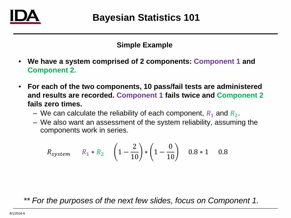
Simple Example

• We have a system comprised of 2 components: Component 1 and Component 2.

• For each of the two components, 10 pass/fail tests are administered and results are recorded. Component 1 fails twice and Component 2fails zero times.

– We can calculate the reliability of each component, 𝑅𝑅1 and 𝑅𝑅2.– We also want an assessment of the system reliability, assuming the

components work in series.

𝑅𝑅𝑠𝑠𝑠𝑠𝑠𝑠𝑠𝑠𝑠𝑠𝑠𝑠 = 𝑅𝑅1 ∗ 𝑅𝑅2 = 1 −2

10 ∗ 1 −0

10 = 0.8 ∗ 1 = 0.8

** For the purposes of the next few slides, focus on Component 1.

8/1/2016-7

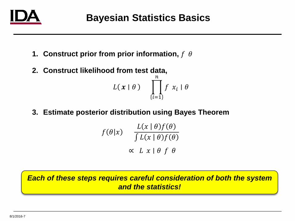
Bayesian Statistics Basics

1. Construct prior from prior information, 𝑓𝑓(𝜃𝜃)

2. Construct likelihood from test data,

𝐿𝐿 𝒙𝒙 𝜃𝜃 = �𝑖𝑖=1

𝑛𝑛

𝑓𝑓(𝑥𝑥𝑖𝑖 ∣ 𝜃𝜃)

3. Estimate posterior distribution using Bayes Theorem

Each of these steps requires careful consideration of both the system and the statistics!

𝑓𝑓 𝜃𝜃 𝑥𝑥 =𝐿𝐿 𝑥𝑥 𝜃𝜃 𝑓𝑓 𝜃𝜃∫ 𝐿𝐿 𝑥𝑥 𝜃𝜃 𝑓𝑓 𝜃𝜃

∝ 𝐿𝐿(𝑥𝑥 ∣ 𝜃𝜃)𝑓𝑓(𝜃𝜃)

8/1/2016-8

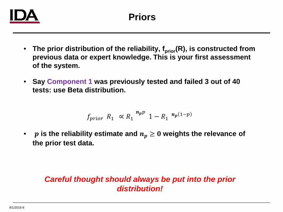
Priors

• The prior distribution of the reliability, fprior(R), is constructed from previous data or expert knowledge. This is your first assessment of the system.

• Say Component 1 was previously tested and failed 3 out of 40 tests: use Beta distribution.

𝑓𝑓𝑝𝑝𝑝𝑝𝑖𝑖𝑝𝑝𝑝𝑝(𝑅𝑅1) ∝ 𝑅𝑅1𝒏𝒏𝒑𝒑𝑝𝑝(1 − 𝑅𝑅1)𝒏𝒏𝒑𝒑 1−𝑝𝑝

• 𝒑𝒑 is the reliability estimate and 𝒏𝒏𝒑𝒑 ≥ 𝟎𝟎 weights the relevance of the prior test data.

Careful thought should always be put into the prior distribution!

8/1/2016-9

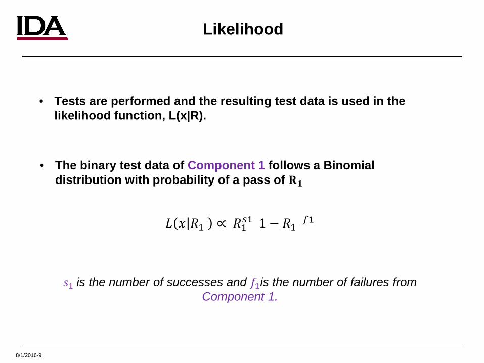
Likelihood

• Tests are performed and the resulting test data is used in the likelihood function, L(x|R).

• The binary test data of Component 1 follows a Binomial distribution with probability of a pass of 𝐑𝐑𝟏𝟏

𝐿𝐿 𝑥𝑥 𝑅𝑅1 ∝ 𝑅𝑅1𝑠𝑠1(1 − 𝑅𝑅1)𝑓𝑓1

𝑠𝑠1 is the number of successes and 𝑓𝑓1is the number of failures from Component 1.

8/1/2016-10

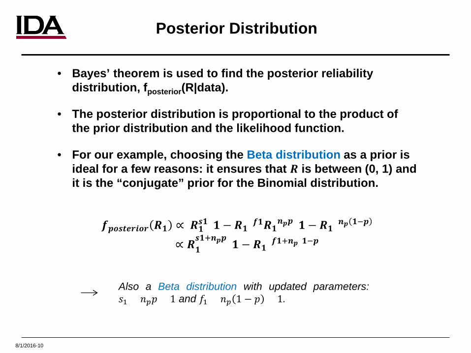
Posterior Distribution

• Bayes’ theorem is used to find the posterior reliability distribution, fposterior(R|data).

• The posterior distribution is proportional to the product of the prior distribution and the likelihood function.

• For our example, choosing the Beta distribution as a prior is ideal for a few reasons: it ensures that 𝑹𝑹 is between (0, 1) and it is the “conjugate” prior for the Binomial distribution.

𝒇𝒇𝒑𝒑𝒑𝒑𝒑𝒑𝒑𝒑𝒑𝒑𝒑𝒑𝒑𝒑𝒑𝒑𝒑𝒑 𝑹𝑹𝟏𝟏 ∝ 𝑹𝑹𝟏𝟏𝒑𝒑𝟏𝟏(𝟏𝟏 − 𝑹𝑹𝟏𝟏)𝒇𝒇𝟏𝟏𝑹𝑹𝟏𝟏𝒏𝒏𝒑𝒑𝒑𝒑(𝟏𝟏 − 𝑹𝑹𝟏𝟏)𝒏𝒏𝒑𝒑 𝟏𝟏−𝒑𝒑

∝ 𝑹𝑹𝟏𝟏𝒑𝒑𝟏𝟏+𝒏𝒏𝒑𝒑𝒑𝒑(𝟏𝟏 − 𝑹𝑹𝟏𝟏)𝒇𝒇𝟏𝟏+𝒏𝒏𝒑𝒑(𝟏𝟏−𝒑𝒑)

Also a Beta distribution with updated parameters:𝑠𝑠1 + 𝑛𝑛𝑝𝑝𝑝𝑝 + 1 and 𝑓𝑓1 + 𝑛𝑛𝑝𝑝 1 − 𝑝𝑝 + 1.

8/1/2016-11

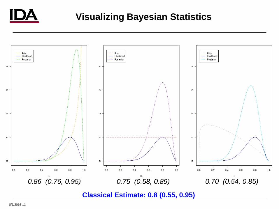
Visualizing Bayesian Statistics

0.86 (0.76, 0.95) 0.75 (0.58, 0.89) 0.70 (0.54, 0.85)

Classical Estimate: 0.8 (0.55, 0.95)

8/1/2016-12

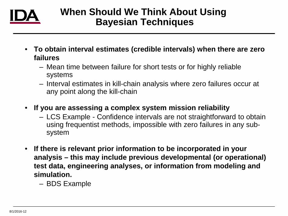
When Should We Think About Using Bayesian Techniques

• To obtain interval estimates (credible intervals) when there are zero failures

– Mean time between failure for short tests or for highly reliable systems

– Interval estimates in kill-chain analysis where zero failures occur at any point along the kill-chain

• If you are assessing a complex system mission reliability– LCS Example - Confidence intervals are not straightforward to obtain

using frequentist methods, impossible with zero failures in any sub-system

• If there is relevant prior information to be incorporated in your analysis – this may include previous developmental (or operational) test data, engineering analyses, or information from modeling and simulation.

– BDS Example

8/1/2016-13

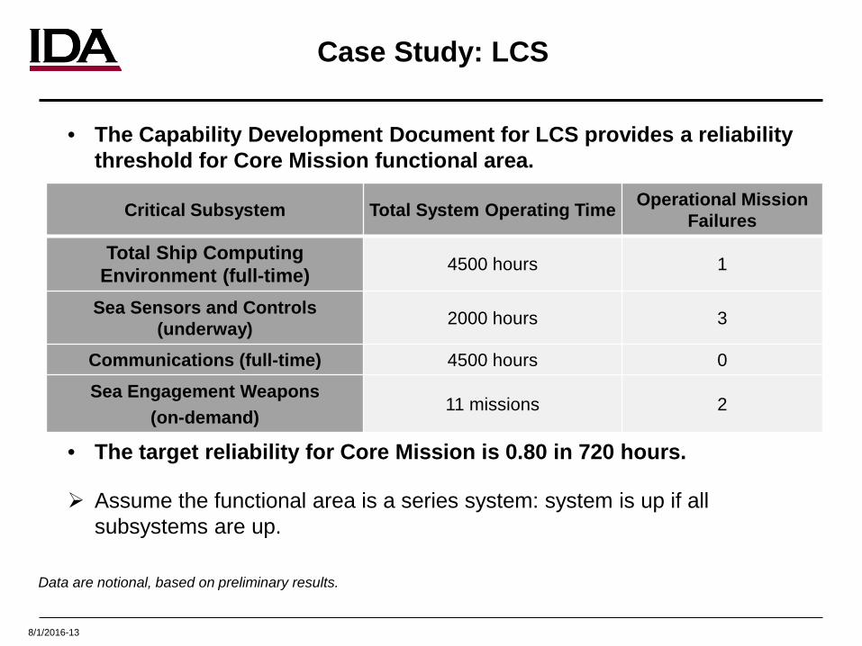
Case Study: LCS

• The Capability Development Document for LCS provides a reliability threshold for Core Mission functional area.

• The target reliability for Core Mission is 0.80 in 720 hours.

Assume the functional area is a series system: system is up if all subsystems are up.

Critical Subsystem Total System Operating Time Operational Mission Failures

Total Ship Computing Environment (full-time) 4500 hours 1

Sea Sensors and Controls (underway) 2000 hours 3

Communications (full-time) 4500 hours 0

Sea Engagement Weapons (on-demand)

11 missions 2

Data are notional, based on preliminary results.

8/1/2016-14

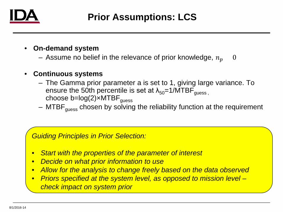
Prior Assumptions: LCS

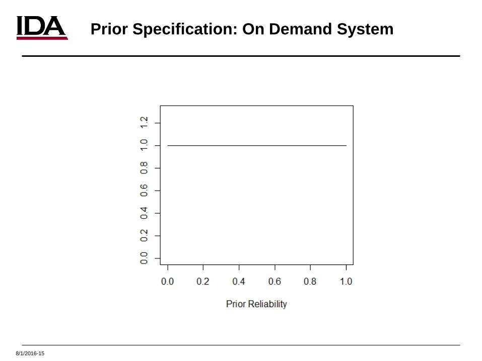
• On-demand system– Assume no belief in the relevance of prior knowledge, 𝑛𝑛𝑝𝑝 = 0

• Continuous systems– The Gamma prior parameter a is set to 1, giving large variance. To

ensure the 50th percentile is set at λ50=1/MTBFguess ,choose b=log(2)×MTBFguess

– MTBFguess chosen by solving the reliability function at the requirement

Guiding Principles in Prior Selection:

• Start with the properties of the parameter of interest• Decide on what prior information to use• Allow for the analysis to change freely based on the data observed• Priors specified at the system level, as opposed to mission level –

check impact on system prior

8/1/2016-15

Prior Specification: On Demand System

8/1/2016-16

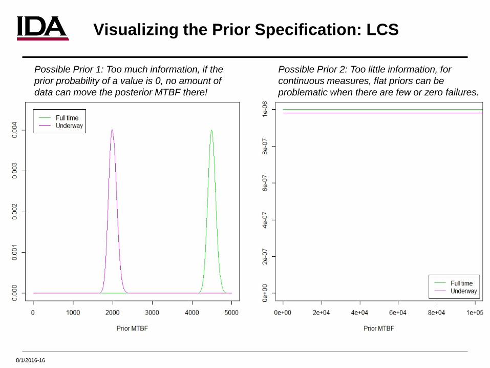
Visualizing the Prior Specification: LCS

Possible Prior 1: Too much information, if the prior probability of a value is 0, no amount of data can move the posterior MTBF there!

Possible Prior 2: Too little information, for continuous measures, flat priors can be problematic when there are few or zero failures.

8/1/2016-17

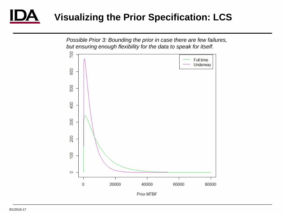
Visualizing the Prior Specification: LCS

Possible Prior 3: Bounding the prior in case there are few failures, but ensuring enough flexibility for the data to speak for itself.

8/1/2016-18

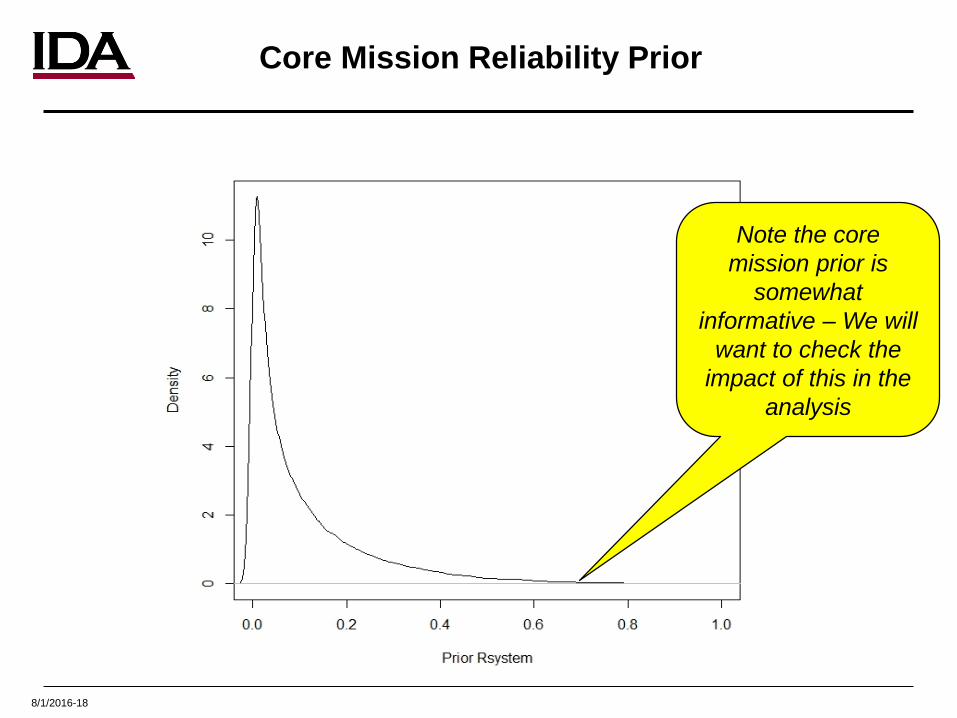
Core Mission Reliability Prior

Note the core mission prior is

somewhat informative – We will

want to check the impact of this in the

analysis

8/1/2016-19

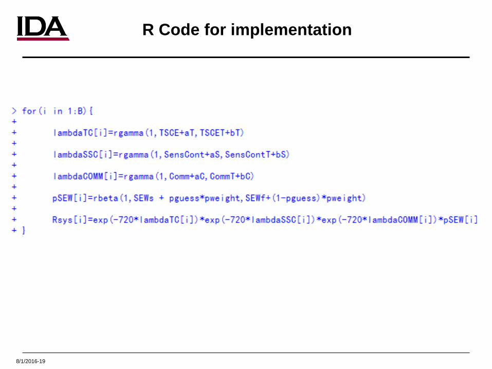
R Code for implementation

8/1/2016-20

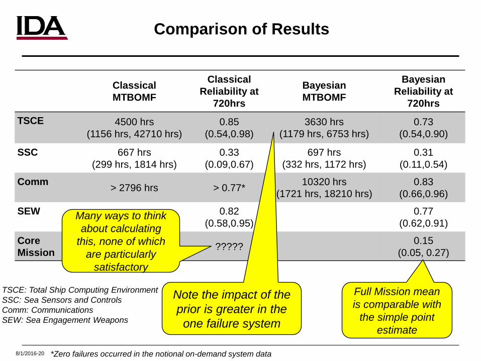
Comparison of Results

ClassicalMTBOMF

ClassicalReliability at

720hrs

BayesianMTBOMF

BayesianReliability at

720hrsTSCE 4500 hrs

(1156 hrs, 42710 hrs)0.85

(0.54,0.98)3630 hrs

(1179 hrs, 6753 hrs)0.73

(0.54,0.90)

SSC 667 hrs(299 hrs, 1814 hrs)

0.33(0.09,0.67)

697 hrs(332 hrs, 1172 hrs)

0.31 (0.11,0.54)

Comm > 2796 hrs > 0.77* 10320 hrs(1721 hrs, 18210 hrs)

0.83 (0.66,0.96)

SEW 0.82(0.58,0.95)

0.77(0.62,0.91)

CoreMission ????? 0.15

(0.05, 0.27)

*Zero failures occurred in the notional on-demand system data

Note the impact of the prior is greater in the one failure system

Full Mission mean is comparable with

the simple point estimate

TSCE: Total Ship Computing EnvironmentSSC: Sea Sensors and ControlsComm: CommunicationsSEW: Sea Engagement Weapons

Many ways to think about calculating

this, none of which are particularly

satisfactory

8/1/2016-21

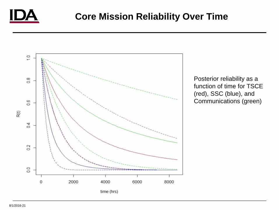
Core Mission Reliability Over Time

Posterior reliability as a function of time for TSCE (red), SSC (blue), and Communications (green)

8/1/2016-22

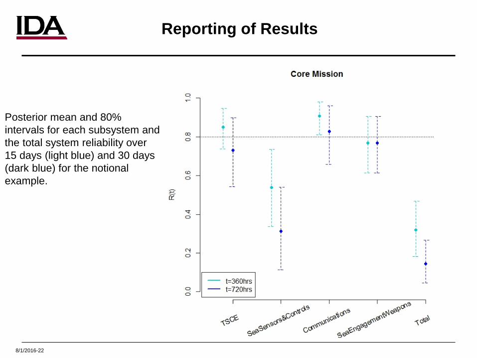
Reporting of Results

Posterior mean and 80% intervals for each subsystem and the total system reliability over 15 days (light blue) and 30 days (dark blue) for the notional example.

8/1/2016-23

Value of Bayesian Statistics for LCS

• Avoids unrealistic reliability estimates when there are no observed failures.

• In our notional example (zero failures for the Communications system), the Bayesian approach helped us solve an otherwise intractable problem.

• Obtaining interval estimates is straightforward for system reliability

– Frequentist methods would have to employ the Delta method, Normal approximations, or bootstrapping.

• Flexibility in developing system models– We used a series system for the core mission reliability– Many other system models are possible and we can still get

full system reliability estimates with intervals.

8/1/2016-24

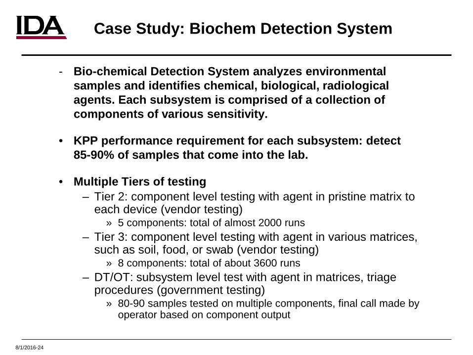
Case Study: Biochem Detection System

- Bio-chemical Detection System analyzes environmental samples and identifies chemical, biological, radiological agents. Each subsystem is comprised of a collection of components of various sensitivity.

• KPP performance requirement for each subsystem: detect 85-90% of samples that come into the lab.

• Multiple Tiers of testing– Tier 2: component level testing with agent in pristine matrix to

each device (vendor testing)» 5 components: total of almost 2000 runs

– Tier 3: component level testing with agent in various matrices, such as soil, food, or swab (vendor testing)

» 8 components: total of about 3600 runs– DT/OT: subsystem level test with agent in matrices, triage

procedures (government testing)» 80-90 samples tested on multiple components, final call made by

operator based on component output

8/1/2016-25

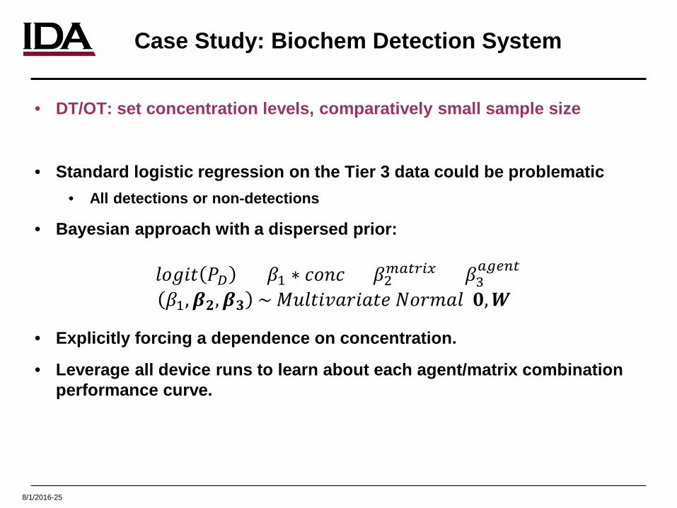
• DT/OT: set concentration levels, comparatively small sample size

• Standard logistic regression on the Tier 3 data could be problematic• All detections or non-detections

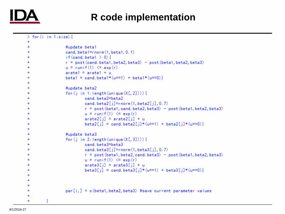
• Bayesian approach with a dispersed prior:

𝑙𝑙𝑙𝑙𝑙𝑙𝑙𝑙𝑙𝑙 𝑃𝑃𝐷𝐷 = 𝛽𝛽1 ∗ 𝑐𝑐𝑙𝑙𝑛𝑛𝑐𝑐 + 𝛽𝛽2𝑠𝑠𝑚𝑚𝑠𝑠𝑝𝑝𝑖𝑖𝑚𝑚 + 𝛽𝛽3𝑚𝑚𝑎𝑎𝑠𝑠𝑛𝑛𝑠𝑠

𝛽𝛽1,𝜷𝜷𝟐𝟐,𝜷𝜷𝟑𝟑 ~ 𝑀𝑀𝑀𝑀𝑙𝑙𝑙𝑙𝑙𝑙𝑀𝑀𝑀𝑀𝑀𝑀𝑙𝑙𝑀𝑀𝑙𝑙𝑀𝑀 𝑁𝑁𝑙𝑙𝑀𝑀𝑁𝑁𝑀𝑀𝑙𝑙(𝟎𝟎,𝑾𝑾)

• Explicitly forcing a dependence on concentration.

• Leverage all device runs to learn about each agent/matrix combination performance curve.

Case Study: Biochem Detection System

8/1/2016-26

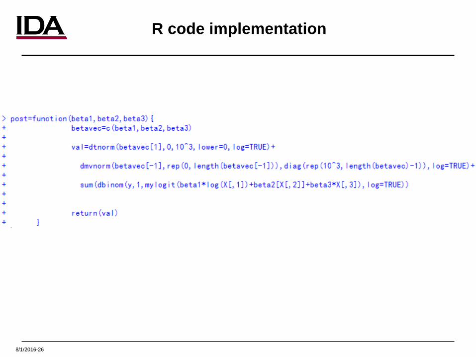
R code implementation

8/1/2016-27

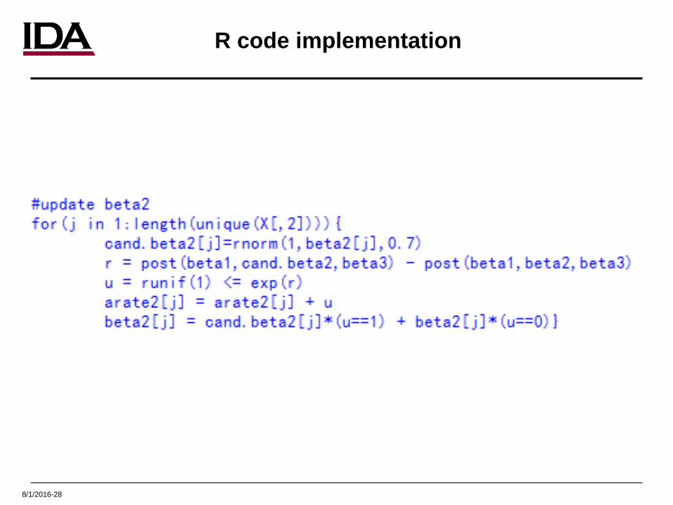
R code implementation

8/1/2016-28

R code implementation

8/1/2016-29

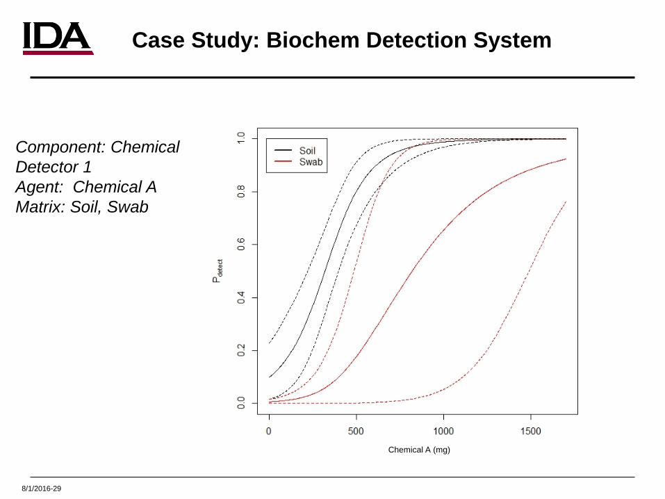
Component: Chemical Detector 1Agent: Chemical AMatrix: Soil, Swab

Chemical A (mg)

Case Study: Biochem Detection System

8/1/2016-30

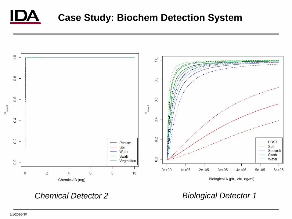
Chemical Detector 2 Biological Detector 1

Chemical B (mg) Biological A (pfu, cfu, ng/ml)

Case Study: Biochem Detection System

8/1/2016-31

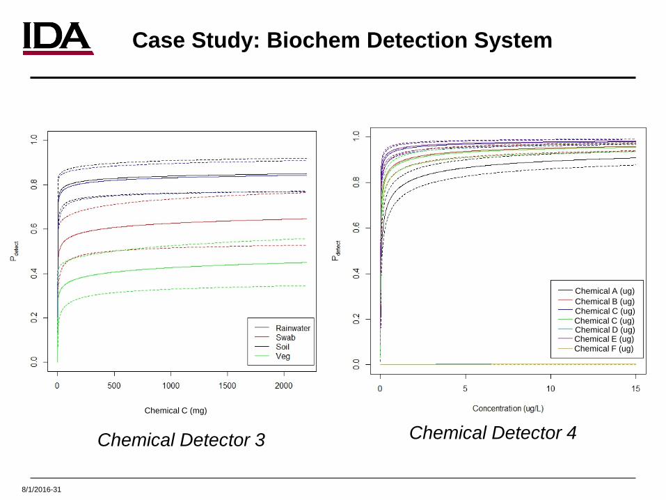
Chemical Detector 3 Chemical Detector 4Chemical C (mg)

Chemical A (ug)Chemical B (ug)Chemical C (ug)Chemical C (ug)Chemical D (ug)Chemical E (ug)Chemical F (ug)

Case Study: Biochem Detection System

8/1/2016-32

Value of Bayesian Statistics for Biochem Detection System

• Tier 2 and Tier 3 produced a lot of data which we can leverage to make informed decisions.

• By knowing the concentrations of agents within various matrices that each component can detect, we can determine concentrations that the system of devices might be easy or difficult for the operators to identify in DT/OT.

• This analysis can serve as the basis for the analysis of the DT/OT data.

8/1/2016-33

Discussion: When Is it Worth the Effort?

• Inclusion of prior information from prior testing, modeling and simulation, or engineering analyses only when it is relevant to the current test. We do not want to bias the OT results.

• Even when including prior information, the prior must have enough variability to allow the estimates to move away from what was previously seen if the data support such values.

• We can use very flexible models for many types of test data (e.g. kill chains, complex system structures, linking EFFs to SA) and obtain estimates more readily than with the frequentist paradigm. The model and assumptions have to make sense for the test at hand.

8/1/2016-34

Discussion: Other Resources

• For other R packages that provide easy to implement tools and short but informative how to guides with examples, see

https://cran.r-project.org/web/views/Bayesian.html

arm, bayesm, and bayesSurv are good places to start

As with any new statistical method, it is important to have an expert review your work the first few times you apply these

techniques. There are many ways to accidentally do bad statistics!

8/1/2016-35

Backup Slides

8/1/2016-36

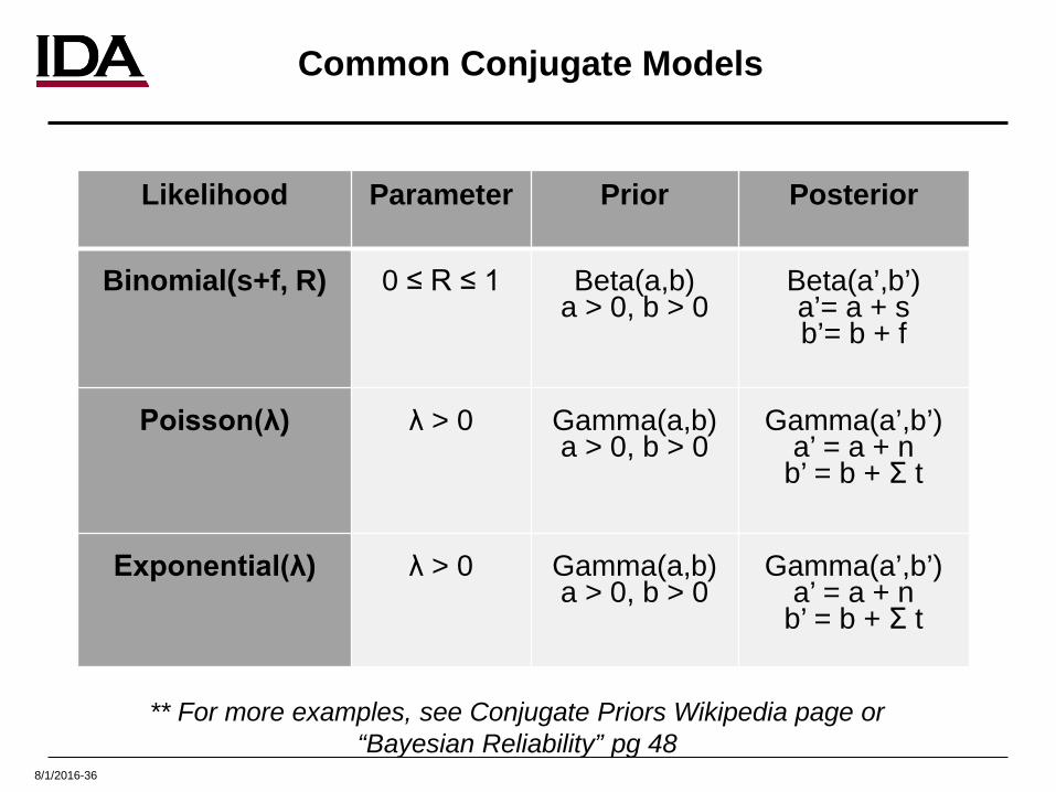
Common Conjugate Models

Likelihood Parameter Prior Posterior

Binomial(s+f, R) 0 ≤ R ≤ 1 Beta(a,b)a > 0, b > 0

Beta(a’,b’)a’= a + sb’= b + f

Poisson(λ) λ > 0 Gamma(a,b)a > 0, b > 0

Gamma(a’,b’) a’ = a + n

b’ = b + Σ t

Exponential(λ) λ > 0 Gamma(a,b)a > 0, b > 0

Gamma(a’,b’) a’ = a + n

b’ = b + Σ t

** For more examples, see Conjugate Priors Wikipedia page or “Bayesian Reliability” pg 48