Embed Size (px)
Citation preview
Batteries and Battery Management:
Development of Low Cost,
Rapid Impedance Measurement
Equipment Suitable for Fast Analysis
of Li-ion Cells
Huw Price
MPhil Thesis
October 2014
110109181
Supervisor: Prof. D.A. Stone
Second Supervisor: Dr M.P. Foster

1
ABSTRACT - Batteries are a vital and integral part of modern life, installed in devices of
every scale from personal portable electronic equipment to electricity grid energy storage.
As people become increasingly dependent on battery energy sources, they also become
increasingly reliant on accurate methods of quantifying the amount of useful energy available
to them in order to function in their daily lives. Electrochemical Impedance Spectroscopy
(EIS) is a branch of System Identification that can be used to identify battery metrics by
which the remaining short-term (i.e. remaining charge) and long-term (battery lifetime
remaining) life of a battery may be assessed. In this thesis the author gives an overview of
battery chemistries and battery state estimation techniques before describing the development
of a system capable of performing rapid impedance measurements. The development process
spans two system designs, and results are given of impedance tests on lithium iron phosphate
cells (LiFePO4) and lithium titanate (Li4Ti5O12) cells. A key feature of the method is to use
Pseudo-Random Binary Sequences (PRBS) to approximate white noise, thereby providing
equal stimulation of a wide band of frequencies simultaneously and reducing the required
test-time. This document will be of use to those wishing to develop EIS test equipment at
low-cost, and those who require a method of rapidly obtaining an impedance spectrum.

2
This work was supported by the Engineering and Physical Sciences Research Council,
and I wish to thank Professor Dave Stone and Dr Martin Foster for the opportunity and
guidance.
I would also like to thank my peers from E125 - Dan Rogers, Dan Schofield, Chi Tsang
and Andrew Fairweather – for the friendship, inspiration and humour shown while
providing stimulating discussion. I am grateful to Dr James Green for his tireless support
since my undergraduate days, and to my colleague Jonathan Davidson for always being
willing to answer just one more question. Thanks are also due to Dr Anthony Rennie for
always being prepared to run just one more test.
I am grateful to Lawrence Obodo, Ian Lyne, Dick Savage, and John Wilkinson for their
practical support and guidance, always in good faith and humour. Emma Foster provided
mentor support and friendship which was instrumental to the completion of the work. Over
the years I have made many friends in Sheffield who are too many to name but have all
contributed to my time here in countless ways – you know who you are, and thank you.
Several times I came close to walking away and without you this page would not exist.
I am indebted to my ex-wife Maia Hunnex, without whom I would not have had the
opportunity to do any post-graduate research and who suffered the most in the early days – I
wish I could say it was worth it. I am grateful to Yasmin Badat for her love, support and
friendship over the last year.
Finally to my family – Peter, Twiggy, Inga and Pete, Pip, Michael, Sean and Keira – who
have patiently and relentlessly supported me throughout; I am looking forward to seeing a
lot more of you all. Thank you.
3
Contents
List of Figures .........................................................................................................................5
List of Tables ..........................................................................................................................7
List of Acronyms ....................................................................................................................8
Chapter 1: Introduction .....................................................................................................10
1.1 A Background to Battery Technologies .................................................................10
1.1.1 Lead Acid (Pb-acid) Batteries .........................................................................10
1.1.2 Nickel Cadmium (Ni-Cd) and Nickel-Metal Hydride (Ni-MH) Batteries ......12
1.1.3 Lithium-Ion Batteries ......................................................................................13
1.2 Battery Management Systems (BMS) ....................................................................16
1.2.1 Function of the BMS .......................................................................................17
1.2.2 Key Estimation Metrics ..................................................................................18
1.2.3 Battery State Estimation Tools .......................................................................21
1.3 Electrochemical Impedance Spectroscopy (EIS) ...................................................28
1.3.1 The Relationship between Battery Impedance and Battery Dynamics ...........28
1.3.2 Standard Laboratory EIS Techniques .............................................................30
1.3.3 Pseudo-Random Binary Sequences (PRBS) as Pseudo-White Noise Input ...31
1.4 Conclusions ............................................................................................................34
Chapter 2: Battery Charge Cycler and PRBS Impedance Measurement Rig ...................35
2.1 Objectives ...............................................................................................................35
2.2 High Current Cycling Rig ......................................................................................36
2.3 PRBS Impedance Test Rig .....................................................................................37
Contents
4
2.4 Test Procedure ....................................................................................................... 40
2.5 Impedance Tests .................................................................................................... 41
2.5.1 Stimulus Signals ............................................................................................. 41
2.5.2 Post-Processing .............................................................................................. 41
2.6 Results ................................................................................................................... 42
2.6.1 26650E LiFePO4 (LFP) Cells ........................................................................ 43
2.6.2 LTO Polymer (Pouch) SLPB Cells ................................................................ 53
2.7 Preliminary Findings and Suggested Changes ...................................................... 58
2.7.1 Charge Cycling............................................................................................... 58
2.7.2 PRBS Impedance Testing .............................................................................. 58
Chapter 3: Charge Cycler/Impedance Analyser Specification and Design ..................... 60
3.1 Objectives .............................................................................................................. 60
3.2 Hardware Design and Construction ...................................................................... 60
3.2.1 Target Specification ....................................................................................... 60
3.2.2 Design Steps ................................................................................................... 61
3.3 Theoretical Limits ................................................................................................. 69
3.4 Control Software ................................................................................................... 70
3.4.1 User Interface and Test Options ..................................................................... 70
3.4.2 PRBS Post-Processing ................................................................................... 75
3.5 Hardware Performance Characteristics ................................................................. 76
3.5.1 Charge Cycling and Pulsed Discharge ........................................................... 76
3.5.2 PRBS – Time Domain Signals ....................................................................... 78
3.5.3 PRBS – Frequency Response ......................................................................... 80
3.6 Example Results .................................................................................................... 83
List of Figures
5
3.7 Conclusion ..............................................................................................................84
Chapter 4: Conclusions and Suggestions for Further Work .............................................85
4.1.1 PRBS Impedance Testing ...............................................................................85
4.2 References ..............................................................................................................88
Appendix 1. ...........................................................................................................................92
List of Figures
Figure 1.1 – A 1 MW/1.4 MWh BESS at Metlakatla Power & Light, Alaska. The installation
consists of 378 Exide VRLA modules. .................................................................................11
Figure 1.2- NTSB photos of the burned auxiliary power unit battery from a JAL Boeing 787
that caught fire on Jan. 7 at Boston's Logan International Airport. ......................................16
Figure 1.3 - Charge and Discharge Curves for Various Lithium-ion Cell Chemistries........22
Figure 1.4 - An example of membership function for State of Health .................................26
Figure 1.5 – An overview of the Fuzzy Logic Process .........................................................26
Figure 1.6 – The major components of a Lithium-Ion Cell ..................................................28
Figure 1.7 – A typical Li-ion Nyquist impedance plot, showing identifiable characteristics of
dynamic mechanisms in a new cell .......................................................................................29
Figure 1.8 – 6-bit shift register showing the feedback tap connections used to produce a
maximum-length sequence (MLS)........................................................................................32
Figure 1.9 – A 1 Hz bipolar PRBS signal produced from a 6-bit shift register ....................32
Figure 1.10 – Normalised PSD of the PRBS signal seen in Figure 1.9 ................................33
Figure 2.1 - Control Board and Single Output (One of Four), ..............................................36
Figure 2.2 – PRBS load control ............................................................................................38
Figure 2.3 – Cycling Rig and PRBS Impedance Tester ........................................................39
Figure 2.4 – Standard Discharge Voltage Characteristic ......................................................44
List of Figures
6
Figure 2.5 - Standard Recharge Characteristic .................................................................... 44
Figure 2.6 – Measured Cell Capacities ................................................................................ 45
Figure 2.7 - Cell OCV, SoC and Temperature ..................................................................... 46
Figure 2.8 – Impedance, SoC, and Temperature .................................................................. 48
Figure 2.9 – OCV vs Nominal SoC for New and Aged Cells.............................................. 49
Figure 2.10 – OCV vs Normalised SoC for New and Aged Cells ....................................... 49
Figure 2.11 – Impedance (0-0.5 Hz), SoC and Temperature for New and Aged Cells ....... 50
Figure 2.12 – Comparison of PRBS Impedance Results with EIS Swept Sine Results ...... 51
Figure 2.13 – PDC Voltage Curves: New and Aged LTO Cells ......................................... 53
Figure 2.14 – OCV vs Normalised SoC, New and Aged LTO Cells ................................... 54
Figure 2.15 – PRBS Impedance Test Results, New and Aged LTO Cells .......................... 55
Figure 2.16 – New LTO Cell Impedance Spectrum at 100 % SoC ..................................... 56
Figure 2.18 – New LTO Cell PRBS Current and Voltage Showing Poor Resolution ......... 57
Figure 2.17 – Aged LTO Cell PRBS Current and Voltage .................................................. 57
Figure 3.1 – TIP3055/2955 BJT Safe Operating Area, single device .................................. 62
Figure 3.2 – Output Stage Maximum Load ......................................................................... 63
Figure 3.3 – Heatsink Maximum Power Requirements ....................................................... 64
Figure 3.4 – Output Pre-Drivers and One Output Pair ........................................................ 65
Figure 3.5 – VAS with Current Source Load and Pre-Driver Bias ...................................... 66
Figure 3.6 - Differential Amplifier and Global Feedback.................................................... 67
Figure 3.7 – Simulated Open Loop Response ...................................................................... 68
Figure 3.8 – Test Rig Safe Operating Area .......................................................................... 70
Figure 3.9 – Virtual Instrument Controls Showing a Typical Test Sequence and Available
Test Options ......................................................................................................................... 71
Figure 3.10 – Charge and Discharge Settings ...................................................................... 72
List of Tables
7
Figure 3.11 – PRBS and Rest Time settings .........................................................................73
Figure 3.12 – Safety Limits and Acquisition Settings ..........................................................74
Figure 3.13 – Charge Cycling and Pulsed Discharge, 26650E Cell .....................................77
Figure 3.14 – Demonstration of 8 A amplitude PRBS .........................................................78
Figure 3.15 – Distortion as PRBS Clock (35 kHz) Approaches the Nyquist Limit (50 kHz)
...............................................................................................................................................79
Figure 3.16 – Nyquist Plot of Parallel RC Circuit Validation Test ......................................80
Figure 3.17 – Validation Test: Parallel RC Impedance plots, R = 1 Ω, C = 10 mF .............81
Figure 3.18 – Absolute Error between EIS and PRBS RC Impedance Data ........................82
Figure 3.19 – Impedance Data from a Large Capacity Cell .................................................83
Figure 3.20 – Nyquist Plot of Impedance, 50 Ah SLPB cell ................................................84
Figure A. 1 – 26650E Cell OCV vs SoC for each Cell Configuration .................................93
Figure A. 2 – 26650E Cells: OCV vs SoC at Fixed Temperatures, Comparing Cells .........94
Figure A. 3 – 26650E Cells: Average Impedance at 0-0.5 Hz vs SoC for each Cell
Configuration ........................................................................................................................95
Figure A. 4 - 26650E Cell Comparison at Fixed Temperature: Average Impedance at 0-
0.5 Hz vs SoC........................................................................................................................96
List of Tables
Table 2.1 – Chosen PRBS Clock Frequencies and Resultant Bandwidth of Spectrum ........41
Table 2.2 - Cell Reference Table ..........................................................................................43
Table 2.3 – Measured Capacity, New and Aged LTO Cells .................................................53
Table 3.1 – Minimum Requirements ....................................................................................61
Table 3.2 – Test Options .......................................................................................................74
8
Table 3.3 – Tested Specifications ........................................................................................ 76
List of Acronyms
ADC Analogue-to-Digital Converter
ANN Artificial Neural Network
BESS Battery Energy Storage System
BMS Battery Management System
C/LCO Graphite/Lithium Cobalt Oxide (LiCoO2)
C/LFP Graphite/Lithium Iron Phosphate (C/LiFePO4)
C/LMO Graphite/Lithium Manganese Oxide (C/LiMn2O4)
C/NCA Graphite/Lithium Nickel Cobalt Aluminium Oxide
(LiNiMnCoO2)
C/NCM Graphite/Lithium Nickel Manganese Cobalt Oxide
(LiNixMnyCozO2) (also C/NMC)
CAN Controller Area Network
DOD Depth of Discharge
DUT Device Under Test
EKF Extended Kalman Filter
EMF Electromotive Force
EOL End-Of-Life
FL Fuzzy Logic
FRF Frequency Response Function
HEV Hybrid Electric Vehicle
IC(E) Internal Combustion (Engine)
KF Kalman Filter
LTO Lithium Titanate anode material (Li4Ti5O12)
OBD On Board Diagnostics
OCV Open Circuit Voltage
PDC Pulsed Discharge
PRBS Pseudo-Random Binary Sequence
List of Acronyms
9
SEI Solid Electrolyte Interface
SLPB Super Lithium Polymer Battery
SOA Safe Operating Area
SoC State of Charge
SoF State of Function
SoH State of Health
VAS Voltage Amplification Stage
VRLA Valve-Regulated Lead-Acid, a type of Pb-acid Battery
10
Chapter 1: Introduction
The purpose of this chapter is to provide context for the author’s work. There is a brief
description of the most popular battery chemistries of the last two centuries, followed by a
more detailed look at Lithium-ion batteries and an outline of key current research in Battery
Management System (BMS) technology. This gives a platform from which the author’s
research into battery impedance testing using Pseudo-Random Binary Sequences (PRBS) can
be discussed.
1.1 A Background to Battery Technologies
1.1.1 Lead Acid (Pb-acid) Batteries
Lead-acid (Pb-acid) batteries are the most mature rechargeable battery technology, with over
150 years of development behind them. The batteries comprise of a series of cells containing
positive electrodes of lead dioxide and negative electrodes of sponge lead, which are
immersed in an aqueous sulphuric acid electrolyte and separated by a micro-porous material.
Broadly speaking, the batteries fall into two categories; the flooded (or ‘vented’) type, in
which the electrolyte is an aqueous sulphuric acid solution, or a valve-regulated (VRLA) type
in which the acid electrolyte is immobilized in a porous separator material, and a pressure
regulating valve seals the battery. The valve in VRLA batteries is a safety device and not an
operational mechanism.
Pb-acid batteries are low-cost, rugged and relatively tolerant to abuse [1]. They require
careful maintenance procedures to prevent large sulphate crystals from forming, which
reduce the overall battery capacity and can be difficult to break up during recharge. Crystal
formation is likely when the battery is over-discharged or kept in a discharged state [2].
Pb-acid battery technology is mature and widespread, the flooded cells being most commonly
used in Internal Combustion (IC) vehicles as starter batteries, and employed in fork lift trucks
and traditional ‘milk float’ vehicles. They are used in the leisure industry as off-grid power
for motor homes and marine craft, often coupled with diesel generators or charged from an
auxiliary drive. The largest configuration lead-acid batteries have been designed for bulk
energy storage, with disappointing results; in 1986 the Southern California Edison Chino
facility was commissioned to produce a 10 MW/40 MWh BESS (Battery Energy Storage
Introduction
11
System) plant which was the largest of its kind, but few people have promoted the technology
since as life-cycle costs are not competitive [3]. For applications with lower capacity
requirements, conventional batteries become more competitive as they are no longer
competing for the same market as the more typical bulk storage technologies such as
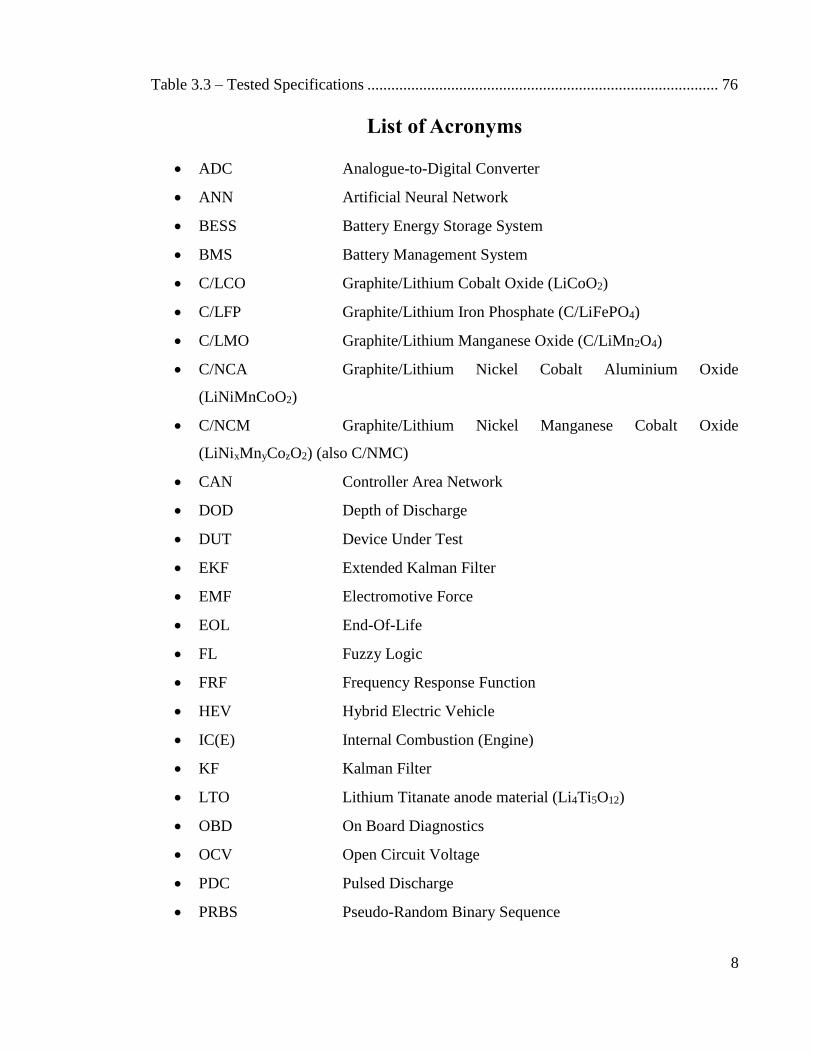
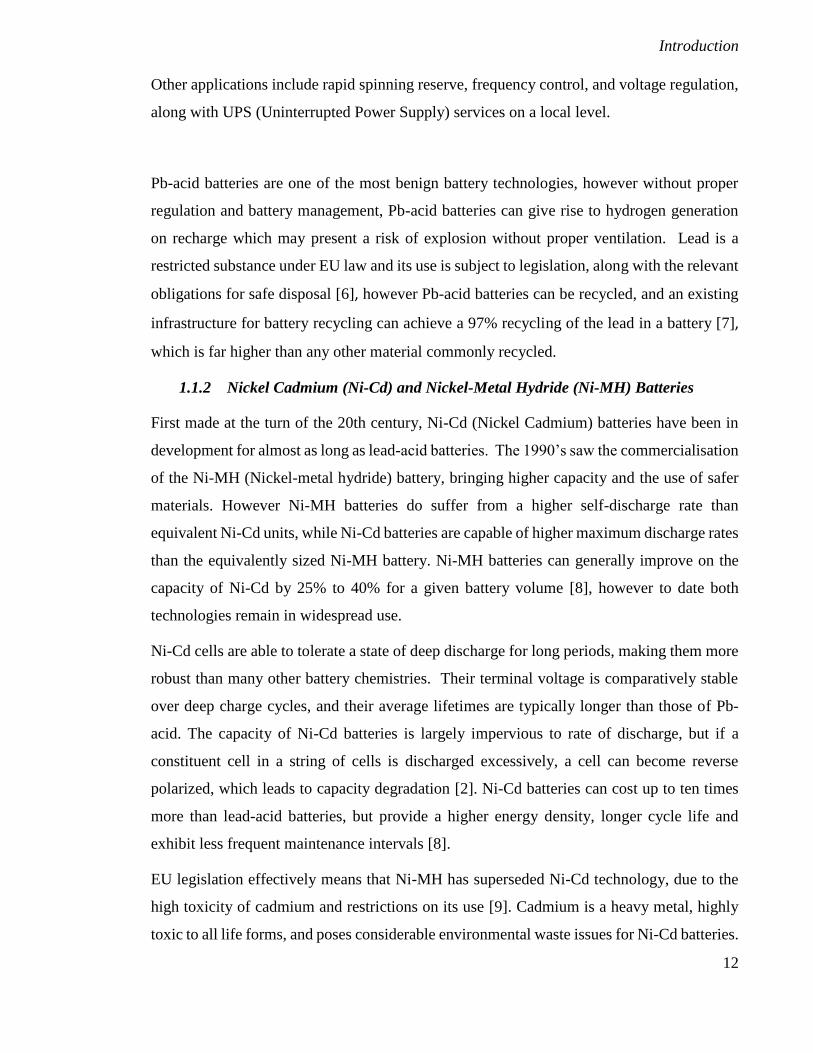
pumped-storage hydro-electric. Figure 1.1 shows a 1 MW/1.4 MWh installation at Metlakatla
Power & Light, Alaska, which is estimated to have saved over $6.5 Million over 12 years of
operation and exceeded initial life projection by almost 50 % [4]. A key factor to the success
of an installation such as this lies in the implementation of the Battery Management System
(BMS), which in this case maintained 378 VRLA batteries over a 12 year lifetime.
In 1994 a 21 MW / 14 MWh facility was installed at Sabana Llana by the Puerto Rico Electric
Power Authority (PREPA) to mitigate under-frequency load shedding, and whilst it was
operationally beneficial, it eventually failed prematurely and led to a governmental ‘lessons-
learned’ study in 1999 [5]. A major recommendation of this report is to invest considerable
resource in the accurate measurement and control of battery state-of-charge in any future
projects [5], as measurement of state of charge, and state of health is critical to obtaining the
best performance from any battery system, based on any chemistry.
Figure 1.1 – A 1 MW/1.4 MWh BESS at Metlakatla Power & Light, Alaska. The
installation consists of 378 Exide VRLA modules.
Source: DOE Global Energy Storage Database, www.energystorageexchange.org
Introduction
12
Other applications include rapid spinning reserve, frequency control, and voltage regulation,
along with UPS (Uninterrupted Power Supply) services on a local level.
Pb-acid batteries are one of the most benign battery technologies, however without proper
regulation and battery management, Pb-acid batteries can give rise to hydrogen generation
on recharge which may present a risk of explosion without proper ventilation. Lead is a
restricted substance under EU law and its use is subject to legislation, along with the relevant
obligations for safe disposal [6], however Pb-acid batteries can be recycled, and an existing
infrastructure for battery recycling can achieve a 97% recycling of the lead in a battery [7],
which is far higher than any other material commonly recycled.
1.1.2 Nickel Cadmium (Ni-Cd) and Nickel-Metal Hydride (Ni-MH) Batteries
First made at the turn of the 20th century, Ni-Cd (Nickel Cadmium) batteries have been in
development for almost as long as lead-acid batteries. The 1990’s saw the commercialisation
of the Ni-MH (Nickel-metal hydride) battery, bringing higher capacity and the use of safer
materials. However Ni-MH batteries do suffer from a higher self-discharge rate than
equivalent Ni-Cd units, while Ni-Cd batteries are capable of higher maximum discharge rates
than the equivalently sized Ni-MH battery. Ni-MH batteries can generally improve on the
capacity of Ni-Cd by 25% to 40% for a given battery volume [8], however to date both
technologies remain in widespread use.
Ni-Cd cells are able to tolerate a state of deep discharge for long periods, making them more
robust than many other battery chemistries. Their terminal voltage is comparatively stable
over deep charge cycles, and their average lifetimes are typically longer than those of Pb-
acid. The capacity of Ni-Cd batteries is largely impervious to rate of discharge, but if a
constituent cell in a string of cells is discharged excessively, a cell can become reverse
polarized, which leads to capacity degradation [2]. Ni-Cd batteries can cost up to ten times
more than lead-acid batteries, but provide a higher energy density, longer cycle life and
exhibit less frequent maintenance intervals [8].
EU legislation effectively means that Ni-MH has superseded Ni-Cd technology, due to the
high toxicity of cadmium and restrictions on its use [9]. Cadmium is a heavy metal, highly
toxic to all life forms, and poses considerable environmental waste issues for Ni-Cd batteries.

Introduction
13
Ni-MH batteries are more environmentally friendly, with most nickel recovered at end of life
and used in corrosion resistant alloys such as stainless steel [10]. During charging, water in
the cell is split into hydrogen and oxygen, which at low charge rates can recombine to form
into water again, thus making the batteries maintenance free; however if a Ni-MH is charged
at too high a rate, the excess energy splits water in the cell electrolyte into hydrogen and
oxygen at a faster rate than it can recombine which can cause internal pressure build up at
high charge rates leading to cell rupture [2].
Currently the moves within the automotive market are towards Lithium based batteries,
where most of the development in cell technology is now focussed, despite the Honda Insight,
Honda Civic and Toyota Prius hybrid electric vehicles (HEV’s) employing Ni-MH based cell
chemistries.
1.1.3 Lithium-Ion Batteries
Lithium has the lowest density of any metal, and the highest electrochemical potential. With
the proliferation of consumer portable electronics in the 1980’s lithium batteries were
developed for their excellent power to weight ratio, and pioneering work was commercialised
by Sony in the early 1990’s [11]. Lithium batteries are available with a large number of
different electrode chemistries, but the main focus for secondary (rechargeable) batteries has
been on Li-ion and Li-ion polymer batteries, until the 1990’s mostly for the consumer
electronics industry, but now also for large scale electric vehicle and grid Battery Energy
Storage Systems (BESS).
Lithium based battery technology is currently widely researched, and is also overlapping into
development of both flow-battery [12] and metal-air battery [13] technology. Compared to
older battery chemistries, Li-ion batteries have high specific energy (energy-to-weight ratio),
are efficient, have long lifetimes, minimal memory effect and low self-discharge. While
solutions for the consumer electronics market could be considered quite mature, there remain
difficulties in scaling up the technology until safety, cost, and materials availability can be
resolved [14].
While Li-ion cells have high current capacity, this must be limited in practice to prevent
internal heating and early failure. Safety has been a significant issue in bringing the consumer
battery technology to market and Li-ion cells can only be safely operated in conjunction with
Introduction
14
a battery management system (BMS) providing minimum over-voltage, under-voltage, over-
current and over-temperature protection [2]. Larger utility scale systems will also require cell
voltage balancing, as when cells are in series, the performance of the overall system can be
limited by the performance of the weakest cell. Other drawbacks are high cost and the
reduction in lifetime caused by deep discharging [15], along with a limited and strict safe
operating temperature range.
In a major review of Li-ion batteries for the Journal of Power Sources, Scrosati et al [14],
insist that a radical change in the internal lithium battery structure is required, and that a
complete change in chemical process is required away from the current - and restrictive -
insertion electrodes mechanism, which is limited to one electron per formula unit, to
conversion processes which instead allow two to six electrons per formula unit. The authors
point out that this step has already been made in lithium-air and lithium-sulphur technology,
and that rapid success will be dependent upon the efficient exchange of information between
interdisciplinary studies. Smaller improvements are constantly being reported and research
into cathode, electrolyte and anode materials continues to bring advancement [16].
Research until the early 2000’s was concentrated on macroscopic changes to cell structure,
when increasing electrode surfaces brought increased risk of secondary reactions involving
electrolyte decomposition. When this problem was solved with new electrode coatings, it
cleared the path for the current trend in nano-scale research and vastly increased electrode
surface areas, with nanotechnology providing improvements in power, capacity, cost,
materials and sustainability, and promising more still [17]. Polymer electrolyte batteries are
being developed that alleviate such issues as internal shorting, electrolyte leakage, and having
combustible reaction products at the electrode surfaces – all of which are problems in liquid
electrolyte designs [18]. However, these recent developments will take time to filter through
into commercial products, and the added safety requirements for such energy dense and
potentially volatile units can only extend the testing and time to commercialisation of any
academic advance.
Active safeguards have been designed to prevent some failure modes in multi-cell Li-ion
batteries, but the batteries are still prone to thermal runaway under short circuit conditions
with highly explosive results. Thermal stability at high temperatures remains a major
challenge to the advancement of the technology [19]. Safety is therefore a significant

Introduction
15
concern, and while there is a great effort underway to address it, the solutions are all expected
to result in a reduction of specific energy [14].
Lithium batteries are generally not considered an environmental hazard except where they
contain other toxic (heavy) metals and are disposed of in large quantities; the lithium mining
already observed in countries like Chile, Argentina and China is proving to be less hazardous
than alternative mineral extractions – Bolivia’s Environmental Defence League believe that
Lithium may be one of the least contaminating mining processes [20]. According to a recent
literature review for Ecotoxicology and Environmental Safety, lithium is not expected to bio-
accumulate and its human and environmental toxicity are low [21]. However, there is
currently a large research effort underway investigating the use of both hazardous and non-
hazardous materials in novel electrode and electrolyte types, therefore each battery chemistry
must be evaluated individually. According to the U.S. geographical survey [www.usgs.gov]
the largest reserves of Lithium in the world lie in South America, in Chile and Bolivia. While
Chile is already a major exporter, Bolivia has yet to exploit their resource, and therefore may
affect price as their production capability comes online.
Currently there is no commercially viable recycling process for used Li-ion batteries,
although research is being carried out in this area, mainly prompted by the presence of Cobalt
in some of the Li-ion battery chemistries.
Introduction
16
1.2 Battery Management Systems (BMS)
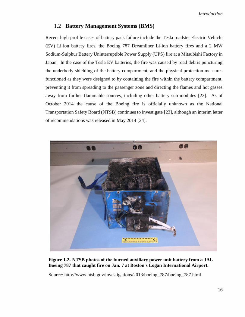
Recent high-profile cases of battery pack failure include the Tesla roadster Electric Vehicle
(EV) Li-ion battery fires, the Boeing 787 Dreamliner Li-ion battery fires and a 2 MW
Sodium-Sulphur Battery Uninterruptible Power Supply (UPS) fire at a Mitsubishi Factory in
Japan. In the case of the Tesla EV batteries, the fire was caused by road debris puncturing
the underbody shielding of the battery compartment, and the physical protection measures
functioned as they were designed to by containing the fire within the battery compartment,
preventing it from spreading to the passenger zone and directing the flames and hot gasses
away from further flammable sources, including other battery sub-modules [22]. As of
October 2014 the cause of the Boeing fire is officially unknown as the National
Transportation Safety Board (NTSB) continues to investigate [23], although an interim letter
of recommendations was released in May 2014 [24].
Figure 1.2- NTSB photos of the burned auxiliary power unit battery from a JAL
Boeing 787 that caught fire on Jan. 7 at Boston's Logan International Airport.
Source: http://www.ntsb.gov/investigations/2013/boeing_787/boeing_787.html

Introduction
17
The 2 MW Sodium Sulphur Battery UPS fire at Mitsubishi took eight and a half hours to
bring under control and a further two weeks to extinguish. The fire was caused by the failure
of a single cell module which itself was a part of a 384 cell battery pack. As the faulty cell
failed it leaked molten material, which caused a short between adjacent battery cells. The
resulting heat caused the whole battery to be compromised [25].
These cases highlight the importance and safety-critical function of the battery BMS and
physical protection measures. When a battery pack fails, even when it does so in a pre-
calculated and ‘safe’ manner such as in the case of the Tesla EV the result can be dangerous,
and highly damaging to the brand in terms of public perception. Thus we can observe three
distinct and significant damaging factors that may arise as a result of poor BMS and/or
physical protection measures:
Loss of/injury to life, and destruction of equipment
Underperformance of equipment and subsequent damage to public perception
Premature end of life (EOL) of battery
1.2.1 Function of the BMS
A BMS must perform three broad functions. These functions will be described in the context
of a large array of Li-ion cells assembled into a pack, such as is found in a typical Electric
Vehicle (EV) application.
Protect cells and battery packs from damage by keeping the battery within its Safe Operating
Area (SOA)
Arguably the most important task for the BMS is to maintain a battery pack in a safe state.
Battery packs consisting of parallel and series arrays of multiple cells can have very high
energy density and have the potential to deliver large fault currents, which could lead to
catastrophic temperature rises and cascading failure of the cells. Manufacturers minimise
this risk by creating sub-modules within larger battery packs, with features such as physical
firewalls and fuses between modules, vents to control the direction of hot gasses and flames
in the event of fire, and armour plating to protect against puncturing [22].
In tandem to these physical safety measures, the BMS monitors pack electrical and thermal
conditions to ensure that individual cells are kept within specification. Upper and lower
Introduction
18
voltage limits, maximum continuous charge/discharge currents and pulse currents are
chemistry-specific and given in cell manufacturers datasheets alongside operational
temperature ranges.
Maintain the battery to meet the requirements of its application
The operating conditions just described are those which must be adhered to in order to
maintain safe functioning of the battery pack. Ensuring that these limits are enforced is a
coarse function of the BMS, but its value extends beyond safety and the BMS may perform
secondary and tertiary functions depending on the application. For instance the BMS in a
laptop will alert the user when the State of Charge (SoC) reaches a critically low level. Once
the SoC drops to a predefined level then the BMS might switch to energy saving mode,
disabling inessential services before eventually taking control from the user and executing a
safe shutdown sequence in order that the system be put into a safe state while there is still
battery power to do so. Then the BMS isolates the battery from any new demands until it
has been recharged to a predefined minimum SoC.
Maintain the cells and battery packs to maximise the lifetime of the battery
A third function of the BMS is to prolong the useable life of the battery. Observing safety
limits and application-specific functional limits may be considered the primary and
secondary tasks for the BMS, while a useful tertiary task is to extend the life of the battery
pack. There may be some overlap between the secondary and tertiary function of the BMS,
and the mechanisms it uses to achieve these include battery equalisation, heating, cooling
and controlling the distribution of load demand amongst the cells.
1.2.2 Key Estimation Metrics
An important branch of battery research is that of estimating the state, or condition of the
battery at any given time. End users in many applications require accurate and reliable means
of assessing the State of Charge (SoC) of their battery; from mobile phone users and laptop
users through to Electric Vehicle (EV) drivers, Unmanned Aerial Vehicle (UAV) operators
and large plant (>1 MW Uninterruptible Power Supplies (UPS)).
Compare the task of estimating the remaining range of an Internal Combustion engine car,
based on the fuel available in the tank, with the same task of estimating the range of an
Introduction
19
Electric Vehicle based on the charge remaining in the battery. Clearly the biggest influence
on the range in each case will be the volume of fuel in the tank, and the amount of available
charge in the battery respectively. Measuring the quantity of fuel in a tank is a relatively
simple task and one that can be achieved with a high degree of accuracy. Furthermore, the
rate at which fuel is consumed has no effect on the remaining capacity. Measuring the charge
remaining in a battery is a more complex task; State of Charge of a battery is not a fixed
quantity but is dependent on variables such as temperature, rate of discharge/charge, cycle
history of the battery, and battery form factor among other things.
When measuring and/or estimating battery states, the measurable quantities are cell voltage,
current and temperature. These inputs are then often used to feed look-up-tables or estimator
algorithms, frequently based on knowledge of prior load-cycle history. Returning to the
examples given at the beginning of this section, mobile phone users will be aware of the
frustration arising from a bad estimator algorithm – when the phone charge indicator
suddenly jumps from 50 % to empty it does not necessarily follow that 50 % of the available
capacity has been used in a disproportionally short amount of time, but it may instead mean
that the estimation calculation is inadequate to cover all operating conditions. In the case of
an EV operator an insufficient SoC estimation algorithm may leave them stranded - a UAV
operator may lose their vehicle.

Introduction
20
1.2.2.1 Battery Metrics
Battery State-of-Charge, SoC is a measure of the remaining useful charge in a battery pack,
usually given as a percentage of maximum possible charge. The charge capacity of a battery
declines throughout its life-cycle therefore an accurate estimation of SoC requires that the
present maximum charge capacity of the battery be known, as well as the amount of useable
charge remaining. Therefore another metric is required to track these changes in charge
capacity – and feed the calculation of SoC estimates - as it decreases from the nominal
capacity of a new battery; Battery State-of-Health, SoH is a parameter that reflects the present
condition of an ageing battery in comparison with a new battery. As well as declining
capacity, other parameters change over the lifetime of a battery. Internal resistance increases,
maximum available power declines and the capability to support a given load is diminished.
A third useful metric is State-of-Function, SoF, which is a measure of the battery’s capability
to perform a specific duty in support of the functionality of a system which is powered by
the battery. SoF is a function of SoC, SoH and battery temperature.
Introduction
21
1.2.3 Battery State Estimation Tools
As battery technology develops and progresses, so too the techniques of estimating the
remaining charge have to be adapted. What works well when applied to one chemistry may
not be suitable for another, and for this reason there is a large amount of ongoing research
directed at estimation methods. Each time a new chemistry is developed - or even simply a
new form factor of the same cell chemistry – existing models and estimation techniques must
be updated.
The following is an overview of popular estimation tools which can be categorised into direct
methods, a book-keeping approach, and adaptive techniques which comprise several
estimation methods in combination.
1.2.3.1 Direct
Historically, battery state measurements began primitively with simple direct voltage
measurements.
The voltage drop across an external power resistor was measured and compared with the
unloaded terminal voltage. In a healthy battery the on-load voltage drop would be minimal,
while a large drop would indicate the need for the battery to be recharged or - in the case of
a primary battery - replaced. Over the years since these first techniques were developed in
1938 [26] a number of different methods of state estimation have been devised and often
used in combinations of two or more to improve the accuracy of the estimates. The most
widely employed direct measurement techniques are presented here.
1.2.3.1.1 Battery and Cell Voltage Measurements
As a battery becomes depleted the terminal voltage drops. It is reasonable to expect therefore
that terminal voltage might provide a good indicator of the SoC of a battery or cell, and
indeed it is possible to infer the SoC from this data, however the task is complicated by the
fact that the voltage is heavily dependent on cell temperature and rate of charge/discharge. If
the cell temperature and discharge rate are both known then the error can be corrected, albeit
at the expense of increased cost and processing complexity without any significant
advantages over other available approaches such as coulomb counting.
Introduction
22
1.2.3.1.2 Electromotive Force (EMF)
The EMF of a Li-ion battery (the open circuit voltage, OCV, under steady-state, no-load
conditions) can be used as a SoC metric, since the relationship between SoC and EMF is
nearly constant over the lifetime of a battery and there is only a small temperature dependence
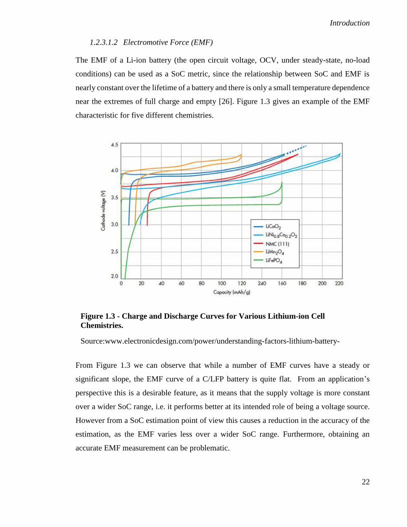
near the extremes of full charge and empty [26]. Figure 1.3 gives an example of the EMF
characteristic for five different chemistries.
From Figure 1.3 we can observe that while a number of EMF curves have a steady or
significant slope, the EMF curve of a C/LFP battery is quite flat. From an application’s
perspective this is a desirable feature, as it means that the supply voltage is more constant
over a wider SoC range, i.e. it performs better at its intended role of being a voltage source.
However from a SoC estimation point of view this causes a reduction in the accuracy of the
estimation, as the EMF varies less over a wider SoC range. Furthermore, obtaining an
accurate EMF measurement can be problematic.
Figure 1.3 - Charge and Discharge Curves for Various Lithium-ion Cell
Chemistries.
Source:www.electronicdesign.com/power/understanding-factors-lithium-battery-
equation
Introduction
23
The current demand on the battery must be reduced to zero in order to make an accurate, off-
line EMF measurement. This voltage relaxation method of obtaining the internal driving
force of the battery requires a time period of off-line battery relaxation – typically 3 hours
for C/LFP - to allow the battery voltage to reach steady-state; the required relaxation time is
extended significantly if the battery has been subjected to a high load current, low
temperature, or if it is near fully discharged. For many applications this rules out the use of
voltage relaxation as a method of obtaining the EMF.
An EMF approximation may also be obtained by linear extrapolation of terminal voltages
measured under different load current rates, thereby approximating the terminal voltage at
zero current, but a further complication in the case of some batteries - such as C/LFP and Ni-
MH - is that the measured OCV exhibits a hysteresis effect which is dependent on whether
the battery is being charged or discharged [27] (see Figure 1.3 for an example of cell voltage
hysteresis). Knowledge of cycle history may also be required in these cases unless an
adaptive method is also implemented [28] (see section 2.3.3).
Linear interpolation may be used to determine the mean battery voltage over two consecutive
charge/discharge cycles, thereby nulling the effects of hysteresis.
Two practical SoC estimation techniques involving the use of EMF data are the look-up table
and the piecewise linear function. The look-up table is based on laboratory measurements of
SoC values stored alongside corresponding EMF data. In the laboratory accurate SoC can
easily be determined by running a full discharge or charge test on a battery, but this is of no
practical use in an online situation when the battery is in use. Instead, the results of prior full
charge/discharge cycles done in the laboratory are used to populate look-up tables. Clearly
the look-up table approach will yield the best results when it includes more data points, but
again this increases the complexity and expense of the process involved.
The piecewise linear function is a compromise between the accuracy of the look-up table and
the expense of including an exhaustive data-set. The EMF curve here is approximated with
piecewise linear functions, and the accuracy of the SoC measurements obtained is dependent
on the number of intervals chosen.
Introduction
24
1.2.3.1.3 Model-based SoC Estimation
The model-based approach to estimation removes the requirement for direct offline EMF
measurement by taking into account the internal resistance of the cell or battery pack. Models
can be broadly classified into three types: First principle models, Equivalent circuit models,
and Black-box models [29].
Equivalent circuit models are often used [30–47] which express the relationship between
EMF and dynamic data in terms of the linear differential equations of RC circuits and
discrete-time dynamic equations of the cell model [44].
1.2.3.1.4 Impedance Measurements
Impedance measurements over a wide range of frequencies can provide a means of
identifying the physiochemical processes in an electrochemical system. Electrochemical
Impedance Spectroscopy (EIS) allows equivalent circuit parameters to be extracted which in
turn may be correlated with physiochemical processes within cells.
As a battery is discharged, observed changes in the impedance spectrum can be used to
identify SoC. Also, changes in impedance can be correlated to ageing effects within the
battery and therefore feed SoH and SoF estimations.
Impedance measurements and analysis form the main body of the author’s work, and will be
discussed in more detail in section 3.
1.2.3.2 Book-keeping (Coulomb Counting)
This approach to indicating battery SoC relies on monitoring the charge flowing in or out of
the battery. Battery current is continuously measured and integrated, while other battery data
may also be used to feed the book-keeping system and compensate for temperature effects,
cycle life and self-discharge rate. Equation 1 is an example of a SoC calculation that is based
on knowledge of prior SoC at time t0, SoC0, the nominal capacity of the battery, Cn, and the
battery current I. The coulombic efficiency η varies with temperature, battery current, SoC,
and SoH.
Introduction
25
0
0
1t
n t
I dC
SoC SoC
Equation 1
Inspection of Equation 1 reveals some weaknesses in this method. Any errors in measuring
either coulombic efficiency (η) or battery current (I) will produce a cumulative error in the
SoC result, while an error in the initial SoC0 carries through and affects the precision of the
final SoC estimation. The precision of this method is reliant on the precision of the current
sensor, the acquisition frequency, and frequent calibration checks to ensure that SoCo is
accurate and to compensate for any errors in the estimation of η. Nevertheless the book-
keeping approach is widely used, with the shortcomings described here compensated for by
use of other techniques, such as using an adaptive algorithm to prevent errors becoming
cumulative.
1.2.3.3 Adaptive
As has been described here, the remaining useful charge in a battery is highly dependent on
future demand and operating conditions, which in some cases such as a portable music player
may be easy to predict while in others, such as EVs, can be highly unpredictable. For this
reason, if the implementation cost (processing and monetary costs) can be justified then an
adaptive approach may be taken, often comprising more than one measurement type – for
example an OCV approximation method may be combined with coulomb counting, and an
adaptive approach would compare the resulting estimated values with observed response and
inform the new estimates accordingly.
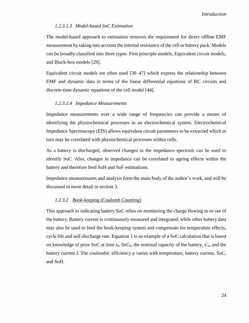
1.2.3.3.1 Fuzzy Logic
The Fuzzy Logic (FL) system uses subjective rules to produce ‘crisp’ outputs from data sets
having uncertain values (‘fuzzy’ sets). A cell voltage, absolute temperature, or load current
would all be considered ‘crisp’ data, whereas fuzzy sets have less certain categories of data.
A fuzzy set might include the subsets ‘Poor’ or ‘Very Poor’ to describe SoH (see Figure 1.4),
and an element of the set ‘SoH’ might belong to different subsets by various degrees of
‘membership’. Identifying the fit of real-valued data into this fuzzy set is called the
‘fuzzification’ of the data.
Introduction
26
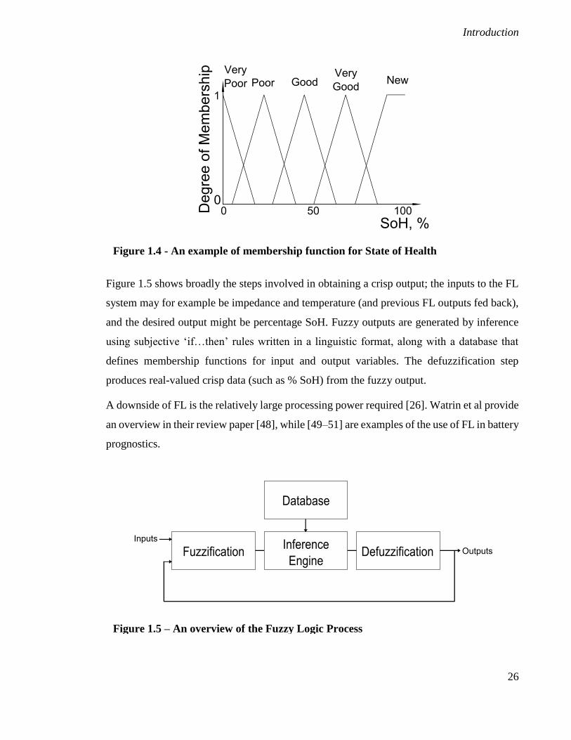
Figure 1.5 shows broadly the steps involved in obtaining a crisp output; the inputs to the FL
system may for example be impedance and temperature (and previous FL outputs fed back),
and the desired output might be percentage SoH. Fuzzy outputs are generated by inference
using subjective ‘if…then’ rules written in a linguistic format, along with a database that
defines membership functions for input and output variables. The defuzzification step
produces real-valued crisp data (such as % SoH) from the fuzzy output.
A downside of FL is the relatively large processing power required [26]. Watrin et al provide
an overview in their review paper [48], while [49–51] are examples of the use of FL in battery
prognostics.
Figure 1.4 - An example of membership function for State of Health
Figure 1.5 – An overview of the Fuzzy Logic Process
Introduction
27
1.2.3.3.2 Artificial Neural Network (ANN)
A key advantage of the neural network model is that it can be universally applied, irrespective
of the battery chemistry. SoC is estimated using the non-linear mapping characteristics of the
neural network [52], and the construction of the model does not need to include the prior
input of battery-specific information; indeed, because of the large amount of training data
that is required the ANN model can also reveal SoH information, but it is the large amount
of training information (typically upwards of 1000 cycles [53]) that is a key disadvantage of
this method. Processing power may also be a limiting factor to implementation, however
some of the advantages of the ANN approach are obtainable without the need for complex
processing if the adaptive aspect is not required [53] to estimate individual behaviour.
1.2.3.3.3 Kalman Filter (KF) and Extended Kalman Filter (EKF)
This method uses an algorithm which can estimate system states that are not directly
measurable, such as SoC or SoH, and can also be useful in minimising measurement noise
effects [48]. Kalman Filters are used in the analysis of stochastic and linear signals, but
adaptations can be made to allow their use in solving non-linear problems such as those
presented by battery SoC estimation, one of which is the Extended Kalman Filter (EKF).
Examples of successful application of these filters in the online estimation of SoC and SoH
of lead-acid batteries can be found in [54–58].
The algorithm comprises several equations that estimate a measurable value which is then
compared to a real measurement of the value and the estimated value is subsequently
corrected. Accurate cell models must be developed, and these are often simplified equivalent
circuit models with minimal parameters to ensure a fast computing process.
Introduction
28
1.3 Electrochemical Impedance Spectroscopy (EIS)
As mentioned previously, EIS allows equivalent circuit parameters to be extracted which in
turn may be correlated with physiochemical processes within cells. Detailed electrochemical
models are often not required, and are themselves problematic in embedded applications due
to their complexity – see [59].
Observed changes in the impedance spectrum of a cell can be used to identify SoC and can
also be correlated to ageing effects within the battery, thus feeding SoH and SoF estimations.
Here we look at this relationship.
1.3.1 The Relationship between Battery Impedance and Battery Dynamics
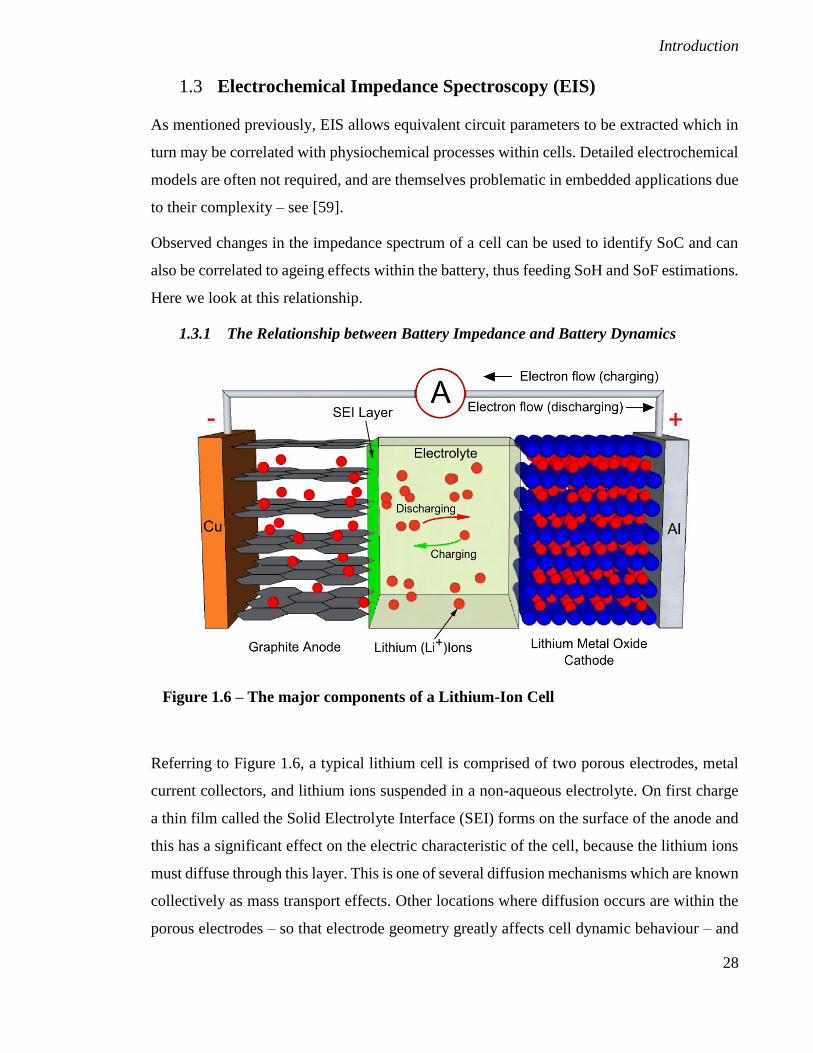
Referring to Figure 1.6, a typical lithium cell is comprised of two porous electrodes, metal
current collectors, and lithium ions suspended in a non-aqueous electrolyte. On first charge
a thin film called the Solid Electrolyte Interface (SEI) forms on the surface of the anode and
this has a significant effect on the electric characteristic of the cell, because the lithium ions
must diffuse through this layer. This is one of several diffusion mechanisms which are known
collectively as mass transport effects. Other locations where diffusion occurs are within the
porous electrodes – so that electrode geometry greatly affects cell dynamic behaviour – and
Figure 1.6 – The major components of a Lithium-Ion Cell
Introduction
29
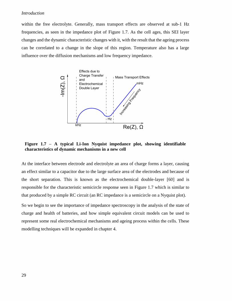
within the free electrolyte. Generally, mass transport effects are observed at sub-1 Hz
frequencies, as seen in the impedance plot of Figure 1.7. As the cell ages, this SEI layer
changes and the dynamic characteristic changes with it, with the result that the ageing process
can be correlated to a change in the slope of this region. Temperature also has a large
influence over the diffusion mechanisms and low frequency impedance.
At the interface between electrode and electrolyte an area of charge forms a layer, causing
an effect similar to a capacitor due to the large surface area of the electrodes and because of
the short separation. This is known as the electrochemical double-layer [60] and is
responsible for the characteristic semicircle response seen in Figure 1.7 which is similar to
that produced by a simple RC circuit (an RC impedance is a semicircle on a Nyquist plot).
So we begin to see the importance of impedance spectroscopy in the analysis of the state of
charge and health of batteries, and how simple equivalent circuit models can be used to
represent some real electrochemical mechanisms and ageing process within the cells. These
modelling techniques will be expanded in chapter 4.
Figure 1.7 – A typical Li-Ion Nyquist impedance plot, showing identifiable
characteristics of dynamic mechanisms in a new cell
Introduction
30
1.3.2 Standard Laboratory EIS Techniques
1.3.2.1 Swept Frequency Sine
The most common, standard approach to measuring impedance is to measure the system
response to a small voltage or current stimulus of fixed frequency. The phase and amplitude
of the response can easily be manipulated using fast Fourier transform (FFT) techniques to
give the impedance as a function of frequency. An impedance spectrum of the system can be
constructed by repeating the test over a range of frequencies; commercial instruments are
available that sweep the frequency in the range of typically 1 mHz to 1 MHz, and directly
produce an impedance spectrum in the form of a bode diagram or a Nyquist plot. The signal
to noise ratio of this method is excellent - since frequencies of interest can be directly
specified – however the measurement time required can be prohibitively long when low
frequency data is needed [61]; low frequency response is an important aspect of the frequency
response function (FRF) of an electrochemical cell [60].Ω
1.3.2.2 Transient Measurements
Another method involves applying a voltage step-function (this is potentiostatic mode; in
galvanostatic mode a current step-function is used instead) V (t<0, V=0; t>0, V=V0) to the
battery and measuring the resultant time-varying current i(t). The quantity V0/i(t) is often
called the indicial impedance, or time-varying resistance [62], and usually transformed into
the frequency domain to show the frequency dependent impedance. The excitation in this
case is non-periodical and therefore a suitable windowing function must be used to correct
distortion in the impedance spectra. Another requirement is that V0 is kept sufficiently small
that a linear system response is ensured.
1.3.2.3 White Noise Stimulation and Broadband Excitation
A signal composed of true white (random) noise will stimulate a system equally at all
frequencies. Furthermore, this description can be relaxed to say that the requirement for a
stimulus to be considered a white noise input to a system is that it has a flat power density
spectrum over a frequency range much greater than the system bandwidth [63]. A stimulus
of this type (i.e. one possessing a uniform power spectrum) will produce a system response
Introduction
31
that can readily be manipulated into providing the system frequency response using Fourier
analysis.
There are three important advantages to this method of system identification over the two
conventional methods described above [63]:
1. The system (battery) may be allowed to remain in its normal functioning mode, since
the noise excitation is spread over a wide bandwidth and is necessarily of a low
intensity so that the system is maintained operating within its linear region.
2. Measurements are not affected by other sources of noise, provided they are
stochastically independent of the input noise source.
3. Stored energy in the system has no effect on the measurement of the impulse
response.
However, there are two important disadvantages to this method. Accurate estimates of the
cross-correlation function still require that the stimulus and response are measured for a long
(ideally infinite) amount of time. Second, the stimulus energy must be kept small to ensure
an approximately linear response is measured from a non-linear system. This increases the
accuracy required in the measurement of the stimulus and response signals.
The measurement of the frequency response function (FRF) via broadband excitations has
been demonstrated to take significantly less time than when using stepped sinusoidal
excitation [64], given good signal-to-noise ratio (SNR) (this time advantage is reduced when
the SNR is poor).
1.3.3 Pseudo-Random Binary Sequences (PRBS) as Pseudo-White Noise Input
A pseudo-random noise source produces a frequency response that is similar to white noise
except that it is produced deterministically and is therefore periodic, and the power spectral
response is therefore only flat across a specific bandwidth; it is considered to be a source of
band-limited white noise.
A key reason for the early adoption and continued success of PRBS is that the signal can be
generated easily with a minimum of digital hardware using simple shift register circuitry and
appropriate feedback (see Figure 1.8). While several classes of pseudo-random binary
Introduction
32
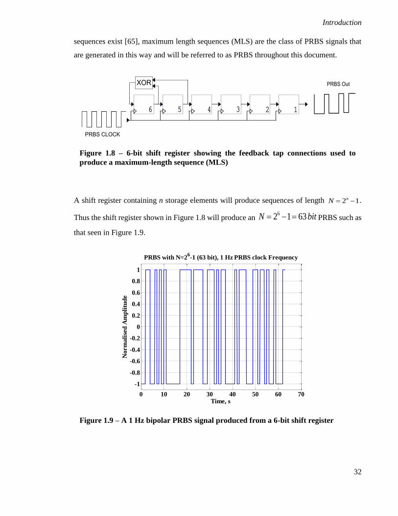
sequences exist [65], maximum length sequences (MLS) are the class of PRBS signals that
are generated in this way and will be referred to as PRBS throughout this document.
A shift register containing n storage elements will produce sequences of length 2 1nN .
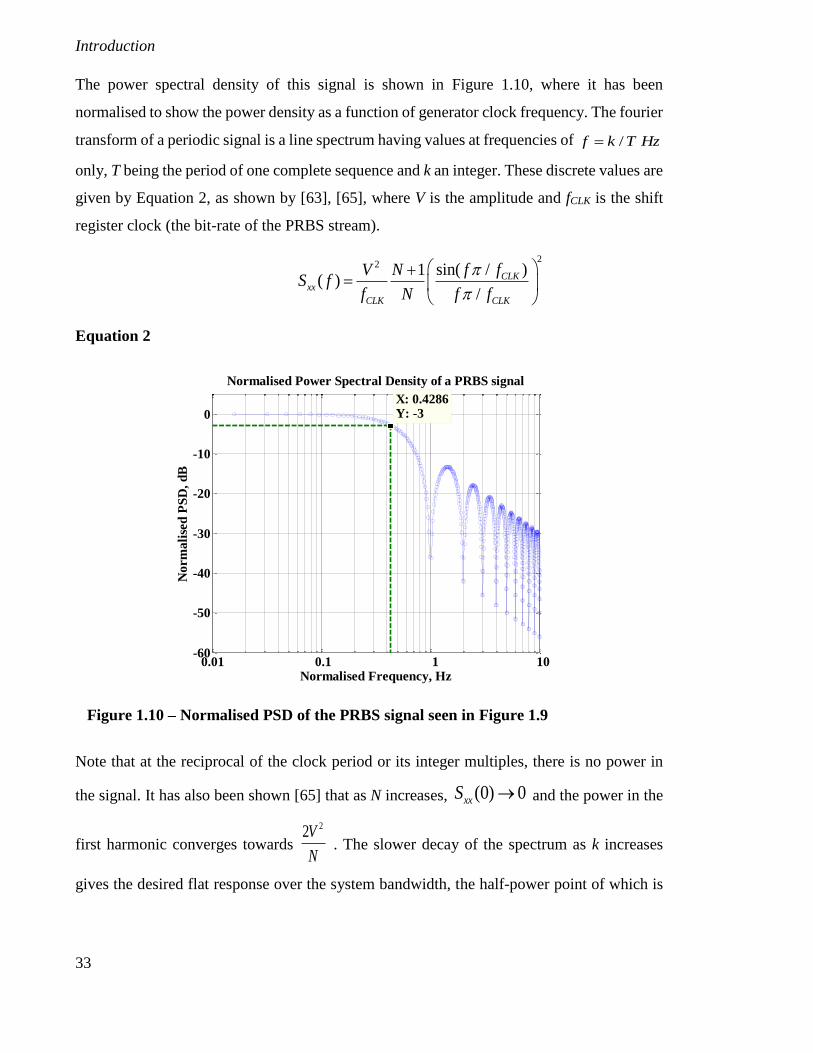
Thus the shift register shown in Figure 1.8 will produce an 62 1 63N bit PRBS such as
that seen in Figure 1.9.
Figure 1.8 – 6-bit shift register showing the feedback tap connections used to
produce a maximum-length sequence (MLS)
Figure 1.9 – A 1 Hz bipolar PRBS signal produced from a 6-bit shift register
0 10 20 30 40 50 60 70
-1
-0.8
-0.6
-0.4
-0.2
0
0.2
0.4
0.6
0.8
1
Time, s
No
rm
ali
sed
Am
pli
tud
e
PRBS with N=26-1 (63 bit), 1 Hz PRBS clock Frequency
Introduction
33
The power spectral density of this signal is shown in Figure 1.10, where it has been
normalised to show the power density as a function of generator clock frequency. The fourier
transform of a periodic signal is a line spectrum having values at frequencies of /f k T Hz
only, T being the period of one complete sequence and k an integer. These discrete values are
given by Equation 2, as shown by [63], [65], where V is the amplitude and fCLK is the shift
register clock (the bit-rate of the PRBS stream).
22 sin( / )1
( )/
CLKxx
CLK CLK
f fV NS f
f N f f
Equation 2
Note that at the reciprocal of the clock period or its integer multiples, there is no power in
the signal. It has also been shown [65] that as N increases, (0) 0xxS and the power in the
first harmonic converges towards
22V
N . The slower decay of the spectrum as k increases
gives the desired flat response over the system bandwidth, the half-power point of which is
Figure 1.10 – Normalised PSD of the PRBS signal seen in Figure 1.9
0.01 0.1 1 10-60
-50
-40
-30
-20
-10
0
X: 0.4286Y: -3
Normalised Frequency, Hz
No
rm
ali
sed
PS
D,
dB
Normalised Power Spectral Density of a PRBS signal
Introduction
34
approximately 0.443 CLKf . In Figure 1.10 above this value is 0.429, as the PSD was
produced by an N=63 (6-bit) PRBS shift register.
As stated previously, this method of system identification offers an advantage in the ability
to stimulate many frequencies simultaneously with even power, reducing measurement time.
A battery or cell can more easily be kept within a linear region of operation throughout the
identification process, and the impedance spectrum is easily obtained by dividing the power
spectrum of the voltage response with that of the current stimulus (assuming a current
controlled excitation). Examples of the technique can be found in [66], [67].
1.4 Conclusions
A brief history of popular EV battery chemistries has been presented, along with a description
of Battery Management Systems and state estimation techniques. PRBS methods of EI
Spectroscopy have been introduced, forming a motive for the work presented in the next
chapters. In Chapter 2 there is a description of the equipment that was developed for purposes
of charge cycling and impedance measurement of a range of Li-ion cells. The results of tests
on two types of cell, LFP 26650E 3 Ah cells and LTO polymer 100 Ah pouch cells, are
presented. The author’s main findings from the early work precede Chapter 3, which gives
details of the new hardware – and corresponding control software - that was developed to
address the weaknesses of the first designs. Concluding remarks and suggestions for further
work are given in Chapter 4.
.
35
Chapter 2: Battery Charge Cycler and PRBS Impedance
Measurement System
2.1 Objectives
As part of a TSB funded battery project, a test rig capable of cycling Li-ion cells, and
measuring their impedance using PRBS as an EIS stimulus was to be built. As there was
some pre-existing hardware that could be modified and re-purposed, the task was split into
two parts – high current charge cycling, and low current PRBS measurements.
The high current cycling rig was intended to be capable of testing a single Li-ion cell
(nominal voltage < 10 V) at pulse currents up to 150 A, and charge cycling the cells at a
lower rate of up to 50 A continuously. A PID controlled temperature environment was
supplied so that tests could be conducted at temperatures in the range -10ᵒ C to 50ᵒ C. The
intention was to test actual cell capacities when cycled at a rate of C/2 (C being nominal cell
capacity - e.g. 3 Ah - and the ‘C rate’ being C/1 hour - e.g. 3 A), and identify the maximum
current a cell could accept before reaching maximum/minimum permitted voltages at various
SoC (10 % increments). PRBS impedance tests would also be done at each SoC and
temperature. Later uses included testing battery packs up to 28.8 V (24 V nominal LFP
packs).
The high current rig was used to cycle the cells and bring them to a known SoC. With a cell
discharged to a known SoC, the cell could then be taken offline from the high current rig and
a PRBS impedance test performed using the smaller rig; the SoC of the cell must not be
changed significantly as a result of the impedance test, therefore only low currents could be
used to measure the impedance. The system identification aspect of the test relies on being
able to make a linear approximation of the non-linear cell.
Therefore, the focus here will be on the procedures that were followed during this phase of
the work; there is a critique at the end of the chapter that will hopefully illuminate some of
the decisions and changes that were made, prior to later work.
Battery Charge Cycler and PRBS Impedance Measurement System
36
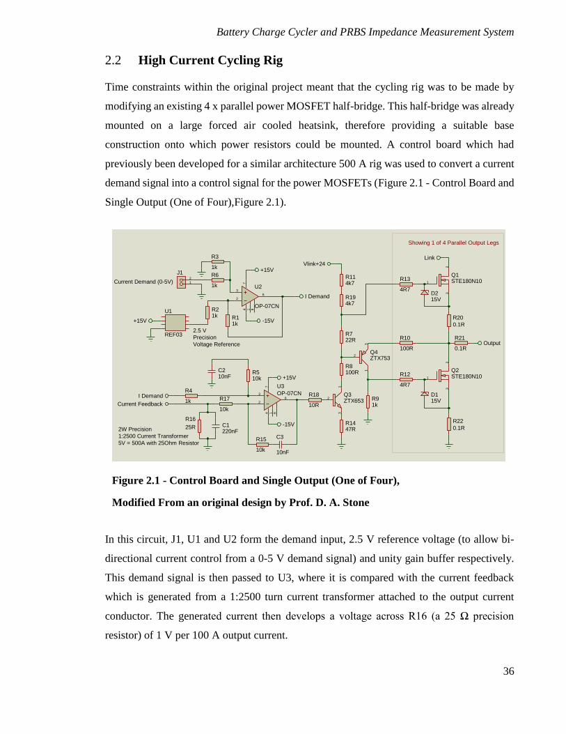
2.2 High Current Cycling Rig
Time constraints within the original project meant that the cycling rig was to be made by
modifying an existing 4 x parallel power MOSFET half-bridge. This half-bridge was already
mounted on a large forced air cooled heatsink, therefore providing a suitable base
construction onto which power resistors could be mounted. A control board which had
previously been developed for a similar architecture 500 A rig was used to convert a current
demand signal into a control signal for the power MOSFETs (Figure 2.1 - Control Board and
Single Output (One of Four),Figure 2.1).
In this circuit, J1, U1 and U2 form the demand input, 2.5 V reference voltage (to allow bi-
directional current control from a 0-5 V demand signal) and unity gain buffer respectively.
This demand signal is then passed to U3, where it is compared with the current feedback
which is generated from a 1:2500 turn current transformer attached to the output current
conductor. The generated current then develops a voltage across R16 (a 25 Ω precision
resistor) of 1 V per 100 A output current.
Figure 2.1 - Control Board and Single Output (One of Four),
Modified From an original design by Prof. D. A. Stone
3
2
74
6
1 8
U3
OP-07CN
R16
25R2W Precision
1:2500 Current Transformer
5V = 500A with 25Ohm Resistor
R17
10k
R510k
R15
10k
C3
10nF
C210nF
R4
1kCurrent Feedback
I Demand R18
10R
R1447R
R8100R
R722R
R194k7
R114k7
Vlink+24
R91k
R10
100R
R12
4R7
D115V
Output
R13
4R7D215V
+15V
-15V
3
2
74
6
1 8
U2
OP-07CNU1
REF032.5 V
Precision
Voltage Reference
+15V
R21k
+15V
-15V
1
2
J1
Current Demand (0-5V)
R6
1k
R11k
R3
1k
I Demand
2
13
Q4ZTX753
2
13
Q3ZTX653
C1220nF
2
1
3
Q2STE180N10
2
1
3
Q1STE180N10
Link
Showing 1 of 4 Parallel Output Legs
R20
0.1R
R21
0.1R
R22
0.1R
Battery Charge Cycler and PRBS Impedance Measurement System
37
The output of U3 feeds the gate drive circuit formed by Q3, Q4, and their associated resistor
network. This circuit ensures that both high and low side MOSFETs can turn fully off (the
network is fed by a voltage 24 V above the DC link voltage), and eliminates the possibility
of shoot-through occurring since only one set of output devices (high or low) may be
conducting at any time.
The output MOSFETs are each rated for 120 A continuous drain current at 100ᵒ C (540 A
pulsed), and 450 W total dissipation at 25ᵒ C. As there were four parallel channels mounted
on a large forced-air heatsink, this was deemed sufficient for our purposes (150 A pulses)
with no further calculations. The system was tested up to a link voltage of 35 V, to allow
testing of 24 V nominal LFP batteries (28.8 V max battery under test voltage).
Acquisition of charge cycling signals (cell current and terminal voltage) is done using a NI
USB 6009 14-bit DAQ, at a sample rate of 100 Hz.
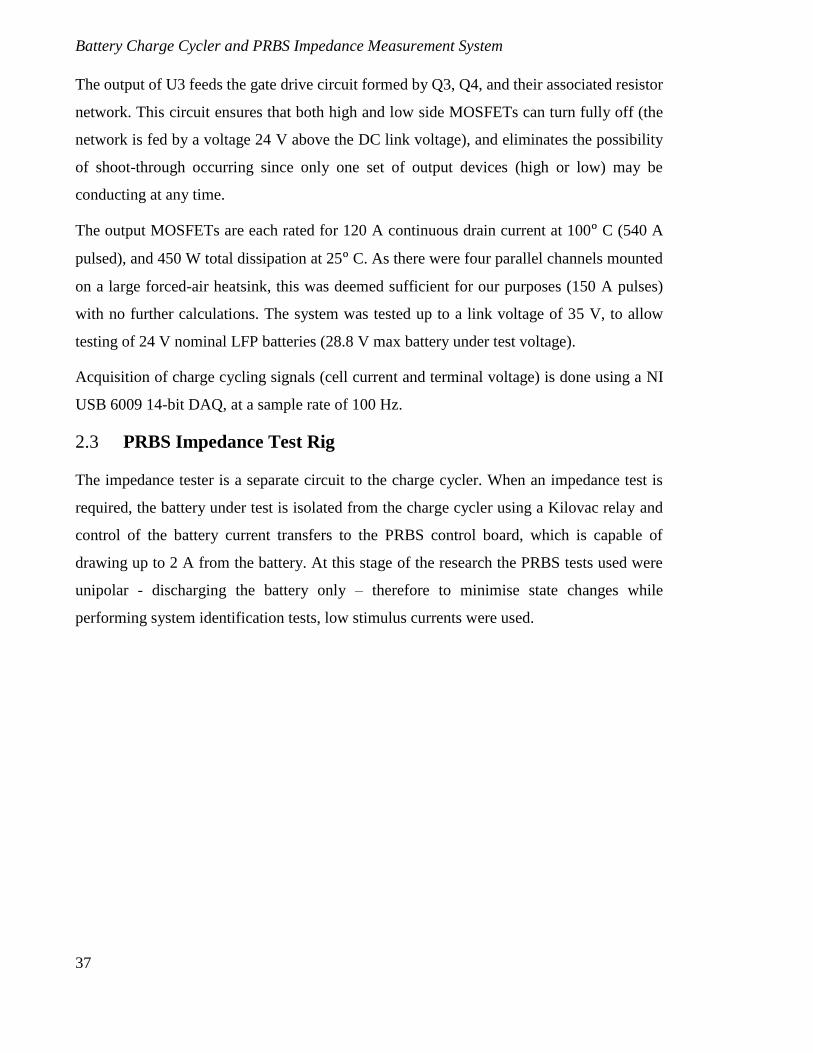
2.3 PRBS Impedance Test Rig
The impedance tester is a separate circuit to the charge cycler. When an impedance test is
required, the battery under test is isolated from the charge cycler using a Kilovac relay and
control of the battery current transfers to the PRBS control board, which is capable of
drawing up to 2 A from the battery. At this stage of the research the PRBS tests used were
unipolar - discharging the battery only – therefore to minimise state changes while
performing system identification tests, low stimulus currents were used.
Battery Charge Cycler and PRBS Impedance Measurement System
38
The circuit in Figure 2.2 shows the initial design of the PRBS test circuit. The digital PRBS
stream is generated using an Arduino ATmega 2560 based microcontroller producing 0 V
(low) and 5 V (high) on a digital pin as it sequentially reads each bit from a 63-bit PRBS
sequence stored in memory. Different PRBS clock frequencies are generated by specifying
the delay time of a loop which steps through the sequence in memory.
Stability problems in early testing meant that the current feedback arrangement shown was
changed; R8 was used to provide 1 V/A feedback for the control loop, while the output of
U1 was reserved purely for current measurement purposes. RV1 is used to scale the input
demand signal so that a 5 V (high) input produces 1 A discharge current in the battery.
During impedance testing, control of the current demand and data acquisition is transferred
to a MATLAB script which sends a start trigger to the Arduino, and begins streaming
acquisition on a LabJack U6. The U6 was configured to acquire differential current and
voltage readings (total of four channels) at 5 kS/s, at which rate it is capable of 14-bit
resolution.
Figure 2.2 – PRBS load control
R5
100R
C210n
C310n
+15
-15
IN
OUT
1
60V
8
V+9
Out7
2
3
5
4
U3
LTS-15-NPCurrent Sensor
125 mV/A
2.5 V = 0 A
Q1IRF510
3
2
6
74 1 5
U2
TL081
1
2
J1
Test Battery
FU1
1AR316k
R410k
SCALED TERMINAL VOLTAGE
CURRENT FEEDBACK
+5
R1
10k
R6
10k
1
2
J2
Digital PRBS stream1
2
3
RV1
T63 MULTI TURN POT
C110n
C410n
+15
-15
3
2
6
74 1 5
U1
TL081
CURRENT FEEDBACK
R210k
R7
10k
PRBS Battery Interface
HRPrice 6-2-2012. Ver 2.
R81R7W Power Resistor
Battery Charge Cycler and PRBS Impedance Measurement System
39
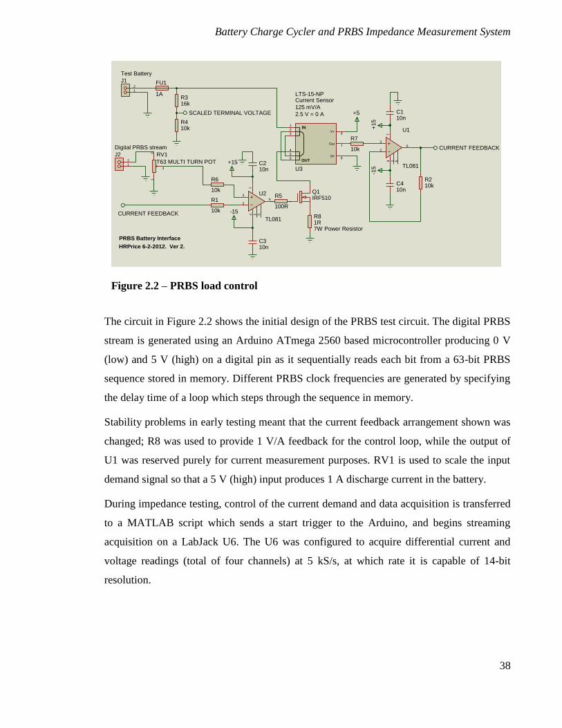
Figure 2.3 – Cycling Rig and PRBS Impedance Tester
Battery Charge Cycler and PRBS Impedance Measurement System
40
2.4 Test Procedure
The test method for measuring impedance at different SoC follows the following format.
Note that ‘C’ refers to the amp-hour capacity of the cell, thus a rate of 1C is equivalent to a
full charge or discharge in one hour (example values for 3 Ah LFP cells are used in
parentheses):
1. The cells are discharged at a C/2 rate until the low voltage cut-off (2.6 V) is reached.
2. Cells are charged at a C/2 rate up to their maximum voltage cut off, and held there
until the current reduces to a value of 3 % of C (90 mA for a 3Ah cell).
3. The cells are again discharged at C/2 rate until they reach the low voltage cut-off
(2.6 V for LFP cells).
4. Step 2 is repeated, and the cell is now considered to be at 100 % SoC.
5. The cell is taken offline for a set amount of time (at least 30 minutes, preferably of
the order of hours). This is the relaxation (rest) time, which allows the terminal
voltage to settle to a steady state.
6. An OCV reading is taken, then the cell is brought back online.
7. A PRBS impedance test is begun. This is broken into eight separate sequences of the
same 63-bit MLS, at bit rates from 1 kHz to 1 Hz (see full description in section
2.5.1), which lasts 96 seconds. These are then repeated and it is the data from the
second set which is then used (as the cell terminal voltage has then settled from its
initial ‘on load’ voltage drop into a steady load state) making the total impedance test
time around 200 seconds.
8. The test then enters a repetitive cycle until the low voltage cut-off is reached:
a. The cell is discharged by 10 % of its nominal capacity (300 mAh for a 3 Ah
cell).
b. Taken offline for a preset rest period (e.g. 30 minutes – same as step 5).
c. PRBS impedance test.
9. Once the cell has reached 0 % SoC (e.g. LFP cell terminal voltage reaches 2.6 V) step
8a is terminated and steps 8b and 8c are allowed to execute a final time.
10. The cell is re-charged to 30% SoC (ideal storage state for Li-ion cells).
Battery Charge Cycler and PRBS Impedance Measurement System
41
2.5 Impedance Tests
2.5.1 Stimulus Signals
The use of PRBS as a stimulus for EIS impedance measurement has been discussed in section
1.3. Table 2.1 shows the frequencies used and the resulting bandwidth of impedance
measurable from each sequence.
The test consists of two cycles of eight PRBS stimulus streams (16 total), and the post-
processing is done on the final eight sequences – this allows the cell to recover from the
initially severe voltage drop which results from being subjected to a load after being at rest.
Differential measurement of terminal response voltage and stimulus current is done at 5 kS/s.
2.5.2 Post-Processing
Following a typical test such as that outlined in Section 2.4, one data file for each impedance
test is generated. These contain the terminal voltage measured prior to the test, the SoC and
temperature of the cell, and a data array consisting of [time, stimulus current, and response
voltage]. The data array contains a continuous stream of all 16 sequences.
Sequence # PRBS Clock Frequency Useful Frequency
Range After
Processing
Test Duration for
63 bit PRBS
(single stream)
1 (9) 1 kHz 16 Hz – 330 Hz 63 ms
2 (10) 143 Hz 2.3 Hz – 47 Hz 440 ms
3 (11) 111 Hz 1.8 Hz – 37 Hz 570 ms
4 (12) 55.6 Hz 0.9 Hz – 18 Hz 1.13 s
5 (13) 25 Hz 0.4 Hz – 8.3 Hz 2.52 s
6 (14) 12.8 Hz 0.25 Hz – 4.2 Hz 4.91 s
7 (15) 4 Hz 65 mHz – 1.3 Hz 15.8 s
8 (16) 1 Hz 16 mHz – 330 mHz 63 s
Table 2.1 – Chosen PRBS Clock Frequencies and Resultant Bandwidth of
Spectrum
Battery Charge Cycler and PRBS Impedance Measurement System
42
The following is an outline of the process involved in generating an impedance spectrum
from a single set of 8 PRBS stimulus and response signals, the results of which follow in the
next chapter.
1. In order to identify the complete data sequences exactly, the 16 individual stimulus
and response signals are extracted from the data array by cross-correlating the array
with a clean reference signal for each PRBS clock frequency. The final set of eight
sequences are used.
2. A DFT of the current and voltage, yields a signal power spectrum for each sequence.
3. The impedance spectrum (now in the frequency domain) is obtained by V/I.
4. The obtained spectrum is band limited to the useful frequency ranges listed in Table
2.1.
5. The eight spectrums are combined and averaged to yield the impedance spectrum for
the cell.
2.6 Results
The primary purpose of the work was to characterise various 3.2 V - 3 Ah 26650E LiFePO4
cells, although the intention was that the equipment be versatile enough to test other cells,
such as 24 V - 20 Ah LFP battery packs, 100 Ah – 3.7 V LTO polymer (pouch) SLPB cells,
and 6 V – 24 Ah lead-acid batteries.
Presented here is a summary of the early tests done on the 26650E LFP cells, and the high
capacity SLPB LTO cells. In both cases impedance vs. SoC tests were run, along with basic
SoH tests done by comparing the impedance spectrums of a new cell and an aged cell.
Following the presentation of the results of this early work is a discussion of the problems
encountered and the weaknesses found in the test methods and resulting data.
Battery Charge Cycler and PRBS Impedance Measurement System
43
2.6.1 26650E LiFePO4 (LFP) Cells
These 3 Ah cells have a nominal voltage of 3.2 V. Table 2.2 lists the condition of the cells
and the test configuration used (single or parallel), along with the reference numbers used in
this section. Note that cell 1 was damaged during testing and was therefore only tested at
10°C, 20°C and 30°C. All other cells and configurations were tested to 50°C.
2.6.1.1 Discharge data
A typical pulsed current discharge (PDC) curve is shown in Figure 2.4. Offline time between
pulses was not recorded, which is why the current appears to be continuous and there are
visible peaks in the voltage curve, when in reality there is a 30 minute (1800 seconds) offline
period prior to each voltage peak. The test procedure was changed to log data continuously
in later work; this and other changes are discussed in more detail in section 2.7 - clearly it is
valuable to be able to analyse the recovery of the terminal voltage after a discharge pulse.
Figure 2.5 shows typical recharge curves for the LFP cells. Note that the scales are different
to the previous figure.
Cell Reference # Description
1 New cell, damaged during testing – incomplete dataset (< 30 cycles)
2 New cell – lightly cycled (< 30 cycles)
3 New cell – lightly cycled (< 30 cycles)
4 New cell (0 cycles)
5 End of Life (EOL) cell (2300 cycles)
23 Cells 2 and 3 in Parallel
234 Cells 2,3 and 4 in Parallel
Table 2.2 - Cell Reference Table
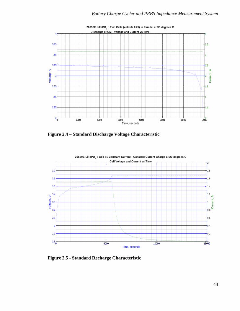
Battery Charge Cycler and PRBS Impedance Measurement System
44
Figure 2.4 – Standard Discharge Voltage Characteristic
0 1000 2000 3000 4000 5000 6000 70002
2.25
2.5
2.75
3
3.25
3.5
3.75
4
26650E LiFePO4 : Two Cells (cellrefs 2&3) in Parallel at 30 degrees C
Discharge at C/2. Voltage and Current vs Time
Vo
lta
ge
, V
Time, seconds0 1000 2000 3000 4000 5000 6000 7000
0
0.5
1
1.5
2
2.5
3
3.5
4
Cu
rre
nt, A
Figure 2.5 - Standard Recharge Characteristic
0 5000 10000 150002.8
2.9
3
3.1
3.2
3.3
3.4
3.5
3.6
3.7
Vo
lta
ge
, V
Time, seconds
26650E LiFePO4 : Cell #1 Constant Current - Constant Current Charge at 20 degrees C
Cell Voltage and Current vs Time
0 5000 10000 150000
0.2
0.4
0.6
0.8
1
1.2
1.4
1.6
1.8
2
Cu
rre
nt, A
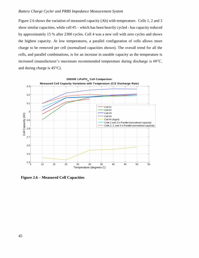
Battery Charge Cycler and PRBS Impedance Measurement System
45
Figure 2.6 shows the variation of measured capacity (Ah) with temperature. Cells 1, 2 and 3
show similar capacities, while cell #5 – which has been heavily cycled - has capacity reduced
by approximately 15 % after 2300 cycles. Cell 4 was a new cell with zero cycles and shows
the highest capacity. At low temperatures, a parallel configuration of cells allows more
charge to be removed per cell (normalised capacities shown). The overall trend for all the
cells, and parallel combinations, is for an increase in useable capacity as the temperature is
increased (manufacturer’s maximum recommended temperature during discharge is 60°C,
and during charge is 45°C).
Figure 2.6 – Measured Cell Capacities
5 10 15 20 25 30 35 40 45 50 552.4
2.5
2.6
2.7
2.8
2.9
3
3.1
3.2
3.3
26650E LiFePO4 Cell Comparison:
Measured Cell Capacity Variations with Temperature (C/2 Discharge Rate)
Temperature (degrees C)
Ce
ll C
ap
acity (
Ah
)
Cell #1
Cell #2
Cell #3
Cell #4
Cell #5 (Aged)
Cells 2 and 3 in Parallel (normalised capacity)
Cells 2, 3, and 4 in Parallel (normalised capacity)
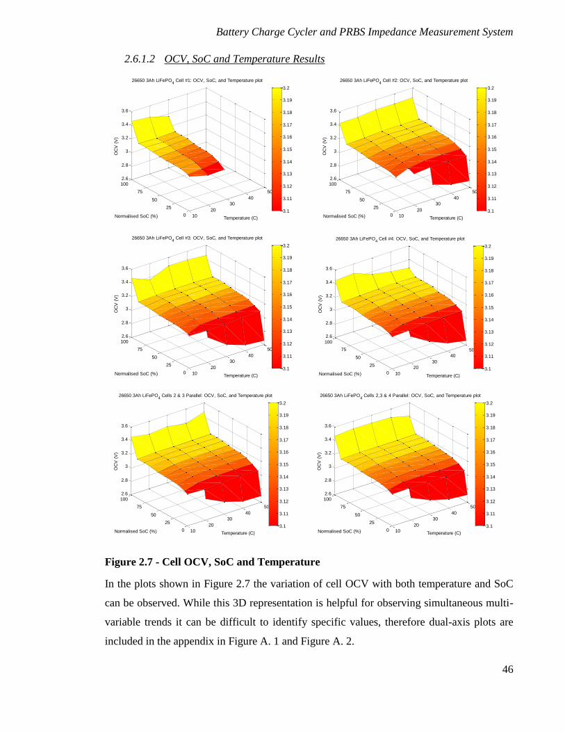
Battery Charge Cycler and PRBS Impedance Measurement System
46
2.6.1.2 OCV, SoC and Temperature Results
Figure 2.7 - Cell OCV, SoC and Temperature
In the plots shown in Figure 2.7 the variation of cell OCV with both temperature and SoC
can be observed. While this 3D representation is helpful for observing simultaneous multi-
variable trends it can be difficult to identify specific values, therefore dual-axis plots are
included in the appendix in Figure A. 1 and Figure A. 2.
10
20
30
40
50
0
25
50
75
1002.6
2.8
3
3.2
3.4
3.6
Temperature (C)
26650 3Ah LiFePO4 Cell #1: OCV, SoC, and Temperature plot
Normalised SoC (%)
OC
V (
V)
3.1
3.11
3.12
3.13
3.14
3.15
3.16
3.17
3.18
3.19
3.2
10
20
30
40
50
0
25
50
75
1002.6
2.8
3
3.2
3.4
3.6
Temperature (C)
26650 3Ah LiFePO4 Cell #2: OCV, SoC, and Temperature plot
Normalised SoC (%)
OC
V (
V)
3.1
3.11
3.12
3.13
3.14
3.15
3.16
3.17
3.18
3.19
3.2
10
20
30
40
50
0
25
50
75
1002.6
2.8
3
3.2
3.4
3.6
Temperature (C)
26650 3Ah LiFePO4 Cell #3: OCV, SoC, and Temperature plot
Normalised SoC (%)
OC
V (
V)
3.1
3.11
3.12
3.13
3.14
3.15
3.16
3.17
3.18
3.19
3.2
10
20
30
40
50
0
25
50
75
100
2.6
2.8
3
3.2
3.4
3.6
Temperature (C)
26650 3Ah LiFePO4 Cell #4: OCV, SoC, and Temperature plot
Normalised SoC (%)
OC
V (
V)
3.1
3.11
3.12
3.13
3.14
3.15
3.16
3.17
3.18
3.19
3.2
10
20
30
40
50
0
25
50
75
1002.6
2.8
3
3.2
3.4
3.6
Temperature (C)
26650 3Ah LiFePO4 Cells 2 & 3 Parallel: OCV, SoC, and Temperature plot
Normalised SoC (%)
OC
V (
V)
3.1
3.11
3.12
3.13
3.14
3.15
3.16
3.17
3.18
3.19
3.2
10
20
30
40
50
0
25
50
75
1002.6
2.8
3
3.2
3.4
3.6
Temperature (C)
26650 3Ah LiFePO4 Cells 2,3 & 4 Parallel: OCV, SoC, and Temperature plot
Normalised SoC (%)
OC
V (
V)
3.1
3.11
3.12
3.13
3.14
3.15
3.16
3.17
3.18
3.19
3.2
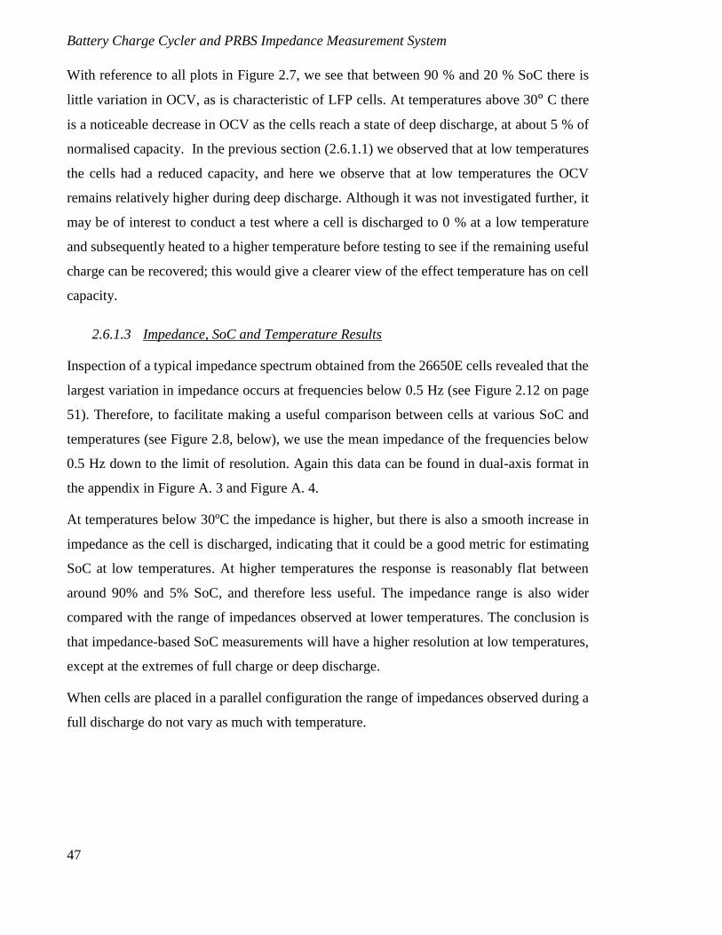
Battery Charge Cycler and PRBS Impedance Measurement System
47
With reference to all plots in Figure 2.7, we see that between 90 % and 20 % SoC there is
little variation in OCV, as is characteristic of LFP cells. At temperatures above 30ᵒ C there
is a noticeable decrease in OCV as the cells reach a state of deep discharge, at about 5 % of
normalised capacity. In the previous section (2.6.1.1) we observed that at low temperatures
the cells had a reduced capacity, and here we observe that at low temperatures the OCV
remains relatively higher during deep discharge. Although it was not investigated further, it
may be of interest to conduct a test where a cell is discharged to 0 % at a low temperature
and subsequently heated to a higher temperature before testing to see if the remaining useful
charge can be recovered; this would give a clearer view of the effect temperature has on cell
capacity.
2.6.1.3 Impedance, SoC and Temperature Results
Inspection of a typical impedance spectrum obtained from the 26650E cells revealed that the
largest variation in impedance occurs at frequencies below 0.5 Hz (see Figure 2.12 on page
51). Therefore, to facilitate making a useful comparison between cells at various SoC and
temperatures (see Figure 2.8, below), we use the mean impedance of the frequencies below
0.5 Hz down to the limit of resolution. Again this data can be found in dual-axis format in
the appendix in Figure A. 3 and Figure A. 4.
At temperatures below 30oC the impedance is higher, but there is also a smooth increase in
impedance as the cell is discharged, indicating that it could be a good metric for estimating
SoC at low temperatures. At higher temperatures the response is reasonably flat between
around 90% and 5% SoC, and therefore less useful. The impedance range is also wider
compared with the range of impedances observed at lower temperatures. The conclusion is
that impedance-based SoC measurements will have a higher resolution at low temperatures,
except at the extremes of full charge or deep discharge.
When cells are placed in a parallel configuration the range of impedances observed during a
full discharge do not vary as much with temperature.
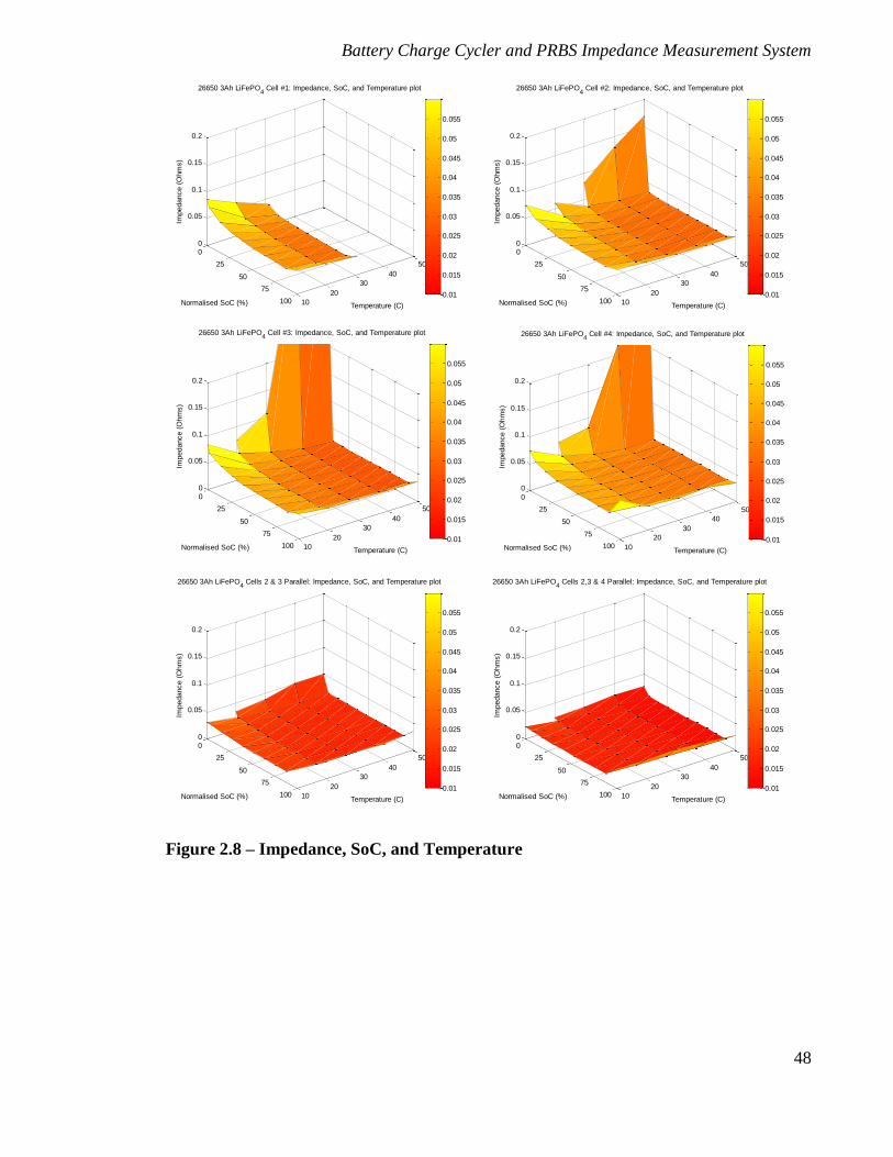
Battery Charge Cycler and PRBS Impedance Measurement System
48
Figure 2.8 – Impedance, SoC, and Temperature
10
20
30
40
50
0
25
50
75
100
0
0.05
0.1
0.15
0.2
Temperature (C)
26650 3Ah LiFePO4 Cell #1: Impedance, SoC, and Temperature plot
Normalised SoC (%)
Impedance (
Ohm
s)
0.01
0.015
0.02
0.025
0.03
0.035
0.04
0.045
0.05
0.055
10
20
30
40
50
0
25
50
75
100
0
0.05
0.1
0.15
0.2
Temperature (C)
26650 3Ah LiFePO4 Cell #2: Impedance, SoC, and Temperature plot
Normalised SoC (%)
Impedance (
Ohm
s)
0.01
0.015
0.02
0.025
0.03
0.035
0.04
0.045
0.05
0.055
10
20
30
40
50
0
25
50
75
100
0
0.05
0.1
0.15
0.2
Temperature (C)
26650 3Ah LiFePO4 Cell #3: Impedance, SoC, and Temperature plot
Normalised SoC (%)
Impedance (
Ohm
s)
0.01
0.015
0.02
0.025
0.03
0.035
0.04
0.045
0.05
0.055
10
20
30
40
50
0
25
50
75
100
0
0.05
0.1
0.15
0.2
Temperature (C)
26650 3Ah LiFePO4 Cell #4: Impedance, SoC, and Temperature plot
Normalised SoC (%)
Impedance (
Ohm
s)
0.01
0.015
0.02
0.025
0.03
0.035
0.04
0.045
0.05
0.055
10
20
30
40
50
0
25
50
75
100
0
0.05
0.1
0.15
0.2
Temperature (C)
26650 3Ah LiFePO4 Cells 2 & 3 Parallel: Impedance, SoC, and Temperature plot
Normalised SoC (%)
Impedance (
Ohm
s)
0.01
0.015
0.02
0.025
0.03
0.035
0.04
0.045
0.05
0.055
10
20
30
40
50
0
25
50
75
100
0
0.05
0.1
0.15
0.2
Temperature (C)
26650 3Ah LiFePO4 Cells 2,3 & 4 Parallel: Impedance, SoC, and Temperature plot
Normalised SoC (%)
Impedance (
Ohm
s)
0.01
0.015
0.02
0.025
0.03
0.035
0.04
0.045
0.05
0.055
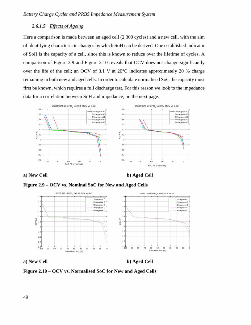
Battery Charge Cycler and PRBS Impedance Measurement System
49
2.6.1.5 Effects of Ageing
Here a comparison is made between an aged cell (2,300 cycles) and a new cell, with the aim
of identifying characteristic changes by which SoH can be derived. One established indicator
of SoH is the capacity of a cell, since this is known to reduce over the lifetime of cycles. A
comparison of Figure 2.9 and Figure 2.10 reveals that OCV does not change significantly
over the life of the cell; an OCV of 3.1 V at 20°C indicates approximately 20 % charge
remaining in both new and aged cells. In order to calculate normalised SoC the capacity must
first be known, which requires a full discharge test. For this reason we look to the impedance
data for a correlation between SoH and impedance, on the next page.
a) New Cell b) Aged Cell
Figure 2.9 – OCV vs. Nominal SoC for New and Aged Cells
a) New Cell b) Aged Cell
Figure 2.10 – OCV vs. Normalised SoC for New and Aged Cells
0204060801002.6
2.7
2.8
2.9
3
3.1
3.2
3.3
3.4
3.5
3.6
SoC (% of nominal)
OC
V (
V)
26650 3Ah LiFePO4 Cell #3: OCV vs SoC
10 degrees C
20 degrees C
30 degrees C
40 degrees C
50 degrees C
0204060801002.6
2.7
2.8
2.9
3
3.1
3.2
3.3
3.4
3.5
3.6
SoC (% of nominal)
OC
V (
V)
26650 3Ah LiFePO4 Cell #5: OCV vs SoC
10 degrees C
20 degrees C
30 degrees C
40 degrees C
50 degrees C
01020304050607080901002.6
2.7
2.8
2.9
3
3.1
3.2
3.3
3.4
3.5
3.6
Normalised SoC (%)
OC
V (
V)
26650 3Ah LiFePO4 Cell #3: OCV vs SoC
10 degrees C
20 degrees C
30 degrees C
40 degrees C
50 degrees C
01020304050607080901002.6
2.7
2.8
2.9
3
3.1
3.2
3.3
3.4
3.5
3.6
Normalised SoC (%)
OC
V (
V)
26650 3Ah LiFePO4 Cell #5: OCV vs SoC
10 degrees C
20 degrees C
30 degrees C
40 degrees C
50 degrees C
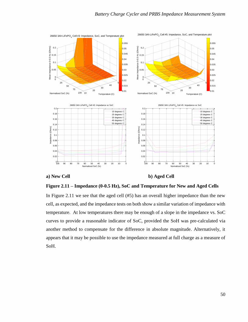
Battery Charge Cycler and PRBS Impedance Measurement System
50
a) New Cell b) Aged Cell
Figure 2.11 – Impedance (0-0.5 Hz), SoC and Temperature for New and Aged Cells
In Figure 2.11 we see that the aged cell (#5) has an overall higher impedance than the new
cell, as expected, and the impedance tests on both show a similar variation of impedance with
temperature. At low temperatures there may be enough of a slope in the impedance vs. SoC
curves to provide a reasonable indicator of SoC, provided the SoH was pre-calculated via
another method to compensate for the difference in absolute magnitude. Alternatively, it
appears that it may be possible to use the impedance measured at full charge as a measure of
SoH.
10
20
30
4050
0
25
50
75
100
0
0.05
0.1
0.15
0.2
Temperature (C)
26650 3Ah LiFePO4 Cell #3: Impedance, SoC, and Temperature plot
Normalised SoC (%)
Me
an
Im
pe
da
nce
0-0
.5 H
z (
Oh
ms)
0.01
0.015
0.02
0.025
0.03
0.035
0.04
0.045
0.05
0.055
10
20
3040
50
0
25
50
75
100
0
0.05
0.1
0.15
0.2
Temperature (C)
26650 3Ah LiFePO4 Cell #5: Impedance, SoC, and Temperature plot
Normalised SoC (%)
Me
an
Im
pe
da
nce
0-0
.5 H
z (
Oh
ms)
0.01
0.015
0.02
0.025
0.03
0.035
0.04
0.045
0.05
0.055
01020304050607080901000
0.02
0.04
0.06
0.08
0.1
0.12
0.14
0.16
0.18
0.2
Normalised SoC (%)
Impedance (
Ohm
s)
26650 3Ah LiFePO4 Cell #3: Impedance vs SoC
10 degrees C
20 degrees C
30 degrees C
40 degrees C
50 degrees C
01020304050607080901000
0.02
0.04
0.06
0.08
0.1
0.12
0.14
0.16
0.18
0.2
Normalised SoC (%)
Impedance (
Ohm
s)
26650 3Ah LiFePO4 Cell #5: Impedance vs SoC
10 degrees C
20 degrees C
30 degrees C
40 degrees C
50 degrees C
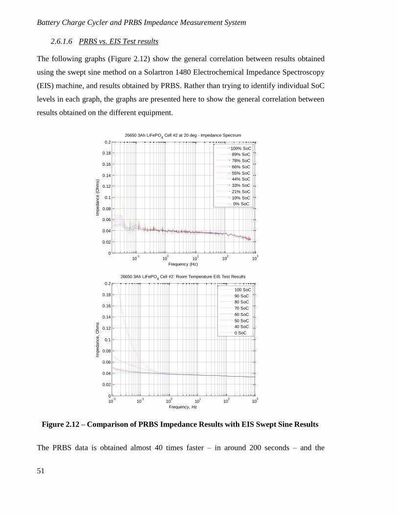
Battery Charge Cycler and PRBS Impedance Measurement System
51
2.6.1.6 PRBS vs. EIS Test results
The following graphs (Figure 2.12) show the general correlation between results obtained
using the swept sine method on a Solartron 1480 Electrochemical Impedance Spectroscopy
(EIS) machine, and results obtained by PRBS. Rather than trying to identify individual SoC
levels in each graph, the graphs are presented here to show the general correlation between
results obtained on the different equipment.
The PRBS data is obtained almost 40 times faster – in around 200 seconds – and the
Figure 2.12 – Comparison of PRBS Impedance Results with EIS Swept Sine Results
10-1
100
101
102
103
0
0.02
0.04
0.06
0.08
0.1
0.12
0.14
0.16
0.18
0.2
Frequency (Hz)
Impedance (
Ohm
s)
26650 3Ah LiFePO4 Cell #2 at 20 deg - Impedance Spectrum
100% SoC
89% SoC
78% SoC
66% SoC
55% SoC
44% SoC
33% SoC
21% SoC
10% SoC
0% SoC
10-2
10-1
100
101
102
103
0
0.02
0.04
0.06
0.08
0.1
0.12
0.14
0.16
0.18
0.2
Frequency, Hz
Impedance,
Ohm
s
26650 3Ah LiFePO4 Cell #2: Room Temperature EIS Test Results
100 SoC
90 SoC
80 SoC
70 SoC
60 SoC
50 SoC
40 SoC
0 SoC
Battery Charge Cycler and PRBS Impedance Measurement System
52
equipment cost is a fraction of the EIS test equipment cost. A comparison of the results show
good correlation apart from the 100 % SoC test, but this can be explained by different
relaxation times prior to beginning the tests; the EIS test was started immediately after a full
charge, with no voltage relaxation period preceding it.
Apparent in Figure 2.12, as mentioned previously, is that at frequencies above 0.5 Hz both
tests reveal little difference in impedance as the SoC changes. The PRBS results diverge from
the EIS measurements at frequencies above around 100 Hz, and reasons for this are proposed
in section 2.7. Otherwise, the results show good correlation.
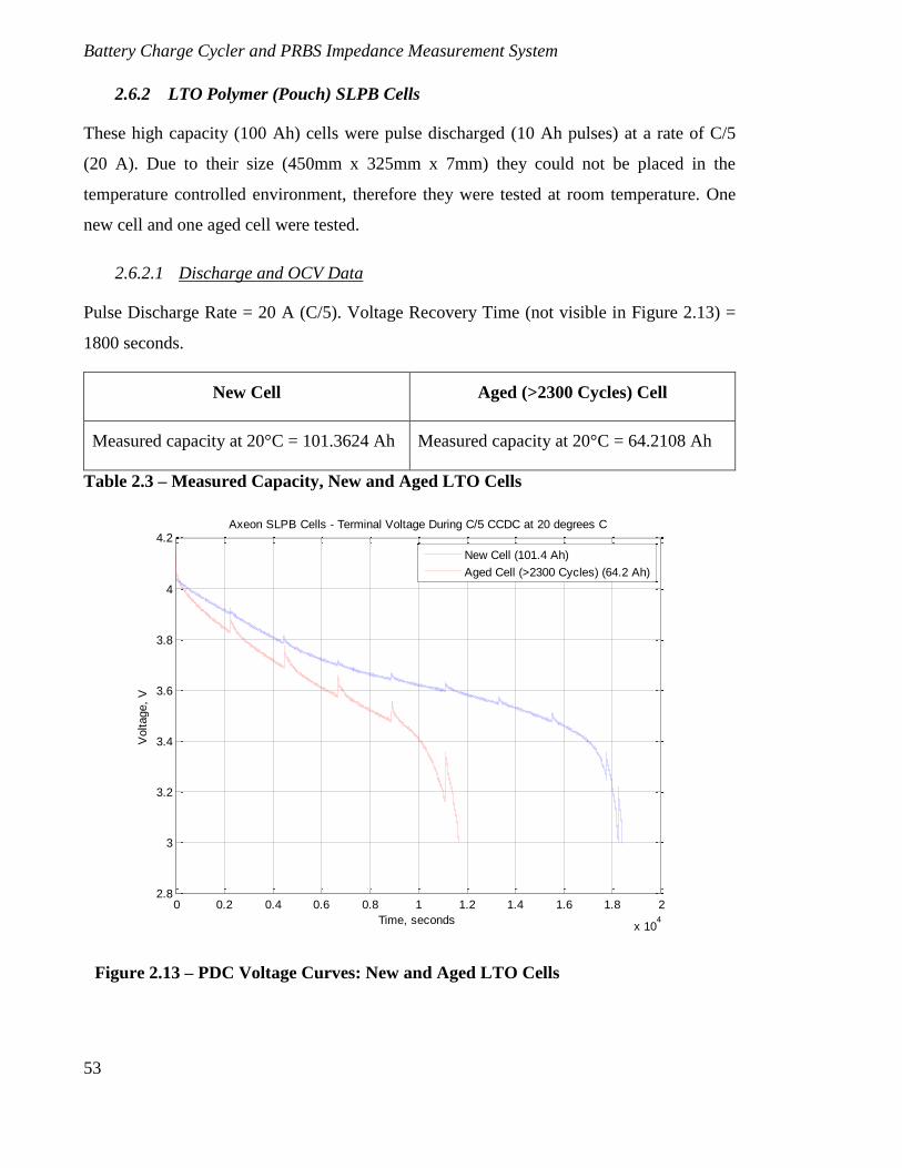
Battery Charge Cycler and PRBS Impedance Measurement System
53
2.6.2 LTO Polymer (Pouch) SLPB Cells
These high capacity (100 Ah) cells were pulse discharged (10 Ah pulses) at a rate of C/5
(20 A). Due to their size (450mm x 325mm x 7mm) they could not be placed in the
temperature controlled environment, therefore they were tested at room temperature. One
new cell and one aged cell were tested.
2.6.2.1 Discharge and OCV Data
Pulse Discharge Rate = 20 A (C/5). Voltage Recovery Time (not visible in Figure 2.13) =
1800 seconds.
New Cell Aged (>2300 Cycles) Cell
Measured capacity at 20°C = 101.3624 Ah Measured capacity at 20°C = 64.2108 Ah
Table 2.3 – Measured Capacity, New and Aged LTO Cells
Figure 2.13 – PDC Voltage Curves: New and Aged LTO Cells
0 0.2 0.4 0.6 0.8 1 1.2 1.4 1.6 1.8 2
x 104
2.8
3
3.2
3.4
3.6
3.8
4
4.2Axeon SLPB Cells - Terminal Voltage During C/5 CCDC at 20 degrees C
Time, seconds
Voltage,
V
New Cell (101.4 Ah)
Aged Cell (>2300 Cycles) (64.2 Ah)
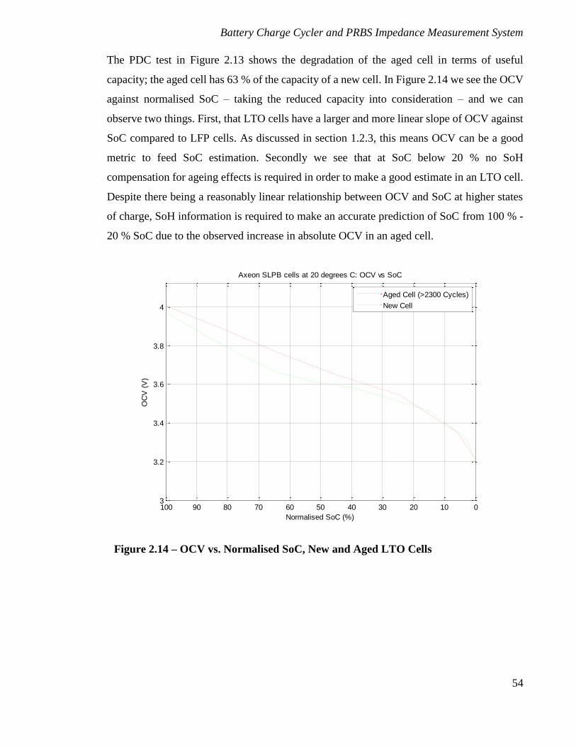
Battery Charge Cycler and PRBS Impedance Measurement System
54
The PDC test in Figure 2.13 shows the degradation of the aged cell in terms of useful
capacity; the aged cell has 63 % of the capacity of a new cell. In Figure 2.14 we see the OCV
against normalised SoC – taking the reduced capacity into consideration – and we can
observe two things. First, that LTO cells have a larger and more linear slope of OCV against
SoC compared to LFP cells. As discussed in section 1.2.3, this means OCV can be a good
metric to feed SoC estimation. Secondly we see that at SoC below 20 % no SoH
compensation for ageing effects is required in order to make a good estimate in an LTO cell.
Despite there being a reasonably linear relationship between OCV and SoC at higher states
of charge, SoH information is required to make an accurate prediction of SoC from 100 % -
20 % SoC due to the observed increase in absolute OCV in an aged cell.
Figure 2.14 – OCV vs. Normalised SoC, New and Aged LTO Cells
01020304050607080901003
3.2
3.4
3.6
3.8
4
Normalised SoC (%)
OC
V (
V)
Axeon SLPB cells at 20 degrees C: OCV vs SoC
Aged Cell (>2300 Cycles)
New Cell
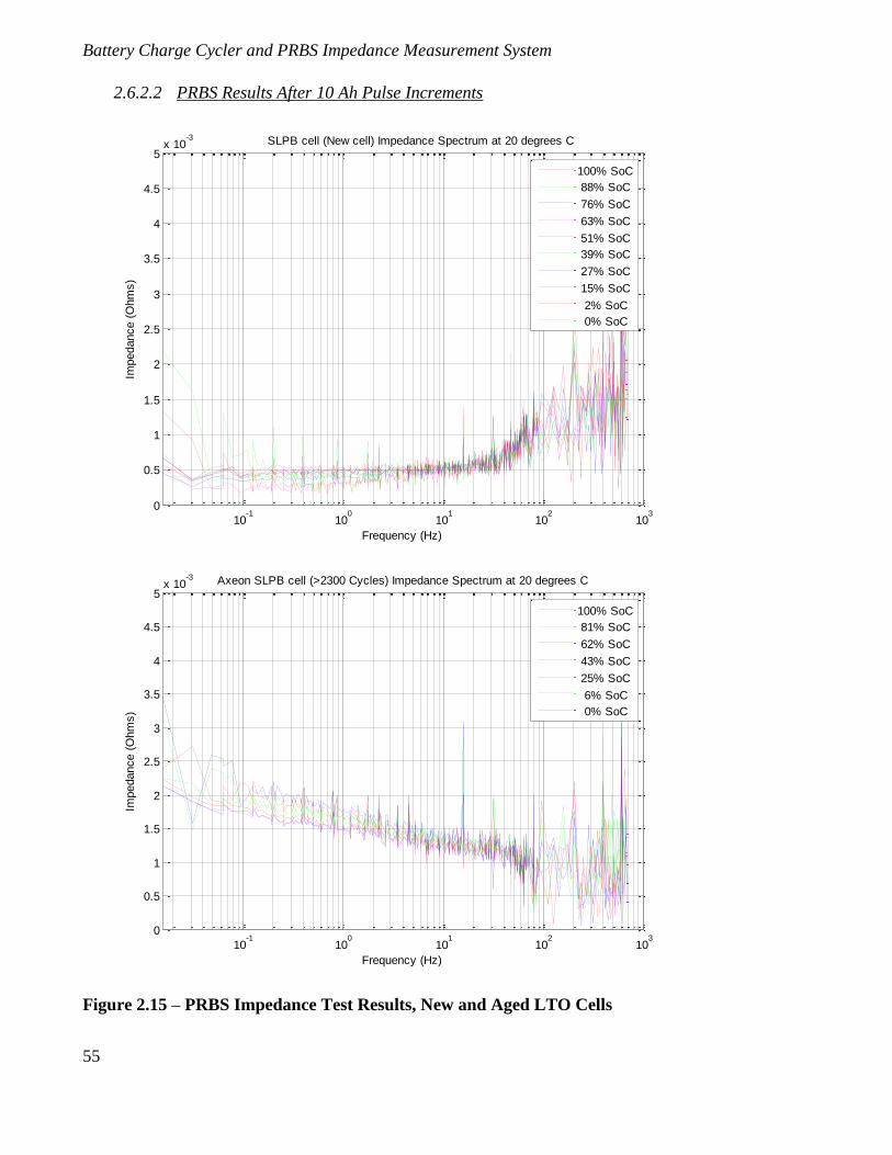
Battery Charge Cycler and PRBS Impedance Measurement System
55
2.6.2.2 PRBS Results After 10 Ah Pulse Increments
Figure 2.15 – PRBS Impedance Test Results, New and Aged LTO Cells
10-1
100
101
102
103
0
0.5
1
1.5
2
2.5
3
3.5
4
4.5
5x 10
-3
Frequency (Hz)
Impedance (
Ohm
s)
Axeon SLPB cell (New cell) Impedance Spectrum at 20 degrees C
100% SoC
88% SoC
76% SoC
63% SoC
51% SoC
39% SoC
27% SoC
15% SoC
2% SoC
0% SoC
10-1
100
101
102
103
0
0.5
1
1.5
2
2.5
3
3.5
4
4.5
5x 10
-3
Frequency (Hz)
Impedance (
Ohm
s)
Axeon SLPB cell (>2300 Cycles) Impedance Spectrum at 20 degrees C
100% SoC
81% SoC
62% SoC
43% SoC
25% SoC
6% SoC
0% SoC
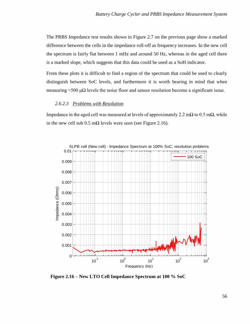
Battery Charge Cycler and PRBS Impedance Measurement System
56
The PRBS Impedance test results shown in Figure 2.7 on the previous page show a marked
difference between the cells in the impedance roll-off as frequency increases. In the new cell
the spectrum is fairly flat between 1 mHz and around 50 Hz, whereas in the aged cell there
is a marked slope, which suggests that this data could be used as a SoH indicator.
From these plots it is difficult to find a region of the spectrum that could be used to clearly
distinguish between SoC levels, and furthermore it is worth bearing in mind that when
measuring ≈500 μΩ levels the noise floor and sensor resolution become a significant issue.
2.6.2.3 Problems with Resolution
Impedance in the aged cell was measured at levels of approximately 2.2 mΩ to 0.5 mΩ, while
in the new cell sub 0.5 mΩ levels were seen (see Figure 2.16).
Figure 2.16 – New LTO Cell Impedance Spectrum at 100 % SoC
10-1
100
101
102
103
0
0.001
0.002
0.003
0.004
0.005
0.006
0.007
0.008
0.009
0.01
Frequency (Hz)
Impedance (
Ohm
s)
SLPB cell (New cell) - Impedance Spectrum at 100% SoC; resolution problems
100 SoC
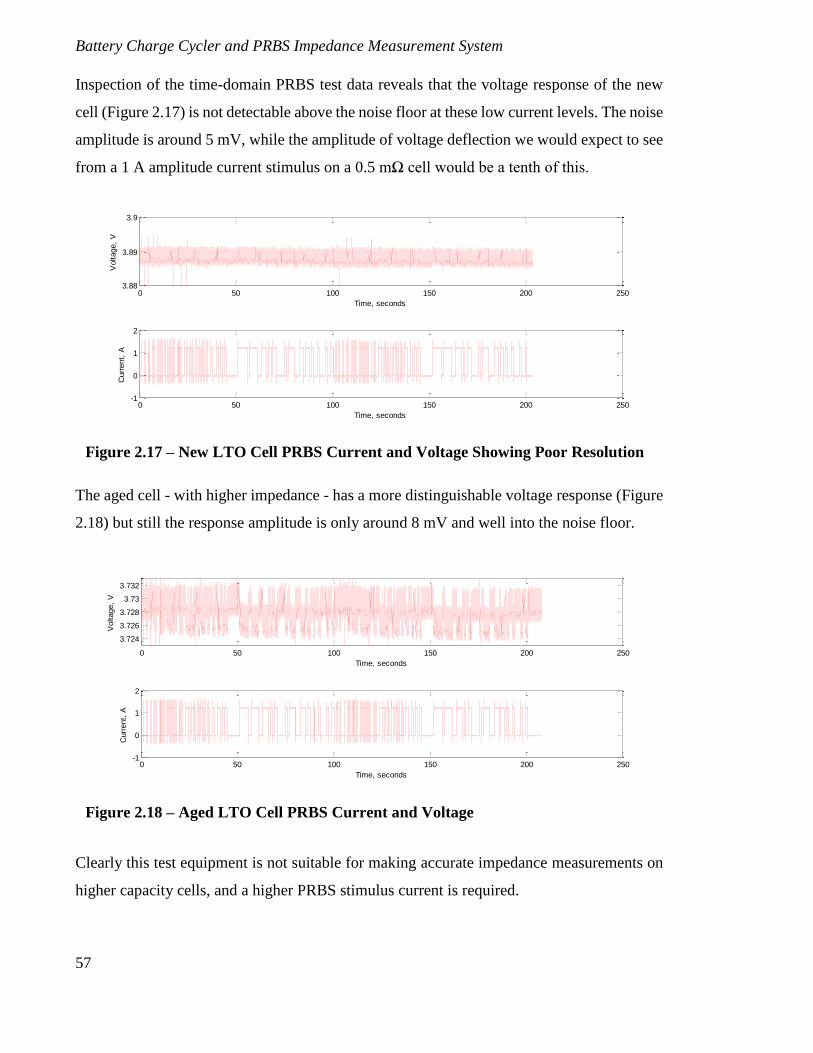
Battery Charge Cycler and PRBS Impedance Measurement System
57
Inspection of the time-domain PRBS test data reveals that the voltage response of the new
cell (Figure 2.17) is not detectable above the noise floor at these low current levels. The noise
amplitude is around 5 mV, while the amplitude of voltage deflection we would expect to see
from a 1 A amplitude current stimulus on a 0.5 mΩ cell would be a tenth of this.
The aged cell - with higher impedance - has a more distinguishable voltage response (Figure
2.18) but still the response amplitude is only around 8 mV and well into the noise floor.
Clearly this test equipment is not suitable for making accurate impedance measurements on
higher capacity cells, and a higher PRBS stimulus current is required.
Figure 2.17 – New LTO Cell PRBS Current and Voltage Showing Poor Resolution
0 50 100 150 200 2503.6
3.8
4
Voltage,
V
Time, seconds
0 50 100 150 200 250-2
0
2
Curr
ent,
A
0 50 100 150 200 2503.88
3.89
3.9
Time, seconds
Voltage,
V
0 50 100 150 200 250-1
0
1
2
Time, seconds
Curr
ent,
A
Figure 2.18 – Aged LTO Cell PRBS Current and Voltage
0 50 100 150 200 2503.65
3.7
3.75
3.8
Voltage,
V
Time, seconds
0 50 100 150 200 250-1
0
1
2
Curr
ent,
A
0 50 100 150 200 250
3.724
3.726
3.728
3.73
3.732
Time, seconds
Voltage,
V
0 50 100 150 200 250-1
0
1
2
Time, seconds
Curr
ent,
A
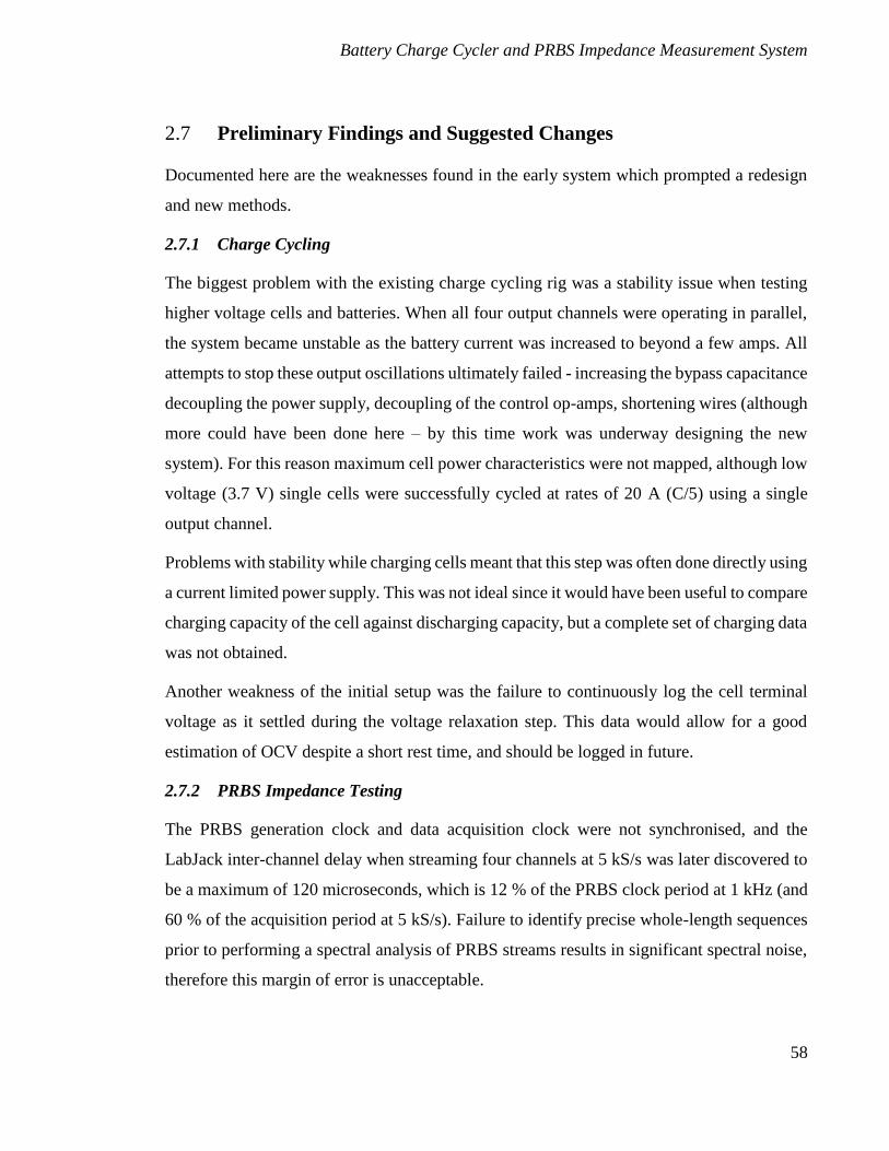
Battery Charge Cycler and PRBS Impedance Measurement System
58
2.7 Preliminary Findings and Suggested Changes
Documented here are the weaknesses found in the early system which prompted a redesign
and new methods.
2.7.1 Charge Cycling
The biggest problem with the existing charge cycling rig was a stability issue when testing
higher voltage cells and batteries. When all four output channels were operating in parallel,
the system became unstable as the battery current was increased to beyond a few amps. All
attempts to stop these output oscillations ultimately failed - increasing the bypass capacitance
decoupling the power supply, decoupling of the control op-amps, shortening wires (although
more could have been done here – by this time work was underway designing the new
system). For this reason maximum cell power characteristics were not mapped, although low
voltage (3.7 V) single cells were successfully cycled at rates of 20 A (C/5) using a single
output channel.
Problems with stability while charging cells meant that this step was often done directly using
a current limited power supply. This was not ideal since it would have been useful to compare
charging capacity of the cell against discharging capacity, but a complete set of charging data
was not obtained.
Another weakness of the initial setup was the failure to continuously log the cell terminal
voltage as it settled during the voltage relaxation step. This data would allow for a good
estimation of OCV despite a short rest time, and should be logged in future.
2.7.2 PRBS Impedance Testing
The PRBS generation clock and data acquisition clock were not synchronised, and the
LabJack inter-channel delay when streaming four channels at 5 kS/s was later discovered to
be a maximum of 120 microseconds, which is 12 % of the PRBS clock period at 1 kHz (and
60 % of the acquisition period at 5 kS/s). Failure to identify precise whole-length sequences
prior to performing a spectral analysis of PRBS streams results in significant spectral noise,
therefore this margin of error is unacceptable.
Battery Charge Cycler and PRBS Impedance Measurement System
59
Further, the PRBS generation clock signal itself was not hardware timed. The binary
sequence was read in a software ‘for’ loop, reading each bit from a variable stored in memory,
and an ‘if… else’ statement decided whether to make the digital output pin high or low. An
attempt was made to mitigate the errors introduced as a result of the use of software timing
by taking oscilloscope measurements of single PRBS bit periods to confirm the actual clock
rate for correction purposes. However, another source of timing error may be introduced
when performing ‘if… else’ statements within a software loop, due to the two outcomes
(if/else) having different execution time after the code is compiled. Ultimately these bring
uncertainties into the work which could be avoided with the use of hardware timing and
synchronised generation and acquisition clocks.
14-bit resolution was found not to be sufficient to accurately measure the response voltage
when testing large capacity cells (50 Ah and above) at low (1 A) PRBS currents. One solution
is to increase both the stimulation current and the measuring resolution (use 16-bits
resolution, and increase current to +/- 5 A). It is also prudent to make bipolar stimulus a
requirement, so that the overall state of charge is not affected during the impedance test.
System Identification requires that the system state does not change for the duration of the
test.
Still considering resolution, we must ask ourselves about the final application. If PRBS
impedance measurement is to be embedded in say an EV BMS, then very low impedance
levels such as those seen in the LTO cells require sensitive measurement instruments. These
are not commonly available in very high cell-count battery packs, where 5 mV resolution is
considered to be good [52].
Finally, the PRBS frequencies chosen were based on values inherited from previous work in
the group. It was later confirmed that those frequencies were in fact chosen to suit a particular
microcontroller’s counter divisions. With this information, a more logical choice in a new
system would be to choose roughly logarithmic frequency intervals, such as 1, 2, 5, 10 and
so on, as these produce an even spread of data points on a logarithmic frequency plot.
These findings form the basis for the development of the system described in the next chapter.
60
Chapter 3: Charge Cycler/Impedance Analyser Specification and
Design
3.1 Objectives
As discussed in the previous section, weaknesses in the early design prompted ideas for
improvement which could be met with a new design. Previously built hardware was limited
in three ways which were to be addressed:
1. Unipolar current. During a system identification test it is important that the system
being measured does not change state over the duration of the test; that is, its final
state (e.g. SOC of a battery) must be the same as its initial state. Some low frequency
aliasing effects in impedance spectra gathered from the unipolar PRBS rig can be
explained by the fact that during the course of the system identification tests the state
of the system was in fact changing at a very low rate. This unwanted effect can be
avoided by using bipolar stimulus that has no net effect on charge over the duration
of the test.
2. Amplitude. The previous hardware was limited to 1.5 A pulses which is not a high
enough current stimulus to cause sufficient voltage deflection in larger capacity
(> 20 Ah) cells. Upgrading from 14 to 16-bit data acquisition went some way to
improving measurements, but the capability to drive larger currents would provide
better results (improved SNR).
3. Timing. The previous hardware relied on software timing to clock the PRBS stream,
and asynchronous hardware timed data-acquisition. The new design uses hardware
timing for both PRBS generation and acquisition and synchronises data acquisition
with the stimulus pulse edges.
3.2 Hardware Design and Construction
3.2.1 Target Specification
A transconductance amplifier was required that could perform charge cycling and PRBS
stimulus/response measurements on a variety of battery cells and single port networks.
Table 3.1 lists the proposed minimum requirements.
Charge Cycler/Impedance Analyser Specification and Design
61
3.2.2 Design Steps
3.2.2.1 Overview
In order to provide test equipment of high reliability and robustness, some aspects of the
design involved increasing the target specification to allow a comfortable overhead during
longer test cycles. Reliability and flexibility of the equipment was an important factor,
therefore the design was based on a continuous current rating of 200% (+/- 10 A) with 125%
of rated Device Under Test (DUT) Voltage (7.4 V max). Furthermore the DUT voltage range
was extended down to 0 V in order that passive networks could be tested, which would aid
calibration of the rig.
The overall topology (full schematic in the appendix) is based around a BJT push-pull output
stage powered from a bipolar DC link. A link voltage of +/- 12 V was chosen for convenience.
There is a Voltage Amplification Stage (VAS) which is loaded by a small current source and
a pre-driver bias circuit to maintain class B amplification, thus minimising crossover
distortion with minimal quiescent current. Control of the output current is achieved using a
reference voltage to drive the VAS via a differential amplifier.
DUT Voltage Range 1.5 V – 6 V
DUT Current Range ± 5 A
Acquisition Sample Rate 10 kHz desirable, 5kHz acceptable
NI USB-DAQ 6211 Synchronised simultaneous V and I measurement
ADCs
Synchronised sample and PRBS clock
System Tests Prove on an RC network, charge and discharge at
rated current, and obtain impedance spectrum.
Validate results against those from a spectrum
analyser.
Then cycle a battery and do a PRBS impedance
analysis.
Table 3.1 – Minimum Requirements
Charge Cycler/Impedance Analyser Specification and Design
62
3.2.2.2 Output Stage Devices
Transistors available in the local Electronic Stores were chosen for the design so that in case
of failure minimum downtime would be suffered. Figure 3.1 shows the Safe Operating Area
(SOA) of the TIP3055 and the complementary pnp type TIP2955. The design criteria of
discharging a 7.4 V battery at 10 A into a -12 V link places the required operating area on a
vertical line denoted by Vce = 19.4 V, which corresponds to a maximum current of roughly
4 A, capped by the thermal limit of the low-side devices. A minimum of three devices in
parallel are required therefore, to meet the 10 A current requirement, and four were chosen
in the design to provide suitable de-rating.
Small emitter degeneration resistors are fitted to each output device so that current is shared
equally between devices. Due to the negative temperature coefficient of BJTs, if one device
heats more than another this leads to an increase in current through that device; the 0.1 Ω
emitter degeneration resistor will compensate for this and prevent thermal runaway by
reducing the VCE across the device and thus a dynamic equilibrium is maintained between all
parallel devices.
Figure 3.1 – TIP3055/2955 BJT Safe Operating Area, single device
Charge Cycler/Impedance Analyser Specification and Design
63
3.2.2.3 Heatsink Requirements
The heatsink requirements were calculated using the same worst-case calculations as for the
output devices, see Figure 3.2.
The design assumption is that each output device will be expected to dissipate a maximum
of 50 W continuously. With reference to Figure 3.3 the thermal resistance between junction
and case of these devices is 1.4° C/W, while the thermal pads used add a further 0.425° C/W.
This means that the junction of each device will rise 92° C above the surface temperature of
the heatsink under maximum load conditions.
The absolute maximum allowable junction temperature (Tjunc) is 150° C. A good de-rating
factor might be 0.8, making the maximum allowable Tjunc = 120° C. However given that Tjunc
will always be 92° C above the heatsink surface temperature (Tsurf) this would require that
Tsurf not be allowed to exceed 30° C; this would require a heatsink with heatsink-to-ambient
thermal resistance of 0.019° C/W. This sort of heatsink requirement would need an exotic
Worst Case Low-Side Dissipation (one device of four is shown):
10 A continuous discharge of a 7.4 V DUT (2.5 A per low-side device)
Power dissipation = 50 W per device (200 W total).
Figure 3.2 – Output Stage Maximum Load
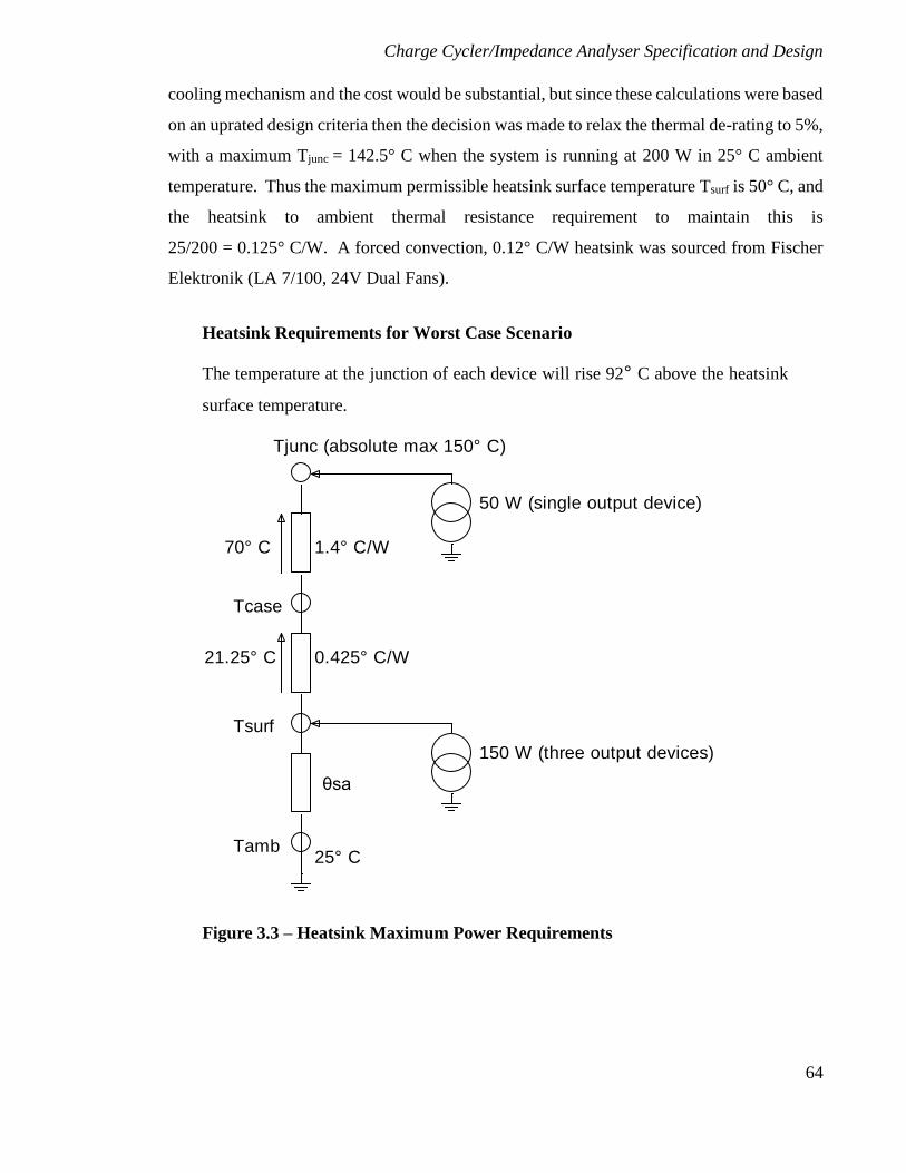
Charge Cycler/Impedance Analyser Specification and Design
64
cooling mechanism and the cost would be substantial, but since these calculations were based
on an uprated design criteria then the decision was made to relax the thermal de-rating to 5%,
with a maximum Tjunc = 142.5° C when the system is running at 200 W in 25° C ambient
temperature. Thus the maximum permissible heatsink surface temperature Tsurf is 50° C, and
the heatsink to ambient thermal resistance requirement to maintain this is
25/200 = 0.125° C/W. A forced convection, 0.12° C/W heatsink was sourced from Fischer
Elektronik (LA 7/100, 24V Dual Fans).
Heatsink Requirements for Worst Case Scenario
The temperature at the junction of each device will rise 92° C above the heatsink
surface temperature.
Figure 3.3 – Heatsink Maximum Power Requirements
25° C
Tcase
Tsurf
Tamb
21.25° C
1.4° C/W
0.425° C/W
θsa
50 W (single output device)
150 W (three output devices)
70° C
Tjunc (absolute max 150° C)
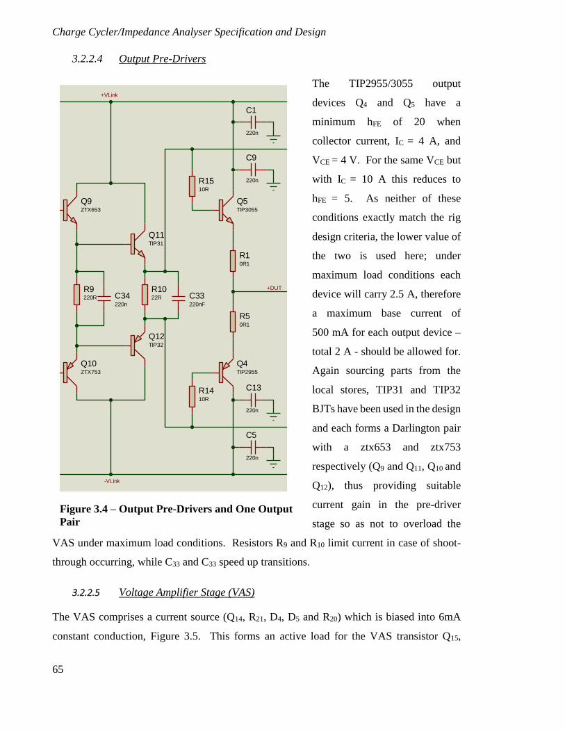
Charge Cycler/Impedance Analyser Specification and Design
65
3.2.2.4 Output Pre-Drivers
The TIP2955/3055 output
devices Q4 and Q5 have a
minimum hFE of 20 when
collector current, IC = 4 A, and
VCE = 4 V. For the same VCE but
with IC = 10 A this reduces to
hFE = 5. As neither of these
conditions exactly match the rig
design criteria, the lower value of
the two is used here; under
maximum load conditions each
device will carry 2.5 A, therefore
a maximum base current of
500 mA for each output device –
total 2 A - should be allowed for.
Again sourcing parts from the
local stores, TIP31 and TIP32
BJTs have been used in the design
and each forms a Darlington pair
with a ztx653 and ztx753
respectively (Q9 and Q11, Q10 and
Q12), thus providing suitable
current gain in the pre-driver
stage so as not to overload the
VAS under maximum load conditions. Resistors R9 and R10 limit current in case of shoot-
through occurring, while C33 and C33 speed up transitions.
3.2.2.5 Voltage Amplifier Stage (VAS)
The VAS comprises a current source (Q14, R21, D4, D5 and R20) which is biased into 6mA
constant conduction, Figure 3.5. This forms an active load for the VAS transistor Q15,
Figure 3.4 – Output Pre-Drivers and One Output
Pair
Q4TIP2955
Q9ZTX653
Q10ZTX753
Q11TIP31
Q12TIP32
R1022R
C1
220n
C5
220n
Q5TIP3055
R10R1
R50R1
R9220R
R1410R
R1510R
C9
220n
C13
220n
C33220nF
C34220n
-VLink
+VLink
+DUT
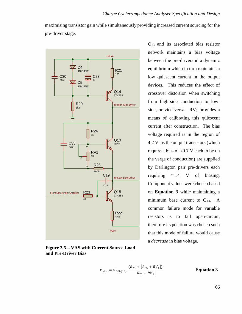
Charge Cycler/Impedance Analyser Specification and Design
66
maximising transistor gain while simultaneously providing increased current sourcing for the
pre-driver stage.
Q13 and its associated bias resistor
network maintains a bias voltage
between the pre-drivers in a dynamic
equilibrium which in turn maintains a
low quiescent current in the output
devices. This reduces the effect of
crossover distortion when switching
from high-side conduction to low-
side, or vice versa. RV1 provides a
means of calibrating this quiescent
current after construction. The bias
voltage required is in the region of
4.2 V, as the output transistors (which
require a bias of ≈0.7 V each to be on
the verge of conduction) are supplied
by Darlington pair pre-drivers each
requiring ≈1.4 V of biasing.
Component values were chosen based
on Equation 3 while maintaining a
minimum base current to Q13. A
common failure mode for variable
resistors is to fail open-circuit,
therefore its position was chosen such
that this mode of failure would cause
a decrease in bias voltage.
𝑉𝑏𝑖𝑎𝑠 = 𝑉𝐶𝐸(𝑄13).(𝑅24 + [𝑅25 + 𝑅𝑉1])
[𝑅25 + 𝑅𝑉1] Equation 3
Figure 3.5 – VAS with Current Source Load
and Pre-Driver Bias
Q14ZTX753
R203k3
R21120
Q15ZTX653
R2247R
R23
1k
R243k
R25
200R
13
2
RV11K
Q13TIP31
C231u
C30220n
C3522nF
C19
47pF
D41N4148W
D51N4148W
-VLink
+VLink
To High-Side Driver
To Low-Side Driver
From Differential Amplifier
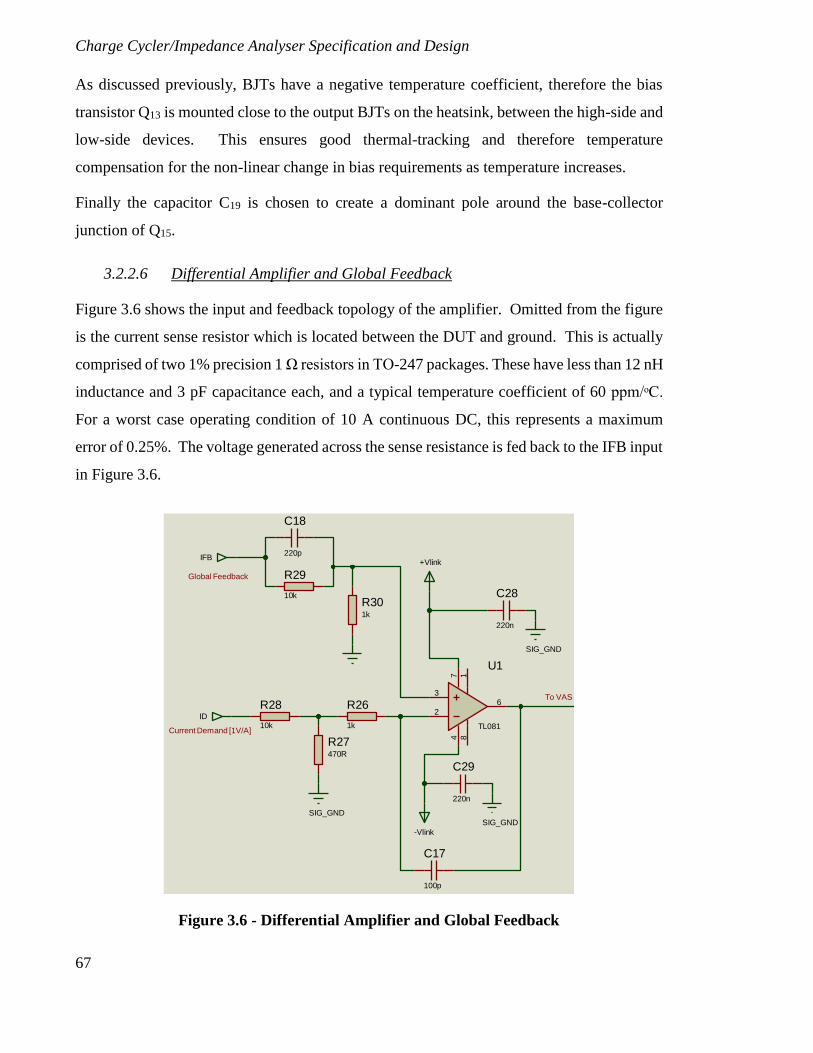
Charge Cycler/Impedance Analyser Specification and Design
67
As discussed previously, BJTs have a negative temperature coefficient, therefore the bias
transistor Q13 is mounted close to the output BJTs on the heatsink, between the high-side and
low-side devices. This ensures good thermal-tracking and therefore temperature
compensation for the non-linear change in bias requirements as temperature increases.
Finally the capacitor C19 is chosen to create a dominant pole around the base-collector
junction of Q15.
3.2.2.6 Differential Amplifier and Global Feedback
Figure 3.6 shows the input and feedback topology of the amplifier. Omitted from the figure
is the current sense resistor which is located between the DUT and ground. This is actually
comprised of two 1% precision 1 Ω resistors in TO-247 packages. These have less than 12 nH
inductance and 3 pF capacitance each, and a typical temperature coefficient of 60 ppm/ᵒC.
For a worst case operating condition of 10 A continuous DC, this represents a maximum
error of 0.25%. The voltage generated across the sense resistance is fed back to the IFB input
in Figure 3.6.
Figure 3.6 - Differential Amplifier and Global Feedback
3
2
6
74 8
1
U1
TL081
C17
100p
R26
1k
R27470R
SIG_GND
R28
10kID
R29
10k
C18
220p
R301k
IFB
C28
220n
C29
220n
SIG_GND
SIG_GND
+Vlink
-Vlink
Global Feedback
Current Demand [1V/A]
To VAS
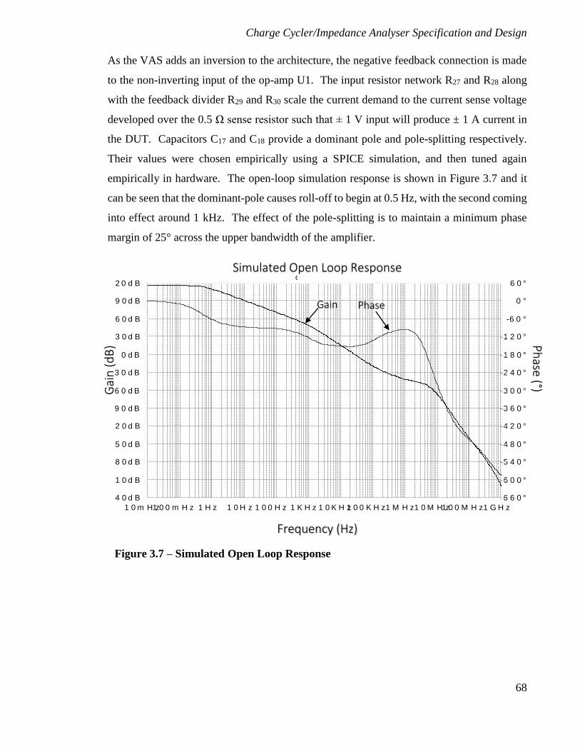
Charge Cycler/Impedance Analyser Specification and Design
68
As the VAS adds an inversion to the architecture, the negative feedback connection is made
to the non-inverting input of the op-amp U1. The input resistor network R27 and R28 along
with the feedback divider R29 and R30 scale the current demand to the current sense voltage
developed over the 0.5 Ω sense resistor such that ± 1 V input will produce ± 1 A current in
the DUT. Capacitors C17 and C18 provide a dominant pole and pole-splitting respectively.
Their values were chosen empirically using a SPICE simulation, and then tuned again
empirically in hardware. The open-loop simulation response is shown in Figure 3.7 and it
can be seen that the dominant-pole causes roll-off to begin at 0.5 Hz, with the second coming
into effect around 1 kHz. The effect of the pole-splitting is to maintain a minimum phase
margin of 25° across the upper bandwidth of the amplifier.
Figure 3.7 – Simulated Open Loop Response
1 0 m H z1 0 0 m H z 1 H z 1 0 H z 1 0 0 H z 1 K H z 1 0 K H z1 0 0 K H z1 M H z1 0 M H z1 0 0 M H z1 G H z
-2 4 0 d B
-2 1 0 d B
-1 8 0 d B
-1 5 0 d B
-1 2 0 d B
-9 0 d B
-6 0 d B
-3 0 d B
0 d B
3 0 d B
6 0 d B
9 0 d B
1 2 0 d B
-6 6 0 °
-6 0 0 °
-5 4 0 °
-4 8 0 °
-4 2 0 °
-3 6 0 °
-3 0 0 °
-2 4 0 °
-1 8 0 °
-1 2 0 °
-6 0 °
0 °
6 0 ° o p e n L o o p ( )
Gai
n (
dB
) Ph
ase (°)
Frequency (Hz)
Simulated Open Loop Response
Gain Phase
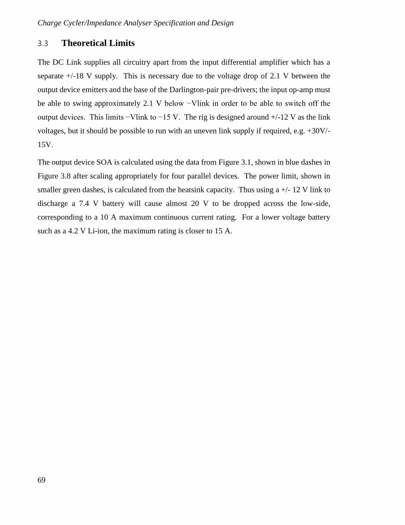
Charge Cycler/Impedance Analyser Specification and Design
69
3.3 Theoretical Limits
The DC Link supplies all circuitry apart from the input differential amplifier which has a
separate +/-18 V supply. This is necessary due to the voltage drop of 2.1 V between the
output device emitters and the base of the Darlington-pair pre-drivers; the input op-amp must
be able to swing approximately 2.1 V below −Vlink in order to be able to switch off the
output devices. This limits −Vlink to −15 V. The rig is designed around +/-12 V as the link
voltages, but it should be possible to run with an uneven link supply if required, e.g. +30V/-
15V.
The output device SOA is calculated using the data from Figure 3.1, shown in blue dashes in
Figure 3.8 after scaling appropriately for four parallel devices. The power limit, shown in
smaller green dashes, is calculated from the heatsink capacity. Thus using a +/- 12 V link to
discharge a 7.4 V battery will cause almost 20 V to be dropped across the low-side,
corresponding to a 10 A maximum continuous current rating. For a lower voltage battery
such as a 4.2 V Li-ion, the maximum rating is closer to 15 A.
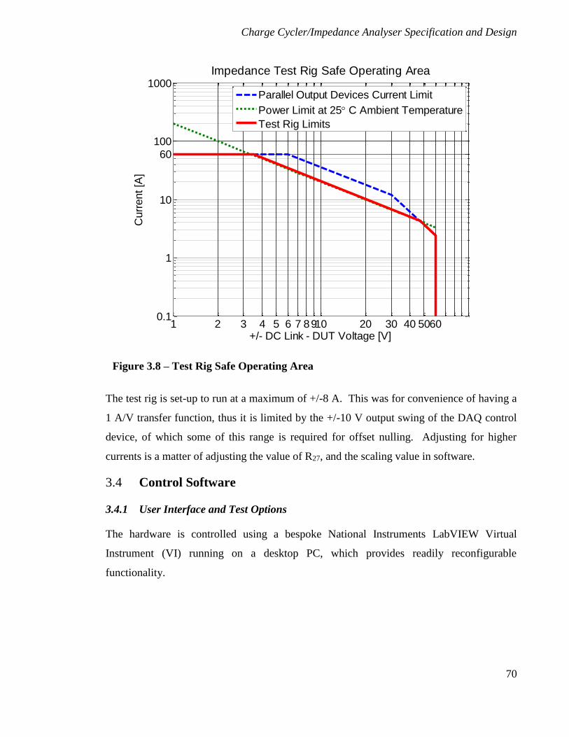
Charge Cycler/Impedance Analyser Specification and Design
70
The test rig is set-up to run at a maximum of +/-8 A. This was for convenience of having a
1 A/V transfer function, thus it is limited by the +/-10 V output swing of the DAQ control
device, of which some of this range is required for offset nulling. Adjusting for higher
currents is a matter of adjusting the value of R27, and the scaling value in software.
3.4 Control Software
3.4.1 User Interface and Test Options
The hardware is controlled using a bespoke National Instruments LabVIEW Virtual
Instrument (VI) running on a desktop PC, which provides readily reconfigurable
functionality.
Figure 3.8 – Test Rig Safe Operating Area
1 2 3 4 5 6 7 8910 20 30 40 50600.1
1
10
60
100
1000
+/- DC Link - DUT Voltage [V]
Curr
ent [A
]
Impedance Test Rig Safe Operating Area
Parallel Output Devices Current Limit
Power Limit at 25 C Ambient Temperature
Test Rig Limits
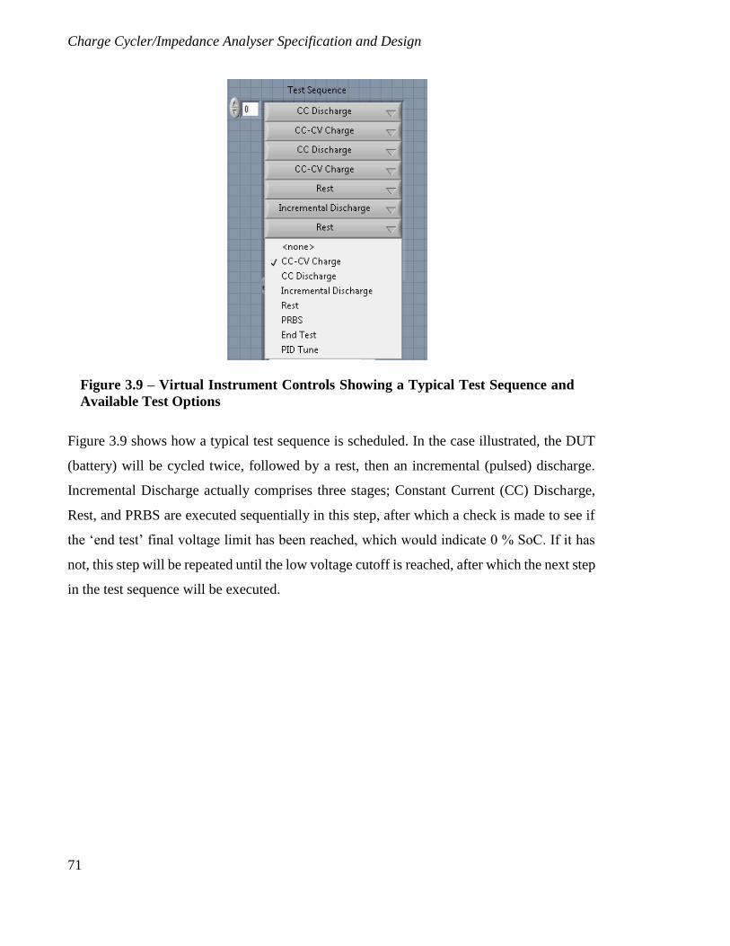
Charge Cycler/Impedance Analyser Specification and Design
71
Figure 3.9 shows how a typical test sequence is scheduled. In the case illustrated, the DUT
(battery) will be cycled twice, followed by a rest, then an incremental (pulsed) discharge.
Incremental Discharge actually comprises three stages; Constant Current (CC) Discharge,
Rest, and PRBS are executed sequentially in this step, after which a check is made to see if
the ‘end test’ final voltage limit has been reached, which would indicate 0 % SoC. If it has
not, this step will be repeated until the low voltage cutoff is reached, after which the next step
in the test sequence will be executed.
Figure 3.9 – Virtual Instrument Controls Showing a Typical Test Sequence and
Available Test Options
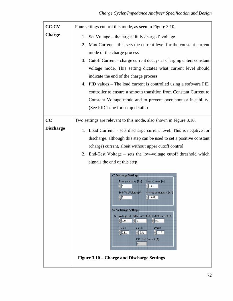
Charge Cycler/Impedance Analyser Specification and Design
72
CC-CV
Charge
Four settings control this mode, as seen in Figure 3.10.
1. Set Voltage – the target ‘fully charged’ voltage
2. Max Current – this sets the current level for the constant current
mode of the charge process
3. Cutoff Current – charge current decays as charging enters constant
voltage mode. This setting dictates what current level should
indicate the end of the charge process
4. PID values – The load current is controlled using a software PID
controller to ensure a smooth transition from Constant Current to
Constant Voltage mode and to prevent overshoot or instability.
(See PID Tune for setup details)
CC
Discharge
Two settings are relevant to this mode, also shown in Figure 3.10.
1. Load Current - sets discharge current level. This is negative for
discharge, although this step can be used to set a positive constant
(charge) current, albeit without upper cutoff control
2. End-Test Voltage – sets the low-voltage cutoff threshold which
signals the end of this step
Figure 3.10 – Charge and Discharge Settings
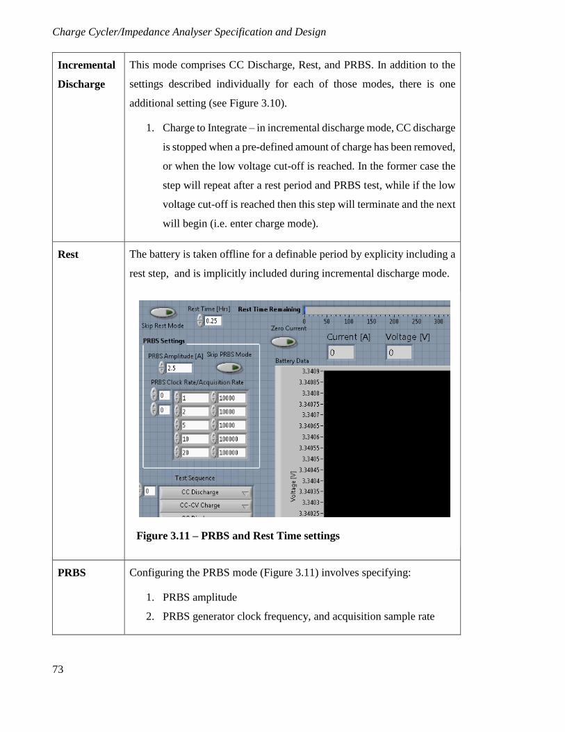
Charge Cycler/Impedance Analyser Specification and Design
73
Incremental
Discharge
This mode comprises CC Discharge, Rest, and PRBS. In addition to the
settings described individually for each of those modes, there is one
additional setting (see Figure 3.10).
1. Charge to Integrate – in incremental discharge mode, CC discharge
is stopped when a pre-defined amount of charge has been removed,
or when the low voltage cut-off is reached. In the former case the
step will repeat after a rest period and PRBS test, while if the low
voltage cut-off is reached then this step will terminate and the next
will begin (i.e. enter charge mode).
Rest The battery is taken offline for a definable period by explicity including a
rest step, and is implicitly included during incremental discharge mode.
PRBS Configuring the PRBS mode (Figure 3.11) involves specifying:
1. PRBS amplitude
2. PRBS generator clock frequency, and acquisition sample rate
Figure 3.11 – PRBS and Rest Time settings
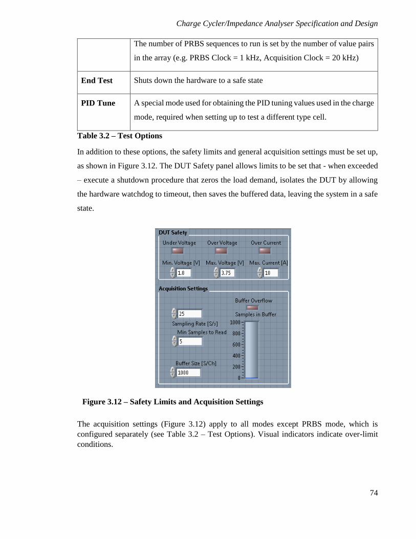
Charge Cycler/Impedance Analyser Specification and Design
74
The number of PRBS sequences to run is set by the number of value pairs
in the array (e.g. PRBS Clock = 1 kHz, Acquisition Clock = 20 kHz)
End Test Shuts down the hardware to a safe state
PID Tune A special mode used for obtaining the PID tuning values used in the charge
mode, required when setting up to test a different type cell.
Table 3.2 – Test Options
In addition to these options, the safety limits and general acquisition settings must be set up,
as shown in Figure 3.12. The DUT Safety panel allows limits to be set that - when exceeded
– execute a shutdown procedure that zeros the load demand, isolates the DUT by allowing
the hardware watchdog to timeout, then saves the buffered data, leaving the system in a safe
state.
The acquisition settings (Figure 3.12) apply to all modes except PRBS mode, which is
configured separately (see Table 3.2 – Test Options). Visual indicators indicate over-limit
conditions.
Figure 3.12 – Safety Limits and Acquisition Settings
Charge Cycler/Impedance Analyser Specification and Design
75
3.4.2 PRBS Post-Processing
Post processing has been streamlined in the new software, so that impedance results are
available immediately at the conclusion of the test. Synchronising the PRBS clock with the
data acquisition clock removed the need to use autocorrelation to identify the start and finish
points of the PRBS streams, since these points can be directly indexed in the set of acquired
samples.
The process for each PRBS clock frequency is to take the FFT of the voltage response and
divide point-by-point with the FFT of the current stimulus. This is repeated for each set of
time domain PRBS test results, and these impedance spectrums are then sliced to exclude all
frequencies above roughly 1/3rd of the obtained bandwidth (see Chapter 1; higher frequencies
produce impedance data which suffers with poor SNR).
Typically, the PRBS test is set up to repeat at a logarithmic spread of frequencies, e.g. [1, 2,
5, 10, 20, 50, 100, 200, 500, 1k, 2k, 5k, 10k, 20k], producing 14 impedance spectra, each
overlapping with its lower frequency neighbours. These band-limited results are then
interpolated, averaged and smoothed using a moving average to produce a single continuous
impedance spectrum.
Charge Cycler/Impedance Analyser Specification and Design
76
3.5 Hardware Performance Characteristics
The equipment has been empirically validated to meet the following conditions (see earlier
section for theoretical limits):
3.5.1 Charge Cycling and Pulsed Discharge
Figure 3.13 shows the test log from a charge cycling and pulsed discharge test on a 3 Ah
LFP26650E cell. The steps can clearly be identified; a constant-current charge mode is
followed by a constant voltage mode, followed by a complete discharge, then a full charge
which is followed by a rest period. Here a PRBS impedance test may be performed, followed
by a sequence of incremental (pulsed) discharge/rest/PRBS until the low-voltage cut-off is
reached. The last section is a charge to approximately 40% SOC, which is the standard SOC
level Li-ion cells should be stored at to reduce damage from internal stresses.
The charge curve resets to zero after each step change to minimise cumulative errors and
shows the change in absolute charge per step; the observed capacity of this cell when cycled
at 1 C is in fact 2.51 Ah. The pulsed discharger was set to remove charge in blocks of 0.6 Ah
(20% of nominal capacity), therefore the charge removed per pulse is 20 % of nominal
capacity, or 0.6 Ah
2.51 Ah = 23.9 % of actual capacity where present SoH is taken into account.
Original Specification Tested Specification
DUT Voltage Range 1.5 V – 6 V 0 V – 7.4 V
DUT Current Range ± 5 A +/- 8A
Acquisition Sample
Rate
10 kHz desirable, 5kHz
acceptable
100 kHz
NI USB-DAQ 6211 Synchronised simultaneous
V and I measurement ADCs
Inter-channel Delay =
minimum 4µs
Synchronised sample and
PRBS clock
Yes
Table 3.3 – Tested Specifications
Charge Cycler/Impedance Analyser Specification and Design
77
Also observable in Figure 3.13 is the smooth transition from constant current charging to
constant voltage charging. This is achieved by use of software PID control (described in
section 3.4) to monitor the charge voltage and control the charge current to prevent overshoot
and maintain a set voltage until the charge current is reduced sufficiently to indicate a full
charge.
Calibration of the bulk charge cycling function is checked using an external voltmeter and
ammeter, and can be corrected easily using scaling functions within the LabVIEW VI.
Figure 3.13 – Charge Cycling and Pulsed Discharge, 26650E Cell
Charge Cycler/Impedance Analyser Specification and Design
78
3.5.2 PRBS – Time Domain Signals
Figure 3.14 shows the stimulus and response curves for an 8 A peak, 1 Hz PRBS which is 63
bits long. This system test was performed on a 50 Ah Lithium Titanate (LTO) Super Lithium
Polymer Battery (SLPB) cell, and this figure, when compared with Figure 2.17, highlights
the improved SNR that has been achieved with this design when testing high capacity cells.
The high frequency validation test results shown in Figure 3.15 provide a visual measure of
the performance and demonstrate that the system is stable at these higher frequencies. The
maximum acquisition rate of the system is 100 kS/s, although as the PRBS clock rate was
increased beyond 35 kHz the time domain signal was observed to distort, and frequency
analysis showed a sharp increase in noise when plotting the phase of the impedance. The
frequency response is discussed in the next section.
Figure 3.14 – Demonstration of 8 A amplitude PRBS, 1Hz PRBS Clock
Charge Cycler/Impedance Analyser Specification and Design
79
a)
b)
Figure 3.15 – Distortion as PRBS Clock (35 kHz) Approaches the Nyquist Limit (50
kHz)
Charge Cycler/Impedance Analyser Specification and Design
80
3.5.3 PRBS – Frequency Response
The frequency response was evaluated by measuring the frequency response of a parallel RC
circuit and comparing the response with that of industry standard Solartron 1480 EIS test
equipment.
The results shown in Figure 3.16 show that the PRBS test has captured the characteristic
semicircle of a parallel RC circuit. The low frequency points (right hand side) show good
correlation with the EIS data (1.07 % error in real component, 0.17 % error in imaginary
component), but these errors increase with frequency. Points on the Nyquist plot are not
easily correlated to specific frequencies, therefore further analysis of errors is done on the
amplitude and phase plots of Figure 3.17.
Figure 3.16 – Nyquist Plot of Parallel RC Circuit Validation Test
0 0.2 0.4 0.6 0.8 1
-0.5
-0.4
-0.3
-0.2
-0.1
0
0.1
0.2
0.3
Parallel RC Impedance
Z(Real),
Z(I
mag
),
EIS data
PRBS data (smoothed)
PRBS data
Charge Cycler/Impedance Analyser Specification and Design
81
a)
b)
Figure 3.17 – Validation Test: Parallel RC Impedance plots, R = 1 Ω, C = 10 mF
10-2
10-1
100
101
102
103
104
0
0.2
0.4
0.6
0.8
1
1.2
1.4
Parallel RC Impedance
Frequency, Hz
Am
plitu
de,
EIS data
PRBS data (smoothed)
PRBS data
10-2
10-1
100
101
102
103
104
-90
-80
-70
-60
-50
-40
-30
-20
-10
0
10
Frequency, Hz
Ph
ase,
Parallel RC Impedance
EIS data
PRBS data (smoothed)
PRBS data
Charge Cycler/Impedance Analyser Specification and Design
82
Figure 3.17 shows that for frequencies below 100 Hz, there is good correlation between the
standard data and the validation test data. The corner frequency of the circuit is at
approximately 15 Hz, and we can observe that this corresponds with a single peak in the
amplitude deviation shown in Figure 3.18. During testing, the 200 Hz and 500 Hz PRBS tests
were unfortunately not set; it is possible that this error will be reduced if the results of these
test frequencies were included, as the data from these sequences (covering 3.1 Hz to 88 Hz,
and 7.9 Hz to 222 Hz) would provide the best SNR over the corner frequency. Further work
should begin with this step.
Below 100 Hz the phase error is consistently less than 4 ˚. Above this frequency the error
increases dramatically, but also appears to be increasing fairly linearly, at a rate of 24 ˚ per
decade between 100 Hz and 1 kHz. This points to a systematic error, and is likely to be due
to the inter-channel measurement delay. There was no time to investigate this further, but a
quick calculation (delay=phase/frequency) shows that a phase error of 24° at 1 kHz
Figure 3.18 – Absolute Error between EIS and PRBS RC Impedance Data
10-1
100
101
102
103
0
0.02
0.04
0.06
Absolute Error Between EIS RC Impedance Data and PRBS Data
Frequency, Hz
Am
pli
tud
e E
rror,
10-1
100
101
102
103
0
8
16
24
32
40
48
56
60
Ph
ase
Error,
Phase Error,
Amplitude Error,
Charge Cycler/Impedance Analyser Specification and Design
83
corresponds to a time delay of 66 μs. The acquisition system used has a minimum inter-
channel delay of 4 µs, and a preferred 10 µs settling time between reading each channel. With
two differential inputs (four channels) to read, this delay time is most likely the cause of the
observed phase error; more tests will be required to prove this.
3.6 Example Results
Figure 3.19 and Figure 3.20 are the results of a one-off impedance test of a 50 Ah, 2.3 V nano
Lithium-Titanate cell. The characteristic semicircle due to the parallel RC nature of the cell
model is clearly identifiable in the Nyquist plot, and represents the RC element of the charge
transfer resistance model. The effect of 7.5 % SoC change is prominently visible at
frequencies below 10 Hz.
Figure 3.19 – Impedance Data from a Large Capacity Cell
Charge Cycler/Impedance Analyser Specification and Design
84
3.7 Conclusion
Early findings have been discussed in section 2.7, Preliminary Findings and Suggested
Changes. The new impedance test equipment meets the design specification, and performs
well at the low frequencies which are of interest in the analysis of battery dynamics. At higher
frequencies, while the impedance amplitude data is reliable, the phase data presented here is
not. This is believed to be due to the inter-channel measurement delay caused by multiplexing
signals to a single ADC. The delay time was significantly reduced in the second design,
though it is recommended that simultaneous acquisition is used for further work.
Synchronising the measurement sampling and PRBS generation has enabled a more a robust
procedure for capturing good quality results, as has the ability to test higher capacity cells at
larger stimulus current levels.
Figure 3.20 – Nyquist Plot of Impedance, 50 Ah SLPB cell

85
Chapter 4: Conclusions and Suggestions for Further Work
4.1 Conclusions
The first chapter was a brief overview of popular EV battery chemistries, with a functional
description of Battery Management Systems and battery state estimation techniques.
Electrochemical Impedance Spectroscopy was introduced as a system identification tool and
we showed how Pseudo-Random Binary Sequences can be used as a system stimulus
approximating white noise, giving the benefits of wide-bandwidth system identification with
the convenience of a short test duration.
Chapter 2 described the development of equipment to cycle charge and measure the
impedance of a range of Li-ion cells. The results of tests on two types of cell, LFP 26650E
3 Ah cells and LTO polymer 100 Ah pouch cells, are presented along with an analysis of the
weaknesses found in the early system which prompted a redesign and new methods. This can
be found in section 2.7, but the main findings from the first system are summarised here:
1) Charge Cycling
a) When cycling higher voltage battery packs high frequency oscillations could not be
prevented. For this reason we were not able to map the maximum power
characteristics of the cell, although low voltage (3.7 V) single cells were successfully
cycled at rates of 20 A (C/5) using a single output channel.
b) The above stability problems meant that cells sometimes had to be charged using a
bench power supply directly, and some charging data was lost as a result. The ability
to compare charging capacity against discharging capacity would be useful to provide
an analysis of cell dynamic characteristics and forming bi-directional models.
c) An oversight in the initial setup was not to continuously log the cell terminal voltage
as it settled during the voltage relaxation step of a pulsed discharge. Without this data
we cannot attempt to compensate for any insufficiency in settling time by means of
extrapolation.
2) PRBS Impedance Testing
a) The PRBS generation clock and data acquisition clock must be synchronised; the
inter-channel delay of the acquisition system was discovered to be up to 12 % of the
Conclusions and Suggestions for Further Work
86
PRBS clock period and 60 % of the acquisition period. This margin of error is
unacceptable for a PRBS analysis, where exact-length sequences are required for a
clean FFT.
b) Software timing is not a reliable method for generating a precise PRBS stream and
should be avoided.
c) Choosing the amplitude of a PRBS stimulus current requires making a trade-off
between obtaining a voltage response with good signal-to-noise ratio while
maintaining the cell in a steady state. Having bipolar stimulus capabilities allows the
stimulus current level to be increased while maintaining a steady state in the cell SoC
compared to a unipolar PRBS test.
d) Sensitive measurement instruments are not commonly available in very high cell-
count battery packs, where 5 mV resolution is considered to be good [52]. This must
be taken into consideration when designing an embedded impedance tester for very
low impedance cells such as high capacity LTO cells, for example.
These shortcomings are addressed in the second design iteration presented in Chapter 3. The
remaining problem with the system in Chapter 3 is believed to be again caused by the inter-
channel measurement delay which causes the phase error to become significant at higher
frequencies. This delay time (caused by multiplexing analogue inputs to a single ADC) was
reduced from 160 µs in the first design to perhaps 66 µs in the second, and is suspected to
account for the frequency dependent phase error seen in the second system (Figure 3.18 –
Absolute Error between EIS and PRBS RC Impedance Data).
4.2 Suggestions for Further Work
Further work should begin with an investigation of the effect that the inter-channel
measurement delay has on the existing system. Provided that the results are reproducible –
i.e. that the delay is constant – then a phase compensation scheme should be easy to
implement. If the delay is not constant or predictable, then the options are to design a sample-
and-hold acquisition system or else to obtain an acquisition system that contains at least four
individual ADCs and hence requires no input multiplexing.
The second suggestion for further work pertains to cell testing methods. We have seen that
for an impedance measurement to be useful for system identification then the SoC of the cell
Conclusions and Suggestions for Further Work
87
must not change significantly while making the measurement. If we quantify this and say
that the SoC must not change by more than say 1 % during a test, then using the PRBS test
time (say 100 seconds) we can define a discharge rate at which an injected PRBS ripple
would give meaningful impedance results. For example, using the figures above we could
say that a constant discharge at a rate of 𝐶 × 0.01 ×3600
100= 0.36𝐶 could be combined with a
bipolar (i.e. does not contribute to a mean change in charge) PRBS ripple to yield
approximately one hundred wide-band impedance readings over a full discharge. Clearly
these numbers would have to be refined empirically to account for the fact that the cell does
not discharge linearly, to keep the maximum SoC change during a PRBS within the set
tolerance. The advantages of such an approach include the ability to observe key changes in
impedance during a charge cycle at a relatively high resolution between states; furthermore
with charging impedances distinct from the impedances obtained during discharging then a
truly bi-directional model can be developed. The existing hardware is capable of performing
this experiment with only a slight software modification. The idea came from a paper [60] in
which the authors recorded the discharge characteristic of a cell discharged with a continuous
GSM power pulse, in order to assess the impact of the application on cell capacity.
One reason that PRBS is used as a stimulus signal is that it produces a flat wide-band power
spectrum. This is good for identifying unknown systems, but may be a disadvantage on a
known system. For example, if the largest changes in impedance occur in limited bands of
the spectrum – e.g. from 1 mHz to 5 Hz, and from 2 kHz to 8 kHz – then it may be
advantageous to switch to Binary Multi-frequency Signal stimulation. These signals
concentrate the power spectrum to specific frequency bands, giving better signal-to-noise
ratio in the areas of interest [65]. It would of course be easy to implement a Binary Multi-
frequency test with the present hardware.
We have detailed the design process, the shortcomings of the initial design and the steps
taken to overcome them. Within the third chapter are adequate details for the reader to
reproduce the system described here, and three ideas for further work have been given.
88
References
[1] J. Larminie and J. Lowry, Electric vehicle technology explained. J. Wiley, 2003.
[2] S. Vazquez, S. M. Lukic, E. Galvan, L. G. Franquelo, and J. M. Carrasco, “Energy
Storage Systems for Transport and Grid Applications,” Industrial Electronics, IEEE
Transactions on, vol. 57, no. 12, pp. 3881–3895, 2010.
[3] J. McDowall, “Integrating energy storage with wind power in weak electricity grids,”
Journal of Power Sources, vol. 162, no. 2, pp. 959–964, 2006.
[4] S. Bharadwaj, “Clean Energy Storage for Grid Load Leveling -The Metlakatla Battery
Energy Storage System - Twelve Years Of Success,” in Irena Conference, Port Vila,
2012.
[5] M. Farber_De_Anda, J. D. Boyes, and W. Torres, “Lessons Learned from the Puerto
Rico Battery Energy Storage System,” Sandia National Laboratories, 1999.
[6] “DIRECTIVE 2002/95/EC OF THE EUROPEAN PARLIAMENT AND OF THE
COUNCIL of 27 January 2003.” 2003.
[7] “Battery Recycling.” Battery Council International, 2009.
[8] N. Garimella and N.-K. C. Nair, “Assessment of battery energy storage systems for
small-scale renewable energy integration,” in TENCON 2009 - 2009 IEEE Region 10
Conference, 2009, pp. 1–6.
[9] O. Edberg and C. Naish, “Energy Storage and Management Study,” AEA Group for
Scottish Government, 2010.
[10] C. Naish, I. McCubbin, O. Edberg, and M. Harfoot, “Outlook of Energy Storage
Technologies,” European Parliament’s committee on Industry, Research and Energy
(ITRE), January 2004, 2008.
[11] B. Dunn, H. Kamath, and J.-M. Tarascon, “Electrical Energy Storage for the Grid: A
Battery of Choices,” Science, vol. 334, no. 6058, pp. 928–935, 2011.
[12] M. Duduta, B. Ho, V. C. Wood, P. Limthongkul, V. E. Brunini, W. C. Carter, and Y.-
M. Chiang, “Semi-Solid Lithium Rechargeable Flow Battery,” Advanced Energy
Materials, vol. 1, no. 4, pp. 511–516, 2011.
[13] A. Kraytsberg and Y. Ein-Eli, “Review on Li-air batteries: Opportunities, limitations
and perspective,” Journal of Power Sources, vol. 196, no. 3, pp. 886–893, 2011.
[14] B. Scrosati and J. Garche, “Lithium batteries: Status, prospects and future,” Journal of
Power Sources, vol. 195, no. 9, pp. 2419–2430, 2010.
[15] K. C. Divya and J. Ostergaard, “Battery energy storage technology for power systems
- An overview,” Electric Power Systems Research, vol. 79, no. 4, pp. 511–520, 2009.
[16] J. W. Fergus, “Recent developments in cathode materials for lithium ion batteries,”
Journal of Power Sources, vol. 195, no. 4, pp. 939–954, 2010.
[17] M. Armand and J.-M. J.-M. Tarascon, “Building better batteries,” Nature, vol. 451, no.
7179, pp. 652–657, 2008.
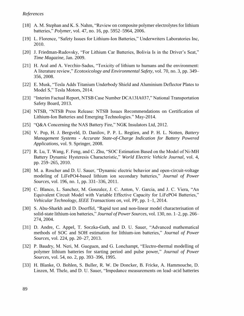
References
89
[18] A. M. Stephan and K. S. Nahm, “Review on composite polymer electrolytes for lithium
batteries,” Polymer, vol. 47, no. 16, pp. 5952–5964, 2006.
[19] L. Florence, “Safety Issues for Lithium-Ion Batteries,” Underwriters Laboratories Inc,
2010.
[20] J. Friedman-Rudovsky, “For Lithium Car Batteries, Bolivia Is in the Driver’s Seat,”
Time Magazine, Jan. 2009.
[21] H. Aral and A. Vecchio-Sadus, “Toxicity of lithium to humans and the environment:
A literature review,” Ecotoxicology and Environmental Safety, vol. 70, no. 3, pp. 349–
356, 2008.
[22] E. Musk, “Tesla Adds Titanium Underbody Shield and Aluminium Deflector Plates to
Model S,” Tesla Motors, 2014.
[23] “Interim Factual Report, NTSB Case Number DCA13IA037,” National Transportation
Safety Board, 2013.
[24] NTSB, “NTSB Press Release: NTSB Issues Recommendations on Certification of
Lithium-Ion Batteries and Emerging Technologies.” May-2014.
[25] “Q&A Concerning the NAS Battery Fire,” NGK Insulators Ltd, 2012.
[26] V. Pop, H. J. Bergveld, D. Danilov, P. P. L. Regtien, and P. H. L. Notten, Battery
Management Systems - Accurate State-of-Charge Indication for Battery Powered
Applications, vol. 9. Springer, 2008.
[27] R. Lu, T. Wang, F. Feng, and C. Zhu, “SOC Estimation Based on the Model of Ni-MH
Battery Dynamic Hysteresis Characteristic,” World Electric Vehicle Journal, vol. 4,
pp. 259–265, 2010.
[28] M. a. Roscher and D. U. Sauer, “Dynamic electric behavior and open-circuit-voltage
modeling of LiFePO4-based lithium ion secondary batteries,” Journal of Power
Sources, vol. 196, no. 1, pp. 331–336, 2011.
[29] C. Blanco, L. Sanchez, M. Gonzalez, J. C. Anton, V. Garcia, and J. C. Viera, “An
Equivalent Circuit Model with Variable Effective Capacity for LiFePO4 Batteries,”
Vehicular Technology, IEEE Transactions on, vol. PP, pp. 1–1, 2014.
[30] S. Abu-Sharkh and D. Doerffel, “Rapid test and non-linear model characterisation of
solid-state lithium-ion batteries,” Journal of Power Sources, vol. 130, no. 1–2, pp. 266–
274, 2004.
[31] D. Andre, C. Appel, T. Soczka-Guth, and D. U. Sauer, “Advanced mathematical
methods of SOC and SOH estimation for lithium-ion batteries,” Journal of Power
Sources, vol. 224, pp. 20–27, 2013.
[32] P. Baudry, M. Neri, M. Gueguen, and G. Lonchampt, “Electro-thermal modelling of
polymer lithium batteries for starting period and pulse power,” Journal of Power
Sources, vol. 54, no. 2, pp. 393–396, 1995.
[33] H. Blanke, O. Bohlen, S. Buller, R. W. De Doncker, B. Fricke, A. Hammouche, D.
Linzen, M. Thele, and D. U. Sauer, “Impedance measurements on lead–acid batteries
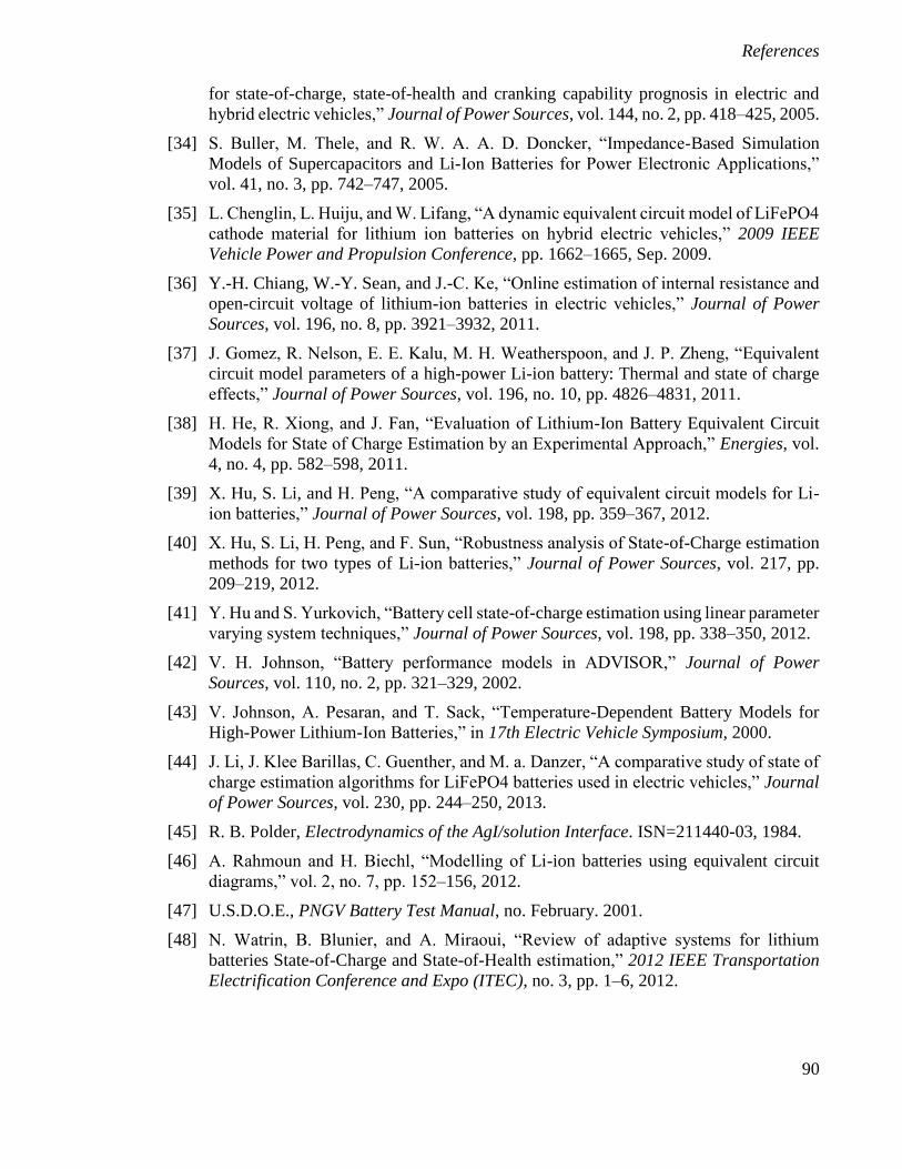
References
90
for state-of-charge, state-of-health and cranking capability prognosis in electric and
hybrid electric vehicles,” Journal of Power Sources, vol. 144, no. 2, pp. 418–425, 2005.
[34] S. Buller, M. Thele, and R. W. A. A. D. Doncker, “Impedance-Based Simulation
Models of Supercapacitors and Li-Ion Batteries for Power Electronic Applications,”
vol. 41, no. 3, pp. 742–747, 2005.
[35] L. Chenglin, L. Huiju, and W. Lifang, “A dynamic equivalent circuit model of LiFePO4
cathode material for lithium ion batteries on hybrid electric vehicles,” 2009 IEEE
Vehicle Power and Propulsion Conference, pp. 1662–1665, Sep. 2009.
[36] Y.-H. Chiang, W.-Y. Sean, and J.-C. Ke, “Online estimation of internal resistance and
open-circuit voltage of lithium-ion batteries in electric vehicles,” Journal of Power
Sources, vol. 196, no. 8, pp. 3921–3932, 2011.
[37] J. Gomez, R. Nelson, E. E. Kalu, M. H. Weatherspoon, and J. P. Zheng, “Equivalent
circuit model parameters of a high-power Li-ion battery: Thermal and state of charge
effects,” Journal of Power Sources, vol. 196, no. 10, pp. 4826–4831, 2011.
[38] H. He, R. Xiong, and J. Fan, “Evaluation of Lithium-Ion Battery Equivalent Circuit
Models for State of Charge Estimation by an Experimental Approach,” Energies, vol.
4, no. 4, pp. 582–598, 2011.
[39] X. Hu, S. Li, and H. Peng, “A comparative study of equivalent circuit models for Li-
ion batteries,” Journal of Power Sources, vol. 198, pp. 359–367, 2012.
[40] X. Hu, S. Li, H. Peng, and F. Sun, “Robustness analysis of State-of-Charge estimation
methods for two types of Li-ion batteries,” Journal of Power Sources, vol. 217, pp.
209–219, 2012.
[41] Y. Hu and S. Yurkovich, “Battery cell state-of-charge estimation using linear parameter
varying system techniques,” Journal of Power Sources, vol. 198, pp. 338–350, 2012.
[42] V. H. Johnson, “Battery performance models in ADVISOR,” Journal of Power
Sources, vol. 110, no. 2, pp. 321–329, 2002.
[43] V. Johnson, A. Pesaran, and T. Sack, “Temperature-Dependent Battery Models for
High-Power Lithium-Ion Batteries,” in 17th Electric Vehicle Symposium, 2000.
[44] J. Li, J. Klee Barillas, C. Guenther, and M. a. Danzer, “A comparative study of state of
charge estimation algorithms for LiFePO4 batteries used in electric vehicles,” Journal
of Power Sources, vol. 230, pp. 244–250, 2013.
[45] R. B. Polder, Electrodynamics of the AgI/solution Interface. ISN=211440-03, 1984.
[46] A. Rahmoun and H. Biechl, “Modelling of Li-ion batteries using equivalent circuit
diagrams,” vol. 2, no. 7, pp. 152–156, 2012.
[47] U.S.D.O.E., PNGV Battery Test Manual, no. February. 2001.
[48] N. Watrin, B. Blunier, and A. Miraoui, “Review of adaptive systems for lithium
batteries State-of-Charge and State-of-Health estimation,” 2012 IEEE Transportation
Electrification Conference and Expo (ITEC), no. 3, pp. 1–6, 2012.
References
91
[49] J. D. Kozlowski, “Electrochemical cell prognostics using online impedance
measurements and model-based data fusion techniques,” in Aerospace Conference,
2003. Proceedings. 2003 IEEE, 2003, vol. 7, pp. 3257–3270.
[50] A. J. Salkind, C. Fennie, P. Singh, T. Atwater, and D. E. Reisner, “Determination of
state-of-charge and state-of-health of batteries by fuzzy logic methodology,” Journal
of Power Sources, vol. 80, no. 1–2, pp. 293–300, 1999.
[51] P. Singh and C. F. Jr, “Fuzzy logic-enhanced electrochemical impedance spectroscopy
(FLEEIS) to determine battery state-of-charge,” Battery Conference on …, 2000.
[52] L. Lu, X. Han, J. Li, J. Hua, and M. Ouyang, “A review on the key issues for lithium-
ion battery management in electric vehicles,” Journal of Power Sources, vol. 226, pp.
272–288, 2013.
[53] O. Gerard, J.-N. Patillon, and F. d Alche-Buc, “Neural network adaptive modeling of
battery discharge behavior,” in Artificial Neural Networks - ICANN’97, vol. 1327, W.
Gerstner, A. Germond, M. Hasler, and J.-D. Nicoud, Eds. Springer Berlin Heidelberg,
1997, pp. 1095–1100.
[54] B. S. Bhangu, P. Bentley, D. A. Stone, and C. M. Bingham, “Observer techniques for
estimating the state-of-charge and state-of-health of VRLABs for hybrid electric
vehicles,” in Vehicle Power and Propulsion, 2005 IEEE Conference, 2005, p. 10 pp.
[55] B. S. Bhangu, P. Bentley, D. A. Stone, and C. M. Bingham, “State-of-charge and state-
of-health prediction of lead-acid batteries for hybrid electric vehicles using non-linear
observers,” in Power Electronics and Applications, 2005 European Conference on,
2005, p. 10 pp. –P.10.
[56] B. S. Bhangu, P. Bentley, D. A. Stone, and C. M. Bingham, “Nonlinear observers for
predicting state-of-charge and state-of-health of lead-acid batteries for hybrid-electric
vehicles,” Vehicular Technology, IEEE Transactions on, vol. 54, no. 3, pp. 783–794,
2005.
[57] C. Gould, J. Wang, D. Stone, and M. Foster, “EV/HEV Li-ion battery modelling and
State-of-Function determination,” International Symposium on Power Electronics
Power Electronics, Electrical Drives, Automation and Motion, pp. 353–358, 2012.
[58] C. R. Gould, C. M. Bingham, D. A. Stone, and P. Bentley, “New Battery Model and
State-of-Health Determination Through Subspace Parameter Estimation and State-
Observer Techniques,” Vehicular Technology, IEEE Transactions on, vol. 58, no. 8,
pp. 3905–3916, 2009.
[59] J. L. Lee, A. Chemistruck, and G. L. Plett, “One-dimensional physics-based reduced-
order model of lithium-ion dynamics,” Journal of Power Sources, vol. 220, pp. 430–
448, 2012.
[60] A. Jossen, “Fundamentals of battery dynamics,” Journal of Power Sources, vol. 154,
no. 2, pp. 530–538, 2006.
[61] B. Sanchez, G. Vandersteen, R. Bragos, and J. Schoukens, “Basics of broadband
impedance spectroscopy measurements using periodic excitations,” Measurement
Science and Technology, vol. 23, no. 10, p. 105501, 2012.
References
92
[62] E. Barsoukov and J. R. Macdonald, Eds., Impedance Spectroscopy - Theory,
Experiment and Applications. Wiley, 2005.
[63] W. D. T. Davies, “Using the binary maximum length sequence for the identification of
system dynamics,” Electrical Engineers, Proceedings of the Institution of, vol. 114, no.
10, pp. 1582–1584, 1967.
[64] J. Schoukens, R. M. Pintelon, and Y. J. Rolain, “Broadband versus stepped sine FRF
measurements,” IEEE Transactions on Instrumentation and Measurement, vol. 49, no.
2, pp. 275–278, 2000.
[65] K. Godfrey, “Introduction to binary signals used in system identification,” in Control
1991. Control’91., International Conference on, 1991, pp. 161–166.
[66] A. J. Fairweather, M. P. Foster, and D. A. Stone, “Battery parameter identification with
Pseudo Random Binary Sequence excitation (PRBS),” Journal of Power Sources, vol.
196, no. 22, pp. 9398–9406, 2011.
[67] A. J. Fairweather, M. P. Foster, and D. A. Stone, “VRLA battery parameter
identification using pseudo random binary sequences (PRBS),” in Power Electronics,
Machines and Drives (PEMD 2010), 5th IET International Conference on, 2010, pp.
1–6.
93
Appendix 1.
Figure A. 1 – 26650E Cell OCV vs. SoC for each Cell Configuration
01020304050607080901002.6
2.7
2.8
2.9
3
3.1
3.2
3.3
3.4
3.5
3.6
Normalised SoC (%)
OC
V (
V)
26650 3Ah LiFePO4 Cell #1: OCV vs SoC
10 degrees C
20 degrees C
30 degrees C
01020304050607080901002.6
2.7
2.8
2.9
3
3.1
3.2
3.3
3.4
3.5
3.6
Normalised SoC (%)
OC
V (
V)
26650 3Ah LiFePO4 Cell #2: OCV vs SoC
10 degrees C
20 degrees C
30 degrees C
40 degrees C
50 degrees C
01020304050607080901002.6
2.7
2.8
2.9
3
3.1
3.2
3.3
3.4
3.5
3.6
Normalised SoC (%)
OC
V (
V)
26650 3Ah LiFePO4 Cell #3: OCV vs SoC
10 degrees C
20 degrees C
30 degrees C
40 degrees C
50 degrees C
01020304050607080901002.6
2.7
2.8
2.9
3
3.1
3.2
3.3
3.4
3.5
3.6
Normalised SoC (%)
OC
V (
V)
26650 3Ah LiFePO4 Cell #4: OCV vs SoC
10 degrees C
20 degrees C
30 degrees C
40 degrees C
50 degrees C
01020304050607080901002.6
2.7
2.8
2.9
3
3.1
3.2
3.3
3.4
3.5
3.6
Normalised SoC (%)
OC
V (
V)
26650 3Ah LiFePO4 Cells 2 & 3 Parallel: OCV vs SoC
10 degrees C
20 degrees C
30 degrees C
40 degrees C
50 degrees C
01020304050607080901002.6
2.7
2.8
2.9
3
3.1
3.2
3.3
3.4
3.5
3.6
Normalised SoC (%)
OC
V (
V)
26650 3Ah LiFePO4 Cells 2,3 & 4 Parallel: OCV vs SoC
10 degrees C
20 degrees C
30 degrees C
40 degrees C
50 degrees C
Appendix 1
94
Figure A. 2 – 26650E Cells: OCV vs. SoC at Fixed Temperatures, Comparing Cells
01020304050607080901002.6
2.7
2.8
2.9
3
3.1
3.2
3.3
3.4
3.5
3.6
Normalised SoC (%)
OC
V (
V)
26650 3Ah LiFePO4 Cells at 10 degrees C: OCV vs SoC
Cell #1
Cell #2
Cell #3
Cell #4
Cell #5
Cell #23
Cell #234
01020304050607080901002.6
2.7
2.8
2.9
3
3.1
3.2
3.3
3.4
3.5
3.6
Normalised SoC (%)
OC
V (
V)
26650 3Ah LiFePO4 Cells at 20 degrees C: OCV vs SoC
Cell #1
Cell #2
Cell #3
Cell #4
Cell #5
Cell #23
Cell #234
01020304050607080901002.6
2.7
2.8
2.9
3
3.1
3.2
3.3
3.4
3.5
3.6
Normalised SoC (%)
OC
V (
V)
26650 3Ah LiFePO4 Cells at 30 degrees C: OCV vs SoC
Cell #1
Cell #2
Cell #3
Cell #4
Cell #5
Cell #23
Cell #234
01020304050607080901002.6
2.7
2.8
2.9
3
3.1
3.2
3.3
3.4
3.5
3.6
Normalised SoC (%)
OC
V (
V)
26650 3Ah LiFePO4 Cells at 40 degrees C: OCV vs SoC
Cell #2
Cell #3
Cell #4
Cell #5
Cell #23
Cell #234
01020304050607080901002.6
2.7
2.8
2.9
3
3.1
3.2
3.3
3.4
3.5
3.6
Normalised SoC (%)
OC
V (
V)
26650 3Ah LiFePO4 Cells at 50 degrees C: OCV vs SoC
Cell #2
Cell #3
Cell #4
Cell #5
Cell #23
Cell #234
Appendix 1
95
Figure A. 3 – 26650E Cells: Average Impedance at 0-0.5 Hz vs. SoC for each Cell
Configuration
01020304050607080901000
0.02
0.04
0.06
0.08
0.1
0.12
0.14
0.16
0.18
0.2
Normalised SoC (%)
Impedance (
Ohm
s)
26650 3Ah LiFePO4 Cell #1: Impedance vs SoC
10 degrees C
20 degrees C
30 degrees C
01020304050607080901000
0.02
0.04
0.06
0.08
0.1
0.12
0.14
0.16
0.18
0.2
Normalised SoC (%)
Impedance (
Ohm
s)
26650 3Ah LiFePO4 Cell #2: Impedance vs SoC
10 degrees C
20 degrees C
30 degrees C
40 degrees C
50 degrees C
01020304050607080901000
0.02
0.04
0.06
0.08
0.1
0.12
0.14
0.16
0.18
0.2
Normalised SoC (%)
Impedance (
Ohm
s)
26650 3Ah LiFePO4 Cell #3: Impedance vs SoC
10 degrees C
20 degrees C
30 degrees C
40 degrees C
50 degrees C
01020304050607080901000
0.02
0.04
0.06
0.08
0.1
0.12
0.14
0.16
0.18
0.2
Normalised SoC (%)
Impedance (
Ohm
s)
26650 3Ah LiFePO4 Cell #4: Impedance vs SoC
10 degrees C
20 degrees C
30 degrees C
40 degrees C
50 degrees C
01020304050607080901000
0.02
0.04
0.06
0.08
0.1
0.12
0.14
0.16
0.18
0.2
Normalised SoC (%)
Impedance (
Ohm
s)
26650 3Ah LiFePO4 Cells 2 & 3: Impedance vs SoC
10 degrees C
20 degrees C
30 degrees C
40 degrees C
50 degrees C
01020304050607080901000
0.02
0.04
0.06
0.08
0.1
0.12
0.14
0.16
0.18
0.2
Normalised SoC (%)
Impedance (
Ohm
s)
26650 3Ah LiFePO4 Cells 2,3 & 4: Impedance vs SoC
10 degrees C
20 degrees C
30 degrees C
40 degrees C
50 degrees C
Appendix 1
96
Figure A. 4 - 26650E Cell Comparison at Fixed Temperature: Average Impedance at
0-0.5 Hz vs. SoC
01020304050607080901000
0.02
0.04
0.06
0.08
0.1
0.12
0.14
0.16
0.18
0.2
Normalised SoC (%)
Impedance (
Ohm
s)
26650 3Ah LiFePO4 Cells at 10 degrees C: Impedance vs SoC
Cell #1
Cell #2
Cell #3
Cell #4
Cell #5
Cell #23
Cell #234
01020304050607080901000
0.02
0.04
0.06
0.08
0.1
0.12
0.14
0.16
0.18
0.2
Normalised SoC (%)
Impedance (
Ohm
s)
26650 3Ah LiFePO4 Cells at 20 degrees C: Impedance vs SoC
Cell #1
Cell #2
Cell #3
Cell #4
Cell #5
Cell #23
Cell #234
01020304050607080901000
0.02
0.04
0.06
0.08
0.1
0.12
0.14
0.16
0.18
0.2
Normalised SoC (%)
Impedance (
Ohm
s)
26650 3Ah LiFePO4 Cells at 30 degrees C: Impedance vs SoC
Cell #1
Cell #2
Cell #3
Cell #4
Cell #5
Cell #23
Cell #234
01020304050607080901000
0.02
0.04
0.06
0.08
0.1
0.12
0.14
0.16
0.18
0.2
Normalised SoC (%)
Impedance (
Ohm
s)
26650 3Ah LiFePO4 Cells at 40 degrees C: Impedance vs SoC
Cell #2
Cell #3
Cell #4
Cell #5
Cell #23
Cell #234
01020304050607080901000
0.02
0.04
0.06
0.08
0.1
0.12
0.14
0.16
0.18
0.2
Normalised SoC (%)
Impedance (
Ohm
s)
26650 3Ah LiFePO4 Cells at 50 degrees C: Impedance vs SoC
Cell #2
Cell #3
Cell #4
Cell #5
Cell #23
Cell #234