Bass Connections in Energy - Spring 2016 Electric Vehicle ... · After thorough refinement of the body design via aerodynamics simulations, ergonomics studies, and aesthetic aspirations,

Bass Connections in Energy - Spring 2016

Electric Vehicle Team

Technical Report

Kathryn Abendroth, Max Feidelson, Charlie Kritzmacher

Abraham Ng’hwani, Anny Ning, Henry Miller, Evan Savell

With special thanks to Dr. Josiah Knight, Dr. Emily Klein, Steve Earp and Greg Bumpass,

Patrick McGuire, Michael Blagg, Bass Connections, and the Duke Electric Vehicles team

Table of Contents:

I. Executive Summary

II. Rear Suspension

A. Prototype Design

B. Testing

1. Experimental Setup

2. Test Data

C. MATLAB calculations (force loads under various driving conditions)

1. Resting weight & cornering

2. Braking

D. FEA results (maximum stress/ displacement in suspension)

1. Resting weight

2. Braking

3. Cornering

III. Carbon Fiber and Honeycomb Testing

A. Bending test procedure

1. Sample descriptions

B. Testing data (force vs displacement)

1. Average Young’s Modulus

2. Average yield strength

C. FEA results (maximum stress/ displacement in body for uniform material)

1. Resting weight

2. Braking

3. Cornering

D. MATLAB calculations (actual maximum stress in composite material)

1. Resting weight

2. Braking

3. Cornering

IV. Conclusions and Future Modifications

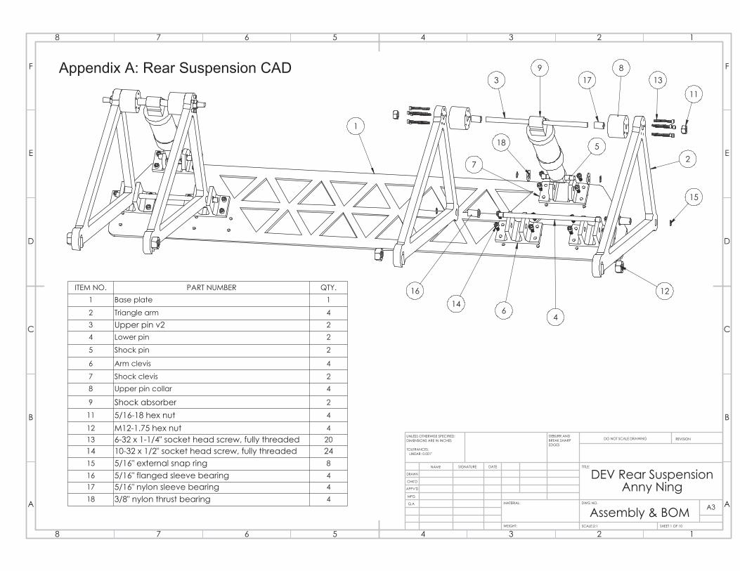
Appendix A: Rear Suspension CAD

1. Exploded assembly drawing with bill of materials

2. Machining drawings

Appendix B: MATLAB Script for Force Loads

Appendix C: MATLAB Script for Suspension Tests

Appendix D: Derivation of Equations

Appendix E: Sample Testing Data

2

I. Executive Summary

The Bass Connections Electric Vehicle Team designated three main components for the

development of sustainable transportation. The most technical of these goals was to design

and build a prototype of an urban concept electric vehicle for Duke Electric Vehicles (DEV).

The focus of this report is to address the various challenges and goals of the urban concept

vehicle.

The urban concept provides an opportunity for DEV to showcase some of its most

progressive and inventive engineering feats. The urban concept will be considered a flagship

vehicle for its most novel pursuits. In addition to building upon DEV’s previous work with

carbon fiber composite materials and monocoque designs, the urban concept is undergoing

more extensive finite element analysis (FEA) through SolidWorks. Said FEA was utilized to

test the suspension in response to various road and driving conditions. It was also used to

determine the strength properties of the body of the urban concept. Last, but not least,

experimentation was conducted to document the mechanical behavior of the suspension.

After thorough refinement of the body design via aerodynamics simulations, ergonomics

studies, and aesthetic aspirations, the urban concept body was finalized and made into molds

for production. As this project continues in the 2016-2017 academic year, the students

engaged in it will build upon the work our team has done here. This team is proud to have

completed many of the most challenging aspects of the urban concept and to have set up the

resources for finishing it.

3

II. Rear Suspension

A. Prototype Design

The design for the rear suspension was inspired by a trailing link suspension, often found

supporting the rear wheel of mountain bikes (see fig. 1 below). This type of suspension is

ideal for mounting bike wheels, such as the ones being used for the Urban Concept v.1,

since it supports the wheel axle on both sides and thus reduces the cantilever effect on the

axle as it encounters impact forces.

Figure 1: Trailing link suspension on part of a mountain bike frame. The suspension used

in the Urban Concept v.1 was adapted from this design, placing the wheel in front of the

shock and separating the prismatic truss into two triangular arms

(source: http://www.global-trade.com.tw/images/Product/MTB_suspensio_10211S.jpg)

A few notable changes were made to the design of this type of suspension to ensure its

compatibility with the Urban Concept, as well as its cost-effectiveness and ease of

manufacturability. First, since the lower rear face of the monocoque body was the most

sturdy location to secure the wheels, the trailing link suspension was modified into a

leading link suspension such that the wheels were located in front of the shocks. This

necessitated that the base plate, which would be inlaid into the carbon fiber to mount the

suspension, would have to be mounted at an angle to the ground. To minimize the risk of

delamination, the shock was positioned such that it would be exactly perpendicular to the

plate when the car was in its fully-weighted resting state, ensuring that the majority of the

force transferred into the body would be in the form of compression rather than shear. The

team had also previously agreed that both the front and rear suspensions should have a

maximum vertical travel of 1” to avoid collisions between the front tires and the wheel

wells. In order to meet both these design requirements when the geometry of the triangle

arms and shocks was laid out, the anchor point of the shock and the location of the upper

4

pin were iteratively adjusted until the shock sat perpendicular to the base plate when a

vertical travel of exactly 1” was obtained from the shock’s extended resting position.

Careful consideration was given to ensure that the car would sink to just above the ground

clearance required by the competition when fully loaded, giving at least 1” of suspension

travel both up and down and a perpendicular neutral position for the shock.

Consideration was also given to the manufacturability of the suspension. Since the team

had little access to or training on welding equipment, the prismatic aluminum tubing

design was modified to a double triangle design, allowing the pieces to be plasma cut

directly from a sheet of metal. The primary disadvantage that arose from this design was

the long, narrow pin that connected the two triangle arms at the top and supported the

shock. Since all of the force from the wheel was transmitted into the shock, the upper pin

would have to sustain the greatest amount of force, and with a length-to-diameter ratio so

large, ran the risk of permanent deformation under load. In addition to finding a

high-strength, easy-to-machine steel to use for the pins, an additional pair of thick

aluminum collars were bolted to the triangle arms to support the pin and effectively

shorten its length.

Other considerations were made for aspects such as ease of assembly; the entire

suspension was made to be quickly and easily put together using only a few snap rings and

nuts, and simple bushings were used between rotating parts as only a small degree of

movement was required. The base plate was machined out of a single piece of metal that

spanned both rear wheels to distribute the load across a greater portion of the back wall

and to minimize the risk of delamination. The method chosen for mounting the clevises to

the base plate proved to be slightly more challenging; the clevises needed to be firmly

attached to the base plate, but any holes drilled through the carbon fiber with bolts and

nuts protruding from the body would significantly impact the car’s aerodynamic

efficiency. Tapping the base plate was thought to be potentially problematic, as the team

would have run the risk of sealing the threads with resin during the carbon fiber layup, and

the position of the clevises relative to the plate would not have been adjustable if the holes

were not aligned properly. After the prototype was machined and assembled, however, it

was found that the holes were aligned accurately enough such that additional flexibility in

alignment was unnecessary. Should the team choose not to bolt the base plate through the

body, it should be relatively simple to lay the plate under the innermost layer of carbon

fiber (perhaps with an additional 1/4” thick honeycomb surrounding the 1/4” thick plate,

to keep the wall a consistent thickness and further decrease the chances of delamination),

then re-drill and tap the holes in the base plate by hand after the resin has cured. This

would allow the car to keep its external aerodynamic shape and ensure that the clevises are

securely fastened to the base plate.

5

The resulting design is shown in CAD below, and the exploded assembly view, bill of

materials, and machining drawings are provided in Appendix A.

Figure 2: CAD rendering of leading link rear suspension for Urban Concept v.1

Figure 3: Exploded assembly of rear suspension in CAD

6

Figure 4: Rear suspension mounted in car body with wheels

Figure 5: Machined suspension with wheels mounted

7

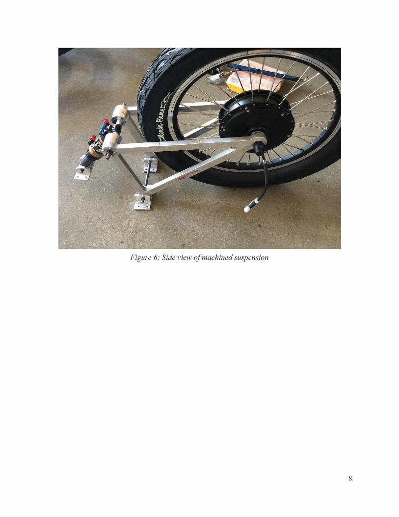
Figure 6: Side view of machined suspension

8

B. Testing

1. Experimental Setup

To assess the mechanical behavior of the suspension, our team setup an experiment

which involved securely fastening the suspension, statically deflecting it, and

dynamically releasing it (see fig. 7, 8, & 9 below). To begin, the base was secured to a

table with clamps (see figure 10 below). Next, a system was assembled to apply a

measurable force to deflect the suspension. Straps were tied to the base of the table

and looped around the edge in order to create an anchor point. The other end of the

strap was fed into a tensioner (see figure 11 below). The tensioner was attached to a

force gauge, which itself was attached to a mock axle in the suspension where the

wheel would otherwise be (see figure 12 below). Lastly, a potentiometer was attached

to the mock axle such that displacement could be measured (see figure 13 below).

With the experimental setup complete, a procedure was followed to document the

suspension’s static and dynamic characteristics. First an arduino data acquisition

program was run to begin collecting data from the potentiometer. Then the tensioner

was applied to slowly increase force applied to the suspension. After settling on an

appropriate maximum force, the force was recorded manually. Finally, the zip-ties

connecting the force gauge to the tensioner were rapidly severed to allow the

suspension to dynamically respond to a change in force. All of the displacement data

was recorded via the arduino program at 100 Hz. The analysis of this data can be

found in the next section of this report.

9

Figure 7: Overview of suspension experimental setup

Figure 8: Right-side view of experimental setup

10

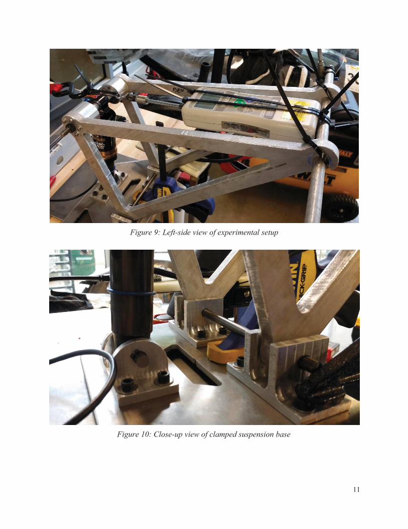
Figure 9: Left-side view of experimental setup

Figure 10: Close-up view of clamped suspension base

11

Figure 11: Strap tensioner for force application

Figures 12 & 13: Force gauge and potentiometer for data acquisition

12

2. Test Data

The analysis aspect of the suspensions testing was mainly focused on understanding

how the suspensions respond to varying compression forces at a given setting of its

inside pressure chambers. The suspension has two chambers: the upper one was varied

from 90 psi, 105 psi and 120 psi while the lower one was varied from 50 psi, 53 psi

and 58 psi. While these pressure values could be adjusted depending on the load, our

experiment focused on finding some optimal values of internal pressures that could be

relevant to the use of our urban concept vehicle, taking into consideration the weight

of the whole car and maximum weight of the two-seaters and their luggages. Through

this analysis, we will focus on finding the least amount of deflection for the greatest

amount of compression that the suspensions can possibly take. Ideally, we’re trying to

keep the suspensions displacement under 1 inch, for both structural support, damping

and safety reasons. Although this suspension testing doesn’t directly analyze the

optimum damping coefficient that’s desired for the suspensions, it certainly reveals

how much air pressure we should expect to put in the suspensions. Moreover, how

much displacement should be expected on the shock-absorbers when the car hits a

bump, carries heavy loads etc., which paves our analysis into further understanding

and research of the optimum damping coefficient.

Figure 14: A graph of suspension displacement versus time, taken when the

suspension was filled with a 90 psi on its upper chamber, and 50 psi on its lower

13

chamber. When subjected to different compression forces, the results are as shown

above. As expected, the force versus displacement response is steepest when the

suspension is compressed the most.

On Figure 14 above, we can see that at the 24.89 lbf of compression applied to the

suspensions, the maximum displacement effect due to that was 2.6496 inches. This

being about 2.6 times the desired displacement, it certainly means that the suspensions

need to be filled with more air pressure for a much higher damping ratio that would

result in less displacement.. At this applied force, the suspension constant, which is

equivalent to the spring constant, is 9.3939 lbf/in. Compared to spring constants of

78.7490 lbf/in, 36.0477 lbf/in and 18.9548 lbf/in for responses when the applied force

was much lesser (see Figure 14), it’s clear that we need a optimize between a higher

spring constant at any given load and the displacement response of the suspensions. So

far, we definitely need a suspension that can take more than 24.89 lbf without

displacing too much.




14



On Figure 15 above, we can see that at the 35.45 lbf of compression applied on the

suspension, the maximum displacement effect due to that was 4.5630 in. This being

about 4.6 times the maximum allowable displacement of 1 in, it certainly means that

the suspensions need to be filled with more air pressure for a much higher damping

ratio that would result in less displacement. At this applied force, the suspension

constant, which is equivalent to the spring constant, is 7.7690 lbf/in. Compared to

spring constants of 37.1413 lbf/in, and 19.1647 lbf/in for other responses when the

applied force was much lesser (see Figure 15), it’s clear that having more air pressure

in the suspension chambers has improved our results, but still the displacement

responses are too much for a higher load. We still need to optimize our variables for

better damping effects.






15

On Figure 16 above, we can see that at the 47.69 lbf of maximum compression applied

on the suspension, the maximum displacement effect due to that was 4.7548 in. This

being about 4.8 times the maximum allowable displacement of 1 in, it certainly means

that the suspensions need to be improved for a much higher damping ratio that would

result in less displacement and the maximum applied load possible. At this applied

force, the suspension constant is 10.0299 lbf/in. Compared to spring constants of

73.7295 lbf/in, and 24.8628 lbf/in for other responses when the applied force was

much lesser (see Figure 16), this implies that having more air pressure in the

suspension chambers has definitely improved our results, but displacement responses

are still too much for a higher load. At this point it has become clear that if we

pressurize the chamber high enough, we will get to a point where our desired loading

capacity is met with a lower displacement response. For now, a car suspension that

can’t take 47.69 lbf without displacing for more than an inch simply needs to be

improved. Pressuring the chambers further is definitely still possible at this point, until

the maximum allowable pressures in the chambers becomes our limiting factor. In that

case, our report would suggest much more powerful suspensions for the urban

concept.

Figure 17: The above graph puts all the graphs in Figure 14, 15 and 16 together for

comparison purposes. It’s apparent that pressurizing the chambers results into higher

16

spring constant values, which initially makes the suspensions to respond with a lesser

displacement for an applied static load. However, the more the load is applied, the

more pressure is required to sustain a relatively lower displacement on the

suspensions.

In summary, our observations on the suspension testing reveal that certainly pressuring

the upper and lower chambers increases the spring constant, as expected. While this

improves the damping ability on the suspensions, an optimal balance between air

pressure and applied force needs to be reached in order to determine which values of

allowable pressure and applied load will keep our displacement under 1 in. For the

given experimental method above, more variations of force may be applied on the

suspensions to see how much it can take for the most minimal displacement. Given the

limitations of our testing facilities in the workshop, more advanced testing equipments

are need in order to subject the suspension to more static and dynamic loads safely.

This could certainly not be done safely within our workshop.

17

C. MATLAB Calculations

All calculations below were written into a script and solved in MATLAB -- see Appendix

B for full code and results.

1. Resting Weight & Cornering

The mass of the car was found using the Mass Properties feature in Solidworks of the

full car assembly, including the body, suspension, ballast, wheels, one passenger, and

seats. An additional 30lbs were added to the number obtained to approximate the

weight of steering, seat belts, and other miscellaneous accessories that were not

included in the assembly. A simple force balance using a free body diagram of the car

was used to determine the amount of weight carried by each wheel: 68lbs for each

front wheel and 74lbs for each rear wheel. Cornering was similarly simplified, and the

forces going into each wheel were obtained by using the equation for centripetal force,

, and assuming each wheel carried 1/4 of the force with no slippage. TheF = rmV 2

magnitude of the force found, assumed to be acting perpendicularly to the front wheel

wells and in shear along the back wall, was 72lbs. These values were later used for

conducting a finite element analysis on the suspension and the body in Solidworks.

2. Braking

The forces going into the front and rear suspensions during braking were found using

two sets of force-balance equations: one on a free body diagram of the entire car, and

the other on a free body diagram of one side of the rear suspension. The first set of

equations considered the front two wheels grouped together and the rear two wheels

grouped together, and a deceleration in the x-direction was included in the force

balance under the assumption that braking would occur purely due to pure static

friction. The system of equations obtained were as follows (see Appendix C for

diagrams and derivations):

(F )tb

mv0 = σs y + Ry (1)

gm = Ry + F y (2)

y (R ) xσs c y + F y = F y c1 − Ry + xc2 (3)

where m was the total mass of the car, obtained from Solidworks, xc1, xc2, and yc were

the distances from the COG to the front axle, to the rear axle, and to the ground,

respectively, also obtained from Solidworks. σ s was the coefficient of static friction

between the tires and the road, assumed to be 1.2, and v0 was the running speed of the

car, assumed to be 25 mph.

18

Once tb, Rx, Ry, Fx, and Fy (time to brake, x and y components of the rear wheel forces,

and x and y components of the front wheel forces) were obtained in MATLAB, they

were plugged into the second set of equations to find the theoretical forces going into

the upper and lower pins of the rear suspension:

cosθS s + P x = Rx1 (4)

sinθS s − P y = − Ry1 (5)

y x (cosθ y inθ x )Rx1 r + Ry1 r = S s s − s s s (6)

where θ s was the angle between the ground and the rear shock (obtained from

Solidworks), S was the magnitude of the force being transmitted at angle θ s to the

upper pin in the suspension, Px, and Py were the x and y components of the force going

into the lower pin of the suspension, xR, xS, yR, and yS were the x and y distances from

the lower pin to the axle and the upper pin, respectively (obtained from Solidworks),

and Rx1 and Ry1 were the rear wheel reaction forces found above, divided by two to

obtain the effects on one wheel.

Once S, Px,, and Py were calculated in MATLAB, the results were plugged into the

beam bending stress equation ( ) and shear stress equation ( ) to obtain the σ =I

My τ = AF

maximum stresses in the pins. Since the lower pin experiences less force and is

significantly shorter than the upper pin, the upper pin was checked for failure in

bending and the lower pin was checked for failure in shear. The results for maximum

stress in the entire system, found in the upper pin, and the corresponding FOS for the

car in braking were found to be 26688.13 psi and 4.68, respectively.

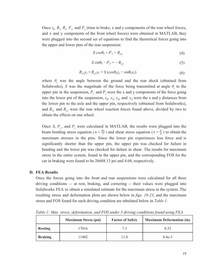
D. FEA Results

Once the forces going into the front and rear suspensions were calculated for all three

driving conditions -- at rest, braking, and cornering -- their values were plugged into

Solidworks FEA to obtain a simulated estimate for the maximum stress in the system. The

resulting stress and deformation plots are shown below in figs. 18-23, and the maximum

stress and FOS found for each driving condition are tabulated below in Table 1.

Table 1: Max. stress, deformation, and FOS under 3 driving conditions found using FEA

Maximum Stress (psi) Factor of Safety Maximum Deformation (in)

Resting 17016 7.3 0.32

Braking 11402 11.0 8.4e-3

19

Cornering 40954 3.1 0.13

1. Resting Weight

Figure 18: Stress plot for rear suspension under resting weight. Max stress = 17016 psi

Figure 19: Deformation plot for rear suspension under resting weight. Max deformation = 0.32”

20

2. Braking

Figure 20: Stress plot for rear suspension under braking forces. Max stress = 11402 psi

Figure 21: Deformation plot for rear suspension under braking forces.

Max deformation = 8.4e-3 in

21

3. Cornering

Figure 22: Stress plot for rear suspension under cornering forces. Max stress = 40954 psi

Figure 23: Deformation plot for rear suspension under cornering forces. Max deflection = 0.13”

22

III. Carbon Fiber and Honeycomb Testing

In order to obtain accurate results in a finite element analysis of the Urban Concept body, a

few properties of the composite material had to be experimentally established and loaded into

Solidworks. A mathematical relation was derived with the help of Dr. Knight (see Appendix

C) that relates the stresses found in a Solidworks model of the body -- which assumed a

completely uniform, homogenous material -- and the theoretical stresses found in the far

more complex composite material actually used. This information, along with the yield

strength determined during the break testing, provided a factor of safety for the entire car

body under various driving conditions.

A. Bending test procedure

To evaluate the optimal pairing of honeycomb and carbon fiber for the Urban Concept

body, a break test was conducted on eight sandwich panels constructed with different

combinations of honeycomb and carbon fiber. Three of the panels had two layers of 1/4”

thick honeycomb with two layers of carbon fiber on the outside and two layers in between,

another three panels had two layers of 1/4” thick honeycomb with three layers of carbon

fiber on the outside and two in between, and the last two panels had one layer of 1/2” thick

honeycomb with two layers of carbon fiber on the outside. Each panel was roughly 6”

wide by 12” long, and care was taken to ensure that their resin was fully and properly

cured.

For ease of analysis, the test was set up to simulate a two-dimensional, simply-supported

beam in bending with a point load in the center. A Tinius Olsen three-point bending

system in the Department of Civil Engineering lab was used to conduct the tests, which

had a maximum load capacity of 10,000 lbs and a digital output monitor for collecting

force vs. displacement data in real time. Because the panels were 6” wide, a thin

rectangular piece of steel was used to apply the load in a straight line across the width of

the specimen and simulate two dimensional bending conditions. The panels were placed

across two simple supports, and the distance between their centerlines was measured and

recorded as the span.

As each sample was slowly loaded with increasing force, the force and its corresponding

deflection were read off the output monitor and recorded in Excel for plotting and

analysis. The first sample was simply observed during the break test to watch its behavior,

and as a result, no data was taken. For the first few sample panels after that, data was only

collected up until the point of failure, and so the graphs for those panels only include the

linear portion of the force vs. deflection curve. The last few panels included the behavior

after failure, and the exact point of failure was recorded for all of the tests except one.

23

Figure 24: Bending test setup before applying load

Figure 25: Fully broken test specimen; failure due to delamination

24

B. Testing Data

The force and displacement data collected was plotted to find the Young’s Modulus for

each sample panel, examples of which can be found below in figs. 26-27 (see Appendix E

for all raw data).

Figure 26: Force vs. deflection plot for two-layer, 1/4” thick honeycomb sample

Figure 27: Force vs. deflection plot for one-layer, 1/2” thick honeycomb sample

By taking the slope of the linear portion of the plot and various dimensions of the

specimen, the Young’s Modulus was calculated using the beam deflection equation:

E = δF L

3

4bs3 (7)

Additionally, the yield stress was calculated from the yield strength found during the

break tests using the normal stress in beam bending equation:

25

σcr = 23

bs2

F Lcr (8)

The resulting average values for Young’s Modulus and yield stress are summarized in

Table 2 below, and were input as the material properties in Solidworks FEA to obtain

stress and deflection data for the car body.

Table 2: Average Young’s Moduli and yield stresses for each type of sandwich panel

2x0.25",

1+2-layer CF

2x0.25",

2-layer CF

2x0.25",

3-layer CF

1x0.5",

2-layer CF

Average Young’s

Modulus (psi) 491212.2 476236.7 429107.9 783449.3

Average yield

strength (psi) 3713.5 3393.5 3298.1 6550.0

C. FEA results

Using the values for the single-layer, 1/2” thick honeycomb as the input material

properties, as well as the estimated forces calculated in Section 2C above, the maximum

stress in the uniform material monocoque was found in Solidworks FEA for each of three

loading conditions: resting weight, braking, and cornering (see Table 3 below). Figs.

28-33 show heat maps for both stress and displacement under each of these conditions.

Table 3: Average Young’s Moduli and yield stresses for each type of sandwich panel

Maximum Stress

(uniform material) (psi) Maximum Deformation (in)

Resting 59.0 1.5e-2

Braking 58.9 1.65e-3

Cornering 145.8 8.4e-3

26

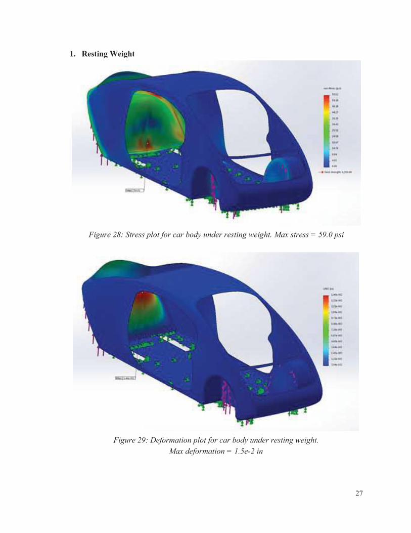
1. Resting Weight

Figure 28: Stress plot for car body under resting weight. Max stress = 59.0 psi

Figure 29: Deformation plot for car body under resting weight.


27

2. Braking

Figure 30: Stress plot for car body in braking forces. Max stress = 58.9 psi

Figure 31: Deformation plot for car body in braking forces.


28

3. Cornering

Figure 32: Stress plot for car body in cornering forces. Max stress = 145.8 psi

Figure 33: Deformation plot for car body in cornering forces.


29

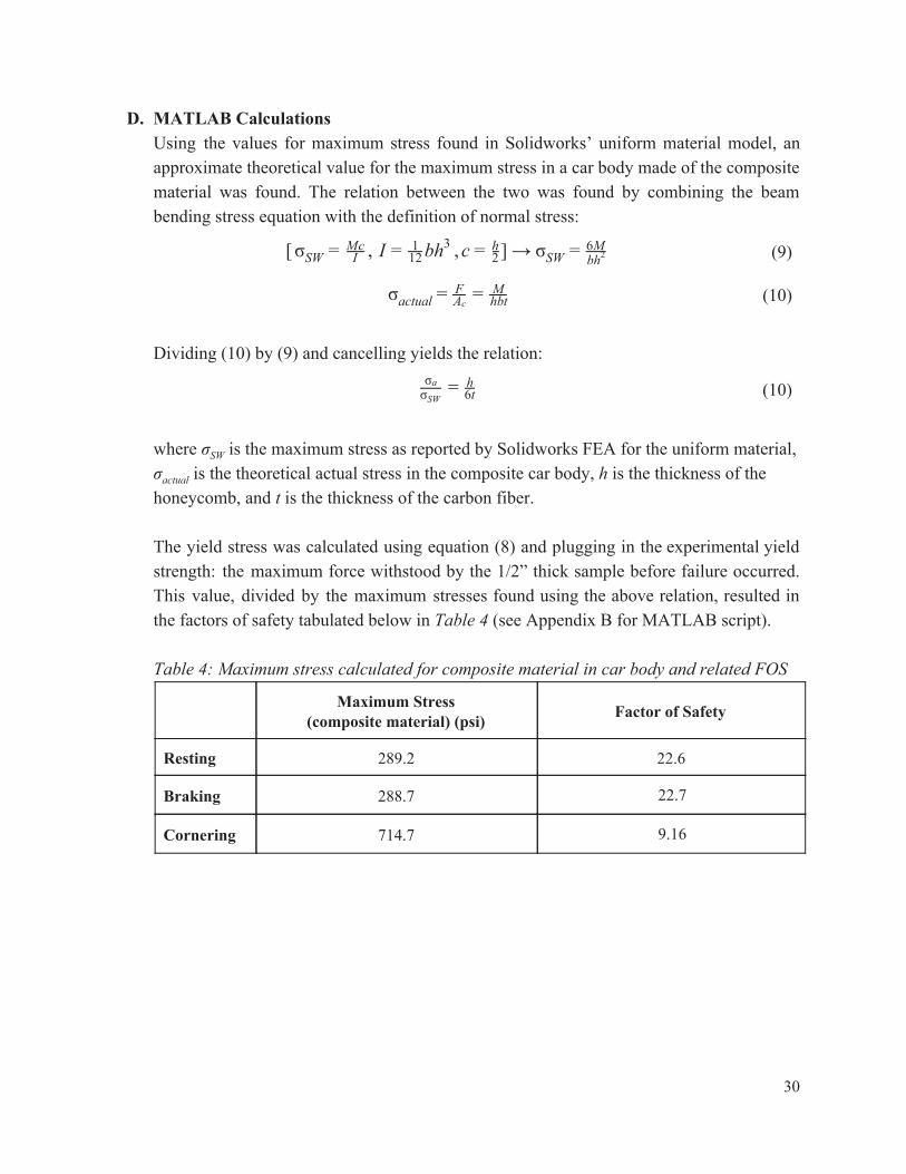
D. MATLAB Calculations

Using the values for maximum stress found in Solidworks’ uniform material model, an

approximate theoretical value for the maximum stress in a car body made of the composite

material was found. The relation between the two was found by combining the beam

bending stress equation with the definition of normal stress:

[ , , σSW = IMc bhI = 1

123

] c = 2h → σSW =

bh2

6M (9)

σactual = FAc

= Mhbt (10)

Dividing (10) by (9) and cancelling yields the relation:

σa

σSW= h

6t (10)

where σ SW is the maximum stress as reported by Solidworks FEA for the uniform material,

σ actual is the theoretical actual stress in the composite car body, h is the thickness of the

honeycomb, and t is the thickness of the carbon fiber.

The yield stress was calculated using equation (8) and plugging in the experimental yield

strength: the maximum force withstood by the 1/2” thick sample before failure occurred.

This value, divided by the maximum stresses found using the above relation, resulted in

the factors of safety tabulated below in Table 4 (see Appendix B for MATLAB script).

Table 4: Maximum stress calculated for composite material in car body and related FOS

Maximum Stress

(composite material) (psi) Factor of Safety

Resting 289.2 22.6

Braking 288.7 22.7

Cornering 714.7 9.16

30

IV. Conclusions and Future Modifications

In summary, the technical report of the Bass Connections Electric Vehicle Team

encompasses different aspects of building and testing the prototype. Different testing

methods were devised in order to evaluate our engineering decisions on the choice of

materials we used to build the body as well as the mechanical systems we designed for the

car. Our use of the carbon-fiber honeycomb materials to build the monocoque was validated

through a series of strength tests that were conducted on selected samples. The choice

between single layers of much thicker honeycomb material versus double layers of thinner

honeycomb materials was evaluated during strength testings and compared after a thorough

data analysis. The ½” thick honeycomb was most resistant to failures that would normally

result from delamination compared to the ¼” thick honeycomb samples. There was a slight

benefit to the double-layer 1/4” honeycomb; as the force on the samples increased, only one

of the two layers would delaminate at a time -- giving the user some audible feedback that

failure was occurring before both layers completely delaminated. However, the significantly

higher strength of the single-layer honeycomb would greatly outweigh the benefit of gradual

failure in the double-layer honeycomb, and in any case neither of those failures were

ultimate, as the carbon fiber had still been stretching without tearing when the tests were

ended. Several improvements could be implemented in the future, such as conducting more

extensive testing on different number of layers of carbon fiber honeycomb as well as

experimenting with many layers of just carbon fiber itself. Moreover, the team will have to

determine the best way to inlay the metal mounting plates if a single layer of honeycomb is

used instead of two, as the plate will protrude from the surface of the honeycomb and create

an uneven wall that is more at risk for delamination. Consideration can be given to adding a

layer of 1/4” thick honeycomb with the shape of the metal inlay cut out on top of the 1/2”

thick honeycomb for that purpose.

Another important part of the technical report is the FEA data and results. After having

decided which layer of honeycomb gave us the strongest and most durable structure, we

applied the ½” thick layer as the material for our prototype car and conducted an FEA on it in

SolidWorks under different driving conditions. Factors of safety were determined according

to each driving condition: the prototype car at rest would have a factor of safety of 22.6, 22.7

while braking, and 9.16 while cornering. As expected, the car would be subjected to

significantly higher stresses when cornering, almost twice as much as compared to the other

situations, as the forces are acting normal to the front wheel well walls, which have small

radii of curvature and therefore more locations of high stress concentration. Our analysis

methods did not allow us to account for delamination of the composite when shear stress was

applied and the software was generally limited in its capabilities; using a more sophisticated

31

FEA package or conducting further tests on the highly complex composite material would be

advisable for obtaining more accurate results in the future.

Furthermore, the suspension testing aspect of the project demonstrated that an optimal level

of pressure in both suspension chambers may be reached for a specified amount of load

going into the suspension. Our analysis has shown that the current suspensions can be

pressurized to much higher values to fit our needs. However, one of the main challenges we

experienced during the experiment was that achieving such levels may require the use of a

compressor instead of the hand pump used during experimentation. Subjecting such a highly

pressurized suspension to static and dynamic loads is extremely dangerous and therefore

requires much more sophisticated testing equipment and facilities. Another area of

improvement could be testing the suspension on a much more rigid jig frame than the one

built for this experiment. The front wheel suspensions would also have to be mounted on this

frame with steering and brakes to test rolling conditions in a more realistic environment.

Among others, the tests could also include obtain damping coefficient data when the

prototype is rolled over a bump, or the actual forces going into the suspension could be taken

under various driving conditions to make the FEA simulation more accurate.

Overall, the prototype comes with much promise for success and we look forward to seeing

its completion in the coming years. We hope the team will build upon our designs to make

the car lighter and more aerodynamic through refinement of the design and material choices

in order to directly improve our performance and efficiency -- as this was the team’s first

Urban Concept design, many parts may have been over-engineered and several changes can

be made to cut down on weight. With our distinguished advisors and Duke Electric Vehicle’s

steady hands, our hopes to paint the town while riding in this electric car are higher than

ever.

32

Appendix A: Rear Suspension CAD

Appendix B: MATLAB Script for Force Loads

% Anny Ning

% DEV senior design project

% Standard braking forces

clear; clc

%% Initialize variables

% Assume:

g = 32.2; % ft/s^2; acceleration due to gravity

sigma = 1.2; % coefficient of static friction b/w tires and ground

v0 = 25 * 5280/3600; % mph to fps; running speed of car

% Taken from SolidWorks:

m = (252.77+30)/g; % lbm to slugs, with 30 added lbs; mass of car + driver

xc1 = 41.8/12; % ft; dist from COG to center of front wheels

xc2 = 38.2/12; % ft; dist from COG to center of rear wheels

yc = 15.3/12; %ft; dist from COG to ground

%% System of equations to find braking forces

syms tb Ry Fy

eqn1 = sigma*(Fy+Ry) == m*v0/tb; % force balance in x dir; accel from braking

eqn2 = m*g == Ry + Fy; % force balance in y direction

eqn3 = sigma*yc*(Ry+Fy) == Fy*xc1 - Ry*xc2; % moment balance about COG

solution = solve([eqn1, eqn2, eqn3], [tb, Ry, Fy]);

tbSol = vpa(solution.tb, 6) % seconds; time required to brake

FySol = vpa(solution.Fy, 6); % lbf; force in y dir on both front wheels

RySol = vpa(solution.Ry, 6); % lbf; force in y dir on both rear wheels

FxSol = vpa(sigma*FySol, 6); % lbf; force in x dir on both front wheels

RxSol = vpa(sigma*RySol, 6); % lbf; force in x dir on both rear wheels

%% Braking forces, per wheel

Fx1 = vpa(FxSol/2, 5) % lbf; force in x dir on one front wheel

Fy1 = vpa(FySol/2, 5) % lbf; force in y dir on one front wheel

Rx1 = vpa(RxSol/2, 5) % lbf; force in x dir on one rear wheel

Ry1 = vpa(RySol/2, 5) % lbf; force in y dir on one rear wheel

%% Initialize variables


thetaS = 47.2; % degrees; angle b/w ground and rear shock

xR = 14.7/12; % in to ft; distance from lower pin to axle in x direction

yR = 1.88/12; % in to ft; distance from lower pin to axle in y direction

xS = 2.67/12; % in to ft; distance from upper pin to axle in x direction

yS = 7.63/12; % in to ft; distance from upper pin to axle in y direction

%% System of equations to find forces in rear suspension

syms Px Py S

eqn4 = S*cosd(thetaS) + Px == Rx1; % force balance in x direction

eqn5 = S*sind(thetaS) - Py == -Ry1; % force balance in y direction

eqn6 = Rx1*yR + Ry1*xR == S*(cosd(thetaS)*yS-sind(thetaS)*xS); % moment balance

solution2 = solve([eqn4, eqn5, eqn6], [Px, Py, S]);

Px1 = vpa(solution2.Px, 6) % lbf; forces on lower pin in x direction

Py1 = vpa(solution2.Py, 6) % lbf; forces on lower pin in y direction

S1 = vpa(solution2.S, 6) % lbf; force on upper pin at angle theta from ground

%% Max bending stress in upper pin

% Assume:

yieldstrength_pin = 125000; % psi; yield strength of 1144 steel from McMaster


L = 3.937; % in; length of shock pin between support collars

l1 = 0.498; % in; length of pin between collar and shock

l2 = 0.945; % in; width of shock

D = 0.3125; % in; diameter of pin

I = pi/64*D^4; % moment of inertia, circular cross-section

r = D/2; % radius of pin

M_max = (1/2)*S1*(l1+l2/4); % maximum bending moment in upper pin

max_stress_upperpin = vpa(M_max*r/I, 7) % psi; maximum bending stress in upper

pin

FOS_upperpin = vpa(yieldstrength_pin/max_stress_upperpin,3) % factor of safety

for upper pin

%% Max shear stress in lower pin

% Assume:

shearyieldstrength_pin = yieldstrength_pin*0.58; % psi; approx. shear yield

strength of 1144 steel

max_shearstress_lowerpin = vpa(sqrt(Px1^2+Py1^2)/(pi*r^2),6) % psi; maximum

shear stress in lower pin

FOS_lowerpin = vpa(shearyieldstrength_pin/max_shearstress_lowerpin,3) % factor

of safety for lower pin

%% Max stress in car body at rest

% Assume:

s = 0.5; % in; thickness of honeycomb, 1 layer of 0.5" thick

t = 0.017; % in; thickness of carbon fiber fabric

% Taken from SolidWorks FEA, for uniform material:

max_stress_SWcar_resting = 59; % psi; max stress in body at rest

max_stress_SWcar_braking = 58.9; % psi; max stress in body during braking

max_stress_SWcar_cornering = 145.8; % psi; max stress in body during cornering

% Taken from sample testing:

yieldstrength_car = 6550; % psi; critical stress for 1/2" honeycomb, from

testing data

max_stress_car_resting = vpa(max_stress_SWcar_resting*s/(6*t),6) % psi;

theoretical stress at rest

FOS_car_resting = vpa(yieldstrength_car/max_stress_car_resting,3) % factor of

safety at rest

max_stress_car_braking = vpa(max_stress_SWcar_braking*s/(6*t),6) % psi;

theoretical stress while braking

FOS_car_braking = vpa(yieldstrength_car/max_stress_car_braking,3) % factor of

safety while braking

max_stress_car_cornering = vpa(max_stress_SWcar_cornering*s/(6*t),6) % psi;

theoretical stress while cornering

FOS_car_cornering = vpa(yieldstrength_car/max_stress_car_cornering,3) % factor

of safety while cornering

MATLAB output:

tbSol =

0.94893

Fx1 =

119.95

Fy1 =

99.959

Rx1 =

49.711

Ry1 =

41.426

Px1 =

-98.2701

Py1 =

201.231

S1 =

217.798

max_stress_upperpin =

26688.13

FOS_upperpin =

4.68

max_shearstress_lowerpin =

2919.77

FOS_lowerpin =

24.8

max_stress_car_resting =

289.216

FOS_car_resting =

22.6

max_stress_car_braking =

288.725

FOS_car_braking =

22.7

max_stress_car_cornering =

714.706

FOS_car_cornering =

9.16

Appendix C: MATLAB Script for Suspension Tests

%% Abraham, Anny, Charlie

%% Import data from text file.

% Script for importing data from the following text file:

%

% /Users/abrahamnghwani/Documents/MATLAB/Suspension_data.csv

%

% To extend the code to different selected data or a different text file,

% generate a function instead of a script.

% Auto-generated by MATLAB on 2016/05/03 23:13:03

%% Initialize variables.

filename = '/Users/abrahamnghwani/Documents/MATLAB/Suspension_data.csv';

delimiter = ',';

%% Read columns of data as strings:

% For more information, see the TEXTSCAN documentation.

formatSpec = '%s%s%s%s%s%s%s%s%s%s%[^\n\r]';

%% Open the text file.

fileID = fopen(filename,'r');

%% Read columns of data according to format string.

% This call is based on the structure of the file used to generate this

% code. If an error occurs for a different file, try regenerating the code

% from the Import Tool.

dataArray = textscan(fileID, formatSpec, 'Delimiter', delimiter,

'ReturnOnError', false);

%% Close the text file.

fclose(fileID);

%% Convert the contents of columns containing numeric strings to numbers.

% Replace non-numeric strings with NaN.

raw = repmat({''},length(dataArray{1}),length(dataArray)-1);

for col=1:length(dataArray)-1

raw(1:length(dataArray{col}),col) = dataArray{col};

end

numericData = NaN(size(dataArray{1},1),size(dataArray,2));

for col=[1,2,3,4,5,6,7,8,9,10]

% Converts strings in the input cell array to numbers. Replaced

non-numeric

% strings with NaN.

rawData = dataArray{col};

for row=1:size(rawData, 1);

% Create a regular expression to detect and remove non-numeric prefixes

and

% suffixes.

regexstr =

'(?<prefix>.*?)(?<numbers>([-]*(\d+[\,]*)+[\.]{0,1}\d*[eEdD]{0,1}[-+]*\d*[i]{0,

1})|([-]*(\d+[\,]*)*[\.]{1,1}\d+[eEdD]{0,1}[-+]*\d*[i]{0,1}))(?<suffix>.*)';

try

result = regexp(rawData{row}, regexstr, 'names');

numbers = result.numbers;

% Detected commas in non-thousand locations.

invalidThousandsSeparator = false;

if any(numbers==',');

thousandsRegExp = '^\d+?(\,\d{3})*\.{0,1}\d*$';

if isempty(regexp(thousandsRegExp, ',', 'once'));

numbers = NaN;

invalidThousandsSeparator = true;

end

end

% Convert numeric strings to numbers.

if ~invalidThousandsSeparator;

numbers = textscan(strrep(numbers, ',', ''), '%f');

numericData(row, col) = numbers{1};

raw{row, col} = numbers{1};

end

catch me

end

end

end

%% Replace non-numeric cells with 0.0

R = cellfun(@(x) (~isnumeric(x) && ~islogical(x)) || isnan(x),raw); % Find

non-numeric cells

raw(R) = {0.0}; % Replace non-numeric cells

%% Create output variable

Suspensiondata = cell2mat(raw);

%% Clear temporary variables

clearvars filename delimiter formatSpec fileID dataArray ans raw col

numericData rawData row regexstr result numbers invalidThousandsSeparator

thousandsRegExp me R;

%% Creating the Variables

Suspensiondata([1 2 3],:)=[];

y1 = 0.007722.*Suspensiondata(:,1);










t1 = linspace(0,58.98,5898);

% Converting the applied force into a direct force applied at right angle

force = [25.4 36.7 41.1 43.1 41.7 51.5 61.4 61.3 71.4

82.6];

dir_force = force.*tan(13.09);

% Creating the data plots for each trial

figure(1);clf

plot(t1,y1,'k')

hold on

plot(t1,y2,'k-.')

plot(t1,y3,'k-*')

plot(t1,y4,'k-o')

plot(t1,y5,'b-')

plot(t1,y6,'b-.')

plot(t1,y7,'b-o')

plot(t1,y8,'g-')

plot(t1,y9,'g-.')

plot(t1,y10,'g-*')

title('A comparative plot of Displacement versus Time for all trials')

ylabel('Displacement (in)')

xlabel('Time (s)')

legend('Displacement at 90/50 psi with 14.67 lbf','Displacement at 90/50 psi

with 21.19 lbf','Displacement at 90/50 psi with 23.73 lbf','Displacement at

90/50 psi with 24.89 lbf','Displacement at 105/53 psi with 24.08

lbf','Displacement at 105/53 psi with 29.74 lbf','Displacement at 105/53 psi

with 35.45 lbf','Displacement at 120/58 psi with 35.39 lbf','Displacement at

120/58 psi with 41.23 lbf','Displacement at 120/58 psi with 47.69

lbf','Location','Southeast')

figure(2);clf

plot(t1,y1,'k')

hold on

plot(t1,y2,'b-.')

plot(t1,y3,'g-*')

plot(t1,y4,'c-o')

title('Displacement Vs Time for a 90/50 psi suspension, compressed by 14.67

lbf, 21.19 lbf, 23.73 lbf, and 24.89 lbf')


xlabel('Time (s)')

legend('Displacement at 90/50 psi with 14.67 lbf lbf','Displacement at 90/50

psi with 21.19 lbf lbf','Displacement at 90/50 psi with 23.73

lbf','Displacement at 90/50 psi with 24.89 lbf','Location','Southwest')

figure(3);clf

plot(t1,y5,'r')

hold on

plot(t1,y6,'b-.')

plot(t1,y7,'g-*')

title('Displacement Vs Time for a 105/53 psi suspension, compressed by a 24.08

lbf, 29.74 lbf, 35.45 lbf')


xlabel('Time (s)')


with 29.74 lbf','Displacement at 105/53 psi with 35.45

lbf','Location','Southwest')

figure(4);clf

plot(t1,y8,'m')

hold on

plot(t1,y9,'r-.')

plot(t1,y10,'g-*')

title('Displacement Vs Time for a 120/58 psi suspension, compressed by a 35.39

lbf,41.23 lbf,47.69 lbf')


xlabel('Time (s)')


with 41.23 lbf','Displacement at 120/58 psi with 47.69

lbf','Location','Southwest')

Appendix D: Derivation of Equations

Sample

# Outer

CF layers

Width

(b, in)

Honeycomb

thickness &

# layers

Thickness

(s, in)

Recorded

span (cm)

Span

(L, in)

Recorded

deflection (mm)

Deflection

(�, in)

Force

(F, lb)

Breaking strength

(F_cr, lb)

Yield strength

(psi)

Force/ Deflection

Slope (F/�) L^3/(4bs^3) E = (FL^3)/(4�bs^3) Notes

1 3 6 2x0.25in 0.5 23.2 9.13 5.7 0.224 230 283.6 2590.4 1024.9 254.0 260332.7

2 2 6 2x0.25in 0.5 24.0 9.45 0.2 0.008 10 282.5 2669.3 1536.8 281.2 432144.9

0.7 0.028 40

1.6 0.063 100

2.1 0.083 130

2.7 0.106 160

3.3 0.130 200

3.8 0.150 230

4.5 0.177 260

3 3 6 2x0.25in 0.5 24.0 9.45 0.5 0.020 20 337.2 3186.1 2077.6 281.2 584216.7

1.1 0.043 60

1.6 0.063 100

2.2 0.087 150

2.8 0.110 200

3.3 0.130 240

3.8 0.150 280

4.3 0.169 310

4 3 6 2x0.25in 0.5 24.0 9.45 0.5 0.020 20 435.8 4117.8 1574.6 281.2 442774.2

1.2 0.047 50

2.1 0.083 100

2.7 0.106 140

3.3 0.130 180

3.8 0.150 230

5.1 0.201 167

5.7 0.224 160

6.4 0.252 150

7.0 0.276 140

7.8 0.307 124

8.7 0.343 120

9.4 0.370 116

10.0 0.394 108

11.0 0.431 105

11.5 0.453 100

12.6 0.496 94

13.4 0.528 85

15.0 0.591 88

15.9 0.626 85

17.0 0.669 80

18.0 0.709 80

19.0 0.748 83

20.0 0.787 85

20.9 0.823 88

21.9 0.862 90

22.8 0.898 91

23.8 0.937 90

25.5 1.004 88

26.6 1.047 90

28.5 1.122 90

5 2 6 2x0.25in 0.5 24.0 9.45 0.5 0.020 10 435.8 4117.8 1850.4 281.2 520328.5

1.2 0.047 40

Only took data up to

breaking strength


breaking strength

Appendix E: Sample Testing Data

1.7 0.067 80

2.2 0.087 110

2.7 0.106 150

3.1 0.122 180

3.6 0.142 220

4.3 0.169 270

4.7 0.185 300

5.2 0.205 330

5.8 0.228 380

6.2 0.244 400

6.8 0.268 435

6 2 and 1 6 2x0.25in 0.5 25.2 9.92 0.5 0.020 20 374.3 3713.5 1509.0 325.5 491212.2

1.1 0.043 40

1.8 0.071 80

2.4 0.094 101

2.9 0.114 140

3.4 0.134 170

4.1 0.161 220

4.7 0.185 250

5.4 0.213 290

5.9 0.232 320

6.5 0.256 350

7.0 0.276 360

10.3 0.406 147

11.0 0.433 149

11.8 0.465 149

12.3 0.484 146

12.9 0.508 147

13.8 0.543 147

14.7 0.579 148

15.3 0.602 100

16.1 0.634 97

17.0 0.669 97

18.0 0.709 97

19.0 0.748 97

7 2 6 1x0.5in 0.5 25.2 9.92 0.5 0.020 15 - 2214.7 325.5 720932.9

0.9 0.035 25

1.8 0.071 50

2.3 0.091 80

2.7 0.106 110

3.2 0.126 150

3.6 0.142 190

4.1 0.161 230

4.5 0.177 270

5.0 0.197 310

5.4 0.213 350

5.9 0.232 390

6.6 0.260 450

7.1 0.280 490

7.7 0.303 505

8.2 0.323 530

8.8 0.346 540

9.2 0.362 550


breaking strength

Improperly laid outer

CF

kink in side

didn�t collect max

value so check

sample 8 results

9.9 0.390 290

10.8 0.425 290

11.4 0.449 290

12.6 0.496 290

13.3 0.524 280

14.0 0.551 281

14.8 0.583 282

15.6 0.614 278

16.7 0.657 276

17.6 0.693 263

18.6 0.732 250

19.6 0.772 251

20.6 0.811 248

21.4 0.843 245

22.5 0.886 242

23.5 0.925 240

8 2 6 2x0.5in 0.5 25.2 9.92 0.3 0.012 20 660.2 6550.0 2598.8 325.5 845965.7

0.8 0.031 50

1.2 0.047 90

1.6 0.063 130

2.1 0.083 180

2.5 0.098 220

2.9 0.114 270

3.5 0.138 320

3.8 0.150 370

4.6 0.181 430

5.1 0.201 490

5.5 0.217 530

6.6 0.260 630

7.3 0.287 190

7.9 0.311 220

8.5 0.335 228

9.4 0.370 225

10.1 0.398 228

11.0 0.433 234

11.6 0.457 232

12.6 0.496 227

13.5 0.531 227

14.5 0.571 224

15.2 0.598 216

16.0 0.630 216

17.2 0.677 210

18.3 0.720 202

19.0 0.748 200

19.8 0.780 200

20.7 0.815 200

21.6 0.850 201

22.6 0.890 199

23.8 0.937 197

24.8 0.976 195

25.8 1.016 190

26.8 1.055 190

2x0.25",

1+2-layer CF

2x0.25",

2-layer CF

2x0.25",

3-layer CF

1x0.5",

2-layer CF

491212.2 432144.9 260332.7 720932.9

520328.5 584216.7 845965.7

442774.2

Average: 491212.2 476236.7 429107.9 783449.3

3713.5 2669.3 2590.4 6550.0

4117.8 3186.1

4117.8

Average: 3713.5 3393.5 3298.1 6550.0

Young's

Moduli (psi)

Yield

strengths (psi)

y = 1536.8x + 0.139

R² = 0.9985

0

50

100

150

200

250

300

0.000 0.050 0.100 0.150 0.200

Fo

rce

(lb

s)

Deflection (in)

Sample #2, 2x0.25", 2-layer CF

y = 2077.6x - 30.095

R² = 0.9999

0

50

100

150

200

250

300

350

0.000 0.050 0.100 0.150 0.200

Fo

rce

(lb

s)

Deflection (in)


y = 1574.6x - 26.636

R² = 0.9976

0

50

100

150

200

250

0.000 0.200 0.400 0.600 0.800 1.000 1.200

Fo

rce

(lb

s)

Deflection (in)


y = 1850.4x - 45.909

R² = 0.9993

0

50

100

150

200

250

300

350

400

450

500

0.000 0.050 0.100 0.150 0.200 0.250 0.300

Forc

e (

lbs)

Deflection (in)


y = 1509x - 30.254

R² = 0.9971

0

50

100

150

200

250

300

350

400

0.000 0.100 0.200 0.300 0.400 0.500 0.600 0.700 0.800

Fo

rce

(lb

s)

Deflection (in)

Sample #6, 2x0.25", 2 & 1-layer CF

y = 2214.7x - 124.55

R² = 0.9995

0

100

200

300

400

500

600

0.000 0.200 0.400 0.600 0.800 1.000

Fo

rce

(lb

s)

Deflection (in)


y = 2598.8x - 32.521

R² = 0.9987

0

100

200

300

400

500

600

700

0.000 0.200 0.400 0.600 0.800 1.000 1.200

Fo

rce

(lb

s)

Deflection (in)
