United States Office of Water EPA-823-R00-012Environmental Protection 4305 July 2000Agency

BASINS Technical Note 6Estimating Hydrology and HydraulicParameters for HSPF

i

CONTENTS

Introduction . . . . . . . . . . . . . . . . . . . . . . . . . . . . . . . . . . . . . . . . . . . . . . . . . . . . . . . . . . . . . 1

Air Temperature (ATEMP) Parameters . . . . . . . . . . . . . . . . . . . . . . . . . . . . . . . . . . . . . . . . . 2

Snow (SNOW) Parameters . . . . . . . . . . . . . . . . . . . . . . . . . . . . . . . . . . . . . . . . . . . . . . . . . . . 3

Pervious Land Hydrology (PWATER) Parameters . . . . . . . . . . . . . . . . . . . . . . . . . . . . . . . . . 7

Impervious Land Hydrology (IWATER) Parameters . . . . . . . . . . . . . . . . . . . . . . . . . . . . . . . 18

Flow Routing (HYDR and ADCALC) Parameters . . . . . . . . . . . . . . . . . . . . . . . . . . . . . . . . 20

References . . . . . . . . . . . . . . . . . . . . . . . . . . . . . . . . . . . . . . . . . . . . . . . . . . . . . . . . . . . . . . 24

Parameter and Value Range Summary Tables . . . . . . . . . . . . . . . . . . . . . . . . . . . . . . . . . . . . 26

Page 1 of 32

BASINS Technical Note 6Estimating Hydrology and Hydraulic Parameters for HSPF

July, 2000

Introduction

This technical note provides BASINS users with guidance in how to estimate the input parametersin the ATEMP, SNOW, PWATER, IWATER, HYDR, and ADCALC sections of theHydrological Simulation Program Fortran (HSPF) watershed model. For each input parameter,this guidance includes a parameter definition, the units used in HSPF, and how the input valuemay be determined (e.g. initialize with reported values, estimate, measure, and/or calibrate). Where possible, the note discusses how to estimate initial values using the data and tools includedwith BASINS. Also discussed, where appropriate, is the physical basis of each parameter and thecorresponding algorithms as described in the HSPF Users Manual (Bicknell, et al, 1997) andearlier literature sources. In addition to the guidance provided below, model users are directed toother sources, including the ARM Model User Manual (Donigian and Davis, 1978), as well asstudies of agricultural BMP representation with HSPF (Donigian and Crawford, 1973;Donigian etal, 1983; and Casman, 1989).

Summary tables are attached that provide ‘typical’ and ‘possible’ (i.e. maximum ‘expected’)ranges for the parameters discussed below, based on both the parameter guidance and experiencewith HSPF over the past two decades on watersheds across the U. S. and abroad (Donigian,1998). The overarching principal in parameter estimation should be that the estimatedvalues must be realistic, i.e. make ‘physical’ sense, and must reflect conditions on thewatershed. If the values estimated by the model user and/or derived from the guidance below, donot agree with the value ranges in the summary table, the user should question and re-examine theestimation procedures. The estimated values may still be appropriate, but the user needs toconfirm that the parameter values reflect unusual conditions on the watershed.

Another source of parameter information is the HSPF Parameter Database (HSPFParm) (USEPA, 1999). Developed by AQUA TERRA Consultants, under contract to the EPA, HSPFParmconsists of parameter values from previous applications of HSPF across North Americaassimilated into a single database, and with a customized graphical user interface for viewing andexporting the data. The pilot HSPFParm Database contains parameter values for modelapplications in over 40 watersheds in 14 states. The parameter values, contained in the database,characterize a broad variety of physical settings, land use practices, and water quality constituents.The database has been provided with a simplified interactive interface that enables modelers toaccess and explore the HSPF parameter values developed and calibrated in various watershedsacross the United States, and to assess the relevance of the parameters to their own watershedsetting.

Page 2 of 32

The parameter guidance below is listed in order of the parameter tables required by each modulesection (i.e. ATEMP, SNOW, PWATER, IWATER, HYDR, and ADCALC) in the HSPF UCI(users control input) file, and the parameters are grouped as required in each UCI table.

Page 3 of 32

Air Temperature (ATEMP) Parameters

The ATEMP section variables are used by both the PERLND and IMPLND modules. Thissection is not required for basic hydrology unless SNOW is being simulated.

ATEMP-DAT Table:

ELDAT Elevation difference (feet), (measure). ELDAT is the difference in elevation betweenthe air temperature gage and the mean elevation of the associated pervious landsegment (PLS). ELDAT is equal to the PLS elevation minus the gage elevation andcan be either positive (PLS higher) or negative (gage elevation higher). ELDAT isused to adjust the gage air temperature to the PLS using a lapse rate; see Section4.2(1).1 in the HSPF User Manual (Bicknell et al., 1997) for additional information.

Use of BASINS Data/Tools:Weather station elevation is available in BASINS from the Elev_ft field in the WDMWeather Data Stations theme attribute table. To get the mean watershed elevation,run a Watershed Topographic Report. The mean elevation is available in theElevation Report.

AIRTMP Initial air temperature (degrees F), (measure/ estimate). Air temperature at start ofsimulation period.

Use of BASINS Data/Tools:Open the WDM file in WDM Utility (WDMUtil) and select the hourly air temperaturetime series (ATEM) for the weather station to be used in the simulation. Specify boththe current start and end dates as the model simulation start date and select an hourlytime step. Use the List/Edit Time Series function to display the air temperature for thestarting hour of the simulation.

Page 4 of 32

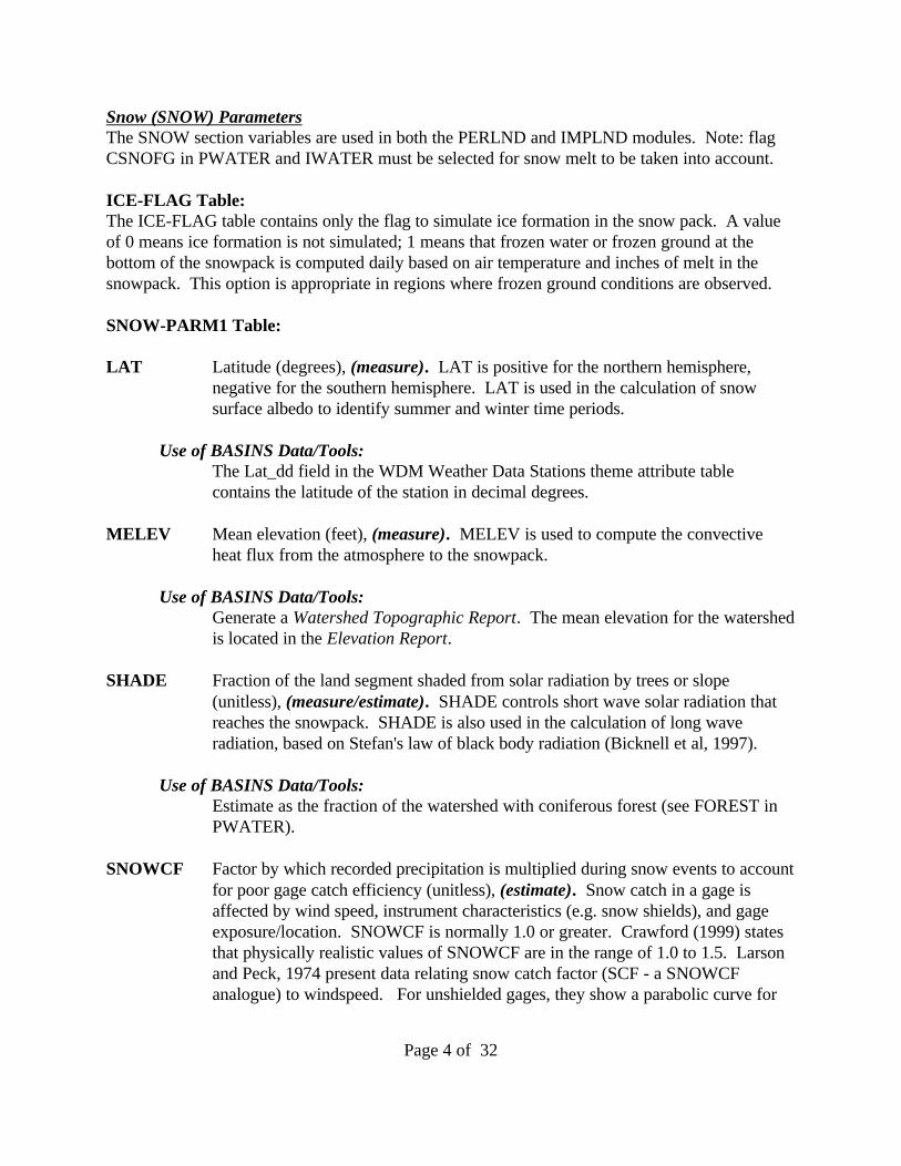
Snow (SNOW) ParametersThe SNOW section variables are used in both the PERLND and IMPLND modules. Note: flagCSNOFG in PWATER and IWATER must be selected for snow melt to be taken into account.

ICE-FLAG Table:The ICE-FLAG table contains only the flag to simulate ice formation in the snow pack. A valueof 0 means ice formation is not simulated; 1 means that frozen water or frozen ground at thebottom of the snowpack is computed daily based on air temperature and inches of melt in thesnowpack. This option is appropriate in regions where frozen ground conditions are observed.

SNOW-PARM1 Table:

LAT Latitude (degrees), (measure). LAT is positive for the northern hemisphere,negative for the southern hemisphere. LAT is used in the calculation of snowsurface albedo to identify summer and winter time periods.

Use of BASINS Data/Tools:The Lat_dd field in the WDM Weather Data Stations theme attribute tablecontains the latitude of the station in decimal degrees.

MELEV Mean elevation (feet), (measure). MELEV is used to compute the convectiveheat flux from the atmosphere to the snowpack.

Use of BASINS Data/Tools:Generate a Watershed Topographic Report. The mean elevation for the watershedis located in the Elevation Report.

SHADE Fraction of the land segment shaded from solar radiation by trees or slope(unitless), (measure/estimate). SHADE controls short wave solar radiation thatreaches the snowpack. SHADE is also used in the calculation of long waveradiation, based on Stefan's law of black body radiation (Bicknell et al, 1997).

Use of BASINS Data/Tools:Estimate as the fraction of the watershed with coniferous forest (see FOREST inPWATER).

SNOWCF Factor by which recorded precipitation is multiplied during snow events to accountfor poor gage catch efficiency (unitless), (estimate). Snow catch in a gage isaffected by wind speed, instrument characteristics (e.g. snow shields), and gageexposure/location. SNOWCF is normally 1.0 or greater. Crawford (1999) statesthat physically realistic values of SNOWCF are in the range of 1.0 to 1.5. Larsonand Peck, 1974 present data relating snow catch factor (SCF - a SNOWCFanalogue) to windspeed. For unshielded gages, they show a parabolic curve for

Page 5 of 32

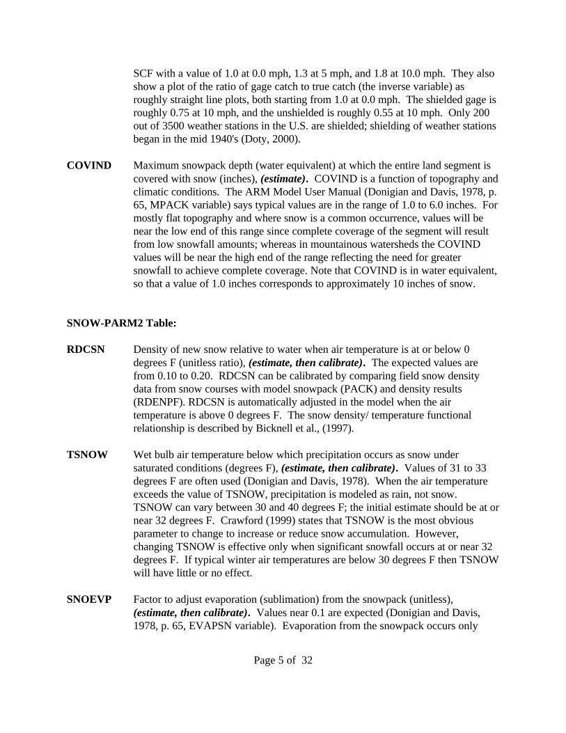
SCF with a value of 1.0 at 0.0 mph, 1.3 at 5 mph, and 1.8 at 10.0 mph. They alsoshow a plot of the ratio of gage catch to true catch (the inverse variable) asroughly straight line plots, both starting from 1.0 at 0.0 mph. The shielded gage isroughly 0.75 at 10 mph, and the unshielded is roughly 0.55 at 10 mph. Only 200out of 3500 weather stations in the U.S. are shielded; shielding of weather stationsbegan in the mid 1940's (Doty, 2000).

COVIND Maximum snowpack depth (water equivalent) at which the entire land segment iscovered with snow (inches), (estimate). COVIND is a function of topography andclimatic conditions. The ARM Model User Manual (Donigian and Davis, 1978, p.65, MPACK variable) says typical values are in the range of 1.0 to 6.0 inches. Formostly flat topography and where snow is a common occurrence, values will benear the low end of this range since complete coverage of the segment will resultfrom low snowfall amounts; whereas in mountainous watersheds the COVINDvalues will be near the high end of the range reflecting the need for greatersnowfall to achieve complete coverage. Note that COVIND is in water equivalent,so that a value of 1.0 inches corresponds to approximately 10 inches of snow.

SNOW-PARM2 Table:

RDCSN Density of new snow relative to water when air temperature is at or below 0degrees F (unitless ratio), (estimate, then calibrate). The expected values arefrom 0.10 to 0.20. RDCSN can be calibrated by comparing field snow densitydata from snow courses with model snowpack (PACK) and density results(RDENPF). RDCSN is automatically adjusted in the model when the airtemperature is above 0 degrees F. The snow density/ temperature functionalrelationship is described by Bicknell et al., (1997).

TSNOW Wet bulb air temperature below which precipitation occurs as snow undersaturated conditions (degrees F), (estimate, then calibrate). Values of 31 to 33degrees F are often used (Donigian and Davis, 1978). When the air temperatureexceeds the value of TSNOW, precipitation is modeled as rain, not snow. TSNOW can vary between 30 and 40 degrees F; the initial estimate should be at ornear 32 degrees F. Crawford (1999) states that TSNOW is the most obviousparameter to change to increase or reduce snow accumulation. However,changing TSNOW is effective only when significant snowfall occurs at or near 32degrees F. If typical winter air temperatures are below 30 degrees F then TSNOWwill have little or no effect.

SNOEVP Factor to adjust evaporation (sublimation) from the snowpack (unitless),(estimate, then calibrate). Values near 0.1 are expected (Donigian and Davis,1978, p. 65, EVAPSN variable). Evaporation from the snowpack occurs only

Page 6 of 32

when the vapor pressure of the air is less than that at the snow surface (Bicknell etal, 1997). Evaporation occurs only from the frozen content of the snowpack andis adjusted based on SNOEVP, wind movement, and the fraction of the landsegment covered by the snowpack. Snow evaporation is not large in mostwatersheds, but can be important where windy, low humidity conditions arecommon (Crawford, 1999).

CCFACT Factor to adjust the rate of heat transfer from the atmosphere to the snowpack,

due to condensation and convection, to match field conditions (unitless),(estimate, then calibrate). CCFACT is a function of climatic conditions. Typicalvalues are near 1.0, although a range of 0.5 to 2.0 has been observed (Donigianand Davis, 1978, p. 64, CCFAC variable). CCFACT is used in conjunction withwind movement and air temperature to compute heat transfer from the snowpackto the land surface.

MWATER Maximum liquid water holding capacity in the snowpack (in/in), (estimate, thencalibrate). MWATER is a function of the mass of ice layers; the size, shape, andspacing of snow crystals; and the degree of channelization and honeycombing ofthe snowpack to allow liquid water accumulation. Experimental values range from0.01 to 0.05, with 0.03 a common value (Donigian and Davis, 1978, p. 64, WC).

MGMELT Maximum rate of snowmelt by ground heat (in/day), (estimate, then calibrate). MGMELT is the rate of melt when the snowpack temperature is at 32 degrees F. A standard value is 0.01 in/day. Areas with deep frost penetration and/or frozenground have MGMELT values approaching zero (Donigian and Davis, 1978, p.64, DGM).

SNOW-INIT1 Table:

Pack-snow Initial quantity of snow (water equivalent) in the snowpack (inches), (estimate). Ifthe simulation starts at the beginning of the water year (October 1) Pack-snow isusually set to zero, except in arctic climates.

Pack-ice Initial quantity of ice (water equivalent) in the snowpack (inches), (estimate). Ifthe simulation starts at the beginning of the water year (October 1) Pack-ice isusually set to zero, except in arctic climates.

Pack-watr Initial quantity of liquid water in the snowpack (inches), (estimate). If thesimulation starts at the beginning of the water year (October 1) Pack-watr isusually set to zero, except in arctic climates.

Page 7 of 32

RDENPF Initial density of the frozen contents (Pack-snow and Pack-ice) of the snowpackrelative to water (unitless ratio), (estimate). If the simulation starts at thebeginning of the water year (October 1) RDENPF is usually set to 0.01 (minimumvalue), except in arctic climates; otherwise see RDCSN.

DULL Initial index to the dullness of the snowpack surface, from which the initial albedois estimated (unitless), (estimate). If the simulation starts at the beginning of thewater year (October 1) DULL is usually set to zero (for perfectly reflectablesnow), except in arctic climates. DULL ranges from zero to 800 and is anempirical index. It’s increased by one for each hour in which new snow does notfall.

PAKTMP Initial mean temperature of the frozen contents of the snowpack (degrees F),(estimate). If the simulation starts at the beginning of the water year (October 1)PAKTMP is usually set to 32 degrees F, except in arctic climates.

SNOW-INIT2 Table:

COVINX Initial snowpack depth (water equivalent) required for the entire land segment tobe covered with snow (inches), (estimate). If the simulation starts at the beginningof the water year (October 1) COVINX is usually set to its default value of 0.01,except in arctic climates; otherwise see COVIND, SNOW-PARM1.

XLNMLT Initial increment to ice storage in the snowpack (inches), (estimate). XLNMLTrepresents an equivalent heat deficit that must be overcome before snowmelt isreleased from the pack; otherwise some portion of the potential melt will freezeand become pack ice. For most simulations, XLNMLT can usually be set to zero,except possibly in arctic climates, because the values will be recalculated based oncurrent (usually hourly) air temperatures. XLNMLT is used only if ICE-FLAG isset to 1.

SKYCLR Initial fraction of sky assumed to be clear (unitless), (estimate). Unless a storm isin progress at the start of simulation period, set SKYCLR to 1.0 (no clouds).

Use of BASINS Data/Tools:Open the WDM file with the WDM Utility (WDMUtil) and select the CLOU timeseries for the weather station of interest. Identify the value of CLOU for thestarting date and time in the model simulation. Set SKYCLR to 1-CLOU.

Page 8 of 32

Pervious Land Hydrology (PWATER) Parameters

PWAT-PARM1 Table:The PWAT-PARM1 table includes flags to indicate the selected simulation algorithm option, orthe selection of monthly variability versus constant values for selected parameters. Where flagsindicate monthly variability, the corresponding monthly values must be provided in Monthly InputParameters (see below following the PWAT_PARM4 Table section). That section also providesguidance on which parameters are normally specified as monthly values.

CSNOFG Flag to use snow simulation data; must be checked (CSNOFG=1) if SNOW issimulated.

RTOPFG Flag to select overland flow routing method; choose either the method used inpredecessor models (HSPX, ARM, and NPS) or the alternative method asdescribed in the HSPF User Manual. Recommendation: Set RTOPFG=1; Thismethod, used in the predecessor models is more commonly used, and has beensubjected to more widespread application.

UZFG Flag to select upper zone inflow computation method; choose either the methodused in predecessor models (HSPX, ARM, and NPS) or the more exact numericalsolution to the integral of inflow to upper zone, i.e the alternative method. Recommendation: Set UZFG=1; This method, used in the predecessor models, ismore commonly used, and has been subjected to more widespread application.

VCSFG Flag to select constant or monthly-variable interception storage capacity, CEPSC. Monthly value can be varied to represent seasonal changes in foliage cover;monthly values are commonly used for agricultural, and sometimes deciduousforest land areas.

VUZFG Flag to select constant or monthly-variable upper zone nominal soil moisturestorage, UZSN. Monthly values are commonly used for agricultural areas toreflect the timing of cropping and tillage practices.

VMNFG Flag to select constant or monthly-variable Manning=s n for overland flow plane,NSUR. Monthly values are commonly used for agricultural, and sometimesdeciduous forest land areas.

VIFWFG Flag to select constant or monthly-variable interflow inflow parameter, INTFW. Monthly values are not often used.

VIRCFG Flag to select constant or monthly varied interflow recession parameter, IRC. Monthly values are not often used.

Page 9 of 32

VLEFG Flag to select constant or monthly varied lower zone ET parameter, LZETP. Monthly values are commonly used for agricultural, and sometimes deciduousforest land areas.

PWAT-PARM2 Table:

FOREST Fraction of land covered by forest (unitless) (measure/estimate). FOREST is thefraction of the land segment which is covered by forest which will continue totranspire in winter (i.e. coniferous). This is only relevant if snow is beingconsidered (i.e., CSNOFG=1 in PWATER-PARM1).

Use of BASINS Data/Tools:Run a Land Use Distribution Report on the watershed(s). Determine the acreagefor EVERGREEN FOREST LAND - 42. Estimate the fraction of MIXEDFOREST LAND - 43 acreage which is coniferous. Add this to the EVERGREENFOREST LAND - 42 acreage and divide the sum by the Forest land subtotalacreage. This is the value of FOREST for the Forested land use in that watershed. Estimate from field survey for all other land use types.

LZSN Lower zone nominal soil moisture storage (inches), (estimate, then calibrate). LZSN is related to both precipitation patterns and soil characteristics in the region. The ARM Model User Manual (Donigian and Davis, 1978, p. 56, LZSN variable)includes a mapping of calibrated LZSN values across the country based on almost60 applications of earlier models derived from the Stanford-based hydrologyalgorithms. LaRoche et al (1996) shows values of 5 inches to 14 inches, which isconsistent with the ‘possible’ range of 2 inches to 15 inches shown in the SummaryTable. Viessman, et al, 1989, provide initial estimates for LZSN in the StanfordWatershed Model (SWM-IV, predecessor model to HSPF) as one-quarter of themean annual rainfall plus four inches for arid and semiarid regions, or one-eighthannual mean rainfall plus 4 inches for coastal, humid, or subhumid climates. Theseformulae tend to give values somewhat higher than are typically seen as finalcalibrated values; since LZSN will be adjusted through calibration, initial estimatesobtained through these formulae may be reasonable starting values.

INFILT Index to mean soil infiltration rate (in/hr); (estimate, then calibrate). In HSPF,INFILT is the parameter that effectively controls the overall division of theavailable moisture from precipitation (after interception) into surface andsubsurface flow and storage components. Thus, high values of INFILT willproduce more water in the lower zone and groundwater, and result in higherbaseflow to the stream; low values of INFILT will produce more upper zone andinterflow storage water, and thus result in greater direct overland flow andinterflow. LaRoche et al (1996) shows a range of INFILT values used from 0.004

Page 10 of 32

in/hr to 0.23 in/hr, consistent with the ‘typical’ range of 0.01 to 0.25 in/hr in theSummary Table. Fontaine and Jacomino (1997) show sediment and sedimentassociated transport to be sensitive to the INFILT parameter since it controls theamount of direct overland flow transporting the sediment. Since INFILT is not amaximum rate nor an infiltration capacity term, it’s values are normally much lessthan published infiltration rates, percolation rates (from soil percolation tests), orpermeability rates from the literature. In any case, initial values are adjusted in thecalibration process.

INFILT is primarily a function of soil characteristics, and value ranges have beenrelated to SCS hydrologic soil groups (Donigian and Davis, 1978, p.61, variableINFIL) as follows:

SCS Hydrologic INFILT Estimate Soil Group (in/hr) (mm/hr) Runoff Potential

A 0.4 - 1.0 10.0 - 25.0 LowB 0.1 - 0.4 2.5 - 10.0 ModerateC 0.05 - 0.1 1.25 - 2.5 Moderate to HighD 0.01 - 0.05 0.25 - 1.25 High

An alternate estimation method that has not been validated, is derived from thepremise that the combination of infiltration and interflow in HSPF represents theinfiltration commonly modeled in the literature (e.g. Viessman et al, 1989, Chapter4). With this assumption, the value of 2.0*INFILT*INTFW should approximatethe average measured soil infiltration rate at saturation, or mean permeability.

Use of BASINS Data/Tools:Use of Soil Hydrologic Group/INFILT Table:Use the identify tool on the State Soil theme to identify the map unit identificationnumbers (Muid’s) for each soil layer overlapping the watershed. Open the SoilComponent Data table and perform a query for all records for each map unit (e.g.([Muid] = “PA044") or ([Muid] = “PA052") ) in the watershed. Highlight theHydgrp (soil hydrologic group) field and select summarize from the Table menu. Use the summary, together with the above table to estimate an average INFILTvalue for the watershed.

Use of Alternative 2.0*INFILT*INTFW Method:The State Soil (STATSGO) data layer contains data on soil permeability, definedin the 1996 National Soil Survey Handbook (Soil Survey Staff, 1996), as the rateof water movement through completely saturated soils. Run the BASINS StateSoil Characteristic Report and select mean estimate, area-weighted, surface layer,for permeability to get the value of 2*INFILT*INTFW. Note that although this

Page 11 of 32

method has not been validated, it may produce reasonable starting values foradjustment through calibration.

LSUR Length of assumed overland flow plane (ft) (estimate/measure). LSURapproximates the average length of travel for water to reach the stream reach, orany drainage path such as small streams, swales, ditches, etc. that quickly deliverthe water to the stream or waterbody. LSUR is often assumed to vary with slopesuch that flat slopes have larger LSUR values and vice versa; typical values rangefrom 200 feet to 500 feet for slopes ranging from 15% to 1 %. It is also oftenestimated from topographic data by dividing the watershed area by twice thelength of all streams, gullies, ditches, etc that move the water to the stream. Thatis, a representative straight-line reach with length, L, bisecting a representativesquare areal segment of the watershed, will produce two overland flow planes ofwidth ½ L. However, LSUR values derived from topographic data are often toolarge (i.e. overestimated) when the data is of insufficient resolution to display themany small streams and drainage ways. Users should make sure that valuescalculated from GIS or topographic data are consistent with the ranges shown inthe Summary Table.

Use of BASINS Data/Tools:Since RF3 data is not of sufficient resolution, use of this BASINS data layer is notrecommended for estimating LSUR.

SLSUR Average slope of assumed overland flow path (unitless) (estimate/measure). Average SLSUR values for each land use being simulated can often be estimateddirectly with GIS capabilities. Graphical techniques include imposing a gridpattern on the watershed and calculating slope values for each grid point for eachland use.

Use of BASINS Data/Tools:Within the BASINS GIS, identify DEM polygons, along the length of the reach(es)being modeled, which happen to be bisected by the reach. Adjacent, uphill DEMgrid cells, then, contain the elevation one grid cell away (i.e. 300 meters,measuring centerpoint to centerpoint). The approximate overland flow path slopeat that point in the reach is then the difference in elevation between the bisectedand the adjacent/uphill DEM grid cells, divided by the 300 meter (984 feet) widthof a grid cell. Make multiple estimates along the length of the reach(es) and usethese measurements to guide estimation of this parameter value.

KVARY Groundwater recession flow parameter used to describe non-linear groundwaterrecession rate (/inches) (initialize with reported values, then calibrate as needed). KVARY is usually one of the last PWATER parameters to be adjusted; it is usedwhen the observed groundwater recession demonstrates a seasonal variability with

Page 12 of 32

a faster recession (i.e. higher slope and lower AGWRC values) during wet periods,and the opposite during dry periods. LaRoche, et al, 1996 reported an extremelyhigh ‘optimized’ value of 0.66 mm-1 or (17 in-1) (much higher than any otherapplications) while Chen, et al, 1995 reported a calibrated value of 0.14 mm-1 (or3.6 in-1). Value ranges are shown in the Summary Table. Users should start with avalue of 0.0 for KVARY, and then adjust (i.e. increase) if seasonal variations areevident. Plotting daily flows with a logarithmic scale helps to elucidate the slopeof the flow recession.

AGWRC Groundwater recession rate, or ratio of current groundwater discharge to thatfrom 24 hours earlier (when KVARY is zero) (/day) (estimate, then calibrate). The overall watershed recession rate is a complex function of watershedconditions, including climate, topography, soils, and land use. Hydrographseparation techniques (see any hydrology or water resources textbook) can be usedto estimate the recession rate from observed daily flow data (such as plotting on alogarithmic scale, as noted above); estimated values will likely need to be adjustedthrough calibration. Value ranges are shown in the Summary Table. LaRoche, etal, 1996 reported an optimized value of 0.99; Chen, et al, 1995 reported valuesthat varied with land use type, ranging from 0.971 for grassland and clearings to0.996 for high density forest; Fontaine and Jacomino, 1997 reported a calibratedvalue of 0.99. This experience reflects normal practice of using higher values forforests than open, grassland, cropland and urban areas.

PWAT-PARM3 Table:

PETMAX Temperature below which ET will be reduced to 50% of that in the input timeseries (deg F), unless it=s been reduced to a lesser value from adjustments made inthe SNOW routine (where ET is reduced based on the percent areal snowcoverage and fraction of coniferous forest). PETMAX represents a temperaturethreshold where plant transpiration, which is part of ET, is reduced due to lowtemperatures (initialize with reported values, then calibrate as needed). It is onlyused if SNOW is being simulated because it requires air temperature as input (alsoa requirement of the SNOW module), and the required low temperatures willusually only occur in areas of frequent snowfall. Use the default of 40oF as aninitial value, which can be adjusted a few degrees if required.

PETMIN Temperature at and below which ET will be zero (deg F). PETMIN represents thetemperature threshold where plant transpiration is effectively suspended, i.e. set tozero, due to temperatures approaching freezing (initialize with reported values,then calibrate as needed). Like PETMAX, this parameter is used only if SNOWis being simulated because it requires air temperature as input (also a requirementof the SNOW module), and the required low temperatures will usually only occur

Page 13 of 32

in areas of frequent snowfall. Use the default of 35oF as an initial value, which canbe adjusted a few degrees if required.

INFEXP Exponent that determines how much a deviation from nominal lower zone storageaffects the infiltration rate (HSPF Manual, p. 60) (initialize with reported values,then calibrate as needed). Variations of the Stanford approach have used aPOWER variable for this parameter; various values of POWER are included inDonigian and Davis (1978, p. 58). However, the vast majority of HSPFapplications have used the default value of 2.0 for this exponent. Use the defaultvalue of 2.0, and adjust only if supported by local data and conditions.

INFILD Ratio of maximum and mean soil infiltration capacities (initialize with reportedvalue). In the Stanford approach, this parameter has always been set to 2.0, sothat the maximum infiltration rate is twice the mean (i.e. input) value; when HSPFwas developed, the INFILD parameter was included to allow investigation of thisassumption. However, there has been very little research to support using a valueother than 2.0. Use the default value of 2.0, and adjust only if supported by localdata and conditions.

Use of BASINS Data/Tools:Run the BASINS State Soil Characteristic Report and select mean estimate, area-weighted, surface layer, for permeability. The report lists the mean and maximumpermeability statistics by subwatershed. Use these values in conjunction with theguidance provided for INFILT.

DEEPFR The fraction of infiltrating water which is lost to deep aquifers (i.e. inactivegroundwater), with the remaining fraction (i.e. 1-DEEPFR) assigned to activegroundwater storage that contributes baseflow to the stream (estimate, thencalibrate). It is also used to represent any other losses that may not be measuredat the flow gage used for calibration, such as flow around or under the gage site. This accounts for one of only three major losses from the PWATER water balance(i.e. in addition to ET, and lateral and stream outflows). Watershed areas at highelevations, or in the upland portion of the watershed, are likely to lose more waterto deep groundwater (i.e. groundwater that does not discharge within the area ofthe watershed), than areas at lower elevations or closer to the gage (see discussionand figures in Freeze and Cherry, 1979, section 6.1). DEEPFR should be set to0.0 initially or estimated based on groundwater studies, and then calibrated, inconjunction with adjustments to ET parameters, to achieve a satisfactory annualwater balance.

BASETP ET by riparian vegetation as active groundwater enters streambed; specified as afraction of potential ET, which is fulfilled only as outflow exists (estimate, thencalibrate). Typical and possible value ranges are shown in the Summary Table. If

Page 14 of 32

significant riparian vegetation is present in the watershed then non-zero values ofBASETP should be used. Adjustments to BASETP will be visible in changes inthe low-flow simulation, and will effect the annual water balance. If riparianvegetation is significant, start with a BASETP value of 0.03 and adjust to obtain areasonable low-flow simulation in conjunction with a satisfactory annual waterbalance.

AGWETP Fraction of model segment (i.e. pervious land segment) that is subject to directevaporation from groundwater storage, e.g. wetlands or marsh areas, where thegroundwater surface is at or near the land surface, or in areas with phreatophyticvegetation drawing directly from groundwater. This is represented in the model asthe fraction of remaining potential ET (i.e. after base ET, interception ET, andupper zone ET are satisfied), that can be met from active groundwater storage(estimate, then calibrate). If wetlands are represented as a separate PLS(pervious land segment), then AGWETP should be 0.0 for all other land uses, anda high value (0.3 to 0.7) should be used for the wetlands PLS. If wetlands are notseparated out as a PLS, identify the fraction of the model segment that meets theconditions of wetlands/marshes or phreatophytic vegetation and use that fractionfor an initial value of AGWETP. Like BASETP, adjustments to AGWETP will bevisible in changes in the low-flow simulation, and will effect the annual waterbalance. Follow above guidance for an initial value of AGWETP, and then adjustto obtain a reasonable low-flow simulation in conjunction with a satisfactoryannual water balance.

PWAT_PARM4 Table:

CEPSC Amount of rainfall, in inches, which is retained by vegetation, never reaches theland surface, and is eventually evaporated (estimate, then calibrate). Typicalguidance for CEPSC for selected land surfaces is provided in Donigian and Davis(1978, p. 54, variable EPXM) as follows:

Land Cover Maximum Interception (in)Grassland 0.10Cropland 0.10 - 0.25Forest Cover, light 0.15Forest Cover, heavy 0.20

Donigian et al (1983) provide more detail guidance for agricultural conditions,including residue cover for agricultural BMPs. As part of an annual waterbalance, Viessman, et al. 1989 note that 10-20% of precipitation during growingseason is intercepted and as much as 25% of total annual precipitation isintercepted under dense closed forest stands; crops and grasses exhibit a wide

Page 15 of 32

range of interception rates - between 7% and 60% of total rainfall. Users shouldcompare the annual interception evaporation (CEPE) with the total rainfallavailable (PREC in the WDM file), and then adjust the CEPSC values accordingly. (See Monthly Input Values below).

UZSN Nominal upper zone soil moisture storage (inches) (estimate, then calibrate). UZSN is related to land surface characteristics, topography, and LZSN. Foragricultural conditions, tillage and other practices, UZSN may change over thecourse of the growing season. Increasing UZSN value increases the amount ofwater retained in the upper zone and available for ET, and thereby decreases thedynamic behavior of the surface and reduces direct overland flow; decreasingUZSN has the opposite effect. Donigian and Davis (1978, p. 54) provide initialestimates for UZSN as 0.06 of LZSN, for steep slopes, limited vegetation, lowdepression storage; 0.08 LZSN for moderate slopes, moderate vegetation, andmoderate depression storage; 0.14 LZSN for heavy vegetal or forest cover, soilssubject to cracking, high depression storage, very mild slopes. Donigian et al.,(1983) include detailed guidance for UZSN for agricultural conditions. LaRocheshows values ranging from 0.016 in to 0.75 in. Fontaine and Jacomino showedaverage daily stream flow was relatively insensitive to this value but sediment andsediment associated contaminant outflow was sensitive; this is consistent withexperience with UZSN having an impact on direct overland flow, but little impacton the annual water balance (except for extremely small watersheds with nobaseflow). Typical and possible value ranges are shown in the Summary Table.

NSUR Manning’s n for overland flow plane (estimate). Manning=s n values for overlandflow are considerably higher than the more common published values for flowthrough a channel, where values range from a low of about 0.011 for smoothconcrete, to as high as 0.050-0.1 for flow through unmaintained channels (Hwangand Hita, 1987). Donigian and Davis (1978, p. 61, variable NN) and Donigian etal (1983) have tabulated the following values for different land surface conditions:

Smooth packed surface 0.05Normal roads and parking lots 0.10Disturbed land surfaces 0.15 - 0.25Moderate turf/pasture 0.20 - 0.30Heavy turf, forest litter 0.30 - 0.45

Agricultural Conditions Conventional Tillage 0.15 - 0.25 Smooth fallow 0.15 - 0.20 Rough fallow, cultivated 0.20 - 0.30 Crop residues 0.25 - 0.35 Meadow, heavy turf 0.30 - 0.40

Page 16 of 32

For agricultural conditions, monthly values are often used to reflect the seasonalchanges in land surfaces conditions depending on cropping and tillage practices. Additional tabulations of Manning’s n values for different types of surface covercan be found in: Weltz, et al, 1992; Engman, 1986; and Mays, 1999. Manning’s nvalues are not often calibrated since they have a relatively small impact on bothpeak flows and volumes as long as they are within the normal ranges shown above. Also, calibration requires data on just overland flow from very small watersheds,which is not normally available except at research plots and possibly urban sites.

INTFW Coefficient that determines the amount of water which enters the ground fromsurface detention storage and becomes interflow, as opposed to direct overlandflow and upper zone storage (estimate, then calibrate). Interflow can have animportant influence on storm hydrographs, particularly when vertical percolation isretarded by a shallow, less permeable soil layer. INTFW affects the timing ofrunoff by effecting the division of water between interflow and surface processes. Increasing INTFW increases the amount of interflow and decreases direct overlandflow, thereby reducing peak flows while maintaining the same volume. Thus itaffects the shape of the hydrograph, by shifting and delaying the flow to later intime. Likewise, decreasing INTFW has the opposite effect. Base flow is notaffected by INTFW. Rather, once total storm volumes are calibrated, INTFW canbe used to raise or lower the peaks to better match the observed hydrograph. Typical and possible value ranges are shown in the Summary Table.

IRC Interflow recession coefficient (estimate, then calibrate). IRC is analogous to thegroundwater recession parameter, AGWRC, i.e. it is the ratio of the current dailyinterflow discharge to the interflow discharge on the previous day. WhereasINTFW affects the volume of interflow, IRC affects the rate at which interflow isdischarged from storage. Thus it also affects the hydrograph shape in the ‘falling’or recession region of the curve between the peak storm flow and baseflow. Themaximum value range is 0.3 – 0.85, with lower values on steeper slopes; valuesnear the high end of the range will make interflow behave more like baseflow,while low values will make interflow behave more like overland flow. IRC shouldbe adjusted based on whether simulated storm peaks recede faster/slower thanmeasured, once AGWRC has been calibrated. Typical and possible value rangesare shown in the Summary Table.

Page 17 of 32

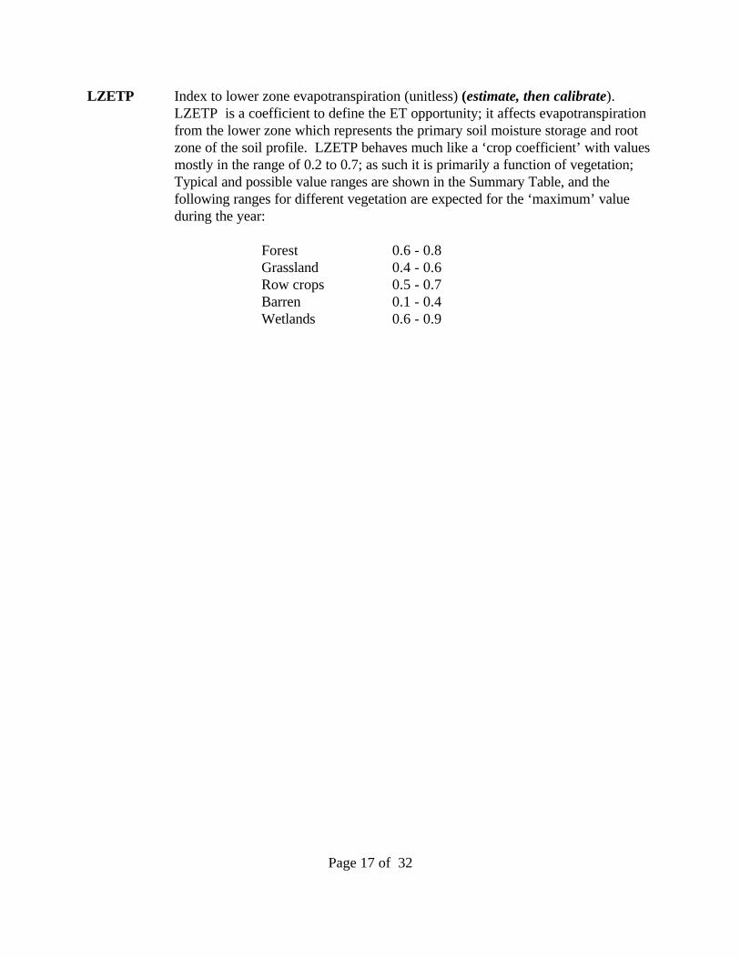
LZETP Index to lower zone evapotranspiration (unitless) (estimate, then calibrate). LZETP is a coefficient to define the ET opportunity; it affects evapotranspirationfrom the lower zone which represents the primary soil moisture storage and rootzone of the soil profile. LZETP behaves much like a ‘crop coefficient’ with valuesmostly in the range of 0.2 to 0.7; as such it is primarily a function of vegetation;Typical and possible value ranges are shown in the Summary Table, and thefollowing ranges for different vegetation are expected for the ‘maximum’ valueduring the year:

Forest 0.6 - 0.8Grassland 0.4 - 0.6Row crops 0.5 - 0.7Barren 0.1 - 0.4Wetlands 0.6 - 0.9

Page 18 of 32

Monthly Input Parameter Tables: In general, monthly variation in selected parameters, such as CEPSC and LZETP should beincluded with the initial parameter estimates. However, adjustments to the monthly values shouldbe addressed only after annual flow volumes are matched well with monitored data. All monthlyvalues can be adjusted to calibrate for seasonal variations.

MON-INTERCEP Table: Monthly values for interception storage. Monthly values can be developed based on the datapresented in the discussion in PWAT-PARM4/CEPSC and the Summary Tables.

MON-UZSN Table:Monthly values for upper zone storage. For agricultural areas under conventional tillage, lowervalues are used to reflect seedbed preparation in the spring with values increasing during thegrowing season until harvest and fall tillage. See PWAT-PARM4/UZSN discussion and SummaryTables for guidance.

MON-MANNING Table:Monthly values for Manning=s n for the overland flow plane. Monthly values can be used torepresent seasonal variability in ground cover including crop and litter residue. See discussion inPWAT-PARM4/NSUR for Manning’s n as a function of agricultural conditions.

MON-INTERFLW Table:Monthly values for interflow parameter (INTFW) are not often used.

MON-IRC Table:Monthly values for interflow recession parameter are not often used.

MON-LZETPARM Table:Monthly values for LZETP for evapotranspiration from the lower zone can be developed using anexpected maximum value from the PWAT-PARM4/LZETP discussion and the range of valuespresented in the Summary Tables. Monthly variable values should be used to reflect theseasonality of evapotranspiration, in response to changes in density of vegetation, depth of rootzone, and stage of plant growth.

Page 19 of 32

PWAT-STATE1 Table:CEPS, SURS, IFWS, UZS, LZS, AGWS, are initial values for storage of water in interception,surface ponding, interflow, the upper zone, lower zone, and active groundwater, respectively, andGWVS is the initial index to groundwater slope. All these storages pertain to the first interval ofthe simulation period.

The surface related storages (i.e. CEPS, SURS, IFWS) are highly dynamic, and will reach adynamic equilibrium within a few days, at most. These state variables can be left blank, or set to0.0 unless an individual storm is being simulated. The soil storages (i.e. UZS, LZS, and AGWS,and the GWVS) are much less dynamic, so their beginning values can impact the simulation for aperiod of months to a few years. If possible, users should allow as long a startup time period aspossible (i.e. set the simulation period to begin prior to the period you=ll use for comparisonagainst monitoring data or other use); as noted each of these storages should reach a dynamicequilibrium within a few years of simulation. UZS and LZS should be set equal to UZSN andLZSN respectively, unless it is known that the starting date is during a particularly wet or dryperiod; starting values can be increased or decreased if wet or dry conditions were evident priorto the simulation period. AGWS is a bit more problematic. If far too high or too low, baseflowwill be excessive or skewed low for several months or years, depending on AGWRC andKVARY. Improper values of GWVS can also cause simulation accuracy problems again forlengths of time depending on values of AGWRC and KVARY. However, since when KVARY isset to 0.0 seasonal recession is not represented and GWVS is not calculated. To avoid problems,then, AGWS should be set to 1.0 inch and GWVS to 0.0 for initial simulation runs.

If the simulation period is limited in duration, you can check and reset these state variables tovalues observed for the same period in subsequent years with similar climatic conditions. However, if major calibration changes are made to the parameters controlling these storages (e.g.UZSN, LZSN, INFILT), then the initial conditions should be checked and adjusted during thecalibration process. The values for AGWS and GWVS should be checked and adjusted as notedabove, which assuming a yearly cycle of groundwater storage, can be compared to values duringsimilar seasons in the simulation period. If the initial simulated baseflow (before the firstsignificant rainfall) is much different from the initial observed streamflow, then further adjustmentscan be made to raise or lower the flow rates.

Page 20 of 32

Impervious Land Hydrology (IWATER) Parameters

IWAT-PARM1 Table:The IWAT-PARM1 table includes a number of flag variables to indicate either the selection of asimulation algorithm option, or whether the parameter will be treated as a constant or be variedmonthly. As with PWAT-PARM1, where flags indicate monthly variability, correspondingmonthly values must be provided in Monthly Input Parameter tables (see below following IWAT-PARM3 section).

CSNOFG Flag to use snow simulation data; must be checked (CSNOFG=1) if SNOWmodule is run.

RTOPFG Flag to select overland flow routing method. If RTOPFG=0, a new routing

algorithm is used. RTOPFG=1 results in the use of the method used bypredecessor models (HSPX, ARM, and NPS). Recommendation: set RTOPFG=1;this method is more commonly used and has been subjected to more widespreadapplication.

VRSFG Flag to select constant or monthly-variable retention storage capacity, RETSC.Monthly values are not often used.

VNNFG Flag to select constant or monthly-variable Manning's n for overland flow plane,NSUR. Monthly values are not often used.

RTLIFG Flag to determine if lateral surface inflow to the impervious land segment will besubject to retention storage (RTLIFG=1). This flag only has an impact if theanother land segment drains to the impervious land segment; otherwise lateralsurface inflow is nonexistent. This feature is not commonly used in most HSPFapplications.

IWAT-PARM2 Table:

LSUR Length of assumed overland flow plane (feet), (measure/estimate). See PWAT-PARM2/ LSUR discussion. For impervious areas, LSUR reflects the overlandflow length on directly connected, or effective impervious area (EIA), and isusually in the range of 50 to 150 feet, although longer lengths may apply incommercial or industrial regions of large metropolitan areas. Impervious surfacesthat drain to pervious land, rather than to a reach, are considered part of thepervious land segment and not part of the EIA.

SLSUR Average slope of the assumed overland flow path (unitless), (measure/estimate). See PWAT-PARM2 / SLSUR discussion.

Page 21 of 32

NSUR Manning's n for overland flow plane (estimate). See PWAT-PARM4 / NSURdiscussion. Recommendation: set NSUR within the range of 0.05 to 0.10 forpaved roads and parking lots.

RETSC Retention (interception) storage of the impervious surface (inches) (estimate). RETSC is the impervious equivalent to the interception storage variable (CEPSC)used for pervious land segments. RETSC is the depth of water that collects on theimpervious surface before any runoff occurs. A study of five urban watersheds inthe Puget Sound region conducted by the U.S. Geological Survey (Dinicola, 1990)found that a value of 0.10 for RETSC was appropriate. If parking lots androoftops are designed for detention storage, larger values up to 0.5 inches may bereasonable.

IWAT-PARM3 Table:

The following two parameters are used only if SNOW is being simulated.

PETMAX Temperature below which ET will be reduced by 50% of that in the input timeseries (degree F), (estimate, then calibrate). See PWAT-PARM3 /PETMAXdiscussion.

PETMIN Temperature at and below which ET will be set to zero (degree F), (estimate, thencalibrate). See PWAT-PARM3 /PETMIN discussion.

Page 22 of 32

Monthly Input Parameter Tables:

MON-RETN Table:Monthly values for retention storage. Monthly values can be varied to represent seasonal changesin surface retention storage due to litter accumulation or sediment deposition on the impervioussurface. Monthly values are not often used.

MON-MANNING Table:Monthly values for Manning's n for the overland flow plane. As described above for MON-RETN, monthly values can be changed to represent seasonal changes on the surface of theimpervious area. Monthly values are not often used.

IWAT-STATE1 Table:RETS and SURS are initial values for storage of water in retention and surface ponding,respectively. Both of these storages pertain to the first day of the simulation period. RETS andSURS are highly dynamic and are only non-zero if the simulation starts during or just following astorm event. They can be left blank or set to zero unless an individual storm is being simulated.

Page 23 of 32

Flow Routing (HYDR and ADCALC) Parameters

HSPF computes streamflow through a stream reach or reservoir based on two assumptions: (1)there is a fixed relationship between depth, volume, and discharge, and (2) discharge is a functionof volume (see ODGTFG discussion for exception). This means that flow reversals andbackwater effects in an upstream reach are not simulated. Routing is computed using storagerouting or kinematic wave routing. Momentum is not considered in the routing computations.

HYDR-PARM1 Table:

The HYDR-PARM1 table includes flags to indicate which auxiliary variables to compute andinclude in the RCHRES printout as well as flags to select routing options based on either volume,time, or both. The auxiliary variables can be output to the WDM and statistically analyzed likeother time series.

VCONFG Flag to select constant or monthly-variable factors to adjust the outflow from theFTABLE discharge column, i.e. use the MON-CONVF table. Monthly values arenot often used.

AUX1FG Flag to compute stream channel depth, stage, surface area, average depth(volume/surface area), top width (surface area/length), and hydraulic radius. AUX1FG must be set to 1 if precipitation and evaporation fluxes are calculated forthe stream reach, or water quality is simulated for the reach.

AUX2FG Flag to compute average cross section area (volume/length) and average velocity(discharge/average cross sectional area). AUX2FG must be set to 1 if oxygen inthe stream reach is simulated. If AUX2FG=1 then AUX1FG must equal 1.

AUX3FG Flag to compute bed shear velocity and bed shear stress. These values are used tocalculate sediment deposition and scour (inorganic and organic) for a stream reach. If AUX3FG=1 then AUX2FG and AUX1FG must equal 1.

ODFVFG For use when the stream reach outflow demand is a function of volume. The valueis the column in the appropriate FTABLE that contains stream reach dischargevalues. A maximum of five discharge exits can be specified for a single streamreach. For a stream reach with a single exit, the appropriate value of ODFVFG(1)is usually 4, since the FTABLE includes columns for depth, surface area, andvolume in columns 1, 2, and 3, respectively. With two exits (e.g. natural exit plusa side diversion) ODFVFG(1)=4 and ODFVFG(2)=5.

If the value of ODFVFG is less than zero, then the absolute value is the column inthe COLIND time series which designates which FTABLE column to use. TheCOLIND time series is used to vary the FTABLE column used in the computation

Page 24 of 32

of discharge on a seasonal or daily basis. For example, if ODFVFG=-1 then themodel checks the appropriate COLIND value for that time step and if theCOLIND value equals 6 then column 6 in the FTABLE is used in the outflowcalculations for that particular stream reach. In addition, a fractional value forCOLIND can be used to interpolate between columns in the FTABLE, e.g. a valueof 4.3 can be used to interpolate between columns 4 and 5, with 30% of thedifference between columns 4 and 5 being added to column 4. This option can beused to simulate different rule curves and to vary from one set to another.

ODGTFG Flag to specify that the stream reach outflow demand is a function of time. Thevalue is the number corresponding to the OUTDGT subscript number specified inthe External Sources Block. The OUTDGT number links the reach outflowdemand to a flow time series data set in the WDM. A maximum of five dischargeexits can be specified for a single stream reach. For a stream reach with a singleexit, the appropriate value of ODGTFG(1) is usually 1 (the correspondingoperation number of OUTDGT in External Sources will then be 1). With twoexits (e.g. natural exit plus a side diversion) ODFVFG(1)=1 and ODFVFG(2)=2,corresponding to subscripts 1 and 2 of OUTDGT.

FUNCT Flag to combine ODFVFG and ODGTFG functions, if appropriate. For each of amaximum of 5 possible exits the value of FUNCT can be 1 (select the smaller ofthe ODFVFG and ODGTFG values), 2 (larger of ODFVFG and ODGTFG), or 3(sum of ODFVFG and ODGTFG).

HYDR-PARM2 Table:

FTBDSN When the FTABLE is stored in the WDM file, this is the Data Set Number (DSN)in the WDM file for that reach’s FTABLE. When the FTABLE is stored in theFTABLES block of the UCI file, FTBDSN is set to zero.

FTABNO When FTBDSN is zero, this is the Id number of the FTABLE as included in theFTABLES block of the UCI file. When FTBDSN > 0, this is the indicator toidentify a particular FTABLE data set in the FTBDSN DSN.

LEN Length of the stream reach (miles), (measure). Length is used in the computationof auxiliary 1, 2, and 3 parameter values.

Use of BASINS Data/Tools:This is populated automatically by BASINS during model initialization.

Page 25 of 32

DELTH Change in elevation from the upstream end of the stream reach to the downstreamend (feet), (measure). DELTH is used if reaeration is computed using theTsivoglou-Wallace equation in the OXRX Block or if sandload transport capacityis computed using either the Toffaleti or Colby method in the SEDTRN Block.

Use of BASINS Data/Tools:This is populated automatically by BASINS during model initialization for RF1reaches. The RF3 data coverage, however, does not contain the top and bottomelevation data held in the RF1 (i.e. Ptopele, Pbotele). Instead use the identify toolon the DEM coverage to obtain the elevation at the top and bottom of each reachsegment. DELTH is the reach top elevation minus the reach bottom elevationcontained in the RF1.

STCOR Stage correction to convert RCHRES depth (DEP) to an equivalent stage orelevation (feet), (measure). STAGE (elevation) = DEP (depth) + STCOR. Thisparameter is relevant only if you want to compare reach depth reported as stage tomodeled reach stage.

KS Weighting factor for hydraulic routing (unitless), (initialize with reported value). KS is a weighting factor applied in the computation of the stream reach outflow.The outflow for any given time step is KS times the outflow at the beginning of thetime step plus the complement (1-KS) times the outflow at the end of the timestep. Increasing KS from 0.0 to 1.0 increases the likelihood of model instability;the value 0.5 will produce the most accurate results. Recommendation: setKS=0.50.

DB50 Median diameter of the bed sediment (inches), (estimate/measure). DB50 is usedto calculate (1) the bed shear stress if the stream reach is a lake, and (2) the rate ofsand transport if the Toffaleti or Colby method is used. Note: DB50 is notconnected with the sand particle diameter (D) input in the SAND-PM table in theSEDTRN Block.

Page 26 of 32

Monthly Input Parameter Table:

MON-CONVF Table:Monthly values for the FTABLE discharge adjustment factors are not often used. Monthly valuescan be varied to represent seasonal changes in stream channel and flood plain volume-baseddischarge due to vegetation growth or other alterations.

HYDR-INIT Table:VOL is the initial volume of water in the stream channel. For small streams VOL can be set tozero to represent a dry channel. Rivers and lakes should start with an initial volume appropriatefor the time of year the simulation begins, or should be based on stream volume predicted by themodel for previous runs for long time periods leading up to the current simulation starting period. COLIND is the initial value for the FTABLE discharge exit column and should be set to the samevalue as ODFVFG for the exit (usually 4). OUTDGT is the initial value for the time seriesoutflow demand, if ODGTFG is set to one, and has units of cubic feet per second.

ADCALC-DATA Table:ADCALC calculates values for variables which are necessary to simulate longitudinal advection ofdissolved or entrained constituents. These values are dependent on the volume and outflowvalues computed by the hydraulics section (HYDR) of the model.

CRRAT Ratio of the maximum velocity to the mean velocity in the stream channel crosssection under typical flow conditions (unitless), (estimate/measure). CRRATmust be 1.0 or greater, where a value of 1.0 corresponds to completely uniformvelocity (plug flow) across the stream channel. CRRAT is used to determine therelative volumes of water stored in the stream reach versus that leaving the reach,in a given time step. If CRRAT is greater than the volume:outflow ratio then theoutflow is assumed to be in part, made up of water that entered the reach in thatsame interval. The inflow constituent concentration, then alters the outflowconstituent concentration.

VOL Volume of water in the stream reach at start of simulation (acre-feet) (estimate). VOL is only used if section HYDR is inactive, and thus HYDR-INIT/VOL is notused.

Page 27 of 32

REFERENCES

Bicknell, B.R., J.C. Imhoff, J.L. Kittle Jr., A.S. Donigian, Jr. and R.C. Johanson. 1997.Hydrological Simulation Program -- FORTRAN, User's Manual for Version 11. EPA/600/R-97/080. U.S. EPA, National Exposure Research Laboratory, Athens, GA.

Casman, E. 1989. Effects of Agricultural Practices on Water Quality as Related to Adjustmentsof HSPF Parameters, A Literature Review. ICPRB Report No. 89-6. InterstateCommission on the Potomac River Basin in cooperation with the Maryland Department ofthe Environment, Baltimore, MD. 255 p.

Chen, Y.D., S.C. McCutcheon, R.F. Carsel, A.S. Donigian, J.R. Cannell, J.P. Craig. 1995.Validation of HSPF for the water balance simulation of the Upper Grande Rondewatershed, Oregon, USA. Man’s Influence on Freshwater Ecosystems and Water Use(Proceedings of a Boulder Symposium), July, 1995. IAHS Publ. No. 230, 1995.

Crawford, N.H. 1999. Hydrologic Journal - Snowmelt Calibration. Hydrocomp, Inc. ‘www.hydrocomp.com’.

Dinicola, R.S. 1990. Characterization and Simulation of Rainfall-Runoff Relations forHeadwater Basins in Western King and Snohomish Counties, Washington. U.S.Geological Survey. Water-Resources Investigations Report 89-4052. Tacoma, WA. 52pp.

Donigian, A.S., Jr. 1998. Personal communication, 1998.

Donigian, A.S., Jr. and N.H. Crawford. 1976. Modeling Pesticides and Nutrients on AgriculturalLands. Environmental Research Laboratory. Environmental Protection Agency. Athens,GA. EPA 600/2-76-043. 263 pp.

Donigian, A.S., Jr. and H.H. Davis, Jr. 1978. User's Manual for Agricultural RunoffManagement (ARM) Model, U.S. Environmental Protection Agency, EPA- 600/3-78-080.

Donigian, A.S. Jr., Baker, D.A. Haith and M.F. Walter. 1983. HSPF Parameter Adjustments toEvaluate the Effects of Agricultural Best Management Practices, EPA Contract No.68-03-2895, U.S. EPA Environmental Research Laboratory, Athens, GA,(PB-83-247171).

Doty, Stephen, 2000. Ex-oficio, American Association of State Climatologist (AASC). NationalClimatic Data Center. Asheville, NC. Personal communication, May, 2000.

Engman, Edwin T., 1986. Roughness Coefficients for Routing Surface Runoff. Journal ofIrrigation and Drainage Engineering, Vol 112, No.1, Feb., 1986.

Page 28 of 32

Fontaine, T.A., and V.M.F. Jacomino. 1997. Sensitivity Analysis of Simulated ContaminatedSediment Transport, Journal of the American Water Resources Association. Vol. 33, No.2, April, 1997.

Freeze, R. A. and J. A. Cherry. 1979. Groundwater. Prentice Hall, Englewood Cliffs, NJ, 1979.

Hwang, N.H.C. and C.E. Hita. 1987. Fundamentals of Hydraulic Engineering Systems. 2ndEdition. Prentice-Hall, Inc. Houston, 1987.

Laroche, A., J. Gallichaud, R. Lagace, and A. Pesant. 1996. Simulating Atrazine Transport withHSPF in an Agricultural Watershed. ASCE Journal of Environmental Engineering, July,1996.

L. Larson and Peck, E.L., 1974. Accuracy of Precipitation Measurements for HydrologicModeling. Water Resources Research: 857-862.

Mays, Larry W., 1999. Hydraulic Design Handbook. McGraw-Hill, New York, 1999.

Soil Survey Staff, 1996. Natural Resources Conservation Service, National Soil SurveyHandbook, title 430-VI (Washington, D.C., U.S. Government Printing Office, September1996) available on the web at: http://www.statlab.iastate.edu/soils/nssh/.

US EPA, 1999. HSPFParm: An Interactive Database of HSPF Model Parameters, Version 1.0. EPA-823-R-99-004. U.S. Environmental Protection Agency, Office of Water,Washington, DC. Available from the BASINS web site,http://www.epa.gov/ost/basins/support.htm.

Viessman, W., G.L. Lewis, and J.W. Knapp. 1989. Introduction to Hydrology. Third Edition. Harper and Row, New York. 1989.

Weltz, Mark A., A. B. Arslan, L.J. Lane, 1992. Hydraulic Roughness Coefficients for NativeRangelands. Journal of Irrigation and Drainage Engineering, Vol 118, No. 5, Sept/Oct.,1992.

Page 29 of 32

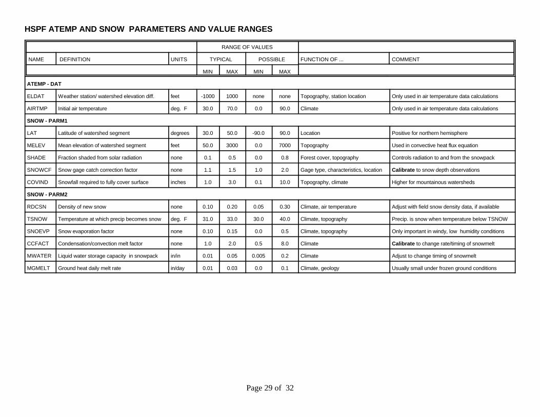
HSPF ATEMP AND SNOW PARAMETERS AND VALUE RANGES

RANGE OF VALUES

NAME DEFINITION UNITS TYPICAL POSSIBLE FUNCTION OF ... COMMENT

MIN MAX MIN MAX

ATEMP - DAT

ELDAT Weather station/ watershed elevation diff. feet -1000 1000 none none Topography, station location Only used in air temperature data calculations

AIRTMP Initial air temperature deg. F 30.0 70.0 0.0 90.0 Climate Only used in air temperature data calculations

SNOW - PARM1

LAT Latitude of watershed segment degrees 30.0 50.0 -90.0 90.0 Location Positive for northern hemisphere

MELEV Mean elevation of watershed segment feet 50.0 3000 0.0 7000 Topography Used in convective heat flux equation

SHADE Fraction shaded from solar radiation none 0.1 0.5 0.0 0.8 Forest cover, topography Controls radiation to and from the snowpack

SNOWCF Snow gage catch correction factor none 1.1 1.5 1.0 2.0 Gage type, characteristics, location Calibrate to snow depth observations

COVIND Snowfall required to fully cover surface inches 1.0 3.0 0.1 10.0 Topography, climate Higher for mountainous watersheds

SNOW - PARM2

RDCSN Density of new snow none 0.10 0.20 0.05 0.30 Climate, air temperature Adjust with field snow density data, if available

TSNOW Temperature at which precip becomes snow deg. F 31.0 33.0 30.0 40.0 Climate, topography Precip. is snow when temperature below TSNOW

SNOEVP Snow evaporation factor none 0.10 0.15 0.0 0.5 Climate, topography Only important in windy, low humidity conditions

CCFACT Condensation/convection melt factor none 1.0 2.0 0.5 8.0 Climate Calibrate to change rate/timing of snowmelt

MWATER Liquid water storage capacity in snowpack in/in 0.01 0.05 0.005 0.2 Climate Adjust to change timing of snowmelt

MGMELT Ground heat daily melt rate in/day 0.01 0.03 0.0 0.1 Climate, geology Usually small under frozen ground conditions

Page 30 of 32

HSPF HYDROLOGY PARAMETERS AND VALUE RANGESRANGE OF VALUES

NAME DEFINITION UNITS TYPICAL POSSIBLE FUNCTION OF ... COMMENT

MIN MAX MIN MAX

PWAT - PARM2

FOREST Fraction forest cover none 0.0 0.50 0.0 0.95 Forest cover Only impact when SNOW is active

LZSN Lower Zone Nominal Soil Moisture Storage inches 3.0 8.0 2.0 15.0 Soils, climate Calibration

INFILT Index to Infiltration Capacity in/hr 0.01 0.25 0.001 0.50 Soils, land use Calibration, divides surface and subsurface flow

LSUR Length of overland flow feet 200 500 100 700 Topography Estimate from high resolution topo maps or GIS

SLSUR Slope of overland flow plane ft/ft 0.01 0.15 0.001 0.30 Topography Estimate from high resolution topo maps or GIS

KVARY Variable groundwater recession 1/inches 0.0 3.0 0.0 5.0 Baseflow recession variation Used when recession rate varies with GW levels

AGWRC Base groundwater recession none 0.92 0.99 0.85 0.999 Baseflow recession Calibration

PWAT - PARM3

PETMAX Temp below which ET is reduced deg. F 35.0 45.0 32.0 48.0 Climate, vegetation Reduces ET near freezing, when SNOW is active

PETMIN Temp below which ET is set to zero deg. F 30.0 35.0 30.0 40.0 Climate, vegetation Reduces ET near freezing, when SNOW is active

INFEXP Exponent in infiltration equation none 2.0 2.0 1.0 3.0 Soils variability Usually default to 2.0

INFILD Ratio of max/mean infiltration capacities none 2.0 2.0 1.0 3.0 Soils variability Usually default to 2.0

DEEPFR Fraction of GW inflow to deep recharge none 0.0 0.20 0.0 0.50 Geology, GW recharge Accounts for subsurface losses

BASETP Fraction of remaining ET from baseflow none 0.0 0.05 0.0 0.20 Riparian vegetation Direct ET from riparian vegetation

AGWETP Fraction of remaining ET from active GW none 0.0 0.05 0.0 0.20 Marsh/wetlands extent Direct ET from shallow GW

PWAT - PARM4

CEPSC Interception storage capacity inches 0.03 0.20 0.01 0.40 Vegetation type/density, land use Monthly values usually used

UZSN Upper zone nominal soil moisture storage inches 0.10 1.0 0.05 2.0 Surface soil conditions, land use Accounts for near surface retention

NSUR Manning’s n (roughness) for overland flow none 0.15 0.35 0.05 0.50 Surface conditions, residue, etc. Monthly values often used for croplands

INTFW Interflow inflow parameter none 1.0 3.0 1.0 10.0 Soils, topography, land use Calibration, based on hydrograph separation

IRC Interflow recession parameter none 0.5 0.7 0.3 0.85 Soils, topography, land use Often start with a value of 0.7, and then adjust

LZETP Lower zone ET parameter none 0.2 0.7 0.1 0.9 Vegetation type/density, root depth Calibration

Page 31 of 32

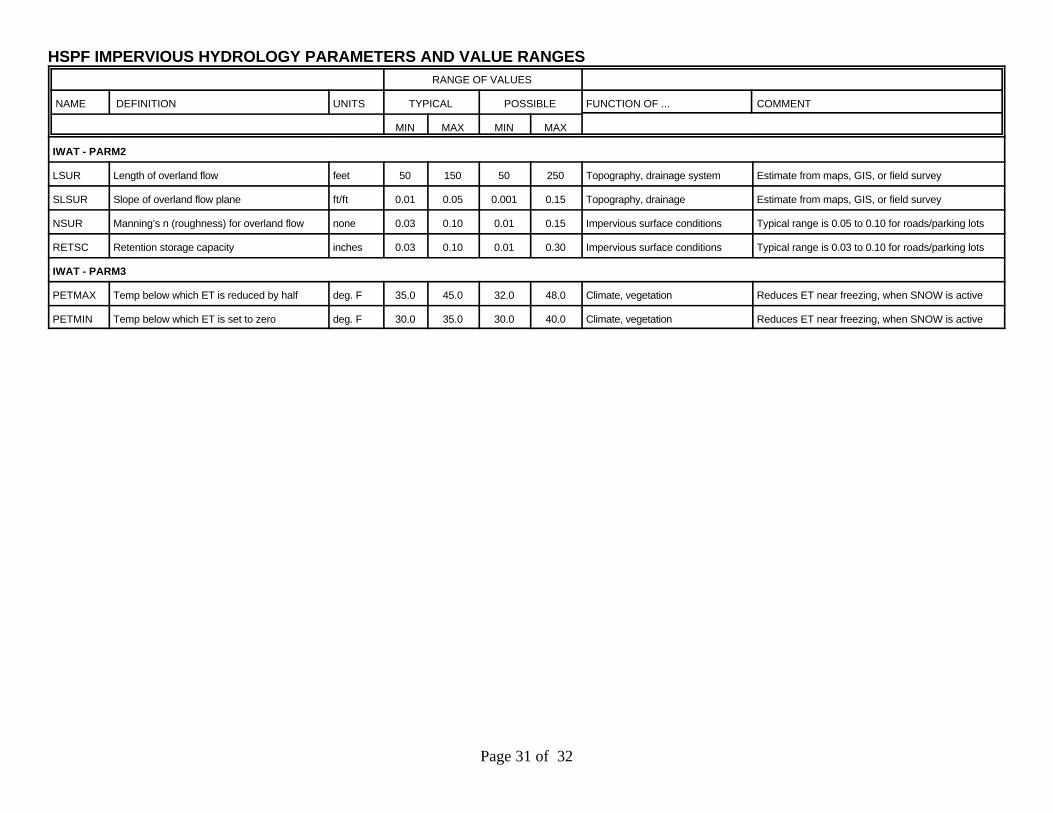
HSPF IMPERVIOUS HYDROLOGY PARAMETERS AND VALUE RANGESRANGE OF VALUES

NAME DEFINITION UNITS TYPICAL POSSIBLE FUNCTION OF ... COMMENT

MIN MAX MIN MAX

IWAT - PARM2

LSUR Length of overland flow feet 50 150 50 250 Topography, drainage system Estimate from maps, GIS, or field survey

SLSUR Slope of overland flow plane ft/ft 0.01 0.05 0.001 0.15 Topography, drainage Estimate from maps, GIS, or field survey

NSUR Manning’s n (roughness) for overland flow none 0.03 0.10 0.01 0.15 Impervious surface conditions Typical range is 0.05 to 0.10 for roads/parking lots

RETSC Retention storage capacity inches 0.03 0.10 0.01 0.30 Impervious surface conditions Typical range is 0.03 to 0.10 for roads/parking lots

IWAT - PARM3

PETMAX Temp below which ET is reduced by half deg. F 35.0 45.0 32.0 48.0 Climate, vegetation Reduces ET near freezing, when SNOW is active

PETMIN Temp below which ET is set to zero deg. F 30.0 35.0 30.0 40.0 Climate, vegetation Reduces ET near freezing, when SNOW is active

Page 32 of 32

HSPF HYDRAULIC PARAMETERS AND VALUE RANGESRANGE OF VALUES

NAME DEFINITION UNITS TYPICAL POSSIBLE FUNCTION OF ... COMMENT

MIN MAX MIN MAX

HYDR - PARM2

FTBDSN WDM data set number for FTABLE none none none 1 999 WDM File Used only if FTABLE is in WDM file

FTABNO FTABLE number in UCI file none none none 1 999 RCHRES block/ reach numbering Used only if FTABLE is in UCI file

LEN Stream reach (RCHRES) length miles 0.1 1.0 0.01 100 Topography, stream morphology Used only in computing auxiliary parameters

DELTH Stream reach length change in elevation feet 10 100 0.1 1000 Topography, stream morphology Used only for water quality and sediment

STCOR Stage correction factor feet 0.0 none 0.0 none Topography Dependent on elevation datum used

KS Routing weighting factor none 0.0 0.5 0.0 0.99 Channel slope, flow obstructions Use KS = 0.5

DB50 Bed sediment diameter inches 0.01 0.02 0.001 1.00 Channel bed properties Used only in sediment calculations

ADCALC - DATA

CRRAT Ratio of maximum to mean flow velocity none 1.5 2.0 1.0 3.5 Climate, vegetation Only used with water quality

VOL Initial stream channel water volume acre-feet 0.0 none 0.0 none Season, channel geometry, climate Initial volume in reach channel