The First XBT Science Workshop“ Building a Multi-Decadal Upper Ocean Temperature Record ” Building a Multi Decadal Upper Ocean Temperature Record

7-8 July, 2011, Melbourne, Australia

Basin Patterns of the upper ocean i f 1993 2008warming for 1993-2008

You-Soon Chang, Antony Rosati, Shaoqing Zhang, Gabriel Vecchi, Thomas Delworth and Andrew WittenbergThomas Delworth, and Andrew Wittenberg

Gophysical Fluid Dynamics Laboratory / NOAA

IntroductionLyman et al (2010 Nature) show a robust warming signal of the global upper ocean (0 700m)

L d J h (2008)

Lyman et al (2010, Nature) show a robust warming signal of the global upper ocean (0-700m).

They considered several sources of uncertainty associated with XBT correction and mappingmethod, which contributes to the differences among heat content estimations.

Lyman and Johnson (2008)

Levitus et al (2009)(2009)

Ishii and Kimono (2009)

Domingues et al (2008)

( )

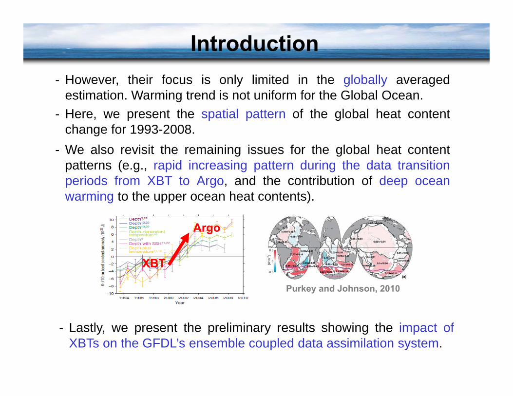
Introduction- However, their focus is only limited in the globally averaged

estimation. Warming trend is not uniform for the Global Ocean.- Here, we present the spatial pattern of the global heat content

change for 1993-2008.- We also revisit the remaining issues for the global heat content

patterns (e.g., rapid increasing pattern during the data transitionperiods from XBT to Argo, and the contribution of deep oceanwarming to the upper ocean heat contents).

XBT

Argo

L tl t th li i lt h i th i t f

Purkey and Johnson, 2010

- Lastly, we present the preliminary results showing the impact ofXBTs on the GFDL’s ensemble coupled data assimilation system.

Part 1: Data Analysis for HC700

Data:

- Levitus09 (gridded (1 x 1 x yearly) heat contents (Levitus et al., 2009))

- WOD09 (in situ T,S profiles (NODC World Ocean Database 2009))

- Monthly net heat flux at TOA from NCEP2

EN3 (gridded (1 x 1 x 42 levels X monthly) T S fields)- EN3 (gridded (1 x 1 x 42 levels X monthly) T, S fields)

Method:

- Global mean time series

- Spatial linear trend

EOF analysis with ENSO signal removed- EOF analysis with ENSO signal removed

Global mean time series and linear trend for HC700

Warming areas: Western Pacific, Atlantic, Indian Ocean…

Lyman et al., (2010)Cooling areas: Eastern Pacific, Gulf stream path…

Levitus09

Levitus09

Time series of HC700 show three characteristics as below:1. There are differences among the curves before 2000 (cooling, warming, no change).

Levitus09 used in this study shows warming trend during these periodLevitus09 used in this study shows warming trend during these period.2. All rapid increasing around 2000-2004.

3. All flatten out after around 2004.

Q1: HC700 is related to the no. obs (0-700m) ?Levitus09 HC700

We calculate the number of observations(WOD09) after binning into 3 x 3 x 0-700m x1 year.

Levitus09 HC700

y

WOD09 (raw)

There are high freq. datasets in 1998 and2001 around the coastal areas obtained byintensive CTD observation projects duringintensive CTD observation projects duringthese years. So, we remove the grid boxthat the total number is not within the 3sigma range.

WOD09 (filtered) WOD09 (XBT) WOD09 (PFL-Argo)

No significant change related to the HC700around 2000-2004 and after 2005.

( ) WOD09 (XBT) WOD09 (PFL-Argo)

Due to XBT and Argo array

Q1: HC700 is related to the no. obs (0-700m) ?

Levitus09 HC700 linear trend

WOD09 (raw) no. data linear trend WOD09 (filtered) no. data linear trend

There is no relationship of the spatial linear patterns.Most oceans show increasing pattern of the number of data due to Argo array since 2000.

Q1: HC700 is related to the no. obs (700m-2000m) ?Levitus09 HC700Levitus09 HC700

WOD09 (filtered)Due to Argo array

I i tt f l AIncreasing pattern from only Argo array.No relationship between two time series and spatial patterns.

Q1: HC700 is related to the no. obs (2000m-5000m) ?Levitus09 HC700Levitus09 HC700

WOD09 (filtered)

N i ifi t l ti hi b t t ti i d ti l ttNo significant relationship between two time series and spatial patterns.There are very sparse datasets below 2000 m for 1993-2008, so we can not confirm anyreliable trend.

Q2: HC700 is related to radiation flux of TOA ?

ΣQ=HCHC/dt = QHC/dt = QQ=0, flattening of HCQ>0, increasing of HCQ<0 d i f HC

NCEP2Q<0, decreasing of HC

>0Increasing

HCFlattening HCFlattening or

decreasing HC (?)

=0=0 or <0

We calculate net heat flux (low pass filtering after annual cycle removed) at TOA from NCEP2d t Th i li bl l ti hi b t t i ll ft 2000data. There is a reliable relationship between two curves especially after 2000, so we canconclude that the rapid increasing pattern is not a spurious due to any data sampling issue,but a real signal that is dynamically related to the radiation flux of TOA.

Q3: How is the spatial pattern of the heat content ?

Warming areas: Western Pacific, Atlantic, Indian Ocean…

Cooling areas: Eastern Pacific, Gulf stream path…

Levitus09Levitus09

The spatial pattern seems to be strongly related to the ENSO patterns.

So we have investigated the regional variability in HC700 by using EOF analysis.

EOF pattern of the HC700

EOF patterns of HC700are strongly related to theg yENSO patterns.

So we attempt to removeSo, we attempt to removeENSO signal from thegridded HC data.

We use traditional simplemethods employing thelinear regression into thelinear regression into thedominant EOF time serieswith Nino indices (Kellyand Jones, 1996)

Black line: time series of each EOFs.Red line: regression using Nino indices with time lag

EOF series correlated with ENSO indices

Black line: time series of each EOFs.Red line: regression of selected Nino indices with time lag

We pick up 8 EOF series whose maximum correlation coefficients with

Red line: regression of selected Nino indices with time lag

p pselected Nino indices are more than 95% significant level.

Summary of the removal process

1 C l l t EOF f HC700 d t t i1. Calculate EOFs from HC700 raw data matrix.(EOF1(t)/w1(x,y), EOF2(t)/w2(x,y),…, EOF10(t)/w10(x,y))

2. Determine which EOFs are associated with the ENSO phenomenon byp ycalculating the cross correlation coefficient (>95% sig. Level) betweenEOFs and five ENSO indices (SOI, Nino3, Nino4, Nino3.4, andNino1+2)

3. Calculate the derived regression equationENSO1(t) = -0.5464*SOI(t)+0.0009ENSO2(t) = -0.2310*NINO4(t)-0.0016,……,ENSO8(t) = -0.2834*NINO3(t+7)+0.0102

4 Subtract the ENSO signal identified in the time series associated with4. Subtract the ENSO signal identified in the time series associated withEOFs.

CHC (Corrected Heat Content) (x,y,t) =HC (x,y,t) - ENSO1(t)w1(x,y) - ENSO2(t)w2(x,y) - ENSO3(t)w3(x,y) –HC (x,y,t) ENSO1(t)w1(x,y) ENSO2(t)w2(x,y) ENSO3(t)w3(x,y) ENSO4(t)w4(x,y) - ENSO5(t)w6(x,y) - ENSO6(t)w7(x,y) -ENSO7(t)w8(x,y) - ENSO8(t)w9(x,y)

Reconstruct time series uncorrelated with ENSO

Black line: time series of raw data.Red line: time series of reconstructed data uncorrelated with ENSO signal.

Strong interannual cycle has been reduced around the equatorial area whereENSO signals are dominant.

Around off-equatorial areas, reconstruct time series keep the variability whichmay not be related with ENSO phenomena.

EOF patterns uncorrelated with ENSO

Levitus09 (raw)

Warming pattern

ENSO pattern

EOF 1st mode shows a stead warming trend. This warming pattern is shown in the AtlanticOcean especially including subpolar gyre and Indian Ocean, which is very similar with thep y g p gy ylinear trend pattern of HC700 raw data.

In the 2nd mode, ENSO pattern around the Pacific Ocean still remained. There are possiblelimitations with the ENSO-removal method used in this study, which employs the linearregression on the time series of some ENSO index (ENSO-unrelated variations can occur inregression on the time series of some ENSO index (ENSO unrelated variations can occur inthe ENSO index. ENSO-related variations occur in step around the globe. Observed ENSOevolution does not involve in just a couple of EOF patterns. ENSO has nonlinearcharacteristic…..) .

Q4: How is the deep ocean ?

Indian Ocean Pacific Ocean Atlantic Ocean

B i EN3 d t i ti t l t t t d f 1993 2009By using EN3 data, we investigate zonal mean temperature trend for 1993-2009 upto 5500 m depth.

In the Indian and Atlantic Ocean, we confirm significant warming trend below 1000m and around the deep abyssal ocean which may related to the upper oceanm and around the deep abyssal ocean, which may related to the upper oceanwarming around these basins (Purkey and Johnson, 2010; Song and Colberg2011).

Conclusion

Q1: HC700 is related to the different sampling era ?The rapid increasing pattern of HC700 around 2000-2004 is not related to thenumber of data around the data transition periods from XBT to Argonumber of data around the data transition periods from XBT to Argo.

Q2: HC700 is related to the radiation change of TOA ?Rapid increasing pattern around 2000-2004 is associated with the radiation changep g p gof the top of atmosphere. They are dynamically related to each other and weconfirmed it by using observation (reanalysis).

Q3: How is the spatial pattern of the heat content for 1993 2008?Q3: How is the spatial pattern of the heat content for 1993-2008?Western Pacific, Atlantic, and Indian Oceans show significant warming trend duringthis period. When we remove ENSO signals, we obtain more stead warming trendas the 1st EOF mode around the Atlantic and Indian Ocean.

Q4: How is the deep ocean ?Deep ocean warming trend is found especially around the abyssal oceans ofAtlantic and Indian Ocean which may be related to the upper ocean warmingAtlantic and Indian Ocean, which may be related to the upper ocean warming.

Part 2: GFDL ECDA (Ensemble Coupled Data Assimilation System)

Model:

Part 2: GFDL ECDA (Ensemble Coupled Data Assimilation System)

- Base model: GFDL CM2.1

- Assimilation scheme: Ensemble Kalman Filtering with cov(T,S)

Initialization for 380 yrs from the 1860 fixed year radiative forcing run- Initialization for 380 yrs from the 1860 fixed year radiative forcing run

- IPCC historical run with time varying GHGNA since 1861.

- Observed ocean profiles since 1976 with :

WOD09 (XBT, MBT, CTD, MRB, OSD)

Argo (2000-present)

GTSPP (2009-present)GTSPP (2009 present)

Experiment:

- ECDA_full (1993-2006) (MBT, CTD, MRB, OSD, XBT, and Argo)

- ECDA_no_XBT (1993-2006) (MBT, CTD, MRB, OSD, and Argo)

GFDL ECDA

Cartoon of how (a) data assimilation (red arrow) in the GFDL coupled modeltransfers observational information into the coupled component by exchangefl (bl k ) d (b) bl filt d t th b bilitfluxes (black arrows), and (b) an ensemble filter updates the probabilitydistribution. [Zhang et al., 2007, 2010]

Oceanic data management system for ECDA

Step 1: Data Mirroring System( WOD09, Argo, GTSPP )

[QC P Ch t l

Step 2: Quality Control System(Real Time + Delayed Mode )

[QC Process, Chang et al., (2009)]

[DMQC result]

Step 3: Ensemble Coupled DataAssimilation SystemAssimilation System

HC700 difference between ECDA_no_xbt and ECDA_full

1996

2006

The XBT effect can be found globally especially along the ocean gyre systems.

There are also significant difference in the Southern OceanThere are also significant difference in the Southern Ocean

The difference is getting reduced in time.

RMSE change between ECDA_no_xbt and ECDA_full

RMSE for HC (0-700m) RMSE for HC (0-50m)

RMSE for HC (50-300m) RMSE for HC (600-2000m)

There are a little bit different patterns for RMSE change in depth.

Surface layer: XBT effects most rapidly decrease.

Subsurface layer below 600 m: XBT effect remains even after Argo periods.

Subsurface T,S change between ECDA_no_xbt and ECDA_full

XBT affects the assimilated salinity field as wellfield as well.

T/S difference reduced in time at 15 and 205m.

At 618m, the difference remains even after Argo period.

HC700 from observations and ECDA experiments

ECDA_no_xbt shows significant bias both for Atlantic and Indian Ocean.

ECDA_full shows bias in the Pacific, but variability is reasonable.reasonable.

EN3 shows cold bias for Atlantic and Pacific during Argo periods.and Pacific during Argo periods.

XBT plays an important role for the HC simulation.the HC simulation.

Conclusion

Q: How is the impact of XBTs on the GFDL’s ensemblecoupled data assimilation system.coupled data assimilation system.

We showed the XBT effects on the ECDA systemWe showed the XBT effects on the ECDA system

1. even in the Southern Oceans.

2. even after Argo periods especially for the subsurface depths.

3. even for salinity and other fields.

4. especially for the HC700 reanalysis around the Atlantic and Indian Oceans.

http://www.gfdl.noaa.gov/ocean-data-assimilation

Thank you !!a you감사합니다 !!

Quality Control

Quality Control [DMQC]

RTQC by DAC DMQC by DAC DMQC by this studyObjective estimation

• Our calibrations are in line with climatology and DAC results.• Many floats with salinity drift have not completed DMQC by DACs.

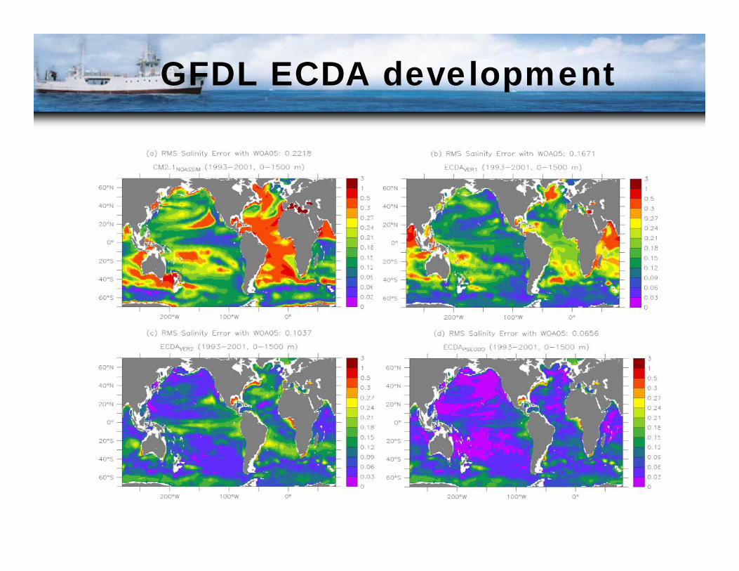
GFDL ECDA development