Roberto Basile Second University of Naples

Firm Heterogeneity and Regional Business Cycles Differentials

Conferenza ISTAT, Roma, 21 Novembre 2011

Carmine PappalardoNational Institute of Statistics

Sergio de NardisNomisma

Background

Previous studies on regional business cycles (RBC):regional differences in the industrial mix are major responsible for RBC divergence

(Domazlicky, 1980; Carlino and DeFina, 1998)

But after controlling for industrial composition effects, these studies still find significant RBC heterogeneity

See also recent studies in Italy (Mastromarco and Woitek, 2007; Brasili and Brasili, 2009)

We claim that all previous studies, focusing on macroeconomic data, disregard the effect of firm heterogeneity in business cycle behaviour and thus they do not offer exhaustive explanations for RBC differences

Aim of the paper

In this paper we use microeconomic information and build a micro-econometric model so as to assess whether Northern and Southern firms in Italy show significant differences in cyclical behaviour, after having controlled for sector- and firm-specific factors that alter the transmission mechanism of exogenous shocks

Firm level business survey data

Monthly firm data on business cycle behaviour (ISTAT):Period: from April 2003 to December 2010The number of firms varies each periodTotal number of observations: 308,042

Dependent variable (yit): ordered indicator of firm production level:

y= 1 if the firm considers the current production level as lowy= 2 if the firm considers the current production level as normaly= 3 if the firm considers the current production level as high

Modelling firms’ business cycle behaviour

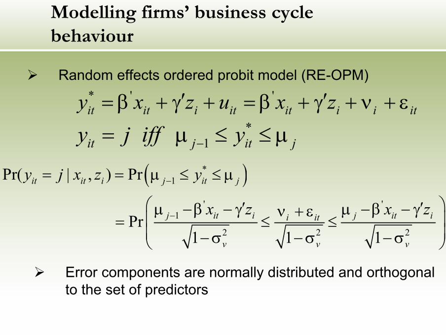
Random effects ordered probit model (RE-OPM)

Error components are normally distributed and orthogonal to the set of predictors

* ' 'it it i it it i i ity x z u x z′ ′= β + γ + = β + γ + ν + ε

*1it j it jy j iff y−= µ ≤ ≤ µ

( )*1

' '1

2 2 2

Pr( | , ) Pr

Pr1 1 1

it it i j it j

j it i j it ii it

v v v

y j x z y

x z x z

−

−

= = µ ≤ ≤ µ

′ ′µ −β − γ µ −β − γν + ε = ≤ ≤ −σ −σ −σ

FIRST STEP: Capturing national business cycle

We start by estimating a RE-OPM introducing only quarterly dummies (qt) as explanatory variables

The marginal effect of qt highly correlated with the cyclical component of the quarterly index of Italian industrial production => the production level is a good proxy of the deviance business cycle

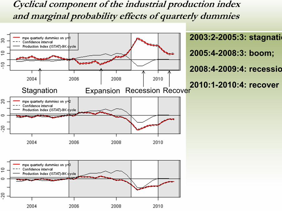
Cyclical component of the industrial production index and marginal probability effects of quarterly dummies

Stagnation Expansion Recession Recover

2003:2-2005:3: stagnation

2005:4-2008:3: boom;

2008:4-2009:4: recession

2010:1-2010:4: recover

SECOND STEP:Measuring the Southern effect

• We then include in the RE-OPM the interactions term South x qt in order to capture the average deviation of Southern firms’ business cycle from the Northern profile

• Results document sizable asymmetries in Northern and Southern firms business cycles positively related to the intensity of the national cycle: • Southern firms are more likely to reduce production levels in

periods of business cycle expansion and viceversa

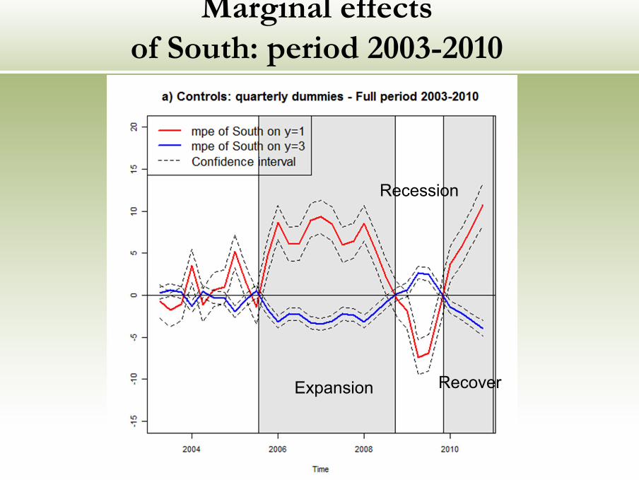
Marginal effectsof South: period 2003-2010

Recession

Expansion Recover

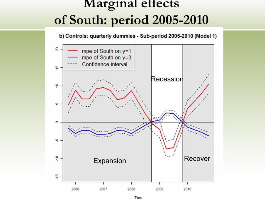
Marginal effectsof South: period 2005-2010

Recession

RecoverExpansion

THIRD STEP:Assessing the role of industry mix

We then include sectoral dummies (2-digit NACE Rev. 1 classification) in our model …

… but sectoral mix does not capture regional differences

Some evidence in favor of the hypothesis that industry composition has partially protected the South against the negative shocks of the world crisis (but no statistical significance)

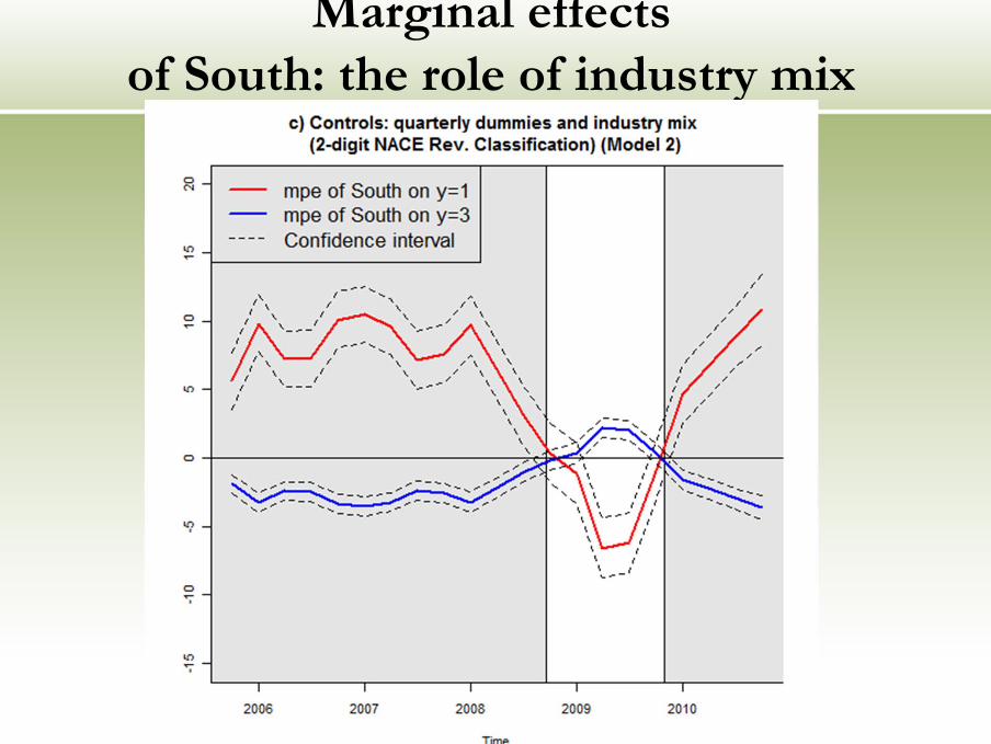
Marginal effectsof South: the role of industry mix

LAST STEP: Assessing the role of firm heterogeneity

Working hypothesis: various strand of literature suggest a strong firm heterogeneity along the business cycle, due to firm specific factors which alter the transmission mechanisms of exogenous shocks

Borrowing constraints (Firm size): Bernanke and Gertler (1995); Carlino and DeFina (1998); Dedola and Lippi (2000)

Liquidity constraints: Kiyotaki and Moore (2008)

Export propensity

Idiosyncratic demand shocks: Foster et al. (2008)

Capacity utilization: Fagnart et al. (1997); Fagnart et al. (1999)

If there is firm heterogeneity in business cycle behavior due to the factors mentioned above …

… regional differences in entrepreneurial composition (in terms of firm size and export propensity) and in firm behavior (in terms of demand conditions, liquidity conditions, capacity utilization and expectations) may help explain RBC differentials

LAST STEP: Assessing the role of firm heterogeneity

Finally, we test the role of local externalities:

The individual decision to raise or to reduce the production level is influenced by the production decision of nearby firms

LAST STEP: Assessing the role of firm heterogeneity

Microeconomic information from business cycle survey in Italy

Variables capturing firms’ heterogeneity in industrial business cycle behaviour

Log of firm size (number of employees) and its square term

Firm export propensity: export/total revenue

Firm specific demand conditions and expectations

Firm’s liquidity conditions and expectations

Firm’s capacity utilization

Local externalities: Employment density in the province where firm i is located X balance of production levels in the same province

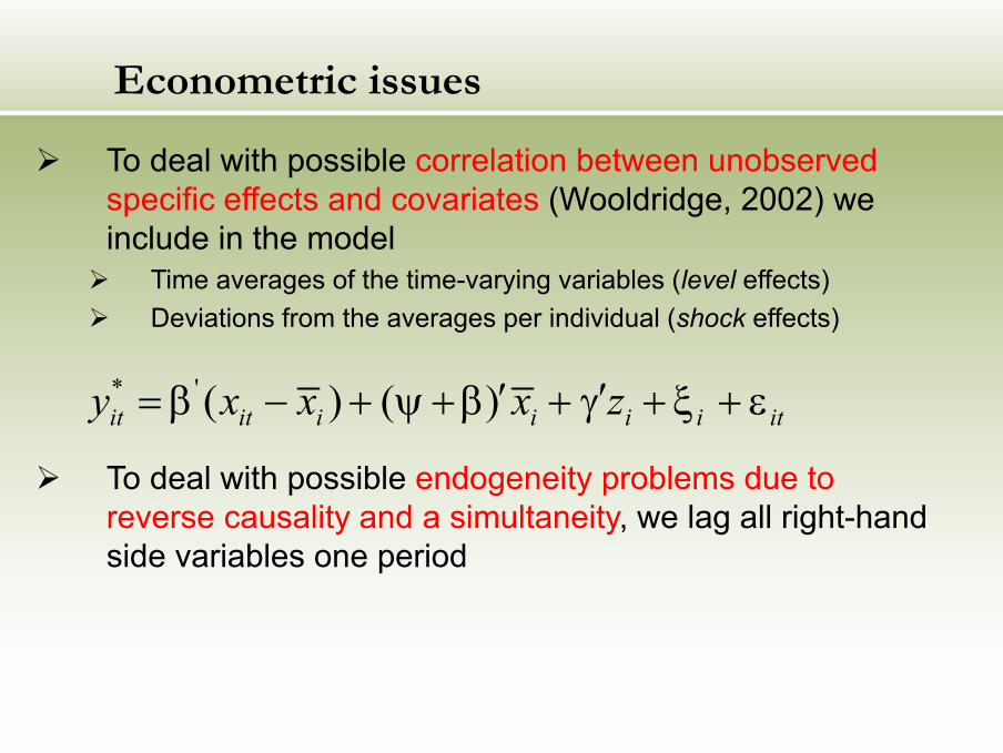
Econometric issues

To deal with possible correlation between unobserved specific effects and covariates (Wooldridge, 2002) we include in the model

Time averages of the time-varying variables (level effects)Deviations from the averages per individual (shock effects)

* ' ( ) ( )it it i i i i ity x x x z′ ′= β − + ψ +β + γ + ξ + ε

To deal with possible endogeneity problems due to reverse causality and a simultaneity, we lag all right-hand side variables one period

Estimation results

We have estimated six nested models introducing progressively firm size, export intensity, liquidity conditions, demand conditions, capacity utilizationand local externalitiesResults show that the full specification encompasses all the othersHowever, the most consistent improvements in the goodness of fit are observable with

firm sizeliquidity conditions demand conditions

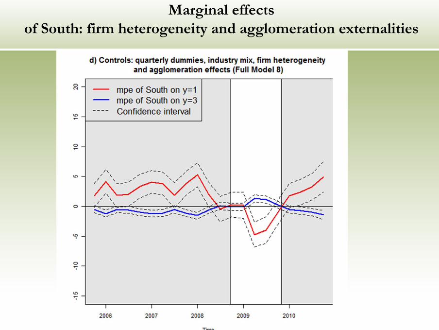
Marginal effectsof South: firm heterogeneity and agglomeration externalities

Marginal effectsof South: the role of industry mix

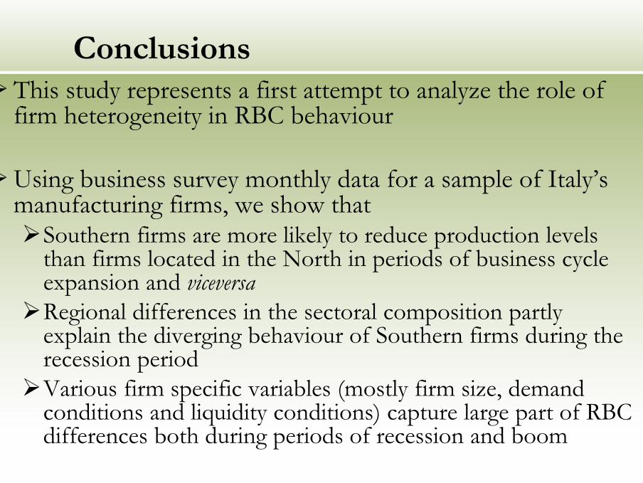
ConclusionsThis study represents a first attempt to analyze the role of firm heterogeneity in RBC behaviour

Using business survey monthly data for a sample of Italy’s manufacturing firms, we show that

Southern firms are more likely to reduce production levels than firms located in the North in periods of business cycle expansion and viceversaRegional differences in the sectoral composition partly explain the diverging behaviour of Southern firms during the recession periodVarious firm specific variables (mostly firm size, demand conditions and liquidity conditions) capture large part of RBC differences both during periods of recession and boom

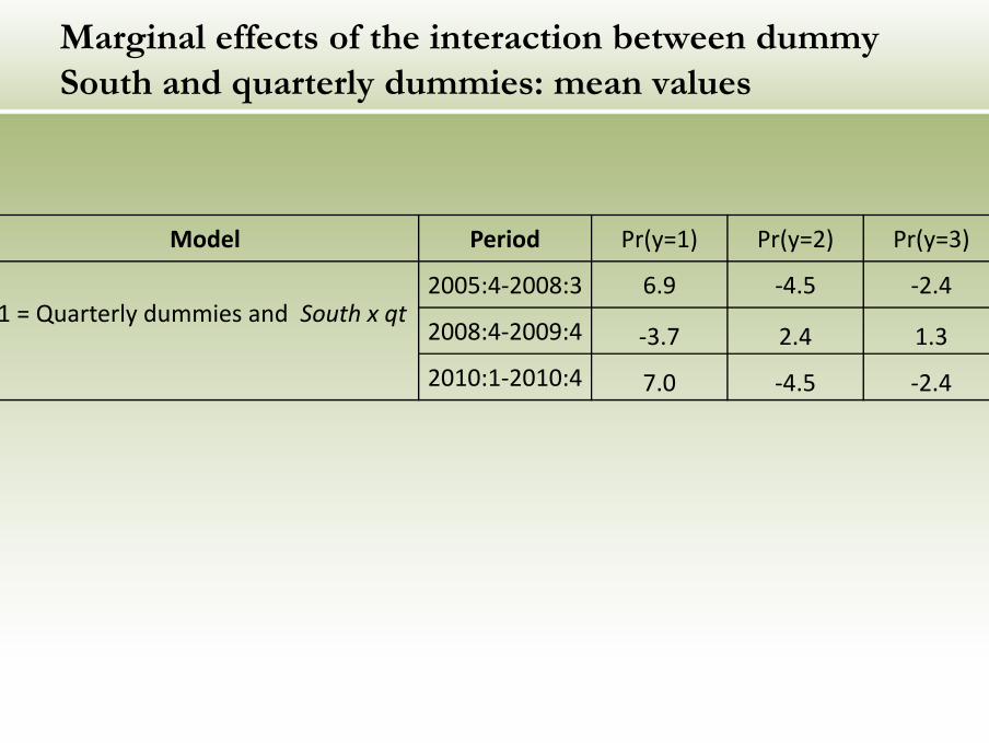
Marginal effects of the interaction between dummy South and quarterly dummies: mean values

Model Period Pr(y=1) Pr(y=2) Pr(y=3)

1 = Quarterly dummies and South x qt2005:4-2008:3 6.9 -4.5 -2.4

2008:4-2009:4 -3.7 2.4 1.32010:1-2010:4 7.0 -4.5 -2.4

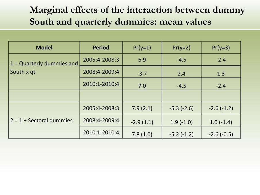
Marginal effects of the interaction between dummy South and quarterly dummies: mean values

Model Period Pr(y=1) Pr(y=2) Pr(y=3)

1 = Quarterly dummies and South x qt

2005:4-2008:3 6.9 -4.5 -2.4

2008:4-2009:4 -3.7 2.4 1.3

2010:1-2010:4 7.0 -4.5 -2.4

2 = 1 + Sectoral dummies

2005:4-2008:3 7.9 (2.1) -5.3 (-2.6) -2.6 (-1.2)

2008:4-2009:4 -2.9 (1.1) 1.9 (-1.0) 1.0 (-1.4)

2010:1-2010:4 7.8 (1.0) -5.2 (-1.2) -2.6 (-0.5)

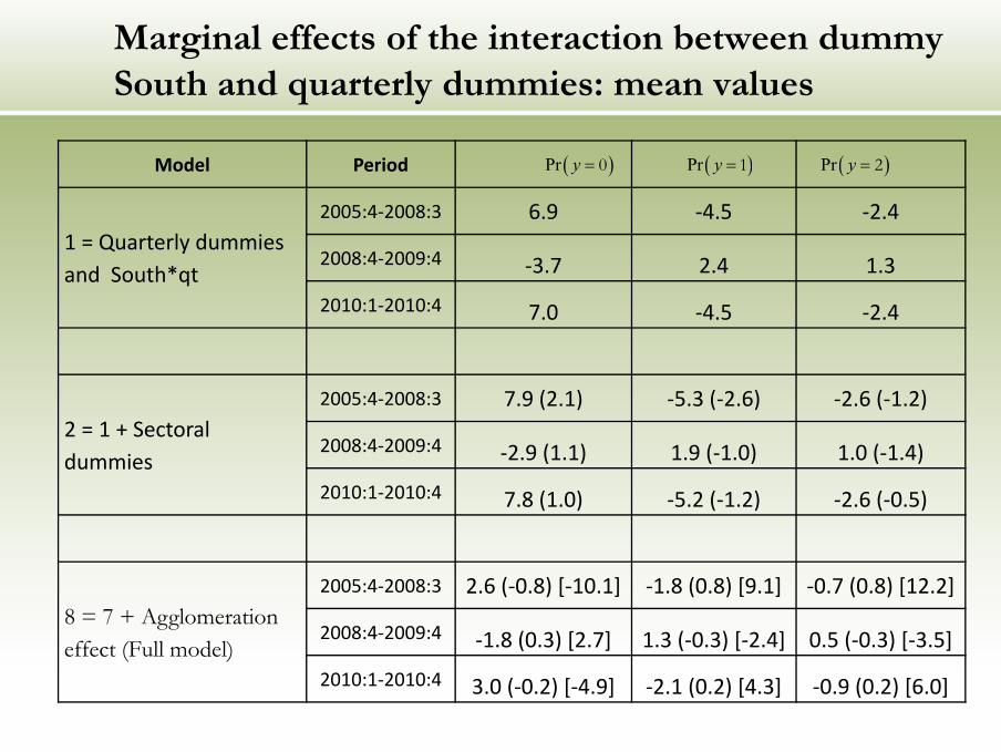
Marginal effects of the interaction between dummy South and quarterly dummies: mean values

( )Pr y = 0 ( )Pr y = 1 ( )Pr y = 2Model Period

1 = Quarterly dummies and South*qt

2005:4-2008:3 6.9 -4.5 -2.4

2008:4-2009:4 -3.7 2.4 1.3

2010:1-2010:4 7.0 -4.5 -2.4

2 = 1 + Sectoraldummies

2005:4-2008:3 7.9 (2.1) -5.3 (-2.6) -2.6 (-1.2)

2008:4-2009:4 -2.9 (1.1) 1.9 (-1.0) 1.0 (-1.4)

2010:1-2010:4 7.8 (1.0) -5.2 (-1.2) -2.6 (-0.5)

8 = 7 + Agglomeration effect (Full model)

2005:4-2008:3 2.6 (-0.8) [-10.1] -1.8 (0.8) [9.1] -0.7 (0.8) [12.2]

2008:4-2009:4 -1.8 (0.3) [2.7] 1.3 (-0.3) [-2.4] 0.5 (-0.3) [-3.5]

2010:1-2010:4 3.0 (-0.2) [-4.9] -2.1 (0.2) [4.3] -0.9 (0.2) [6.0]

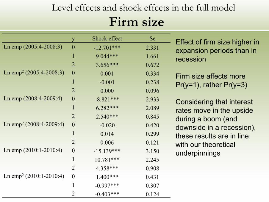
Level effects and shock effects in the full modelFirm size

y Shock effect SeLn emp (2005:4-2008:3) 0 -12.701*** 2.331

1 9.044*** 1.6612 3.656*** 0.672

Ln emp2 (2005:4-2008:3) 0 0.001 0.3341 -0.001 0.2382 0.000 0.096

Ln emp (2008:4-2009:4) 0 -8.821*** 2.9331 6.282*** 2.0892 2.540*** 0.845

Ln emp2 (2008:4-2009:4) 0 -0.020 0.4201 0.014 0.2992 0.006 0.121

Ln emp (2010:1-2010:4) 0 -15.139*** 3.1501 10.781*** 2.2452 4.358*** 0.908

Ln emp2 (2010:1-2010:4) 0 1.400*** 0.4311 -0.997*** 0.3072 -0.403*** 0.124

Effect of firm size higher in expansion periods than in recession

Firm size affects more Pr(y=1), rather Pr(y=3)

Considering that interest rates move in the upside during a boom (and downside in a recession), these results are in line with our theoretical underpinnings

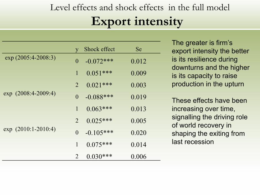
Level effects and shock effects in the full modelExport intensity

y Shock effect Seexp (2005:4-2008:3) 0 -0.072*** 0.012

1 0.051*** 0.009

2 0.021*** 0.003exp (2008:4-2009:4) 0 -0.088*** 0.019

1 0.063*** 0.013

2 0.025*** 0.005exp (2010:1-2010:4) 0 -0.105*** 0.020

1 0.075*** 0.014

2 0.030*** 0.006

The greater is firm’s export intensity the better is its resilience during downturns and the higher is its capacity to raise production in the upturn

These effects have been increasing over time, signalling the driving role of world recovery in shaping the exiting from last recession

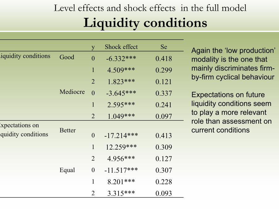
Level effects and shock effects in the full modelLiquidity conditions

y Shock effect SeLiquidity conditions Good 0 -6.332*** 0.418

1 4.509*** 0.2992 1.823*** 0.121

Mediocre 0 -3.645*** 0.3371 2.595*** 0.2412 1.049*** 0.097

Expectations on liquidity conditions Better

0 -17.214*** 0.4131 12.259*** 0.3092 4.956*** 0.127

Equal 0 -11.517*** 0.3071 8.201*** 0.2282 3.315*** 0.093

Again the ‘low production’ modality is the one that mainly discriminates firm-by-firm cyclical behaviour

Expectations on future liquidity conditions seem to play a more relevant role than assessment on current conditions

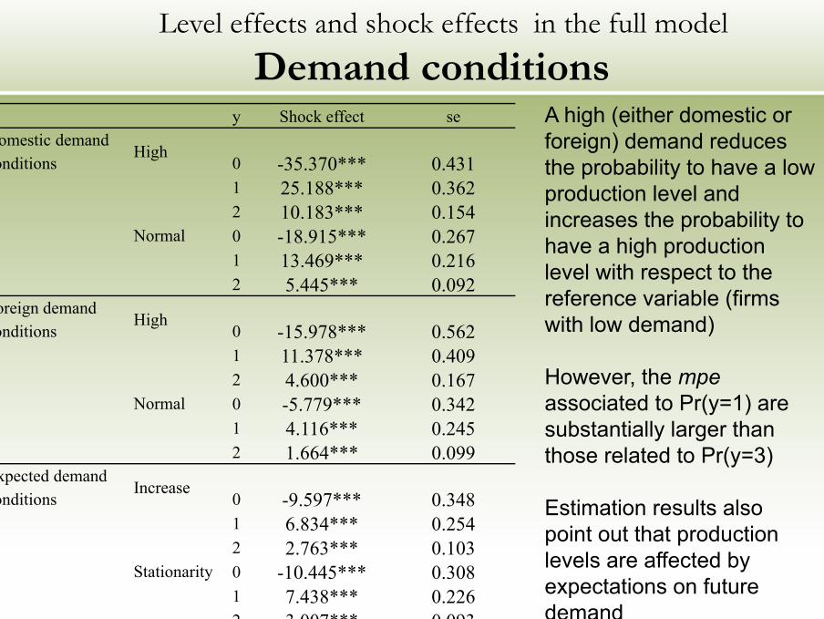
Level effects and shock effects in the full modelDemand conditions

y Shock effect seDomestic demandconditions

High0 -35.370*** 0.4311 25.188*** 0.3622 10.183*** 0.154

Normal 0 -18.915*** 0.2671 13.469*** 0.2162 5.445*** 0.092

Foreign demandconditions

High0 -15.978*** 0.5621 11.378*** 0.4092 4.600*** 0.167

Normal 0 -5.779*** 0.3421 4.116*** 0.2452 1.664*** 0.099

Expected demand conditions

Increase0 -9.597*** 0.3481 6.834*** 0.2542 2.763*** 0.103

Stationarity 0 -10.445*** 0.3081 7.438*** 0.2262 3.007*** 0.093

A high (either domestic or foreign) demand reduces the probability to have a low production level and increases the probability to have a high production level with respect to the reference variable (firms with low demand)

However, the mpeassociated to Pr(y=1) are substantially larger than those related to Pr(y=3)

Estimation results also point out that production levels are affected by expectations on future demand

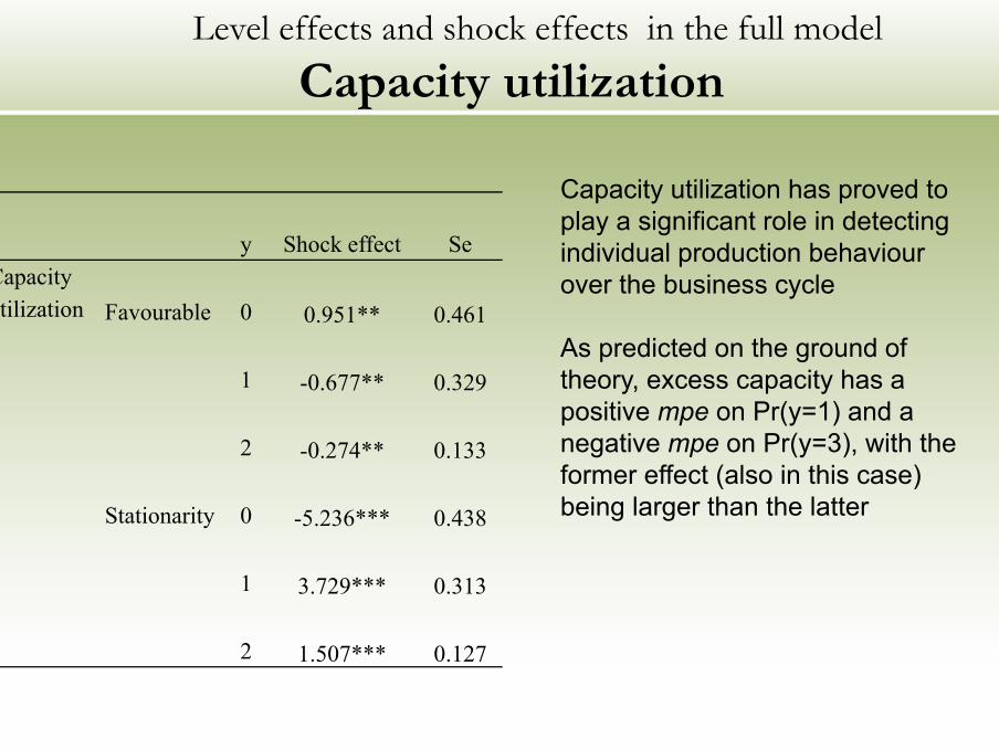
Level effects and shock effects in the full modelCapacity utilization

y Shock effect SeCapacity utilization Favourable 0 0.951** 0.461

1 -0.677** 0.329

2 -0.274** 0.133

Stationarity 0 -5.236*** 0.438

1 3.729*** 0.313

2 1.507*** 0.127

Capacity utilization has proved to play a significant role in detecting individual production behaviour over the business cycle

As predicted on the ground of theory, excess capacity has a positive mpe on Pr(y=1) and a negative mpe on Pr(y=3), with the former effect (also in this case) being larger than the latter

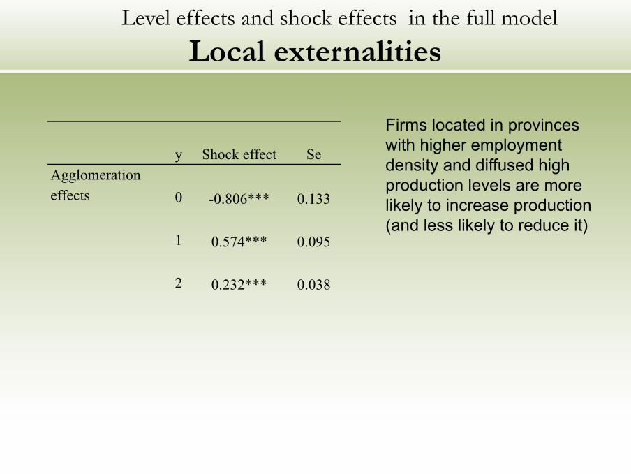
Level effects and shock effects in the full modelLocal externalities

y Shock effect SeAgglomeration effects 0 -0.806*** 0.133

1 0.574*** 0.095

2 0.232*** 0.038

Firms located in provinces with higher employment density and diffused high production levels are more likely to increase production (and less likely to reduce it)