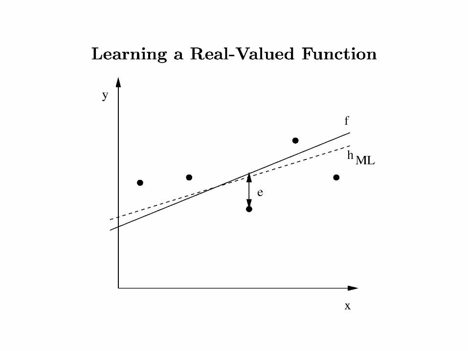
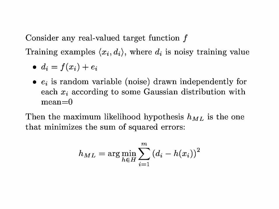
Basics of Statistical Estimation

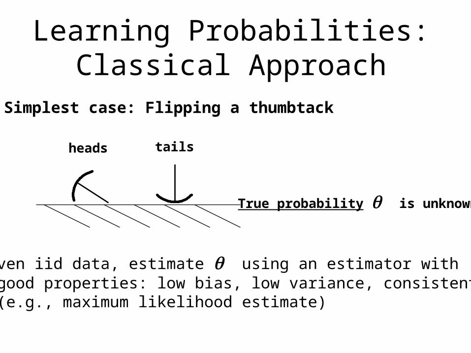
Learning Probabilities:Classical Approach

Simplest case: Flipping a thumbtack

tailsheads

True probability is unknown

Given iid data, estimate using an estimator with good properties: low bias, low variance, consistent (e.g., maximum likelihood estimate)

Maximum Likelihood Principle

Choose the parameters that maximizethe probability of the observed data

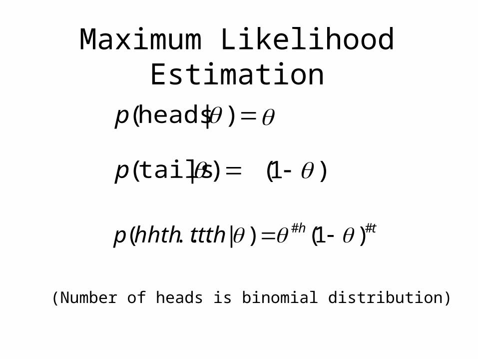
Maximum Likelihood Estimation

)|tails( p

)|heads( p

)1(

thttthhhthp ## )1()|...(

(Number of heads is binomial distribution)

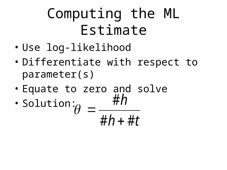
Computing the ML Estimate

• Use log-likelihood

• Differentiate with respect to parameter(s)

• Equate to zero and solve

• Solution:

th

h

##

#

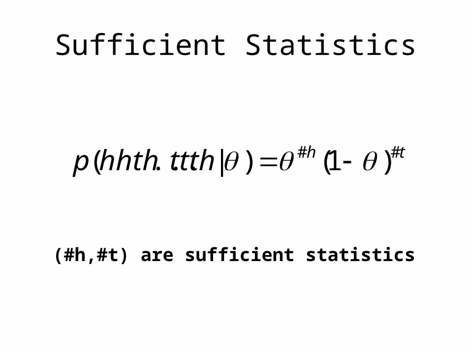
Sufficient Statistics

(#h,#t) are sufficient statistics

thttthhhthp ## )1()|...(

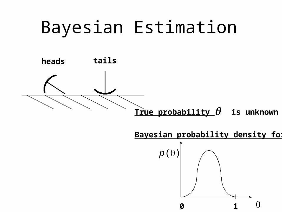
Bayesian Estimation

tailsheads

True probability is unknown

Bayesian probability density for

p()

0 1

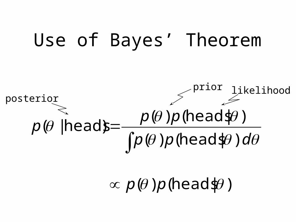
Use of Bayes’ Theorem

dpp

ppp

)|heads()(

)|heads()()heads|(

prior likelihoodposterior

)|heads()( pp

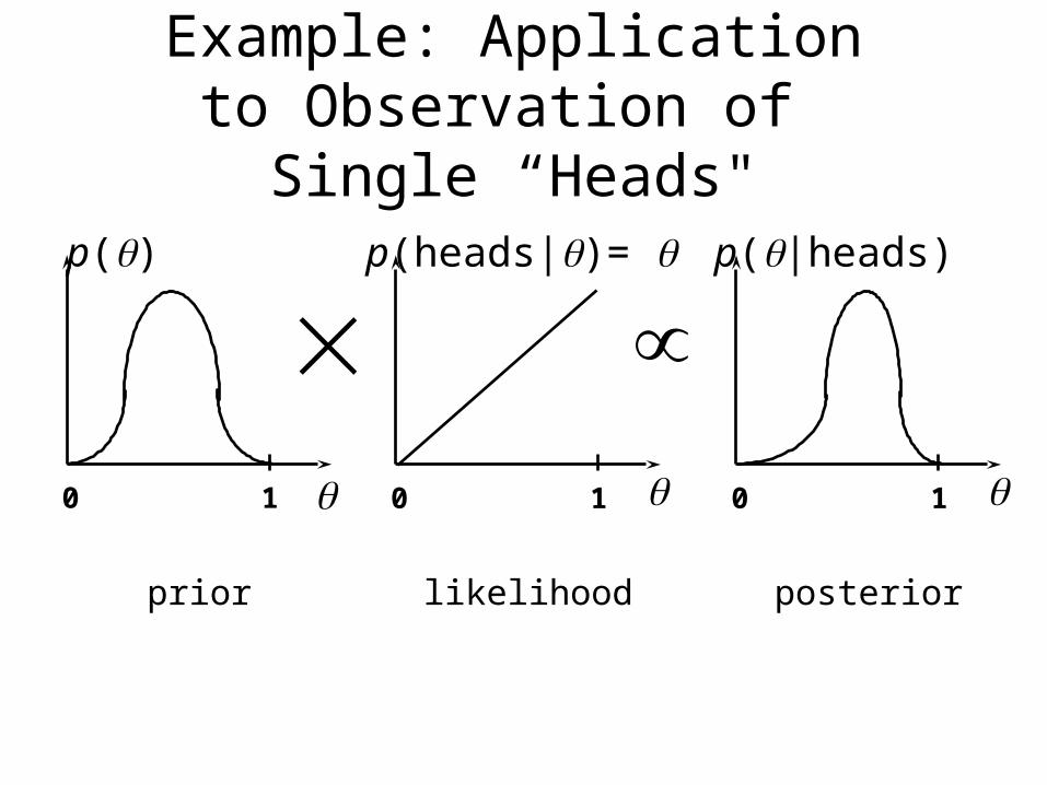
Example: Application to Observation of Single “Heads"

p(|heads)

0 1

p()

0 1

p(heads|)=

0 1

prior likelihood posterior

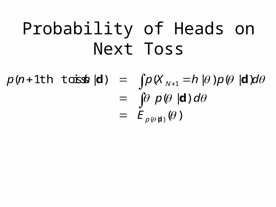
Probability of Heads on Next Toss

)(

)|(

)|()|()| is th toss1(

)|(

1

d

d

dd

p

N

E

dp

dphXphnp

MAP Estimation

• Approximation:– Instead of averaging over all parameter values– Consider only the most probable value

(i.e., value with highest posterior probability)

• Usually a very good approximation,and much simpler

• MAP value ≠ Expected value• MAP → ML for infinite data

(as long as prior ≠ 0 everywhere)

Prior Distributions for

• Direct assessment

• Parametric distributions

–Conjugate distributions(for convenience)

–Mixtures of conjugate distributions

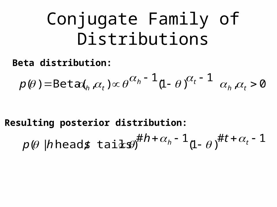
Conjugate Family of Distributions

0,1

)1(1

),Beta()( thth

thp

1#)1(

1# tails),heads |(

th ththp

Beta distribution:

Resulting posterior distribution:

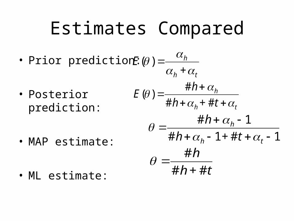
Estimates Compared

• Prior prediction:

• Posterior prediction:

• MAP estimate:

• ML estimate:

th

h

t+h

hE

# #

# )(

th

hE

+

)(

1 # +1#

1#

th

h

th

h

th

h

# +#

#

Intuition

• The hyperparameters h and t can be

thought of as imaginary counts from our prior

experience, starting from "pure ignorance"

• Equivalent sample size = h + t

• The larger the equivalent sample size, the

more confident we are about the true

probability

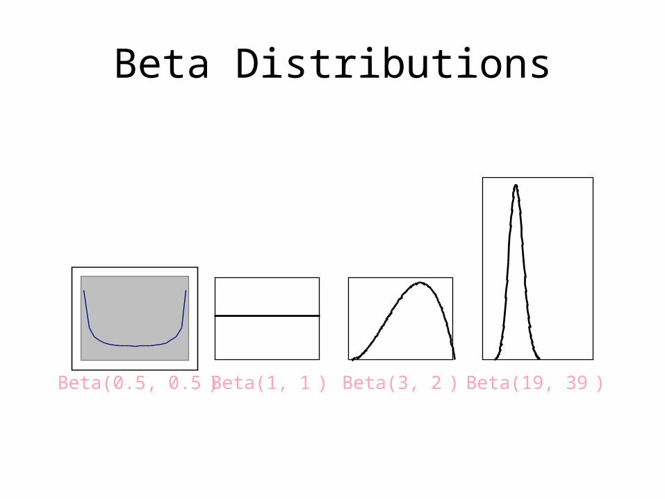
Beta Distributions

Beta(3, 2 )Beta(1, 1 ) Beta(19, 39 )Beta(0.5, 0.5 )

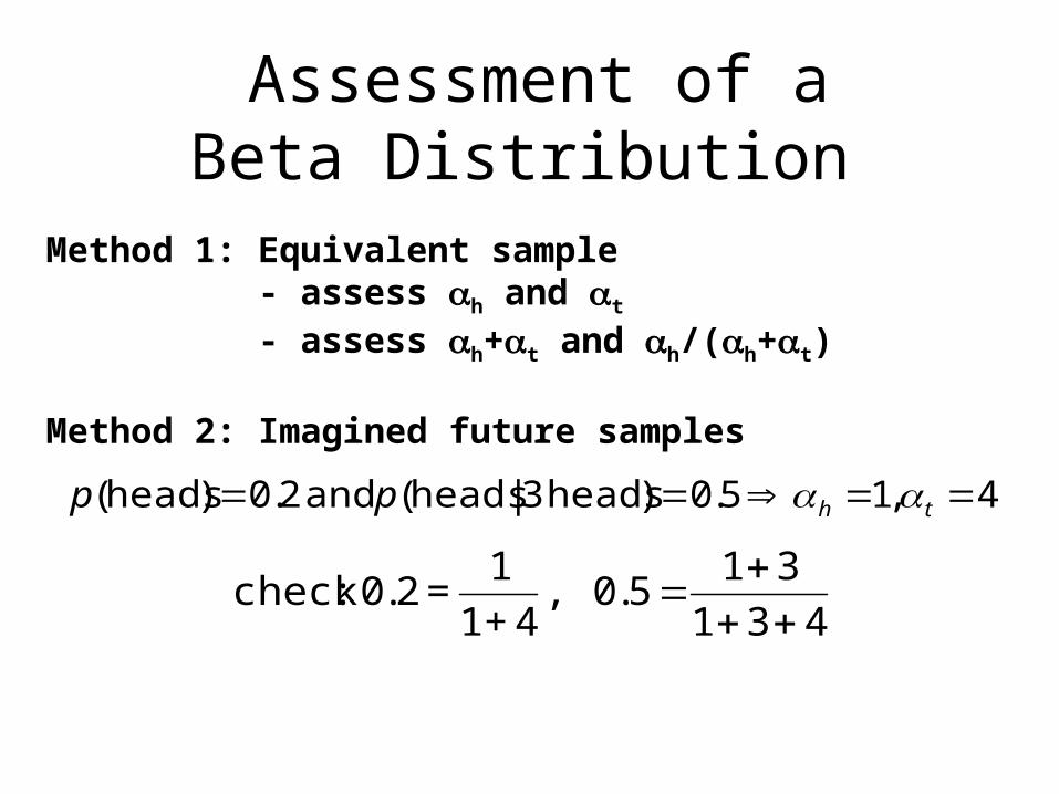
Assessment of aBeta Distribution

Method 1: Equivalent sample- assess h and t

- assess h+t and h/(h+t)

Method 2: Imagined future samples

4,15.0)heads 3|heads( and 2.0)heads( thpp

check: .2 =1

1+ 40 0 5

1 3

1 3 4, .

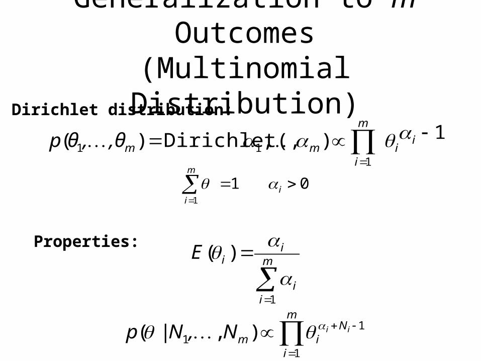
Generalization to m Outcomes(Multinomial Distribution)

1 ),,Dirichlet()(1

11

ii

m

imm,θ,θp

m

i

Nim

iiN,Np1

11 ),|(

Dirichlet distribution:

m

ii

iiE

1

)(

Properties:

011

i

m

i

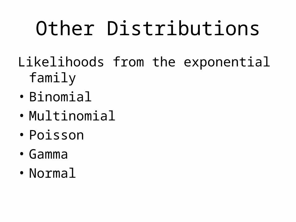
Other Distributions

Likelihoods from the exponential family

• Binomial

• Multinomial

• Poisson

• Gamma

• Normal