Embed Size (px)
Citation preview
Basics of radiation and antennas
P. Hazdra, M. Mazanek,….
Department of Electromagnetic Field
Czech Technical University in Prague, FEE
www.elmag.org
v. 16.2.2014
Literature
• C. A. Balanis, Antenna Theory and Design, Wiley, 2005
• T. A. Milligan, Modern Antenna Design, Wiley, 2005
• J. D. Kraus, Antennas, McGraw-Hill, 1997
• S. J. Orfanidis, EM Waves and antennas, online http://www.ece.rutgers.edu/~orfanidi/ewa/
• M. Mazánek, P. Pechač, J. Vokurka, Antény a šíření elektromagnetických vln, skripta ČVUT, Praha 2007
• IEEE XPLORE http://ieeexplore.ieee.org/ (full text papers of journals involving antennas)
2
Content • Radiation, what is an antenna?
• Antenna as a transformer of guided waves into free-space waves
• Circuit model of antenna
• Solution of radiation problems in terms of auxiliary vector potentials
• Elementary radiator – infinitesimaly small element of current (Hertz dipole)
• Fields and parameters of elementary dipole
• Radiation zones, directional properties (rad. pattern), polarization
• Overview of antenna types and their applications
3

Antenna is…
• Passive filter, both in frequency and spatial domain
• Component transforming guided waves to waves in free space (that is actually 3D spherical waveguide)
• Very important component of the whole communication channel
• „The best amplifier“
4
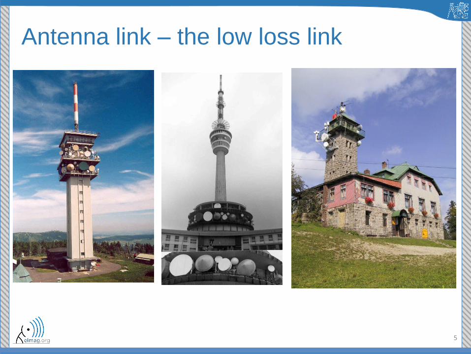
Antenna link – the low loss link
5
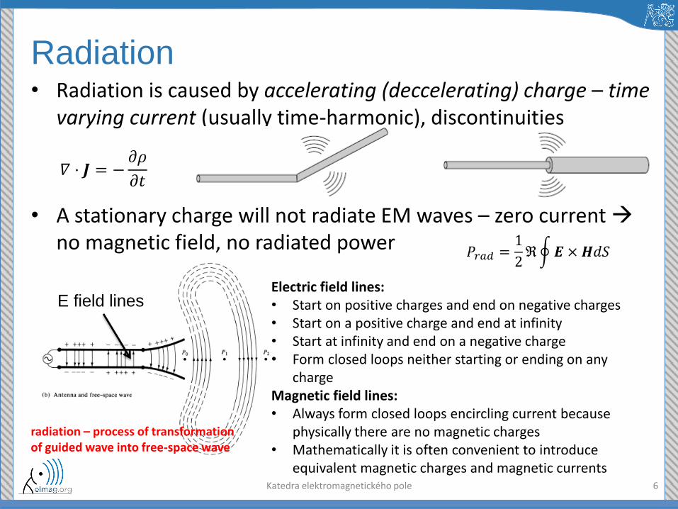
Radiation • Radiation is caused by accelerating (deccelerating) charge – time
varying current (usually time-harmonic), discontinuities
• A stationary charge will not radiate EM waves – zero current no magnetic field, no radiated power
Katedra elektromagnetického pole 6
𝛻 ⋅ 𝑱 = −𝜕𝜌
𝜕𝑡
𝑃𝑟𝑎𝑑 =1
2ℜ 𝑬 × 𝑯𝑑𝑆
E field lines Electric field lines: • Start on positive charges and end on negative charges • Start on a positive charge and end at infinity • Start at infinity and end on a negative charge • Form closed loops neither starting or ending on any
charge Magnetic field lines: • Always form closed loops encircling current because
physically there are no magnetic charges • Mathematically it is often convenient to introduce
equivalent magnetic charges and magnetic currents
radiation – process of transformation of guided wave into free-space wave
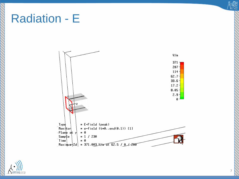
Radiation - E
7
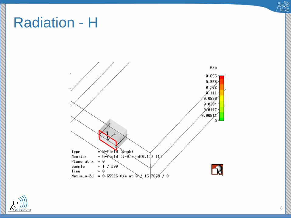
Radiation - H
8
Radiation - E
9
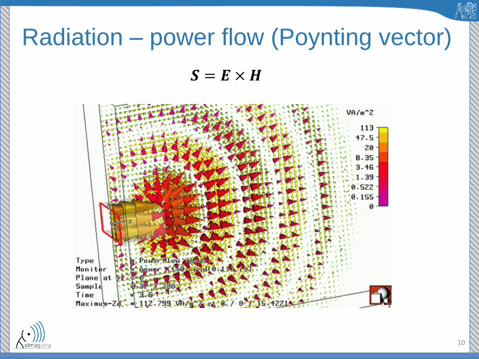
Radiation – power flow (Poynting vector)
10
𝑺 = 𝑬 × 𝑯
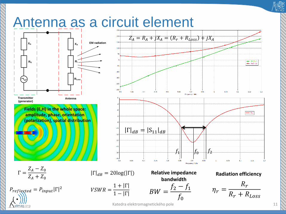
Antenna as a circuit element
Katedra elektromagnetického pole 11
𝑓2 𝑓1 𝑓0
Γ 𝑑𝐵 = S11 𝑑𝐵
𝑍𝐴 = 𝑅𝐴 + 𝑗𝑋𝐴 = 𝑅𝑟 + 𝑅𝐿𝑜𝑠𝑠 + 𝑗𝑋𝐴 XA
Rr
RLoss
XG
RG
Transmitter
(generator)Antenna
EM radiation
Γ =𝑍𝐴 − 𝑍0𝑍𝐴 + 𝑍0
Γ 𝑑𝐵 = 20log( Γ )
𝑃𝑟𝑒𝑓𝑙𝑒𝑐𝑡𝑒𝑑 = 𝑃𝑖𝑛𝑝𝑢𝑡 Γ2 𝑉𝑆𝑊𝑅 =
1 + Γ
1 − Γ 𝐵𝑊 =
𝑓2 − 𝑓1𝑓0
Fields (E,H) in the whole space: amplitude, phase, orientation (polarization), spatial distribution
Relative impedance bandwidth
𝜂𝑟 =𝑅𝑟
𝑅𝑟 + 𝑅𝐿𝑜𝑠𝑠
Radiation efficiency
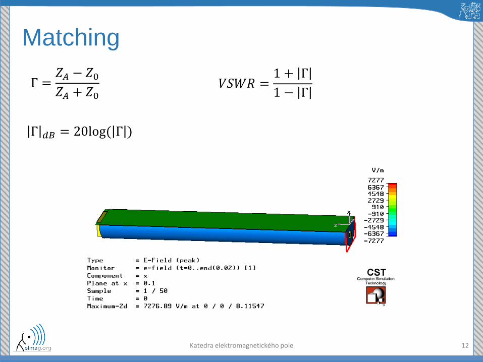
Matching
Katedra elektromagnetického pole 12
Γ 𝑑𝐵 = S11 𝑑𝐵
Γ =𝑍𝐴 − 𝑍0𝑍𝐴 + 𝑍0
Γ 𝑑𝐵 = 20log( Γ )
𝑉𝑆𝑊𝑅 =1 + Γ
1 − Γ
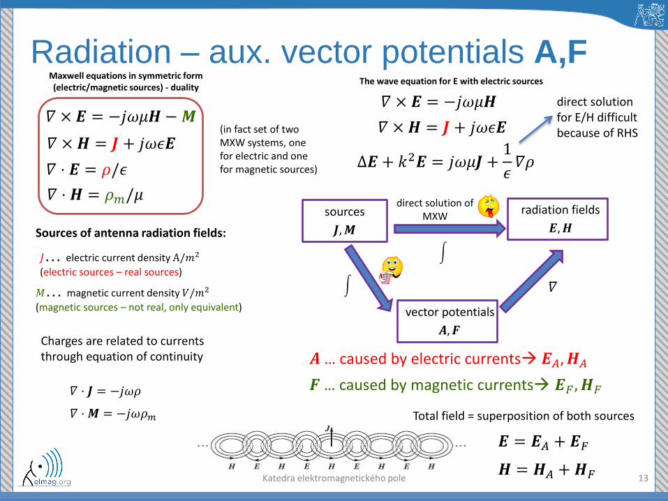
Radiation – aux. vector potentials A,F
Katedra elektromagnetického pole 13
𝛻 × 𝑬 = −𝑗𝜔𝜇𝑯 −𝑴
𝛻 × 𝑯 = 𝑱 + 𝑗𝜔𝜖𝑬
𝛻 ⋅ 𝑬 = 𝜌/𝜖
𝛻 ⋅ 𝑯 = 𝜌𝑚/𝜇
Maxwell equations in symmetric form (electric/magnetic sources) - duality
𝑀… magnetic current density 𝑉/𝑚2
(magnetic sources – not real, only equivalent)
Sources of antenna radiation fields:
𝐽… electric current density A/𝑚2
(electric sources – real sources)
𝛻 ⋅ 𝑱 = −𝑗𝜔𝜌
𝛻 ⋅ 𝑴 = −𝑗𝜔𝜌𝑚
Charges are related to currents through equation of continuity
sources
𝑱,𝑴
radiation fields
𝑬,𝑯
vector potentials
𝑨, 𝑭
direct solution of MXW
𝛻
𝛻 × 𝑬 = −𝑗𝜔𝜇𝑯
𝛻 × 𝑯 = 𝑱 + 𝑗𝜔𝜖𝑬
The wave equation for E with electric sources
∆𝑬 + 𝑘2𝑬 = 𝑗𝜔𝜇𝑱 +1
𝜖𝛻𝜌
𝑨 … caused by electric currents 𝑬𝐴, 𝑯𝐴
𝑭 … caused by magnetic currents 𝑬𝐹 , 𝑯𝐹
(in fact set of two MXW systems, one for electric and one for magnetic sources)
𝑬 = 𝑬𝐴 + 𝑬𝐹
𝑯 = 𝑯𝐴 +𝑯𝐹
direct solution for E/H difficult because of RHS
Total field = superposition of both sources
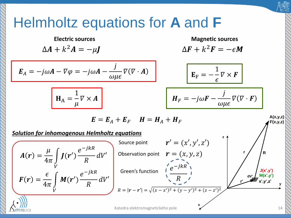
Helmholtz equations for A and F
Katedra elektromagnetického pole 14
∆𝑨 + 𝑘2𝑨 = −𝜇𝑱
𝑯𝐹 = −𝑗𝜔𝑭 −𝑗
𝜔𝜇𝜖𝛻 𝛻 ⋅ 𝑭
∆𝑭 + 𝑘2𝑭 = −𝜖𝑴
𝑬𝐴 = −𝑗𝜔𝑨 − 𝛻𝜑 = −𝑗𝜔𝑨 −𝑗
𝜔𝜇𝜖𝛻 𝛻 ⋅ 𝑨
𝐇A =1
𝜇𝛻 × 𝑨
𝐄F = −1
𝜖𝛻 × 𝑭
Electric sources Magnetic sources
𝑨 𝒓 =𝜇
4𝜋 𝑱(𝒓′)
𝑒−𝑗𝑘𝑅
𝑅𝑑𝑉′
𝑉
𝑬 = 𝑬𝐴 + 𝑬𝐹 𝑯 = 𝑯𝐴 +𝑯𝐹
Solution for inhomogenous Helmholtz equations
𝑭 𝒓 =𝜖
4𝜋 𝑴(𝒓′)
𝑒−𝑗𝑘𝑅
𝑅𝑑𝑉′
𝑉
z
x
y
r R
r’
A(x,y,z)
F(x,y,z)
x’,y’,z’
J(x’,y’)
M(x’,y’)dV’
𝒓 = (𝑥, 𝑦, 𝑧)
𝒓′ = (𝑥′, 𝑦′, 𝑧′) Source point
Observation point
Green’s function 𝑒−𝑗𝑘𝑅
𝑅
𝑅 = 𝒓 − 𝒓′ = 𝑥 − 𝑥′ 2 + 𝑦 − 𝑦′ 2 + 𝑧 − 𝑧′ 2
Elementary electric dipole
Katedra elektromagnetického pole 15
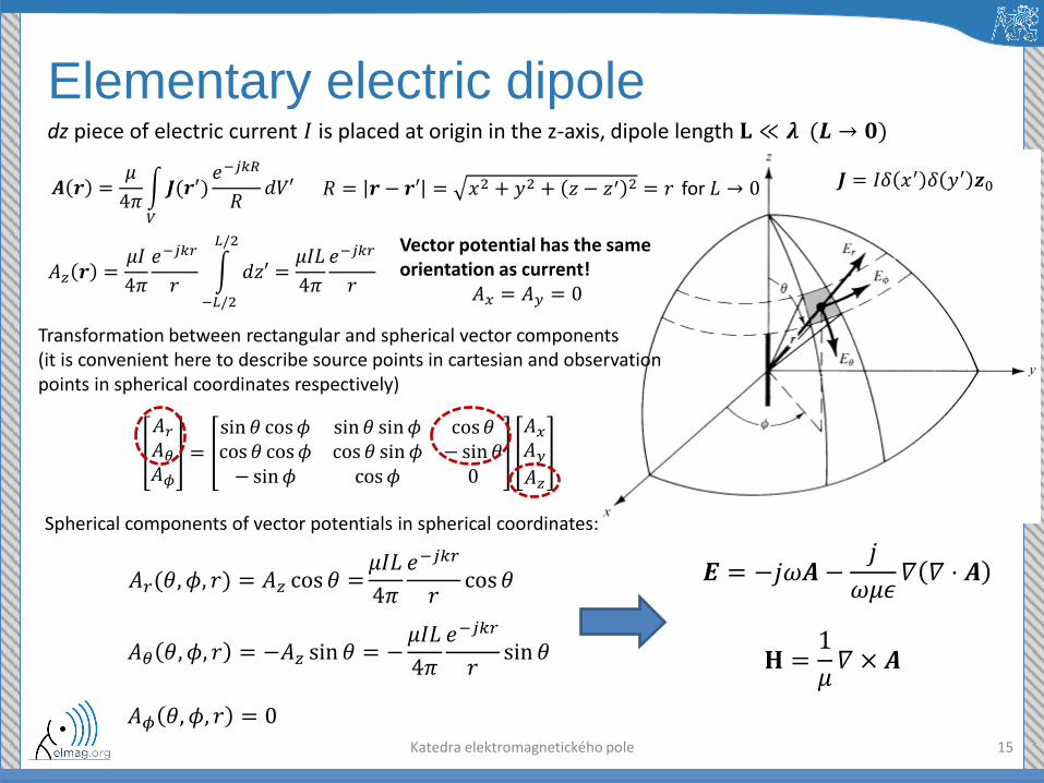
dz piece of electric current 𝐼 is placed at origin in the z-axis, dipole length 𝐋 ≪ 𝝀(𝑳 → 𝟎)
𝑨 𝒓 =𝜇
4𝜋 𝑱(𝒓′)
𝑒−𝑗𝑘𝑅
𝑅𝑑𝑉′
𝑉
𝑱 = 𝐼𝛿 𝑥′ 𝛿 𝑦′ 𝒛0
𝐴𝑧 𝒓 =𝜇𝐼
4𝜋
𝑒−𝑗𝑘𝑟
𝑟 𝑑𝑧′
𝐿/2
−𝐿/2
=𝜇𝐼𝐿
4𝜋
𝑒−𝑗𝑘𝑟
𝑟
𝑅 = 𝒓 − 𝒓′ = 𝑥2 + 𝑦2 + 𝑧 − 𝑧′ 2 = 𝑟 for 𝐿 → 0
Transformation between rectangular and spherical vector components (it is convenient here to describe source points in cartesian and observation points in spherical coordinates respectively)
Vector potential has the same orientation as current!
𝐴𝑥 = 𝐴𝑦 = 0
𝐴𝑟𝐴𝜃𝐴𝜙
=
sin 𝜃 cos𝜙 sin 𝜃 sin𝜙 cos𝜃cos 𝜃 cos𝜙 cos 𝜃 sin𝜙 − sin 𝜃− sin𝜙 cos𝜙 0
𝐴𝑥𝐴𝑦𝐴𝑧
Spherical components of vector potentials in spherical coordinates:
𝐴𝑟(𝜃, 𝜙, 𝑟) = 𝐴𝑧 cos 𝜃 =𝜇𝐼𝐿
4𝜋
𝑒−𝑗𝑘𝑟
𝑟cos 𝜃
𝐴𝜃 𝜃, 𝜙, 𝑟 = −𝐴𝑧 sin 𝜃 = −𝜇𝐼𝐿
4𝜋
𝑒−𝑗𝑘𝑟
𝑟sin 𝜃
𝐴𝜙 𝜃, 𝜙, 𝑟 = 0
𝑬 = −𝑗𝜔𝑨 −𝑗
𝜔𝜇𝜖𝛻 𝛻 ⋅ 𝑨
𝐇 =1
𝜇𝛻 × 𝑨
Elementary electric dipole
Katedra elektromagnetického pole 16
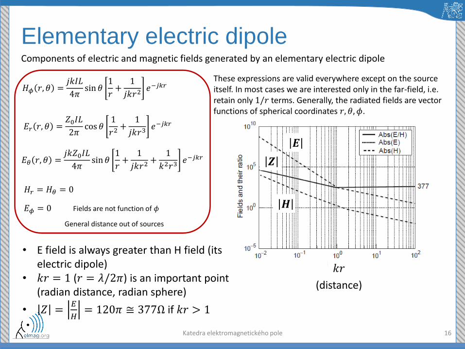
Components of electric and magnetic fields generated by an elementary electric dipole
𝐻𝜙 𝑟, 𝜃 =𝑗𝑘𝐼𝐿
4𝜋sin 𝜃
1
𝑟+1
𝑗𝑘𝑟2𝑒−𝑗𝑘𝑟
𝐻𝑟 = 𝐻𝜃 = 0
𝐸𝜙 = 0
𝐸𝑟 𝑟, 𝜃 =𝑍0𝐼𝐿
2𝜋cos 𝜃
1
𝑟2+1
𝑗𝑘𝑟3𝑒−𝑗𝑘𝑟
𝐸𝜃 𝑟, 𝜃 =𝑗𝑘𝑍0𝐼𝐿
4𝜋sin 𝜃
1
𝑟+1
𝑗𝑘𝑟2+1
𝑘2𝑟3𝑒−𝑗𝑘𝑟
These expressions are valid everywhere except on the source itself. In most cases we are interested only in the far-field, i.e. retain only 1/𝑟 terms. Generally, the radiated fields are vector functions of spherical coordinates 𝑟, 𝜃, 𝜙.
𝑘𝑟
• E field is always greater than H field (its electric dipole)
• 𝑘𝑟 = 1 (𝑟 = 𝜆/2𝜋) is an important point (radian distance, radian sphere)
• 𝑍 = 𝐸
𝐻= 120𝜋 ≅ 377Ω if 𝑘𝑟 > 1
𝑬
𝑯
𝒁
(distance)
General distance out of sources
Fields are not function of 𝜙
Elementary electric dipole
Katedra elektromagnetického pole 17
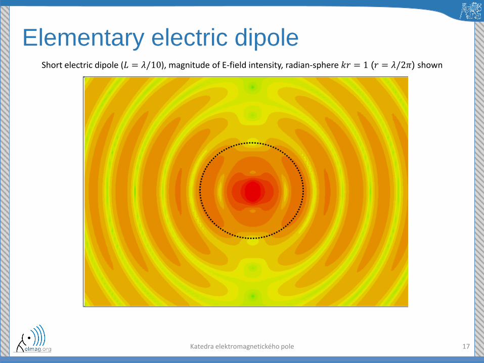
Short electric dipole (𝐿 = 𝜆/10), magnitude of E-field intensity, radian-sphere 𝑘𝑟 = 1 (𝑟 = 𝜆/2𝜋) shown

Elementary electric dipole
18
Oscillating electric dipole consisting of two electric charges in simple harmonic motion, showing propagation of an electric field line and its detachment (radiation) from the dipole
Elementary electric dipole - power
Katedra elektromagnetického pole 19
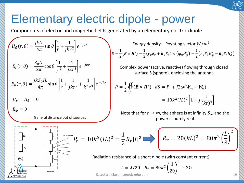
Components of electric and magnetic fields generated by an elementary electric dipole
𝐻𝜙 𝑟, 𝜃 =𝑗𝑘𝐼𝐿
4𝜋sin 𝜃
1
𝑟+1
𝑗𝑘𝑟2𝑒−𝑗𝑘𝑟
𝐻𝑟 = 𝐻𝜃 = 0
𝐸𝜙 = 0
𝐸𝑟 𝑟, 𝜃 =𝑍0𝐼𝐿
2𝜋cos 𝜃
1
𝑟2+1
𝑗𝑘𝑟3𝑒−𝑗𝑘𝑟
𝐸𝜃 𝑟, 𝜃 =𝑗𝑘𝑍0𝐼𝐿
4𝜋sin 𝜃
1
𝑟+1
𝑗𝑘𝑟2+1
𝑘2𝑟3𝑒−𝑗𝑘𝑟
General distance out of sources
𝑺 =1
2𝑬 × 𝑯∗ =
1
2𝒓0𝐸𝑟 + 𝜽0𝐸𝜃 × 𝝓0𝐻𝜙
∗ =1
2𝒓0𝐸𝜃𝐻𝜙
∗ − 𝜽0𝐸𝑟𝐻𝜙∗
Energy density – Poynting vector 𝑊/𝑚2
𝑃 =1
2 𝑬×𝑯∗ ⋅ 𝑑𝑆
𝑆
= 𝑃𝑟 + 𝑗2𝜔 𝑊𝑚 −𝑊𝑒
Complex power (active, reactive) flowing through closed surface S (sphere), enclosing the antenna
= 10𝑘2 𝐼𝐿 2 1 − 𝑗1
𝑘𝑟 3
𝑃𝑟 = 10𝑘2 𝐼𝐿 2 =
1
2𝑅𝑟 𝐼
2 𝑅𝑟 = 20 𝑘𝐿2 = 80𝜋2
𝐿
𝜆
2
Radiation resistance of a short dipole (with constant current)
Note that for 𝑟 → ∞, the sphere is at infinity 𝑆∞ and the power is purely real
𝐿 = 𝜆/20𝑅𝑟 = 80𝜋21
20
2
≅ 2Ω
XA
Rr
RLoss
XG
RG
Transmitter
(generator)Antenna
EM radiation
Elementary electric dipole, field zones
Katedra elektromagnetického pole 20
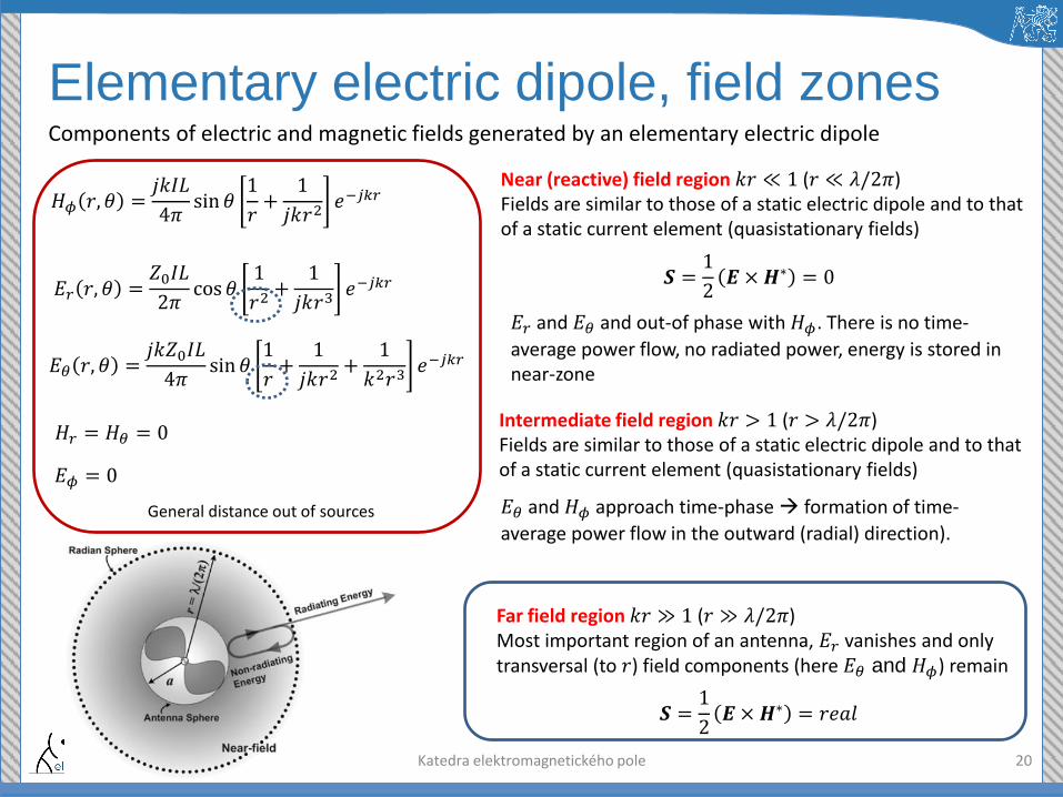
Components of electric and magnetic fields generated by an elementary electric dipole
𝐻𝜙 𝑟, 𝜃 =𝑗𝑘𝐼𝐿
4𝜋sin 𝜃
1
𝑟+1
𝑗𝑘𝑟2𝑒−𝑗𝑘𝑟
𝐻𝑟 = 𝐻𝜃 = 0
𝐸𝜙 = 0
𝐸𝑟 𝑟, 𝜃 =𝑍0𝐼𝐿
2𝜋cos 𝜃
1
𝑟2+1
𝑗𝑘𝑟3𝑒−𝑗𝑘𝑟
𝐸𝜃 𝑟, 𝜃 =𝑗𝑘𝑍0𝐼𝐿
4𝜋sin 𝜃
1
𝑟+1
𝑗𝑘𝑟2+1
𝑘2𝑟3𝑒−𝑗𝑘𝑟
Near (reactive) field region 𝑘𝑟 ≪ 1 (𝑟 ≪ 𝜆/2𝜋) Fields are similar to those of a static electric dipole and to that of a static current element (quasistationary fields)
General distance out of sources
𝑺 =1
2𝑬 ×𝑯∗ = 0
𝐸𝑟 and 𝐸𝜃 and out-of phase with 𝐻𝜙. There is no time-
average power flow, no radiated power, energy is stored in near-zone
Intermediate field region 𝑘𝑟 > 1 (𝑟 > 𝜆/2𝜋) Fields are similar to those of a static electric dipole and to that of a static current element (quasistationary fields)
𝐸𝜃 and 𝐻𝜙 approach time-phase formation of time-
average power flow in the outward (radial) direction).
Far field region 𝑘𝑟 ≫ 1 (𝑟 ≫ 𝜆/2𝜋) Most important region of an antenna, 𝐸𝑟 vanishes and only transversal (to 𝑟) field components (here 𝐸𝜃 and 𝐻𝜙) remain
𝑺 =1
2𝑬 × 𝑯∗ = 𝑟𝑒𝑎𝑙
Elementary electric dipole – FAR FIELD
21
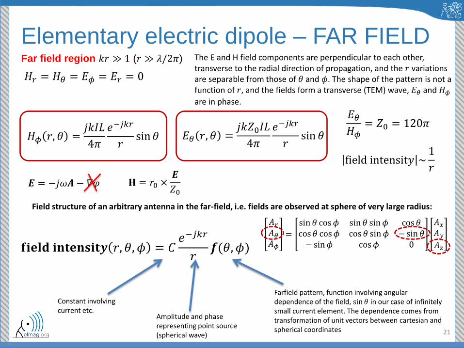
Far field region 𝑘𝑟 ≫ 1 (𝑟 ≫ 𝜆/2𝜋)
𝐻𝜙 𝑟, 𝜃 =𝑗𝑘𝐼𝐿
4𝜋
𝑒−𝑗𝑘𝑟
𝑟sin 𝜃
𝐻𝑟 = 𝐻𝜃 = 𝐸𝜙 = 𝐸𝑟 = 0
𝐸𝜃 𝑟, 𝜃 =𝑗𝑘𝑍0𝐼𝐿
4𝜋
𝑒−𝑗𝑘𝑟
𝑟sin 𝜃
𝐸𝜃𝐻𝜙= 𝑍0 = 120𝜋
Field structure of an arbitrary antenna in the far-field, i.e. fields are observed at sphere of very large radius:
𝐟𝐢𝐞𝐥𝐝𝐢𝐧𝐭𝐞𝐧𝐬𝐢𝐭𝒚 𝑟, 𝜃, 𝜙 = 𝐶𝑒−𝑗𝑘𝑟
𝑟𝒇(𝜃, 𝜙)
Constant involving current etc.
Amplitude and phase representing point source (spherical wave)
fieldintensit𝑦 ~1
𝑟
Farfield pattern, function involving angular dependence of the field, sin 𝜃 in our case of infinitely small current element. The dependence comes from transformation of unit vectors between cartesian and spherical coordinates
𝐴𝑟𝐴𝜃𝐴𝜙
=
sin 𝜃 cos𝜙 sin 𝜃 sin𝜙 cos𝜃cos 𝜃 cos𝜙 cos 𝜃 sin𝜙 − sin 𝜃− sin𝜙 cos𝜙 0
𝐴𝑥𝐴𝑦𝐴𝑧
The E and H field components are perpendicular to each other, transverse to the radial direction of propagation, and the 𝑟 variations are separable from those of 𝜃 and 𝜙. The shape of the pattern is not a function of 𝑟, and the fields form a transverse (TEM) wave, 𝐸𝜃 and 𝐻𝜙
are in phase.
𝑬 = −𝑗𝜔𝑨 − 𝛻𝜑 𝐇 = 𝑟0 ×𝑬
𝑍0
Elementary electric dipole – FAR FIELD
22
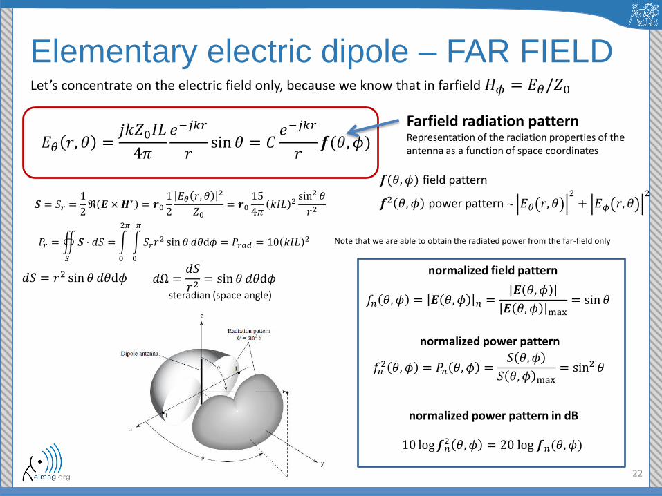
𝐸𝜃 𝑟, 𝜃 =𝑗𝑘𝑍0𝐼𝐿
4𝜋
𝑒−𝑗𝑘𝑟
𝑟sin 𝜃 = 𝐶
𝑒−𝑗𝑘𝑟
𝑟𝒇(𝜃, 𝜙)
Let’s concentrate on the electric field only, because we know that in farfield 𝐻𝜙 = 𝐸𝜃/𝑍0
Farfield radiation pattern Representation of the radiation properties of the antenna as a function of space coordinates
𝒇(𝜃, 𝜙) field pattern
𝒇2 𝜃, 𝜙 power pattern ~ 𝐸𝜃 𝑟, 𝜃2+ 𝐸𝜙 𝑟, 𝜃
2 𝑺 = 𝑆𝒓 =
1
2ℜ 𝑬 × 𝑯∗ = 𝒓0
1
2
𝐸𝜃 𝑟, 𝜃2
𝑍0= 𝒓015
4𝜋𝑘𝐼𝐿 2
sin2 𝜃
𝑟2
𝑃𝑟 = 𝑺 ⋅ 𝑑𝑆
𝑆
= 𝑆𝑟𝑟2 sin 𝜃 𝑑𝜃d𝜙
𝜋
0
2𝜋
0
= 𝑃𝑟𝑎𝑑 = 10 𝑘𝐼𝐿2 Note that we are able to obtain the radiated power from the far-field only
𝑑𝑆 = 𝑟2 sin 𝜃 𝑑𝜃d𝜙 𝑑Ω =𝑑𝑆
𝑟2= sin 𝜃 𝑑𝜃d𝜙
normalized field pattern
𝑓𝑛 𝜃, 𝜙 = 𝑬 𝜃,𝜙 𝑛 =𝑬 𝜃, 𝜙
𝑬 𝜃, 𝜙 max= sin 𝜃
𝑓𝑛2 𝜃, 𝜙 = 𝑃𝑛 𝜃, 𝜙 =
𝑆 𝜃, 𝜙
𝑆 𝜃, 𝜙 max= sin2 𝜃
steradian (space angle)
10 log𝒇𝑛2 𝜃, 𝜙 = 20log𝒇𝑛(𝜃, 𝜙)
normalized power pattern
normalized power pattern in dB

Radiation pattern, directivity
23
Isotropic (point) source, power density 𝑆 = 𝑐𝑜𝑛𝑠𝑡. = 𝑆0
𝑃𝑟 = 𝑆0𝑑𝑆 = 4𝜋𝑟2𝑆0
𝑆
𝑆0 =𝑃𝑟4𝜋𝑟2
𝑈0 = 𝑟2𝑆0 =
𝑃𝑟4𝜋
Radiation intensity 𝑈 is defined as “the power radiated from an antenna per unit space angle (steradian)” and is
related to the far zone E field of an antenna: 𝑈 𝜃,𝜙 =𝑟2
2𝑍0𝑬 𝑟, 𝜃 2.
𝐷 𝜃, 𝜙 =𝑈(𝜃, 𝜙)
𝑈0=𝑈(𝜃, 𝜙)
𝑃𝑟/4𝜋=4𝜋𝑈(𝜃, 𝜙)
𝑃𝑟
Directivity
Isotropic antenna has input power 𝑃𝑖𝑛 = 1W. Radiation intensity is not function of direction,
is constant 𝑈0 =1
4𝜋𝑊/𝑠𝑟
Our source (antenna)
Isotropic source
Directivity = radio of radiation intensity in a given direction from the antenna to the radiation intensity averaged over all directions (isotropic source)
𝐷𝑚𝑎𝑥 = 𝐷 =𝑈𝑚𝑎𝑥𝑈0=4𝜋𝑈𝑚𝑎𝑥𝑃𝑟
=4𝜋
𝑓𝑛2 𝜃, 𝜙 𝑑𝑆
𝑆
Maximum directivity
Elementary electric dipole 𝑓𝑛2 𝜃, 𝜙 = sin2 𝜃
𝐷𝑚𝑎𝑥 =4𝜋
𝑓𝑛2 𝜃,𝜙 𝑑𝑆𝑆
=4𝜋
2𝜋 sin2 𝜃sin𝜃𝑑𝜃𝜋0
=2
4/3=3
2
𝐷𝑑𝐵𝑖 = 10 log 3/2 = 1.76dBi
Effective isotropic radiated power (EIRP)
dBi … decibels over isotropic radiatior
𝐸𝐼𝑅𝑃 = 𝐷 ⋅ 𝑃𝑖𝑛
Antenna with 𝐷 = 30 dBi and 𝑃𝑖𝑛 = 1W
𝐸𝐼𝑅𝑃 = 𝐷 ⋅ 𝑃𝑖𝑛 = 1030
10 ⋅ 1 = 1000 W (equivalent to isotropic source with 𝑃𝑖𝑛 = 𝐸𝐼𝑅𝑃)
Antenna is the best amplifier!!
Antenna efficiency (gain)
24
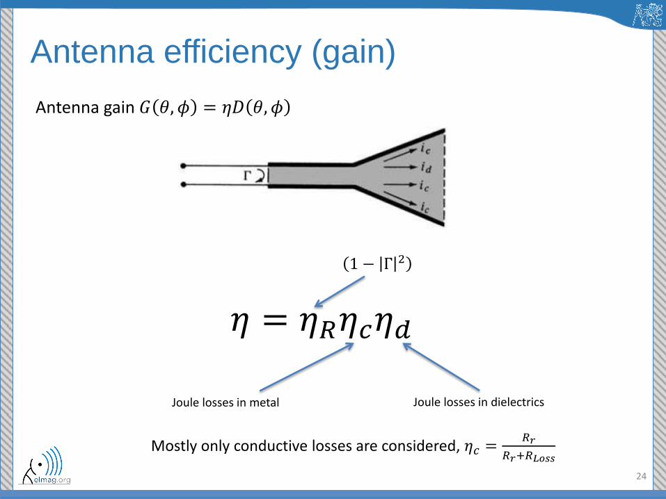
Antenna gain 𝐺 𝜃, 𝜙 = 𝜂𝐷 𝜃, 𝜙
𝜂 = 𝜂𝑅𝜂𝑐𝜂𝑑
1 − Γ 2
Joule losses in metal Joule losses in dielectrics
Mostly only conductive losses are considered, 𝜂𝑐 =𝑅𝑟
𝑅𝑟+𝑅𝐿𝑜𝑠𝑠
Radiation pattern
25
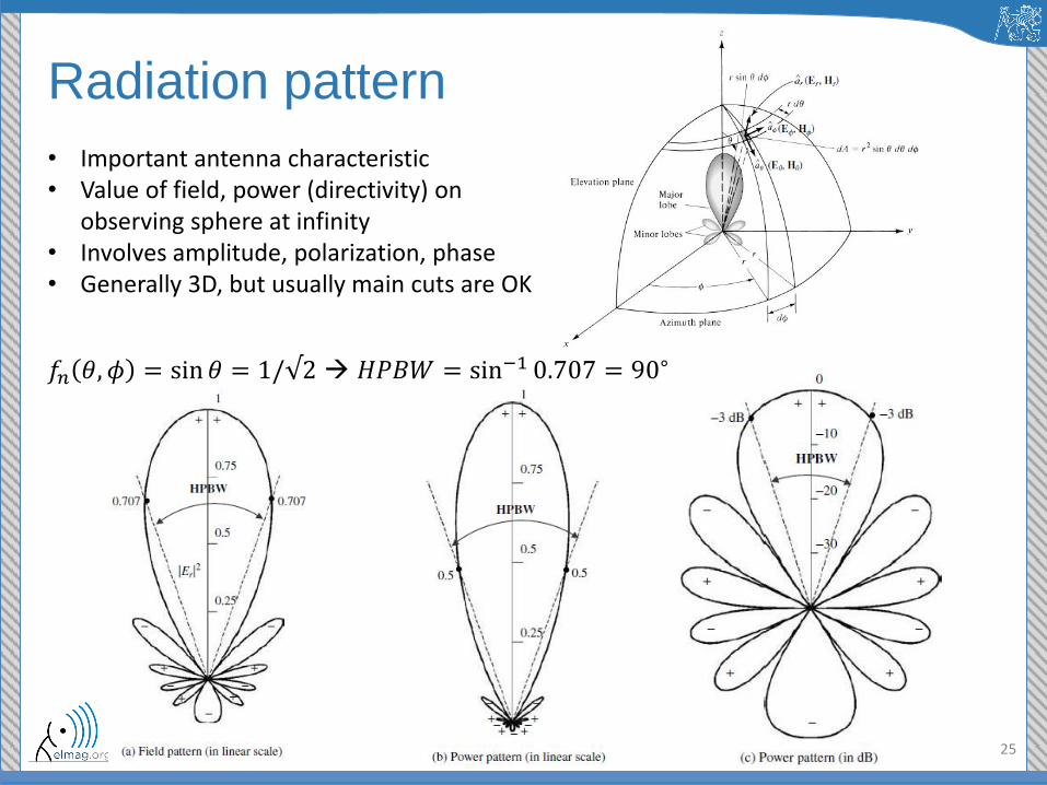
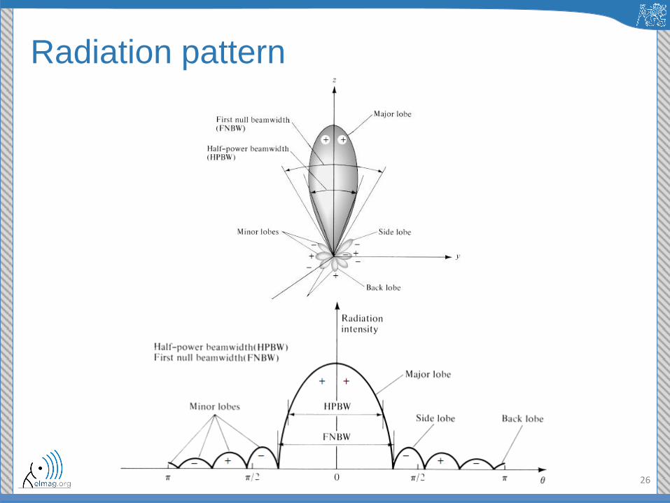
• Important antenna characteristic • Value of field, power (directivity) on
observing sphere at infinity • Involves amplitude, polarization, phase • Generally 3D, but usually main cuts are OK
𝑓𝑛 𝜃, 𝜙 = sin 𝜃 = 1/√2 𝐻𝑃𝐵𝑊 = sin−1 0.707 = 90∘
Radiation pattern
26
Radiation pattern
27
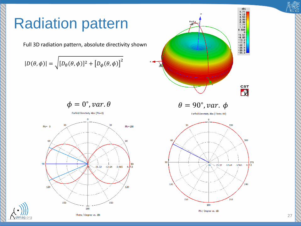
𝜙 = 0∘, 𝑣𝑎𝑟. 𝜃 𝜃 = 90∘, 𝑣𝑎𝑟. 𝜙
Full 3D radiation pattern, absolute directivity shown
𝐷 𝜃, 𝜙 = 𝐷𝜃 𝜃, 𝜙2 + 𝐷𝜙 𝜃, 𝜙
2

Radiation pattern – directional antenna
28
𝐷𝑚𝑎𝑥 = 𝐷 =4𝜋
Ω𝐴≅4𝜋
𝜃1𝑟𝜃2𝑟=41253
𝜃1𝑑𝑒𝑔𝜃2𝑑𝑒𝑔
half-power beamwidths
beam solid angle
Example 𝜃1𝑑𝑒𝑔𝜃2𝑑𝑒𝑔 = 10 ⋅ 10 𝐷𝑚𝑎𝑥 = 412.5, 𝐷𝑑𝐵𝑖 = 26 dBi
Polarization of the radiated field
29
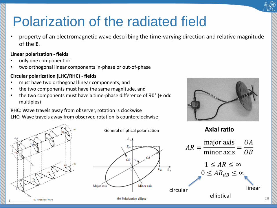
• property of an electromagnetic wave describing the time-varying direction and relative magnitude of the E.
Linear polarization - fields • only one component or • two orthogonal linear components in-phase or out-of-phase
Circular polarization (LHC/RHC) - fields • must have two orthogonal linear components, and • the two components must have the same magnitude, and • the two components must have a time-phase difference of 90∘ (+ odd
multiples)
RHC: Wave travels away from observer, rotation is clockwise LHC: Wave travels away from observer, rotation is counterclockwise
𝐴𝑅 =majoraxis
minoraxis=𝑂𝐴
𝑂𝐵
1 ≤ 𝐴𝑅 ≤ ∞
0 ≤ 𝐴𝑅𝑑𝐵 ≤ ∞
Axial ratio General elliptical polarization
circular elliptical
linear
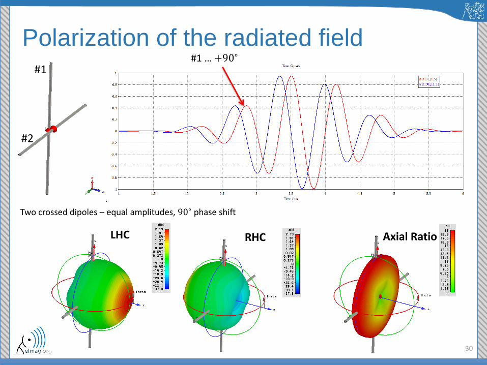
Polarization of the radiated field
30
#1
#2
Two crossed dipoles – equal amplitudes, 90∘ phase shift
#1 … +90∘
LHC RHC Axial Ratio
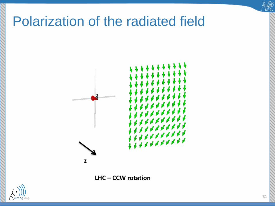
Polarization of the radiated field
31
LHC – CCW rotation
RHC
z
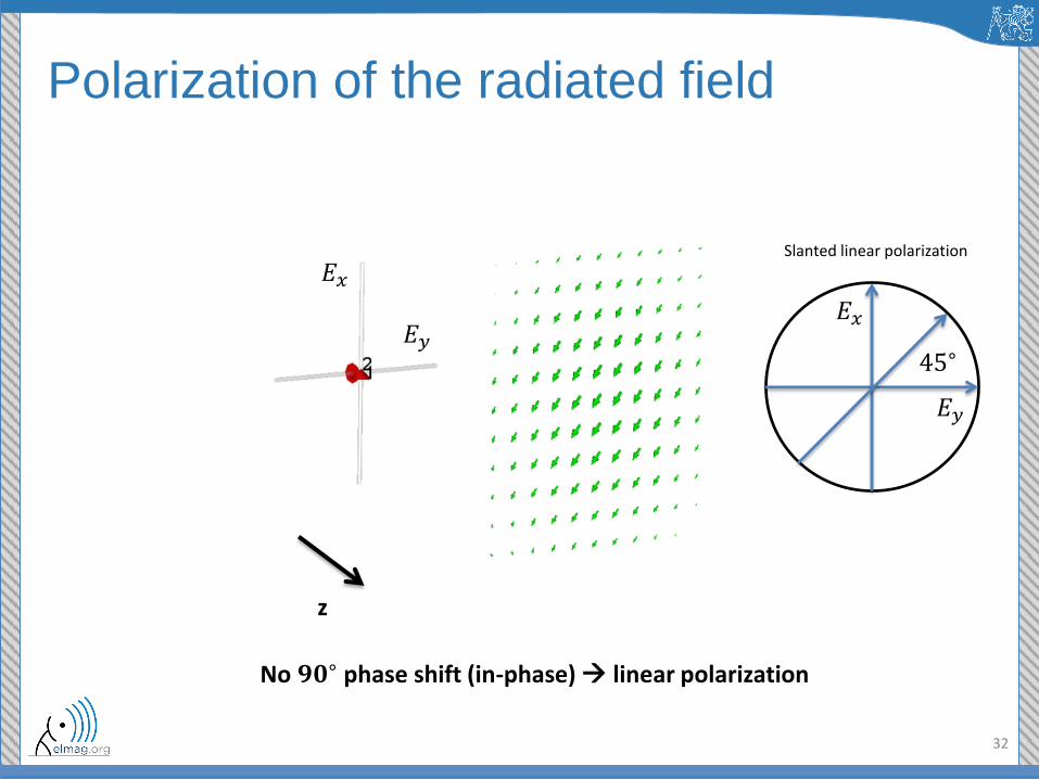
Polarization of the radiated field
32
z
No 𝟗𝟎∘phase shift (in-phase) linear polarization
𝐸𝑥
𝐸𝑦 𝐸𝑥
𝐸𝑦
45∘
Slanted linear polarization

Polarization of the radiated field
33
𝑬
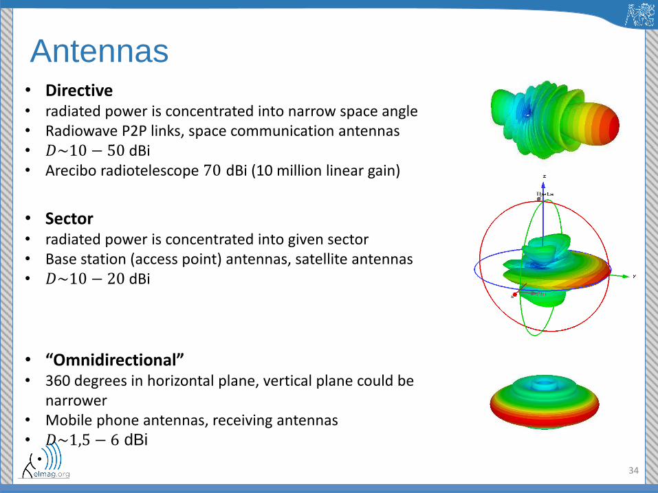
Antennas
34
• Directive • radiated power is concentrated into narrow space angle • Radiowave P2P links, space communication antennas • 𝐷~10 − 50 dBi • Arecibo radiotelescope 70 dBi (10 million linear gain)
• Sector • radiated power is concentrated into given sector • Base station (access point) antennas, satellite antennas • 𝐷~10 − 20 dBi
• “Omnidirectional” • 360 degrees in horizontal plane, vertical plane could be
narrower • Mobile phone antennas, receiving antennas • 𝐷~1,5 − 6 dBi

The “antenna family”
35
• Wire antennas • Straight wire (dipole), loop, helix, …
• Aperture antennas • Horns, reflectors, lens
• Planar (“microstrip” antennas) • Metallic patch on a grounded substrate
• “Special” antennas • fractal geometry, on-chip antennas, mm-wave antennas, metamaterials,
antennas for medical applications (implantable)…
Summary
36
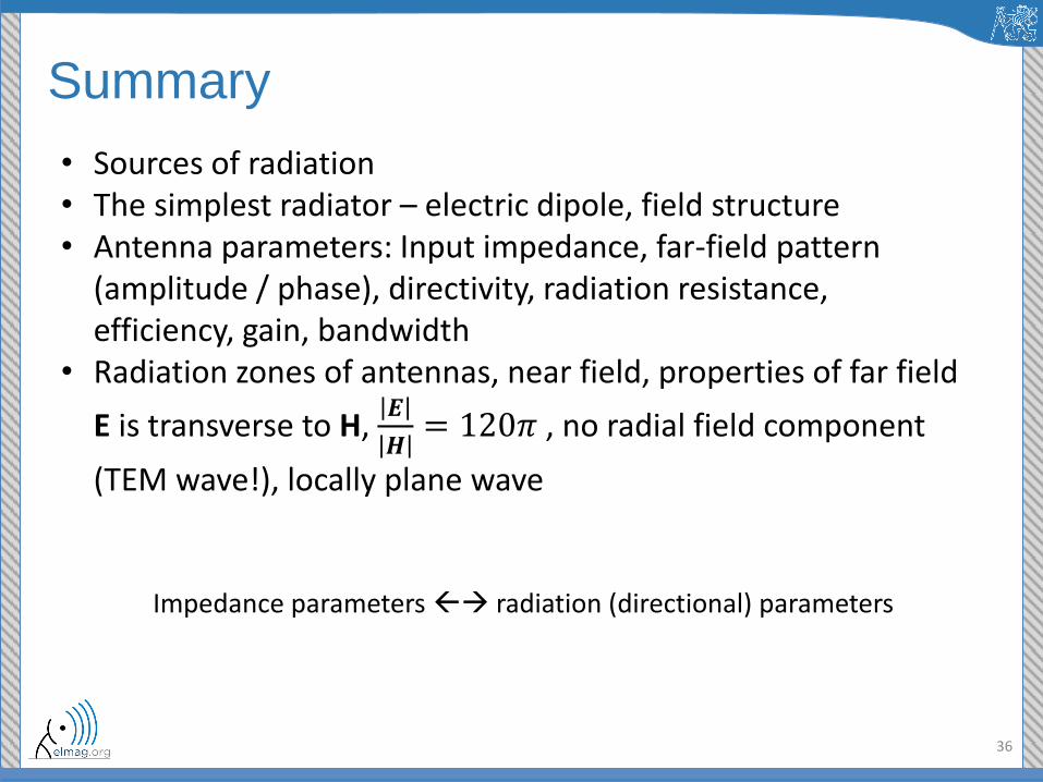
• Sources of radiation • The simplest radiator – electric dipole, field structure • Antenna parameters: Input impedance, far-field pattern
(amplitude / phase), directivity, radiation resistance, efficiency, gain, bandwidth
• Radiation zones of antennas, near field, properties of far field
E is transverse to H, 𝑬
𝑯= 120𝜋 , no radial field component
(TEM wave!), locally plane wave
Impedance parameters radiation (directional) parameters
37
Supplementary material
• Zones of radiation
• Elementary electric dipole – E field during period
• Derivation of potentials
38
Radiation zones
39
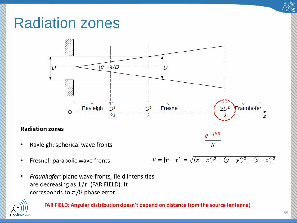
FAR FIELD: Angular distribution doesn’t depend on distance from the source (antenna)
Radiation zones • Rayleigh: spherical wave fronts • Fresnel: parabolic wave fronts • Fraunhofer: plane wave fronts, field intensities
are decreasing as 1/r (FAR FIELD). It corresponds to 𝜋/8 phase error
𝑒−𝑗𝑘𝑅
𝑅
𝑅 = 𝒓 − 𝒓′ = 𝑥 − 𝑥′ 2 + 𝑦 − 𝑦′ 2 + 𝑧 − 𝑧′ 2

Radiation zones
40
Field pattern = function of the radial distance, radial field component may be appreciable.
The angular field distribution is independent of the distance from the
antenna. Field components are transverse
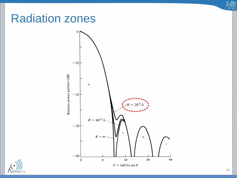
Radiation zones
41

Radiation zones
42
~130λ
Ø 3m
f=1.296 GHz, λ=232 mm
Far field R>78 m (336 λ)
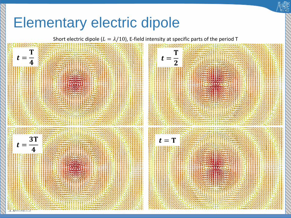
Elementary electric dipole
43
Short electric dipole (𝐿 = 𝜆/10), E-field intensity at specific parts of the period T
𝒕 =𝐓
𝟒 𝒕 =
𝐓
𝟐
𝒕 =𝟑𝐓
𝟒
𝒕 = 𝐓

Vector potential A (similarly for F)
44
Magnetic flux is always solenoidal, so 𝛻 ⋅ 𝑩 = 0 , therefore it can be represented as the curl of another vector 𝛻 ⋅ (𝛻 × 𝑨) = 0 𝑩𝐴 = 𝛻 × 𝑨
𝐇A =1
𝜇𝛻 × 𝑨
𝛻 × 𝑬𝐴 = −𝑗𝜔𝜇𝑯A = −j𝜔𝛻 × 𝑨
First MXW
𝛻 × (𝑬𝐴+𝑗𝜔𝑨) = 0
Can be written as the gradient of some scalar function (potential) 𝜑 since 𝛻 × ∓𝛻𝜑 = 0
𝑬𝐴 + 𝑗𝜔𝑨 = −𝛻𝜑
𝑬𝐴 = −𝑗𝜔𝑨 − 𝛻𝜑 =“solenoidal field+potential field”
Applying 𝛻 ×to both sides of (*) and using identity 𝛻 × 𝛻 × 𝑨 = 𝛻 𝛻 ⋅ 𝑨 − ∆𝑨 leads to wave equation for 𝑨
(*)
∆𝑨 + 𝑘2𝑨 = −𝜇𝑱 + 𝛻 𝛻 ⋅ 𝑨 + 𝑗𝜔𝜇𝜖𝛻𝜑
sign – choosed as in electrostatics
𝛻 ⋅ 𝑨 = −𝑗𝜔𝜇𝜖𝜑 𝛻 𝛻 ⋅ 𝑨 = −𝑗𝜔𝜇𝜖𝛻𝜑
RHS still complicated but we now specify divergence of 𝑨
∆𝑨 + 𝑘2𝑨 = −𝜇𝑱
Such potential calibration (Lorentz gauge) leads to inhomogenous Helmholtz differential equation with simple RHS
𝑬𝐴 = −𝑗𝜔𝑨 − 𝛻𝜑 = −𝑗𝜔𝑨 −𝑗
𝜔𝜇𝜖𝛻 𝛻 ⋅ 𝑨
Using potential calibration, the radiated electric (and magnetic) field is obtained only from knowledge of 𝑨!


![Prof. D. R. Wilton Notes 22 Antennas and Radiation Antennas and Radiation ECE 3317 [Chapter 7]](https://img.pdfslide.us/doc/110x75/56649e935503460f94b98d72/prof-d-r-wilton-notes-22-antennas-and-radiation-antennas-and-radiation-ece.jpg)