Embed Size (px)
Citation preview
Basic Statistics for SGPE Students
Part I: Probability theory1
Mark [email protected]
University of Edinburgh
September 2017
1Thanks to Achim Ahrens, Anna Babloyan and Erkal Ersoy for creatingthese slides and allowing us to use them.
Outline1. Probability theory
I Conditional probabilities and independenceI Bayes’ theorem
2. Probability distributionsI Discrete and continuous probability functionsI Probability density function & cumulative distribution functionI Binomial, Poisson and Normal distributionI E[X] and V[X]
3. Descriptive statisticsI Sample statistics (mean, variance, percentiles)I Graphs (box plot, histogram)I Data transformations (log transformation, unit of measure)I Correlation vs. Causation
4. Statistical inferenceI Population vs. sampleI Law of large numbersI Central limit theoremI Confidence intervalsI Hypothesis testing and p-values
1 / 37
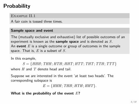
ProbabilityExample II.1A fair coin is tossed three times.
Sample space and eventThe (mutually exclusive and exhaustive) list of possible outcomes of anexperiment is known as the sample space and is denoted as S .An event E is a single outcome or group of outcomes in the samplespace. That is, E is a subset of S .
In this example,S = {HHH ; THH ; HTH ; HHT ; HTT ; THT ; TTH ; TTT}
where H and T denote head and tail.
Suppose we are interested in the event ‘at least two heads’. Thecorresponding subspace is
E = {HHH ; THH ; HTH ; HHT}.
What is the probability of the event E?
2 / 37
ProbabilityLet’s take a step back: What is probability?
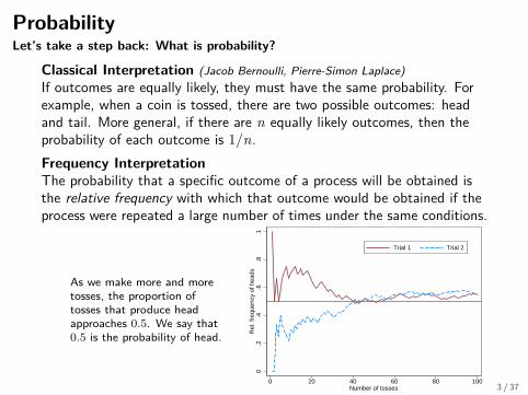
Classical Interpretation (Jacob Bernoulli, Pierre-Simon Laplace)If outcomes are equally likely, they must have the same probability. Forexample, when a coin is tossed, there are two possible outcomes: headand tail. More general, if there are n equally likely outcomes, then theprobability of each outcome is 1/n.Frequency InterpretationThe probability that a specific outcome of a process will be obtained isthe relative frequency with which that outcome would be obtained if theprocess were repeated a large number of times under the same conditions.
As we make more and moretosses, the proportion oftosses that produce headapproaches 0.5. We say that0.5 is the probability of head.
0.2
.4.6
.81
Rel
. fre
quen
cy o
f hea
ds
0 20 40 60 80 100Number of tosses
Trial 1 Trial 2
3 / 37
ProbabilityLet’s take a step back: What is probability?
Subjective Interpretation (Bayesian approach)The probability that a person assigns to a possible outcome represents hisown judgement (based on the person’s beliefs and information). Anotherperson, who may have different beliefs or different information, mayassign a different probability to the same outcome. Distinction betweenprior and posterior beliefs.
Thinking about randomness[Carl Friedrich] Gauss’s conversation turned to chance, the enemy of all
knowledge, and the thing he had always wished to overcome. Viewed fromup close, one could detect the infinite fineness of the web of causality behindevery event. Step back and larger patterns appeared: Freedom and Chancewere a question of distance, a point of view. Did he understand?Sort of, said Eugen wearily, looking at his pocket watch.
from Measuring the World by Daniel Kehlmann
4 / 37
ProbabilityProperties of probability
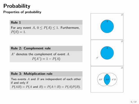
Rule 1For any event A, 0 ≤ P(A) ≤ 1. Furthermore,P(S) = 1.
A
S
Rule 2: Complement ruleAc denotes the complement of event A.
P(Ac) = 1− P(A)
A
Ac
S
Rule 3: Multiplication ruleTwo events A and B are independent of each otherif and only ifP(AB) = P(A and B) = P(A ∩ B) = P(A)P(B).
ABc AB AcB
S
5 / 37
ProbabilityProperties of probability
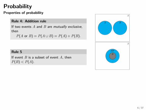
Rule 4: Addition ruleIf two events A and B are mutually exclusive,then
P(A or B) = P(A ∪ B) = P(A) + P(B).
A B
S
Rule 5If event B is a subset of event A, thenP(B) < P(A).
ABc
B
S
6 / 37
ProbabilityWhat is the probability of E?
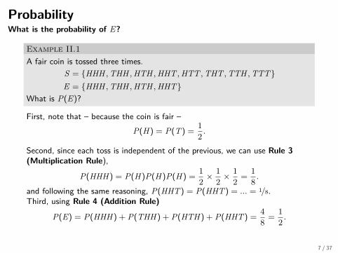
Example II.1A fair coin is tossed three times.
S = {HHH ,THH ,HTH ,HHT ,HTT ,THT ,TTH ,TTT}E = {HHH ,THH ,HTH ,HHT}
What is P(E)?
First, note that – because the coin is fair –
P(H ) = P(T) = 12 .
Second, since each toss is independent of the previous, we can use Rule 3(Multiplication Rule),
P(HHH ) = P(H )P(H )P(H ) = 12 ×
12 ×
12 = 1
8 .
and following the same reasoning, P(HHT) = P(HHT) = ... = 1/8.Third, using Rule 4 (Addition Rule)
P(E) = P(HHH ) + P(THH ) + P(HTH ) + P(HHT) = 48 = 1
2 .
7 / 37
ProbabilityGeneralised addition rule
Example II.2A fair six-sided die is rolled.
The sample space is given by
S = {1, 2, 3, 4, 5, 6}.
Let E1 be the event ‘obtain 3 or 4’ and let E2 denote the event ‘smallerthan 4’. Thus,
E1 = {3, 4} and E2 = {1, 2, 3}
It is immediately clear that P(E1) = 2/6 and P(E2) = 3/6. But what isthe probability that either E1 or E2? That is, what is P(E1 ∪ E2)?
Since E1 and E2 are not mutually exclusive, we cannot apply Rule 4(Addition Rule). But we can generalise Rule 4.
8 / 37
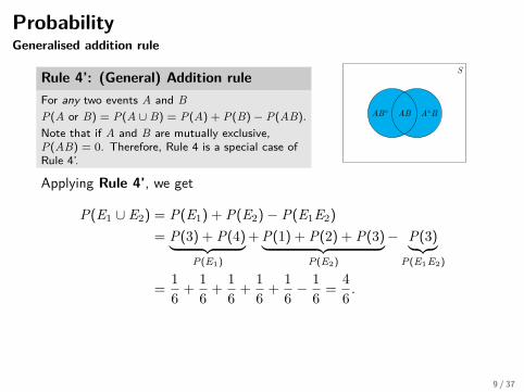
ProbabilityGeneralised addition rule
Rule 4’: (General) Addition ruleFor any two events A and BP(A or B) = P(A ∪ B) = P(A) + P(B)− P(AB).Note that if A and B are mutually exclusive,P(AB) = 0. Therefore, Rule 4 is a special case ofRule 4’.
ABc AB AcB
S
Applying Rule 4’, we get
P(E1 ∪ E2) = P(E1) + P(E2)− P(E1E2)= P(3) + P(4)︸ ︷︷ ︸
P(E1)
+ P(1) + P(2) + P(3)︸ ︷︷ ︸P(E2)
− P(3)︸︷︷︸P(E1E2)
= 16 + 1
6 + 16 + 1
6 + 16 −
16 = 4
6 .
9 / 37
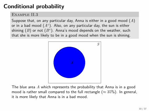
Conditional probabilityExample II.3Suppose that, on any particular day, Anna is either in a good mood (A)or in a bad mood (Ac). Also, on any particular day, the sun is eithershining (B) or not (Bc). Anna’s mood depends on the weather, suchthat she is more likely to be in a good mood when the sun is shining.
A
S
The blue area A which represents the probability that Anna is in a goodmood is rather small compared to the full rectangle (≈ 35%). In general,it is more likely that Anna is in a bad mood.
10 / 37
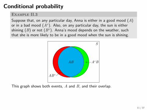
Conditional probabilityExample II.3Suppose that, on any particular day, Anna is either in a good mood (A)or in a bad mood (Ac). Also, on any particular day, the sun is eithershining (B) or not (Bc). Anna’s mood depends on the weather, suchthat she is more likely to be in a good mood when the sun is shining.
ABc −→
AB ←−AcB
S
This graph shows both events, A and B, and their overlap.
11 / 37
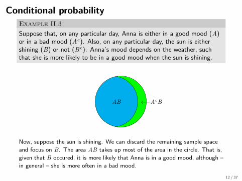
Conditional probabilityExample II.3Suppose that, on any particular day, Anna is either in a good mood (A)or in a bad mood (Ac). Also, on any particular day, the sun is eithershining (B) or not (Bc). Anna’s mood depends on the weather, suchthat she is more likely to be in a good mood when the sun is shining.
AB ←−AcB
Now, suppose the sun is shining. We can discard the remaining sample spaceand focus on B. The area AB takes up most of the area in the circle. That is,given that B occured, it is more likely that Anna is in a good mood, although –in general – she is more often in a bad mood.
12 / 37
Conditional probability
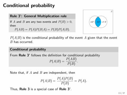
Rule 3’: General Multiplication ruleIf A and B are any two events and P(B) > 0,then
P(AB) = P(A)P(B|A) = P(B)P(A|B).
ABc AB AcB
S
P(A|B) is the conditional probability of the event A given that the eventB has occurred.
Conditional probabilityFrom Rule 3’ follows the definition for conditional probability
P(A|B) = P(AB)P(B) .
Note that, if A and B are independent, then
P(A|B) = P(A)P(B)P(B) = P(A).
Thus, Rule 3 is a special case of Rule 3’.13 / 37
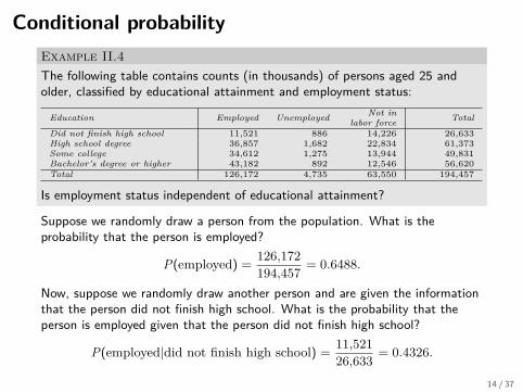
Conditional probabilityExample II.4The following table contains counts (in thousands) of persons aged 25 andolder, classified by educational attainment and employment status:
Education Employed Unemployed Not in Totallabor forceDid not finish high school 11,521 886 14,226 26,633High school degree 36,857 1,682 22,834 61,373Some college 34,612 1,275 13,944 49,831Bachelor’s degree or higher 43,182 892 12,546 56,620Total 126,172 4,735 63,550 194,457
Is employment status independent of educational attainment?
Suppose we randomly draw a person from the population. What is theprobability that the person is employed?
P(employed) = 126,172194,457 = 0.6488.
Now, suppose we randomly draw another person and are given the informationthat the person did not finish high school. What is the probability that theperson is employed given that the person did not finish high school?
P(employed|did not finish high school) = 11,52126,633 = 0.4326.
14 / 37
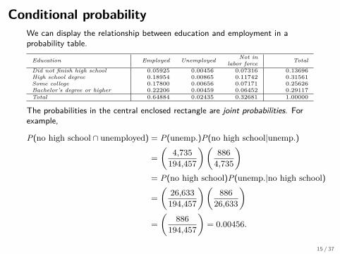
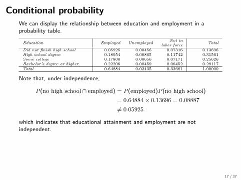
Conditional probabilityWe can display the relationship between education and employment in aprobability table.
Education Employed Unemployed Not in Totallabor forceDid not finish high school 0.05925 0.00456 0.07316 0.13696High school degree 0.18954 0.00865 0.11742 0.31561Some college 0.17800 0.00656 0.07171 0.25626Bachelor’s degree or higher 0.22206 0.00459 0.06452 0.29117Total 0.64884 0.02435 0.32681 1.00000
The probabilities in the central enclosed rectangle are joint probabilities. Forexample,
P(no high school ∩ unemployed) = P(unemp.)P(no high school|unemp.)
=(
4,735194,457
)(8864,735
)= P(no high school)P(unemp.|no high school)
=(
26,633194,457
)(886
26,633
)=(
886194,457
)= 0.00456.
15 / 37
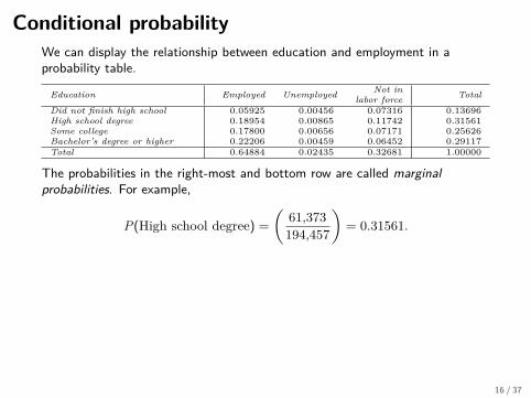
Conditional probabilityWe can display the relationship between education and employment in aprobability table.
Education Employed Unemployed Not in Totallabor forceDid not finish high school 0.05925 0.00456 0.07316 0.13696High school degree 0.18954 0.00865 0.11742 0.31561Some college 0.17800 0.00656 0.07171 0.25626Bachelor’s degree or higher 0.22206 0.00459 0.06452 0.29117Total 0.64884 0.02435 0.32681 1.00000
The probabilities in the right-most and bottom row are called marginalprobabilities. For example,
P(High school degree) =(
61,373194,457
)= 0.31561.
16 / 37
Conditional probabilityWe can display the relationship between education and employment in aprobability table.
Education Employed Unemployed Not in Totallabor forceDid not finish high school 0.05925 0.00456 0.07316 0.13696High school degree 0.18954 0.00865 0.11742 0.31561Some college 0.17800 0.00656 0.07171 0.25626Bachelor’s degree or higher 0.22206 0.00459 0.06452 0.29117Total 0.64884 0.02435 0.32681 1.00000
Note that, under independence,
P(no high school ∩ employed) = P(employed)P(no high school)= 0.64884× 0.13696 = 0.088876= 0.05925.
which indicates that educational attainment and employment are notindependent.
17 / 37
Conditional probability
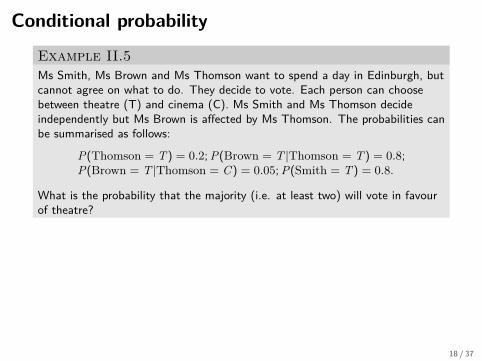
Example II.5Ms Smith, Ms Brown and Ms Thomson want to spend a day in Edinburgh, butcannot agree on what to do. They decide to vote. Each person can choosebetween theatre (T) and cinema (C). Ms Smith and Ms Thomson decideindependently but Ms Brown is affected by Ms Thomson. The probabilities canbe summarised as follows:
P(Thomson = T) = 0.2;P(Brown = T |Thomson = T) = 0.8;P(Brown = T |Thomson = C ) = 0.05;P(Smith = T) = 0.8.
What is the probability that the majority (i.e. at least two) will vote in favourof theatre?
18 / 37
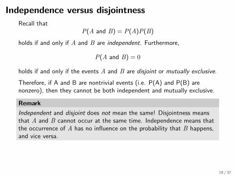
Independence versus disjointnessRecall that
P(A and B) = P(A)P(B)
holds if and only if A and B are independent. Furthermore,
P(A and B) = 0
holds if and only if the events A and B are disjoint or mutually exclusive.
Therefore, if A and B are nontrivial events (i.e. P(A) and P(B) arenonzero), then they cannot be both independent and mutually exclusive.
RemarkIndependent and disjoint does not mean the same! Disjointness meansthat A and B cannot occur at the same time. Independence means thatthe occurrence of A has no influence on the probability that B happens,and vice versa.
19 / 37
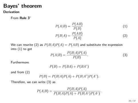
Bayes’ theoremDerivation
From Rule 3’
P(A|B) = P(AB)P(B) (1)
P(B|A) = P(AB)P(A) (2)
We can rewrite (2) as P(B|A)P(A) = P(AB) and substitute the expressioninto (1) to get
P(A|B) = P(B|A)P(A)P(B) . (3)
FurthermoreP(B) = P(BA) + P(BAc)
and from (2)P(B) = P(B|A)P(A) + P(B|Ac)P(Ac).
Therefore, we can write (3) as
P(A|B) = P(B|A)P(A)P(B|A)P(A) + P(B|Ac)P(Ac) .
20 / 37
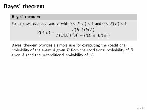
Bayes’ theoremBayes’ theoremFor any two events A and B with 0 < P(A) < 1 and 0 < P(B) < 1
P(A|B) = P(B|A)P(A)P(B|A)P(A) + P(B|Ac)P(Ac)
Bayes’ theorem provides a simple rule for computing the conditionalprobability of the event A given B from the conditional probability of Bgiven A (and the unconditional probability of A).
21 / 37
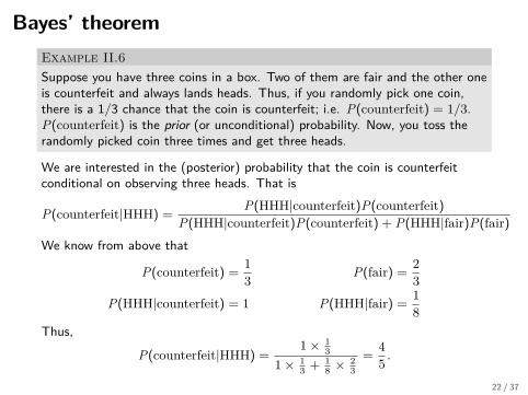
Bayes’ theoremExample II.6Suppose you have three coins in a box. Two of them are fair and the other oneis counterfeit and always lands heads. Thus, if you randomly pick one coin,there is a 1/3 chance that the coin is counterfeit; i.e. P(counterfeit) = 1/3.P(counterfeit) is the prior (or unconditional) probability. Now, you toss therandomly picked coin three times and get three heads.
We are interested in the (posterior) probability that the coin is counterfeitconditional on observing three heads. That is
P(counterfeit|HHH) = P(HHH|counterfeit)P(counterfeit)P(HHH|counterfeit)P(counterfeit) + P(HHH|fair)P(fair)
We know from above that
P(counterfeit) = 13 P(fair) = 2
3
P(HHH|counterfeit) = 1 P(HHH|fair) = 18
Thus,
P(counterfeit|HHH) =1× 1
31× 1
3 + 18 ×
23
= 45 .
22 / 37
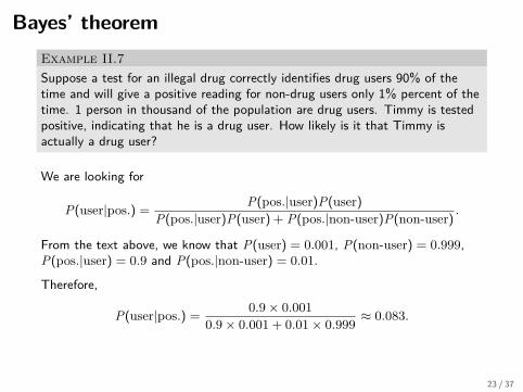
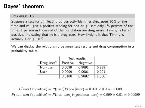
Bayes’ theoremExample II.7Suppose a test for an illegal drug correctly identifies drug users 90% of thetime and will give a positive reading for non-drug users only 1% percent of thetime. 1 person in thousand of the population are drug users. Timmy is testedpositive, indicating that he is a drug user. How likely is it that Timmy isactually a drug user?
We are looking for
P(user|pos.) = P(pos.|user)P(user)P(pos.|user)P(user) + P(pos.|non-user)P(non-user) .
From the text above, we know that P(user) = 0.001, P(non-user) = 0.999,P(pos.|user) = 0.9 and P(pos.|non-user) = 0.01.
Therefore,
P(user|pos.) = 0.9× 0.0010.9× 0.001 + 0.01× 0.999 ≈ 0.083.
23 / 37
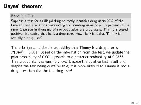
Bayes’ theoremExample II.7Suppose a test for an illegal drug correctly identifies drug users 90% of thetime and will give a positive reading for non-drug users only 1% percent of thetime. 1 person in thousand of the population are drug users. Timmy is testedpositive. indicating that he is a drug user. How likely is it that Timmy isactually a drug user?
The prior (unconditional) probability that Timmy is a drug user isP(user) = 0.001. Based on the information from the test, we update theprior probability of 0.001 upwards to a posterior probability of 0.0833.This probability is surprisingly low. Despite the positive test result anddespite the test being quite reliable, it is more likely that Timmy is not adrug user than that he is a drug user!
24 / 37
Bayes’ theoremExample II.7Suppose a test for an illegal drug correctly identifies drug users 90% of thetime and will give a positive reading for non-drug users only 1% percent of thetime. 1 person in thousand of the population are drug users. Timmy is testedpositive. indicating that he is a drug user. How likely is it that Timmy isactually a drug user?
We can display the relationship between test results and drug consumption in aprobability table:
Test resultsDrug user? Positive NegativeNon-user 0.0099 0.9891 0.999User 0.0009 0.0001 0.001
0.0108 0.9892 1.000
P(user ∩ positive) = P(user)P(pos.|user) = 0.001× 0.9 = 0.0009P(non-user ∩ positive) = P(non-user)P(pos.|non-user) = 0.999× 0.01 = 0.00999
25 / 37
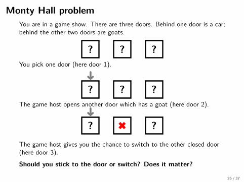
Monty Hall problemYou are in a game show. There are three doors. Behind one door is a car;behind the other two doors are goats.
? ? ?You pick one door (here door 1).
?
Ü
?
Ü
?Ü
The game host opens another door which has a goat (here door 2).
?
Ü
6Ü
?
Ü
The game host gives you the chance to switch to the other closed door(here door 3).
Should you stick to the door or switch? Does it matter?
26 / 37
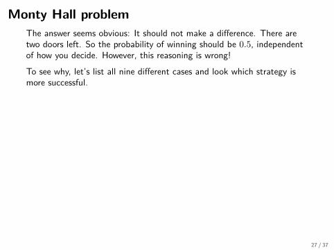
Monty Hall problemThe answer seems obvious: It should not make a difference. There aretwo doors left. So the probability of winning should be 0.5, independentof how you decide. However, this reasoning is wrong!
To see why, let’s list all nine different cases and look which strategy ismore successful.
27 / 37
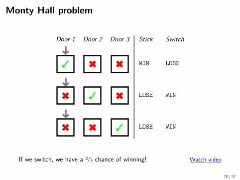
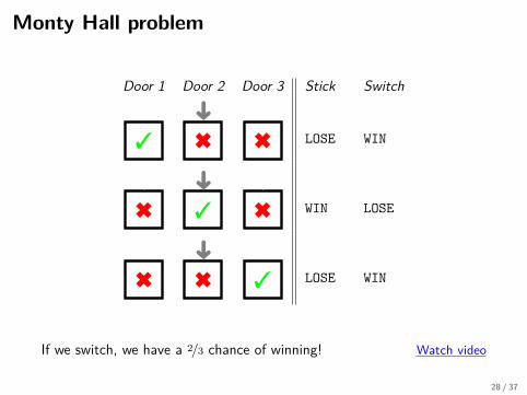
Monty Hall problem
Door 1 Door 2 Door 3 Stick Switch
3
Ü
6
Ü
6
Ü
WIN LOSE
6
Ü
3
Ü
6
Ü
LOSE WIN
6
Ü
6
Ü
3Ü
LOSE WIN
If we switch, we have a 2/3 chance of winning! Watch video
28 / 37
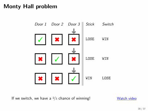
Monty Hall problem
Door 1 Door 2 Door 3 Stick Switch
3
Ü
6
Ü
6
Ü
LOSE WIN
6
Ü
3
Ü
6
Ü
WIN LOSE
6
Ü
6
Ü
3Ü
LOSE WIN
If we switch, we have a 2/3 chance of winning! Watch video
28 / 37
Monty Hall problem
Door 1 Door 2 Door 3 Stick Switch
3
Ü
6
Ü
6
Ü
LOSE WIN
6
Ü
3
Ü
6
Ü
LOSE WIN
6
Ü
6
Ü
3Ü
WIN LOSE
If we switch, we have a 2/3 chance of winning! Watch video
28 / 37
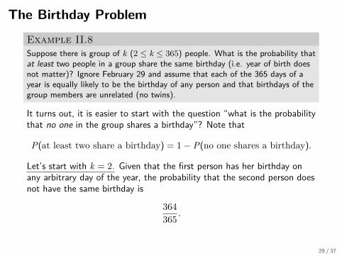
The Birthday Problem
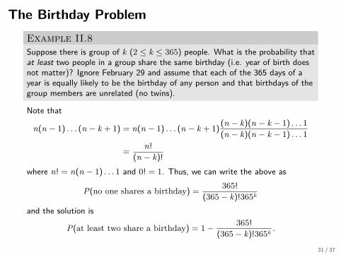
Example II.8Suppose there is group of k (2 ≤ k ≤ 365) people. What is the probability thatat least two people in a group share the same birthday (i.e. year of birth doesnot matter)? Ignore February 29 and assume that each of the 365 days of ayear is equally likely to be the birthday of any person and that birthdays of thegroup members are unrelated (no twins).
It turns out, it is easier to start with the question “what is the probabilitythat no one in the group shares a birthday”? Note that
P(at least two share a birthday) = 1− P(no one shares a birthday).
Let’s start with k = 2. Given that the first person has her birthday onany arbitrary day of the year, the probability that the second person doesnot have the same birthday is
364365 .
29 / 37
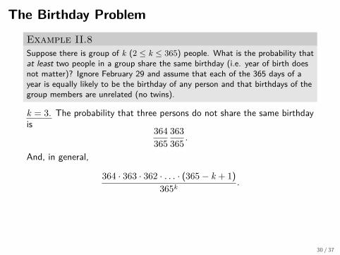
The Birthday Problem
Example II.8Suppose there is group of k (2 ≤ k ≤ 365) people. What is the probability thatat least two people in a group share the same birthday (i.e. year of birth doesnot matter)? Ignore February 29 and assume that each of the 365 days of ayear is equally likely to be the birthday of any person and that birthdays of thegroup members are unrelated (no twins).
k = 3. The probability that three persons do not share the same birthdayis
364365
363365 .
And, in general,
364 · 363 · 362 · . . . · (365− k + 1)365k .
30 / 37
The Birthday ProblemExample II.8Suppose there is group of k (2 ≤ k ≤ 365) people. What is the probability thatat least two people in a group share the same birthday (i.e. year of birth doesnot matter)? Ignore February 29 and assume that each of the 365 days of ayear is equally likely to be the birthday of any person and that birthdays of thegroup members are unrelated (no twins).
Note that
n(n − 1) . . . (n − k + 1) = n(n − 1) . . . (n − k + 1) (n − k)(n − k − 1) . . . 1(n − k)(n − k − 1) . . . 1
= n!(n − k)!
where n! = n(n − 1) . . . 1 and 0! = 1. Thus, we can write the above as
P(no one shares a birthday) = 365!(365− k)!365k
and the solution is
P(at least two share a birthday) = 1− 365!(365− k)!365k .
31 / 37
The Birthday Problem
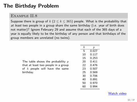
Example II.8Suppose there is group of k (2 ≤ k ≤ 365) people. What is the probability thatat least two people in a group share the same birthday (i.e. year of birth doesnot matter)? Ignore February 29 and assume that each of the 365 days of ayear is equally likely to be the birthday of any person and that birthdays of thegroup members are unrelated (no twins).
The table shows the probability pthat at least two people in a groupof k people will have the samebirthday.
k p5 0.02710 0.11715 0.25320 0.41122 0.47623 0.50725 0.56930 0.70640 0.89150 0.97060 0.994
Watch video
32 / 37
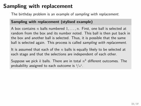
Sampling with replacementThe birthday problem is an example of sampling with replacement.
Sampling with replacement (stylised example)
A box contains n balls numbered 1, . . . , n. First, one ball is selected atrandom from the box and its number noted. This ball is then put back inthe box and another ball is selected. Thus, it is possible that the sameball is selected again. This process is called sampling with replacement.
It is assumed that each of the n balls is equally likely to be selected ateach stage and that the selections are independent of each other.
Suppose we pick k balls. There are in total nk different outcomes. Theprobability assigned to each outcome is 1/nk.
33 / 37
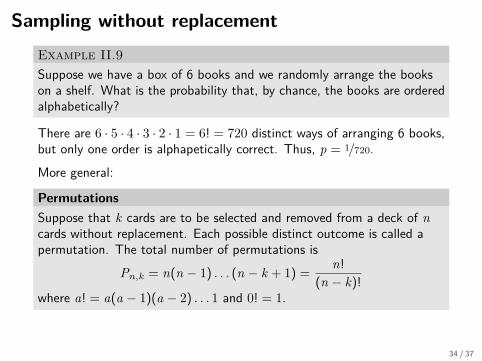
Sampling without replacementExample II.9Suppose we have a box of 6 books and we randomly arrange the bookson a shelf. What is the probability that, by chance, the books are orderedalphabetically?
There are 6 · 5 · 4 · 3 · 2 · 1 = 6! = 720 distinct ways of arranging 6 books,but only one order is alphapetically correct. Thus, p = 1/720.
More general:
PermutationsSuppose that k cards are to be selected and removed from a deck of ncards without replacement. Each possible distinct outcome is called apermutation. The total number of permutations is
Pn,k = n(n − 1) . . . (n − k + 1) = n!(n − k)!
where a! = a(a − 1)(a − 2) . . . 1 and 0! = 1.
34 / 37
Summary
I Frequentist approach: The probability of an outcome is therelative frequency with which that outcome would be obtained if theexperiment were repeated a large number of times.
I Independence and disjointness are not the same! If two events Aand B are mutually exclusive (or disjoint), then P(AB) = 0. If twoevents are independent, then the occurrence of A has no influenceon the probability that B occurs, and vice versa.
I Bayes’ theorem provides a rule for computing the conditionalprobability of the event A given B from the conditional probabilityof B given A. It is the building block of Bayesian econometrics.
35 / 37