BASIC NON-PARAMETRIC STATISTICAL TOOLS*

Prepared for GCMA 2001

Peter M. QuesadaGregory S. Rash

* Examples presented in these notes were obtained from Primer of Biostatistics byStanton S. Glantz (McGraw Hill Text; ISBN: 0070242682)

1

Ordinal Data – Evaluating Two Interventions on Two Different Groups

� Mann-Whitney Rank-Sum Test� Based on ranking of all observations without regard to group associated with each observation� Can also be used with interval or ratio data that are not normally distributed� Test statistic, T, is sum of all ranks for the smaller group

∑=

=Sn

iiRT

1

� where Ri is the rank of the ith observation of the smaller group and nS is the number of observations inthe smaller group

� To determine T must first rank all observations from both groups together� Tied ranks receive average of ranks that would have been spanned (e.g. if 3 observations are tied

following rank 4, then each of the tied observations would receive the average of ranks 5, 6 and 7, or(5+6+7)/2 = 6; the next observation would receive rank 8)

� Critical values of T are based on the tails of the distribution of all possible T values (assuming no ties)

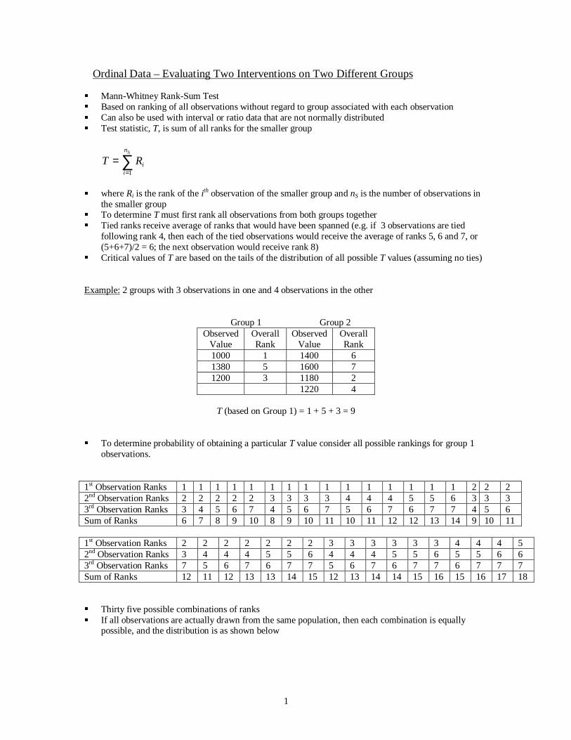
Example: 2 groups with 3 observations in one and 4 observations in the other

Group 1 Group 2Observed

ValueOverallRank

ObservedValue

OverallRank

1000 1 1400 61380 5 1600 71200 3 1180 2

1220 4

T (based on Group 1) = 1 + 5 + 3 = 9

� To determine probability of obtaining a particular T value consider all possible rankings for group 1observations.

1st Observation Ranks 1 1 1 1 1 1 1 1 1 1 1 1 1 1 1 2 2 22nd Observation Ranks 2 2 2 2 2 3 3 3 3 4 4 4 5 5 6 3 3 33rd Observation Ranks 3 4 5 6 7 4 5 6 7 5 6 7 6 7 7 4 5 6Sum of Ranks 6 7 8 9 10 8 9 10 11 10 11 12 12 13 14 9 10 11

1st Observation Ranks 2 2 2 2 2 2 2 3 3 3 3 3 3 4 4 4 52nd Observation Ranks 3 4 4 4 5 5 6 4 4 4 5 5 6 5 5 6 63rd Observation Ranks 7 5 6 7 6 7 7 5 6 7 6 7 7 6 7 7 7Sum of Ranks 12 11 12 13 13 14 15 12 13 14 14 15 16 15 16 17 18

� Thirty five possible combinations of ranks� If all observations are actually drawn from the same population, then each combination is equally

possible, and the distribution is as shown below

2

XX X X X X

X X X X X X XX X X X X X X X X

X X X X X X X X X X X X X6 7 8 9 10 11 12 13 14 15 16 17 18

� If all observations were truly from a single population then there would be a 2/35 = 0.057 (5.7%)probability of obtaining one of the two extreme T values (6 or 18).

� Similarly, there would be a 4/35 = 0.114 (11.4%) probability for a T value ≤ 7 or ≥ 17.� Note that these probabilities are discrete in nature.� In present example T = 9 is associated with probability of 14/35 = 0.4 (40%), which would not be

extreme enough to reject null hypothesis that all observations were drawn from the same population.� When the larger sample contains eight or more observations, distribution of T approximates a normal

distribution with mean

( )2

1++= BSST

nnnµ

where nB is the number of samples in the bigger group, and standard deviation

( )12

1++= BSBST

nnnnθ

� Can then construct test statistic, zT

T

TT

Tz

θµ−=

which can be compared with t-distribution with infinite degrees of freedom (d.o.f.)

� This comparison is more accurate with a continuity correction where

T

T

T

Tz

θ

µ2

1−−=

3

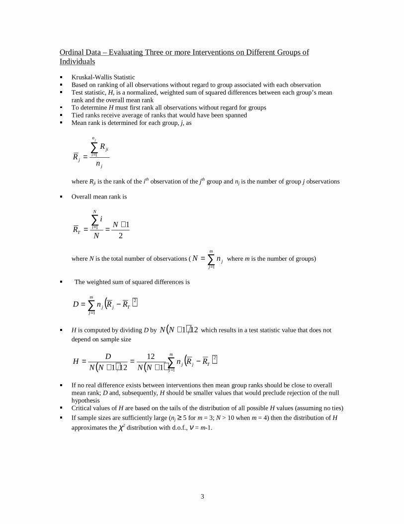
Ordinal Data – Evaluating Three or more Interventions on Different Groups ofIndividuals

� Kruskal-Wallis Statistic� Based on ranking of all observations without regard to group associated with each observation� Test statistic, H, is a normalized, weighted sum of squared differences between each group’s mean

rank and the overall mean rank� To determine H must first rank all observations without regard for groups� Tied ranks receive average of ranks that would have been spanned� Mean rank is determined for each group, j, as

j

n

iji

j n

RR

j

∑== 1

where Rji is the rank of the ith observation of the jth group and nj is the number of group j observations

� Overall mean rank is

2

11 +==∑

= N

N

iR

N

iT

where N is the total number of observations ( ∑=

=m

jjnN

1

where m is the number of groups)

� The weighted sum of squared differences is

( )∑=

−=m

jTjj RRnD

1

2

� H is computed by dividing D by ( ) 121+NN which results in a test statistic value that does notdepend on sample size

( ) ( ) ( )∑=

−+

=+

=m

jTjj RRn

NNNN

DH

1

2

1

12

121

� If no real difference exists between interventions then mean group ranks should be close to overallmean rank; D and, subsequently, H should be smaller values that would preclude rejection of the nullhypothesis

� Critical values of H are based on the tail s of the distribution of all possible H values (assuming no ties)� If sample sizes are suff iciently large (nj ≥ 5 for m = 3; N > 10 when m = 4) then the distribution of H

approximates the χ2 distribution with d.o.f., ν = m-1.

4

Example: 3 groups with different number observations

Group 1 Group 2 Group 3Observed

ValueOverallRank

ObservedValue

OverallRank

ObservedValue

OverallRank

2.04 1 5.30 12 10.36 255.16 10 7.28 19 13.28 296.11 15 9.98 21 11.81 285.82 14 6.59 16 4.54 65.41 13 4.59 8 11.04 263.51 4 5.17 11 10.08 243.18 2 7.25 18 14.47 314.57 7 3.47 3 9.43 234.83 9 7.60 20 13.41 3011.34 273.79 59.03 227.21 17RankSum

146 RankSum

128 RankSum

222

MeanRank

11.23 MeanRank

14.22 MeanRank

24.67

Overall Mean Rank = (31 + 1) / 2 = 16

( ) ( )

( ) ( ) ( ) ( )[ ]201.9107.12

1667.2491622.1491623.111313131

12

1

12

2,01.

222

1

2

=>=

−+−+−+

=

−+

=

=

=∑

νχ

m

jTjj RRn

NNH

� Reject null hypothesis that all observations from a single population� To determine where differences exist perform pair-wise Mann-Whitney tests with Bonferoni

adjustments and continuity corrections.

5

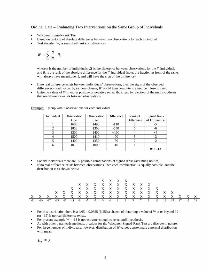
Ordinal Data – Evaluating Two Interventions on the Same Group of Individuals

� Wilcoxon Signed-Rank Test� Based on ranking of absolute differences between two observations for each individual� Test statistic, W, is sum of all ranks of differences

∑= ∆

∆=

n

ii

i

i RW1

where n is the number of individuals, ∆i is the difference between observations for the ith individual,and Ri is the rank of the absolute difference for the ith individual (note: the fraction in front of the rankswill always have magnitude, 1, and will have the sign of the difference)

� If no real difference exists between individuals’ observations, then the signs of the observeddifferences should occur by random chance; W would then compute to a number close to zero.

� Extreme values of W in either positive or negative sense, thus, lead to rejection of the null hypothesisthat no difference exists between observations.

Example: 1 group with 2 observations for each individual

Individual ObservationOne

ObservationTwo

Difference Rank ofDifference

Signed Rankof Difference

1 1600 1490 -110 5 -52 1850 1300 -550 6 -63 1300 1400 +100 4 +44 1500 1410 -90 3 -35 1400 1350 -50 2 -26 1010 1000 -10 1 -1

W = -13

� For six individuals there are 65 possible combinations of signed ranks (assuming no ties).� If no real difference exists between observations, then each combination is equally possible, and the

distribution is as shown below

X X X XX X X X X X X X X X

X X X X X X X X X X X XX X X X X X X X X X X X X X X X

X X X X X X X X X X X X X X X X X X X X X X-21 -19 -17 -15 -13 -11 -9 -7 -5 -3 -1 1 3 5 7 9 11 13 15 17 19 21

� For this distribution there is a 4/65 = 0.0625 (6.25%) chance of obtaining a value of W at or beyond 19(or –19) if no real difference exists.

� For present example W = -13 is not extreme enough to reject null hypothesis.� As with other parametric methods, p-values for the Wilcoxon Signed-Rank Test are discrete in nature.� For large number of individuals, however, distribution of W values approximate a normal distribution

with mean

0=Wµ

6

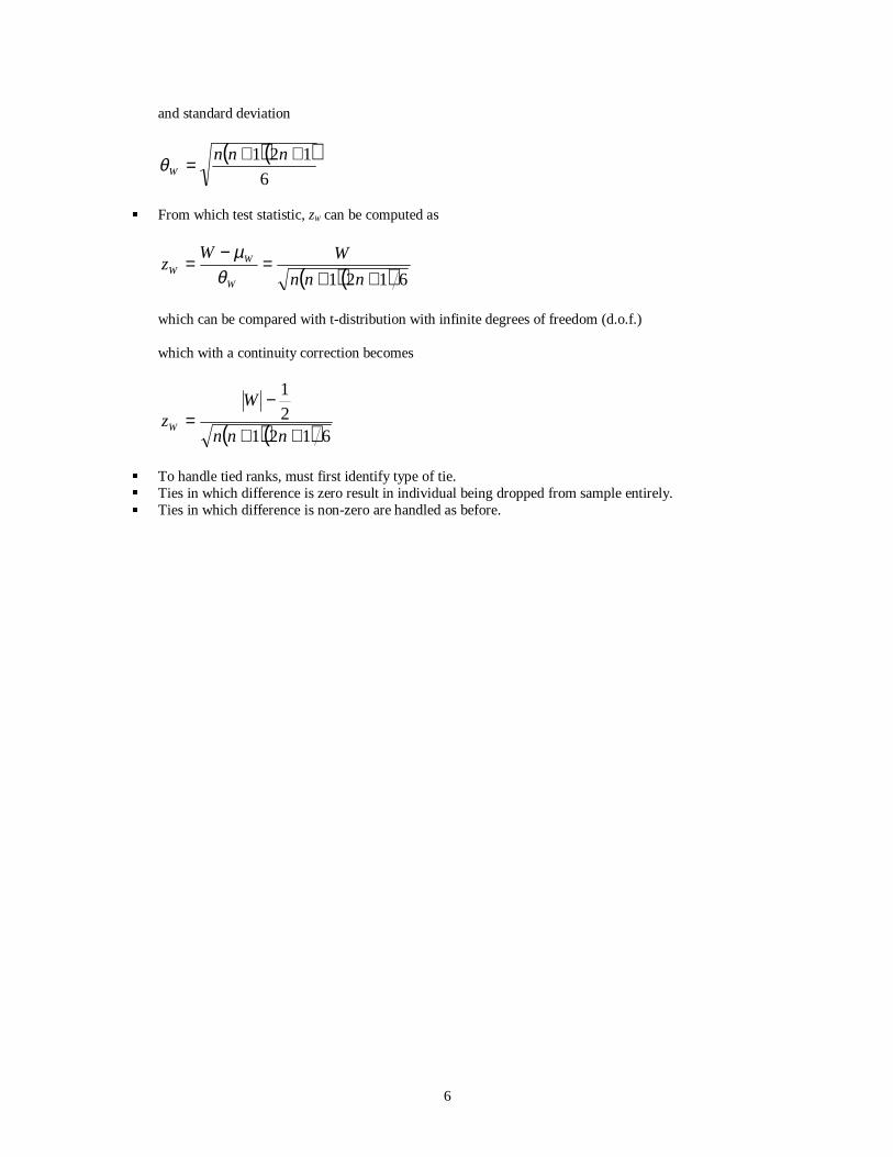
and standard deviation

( )( )6

121 ++= nnnWθ

� From which test statistic, zW can be computed as

( )( ) 6121 ++=

−=

nnn

WWz

W

WW θ

µ

which can be compared with t-distribution with infinite degrees of freedom (d.o.f.)

which with a continuity correction becomes

( )( ) 61212

1

++

−=

nnn

WzW

� To handle tied ranks, must first identify type of tie.� Ties in which difference is zero result in individual being dropped from sample entirely.� Ties in which difference is non-zero are handled as before.

7

Ordinal Data – Evaluating Three or More Interventions on the Same Group of Individuals

� Friedman Statistic� Based on rankings of each individual’s observations associated with each intervention� Initiall y, S is determined as the sum of squared differences between each intervention’s observed rank

sum, ∑=

=n

ijiTj RR

1

, and the expected rank sums, ( ) 21+kn where n is the number of individuals

and k is the number of interventions.

( )( )∑=

+−=k

jTj knRS

1

221

� Friedman statistic is then formed by dividing S by ( ) 121+knk to obtain a statistic whose

distribution approximates a χ2 distribution with ν = k-1.

( )( )( )1

21121

2

2

+

+−=

∑=

knk

knRk

jTj

rχ

� If no real difference exists between individuals’ observations, then observed rank sums should be close

to expected rank sums; thus squared differences should be small, and S & 2rχ should be close to zero.

� If n < 9 for k = 3 or n < 4 for k = 4, distribution of Friedman statistic does not approximate χ2

distribution; must use actual distribution of Friedman statistic to determine discrete criti cal values (seeTable below)

Example: 1 large group with 6 observations for each individual

1st Observation 2nd Observation 3rd Observation 4th Observation 5th Observation 6th ObservationIndividual Value Rank Value Rank Value Rank Value Rank Value Rank Value Rank

1 193 4 217 6 191 3 149 2 202 5 127 12 206 5 214 6 203 4 169 2 189 3 130 13 188 4 197 6 181 3 145 2 192 5 128 14 375 3 412 6 400 5 306 2 387 4 230 15 204 5 199 4 211 6 170 2 196 3 132 16 287 3 310 5 304 4 243 2 312 6 198 17 221 5 215 4 213 3 158 2 232 6 135 18 216 5 223 6 207 3 155 2 209 4 124 19 195 4 208 6 186 3 144 2 200 5 129 110 231 6 224 4 227 5 172 2 218 3 125 1RT 44 53 39 20 49 10

( ) ( )

( )( )( )

( ) ( ) ( ) ( ) ( ) ( )[ ]( )( )( )

515.2063.38

352161021

25,001.

2

2222221

2

2

16610

35103549352035393553354412

1

2112

=>=

=−

=

=+=+

=

=

+

−+−+−+−+−+−

+

+∑

νχχ

χ

r

k

jTj

rknk

knR

kn

• Reject null hypothesis that no difference exists between interventions

8

Example: 1 small group with 3 observations for each individual

1st Observation 2nd Observation 3rd ObservationIndividual Value Rank Value Rank Value Rank

1 22.2 3 5.4 1 10.6 22 17.0 3 6.3 2 6.2 13 14.1 3 8.5 1 9.3 24 17.0 3 10.7 1 12.3 2RT 12 5 7

( ) ( )

( )( )( )

( ) ( ) ( )[ ]( )( )( ) 5.6

1334

8785812

1

2112

8213421

2221

2

2 12 =+

−−−=+

+−=

=+=+

++∑

=

knk

knR

knk

jTj

rχ

• From table below 2rχ matches value with p = .042 for n = 4 and k = 3 ⇒ Reject null hypothesis

k = 3 interventions k = 4 interventionsn 2

rχ p n 2rχ p

3 6.00 .028 2 6.00 .0424 6.50 .042 3 7.00 .054

8.00 .005 8.20 .0175 5.20 .093 4 7.50 .054

6.40 .039 9.30 .0118.40 .008 5 7.80 .049

6 5.33 .072 9.93 .0096.33 .052 6 7.60 .0439.00 .008 10.20 .010

7 6.00 .051 7 7.63 .0518.86 .008 10.37 .009

8 6.25 .047 8 7.65 .0499.00 .010 10.35 .010

9 6.22 .0488.67 .010

10 6.20 .0468.60 .012

11 6.54 .0438.91 .011

12 6.17 .0508.67 .011

13 6.00 .0508.67 .012

14 6.14 .0499.00 .010

15 6.40 .0478.93 .010

9

Ordinal Data – Evaluating Association Between Two Variables

� Spearman Rank Correlation Coefficient� Based on association between rankings of each variable� Initiall y, must rank each variable in either ascending or descending order� Spearman Rank Correlation Coefficient, rS is then essentially determined as the Pearson product-

moment correlation between the ranks, rather than the actual values of the variables.� Alternatively, rS can be computed using the equation

nn

dr

n

ii

S −−=

∑=3

1

261

where di is the difference between variable ranks for the i th individual and n is the number ofindividuals.

� If no real association exists between variables, then the sum of squared differences will t end towardlarger values, and rS will tend toward zero.

� As rS approaches 1, it becomes less li kely that rS value was obtained by random chance for twovariables with no association between them.

� Critical values for rS are identified from Spearman Rank Correlation Coeff icient table depending onacceptable p-value (i.e. chance of falsely concluding that an association exists) and number ofindividuals (samples).

� If n > 50, however, can compute a t-value as

( ) ( )21 2 −−=

nr

rt

S

S

which can be evaluated for significance based on v = n – 2.

Example: Variable 1 Variable 2

Individual Value Rank Value Rank Rank Diff.1 31 1 7.7 2 -12 32 2 8.3 3 -13 33 3 7.6 1 24 34 4 9.1 4 05 35 5.5 9.6 5 0.56 35 5.5 9.9 6 -0.57 40 7 11.8 7 08 41 8 12.2 8 09 42 9 14.8 9 010 46 10 15.0 10 0

( ) ( ) ( )[ ]903.096.0

1010

00005.05.0021161

61

10,001.

3

2222222222

31

2

=>=−

++++−++++−+−−=−

−=

==

∑=

npSS

n

ii

S

rrnn

d

r

• Reject null hypothesis that no association exists between variable 1 and variable 2

10

Probability of Greater Value Pn 0.5 0.2 0.1 0.05 0.02 0.01 0.005 0.002 0.0014 0.600 1.000 1.0005 0.500 0.800 0.900 1.000 1.0006 0.371 0.657 0.829 0.886 0.943 1.000 1.0007 0.321 0.571 0.714 0.786 0.892 0.929 0.964 1.000 1.0008 0.310 0.524 0.643 0.738 0.833 0.881 0.905 0.952 0.9769 0.267 0.483 0.600 0.700 0.783 0.833 0.867 0.917 0.93310 0.248 0.455 0.564 0.648 0.745 0.794 0.830 0.879 0.90311 0.236 0.427 0.536 0.618 0.709 0.755 0.800 0.845 0.87312 0.217 0.406 0.503 0.587 0.678 0.727 0.769 0.818 0.84613 0.209 0.385 0.484 0.560 0.648 0.703 0.747 0.791 0.82414 0.200 0.367 0.164 0.538 0.626 0.679 0.723 0.771 0.80215 0.189 0.354 0.446 0.521 0.604 0.654 0.700 0.75 0.77916 0.182 0.341 0.429 0.503 0.582 0.635 0.679 0.729 0.76217 0.176 0.328 0.414 0.485 0.566 0.615 0.662 0.713 0.74818 0.170 0.317 0.401 0.472 0.550 0.600 0.643 0.695 0.72819 0.165 0.309 0.391 0.460 0.535 0.584 0.628 0.677 0.71220 0.161 0.299 0.380 0.447 0.520 0.570 0.612 0.662 0.69621 0.156 0.292 0.370 0.435 0.508 0.556 0.599 0.648 0.68122 0.152 0.284 0.361 0.425 0.496 0.544 0.586 0.634 0.66723 0.148 0.278 0.353 0.415 0.486 0.532 0.573 0.622 0.65424 0.144 0.271 0.344 0.406 0.476 0.521 0.562 0.610 0.64225 0.142 0.265 0.337 0.398 0.466 0.511 0.551 0.598 0.63026 0.138 0.259 0.331 0.390 0.457 0.501 0.541 0.587 0.61927 0.136 0.255 0.324 0.382 0.448 0.491 0.531 0.577 0.60828 0.133 0.250 0.317 0.375 0.440 0.483 0.522 0.567 0.59829 0.130 0.245 0.312 0.368 0.433 0.475 0.513 0.558 0.58930 0.128 0.240 0.306 0.362 0.425 0.467 0.504 0.549 0.58031 0.126 0.236 0.301 0.356 0.418 0.459 0.496 0.541 0.57132 0.124 0.232 0.293 0.350 0.402 0.452 0.489 0.533 0.56333 0.121 0.229 0.291 0.345 0.405 0.4446 0.482 0.525 0.55434 0.120 0.225 0.287 0.340 0.399 0.439 0.475 0.517 0.54735 0.118 0.222 0.283 0.335 0.394 0.433 0.468 0.510 0.53936 0.116 0.219 0.279 0.330 0.388 0.427 0.462 0.504 0.53337 0.114 0.216 0.275 0.325 0.383 0.421 0.456 0.497 0.52638 0.113 0.212 0.271 0.210 0.378 0.415 0.450 0.491 0.51939 0.111 0.210 0.267 0.317 0.373 0.410 0.444 0.485 0.51340 0.110 0.207 0.264 0.313 0.368 0.405 0.439 0.479 0.50741 0.108 0.204 0.231 0.309 0.364 0.400 0.433 0.473 0.50142 0.107 0.202 0.257 0.305 0.359 0.395 0.428 0.468 0.49543 0.105 0.199 0.254 0.301 0.355 0.391 0.423 0.463 0.49044 0.104 0.197 0.251 0.298 0.351 0.386 0.419 0.458 0.48445 0.103 0.194 0.248 0.294 0.347 0.382 0.414 0.453 0.47946 0.102 0.192 0.246 0.291 0.343 0.378 0.410 0.448 0.47447 0.101 0.190 0.243 0.288 0.340 0.374 0.405 0.443 0.46948 0.100 0.188 0.240 0.285 0.336 0.370 0.401 0.439 0.46549 0.098 0.186 0.238 0.282 0.333 0.366 0.397 0.434 0.46050 0.097 0.184 0.235 0.279 0.329 0.363 0.393 0.43 0.456

11

Nominal Data – Evaluating Two or More Interventions on Different Groups

Chi-square Analysis of Contingency Based on contingency tables containing cell s with numbers of individuals matching row and column

specifications Two types of contingency tables

Observed (actual) Expected

Chi-Square test statistic, χ2 , is a sum of normalized squared differences between corresponding cell sof observed and expected tables

( )∑∑

= =

−=

n

i

m

j ij

ijij

E

EO

1 1

2

2χ

where i is the row index, j is the column index, Oij is the number of observations in cell ij, Eij is theexpected number of observations in cell ij, n is the number of rows, and m is the number of columns.

The expected number of observations for a given cell i s determined from the row, column and overallobservation totals from the observed table as

T

CRE

jiij =

where Ri is the total number of observations in row i, Cj is the total number observations in column j,and T is the total number of observations in the entire table.

χ2 gets larger as observed table deviates more from expected table If no real difference exists between cell or row conditions, then larger χ2 values are less likely to occur

due to random chance. χ2 values associated with random chance probabiliti es less than a critical value (pcrit) cause rejection of

the null hypothesis. χ2 probabiliti es obtained from table based on d.o.f. (ν)

( )( )11 −−= mnν

When ν = 1 (i.e. for 2 X 2 contingency table), should apply Yates correction such that

∑∑= =

−−

=n

i

m

j ij

ijij

E

EO

1 1

2

2 2

1

χ

Example: 2 outcomes, 3 classifications (groups, interventions)

Observed TableOutcome 1 Outcome 2 Row Totals

Classification 1 14 40 54Classification 2 9 14 23Classification 3 46 42 88Column Totals 69 96 165

12

Expected TableOutcome 1 Outcome 2 Row Totals

Classification 1 (54)(69)/165 = 22.58 (54)(96)/165 = 31.42 54Classification 2 (23)(69)/165 = 9.62 (23)(96)/165 = 13.38 23Classification 3 (88)(69)/165 = 36.8 (88)(96)/165 = 51.2 88Column Totals 69 96 165

( )

( ) ( ) ( ) ( ) ( ) ( )

991.5)2(625.9

2.51

2.5142

8.36

8.3646

38.13

38.1314

62.9

62.99

42.31

42.3140

58.22

58.2214

205.

2

2222222

1 1

2

2

==>=

−+−+−+−+−+−=

−= ∑∑

= =

νχχ

χ

χn

i

m

j ij

ijij

E

EO

• Reject null hypothesis and conclude that there is a difference in outcomes between the classifications• Note that results do not yet indicate where the differences are; only that they exist• Can subdivide contingency table to perform pair-wise comparisons

Example continued:

Observed TableOutcome 1 Outcome 2 Row Totals

Classification 2 9 14 23Classification 3 46 42 88Column Totals 55 56 111

Expected TableOutcome 1 Outcome 2 Row Totals

Classification 2 (23)(55)/111 = 11.40 (23)(56)/111 = 11.60 23Classification 3 (88)(55)/111 = 43.60 (88)(56)/111 = 44.40 88Column Totals 55 56 111

841.3)1(79.0

40.44

2

140.4442

60.43

2

160.4346

60.11

2

160.1114

40.11

2

140.119

2

1

205.

2

2222

2

1 1

2

2

==<=

−−

+

−−

+

−−

+

−−

=

−−

= ∑∑= =

νχχ

χ

χn

i

m

j ij

ijij

E

EO

• Cannot reject null hypothesis, so classifications 2 and 3 are deemed to be a single classification• Classifications 2 and 3 are combined to form a new classification (4) which can then be compared with

classification 1

Observed TableOutcome 1 Outcome 2 Row Totals

Classification 1 14 40 54Classification 4 55 56 111Column Totals 69 96 165

13

Expected TableOutcome 1 Outcome 2 Row Totals

Classification 1 (54)(69)/165 = 22.58 (54)(96)/165 = 31.42 54Classification 4 (111)(55)/165 = 46.42 (88)(56)/165 = 64.58 111Column Totals 69 96 165

635.6)1(390.7

58.64

2

158.6456

42.46

2

142.4655

42.31

2

142.3140

58.22

2

158.2214

2

1

201.

2

2222

2

1 1

2

2

==>=

−−

+

−−

+

−−

+

−−

=

−−

= ∑∑= =

νχχ

χ

χn

i

m

j ij

ijij

E

EO

• Reject null hypothesis, classification 1 differs significantly from the combination of classifications 2 &3

14

Nominal Data – Evaluating Two Interventions on the Same Group of Individuals

McNemar’s Test for Changes Based on cell s in 2 X 2 contingency table that represent individuals with different outcomes for each

intervention (cell that represent similar outcomes for each intervention are ignored) Chi-Square test statistic, χ2 , is sum of normalized squared differences between corresponding

observed and expected table cell s that are not ignored (with ν = 1)

∑

−−

=E

EO2

2 2

1

χ

Expected value for the remaining cell s is computed as the average of the remaining cell s

2∑=

OE

If no real difference exists between interventions, then larger χ2 values are less likely to occur due torandom chance.

χ2 values associated with random chance probabiliti es less than a critical value (pcrit) cause rejection ofthe null hypothesis.

Example: 2 outcomes, 3 classifications (groups, interventions)

Observed TableOutcome 1 Outcome 2

Outcome 1 81 48Outcome 2 23 21

Expected TableOutcome 1 Outcome 2

Outcome 1 (48+23)/2 = 35.5Outcome 2 (48+23)/2 = 35.5

Counts of individuals with outcome 1 for both interventions or outcome 2 for both interventions are

ignored; χ2 calculation based on remaining cell s.

635.6)1(113.8

5.35

2

15.3523

5.35

2

15.3548

2

1

201.

2

22

2

2

2

==>=

−−

+

−−

=

−−

= ∑

νχχ

χ

χij

ijij

E

EO

• Reject null hypothesis and conclude that there is a difference in outcomes between the classifications