Basic Matlab Material

8/4/2019 Basic Matlab Material

http://slidepdf.com/reader/full/basic-matlab-material 1/26

5.The MATLAB Overview:

5.1 What is MATLAB?

MATLAB is a high performance language for technical computing. It integrates

computation, visualization and programming in an easy to use environment where

problems and solutions are expressed in a familiar mathematical notation. Typical uses of

MATLAB include :

Math and computation

Algorithm development

Data Acquisition

Modeling, Simulation and prototyping

Data analysis, exploration and visualization

Scientific and Engineering graphics

Application development, including graphical user interface building

MATLAB is an interactive system whose basic data element is an array that does not

require dimensioning. This allows us to solve many technical computing problems

especially those with matrix and vector formulations, in a fraction of time that it would

take to write a program in a scalar non-interactive language such as C or Fortran.

The name MATLAB stands for matrix laboratory. MATLAB was originally written

to provide easy access to matrix software developed by LINPACK and EISPACK

projects. Today MATLAB engines incorporate the LAPACK and BLAS libraries,

embedding the state of art in software for matrix computation.

MATLAB has evolved over a period of years with the input from many users. In

university environments it is the standard instructional tool for introductory and advanced

courses in mathematics, engineering and science. In industry, MATLAB is the tool of

choice for high productivity research, development and analysis.



MATLAB features a family of add-on application specific solutions called toolboxes.

Very important to most users of MATLAB, toolboxes allow one to learn and apply

specialized technology. Toolboxes are comprehensive collection of MATLAB

functions(m-files) that extend the MATLAB environment to solve particular classes of

problems. Areas in which toolboxes are available include signal processing, control

systems, neural networks, fuzzy logic, wavelets, simulation and many others.

5.1.1 The MATLAB system

The MATLAB system consists of three main parts:

5.1.2 Desktop tools and development environment

This is the set of tools and facilities that help us to use MATLAB functions and files.

Many of these tools are graphical user interfaces. It includes the MATLAB desktop and

command window, a command history, an editor and debugger, a code analyzer and other

reports, browsers for viewing help, the workspace, files and the search path.

5.1.3. The MATLAB mathematical function library

This is a vast collection of computational algorithms ranging from elementary functions

like sum, sine, cosine &complex arithmetic, to more sophisticated functions like matrix

inverse, matrix eigen values, Bessel functions and fast fourier transforms.

5.1.4. The MATLAB language

This is a high level matrix language with control flow statements, functions data

structures, input-output, and object oriented programming features. It allows both

“programming in the small” to rapidly create quick and dirty throw-away programs,

and “ programming in the large” to create large and complex application programs.

5.1.5 Graphics

MATLAB has extensive facilities for displaying vectors and matrices as graphs, as well

as annotating and printing these graphs. It includes high-level functions for two-



dimensional data visualization, image processing, animation and presentation graphics. It

also includes low-level functions that allow us to fully customize the appearance of

graphics we well as to build complete graphical interfaces on our MATLAB applications.

5.1.6. The MATLAB External Interfaces/API

This is the library that allows us to write C and Fortran programs that interests with the

MATLAB. It includes facilities for calling routines from MATLAB( dynamic linking),

calling MATLAB as a computational engine and for reading and writing MAT – files.

5.2 Starting and Quitting MATLAB

5. 2.1.Starting MATLAB

On Windows platforms, start MATLAB by double clicking the MATLAB shortcut icon

on the windows desktop.

On UNIX platforms, start MATLAB by typing matlab at the operating system prompt

5.2.2. MATLAB desktop

when we start MATLAB, the MATLAB desktop appears, containing tools for managing

files, variables and applications associated with MATLAB. The typical schematic of the

MATLAB desktop is as follows:

5.2.3 Command Window

We use this part of the Desktop to write the executable code of the program. Any

program no matter wherever it is written it is executed in the command window.

5.2.4 Current Directory



It holds the list of variables, files and folders which are used in the execution of the

current program.

5.2.5 Workspace

Whenever any executable code is written the files are saved and the default location for

saving the files is the workspace of the MATLAB. It holds the files that are saved in the

current execution.

5. 2.6 Command History

It holds the history of all the statements that were recently executed on the command

window. It holds the contents of the statements until the command history is cleared.

5.2.7 M files

These are the normal editor files which are used to write any executable MATLAB code

before it is imported into the command window for execution.

Comma

nd

window

View or change the

current directoryCurrent directory

workspace

Command history



5.2.8 Figure Window

This window is used to display the figures and plots of the results in MATLAB command

window. A detailed discussion on plotting functions is discussed in the further chapters.

5.2.9 . Quitting MATLAB

To end the MATLAB session, select File>Exit MATLAB in the desktop or type quit

in the command window. We can run a script file named finish.m each time MATLAB

quits that for example, executes functions to save the workspace.

Confirm quitting

MATLAB can display a confirmation dialog box before quitting. To set this option,

select File>Preferences>General>Confirmation Dailogs, and select the check box for

confirm before exiting MATLAB.

5.3 MATRICES and ARRAYS

In MATLAB, a matrix is a rectangular array of numbers. Sometimes there is some

special significance attached to 1-by-1 matrices, which are scalars, and to matrices with

only one row or column, which are vectors. MATLAB has other ways of storing both

numeric and non numeric data, but in the beginning, it is usually best to think of

everything as a matrix. The operations in MATLAB are designed to be as natural as

possible. Unlike the other programming languages which work with numbers one at a

time, MATLAB allows us to work with entire matrices quickly and easily.



5.3.1 Matrix Indices:

4.3.1.1 Entering the elements into a Matrix

The best way to get started with MATLAB is to learn how to handle the matrices. Start

MATLAB and follow the given examples sequentially:

We can enter the elements into a Matrix in several ways:

• Enter the explicit list of elements.

• Load matrices from external data files.

• Generate matrices using the built-in functions

• Create matrices with own functions like the M-files.

First let us create the matrix by explicitly entering the elements,

• Separate the elements of a row with either the blanks or commas,

• Use a semicolon, ; , to indicate the end of each row,

• Surround the entire list of elements by the square braces, [ ].

To enter the elements into the matrix, simply type the following in the command window,

For example:

A= [ 1 2 3; 4 5 6 ; 7 8 9] or A = [ 1,2,3; 4,5,6; 7,8,9]

Now the MATLAB displays the matrix we just entered as :

A = 1 2 3

4 5 6

7 8 9



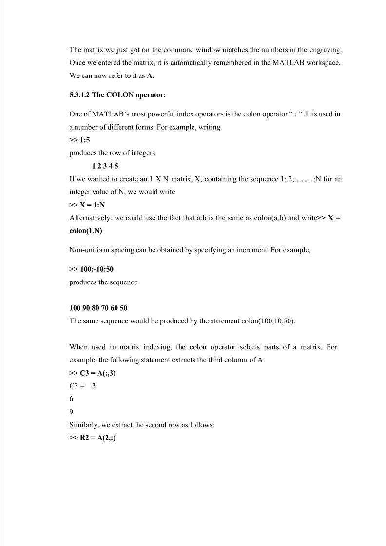
The matrix we just got on the command window matches the numbers in the engraving.

Once we entered the matrix, it is automatically remembered in the MATLAB workspace.

We can now refer to it as A.

5.3.1.2 The COLON operator:

One of MATLAB’s most powerful index operators is the colon operator “ : ” .It is used in

a number of different forms. For example, writing

>> 1:5

produces the row of integers

1 2 3 4 5

If we wanted to create an 1 X N matrix, X, containing the sequence 1; 2; …… ;N for an

integer value of N, we would write

>> X = 1:N

Alternatively, we could use the fact that a:b is the same as colon(a,b) and write>> X =

colon(1,N)

Non-uniform spacing can be obtained by specifying an increment. For example,

>> 100:-10:50

produces the sequence

100 90 80 70 60 50

The same sequence would be produced by the statement colon(100,10,50).

When used in matrix indexing, the colon operator selects parts of a matrix. For

example, the following statement extracts the third column of A:

>> C3 = A(:,3)

C3 = 3

6

9

Similarly, we extract the second row as follows:

>> R2 = A(2,:)



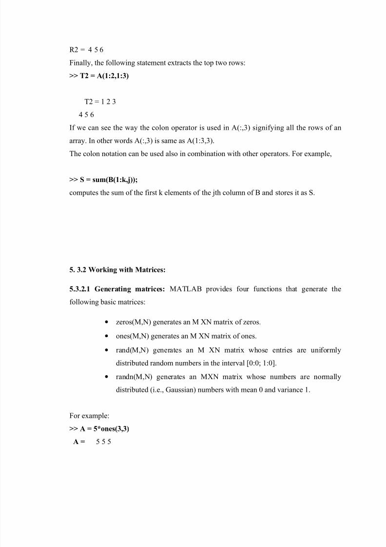
R2 = 4 5 6

Finally, the following statement extracts the top two rows:

>> T2 = A(1:2,1:3)

T2 = 1 2 3

4 5 6

If we can see the way the colon operator is used in A(:,3) signifying all the rows of an

array. In other words A(:,3) is same as A(1:3,3).

The colon notation can be used also in combination with other operators. For example,

>> S = sum(B(1:k,j));

computes the sum of the first k elements of the jth column of B and stores it as S.

5. 3.2 Working with Matrices:

5.3.2.1 Generating matrices: MATLAB provides four functions that generate the

following basic matrices:

• zeros(M,N) generates an M XN matrix of zeros.

• ones(M,N) generates an M XN matrix of ones.

• rand(M,N) generates an M XN matrix whose entries are uniformly

distributed random numbers in the interval [0:0; 1:0].

• randn(M,N) generates an MXN matrix whose numbers are normally

distributed (i.e., Gaussian) numbers with mean 0 and variance 1.

For example:

>> A = 5*ones(3,3)

A = 5 5 5



5 5 5

5 5 5

>> B = rand(2,4)

B = 0.2311 0.4860 0.7621 0.0185

0.6068 0.8913 0.4565 0.8214

>> N =fix(10*rand(1,10))

N = 8 9 1 9 6 0 2 5 9 9

>> R = randn(4,4)

R = -0.4326 -1.1465 0.3273 -0.5883

-1.6656 1.1909 0.1746 2.1832

0.1253 1.1892 -0.1867 -0.1364

0.2877 -0.0376 0.7258 0.1139

5.3.2.2 Matrix Concatenation:

Matrix concatenation is the process of joining small matrices to create larger matrices.

The concatenation operator is the pair of square brackets, [ ].

when we wrote

>> A = [1 2 3;4 5 6;7 8 9]

all we did was concatenate three rows (separated by semicolons) to create a 3x3 matrix.

Note that individual elements are separated by a space. Separating the elements by

commas would yield the same result. The group of three elements before the first

semicolon formed the first row, the next group formed the second row, and so on. Clearly

the number of elements

between semicolons have to be equal. This concept is applicable also when the elements

themselves are matrices. For example, consider the 2X2 matrix



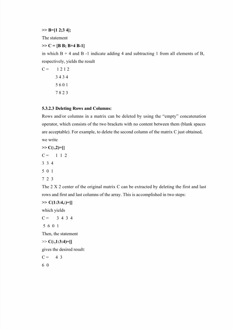
>> B=[1 2;3 4];

The statement

>> C = [B B; B+4 B-1]

in which B + 4 and B -1 indicate adding 4 and subtracting 1 from all elements of B,

respectively, yields the result

C = 1 2 1 2

3 4 3 4

5 6 0 1

7 8 2 3

5.3.2.3 Deleting Rows and Columns:

Rows and/or columns in a matrix can be deleted by using the “empty” concatenation

operator, which consists of the two brackets with no content between them (blank spaces

are acceptable). For example, to delete the second column of the matrix C just obtained,

we write

>> C(:,2)=[]

C = 1 1 2

3 3 4

5 0 1

7 2 3

The 2 X 2 center of the original matrix C can be extracted by deleting the first and last

rows and first and last columns of the array. This is accomplished in two steps:

>> C(1:3:4,:)=[]

which yields

C = 3 4 3 4

5 6 0 1

Then, the statement

>> C(:,1:3:4)=[]

gives the desired result:

C = 4 3

6 0



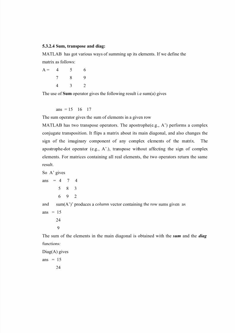
5.3.2.4 Sum, transpose and diag:

MATLAB has got various ways of summing up its elements. If we define the

matrix as follows:

A = 4 5 6

7 8 9

4 3 2

The use of Sum operator gives the following result i.e sum(a) gives

ans = 15 16 17

The sum operator gives the sum of elements in a given row

MATLAB has two transpose operators. The apostrophe(e.g., A’) performs a complex

conjugate transposition. It flips a matrix about its main diagonal, and also changes the

sign of the imaginary component of any complex elements of the matrix. The

apostrophe-dot operator (e.g., A’.), transpose without affecting the sign of complex

elements. For matrices containing all real elements, the two operators return the same

result.

So A’ gives

ans = 4 7 4

5 8 3

6 9 2

and sum(A’)’ produces a column vector containing the row sums given as

ans = 15

24

9

The sum of the elements in the main diagonal is obtained with the sum and the diag

functions:

Diag(A) gives

ans = 15

24



9

And sum(diag(A)) gives

ans = 14

5.3.2.5 The Magic function:

MATLAB actually has a built in function that creates magic squares of almost any size.

Obviously, this function is named as magic:

For example:

B=magic(4);

B = 16 2 3 13

5 11 10 8

9 7 6 12

4 14 15 1

The magic function produces a matrix in which if we sum up all the elements of a row or

a column, they are identical.

5.3.3 Matrices and Arrays:

Informally, the term matrix and array are often used interchangeably. More precisely, a

matrix is a two-dimensional array that represents a linear transformation. The

mathematical operations defined on matrices are subject to linear algebra.

• Adding a matrix to its transpose produces a symmetric matrix

A+A’

ans = 8 12 10

12 16 12

10 12 4

• The matrix multiplication symbol, *, denotes the matrix multiplication involving

inner products between rows and columns. Multiplying the transpose of a matrix

by the original matrix also produces a symmetric matrix.

A’*A



ans =

81 88 95

88 98 108

95 108 121

• If the determinant of the matrix happens to be zero, it is known as a singular

matrix.

Ans = 0

Arrays:

If we come out of the world of linear algebra, matrices become two-dimensional numeric

arrays. Arithmetic operations on arrays are done element by element. This means that

addition and subtraction are same for both arrays and matrices, but when it comes for

multiplicative operations, the things are quite different. MATLAB uses a dot operator as

a part of the notation for the multiplicative array operations.

The list of operators include

+ addition

- Subtraction

.* Element by element multiplication

./ Element by element division

.\ Element by element left division

.^ Element by element power

.’ unconjugated array transpose

For example:

A.*A produces

ans = 16 25 36

49 64 81

16 9 4

The result of the above operation is that the element values of the matrix A are squared.

Building tables:



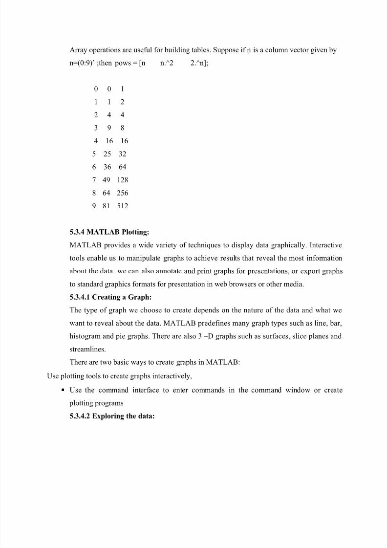
Array operations are useful for building tables. Suppose if n is a column vector given by

n=(0:9)’ ;then pows = [n n.^2 2.^n];

0 0 1

1 1 2

2 4 4

3 9 8

4 16 16

5 25 32

6 36 64

7 49 128

8 64 256

9 81 512

5.3.4 MATLAB Plotting:

MATLAB provides a wide variety of techniques to display data graphically. Interactive

tools enable us to manipulate graphs to achieve results that reveal the most information

about the data. we can also annotate and print graphs for presentations, or export graphs

to standard graphics formats for presentation in web browsers or other media.

5.3.4.1 Creating a Graph:

The type of graph we choose to create depends on the nature of the data and what we

want to reveal about the data. MATLAB predefines many graph types such as line, bar,

histogram and pie graphs. There are also 3 –D graphs such as surfaces, slice planes and

streamlines.

There are two basic ways to create graphs in MATLAB:

Use plotting tools to create graphs interactively,

• Use the command interface to enter commands in the command window or create

plotting programs

5.3.4.2 Exploring the data:



Once we create a graph, we can extract a specific information about the data, such as

numeric value of a peak in the plot, the average value of a series of data or we can

perform data fitting.

5.3.4.3 Editing the graph components:

Graphs are composed of objects, which have properties that we can change. These

properties affect the way the various graph components look and behave.

For example, the axes used to define the coordinate system of the graph has properties

that define the limits of each axis, the scale, color,etc. the line used to create a line graph

has properties such as color, type of marker used at each data point, line style, etc.

5.3.4.4 Annotating the graphs:

Annotations are the text, arrows, callouts and other labels added to graphs to help viewers

see what is important about the data. we typically add the annotations to the graphs when

we want to show others or we want to save them for future references.

5.3.4.5 Adding and removing the figure content:

By default, we can create a graph in the same figure window, its data replaces that of the

graph that is currently displayed, if any. We can add new data to a graph inseveral ways.

We can manually remove all data, graphics and annotations from the current figure by

typing clf in the command window or by selecting clear figure from the figure’s Edit

menu.

5.3.4.6 Plotting two variables with plotting tools:

Suppose you want to graph the function y = x3 over the x domain -1 to 1. The first step is

to generate the data to plot.

For example, the following statement creates a variable x that contains values ranging from

-1 to 1 in increments of 0.1 (you could also use the linspace function to generate data for x).

The second statement raises each value in x to the third power and stores these values in y:

x = -1:.1:1; % Define the range of x

y = x.^3; % Raise each element in x to the third power

Now that you have generated some data, you can plot it using the MATLAB plotting tools.

To start the plotting tools, type

http://www.mathworks.com/access/helpdesk/help/techdoc/ref/linspace.html





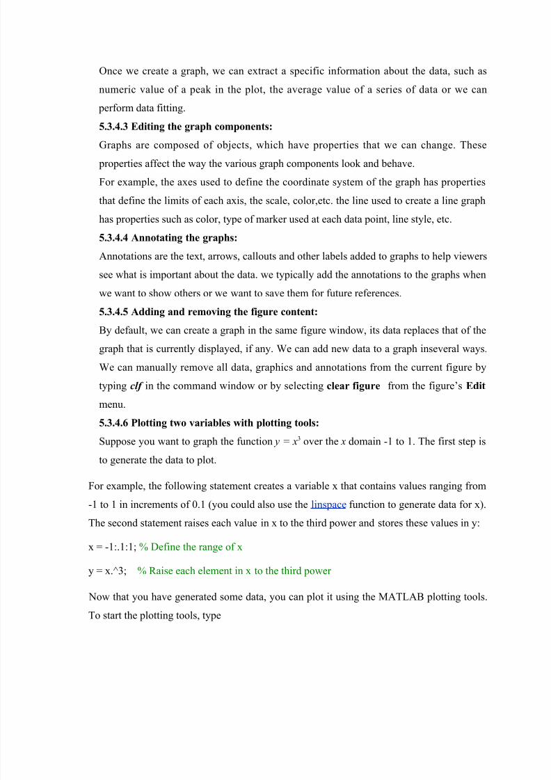
Plottools

A simple line graph is a suitable way to display x as the independent variable and y as the

dependent variable. To do this, select both variables (click to select, and then Shift+click

or Ctrl+click if variables are not contiguous to select again), and then right-click to

display the context menu.



(

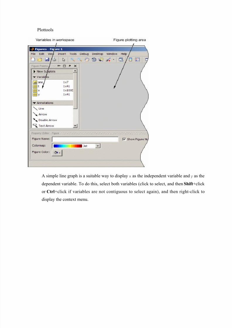
Select plot(x, y) from the menu. The line graph plots in the figure area. The black squares

indicate that the line is selected and you can edit its properties with the Property Editor.

5.3.4.7 Changing the appearance of lines and markers: Change the line properties

so that the graph displays only the data point. Use the Property Editor to set following properties:

Line to no line

Marker to o (circle)

Marker size to 4.0

Marker fill color to red



fig 4

5.3.4.8 Modifying the graph data source: We can link graph data to variables in

your workspace. When you change the values contained in the variables, you can then update

the graph to use the new data without having to create a new graph.

1. Define 50 points between -3π and 3π and compute their sines and cosines:

2. x = linspace(-3*pi,3*pi,50);

3. ys = sin(x);

yc = cos(x);

4. Using the plotting tools, create a graph of ys = sin(x):

5. figure

plottools

6. In the Figure Palette, alternate-click to select x and ys in the Variable pane.

7. Right-click either selected variable and choose plot(x, ys) from the context menu, as the

following figure shows.



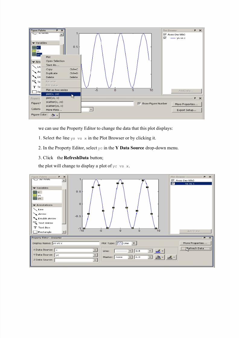
we can use the Property Editor to change the data that this plot displays:

1. Select the line ys vs x in the Plot Browser or by clicking it.

2. In the Property Editor, select yc in the Y Data Source drop-down menu.

3. Click the RefreshData button;

the plot will change to display a plot of yc vs x.



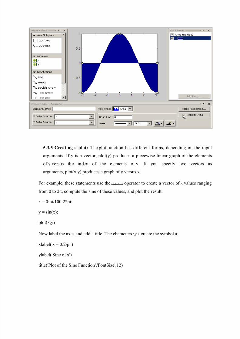
5.3.4.9 Providing new values for the data source:Data values that define the graph are

copies of variables in the base workspace (for example, x and y) to

the XDataand YData properties of the plot object (for example, a lineseries). Therefore, in

addition to being able to choose new data sources, you can assign new values to workspace

variables in the Command Window and click theRefresh Data button to update a graph to

use the new data.

x = linspace(-pi,pi,50); % Define 50 points between -π and π

y = sin(x);

area(x,y) % Make an area plot of x and y

fig7

Now, recalculate y at the command line:

y = cos(x)

Select the blue line on the plot. Select, x as the X Data Source, y as the Y Data Source,

and click Refresh Data. The graph's XData and YData are replaced, making the plot look

like this.



5.3.5 Creating a plot: The plot function has different forms, depending on the input

arguments. If y is a vector, plot(y) produces a piecewise linear graph of the elements

of y versus the index of the elements of y. If you specify two vectors as

arguments, plot(x,y) produces a graph of y versus x.

For example, these statements use the colon operator to create a vector of x values ranging

from 0 to 2π, compute the sine of these values, and plot the result:

x = 0:pi/100:2*pi;

y = sin(x);

plot(x,y)

Now label the axes and add a title. The characters \pi create the symbol π.

xlabel('x = 0:2\pi')

ylabel('Sine of x')

title('Plot of the Sine Function','FontSize',12)

http://www.mathworks.com/access/helpdesk/help/techdoc/ref/plot.html

http://www.mathworks.com/access/helpdesk/help/techdoc/ref/colon.html

http://www.mathworks.com/access/helpdesk/help/techdoc/ref/plot.html

http://www.mathworks.com/access/helpdesk/help/techdoc/ref/colon.html



5.3.5.1 Plotting multiple data sets in one graph :Multiple x-y pair arguments create

multiple graphs with a single call to plot. automatically cycle through a predefined (but

customizable) list of colors to allow discrimination among sets of data. See the

axes ColorOrder and LineStyleOrder properties.

For example, these statements plot three related functions of x, with each curve in a separate

distinguishing color:

x = 0:pi/100:2*pi;

y = sin(x);

y2 = sin(x-.25);

y3 = sin(x-.5);

plot(x,y,x,y2,x,y3)

The legend command provides an easy way to identify the individual plots:

legend('sin(x)','sin(x-.25)','sin(x-.5)')

http://www.mathworks.com/access/helpdesk/help/techdoc/ref/axes_props.html#ColorOrder

http://www.mathworks.com/access/helpdesk/help/techdoc/ref/axes_props.html#LineStyleOrder

http://www.mathworks.com/access/helpdesk/help/techdoc/ref/legend.html

http://www.mathworks.com/access/helpdesk/help/techdoc/ref/axes_props.html#ColorOrder

http://www.mathworks.com/access/helpdesk/help/techdoc/ref/axes_props.html#LineStyleOrder

http://www.mathworks.com/access/helpdesk/help/techdoc/ref/legend.html



5.3.5.2 Specifying the line styles and colors: It is possible to specify color, line styles, and

markers (such as plus signs or circles) when you plot your data using the plot command:

plot(x,y,'color_style_marker ')

color_style_marker is a string containing from one to four characters (enclosed in single

quotation marks) constructed from a color, a line style, and a marker type. The strings are

composed of combinations of the following elements:

Type Values Meanings

Color 'c'

'm'

'y'

'r'

'g'

'b'

'w'

'k'

cyan

magenta

yellow

red

green

blue

white

black

Line style '-'

'--'

':'

'.-'

no character

solid

dashed

dotted

dash-dot

no line



Type Values Meanings

Marker type '+'

'o'

'*'

'x'

's'

'd'

'^'

'v'

'>''<'

'p'

'h'

no character ornone

plus mark

unfilled circle

asterisk

letter x

filled square

filled diamond

filled upward triangle

filled downward triangle

filled right-pointing trianglefilled left-pointing triangle

filled pentagram

filled hexagram

no marker

5.3.5.3 Displaying multiple outputs in one figure: The subplot command enables you to

display multiple plots in the same window or print them on the same piece of paper. Typing

subplot(m,n,p)

partitions the figure window into an m-by-n matrix of small subplots and selects the pth

subplot for the current plot. The plots are numbered along the first row of the figure

window, then the second row, and so on. For example, these statements plot data in four

different subregions of the figure window:

t = 0:pi/10:2*pi;

[X,Y,Z] = cylinder(4*cos(t));

subplot(2,2,1); mesh(X)

subplot(2,2,2); mesh(Y)

subplot(2,2,3); mesh(Z)

http://www.mathworks.com/access/helpdesk/help/techdoc/ref/subplot.html

http://www.mathworks.com/access/helpdesk/help/techdoc/ref/subplot.html



subplot(2,2,4); mesh(X,Y,Z)

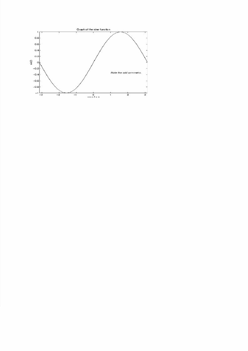
5.3.5.4 Adding labels and titles: The xlabel, ylabel, and zlabel commands add x-, y-,

and z -axis labels. The title command adds a title at the top of the figure and

the text function inserts text anywhere in the figure.

You can produce mathematical symbols using LaTeX notation in the text string, as the

following example illustrates:

t = -pi:pi/100:pi;

y = sin(t);

plot(t,y)

axis([-pi pi -1 1])

xlabel('-\pi \leq {\itt} \leq \pi')

ylabel('sin(t)')

title('Graph of the sine function')

text(1,-1/3,'{\itNote the odd symmetry.}')

http://www.mathworks.com/access/helpdesk/help/techdoc/ref/xlabel.html

http://www.mathworks.com/access/helpdesk/help/techdoc/ref/ylabel.html

http://www.mathworks.com/access/helpdesk/help/techdoc/ref/zlabel.html

http://www.mathworks.com/access/helpdesk/help/techdoc/ref/title.html

http://www.mathworks.com/access/helpdesk/help/techdoc/ref/text.html

http://www.mathworks.com/access/helpdesk/help/techdoc/ref/xlabel.html

http://www.mathworks.com/access/helpdesk/help/techdoc/ref/ylabel.html

http://www.mathworks.com/access/helpdesk/help/techdoc/ref/zlabel.html

http://www.mathworks.com/access/helpdesk/help/techdoc/ref/title.html

http://www.mathworks.com/access/helpdesk/help/techdoc/ref/text.html



Documents

Basic Matlab Material